2007 American WJTA Conference and Expo August 19-21, 2007 Houston, Texas

Paper

NUMERICAL APPROXIMATION OF PROPELLANT DRIVEN

WATER PROJECTILE LAUNCHERS

K. Kluz, E.S. Geskin, O.P. Petrenko New Jersey Institute of Technology

Newark, New Jersey, U.S.A.

ABSTRACT

The objective of this work is to design a reliable, transparent numerical model of the propellant driven water projectile launcher. The fundamentals of interior ballistics, behavior of water as compressible fluid in high-pressure system, and numerical modeling are explained. The CFD approximation, which is a computational copy of the existing experimental system, calculates several values of interest like distribution of velocity, pressure, and volume fraction, and mass flow through the exit boundary. Next, the comparison with empirically obtained values is performed. This work constitutes fundamentals for future optimization research on achieving hypersonic speeds in portable systems, which will allow designing commercial tool for high-speed drilling and military applications.

Organized and Sponsored by the WaterJet Technology Association

1. INTRODUCTION A high-speed liquid projectile (1-2 km/s) could exert pressure in the order of several GPa on an impacted surface and deliver hundreds of megawatts in power. This makes it possible to utilize a liquid impact as a material processing tool. Several devices generating high-speed water projectiles were successfully tested in rock mining industry [1, 7]. Promising experimental results were also achieved in metal forming, stamping, and forging in macro and micro scales [4]. A device accelerating water to high speed and forming water projectile is termed the water launcher. As in a conventional gun, energy needed for water acceleration is provided by fast burning of a propellant, e.g. commercially available smokeless powder. The generated high-pressure combustion products expel water through a tapered, converging nozzle, where the internal energy accumulated in the course of the water compression is used for liquid acceleration. The generated water projectile travels with high velocity and exert extremely high pressure on an impacted target. A bench scale setup (Fig. 1.1) was developed by the Waterjet Technology laboratory in order to investigate the projectiles formation and the projectile-target interaction. Particularly, this setup was used to validate a numerical model of water acceleration in the launcher. Because the measurement of the values like pressure or velocity distribution inside of the barrel is difficult if not impossible, the use of a numerical model is the only approach. A previous process model developed by Atanov [1] and codified by Petrenko et al [8, 9] is applied to a compressible inviscid liquid obeying to the Teta equation. Atanov has applied method of characteristics and Godunov method to solve a system including the mass and momentum balance equations, the state equation (the Teta equation) and the isentropic condition. The system includes only one coordinate and disregard the radial fluid flow. This approach takes no notice of the effects energy dissipation due to liquid viscosity and a boundary layer. It also does not explain the phenomenology of the liquid acceleration in the launcher. The objective of this paper is to develop and validate a process model which does not include assumption above and thus will provide more accurate process description. The presented model seeks to describe unsteady 2D, axisymmetric viscous flow. A commercial CFD software FLUENT® is applied for solving a selected system of equations. This package provides a graphical interface, which enables us to visualize the projectile formation. Also the FLUENT has built in user-defined functions, macros, and surface monitors. These enhancements open a new path to understanding of the physics the projectile generation. 2. EXPERIMENTAL FUNDATION OF CFD MODEL A launcher used for process description is depicted in Figure 2.1. In the course of the experimental study the launcher was loaded with 8 gm of water and the 9 mm blank cartridge filled with 1.18 gm of smokeless powder. The process was initiated by a primer.

The burning of the propellant generated a large amount of gasses initially under high pressure. The generated combustion products drove water toward the nozzle at an increasing velocity. In the converging nozzle water acceleration continued due to internal-to-kinetic energy conversion. The generated projectiles were used for granite boring [4]. In order to investigate projectile motion between the exit of the launcher and a target, the projectile motion was recorder by a high-speed movie camera (see Fig. 2.2). The velocity measured by this camera ranged between 530 m/s and 840 m/s. Also projectile pulsation with period of 344-375 μs was observed. These data were acquired in five consecutive experiments. 3. NUMERICAL MODEL OF PROPELLANT COMBUSTION A numerical model of unsteady propellant combustion describing the boundary conditions at the gas-liquid interface was developed, codified in C++ and incorporated as an user defined function the in Fluent® CFD model. The outcome of the calculation was the average pressure Pa generated by the burning solid propellant in a variable volume system. An analytical procedure suggested by Krier [3] was used for description of the propellant combustion at the following assumption:

• Powder combustion is an adiabatic process • At time t=0 all grains are ignited simultaneously, • The composition of the combustion products is uniform over the occupied space

and constant in the course of time • All exposed grain surface recede at an uniform rate • Noble-Abel equation (see Eq. 3.1) is the state equation of combustion products

FPg

a =⎥⎥⎦

⎤

⎢⎢⎣

⎡−⎟

⎟⎠

⎞⎜⎜⎝

⎛⋅ η

ρ1 (3.1)

At any given time, t the following system of equations describes an adiabatic combustion:

),(),(

)(aT

iapa PtV

QPtzmFtP

+⋅⋅= (3.2)

⎥⎦

⎤⎢⎣

⎡−⋅+⋅−+= )1(),(1),(),(

sa

spaVOFcaT PtzmPtVVPtV

ρη

ρ (3.3)

The integral part of the equations 3.2 and 3.3 is the time dependent parameter z (t,Pa), describing the mass fraction of the propellant burnt.

p

agpa m

PtmmPtz

),(),(

−= (3.4)

At t=0s, z(0)=0 and once the all propellant is burnt z=1. In order to evaluate this parameter the burn rate has to be determined first. A steady state burn rate dx/dt is the speed, at which the least linear grain dimension D recedes. The variable f represents the fraction of D that remaining unburnt. Both f and D are proportional to the pressure that propellant grains are subjected to (Equation 3.5):

)(tPdtdfD

dtdx

a⋅=⋅= β (3.5)

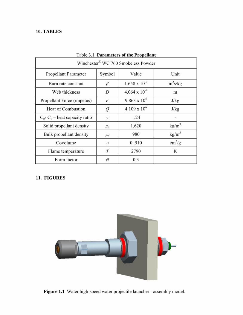
Table 3.1 contains parameters used in numerical and experimental model. The data included in the table for commercially available smokeless powder WC 760. Next, the effect of grain shape on propellant burning must be taken into consideration. There are several geometrical forms of the propellant commercially available like cylindrical, tubular, flake or ball shape. This particular variation is reflected by the constant defined as form factor Ө. The form factor is incorporated in the equation for mass fraction burnt [2]:

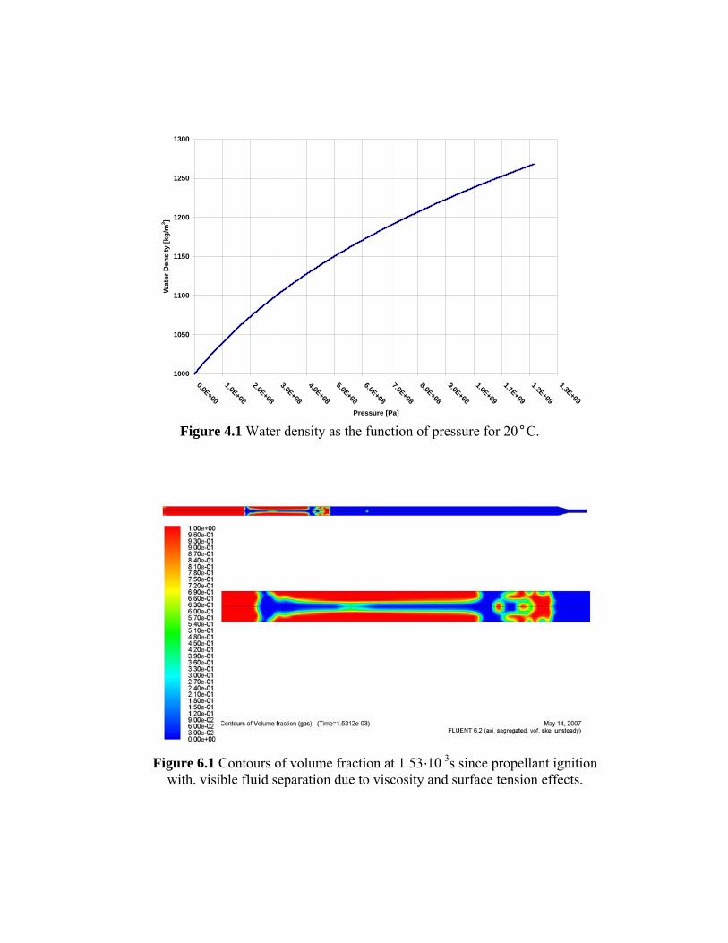
2),( fffPtz a ⋅+⋅−= θθ . (3.6) Another time dependent variable, used in Equation 3.3, is the change of the volume of the combustion products due to the water displacement, VVOF(t,Pa). The value of this variable is provided by Fluent® via the volume fraction cell looping process. Before each iteration, the CDF package enhanced by the user defined C++ function loops of through every cell of the model and evaluates the volumetric fraction of the each phase. The value VVOF(t,Pa) is acquired and used directly in Equation 3.3 . Than the C++ program supported with Fluent® custom macros solves the system of differential equations (3.2-3.6) and determines the pressure Pa on the pressure inlet boundary, which is the final result. 4. WATER AS COMMPRESSIBLE MEDIUM The extremely high pressure developed in the launcher made it necessary to account for the water compressibility. The maximum calculated water pressures in the launcher model were exceeding 1 GPa. Thus, the density of water as the function of pressure ρw(p) as well as the speed of traveling waves as the function of water density ρw and bulk modulus B have to be calculated. Bulk modulus is a property of an elastic medium and is defined as the ratio of the pressure change to the corresponding volume change. Olsen [6] provides an empirical equation for the density of water as the function of pressure (equation is valid for 20°C):

162.0

0 3.65422E81)( ⎟

⎠⎞

⎜⎝⎛ +⋅=

ppw ρρ (4.1)

Graphical representation of the equation 4.1 is depicted in Figure 4.1. The speed of wave propagation or speed of sound in an elastic medium, at a steady temperature is determined by equation

)()(

pBpa

wρ= (4.2)

Equations 4.1 and 4.2 were used in Fluent® CFD modeling as C++ user defined functions. During calculations performed by CFD package these variables were updated before each iteration, based on the data from the previous one. 5. CFD MODEL A segregated, axisymetric, volume of fluid model has been used in the course of the performed computations. The segregated solver is the solution algorithm, which solves sequentially the governing equations. Because the governing equations are non-linear, several iterations of the solution loop must be performed before a model is converged. The diagram of the water launcher segregated model is presented in Figure 5.1. The volume of the fluid model is based on two fluids that do not mix. The volumetric phase composition for each is introduced. In each control volume, a sum up of the volume fractions of all phases is a unity. The process variables and as well as the fluids properties at any given cell are either purely representative of one of the phases, or representative of a mixture of the phases, depending upon the volume fraction of different phases. The process which occurs in the water launcher involves the interaction of two non-penetrable fluids, liquid water and the combustion products. The program limitations prevent modeling of a system containing two compressible fluids. Because the gaseous phase (the combustion products) is assumed to be rigid fluid. This approximation is a reasonable one since the mass of the combustion products is small comparing to the water load, and thus the amount of energy needed to accelerate it is rather small. Moreover, the gas pressure of is governed by the Noble-Abel equation of state (see Equation 3.1) via the C++ macro and therefore the compressibility of the gas is embedded indirectly in the performed numerical analysis. 6. RESULTS The performed computations involved 60,000 time steps. The duration of each step ranged from 1·10-8 –to 1·10-7 s. Each time step involved 10-30 iteration, number of which was determined by the convergence of the computational results. The average computing time for a computer with Intel CentrinoTM 1.6GHz processor is 20 hours, while the actual time of the whole phenomena is approximately 4.5·10-3 s. This statistics demonstrates the complexity of performed calculations. The CFD package used, gives an option to track the values like volume fraction, distribution of pressure and velocity, and density. The values can be retrieved at any time of unsteady state modeling. Figure 6.1 represents sample snapshot of volume fraction distribution at 1.53·10-3s from propellant ignition

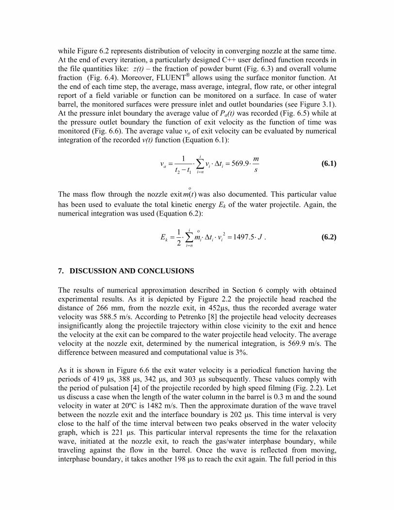
while Figure 6.2 represents distribution of velocity in converging nozzle at the same time. At the end of every iteration, a particularly designed C++ user defined function records in the file quantities like: z(t) – the fraction of powder burnt (Fig. 6.3) and overall volume fraction (Fig. 6.4). Moreover, FLUENT® allows using the surface monitor function. At the end of each time step, the average, mass average, integral, flow rate, or other integral report of a field variable or function can be monitored on a surface. In case of water barrel, the monitored surfaces were pressure inlet and outlet boundaries (see Figure 3.1). At the pressure inlet boundary the average value of Pa(t) was recorded (Fig. 6.5) while at the pressure outlet boundary the function of exit velocity as the function of time was monitored (Fig. 6.6). The average value va of exit velocity can be evaluated by numerical integration of the recorded v(t) function (Equation 6.1):

smtv

ttv

i

niiia ⋅=Δ⋅⋅

−= ∑

=

9.5691

12

(6.1)

The mass flow through the nozzle exitο

)(tm was also documented. This particular value has been used to evaluate the total kinetic energy Ek of the water projectile. Again, the numerical integration was used (Equation 6.2):

JvtmEi

niiiik ⋅=⋅Δ⋅⋅= ∑

=

5.149721 2

ο

. (6.2)

7. DISCUSSION AND CONCLUSIONS The results of numerical approximation described in Section 6 comply with obtained experimental results. As it is depicted by Figure 2.2 the projectile head reached the distance of 266 mm, from the nozzle exit, in 452µs, thus the recorded average water velocity was 588.5 m/s. According to Petrenko [8] the projectile head velocity decreases insignificantly along the projectile trajectory within close vicinity to the exit and hence the velocity at the exit can be compared to the water projectile head velocity. The average velocity at the nozzle exit, determined by the numerical integration, is 569.9 m/s. The difference between measured and computational value is 3%. As it is shown in Figure 6.6 the exit water velocity is a periodical function having the periods of 419 μs, 388 μs, 342 μs, and 303 μs subsequently. These values comply with the period of pulsation [4] of the projectile recorded by high speed filming (Fig. 2.2). Let us discuss a case when the length of the water column in the barrel is 0.3 m and the sound velocity in water at 20ºC is 1482 m/s. Then the approximate duration of the wave travel between the nozzle exit and the interface boundary is 202 μs. This time interval is very close to the half of the time interval between two peaks observed in the water velocity graph, which is 221 μs. This particular interval represents the time for the relaxation wave, initiated at the nozzle exit, to reach the gas/water interphase boundary, while traveling against the flow in the barrel. Once the wave is reflected from moving, interphase boundary, it takes another 198 μs to reach the exit again. The full period in this

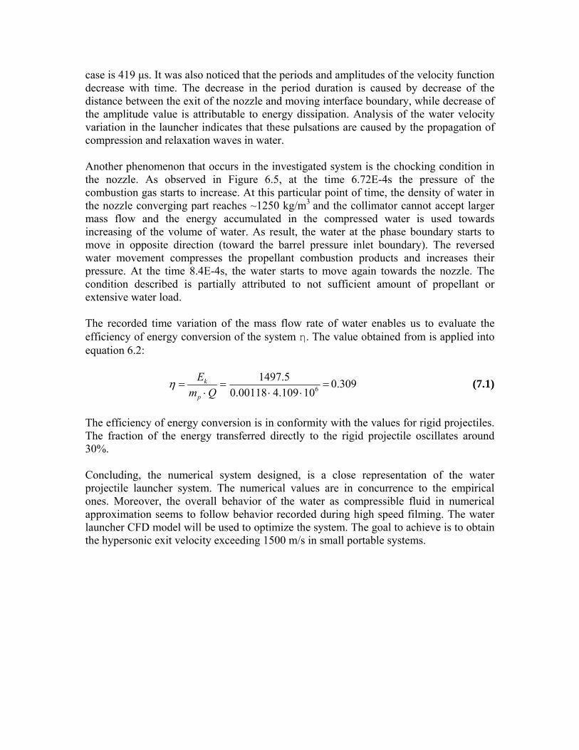
case is 419 μs. It was also noticed that the periods and amplitudes of the velocity function decrease with time. The decrease in the period duration is caused by decrease of the distance between the exit of the nozzle and moving interface boundary, while decrease of the amplitude value is attributable to energy dissipation. Analysis of the water velocity variation in the launcher indicates that these pulsations are caused by the propagation of compression and relaxation waves in water. Another phenomenon that occurs in the investigated system is the chocking condition in the nozzle. As observed in Figure 6.5, at the time 6.72E-4s the pressure of the combustion gas starts to increase. At this particular point of time, the density of water in the nozzle converging part reaches ~1250 kg/m3 and the collimator cannot accept larger mass flow and the energy accumulated in the compressed water is used towards increasing of the volume of water. As result, the water at the phase boundary starts to move in opposite direction (toward the barrel pressure inlet boundary). The reversed water movement compresses the propellant combustion products and increases their pressure. At the time 8.4E-4s, the water starts to move again towards the nozzle. The condition described is partially attributed to not sufficient amount of propellant or extensive water load. The recorded time variation of the mass flow rate of water enables us to evaluate the efficiency of energy conversion of the system η. The value obtained from is applied into equation 6.2:

=⋅⋅

=⋅

= 610109.400118.05.1497

QmE

p

kη 0.309 (7.1)

The efficiency of energy conversion is in conformity with the values for rigid projectiles. The fraction of the energy transferred directly to the rigid projectile oscillates around 30%. Concluding, the numerical system designed, is a close representation of the water projectile launcher system. The numerical values are in concurrence to the empirical ones. Moreover, the overall behavior of the water as compressible fluid in numerical approximation seems to follow behavior recorded during high speed filming. The water launcher CFD model will be used to optimize the system. The goal to achieve is to obtain the hypersonic exit velocity exceeding 1500 m/s in small portable systems.

8. REFERENCES 1. Atanov G. A. Hydro-Impulsive Installations for Rocks Breaking, Vishaia Shkola, Kiev, Ukraine, 1987 2. Corner, J., Theory of the Internal Ballistics of Guns, John Wiley and Sons, New York and London, 1950 3. Krier H., Adams M., An Introduction to Gun Interior Ballistics and a Simplified Ballistic Code, Progress in Astronautics and Aeronautics, American Institute of Aeronautics and Astronautics, invited paper, June 1978 4. Samardzic V., Micro, Meso and Macro Materials Processing Using High Speed Water Projectiles, Ph.D Dissertation, Department of Mechanical Engineering, NJIT, May 2007 5. Cappock Advanced Interior Ballistic Model, the freeware software developed by Fabrique Scientific® in 1995 6. Olsen J. H., Abrasive Jet Mechanics, published at www.thefabricator.com, March, 2005 7. Petrenko O., Investigation of Material Fracturing by High Speed Water Slug, 16th Itnl. Symposium on Jet Cutting Technology, BHRA, Cranfielid, England, 2002 8. Petrenko O., Geskin E.S., Atanov G., Semko A., Goldenberg B., Numerical Modeling of Formation of High-Speed Water Slugs, ASME Transaction, Journal of Fluids Engineering, March 2004, pp. 206-209 9. Petrenko O., Investigation of Formation and Development of High-Speed Liquid Projectiles, Ph.D Thesis, NJIT, 2007

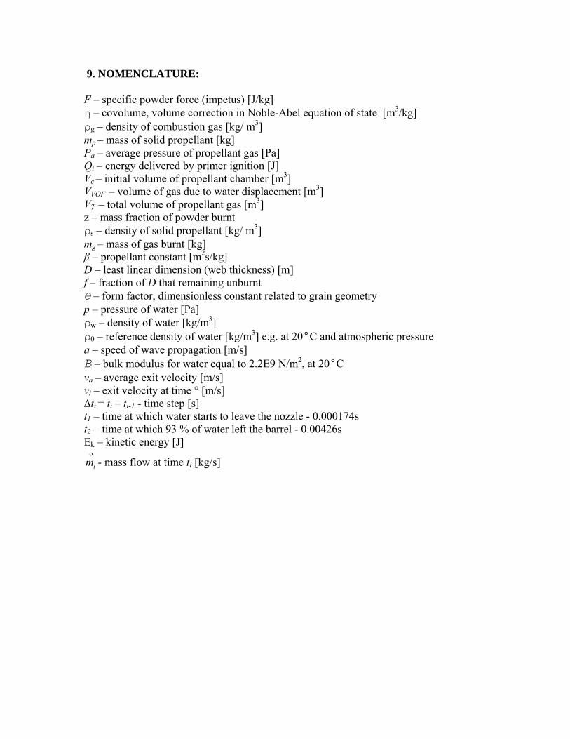
9. NOMENCLATURE: F – specific powder force (impetus) [J/kg] η – covolume, volume correction in Noble-Abel equation of state [m3/kg] ρg – density of combustion gas [kg/ m3] mp – mass of solid propellant [kg] Pa – average pressure of propellant gas [Pa] Qi – energy delivered by primer ignition [J] Vc – initial volume of propellant chamber [m3] VVOF – volume of gas due to water displacement [m3] VT – total volume of propellant gas [m3] z – mass fraction of powder burnt ρs – density of solid propellant [kg/ m3] mg – mass of gas burnt [kg] β – propellant constant [m2s/kg] D – least linear dimension (web thickness) [m] f – fraction of D that remaining unburnt Ө – form factor, dimensionless constant related to grain geometry p – pressure of water [Pa] ρw – density of water [kg/m3] ρ0 – reference density of water [kg/m3] e.g. at 20°C and atmospheric pressure a – speed of wave propagation [m/s] B – bulk modulus for water equal to 2.2E9 N/m2, at 20°C va – average exit velocity [m/s] vi – exit velocity at time ° [m/s] ∆ti = ti – ti-1 - time step [s] t1 – time at which water starts to leave the nozzle - 0.000174s t2 – time at which 93 % of water left the barrel - 0.00426s Ek – kinetic energy [J]

ο

im - mass flow at time ti [kg/s]

10. TABLES

Table 3.1 Parameters of the Propellant

Winchester® WC 760 Smokeless Powder

Propellant Parameter Symbol Value Unit

Burn rate constant β 1.658 x 10-9 m2s/kg

Web thickness D 4.064 x 10-4 m

Propellant Force (impetus) F 9.863 x 105 J/kg

Heat of Combustion Q 4.109 x 106 J/kg

Cp/ Cv – heat capacity ratio γ 1.24 -

Solid propellant density ρs 1,620 kg/m3

Bulk propellant density ρs 980 kg/m3

Covolume η 0 .910 cm3/g

Flame temperature T 2790 K

Form factor Ө 0.3 - 11. FIGURES

Figure 1.1 Water high-speed water projectile launcher - assembly model.

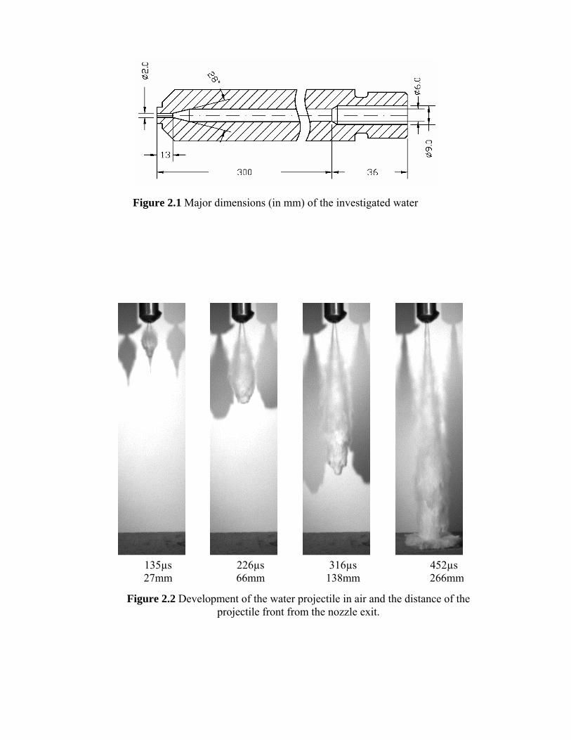
Figure 2.1 Major dimensions (in mm) of the investigated water

135µs 226µs 316µs 452µs 27mm 66mm 138mm 266mm

Figure 2.2 Development of the water projectile in air and the distance of the projectile front from the nozzle exit.

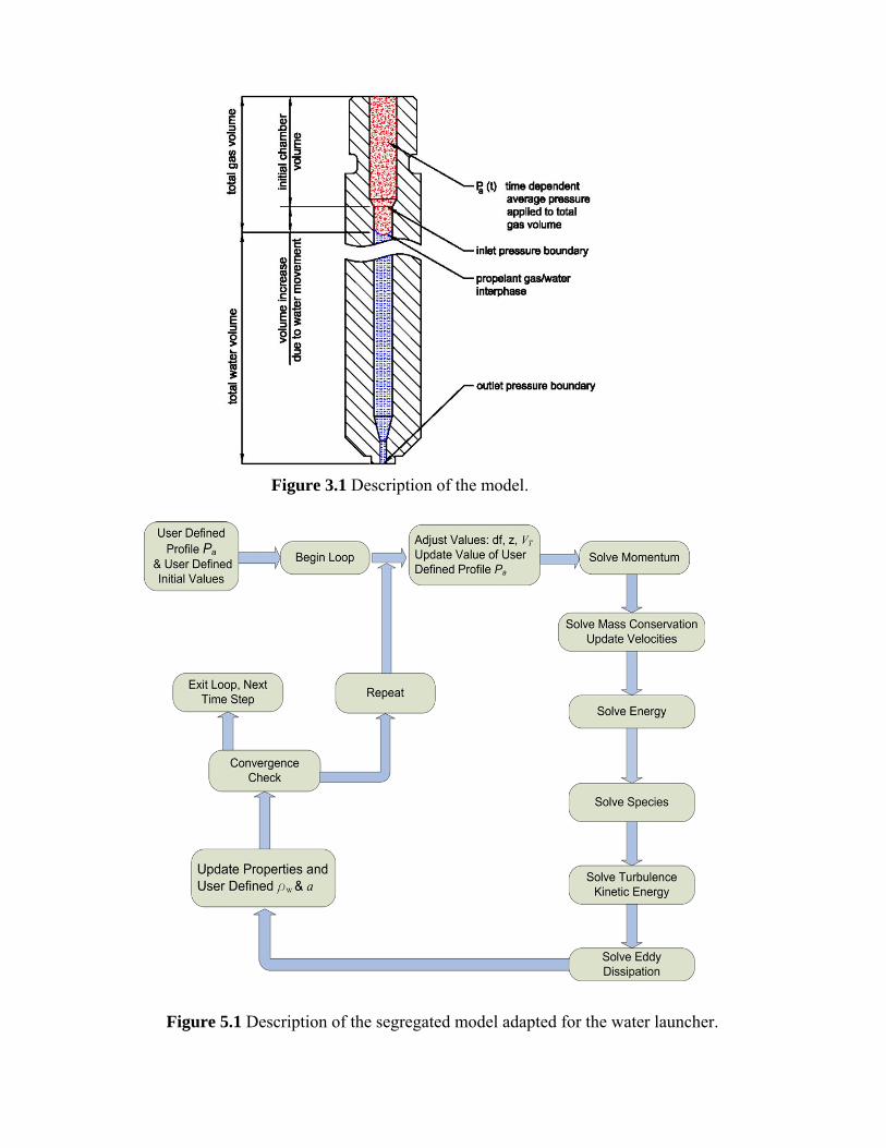
Figure 3.1 Description of the model.

Figure 5.1 Description of the segregated model adapted for the water launcher.

1000

1050

1100

1150

1200

1250

1300

0.0E+00

1.0E+08

2.0E+08

3.0E+08

4.0E+08

5.0E+08

6.0E+08

7.0E+08

8.0E+08

9.0E+08

1.0E+09

1.1E+09

1.2E+09

1.3E+09

Pressure [Pa]

Wat

er D

ensi

ty [k

g/m

3 ]

Figure 4.1 Water density as the function of pressure for 20°C.

Figure 6.1 Contours of volume fraction at 1.53·10-3s since propellant ignition with. visible fluid separation due to viscosity and surface tension effects.

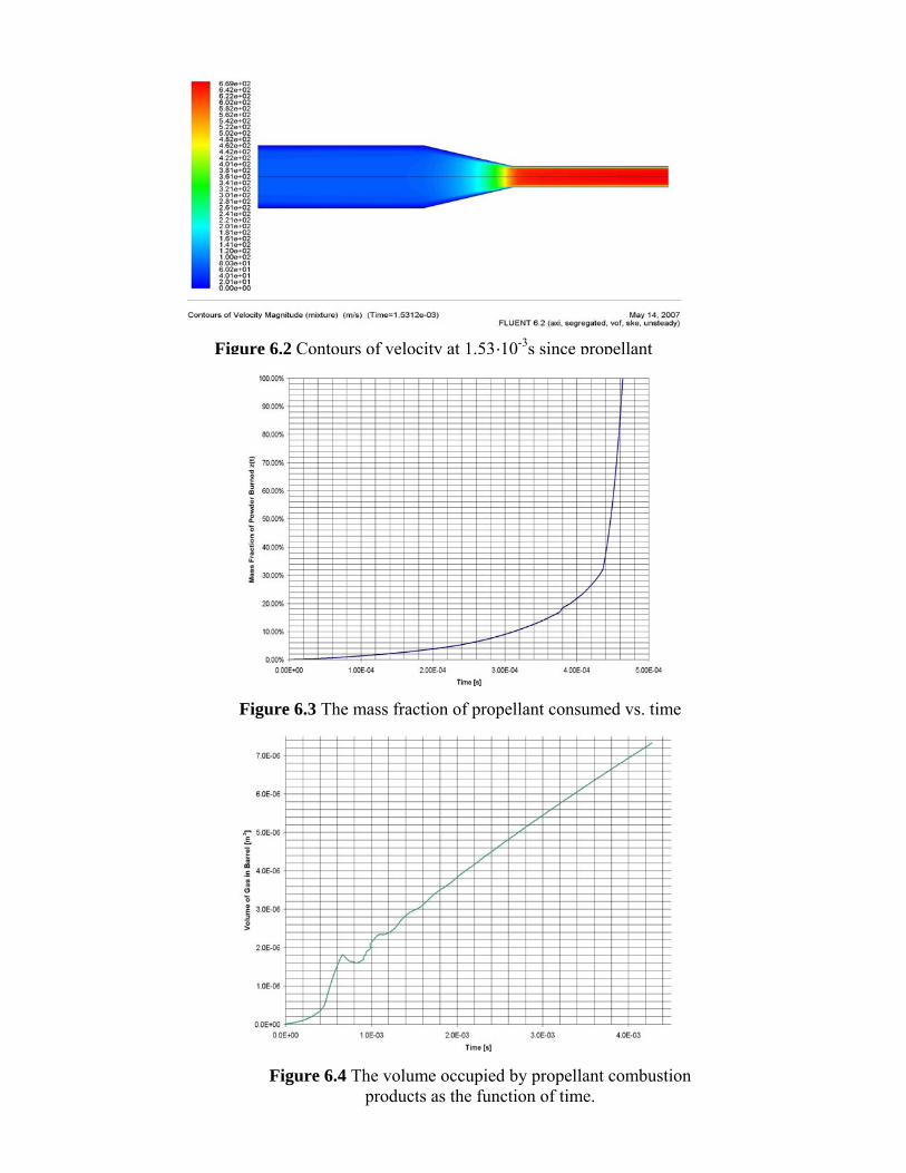
Figure 6.2 Contours of velocity at 1.53·10-3s since propellant

Figure 6.3 The mass fraction of propellant consumed vs. time

Figure 6.4 The volume occupied by propellant combustion products as the function of time.

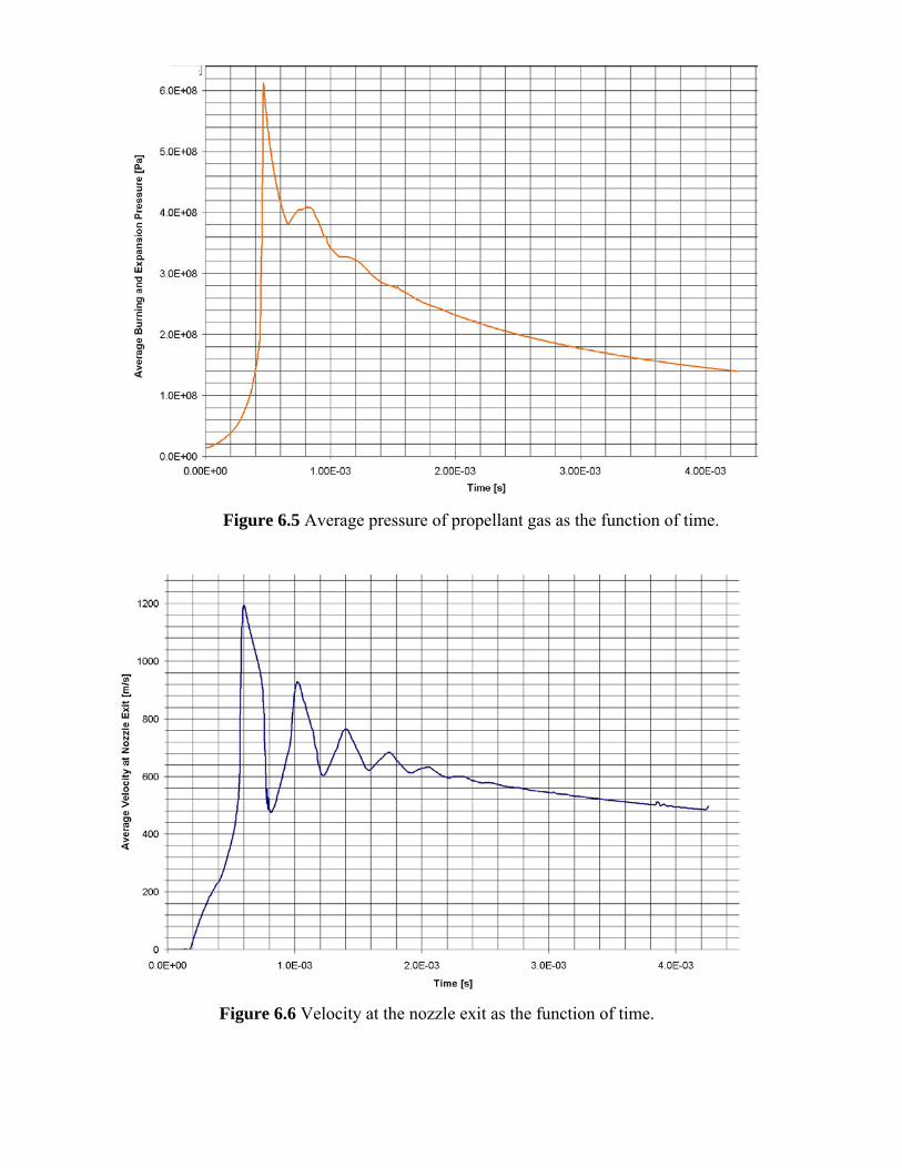
Figure 6.5 Average pressure of propellant gas as the function of time.

Figure 6.6 Velocity at the nozzle exit as the function of time.