numerical approach to differential equations of … · methods for ordinary differential equations....
TRANSCRIPT

Global Journal of Pure and Applied Mathematics.
ISSN 0973-1768 Volume 13, Number 9 (2017), pp. 5813-5826
© Research India Publications
http://www.ripublication.com
Numerical Approach to Differential Equations of
Fractional order Bratu-type Equations by
Differential Transform Method
Mukesh Grover* and Dr. Arun Kumar Tomer**
*Department of Mathematics, GZS Campus College of Engineering & Technology
Maharaja Ranjit Singh Punjab Technical University, Bathinda, Punjab, India.
**Department of Mathematics S.M.D.R.S.D College Pathankot, Punjab, India.
Abstract
In the present paper, the Differential Transform Method (DTM) is applied to
drive its solution (approximate) of the fractional Bratu-type equations. The
fractional derivatives are represented in the caputo sense. The convergence
and uniqueness of this method are also studied. Three examples are illustrated
to prove that the presented techniques efficiency and implementation of the
method and the results are compared with exact solutions.
Keywords: Fractional Bratu-type equations, Caputo fractional derivatives,
Differential Transform Method, Numerical Solutions.
1. INTRODUCTION:
We know that Fractional calculus is playing vital role in the field of Mathematics. It
deals with derivatives and integral of arbitrary orders. Fractional differential equations
and its results used in general in many branches of mathematics and deals with
Science and Engineering also. Many effective different techniques for solving its
numerical and analytical solutions of FDEs have been presented [6-8].
We have used notations nD for Jumarie type fractional derivative operator here
1, n . There are many types of fractional integral and differential operators.
5814 Mukesh Grover and Dr. Arun Kumar Tomer
Since proposed in (Zhou, 1986), there is good interest on the applications of
Differential Transform Method (DTM) to solve various scientific problems. The
DTM [1-2,10-12,14-15] is an approximation to the exact solution of the functions
which are differentiable in the form of polynomials. The DTM is an alternative
procedure for getting Taylor series solution of the differential equations. This method
reduces the size of computational domain and is easily applicable to many problems.
Large list of methods, exact, approximate and purely numerical are available for the
solution of differential equations. Most of these methods are computationally
intensive because they are a trial-and error in nature, or need complicated symbolic
computations. The differential transformation technique is one of the numerical
methods for ordinary differential equations. This method constructs a semi-analytical
numerical technique that uses Taylor series for the solution of differential equations in
the form of a polynomial. It is different from the high-order Taylor series method
which requires symbolic computation of the necessary derivatives of the data
functions. For the calculation of Bratu-type equation with the help of differential
transform method with constant value of
)1.1(,0)0(,0)0(,10,10,0exp2
uuxuuDt
These days, a massive quantity of kinds of literature advanced concerning with FDEs
in nonlinear dynamics [3-5]. On the grounds that maximum fractional differential
equations do now not have genuine analytic answers, approximation, and numerical
techniques, consequently, they are used substantially. lately, the Adomian
decomposition technique, Homotopy analysis method and new iterative method were
used for decision a large range of problems [9,13,16].
2. CAPUTO FRACTIONAL DERIVATIVE:
On this paper, there are many definitions of a fractional derivative of order α > 0. The
two most normally used definitions like as the Riemann–Liouville and Caputo. Each
definition makes use of Riemann–Liouville fractional integration and derivatives of
the whole order.
Let )(,: xfxRRf , denote a continuous function, and let the partition 0h in
the interval ].1,0[ Through the fractional Riemann Liouville integral
)1.2(,0,)(
1)(
0
1
0
x
x
x dttftxxfI
the modified Riemann-Liouville derivative is defined as
Numerical Approach to Differential Equations of Fractional order Bratu-type.. 5815
)2.2(,))0()((
1)(
0
0
xn
n
n
x dtftftxdx
d
nxfD
]1,0[, xwhere
.1,1 nnn
The difference between the two definitions is in the order of evaluation. Riemann–
Liouville fractional integration of order α is outlined as
3.2,0,0,)(
1)(
0
0
1
xdttftxxfJ
x
x
x
)()(0
xfJdx
dxfD m
m
m
x
)4.2(,)()(0
*
xf
dx
dJxfD
m
mm
x
where mm 1 and m ∈ N. For now, the Caputo fractional by-product can be
denoted by using
*D to maintain a clear difference with the Riemann–Liouville
fractional derivative. The Caputo fractional derivative is also defined as follows
)5.2(),1(,
)(
)(1)(
0
1Nnnnd
t
f
ntfD
t
t
n
n
t
Suppose that in DTM of kth derivative of function f(t).
)6.2()()1(
1)(
00 tt
k
x tfDk
kF
and the inverse of DTM as follows:
)7.2())(()( 0
0
k
i
ttkFtf
The following properties of DTM, Let f(t), u(t), v(t) change into )(),(),( kVkUkF
)()()()(
)()()()()()(
kUkFtutf
kVkUkFtvtutf
)()()()().()(0
nkUnVkFtvtutfk
n
5816 Mukesh Grover and Dr. Arun Kumar Tomer
2!)()()(
!)()exp()(
)1..().1(!
1)()1()(
)()()......2)(1()()(
)(
kSin
k
akFatSintf
k
akFattf
kmmmk
kFttf
mkUmkkkkFdt
tudtf
k
k
m
m
m
3. MITTAG-LEFFLER FUNCTION:
Mittag-Leffler Function helps to find out the solution of distinct equations like as
fractional order differential, integral equations. The Mittag-Leffler function was
introduced by Gosta Mittag-Leffler in 1903.
From the Jumarie definition of fractional derivative we have 0CDx
Ja
.with the
help of order ( 10 ) of Jumarie derivative with the initial point nxxf )(
Rnxn
nxD nn
x
J
)1(
0 )(1)1(
1)(
)()()(0a
a
a
ax
Ja
ax
J axaEaxEDaxED
(3.1)
)sinh()(cosh)(),sin()(cos)(
xixxExixixE
0
2
0
2
21)(cosh,
21)1()(cos
m
m
m
mm
m
xx
m
xx
0
)12(
0
)12(
)12(1)(sinh,
)12(1)1()(sin
m
m
m
mm
m
xx
m
xx
(3.2)
4. BRATU EQUATION:
Now we have to discuss that Uniqueness and convergence of Bratu equation as
follows:
4.1 Uniqueness of Bratu equation:
If Bratu-type equation has a result, then it is unique whenever, .10 here,
t
L
1and L is a Lipschitz constant.
Numerical Approach to Differential Equations of Fractional order Bratu-type.. 5817
Proof: Bratu-type equation can be written as in the form
t
dxxuxFtu0
)(,1
)(
where
( )
0
1( , ( )) (4.1)
1
t
u xF t u t e dx
such that the nonlinear term ))(,( tutF is Lipschitz continuous with
.),(),( wuLwtFutF
The Lipschitz constant L can be calculated as follows. Using this maximum norm,
10max
tF ))(,( tutF ,
0 !n
nn
wu
n
wuee
1 2 1
1
1... , (4.2)
!
n n n
n
u w u u w wn
Since the series is convergent.
,.............. 1221 nnnn wuwwuu
is bounded n and
1 2 2 1.............. , 1,2,... (4.3)n n n nu u w uw w N n
Therefore
.)1(!
1
0
wueNn
Nwueen
wu
Hence,
t
t
wu
dxwueN
dxeewtFutF
0
0
,1
)1(
1
1),(),(
0
( 1)( , ) ( , )
1
( 1)
1
( 1). (4.4)
1
tN e
F t u F t w u w dx
N e tu w
N eu w
5818 Mukesh Grover and Dr. Arun Kumar Tomer
Then , we can choose L which is
1
)1(eNL
Now, Let u and v be two different solutions of Bratu-type equation, then
t t
dxxvxFdxxuxFvu0 0
)(,1
)(,1
.
1
)()()(1
0
tvuL
dxvFuF
t
,0
11
t
Lvu
vu ,01
t
L
1vu =0,
)5.4(.vu
One important outcome (*) will be there if 0),(exp))(( 0 ttutuf and F(k) is
coefficient of power series in Fractional form ))(( xuf , then
.1
0)0(exp
)()()1)1((
)1(
)1(
)1)1((
)( 1
kwhen
kwhenu
ikFiui
i
k
k
kF
k
i
Where .,........3,2,1,0),()1(
1)( kitattuD
iiU
i
x
For the calculation of Bratu-type equation with the help of differential transform
method
uuDuF t exp)(2
0
)()(u
utuFty
We get, ,)12(
)()(,0)(
2
10
ttutu
0
10 ).(..............)()()(k
k tutututu
Numerical Approach to Differential Equations of Fractional order Bratu-type.. 5819
4.2 Convergence of Bratu equation:
If the series
0
)(k
k tu is convergent to s(t), then it must be the exact solution of
equation (1.1).
Proof: By using above result (*), equation (1.1) can be written as
00
,1,)2()(
2
kwhen
kwhentkUtu
k
k
00
,1)),1(2()12(
)1)1(2(
)2(
k
kkFk
k
kU
Using above result(*),
11
.2
))1(2()2()1)12((
)12(
)1)1(2(
)1)32((
))1(2(
1
1
kwhen
kwhen
ikFiui
i
k
k
kF
k
i
.)2(&)2()(1
2)(
1
2
i
kts
i
k tkFetkUtS Now, S(t) satisfied the bratu-type
equation, therefore we get,
)(exp)(2
tstsDt
.)2()2(1
2
1
22
i
k
i
k
t tkFtkUD
.0)2()1)1(2(
)12()2(
1
2)1(2
1
i
kk
i
tkFtk
kkU
5. ILLUSTRATIVE EXAMPLES
In this section, Differential transform method is applied on Bratu equations. Then, we
get its approximate solutions and exact solutions with different values of . we solve
three examples by DTM as follows:
Example1. Suppose the following type of Fractional Bratu-type Equation
)1.5(,0)(exp2)(2
tutuDt
5820 Mukesh Grover and Dr. Arun Kumar Tomer
with initial conditions )2.5(0)0()0(,10,10 uut
Solution: The exact solution of equation (5.1) when value of α =1 is
)ln(cos2)( ttu
Apply DTM with 00 t and 1 , to both sides of BTE and making use of
properties of DTM. Let ( ) 2exp ( ) 0, (5.3)tD u t u t
0!)1(
)1(
kKY
k
k
)1(
)1(
!2
k
k
kKY (5.4)
Put the values of ,1 ,2 in (5.4), and get the result by putting the values of k =
0, 1, 2, 3, 4, 5, 6…..,n as follows:
,.......45
1)10(,
36
1)9(,
28
1)8(
,21
1)7(,
15
1)6(,
10
1)5(,
6
1)4(
,3
1)3(,1)2(,0)1(,0)0(
111
1111
1111
YYY
YYYY
YYYY
Then takes inverse transformation, we get results with different values of . Now,
four different cases are here, as follows:
0
)()( ttYty
Case I: Evaluate y(t) ,when value of is 0.25.
......)6646.07044.07522.08111.08862.09862.01284.1(2)( 24
7
4
6
4
5
4
3
2
1
ttttttttu
Case II: Evaluate y(t) ,when value of is 0.5.
.........)2222.025.02857.03333.03999.05.06668.0.1(2)( 2
9
42
7
32
5
22
3
tttttttttu
Case III: Evaluate y(t) ,when value of is 0.75.
......)60726.00897.01146.01536.08862.093605.07522.0(2)( 64
21
2
9
4
15
34
9
2
3
ttttttttu
Case IV: Evaluate y(t) ,when value of is 1.

Numerical Approach to Differential Equations of Fractional order Bratu-type.. 5821
......)0277.00357.00476.00666.01.01666.03333.0()( 98765432 tttttttttu
Figure 1.1
This is the approximate solutions of Differential Transformation Method with various
values of alphas like 0.25, 0.50, 0.75 and 1.0. in figure (1.1) and included Exact
solution at alpha is unity.
Example 2. Suppose the following type of Fractional Bratu-type Equation
)5.5(,0)(exp)( 22 tutuDt
with initial conditions )6.5()0()0(,10,10 uut
Solution: The exact solution of equation (5.5) when value of α =1 is
)).sin(1ln()( ttu
Apply DTM with 00 t and 1 , to both sides of Bratu-type Equation and making
use of properties of DTM.
Let )7.5(,0)(exp)( 2 tutuDt
0!)1(
)1(
kKY
k
k
)1(
)1(
!2
k
k
kKY (5.8)
0
5
10
15
20
25
30
35
1 2 3 4 5 6 7 8 9 10 11
Exact Solution α = 1
Approximate Solution α = 1Approximate Solution α = 0.75Approximation Solution α = 0.50
5822 Mukesh Grover and Dr. Arun Kumar Tomer
Put the values of ,1 ,2 in (5.8), and get the result by putting the values of k =
0, 1, 2, ....n similar as in example 1.Then takes inverse transformation; we get results
with different values of . Now, four different cases are here, as follows:
0
)()( ttYty
Case I: Evaluate y(t) ,when value of is 0.25.
......)6646.07044.07522.08111.08862.09862.01284.1(86.9)( 24
7
4
6
4
5
4
3
2
1
ttttttttu
Case II: Evaluate y(t) ,when value of is 0.5.
.........)2222.025.02857.03333.03999.05.06668.0.1(86.9)( 2
9
42
7
32
5
22
3
tttttttttu
Case III: Evaluate y(t) ,when value of is 0.75.
......)60726.00897.01146.01536.08862.093605.07522.0(86.9)( 64
21
2
9
4
15
34
9
2
3
ttttttttu
Case IV: Evaluate y(t) ,when value of is 1.
......)0277.00357.00476.00666.01.01666.03333.0(93.4)( 98765432 tttttttttu
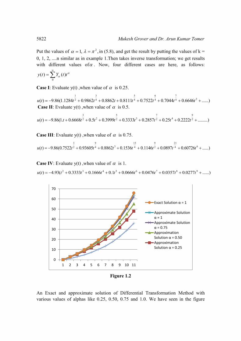
Figure 1.2
An Exact and approximate solution of Differential Transformation Method with
various values of alphas like 0.25, 0.50, 0.75 and 1.0. We have seen in the figure
0
10
20
30
40
50
60
70
1 2 3 4 5 6 7 8 9 10 11
Exact Solution α = 1
Approximate Solution α = 1
Approximate Solution α = 0.75
Approximation Solution α = 0.50
Approximation Solution α = 0.25
Numerical Approach to Differential Equations of Fractional order Bratu-type.. 5823
(1.2.) to reduce the value of alpha that is close to the exact solution with minimum
error.
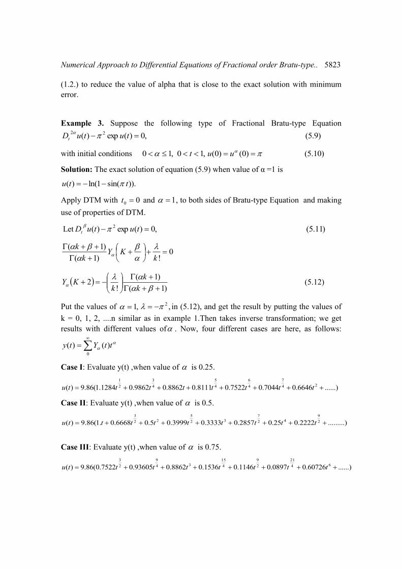
Example 3. Suppose the following type of Fractional Bratu-type Equation
)9.5(,0)(exp)( 22 tutuDt
with initial conditions )10.5()0()0(,10,10 uut
Solution: The exact solution of equation (5.9) when value of α =1 is
)).sin(1ln()( ttu
Apply DTM with 00 t and 1 , to both sides of Bratu-type Equation and making
use of properties of DTM.
Let )11.5(,0)(exp)( 2 tutuDt
0!)1(
)1(
kKY
k
k
)1(
)1(
!2
k
k
kKY (5.12)
Put the values of ,1 ,2 in (5.12), and get the result by putting the values of
k = 0, 1, 2, ....n similar as in example 1.Then takes inverse transformation; we get
results with different values of . Now, four different cases are here, as follows:
0
)()( ttYty
Case I: Evaluate y(t) ,when value of is 0.25.
......)6646.07044.07522.08111.08862.09862.01284.1(86.9)( 24
7
4
6
4
5
4
3
2
1
ttttttttu
Case II: Evaluate y(t) ,when value of is 0.5.
.........)2222.025.02857.03333.03999.05.06668.0.1(86.9)( 2
9
42
7
32
5
22
3
tttttttttu
Case III: Evaluate y(t) ,when value of is 0.75.
......)60726.00897.01146.01536.08862.093605.07522.0(86.9)( 64
21
2
9
4
15
34
9
2
3
ttttttttu
5824 Mukesh Grover and Dr. Arun Kumar Tomer
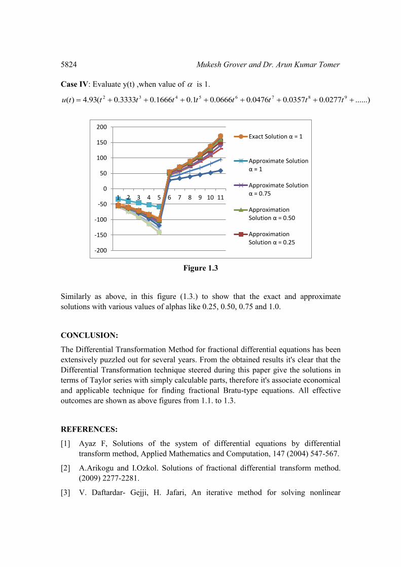
Case IV: Evaluate y(t) ,when value of is 1.
......)0277.00357.00476.00666.01.01666.03333.0(93.4)( 98765432 tttttttttu
Figure 1.3
Similarly as above, in this figure (1.3.) to show that the exact and approximate
solutions with various values of alphas like 0.25, 0.50, 0.75 and 1.0.
CONCLUSION:
The Differential Transformation Method for fractional differential equations has been
extensively puzzled out for several years. From the obtained results it's clear that the
Differential Transformation technique steered during this paper give the solutions in
terms of Taylor series with simply calculable parts, therefore it's associate economical
and applicable technique for finding fractional Bratu-type equations. All effective
outcomes are shown as above figures from 1.1. to 1.3.
REFERENCES:
[1] Ayaz F, Solutions of the system of differential equations by differential
transform method, Applied Mathematics and Computation, 147 (2004) 547-567.
[2] A.Arikogu and I.Ozkol. Solutions of fractional differential transform method.
(2009) 2277-2281.
[3] V. Daftardar- Gejji, H. Jafari, An iterative method for solving nonlinear
-200
-150
-100
-50
0
50
100
150
200
1 2 3 4 5 6 7 8 9 10 11
Exact Solution α = 1
Approximate Solution α = 1
Approximate Solution α = 0.75
Approximation Solution α = 0.50
Approximation Solution α = 0.25
Numerical Approach to Differential Equations of Fractional order Bratu-type.. 5825
functional equations, J. Math. Anal. Appl. 316 (2) (2006) 753–763.
[4] H. Jafari, V. Daftardar-Gejji, Solving a system of nonlinear fractional
differential equations using Adomian decomposition, J. Comput. Appl. Math.
196 (2) (2006) 644–651.
[5] N. Shawagfeh, Analytical approximate solutions for nonlinear fractional
differential equations, Appl. Math. Comput. 131 (2) (2002) 517–529.
[6] S. Momani, Z. Odibat, Numerical approach to differential equations of
fractional order, J. Comput. Appl. Math. (2006), doi:
10.1016/j.cam.2006.07.015.
[7] S. Momani, Z. Odibat, Numerical comparison of methods for solving linear
differential equations of fractional order, Chaos Sol. Fract. 31 (5) (2007) 1248–
1255.
[8] U. Ghosh., S. Sengupta, S. Sarkar and S. Das. Analytic sol. on of linear fract.
diff. Eq. with Jumarie derivative in term of Mittag-Leffler function. AJMA
3(2). 2015. 32-38, 2015. [9] A. A. M. Arafa, S. Z. Rida, H. Mohamed,
Homotopy Analysis Method for Solving Biological Population Model,
Communications in Theoretical Physics, vol.56, No.5, 2011. [10] G. Adomian,
Solving frontier problems of physics: The decomposition method, Kluwer
Academic Publishers, Boston and London, 1994.
[11] Chen C.K., S. S. Chen, Application of the differential transform method to a
non-linear conservative system, Applied Mathematics and Computation
154,(2004) 431-441 5
[12] Kuo B.L. Applications of the differential transform method to the solutions of
the free Problem, Applied Mathematics and Computation 165 (2005) 63-79
[13] HassanI.H. Abdel-Halim Comparison differential transformation technique with
Adomain decomposition method for linear and nonlinear initial value problems,
Choas Solutions Fractals, 36(1): 53-(2008)65.
[14] Erturk, V.S., Momani, S. and Odibat, Z.(2008). application of generalized
differential transform method to multi-order fractional differential equations.
Communications in Nonlinear Science and Numerical Simulation, 13(8), 1642-
1654.
[15] Garg, M. and Manohar, P.(2015). Three-dimensional generalized differential
transform method for space-time fractional diffusion equation, Palestine Journal
of Mathematics, 4(1),127-135.
[16] Grover. Mukesh, Tomer, Arun kumar, A New Technique to Inculcate the
Particular Solution of Fractional Order α { D or 2D or 3D } Differential
Equations With Boundary Conditions, International Journal of Comp. &
5826 Mukesh Grover and Dr. Arun Kumar Tomer
Mathematical Sciences, Volume 6,Issue-5, 2017 p.p.67-75.
[17] V. Daftardar-Gejji, S. Bhalekar, Solving fractional boundary value problems
with Dirichlet boundary conditions using a new iterative method, Computers
& Mathematics with Applications, vol.59, No.5, 2010, pp. 1801-1809.
[18] Grover. Mukesh, Tomer, Arun kumar, Estimate the Solution of Fractional
Differential Equations with Transcendental Functions, Iinternational Journal of
Advanced Research in Computer Science and Software Engineering, Volume 7,
Issue-5, 2017 p.p.971-976.