numerical and experimental studies of …constellation.uqac.ca/424/1/25017555.pdf · comportement...
TRANSCRIPT

UNIVERSITÉ DU QUÉBEC
MEMOIRE PRESENTE AL'UNIVERSITÉ DU QUÉBEC À CHICOUTIMI
COMME EXIGENCE PARTIELLEDE LA MAÎTRISE EN INGÉNIERIE
PAR
MEHRAN MATBOU RIAHI
NUMERICAL AND EXPERIMENTAL STUDIES OF THEMECHANICAL BEHAVIOUR AT THE ICE / ALUMINIUM
INTERFACE
ETUDES NUMERIQUE ET EXPERIMENTALE DUCOMPORTEMENT MÉCANIQUE À L'INTERFACE GLACE /
ALUMINIUM
FEVRIER 2007

Mise en garde/Advice
Afin de rendre accessible au plus grand nombre le résultat des travaux de recherche menés par ses étudiants gradués et dans l'esprit des règles qui régissent le dépôt et la diffusion des mémoires et thèses produits dans cette Institution, l'Université du Québec à Chicoutimi (UQAC) est fière de rendre accessible une version complète et gratuite de cette œuvre.
Motivated by a desire to make the results of its graduate students' research accessible to all, and in accordance with the rules governing the acceptation and diffusion of dissertations and theses in this Institution, the Université du Québec à Chicoutimi (UQAC) is proud to make a complete version of this work available at no cost to the reader.
L'auteur conserve néanmoins la propriété du droit d'auteur qui protège ce mémoire ou cette thèse. Ni le mémoire ou la thèse ni des extraits substantiels de ceux-ci ne peuvent être imprimés ou autrement reproduits sans son autorisation.
The author retains ownership of the copyright of this dissertation or thesis. Neither the dissertation or thesis, nor substantial extracts from it, may be printed or otherwise reproduced without the author's permission.

(Dedicated with Cove to ad of myfamity.

II
Abstract
The presence of ice on mechanical structures generally causes many serious
problems. In recent years, several fatal aircraft accidents have been caused by the
accumulation of ice on aircraft wings and helicopter blades. In northern regions, ice
accumulation on power lines often causes breakage and loss of power during the winter
months. In the context of eliminating the problems of ice formation on structural
components, an understanding of the mechanical properties of ice-substrate interfaces is
essential in order to develop de-icing techniques.
The proposed approach consists of developing a numerical tool that predicts the de-
icing of mechanical structures from which certain parameters characteristic of the
material of ice-substrate interface are defined based on experimental results. In this
research, de-icing of ice on an aluminium plate under the tension of the aforementioned
plate was examined. This experiment shows that the energy induced in the composite
system (ice-aluminium) at high strain rate (lO"3^"1) has appeared by the de-icing (ice
removal) or by the cracking of the ice (ice fracture), according to the thickness of ice
coated on the plate at a temperature of -10°C.
Then, a numerical model was developed using ABAQUS software in order to
simulate the experimental test adequately. The aluminium plate is considered elastic to
take into account the potential presence of geometrical non-linearity. The constitutive law
for ice is considered similar to classic concrete. Accordingly, a «brittle cracking»
constitutive law is proved to be a judicious choice. The required parameters of this law
were fixed based on the tensile test of an ice sample. The interface, as its name implies,
was modeled using the cohesive material constitutive law. The required parameters of
this law, which predicts the initiation as well as evolution of damage to the interface,
were fixed on the performed tensile test. Results from the numerical simulations make it
possible to accurately corroborate the de-icing of ice/aluminium specimens studied in
laboratory.

Ill
Résumé
La présence de glace sur les structures mécaniques sont généralement à l'origine de
nombreux problèmes récurrents. L'accumulation de glace sur les ailes d'un avion ou sur
les pales d'hélicoptère, sont, chaque année, à l'origine de nombreux accidents mortels.
Dans les régions nordiques, la surcharge occasionnée par la présense de glace sur les
lignes de transport provoque des pannes de courant de longues durées durant les périodes
froides. Dans ce contexte, il devient essentiel d'établir une meilleure compréhension du
comportement à l'interface glace-substrat et ce, afin d'améliorer les techniques de
dégivrage et de déglaçage des structures mécaniques.
L'approche proposée consiste à développer un outil numérique prédictif du
déglaçage des structures mécaniques dont certains paramètres caractéristiques des
matériaux en cause et de l'interface glace-substrat auront été calés sur des résultats
expérimentaux. Dans cette étude, le déglaçage d'une lamelle en aluminium par la mise en
tension de cette dernière a été examiné. Entre autres, ces résultats expérimentaux ont
démontré que l'énergie induite dans le système composite (aluminium-glace) à haut taux
de déformation (10"3 s"1) se traduit soit par le déglaçage ou encore par la fissuration de la
glace et ce, en fonction de l'épaisseur de glace produite sur la lamelle à une température
de-10°C.
Parallèlement, un modèle numérique a été développé à l'aide du logiciel ABAQUS
afin de simuler adéquatement l'essai expérimental. La lamelle d'aluminium est
considérée élastique tout en prenant en compte la présence potentielle des non-linéarités
géométriques. La loi de comportement de la glace est considérée similaire à celle d'un
béton classique. Dans cette optique, une loi de comportement du type « brittle cracking »
s'est avéré un choix judicieux. Les paramètres de cette loi ont été calés sur un essai de
traction sur un échantillon de glace. L'interface, quant à elle, a été modélisée à l'aide
d'une loi d'adhésion. Les paramètres de cette loi qui permettent, entre autres, la
prédiction du début ainsi que de l'évolution de Pendommagement à l'interface, ont été
calés sur l'essai de traction réalisé. Les résultats numériques obtenus permettent de
corroborer fidèlement le déglaçage de la lamelle étudiée en laboratoire.

IV
Acknowledgments
First of all, I would like to express my deepest sense of gratitude to my director of
studies, Prof. D. Marceau, for being an excellent advisor. His patient guidance, support,
encouragement and invaluable advice made this work successful. Special thanks to my
co-director, Prof, J. Perron, for his support, gentle supervision and encouragement in the
project. I am very grateful for all of your time and help during this research.
I would like to express my sincere appreciation to my comrades and collaborators at
the University research centre in aluminum (CURAL) and the Anti-icing Material
International Laboratory (AMIL) at the University of Quebec in Chicoutimi. I would
especially like to name Hatem Mrad, Etienne Lafrenière, Simon Pilote and Caroline
Laforte for their help during the simulation, experiments, and discussion. I would also
like to thank Mme E. Mitchell for her efforts in editing my thesis.
I am also indebted to my friends Changiz Tavakoli and Hossein Hemmetjou, for their
generous assistance and valuable advice. Very special thanks to both of them.
I am deeply and forever indebted to my parents for their moral support, patience and
encouragement throughout my entire life. I am also very grateful to my brothers and
sisters.

V
Table of Contents
Abstract IIRésumé IllAcknowledgement IVTable of Contents VList of Figures VIIIList of Tables XIIList of Abbreviations and Symbols XIII
CHAPTER 1INTRODUCTION 1
1.1 General 21.2 Problem overview 41.3 Literature review 7
1.3.1 Introduction 71.3.2 Mechanical properties of ice 11
1.3.2.1 Ice crystal structure 111.3.2.2 Ice elastic modulus 121.3.2.3 Ice tensile and compressive strength 121.3.2.4 Fracture toughness 161.3.2.5 Creep of ice 18
1.3.3 De-icing 181.3.4 History of fracture mechanics of brittle materials 22
1.4 Objectives 241.5 Methodology 251.6 Overview of the thesis 27
CHAPTER 2EXPERIMENTAL TESTS 29
2.1 General 302.2 Sample preparation and icing 302.3 The setup 332.4 Test results and discussions 39
CHAPTER 3THEORY AND MATEMATICAL MODELFOR ICE AND INTERFACE 44
3.1 General 45

VI
3.2 The classical linear beam theory 463.3 Model for the ice 53
3.3.1 Introduction 533.3.2 Brittle behaviour of ice under tension 553.3.3 The brittle cracking theory 57
3.3.3.1 Fracture mechanics of brittle materials based on linear elastic fracturemechanic (LEFM) 583.3.3.2 Determining the fracture energy of interfaces 603.3.3.3 Analysis of crack formation and crack growth in ice 633.3.3.4 Using brittle cracking criterion 65
3.4 Model for the interface 743.4.1 Introduction 743.4.2 The cohesive material theory 76
3.4.2.1 Introduction 763.4.2.2 Constitutive equation 773.4.2.3 Bilinear softening model 783.4.2.4 Mixed-Mode Delamination Criterion 80
3.5 The finite element model 833.5.1 Equilibrium equations and the Principle of Virtual Work 833.5.2 Interface finite element 85
3.5.2.1 Element kinematics 853.5.2.2 Element Formulation 873.5.2.3 Discretization - computational model 88
CHAPTER 4NUMERICAL SIMULATION 91
4.1 Introduction 924.2 De-icing of a thin iced plate using tensile force 93
4.2.1 Description of the problem 944.2.2 Loading, boundary conditions and meshing 954.2.3 The linear approach 994.2.4 The non-linear approach 108
4.2.4.1 Basic results for geometrical nonlinearity 1084.2.4.2 Brittle cracking and cohesive material constitutive laws 1134.2.4.3 Solution techniques 119
4.3 Results and discussion 128
CHAPTER 5CONCLUSIONS AND RECOMENDATIONS 131
5.1 Summary and conclusions 1325.2 Recommendations and future works 135

VII
REFERENCES 136APPENDIX 144
APPENDIX A. Calculation of strain energy release rate components 145APPENDIX B. Measurement of the fracture energy of ice 151APPENDIX C. Measurement of the interface fracture energy of ice 154APPENDIX D. Experimental protocol for tensile test 155

VIII
List of Figures
Figure 1.1: Effect of ice on helicopter wings 3
Figure 1.2: Tensile and compressive strength of ice as a function of temprature 16
Figure 1.3: Tensile and compressive strength of ice as a function of strain rate 16
Figure 1.4: Tensile strength of ice as a function of grain size 16
Figure 1.5: Tensile strength of ice as a function of volume 16
Figure 1.6: Fracture toughness of ice as a function of temprature 17
Figure 1.7: Fracture toughness of ice as a function of loading rate 17
Figure 1.8: Fracture toughness of ice as a function of ice grain size 17
Figure 1.9: Schematic creep curve for polycrystalline ice under constant load 18
Figure 1.10: Strength of ice in tension and compression at -2°C 20
Figure 2.1 : Schematic of tensile test device 34
Figure 2.2: Experimental setup 34
Figure 2.3: Relations for axial and lateral strains 35
Figure 2.4: Experimental stress-strain curve for ice thickness 2 mm (test 1) 37
Figure 2.5: Experimental stress-strain curve for ice thickness 5 mm (test 6) 38
Figure 2.6: Experimental stress-strain curve for ice thickness 10 mm (test 9) 39
Figure 2.7: Description of the tensile test 41
Figure 2.8: Experimental force-strain curve for ice thickness 2 mm 42
Figure 2.9: Experimental force-strain curve for ice thickness 5 mm 43
Figure 2.10: Experimental force-strain curve for ice thickness 10 mm 43
Figure 3.1 : Free-body diagram of the theoretical model 46
Figure 3.2: Description of shear flux due to the variation of the bending moment 48

IX
Figure 3.3: Description of equivalent shear flux 49
Figure 3.4: Normal stress distribution at mid-length for ice thickness 50
Figure 3.5: Longitudinal shear stress distribution through the thickness of ice 51
Figure 3.6: Schematic effect of strain rate on the tensile and compressive stress-strain
behaviour of ice 54
Figure 3.7: Graph demonstrating the effect of strain rate on the uniaxial compressive
strength (C) of equiaxed and randomly oriented polycrystals of ice Ih of 1 mm grain size
at-10°C 54
Figure 3.8: Graphs of tensile fracture stress versus (grain size)'®5of equiaxed and
randomly oriented aggregates of fresh-water ice Ih loaded under uniaxial tension 56
Figure 3.9: Multiaxial stressed panel with thickness b and width D, and a predefined
crack width 2a 58
Figure 3.10: Four-point bending specimen geometry and loading configuration 61
Figure 3.11: General case of assumed variation of stress o with crack width ó 64
Figure 3.12: Typical Stress-Separation curves 64
Figure 3.13: Cracking conditions for Mode I cracking 68
Figure 3.14: Cracking conditions for Mode II cracking 69
Figure 3.15: Post-failure stress-fracture energy curve 70
Figure 3.16: Shear retention factor dependence on crack opening 71
Figure 3.17: Piecewise linear form of the shear retention model 73
Figure 3.18: Strain softening constitutive model 78
Figure 3.19: Bilinear constitutive model 79
Figure 3.20: Eight- node decohesion element, t = 0 86

X
Figure 4.1: The complete geometry of model 95
Figure 4.2: Symmetrical representation of the model 96
Figure 4.3 : Loading and boundary conditions 98
Figure 4.4: Mesh of the model 98
Figure 4.5: Mesh of the model with 2 mm of ice 101
Figure 4.6: Von Mises stresses distributions in the aluminium 101
Figure 4.7 : The monitored path at mid-length on the symmetry axis 102
Figure 4.8: Axial stress distribution along the monitored path for 2 mm of ice 103
Figure 4.9: Strain distribution along the monitored path for 2 mm of ice 103
Figure 4.10: Shear stress (Sxz) through the thickness of ice (2 mm) 103
Figure 4.11: Longitudinal shear stress (Sxz) through the thickness of ice (5mm) 104
Figure 4.12: Mesh of the model with 5 mm of ice 104
Figure 4.13: Axial stress distribution along the monitored path for 5 mm of ice 105
Figure 4.14: Longitudinal shear stress (Sxz) through the thickness of ice (5mm) 105
Figure 4.15: Mesh of the model with 10 mm of ice 106
Figure 4.16: Axial stress distribution along the monitored path for 10 mm of ice 106
Figure 4.17: Longitudinal shear stress (Sxz) through the thickness of ice (10 mm) 107
Figure 4.18: Influence of the non linear strain description on the deflection curve 110
Figure 4.19: Axial stress distribution along the monitored path for different thickness of
ice I l l
Figure 4.20: Longitudinal shear stress (Sxz) through the thickness of ice (2 mm) 112
Figure 4.21 : Longitudinal shear stress (Sxz) through the thickness of ice (5 mm) 112
Figure 4.22 : Longitudinal shear stress (Sxz) through the thickness of ice ( 10 mm) 113

XI
Figure 4.23: Axial stress distribution along the monitored path for different thickness of
ice 123
Figure 4.24: Deformed plot of model (5 mm) 124
Figure 4.25: Deformed plot of model (10 mm) 124
Figure 4.26: Longitudinal shear stress (Sxz) through the thickness of ice (2 mm) 125
Figure 4.27: Longitudinal shear stress (Sxz) through the thickness of ice (5 mm) 126
Figure 4.28: Longitudinal shear stress (Sxz) through the thickness of ice (10 mm) 126
Figure 4.29: Time history of kinetic and internal energies of the model 128

XII
List of Tables
Tablel .1 : Energy required for thermal and mechanical deicing 22
Table 2.1 : The experimental conditions of ice samples 32
Table 2.2: The related equations to determine the stress values 37
Table 2.3: Tensile test data 42
Table 3.1: Comparative results between the experimental and the mathematical
models 52
Table 3.2 : Fracture toughness and critical stress intensity factor for ice 60
Table 3.3: Fracture energy of ice/metal interfaces (a/1 = 0.5) 62
Table 4.1 : Ice mechanical and brittle cracking properties used in the FE model 115
Table 4.2: Cohesive material properties used in the FE model for Ice/Al interfaces 119
Table 4.3: The number of elements and nodes for three models 122
Table 4.4: Comparative results along the monitored path 129
Table 4.5: Longitudinal shear stress (Sxz) 129

XIII
List of Abbreviations and Symbols
Symbol
AMILFEMLEFMUQACAbC
D
d
ck
Description
Anti-icing Materials International LaboratoryFinite element methodThe linear elastic fracture mechanics approachUniversity of quebec in chicoutimiCross-sectional areaWidthCracking conditions for a particular crack, the undamagedconstitutive matrixA diagonal matrix representing the damage accumulated at theinterface, the material tangent stiffnesscrack opening
The highest mixed-mode relative displacement, grain diameterCritical grain size
PorosityCrack opening strain
EFB
pi
f.eJ mtFs
ftGGc
GF
GIC,GUC,G
hIKKelem
KIc
KKp
K;Mmn
Young s modulusBody forcesConcentrated forcesInternal force vector
Surface tractionTensile strength
Shear modulus, stress energy release ratePost-cracking shear modulus
Fracture energy
rJI]C Relative critical energies released at failure for Mode I, II or III
HeightMoment of inertia, the identity matrixStress intensity factorElement stiffness
Fracture toughness
Bulk modulusPenalty stiffness
Tangent stiffness matrix
Bending momentWeibull modulusBalance coefficient

XIV
n, s, t
Pq
9ij » 9ij ' 9Îj
SS, N
sttT
u
uu
Uki> U~ki
UT
VVW W W"' int ' " ext i " cnl
W(u)y
Crack normal directions
Standard lagrangian shape functions
Shape function corresponding to the n-th degree of freedom
Probability of fracture, forceNodal displacement vectorThree translational degrees of freedom for node j
Elastic section modulus of the beamInterlaminar shear strength in mode II and IIICohesive surfaces
Upper and lower surface of element
Stress in the local cracking systemInterlaminar tensile strength in mode ITractions across the cohesive surfaces and on the external surfaces
Required energy to fracture the ice
Total potential energy of systemElastic energy of the un-cracked plate
Decrease in the elastic energy
Crack normal displacement
Virtual displacementsDisplacement fieldComponents of the displacements of the top and bottom surfaces
Displacements in i direction of k top and bottom nodes of theelementDisplacements of the bodyIncrease in the elastic-surface energy
Shear forceIce volumeVirtual work of internal, external and contact
Virtual workDistance from the neutral axis
Greak symboles
Symbol
8AvÀP
Description
DisplacementDisplacement vectorPoisson's ratioLame's constantDensity of pure ice

XV
p'6ooc
6
Gy
Oi
V
<Jf
ox
z
âe
°Vo-'t
<x{efn,ef)Poôf
oz
ôm
ó2
fisT
TT
S
o
esi<5A
Vi,7!!I E , Tyz
K, sy
sí,s{icO cO cOòi, °u, dmôf Sf Sf° i , ° n , ° m
Density of the iceTemperatureYield tensile strengthCompressive strength
Strain rateYield stress
A measure of the crystal lattice's frictional resistance to slip
Stressed volumeMechanical resistance of the ice
Normal stress
Shear stressPhase angleCritical separation distance
Maximum tensile strength
Failure stress
Shear retention factor dependence on crack opening
Shear retention factorTractionDisplacement at failureNormal traction
Total tangential displacement
Total mixed-mode displacement
Opening displacement in mode I
Mode mixityStrainStressVirtual strainsCauchy stress tensorTransformation tensor
Virtual relative displacement vectorNatural coordinate system
Transverse shears
Two orthogonal tangential displacements
Ultimate opening and tangential displacements
Onset displacements in mode II and III
Final relative displacements for Mode I, II or III

CHAPTER 1
INTRODUCTION

CHAPTER 1
INTRODUCTION
1.1 General
In cold-climate regions (which include about a third of the continental United
States, Canada, Alaska, northern Europe, and part of Asia ), ice causes many serious
problems. For example, ice on aircraft wings and helicopter blades endangers passengers
(see Figure 1.1). hi recent years, several fatal aircraft accidents have been caused by ice
accumulation on aircraft structure. An example is the US Air Flight 405, which crashed
during takeoff from La Guardiã Airport on 22 March 1992, New York, as a consequence
of icing on the aircraft [11]. Ice on ship hulls, which requires additional power to
navigate through water and ice, creates navigational problems, and certain unsafe
situations. Finally, icing of power lines and communication towers often causes them to
break and lose power. In short, ice and snow adhere to power lines and add so much
weight that the power lines break. Such power outages can significantly impact human
life for extended periods. Further, repairing power outages is extremely costly. One
recent example is the great Canadian ice storm of 1998, in which damage to transmission
lines has been estimated at about C$2 billion [68].
Ice/material interfaces is a subject of great interest in such problems as icing of
electrical transmission cables, highways and bridges, constructions, off-shore structures,

aircrafts and helicopters. To eliminate the problems of ice formation and build-up on the
structural components, improving the mechanical parameters, anti-icing and de-icing
methods should be taken into consideration. In developing anti-icing methods, a good
knowledge of adherence properties of ice is required, and the bulk characteristics of ice
are also of interest. A review of the literature shows that few studies have been done to
developing de-icing techniques and icing processes. Therefore, the exigency of the de-
icing and anti-icing research filed seemed necessary and, consequently, the main research
filed in the Anti-icing Materials International Laboratory (AMIL) at the University of
Quebec at Chicoutimi is the study of de/anti-icing fluids which are used in aviation to
remove and prevent aircraft contamination through frozen deposits on the ground [48].
Figure 1.1: Effect of ice on helicopter wings
1http://www.aopa.org/asf/publications/sa22.pdf

1.2 Problem overview
The mechanical interactions of the interface between ice and solids have long been
of interest in fields ranging from windshield icing to aircrafts. An understanding of the
mechanical properties of ice/material interfaces is essential in the development of de-
icing techniques. When ice accumulates on solid bodies, it is very difficult to remove it
and this problem generally derives from the propensity of ice to form and stick onto
surfaces. In other words, this is related to interfacial forces between ice and substrate like
the adhesive and cohesive strengths of ice. For many years, various methods have been
developed for de-icing to obtain the maximum reliability of infrastructure service [61].
However, of all the proposed methods [58], some of the methods have been developed to
present difficulties of the application according to the type of substrate. Unfortunately,
the application of various de-icing techniques which have been developed to date is quite
difficult for different types of surfaces and generally requires a considerable energy
contribution as well as complex and expensive installations for testing and simulating the
ice problem. Therefore, preventing ice buildup on substrates has long been a
technological challenge. Some de-icing methods have been developed by taking the
concept of mechanical or thermal energy into consideration [60]; also, numerous
materials, coatings, and paints having low friction properties (icephobic materials) are
used to eliminate or reduce of ice accumulation. These methods are efficient but none of
them are ideal, because some de-icing substances can have significant negative
environmental impacts, and, although this icephobic material attempts to prevent the
formation of ice on a surface, but many of these are temporary. Ideally, these materials
would also be reliable, durable, and inexpensive [59]. In order to develop new techniques

for de-icing and anti-icing, and optimize existing methods, we need to make an effort to
improve our knowledge of the mechanical phenomena at the ice/solid interfaces.
The object of this project has been in development by C. Laforte since autumn 2002
[62]. One subject of this project is to study the mechanical behaviour of some freezing
substrates under traction in order to simulate the effect of ice on the different substrates.
However, the current results do not make it possible to adequately determine the
mechanisms and parameters characteristic of the delamination of ice layer on the
substrate. While the mechanical properties of the interface between ice and solids have
long been of interest in fields from airplane design to glaciology, as a step toward
understanding mechanical interactions between ice and substrates, to improve mechanical
ice removal and de-icing techniques, this research has focused on understanding the
interactions between an ice surface and an aluminium plate.
A satisfactory ice model for use in recognizing the interfacial forces between ice
and substrate is not yet readily available, despite the fact that considerable studies on
icing phenomena have been performed by researchers in this domain. The reason for this
lack is due to the fact that researchers have usually been interested by research in the
icing phenomena with experimental knowledge alone when simulating this process
embodies a vast field of abstract knowledge.
It is widely recognized that significant ambiguities exist in the ice models in use
today, but nearly improved software engineering and developed computing technology
accompanied by new experimental methods make it possible to quantify the uncertainties
in ice models and to develop new ice removal techniques (de-icing) and load prediction
models for the safe and economical design of structures. The necessity of modeling ice

6
fields arises from such important practical problems as testing models of icebreakers
under laboratory conditions and investigating the interaction of ice on structures.
It is absolutely clear that the correct design of experiments may be of considerable
help in solving these problems without wasting effort, means, and time. However,
performing such tests requires skill in preparing ice with the necessary properties.
Certainly, as our understanding of principal mechanisms of ice failure and processing
becomes better and better, ice models will become more and more accurate. Difficulties
in ice modeling arise primarily from several sources.
1) Incomplete modeling of the mechanical behaviour of ice, including temperature and
fracture effects. The study of ice fracture is complicated by the fact that ice properties
are rate-sensitive, e.g., stress�strain relationships are a strong function of the rate of
deformation. In consequence, it has been difficult to separate rate-dependent effects
from pure elastic behavior, and the ice literature is replete with conflicting data
regarding the energy of fracture, which is a critical quantity in any fracture-based
analysis.
2) Problems with testing to investigate the mechanical parameters of ice. Many
researches have investigated the mechanical properties of ice. However the data
obtained from similar tests often either differ greatly, or are contradictory. This
difference is because practically every laboratory and ice research group has its own
testing method to investigate the mechanical properties of ice. The different features
of ice, like anisotropic and viscoelastic behavior, must be considered together with
different test conditions during studies of ice properties, because neglecting these

7
parameters can cause results to differ from test to test. Therefore, the mechanical
properties of ice are a function of test conditions.
3) The nature and the complexity of ice behavior. Ice is a material which is very
sensitive to loading rate, temperature, and other factors such as grain size, porosity
and crystalline orientation.
4) Inadequate modeling of the interfacial loads and contact forces at the ice-structure
interface.
5) The finiteness of environmental and other forces driving the ice features.
In order to quantify these difficulties and to better predict ice loads, numerical
models are necessary for the computer simulation of ice-structure interaction processes.
In comparison to analytical methods, such models must be able to simulate the
mechanical behaviour of ice practically for multiple modes of failure in ice. An important
aspect of the development of constitutive models is the need for accurate and consistent
experimental data on ice, especially to characterize its behaviour relating to tensile
loading, multiaxial loading, nucleation, propagation and interaction of cracks, material
anisotropy, and fracture toughness. Numerical simulations can help to establish the
significance of more extensive testing in quantifying the ice-structure interaction process.
1.3 Literature review
1.3.1 Introduction
Over the past decade alone, more than 10,000 papers on ice have been published in
the scientific and engineering literature. Nowadays, knowledge of the mechanical
behaviour of ice has certainly increased to the point where some basic constitutive laws

8
can be formulated and scaled down for physical models in order to investigate
engineering problems caused by ice. Significant efforts have been made to develop
models for predicting the mechanical behaviour of ice under various loading and to
measure the forces caused by the impact of ice on structures.
The first such models were made just after World War II in Canada, with paraffin to
model the ice [33], and in the U.S.S.R. with weakened ice and paraffin [90]. Since the
1980s, plenty of research has focused on the modeling of ice accretion on different
objects: icing on road surfaces [89], transmission line icing [38, 41, 54, 69 and 75], non-
rotating cylinders [67 and 70], and other objects [93].
Two basic categories of the various models that have been developed based on the
different backgrounds and physical properties of different icing phenomenon are physical
and empirical models. Physical icing models are quite detailed and require specific
definitions of meteorological parameters including droplet size, water or vapor content in
air, wind speeds, and temperature. Detailed models are computationally requiring and
have therefore been improved alongside the technological improvements of computers.
The second category consists of empirical and statistical models that are based on
historical data from meteorological stations. Although empirical models can provide
useful information for predicting material behaviour, their development beyond the
specified limits is usually unreliable. The physical models should be used as a forecasting
tool for much wider limits.
A number of studies have been done on the strength of ice/solid interfaces [4, 63,
71 and 92]. In these studies, the adhesive strength of ice on various solid surfaces has
been tested in terms of tensile, shear, and impact strength, and it has been found that

mechanism of ice adhesion has strongly sensibility on the testing technique conditions
and the testing employed. Because the testing methods and specimen geometries used in
these studies were quite different, a comparison of the results obtained by the researchers
is difficult. Moreover, some testing methods are not suitable for the study of ice/solid
interfaces [71], Most investigations related to de-icing has been focused on mechanical
ice removal strategies because of practical considerations, and very little has been
directed towards a fundamental understanding of the ice adhesion process. The first
attempts to understand basic adhesion dates back to the 1850s, when Faraday [31] studied
the adhesion between two spheres of ice brought into contact. He correctly explained this
adhesion by assuming that there is a thin "liquid- like" layer (a film of water on ice) at
the surface of ice which seemed to persist to temperatures as low as -30°C. Basic
adhesion is an intrinsic property of the interface and it can be determined only by the
atomic structure and chemistry of the interfacial region. It can be characterized by either
the intrinsic tensile strength o, or the intrinsic toughness Gi of the interface; both of
these parameters are related to each other via the fundamental interface stress-separation
curve [40] .The energy consumed in propagating a unit area of a crack along an
ice/substrate interface or the total toughness of the interface as may occur during any ice
removal process depends upon many external parameters such as the temperature,
specimen geometry, loading rate, substrate roughness, absorbed impurities, interface flaw
density, and the ratio of the tensile to shear stress ratio separating the interface [9].
The ice literature includes some studies that have measured the total interface
toughness directly or indirectly. Jellinek [52] examined the adhesive properties of snow-
ice sandwiched between various materials such as stainless steel, various polymers and

10
block copolymers applied to aluminium substrates under both tensile and shear loading.
The overall interface shear strength was found to depend upon the loading rate, degree of
surface roughness, temperature and type of the substrate material being tested [52].
Landy and Freiberger [63] worked on the adhesion of ice to various plastics using a shear
apparatus similar to that used by Jellinek. They attempted to obtain a relationship
between the adhesion strengths to physical and chemical properties such as critical
surface tension of wetting, contact angle, coefficient of thermal conductivity and thermal
expansion, porosity, dielectric constant, and flexural modulus. They were not successful
in this attempt, probably because such tests are unable to make a distinction between the
effects of different variables separately. In fact, shortly after Jellinek carried out many of
his studies on ice adhesion, progress in interfacial fracture mechanics was made by Rice
and Sih [78]. They found that when a crack exists within the interface between unlike
substances, the local stress state is a combination of shear and tension, even when the
interfacial crack is loaded under uniaxial tension mode (Mode I) or shear mode (Mode
II). The exact ratio of the tensile to shear stresses depends upon the mismatch in the
elastic properties of the two materials. As an example, for the steel-ice interface, under
pure Mode I loading, a shear stress is about 15% of the tensile. So, without knowing the
real local stress state which is responsible for either the cohesive, adhesive, or mixed
failure, the conclusions drawn by Jellinek assuming the locus of failure caused by either
pure applied tension or shear, remain questionable.
Because the successful development of physically-based models depends on our
understanding of the mechanical properties of ice, the mechanical properties of
freshwater ice is briefly reviewed below before methodologies to simulate de-icing

11
aluminium structure are given. lee is a unique material; it can creep with very little
applied stress or is extremely brittle, one of the most brittle materials on earth, and can
fracture catastrophically given a high strain rate.
1.3.2 Mechanical properties of ice
In the following section, a short review of the mechanical properties of ice from
several literatures is presented and the emphasis will be on freshwater ice. This review is
essential in order to determine the ice material parameters in a numerical model.
1.3.2.1 Ice crystal structure
Ice exists in a large number of different crystalline structures, more than any other
known material. Ice possesses 12 different crystal structures in total, as well as two
amorphous states. At ordinary (low) pressures the stable phase is termed i c e / . Ice / has
two variants. Hexagonal ice/Ã, whose crystal symmetry is reflected in the shape of
snowfiakes, has hexagonal symmetry and is obtained by the freezing of water at ambient
pressure. Cubic ice Ic has a crystal structure similar to diamond and is formed by vapor
deposition at very low temperatures (below -130°C). Amorphous ice can be formed by
depositing water vapor onto a substrate at still lower temperatures and by compressing
ice Ih at liquid nitrogen temperature [83].

1.3.2.2 Ice elastic modulus
There are two methods to determine the elastic modulus of materials: the static
method using Hook's law and the dynamic method by measuring the propagation
velocity of longitudinal and transverse elastic waves. The latter method provides the most
accurate value of the elastic constants. The elastic behaviour of homogenous and
isotropic material is described by two independent elastic constants: Young's modulus
(E), and Poisson's ratio (u). Many more constants are in use, such as bulk modulus (K),
the shear modulus (G), and Lame's constant (A), so it is possible to calculate each of
these from the two others. These elastic constants are only defined for isotropic materials.
Ice is only isotopic if the orientations of the c-axes of the ice crystals are random. If the
distribution is not random, it is difficult to describe the elastic behaviour completely. The
elastic modulus and Poisson's ratio of polycrystalline ice has been measured by
subjecting plates of ice to biaxial bending [35]. Ice deformation includes elastic and creep
processes, and the large-scale modulus is usually discussed in terms of an "effective
modulus" that incorporates these processes. This modulus is a strong function of loading
rate, temperature, and grain size and type. The values of Young's modulus range from
approximately 2 GPa ( 2.9 x 10⁵ psi) at low frequency loading to a high frequency value of
9GPa(1.3xlO6 psi) [91] and Poisson's ratio has a range of 0.29- 0.32.
1.3.2.3 Ice tensile and compressive strength
The tensile and compressive strength of ice has been measured by a relatively small
number of researchers [23, 28, 43, 46, 64, 83, and 104]. Tensile strength can be
associated with either ductile or brittle mode of failure. In the range of brittle behaviour,

13
strength appears to be a function primarily of grain size and to a lesser extent, of
temperature. For tensile strength in the brittle range, Michel proposed the following
equation [72]:
i
2 Pa (1.1)0.285 J d
where e is the porosity (1-p'I p),p is density of pure ice (917 kglm3), p' is density
of the ice ( kg I m3 ), 6 = temperature (°C), d = grain diameter (m). In the range of ductile
behaviour, the yield tensile strength is reported as being the same as the compressive
strength up to a transition strain rate. That rate is a fimction of temperature and grain size.
There is a relatively wide range of ice tensile strength, from 0.7 MPa to 3.1 MPa. The
average tensile strength of ice from published investigations is 1.43 MPa in the
temperature range -10 to -20°C. Over this temperature range, values of the uni-axial
compressive strength of ice range between 5 - 2 5 MPa [43]. Analyses of strength
measurements exhibit that strength increases with strain rate, up to a rate of Kr3^-1, and
generally decreases at higher strain rates because of the brittle fractures to which ice is
prone. In the lower strain rate range belowKT3,^1, the compressive strength of freshwater
ice at -10 °C (263 K) is given by [91]:
crc =212 a034 (3.07 x 10 V ' 3 4 ) (1.2)
where <?� is in MPa and s is ii
Ice tensile and compressive strength depends on the variables of strain rate, temperature,
tested volume, and ice grain size. These dependencies will now be discussed:

14
1) Effects of temperature:
Generally, the tensile and compressive strength of ice increases with decreasing
temperature, as shown in Figurei .2. This temperature effect on strength is more
noticeable in compression than in tension. Haynes reported [43] that the compressive
strength of ice increases by approximately a factor of 4 from 0°C to -40°C, while the
tensile strength of ice increases by a factor of only 1.3 over the same temperature range.
Schulson has suggested that dependence of compressive strength of ice to temperature is
related to ice dislocation and grain boundary sliding phenomena that is caused a
temperature-dependent of damage accumulation [83]. The low temperature dependence
of tensile strength is related to the localization of stress-accommodating mechanisms at
the tips of tensile cracks [74].
2) Effects of strain rate:
As Figure 1.3 shows, the effect of strain rate on the tensile strength of ice is very
small compared to its effect on the compressive strength [83]. It is obvious that the
compressive strength is strain-rate sensitive, while the tensile strength is strain-rate
insensitive, over the range of strain rates examined. Tensile stress-strain curves of ice
exhibit that at low rates of deformation, cracks do not form, and the material is ductile,
but at high strain rates, cracks do initiate, and the material is brittle. Compressive stress-
strain curves show ductile behaviour at low and intermediate strain rates, but brittle
behaviour at high strain rates. [83].

15
3) Effects of grain size:
As shown in Figure 1.4, the tensile strength of ice decreases with increasing ice
grain diameter. These data are well described by a Hall-Petch relationship:
ay=<rf+kd" (1.3)
where <jy = yield stress, oi = a measure of the crystal lattice's frictional resistance to
slip, k = a constant reflecting the extent at which grain boundaries impede slip
propagation, d = average grain diameter and the exponent n = �1/2. This
d dependence implies that the tensile strength of ice is controlled by a stress
concentration process. [23].
4) Effects of volume:
With increasing test specimen volume, the tensile strength of ice decreases as
shown in Figure 1.5 [25]. Effects of volume on the strength of brittle materials are
usually described by a Weibull statistical distribution approach [102]. In the Weibull
theory, the probability of fracture is given by:
PH (1.4)
where P = probability of fracture, a = applied tensile stress (which is assumed to be
uniform over the stressed volume of the material), a 0 = a constant, v = stressed volume,
and m = Weibull modulus. The volume dependence of the strength of brittle materials is
given by:

16
cr.
°» ^ (L5)
From the strength-volume data in Figure 1.5, the Weibull modulus of ice is estimated to
have a value of approximately 5 [74].
1
e S
trength
U
'ÜÒ
30
25
20
15
10
5
-
-
-50
«v A
A
m
-40
A Compressive strength
� Tensile strength
-30 -a) -10 0
Temperature ( °C)
Figure 1.2: Tensile and compressive strengthof ice as a function of temperature [8].
0.7
Temperature: -10 °CStrain rate: 1x10'5s"1
Ice grain diameter (mm)
Compressive strength
� Tensile strength
1e-9 1e-a 1e-7 1e-6 1a-5 %e-A
Strain rate (s'1)
Figure 1.3: Tensile and compressive strengthof ice as a function of strain rate [38].
o soo « o em soo 1000 isoo i4oo lew iaot
Ice test specimen volume (meter3)
Figure 1.4: Tensile strength of ice as afunction of grain size [67].
Figure 1.5: Tensile strength of ice as a functionof volume [4 and 92].
1.3.2.4 Fracture toughness
The fracture toughness of ice has still seen only limited investigation [7,15, 32, 50,
73, 97 and 100]. Fracture toughness or critical stress intensity factor is a material property
that determines the stress necessary to propagate a crack of known size. Generally, the

17
fracture toughness of ice is in the range of 50 -150 kPa m1/2, and typical values for
freshwater ice range from 109 ± 8kPa m03 . By way of comparison, the fracture
toughness of glass is typically 700 -1000 kPa m1/2 [8]. Thus, ice has roughly one-tenth
the fracture toughness of glass.
The fracture toughness of ice depends on the ice type and is relatively insensitive to
loading rate, with less variation ascribable to grain size and temperature. The fracture
toughness of ice as a function of temperature [73, 97 and 100], loading rate [15, 73 and
97] and grain size [50] is shown in Figures 1.6,1.7 and 1.8 respectively.
I
180
160
140
120
100
80
60
�40
� Weber and Nixon {1996)A Nixon and Schulson (1987)� Uchida and Kusumoto (1999)
A
�� � �
A
- 5 0 - 4 0 - 3 0 - 2 0
Temperature (°C)
"So"
1 100;
� Nixon are) Sehulson (1987!A Bentley eU!. ; i339;4 Uchida and Kusutnoto (1999)
'A *
a» 400 800 a» 1000 iax
Loading rate K- (kPa mm s'1)
Figure 1.6: Fracture toughness of ice as a Figure 1.7: Fracture toughness of ice as afunction of temperature [73, 97 and 99]. function of loading rate [15, 73 and 97].
g 120
f "
Temperature: -10 °C
Loading rate: 10kPam1/2s"1
� � '
ice grain size (mm)
Figure 1.8: Fracture toughness of ice as afunction of ice grain size [50].

18
1.3.2,5 Creep of ice
Ice is thus a material similar to a metal at high temperatures and the controlling
creep mechanism is dislocation climb. Typical creep curve is shown in Figure 1,9. There
are three distinct regions in the creep curve which can all be seen under favorable
conditions. The region of decelerating (primary or transient creep) extends from point B
to point C, where the creep-rate decreases continuously. In region BC (region of steady-
state or secondary creep) the creep-rate remains constant, indicating a nearly steady state
condition. Beyond C (tertiary or accelerated creep) the creep-rate increases again until it
reaches a new steady state creep-rate, which is considerably greater than that observed
during secondary creep [72].
Figure 1.9: Schematic creep curve for polycrystallme ice under constant load.
1.3.3 De-icing
De-icing is the process of removing an accumulation of ice from a surface. De-icing
can be accomplished by mechanical methods (scraping, brushing, blowing, wiping),
through the application of heat, by use of chemicals designed to lower the freezing point

19
of water (various salts or alcohols), or a combination of these different techniques. As
pointed out by Laforte et al, [61], there are four different techniques for de-icing:
1) Thermal de-icing technique, based on melting of ice;
2) Mechanical de-icing technique, based on the bricking and removing of ice;
3) Passive methods, based on natural forces;
4) Various methods, based on combination of these three different techniques.
Thermal de-icing techniques must be warm enough to melt ice which has already
formed on a substrate completely or partially at interface or to prevent ice formation. The
melting of the ice or de-icing is obtained by directly heating the ice, or by an
intermediary of the substrate:
1 ) De-icing induced by Joule Effect (substrate's case);
2) Electro Impulse De-icing: in this method an electromagnetic coil is placed behind
the surface skin that induces strong eddy currents in the metal surface.(case of
substrate and ice);
3) Hot water de-icing (case of substrate and ice);
4) Using de-icing fluid with a lower freezing point and faster ice-melting action
(case of ice)
Ice formation can be prevented in thermal de-icing techniques by:
1) Heating substrate to a positive temperature;
2) Covering the substrate with a substance which dissolve the collected particles of
ice and prevents the coagulation of the water droplets.
3) Heating the rainfall (rain, snow, hail, etc) before freezing precipitation hits the
substrate, for example using Hertzian waves (radio waves, microwaves, laser).

20
Unlike the thermal processes, the mechanical techniques only allow de-icing. Mechanical
methods are based on the principle that ice is a very brittle material at a very high strain
rate, which makes it very easy to break by shocks; therefore, the energy is not being
dissipated by the plastic deformation of ice.
The great brittleness of atmospheric ice against the shock mechanics is illustrated in
Figure 1.10, which shows resistance of ice samples at -2 °C in tension and compression
as a function of strain rate [61]. As the figure shows, there are three distinct regions, and
each region corresponds to a definite interval of strain rate. At a very low strain rate,
lower than W5s~\ the deformation of ice in both the tension and compression is in a
ductile mode. At a very high strain rate, more than lO"3^1 (> 0.1 % per sec), the failure
of ice in both the tension and compression is in brittle mode. In the range of strain rate
between KT^ ' a nd lO""3^"1 the behaviour of ice is ductile in compression and brittle in
tension.
1000
sooECO500400300
ZOO9 COMPRESSION
TOISON
BRITTLE INTENSION ANDCOMPRESSION
4 -4 - 3 - 2
log e(s-')
Figure 1.10: Strength of ice in tension and compression at -2° C [61].

21
The energy required to fracture the ice in brittle mode depends on three factors:
1) The mechanical resistance of the ice af (a fonction of temperature and
microstructure);
2) The Young's modulus E (a function of mass density) ;
3) The ice volume V.
This energy Uf can be determined by:
Uf-� (1-6)
Replacing a cylindrical mass of ice with thickness e and length Lc distributed around a
conductor's diameter Dc, we obtain:
LcnDceofUf IT"2- (L7)
In this equation, the adhesion force of ice on the cylindrical conductor is not
considered. According to Equation 1,7, the amount of energy required to break a layer of
3mm ice at -2° C on a conductor with a diameter of 37 mm in the brittle mode is very
small, for example, 0.08 Joule/m in tension and 0.13 Joule/m in compression which
corresponds to 0.25 and 0.42 Joule/kg respectively [61]. As illustrated in Table 1.1, when
the temperature decreases the resistance increases. The energy required for breaking the
ice layer using mechanical shocks is very small compared to the quantity of energy which
is necessary to melt it. Also, the amount of energy required to break 3mm ice using
mechanical shocks between -2 °C to -14° C is 70000 to 1400000 times less than the
energy required for melting [61].

22
Tablel.1:
Method
Thermal
Shocks tension
Shocks compression
Shocks tension
Shocks compression
Energy required for thermal and mechanical de-icing [61].
Type of ice
Glaze
Glaze
Glaze
Hard rime
Hard rime
Température
o°c-2°C
-2°C
-14°C
-14°C
Joule/m
lO.SxlO4
0.08
0.13
0.12
2.2
Joule/kg
3.33xl04
0.25
0.42
0.38
7.0
Joule/m
9.0 xlO4
0.69
1.12
1.03
18.9
Therefore, because of this low consumption of energy, using mechanical methods is
much more economical than using thermal methods.
For de-icing clean metal surfaces there is little profit in changing one metal to
another, since generally the interfacial adhesion will be stronger than the strength of the
ice. For this reason, ice removal cannot be accomplished by overcoming the interfacial
adhesion, but only by breaking the ice itself near the interface. If the ice is not confined, it
will tend to fracture in a brittle mode and this will be more noticeable at lower
temperatures, as brittle fracture will generally occur at relatively low stresses. However,
it may be possible to decrease the shear stress, even in the ductile range, if small amounts
of salt or another anti-icing material are added to the ice.
1.3.4 History of fracture mechanics of brittle materials
The first milestone in the history of fracture mechanics was stated by Griffith in his
famous 1920 paper that relates the energetic approach to fracture propagation and then
continues afterwards with the cohesive models of Hillerborg [44]. Griffith recognized the
macroscopic potential energy of the system consisting of the internal stored elastic
energy and the external potential energy of the applied loads, varied with the size of the
23
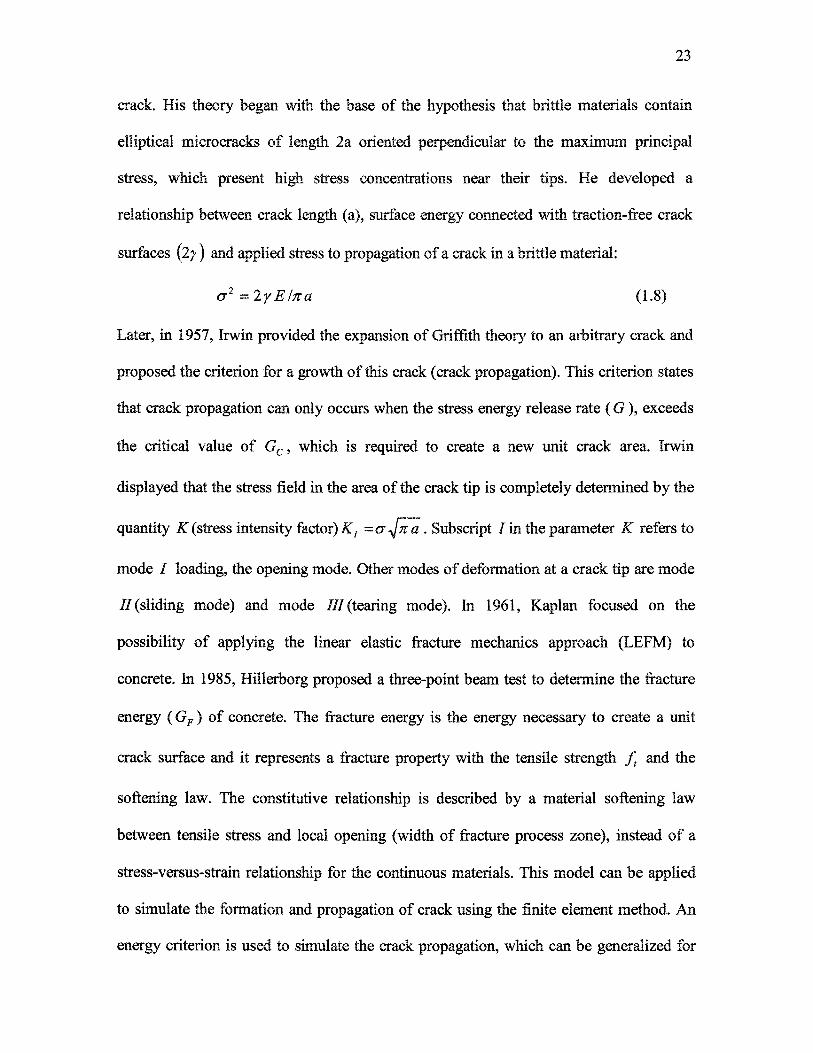
crack. His theory began with the base of the hypothesis that brittle materials contain
elliptical microcracks of length 2a oriented perpendicular to the maximum principal
stress, which present high stress concentrations near their tips. He developed a
relationship between crack length (a), surface energy connected with traction-free crack
surfaces (if ) and applied stress to propagation of a crack in a brittle material:
(j%=2yEina (1.8)
Later, in 1957, Irwin provided the expansion of Griffith theory to an arbitrary crack and
proposed the criterion for a growth of this crack (crack propagation). This criterion states
that crack propagation can only occurs when the stress energy release rate ( G ), exceeds
the critical value of Gc, which is required to create a new unit crack area. Irwin
displayed that the stress field in the area of the crack tip is completely determined by the
quantity K (stress intensity factor)K, =a-^rca . Subscript / in the parameter K refers to
mode / loading, the opening mode. Other modes of deformation at a crack tip are mode
//(sliding mode) and mode ///(tearing mode). In 1961, Kaplan focused on the
possibility of applying the linear elastic fracture mechanics approach (LEFM) to
concrete. In 1985, Hillerborg proposed a three-point beam test to determine the fracture
energy ( GF ) of concrete. The fracture energy is the energy necessary to create a unit
crack surface and it represents a fracture property with the tensile strength ft and the
softening law. The constitutive relationship is described by a material softening law
between tensile stress and local opening (width of fracture process zone), instead of a
stress-versus-strain relationship for the continuous materials. This model can be applied
to simulate the formation and propagation of crack using the finite element method. An
energy criterion is used to simulate the crack propagation, which can be generalized for

24
non-linear materials behaviour. This model is especially suitable for finite element
analysis (see Chapter 3).
1.4 Objectives
The main objectives of the planned research work are:
1) To develop a 3D numerical model to simulate the de-icing of an aluminium structure.
2) To study mechanisms of interaction between ice and substrate using the hypothesis of
fracture propagation criteria and models that could explain these observations.
3) To compare the simulation results with the experimental results obtained from tests in
the AMIL laboratory, and draw conclusions regarding the accuracy of the models.
The primary objective is to study the mechanical behaviour of the interface between
ice (in the brittle region) and substrate to improve mechanical de-icing techniques. To
obtain the relationship between ice dimensions on interfacial forces between ice and
aluminium in order to develop an accurate model and to ensure its verification, the
various mechanisms and parameters characteristic of the delaminating of the ice will be
studied. To do so, the realistic behaviour of the ice, as well as the geometry of the
components and the mechanisms occurring at the interface must be considered.
The ultimate goal of this project is to develop a three-dimensional finite element
model to simulate the de-icing aluminium structure. This could correctly represent the
behaviour of the interface between ice and aluminium. For this, besides the required data
from literature, some systematic experimental tests are necessary, e.g to determine the

25
required supporting experimental data for modeling a traction test. Also, for fitting
reliable interaction parameters, some data must be estimated.
1.5 Methodology
Initially, the proposed methodology consists of establishing a mathematical model
allowing a good representation of the experimental delaminating tensile tests that carried
out within the framework of the doctoral project of C. Laforte, [62].
Firstly, the model will be considered with the simplifying assumptions, such as
linear elasticity of materials. The substrate (aluminium) as well as the ice is supposed to
obey Hook's law. In this way, the effect of adhesion and cohesion between the ice and
the substrate is ignored. From a purely qualitative point of view, it will be worthwhile to
check the influence of the geometrical parameters (width, length, and thickness of the
substrate, thickness and profile of the ice) and materials specifications (Young modulus,
Poisson's ratio) on the shear stress distribution at the interface.
Then, modeling will be carried out finely, and the effect of adhesion and friction
between the ice and the substrate will be taken into account using cohesive material
theory; the nonlinear behaviour of the ice and the substrate will be considered. Certain
constitutive laws make it possible to take into account the energy dissipated by the
mechanisms of cohesion and friction at a total assessment [27]. Also, the constitutive law
for the ice, taking into account the distinct behaviour in traction and compression with
cracking, must be planned in order to adequately capture the risks of cracking before
delamination, as the unknown parameters of these laws will be obtained by retro-

26
engineering with the experimental results.Then it will be possible to quantify the energy
that is mobilized by the interface during delamination.
The proposed approach provides a framework for ice using appropriate progressive
failure analyses where delamination is present. The approach consists of using interfacial
decohesion formulation between the ice and an aluminium plate. The constitutive
equations for the interface consist of mechanical relations between the tractions and
interfacial separations. When the interfacial separation increases, the tractions across the
interface reach a maximum decrease, and vanish when complete decohesion occurs. The
work of normal and tangential separation can be related to the critical values of energy
release rate, G [7].
ABAQUS, a general purpose finite element software, has been selected as the basic
platform for this study. ABAQUS has a unique procedure for attaining solutions for
interface using cohesive material: the unique ability to simulate delamination and de-
icing. In order to predict the initiation and growth of delamination, an eight-node
decohesion element is developed and implemented in the ABAQUS finite element code
[1]. The decohesion element is used to model the interface between two layers, or
between two bonded components. The material response makes it possible for the
element to represent damage using a cohesive zone ahead of the crack tip to predict
delamination growth.
To analyse the delamination growth using decohesion formulation, a fracture
mechanics approach and evaluating the components of the energy release rate G, is
applied. The energy release rate G values are usually evaluated using the virtual crack
closure technique (VCCT) proposed by Rybicki and Kanninen [57]. The approach is

27
computationally effective because the components of the energy release rate can be
obtained from only one analysis.
Decohesion formulations are specified on the basis of a Dudgale-Barenblatt
cohesive zone approach [10 and 29], which is related to Griffith's theory of fracture when
the cohesive zone size is negligible compared with characteristic dimensions, regardless
of the shape of the constitutive equation [19]. These decohesion formulation use failure
criteria that combine aspects of strength-based analysis to predict the softening process at
the interface and fracture mechanics to predict delamination propagation. A main
advantage of using cohesive elements is that without previous knowledge of the crack
location and propagation direction, both onset and propagation of delamination can be
predicted.
1.6 Overview of the thesis
This research introduces and discusses a finite element model that predicts the
initiation and growth of delamination of ice/aluminium using decohesion formulation to
model the interface between ice and aluminium (de-icing). The following is the summery
of the contents of various chapters presented in this thesis:
Chapter 1 introduces the problem of ice in cold regions and also provides a brief
review of the literature. In addition, the necessity of the research, the general objectives,
and the methodology are outlined briefly in those sections.
Chapter 2 presents the laboratory experiments. Such experiments were carried out
with different thicknesses of ice. The ice-making method and conditions are explained in

28
this chapter. The data from these experiments will be modeled by the ABAQUS codes for
comparison with numerical model and for the validation of computer codes.
Chapter 3 presents the mathematical model and also contains a discussion of the
cohesive material theory and the thought that went into the use of cohesive material to
define the interfacial forces and brittle cracking constitutive low to define the brittle
failure of ice. Also, it explains how the cohesive elements are used to show how this
method can support the analysis and presentation of data.
Chapter 4 presents the linear and nonlinear approach. Also, this chapter concludes
with some comments and the results of some simulations performed under three different
thickness of ice.
Chapter 5 contains the important conclusion and the main observations of the thesis
are made in this chapter. This chapter ends by hinting at the scope and the possible
directions for further work.

CHAPTER 2
EXPERIMENTAL TESTS

30
CHAPTER 2
EXPERIMENTAL TESTS
2.1 General
The mechanical properties of structural materials are normally determined by tests
which subject the specimen to comparatively simple stress conditions. For example, most
of our information concerning the strength of material has been obtained from tensile
tests. In a tensile experiment, the specimen is gripped firmly by mechanical jaws at the
wide portion on either side and extended by means of a tensile testing machine. The
pulling is normally carried out at different rates, depending on the type of material being
tested. The low speeds are used to test rigid materials, and the higher speeds are chosen to
test flexible materials. In this research, the tensile tests of ice accumulated on aluminium
plates were carried out in order to introduce a model finite element that predicts the
initiation and growth of delamination of ice/aluminium.
2.2 Sample preparation and icing
In order to have repeatable and comparable tests, all tests must be accomplished
under suitably controlled conditions. Controlled conditions include the use of an
appropriate cooling system (temperature), wind velocity (air circulation), water spraying

31
system and ice thickness deposited on an aluminium plate. Table 2.1 shows the
experimental conditions of ice samples. In this study, the fine granular ice deposited on
the aluminium plate was fabricated by spraying very fine water mist at -10 °C in one cold
room at the AMIL laboratory. The water mist dropped on the surface of an aluminium
plate which was firmly clamped by the mechanical jaws of the tensile test machine and
quickly frozen to form a fine granular ice layer. Before the icing, the aluminium plate
was elongated by approximately 0.05%. In this manner, the aluminium plate was
perfectly horizontal and the ice accumulated uniformly. The length of the aluminium
plate was 168 mm, and the width and the thickness of the plate were 18.87 mm and 0.43
mm, respectively.
Briefly, the method used to make ice with small crystal grains on aluminium
substrate consisted of the following steps:
1) Suitable meteorological factors such as wind velocity and droplet size were controlled
by using suitable air and water pressure, determined by trial and error, in the climate
room. This room had been equipped with a water droplet generator (nozzle) and a
cooling system with the accuracy of temperature control equal 0.1 °C. The
environmental temperature was adjusted to -10 °C during the ice accretion period and
the performance of the tests.
2) High purity water (ASTM deionized distilled water D1193) was sprayed onto a
cooled aluminium plate which was already held in a tensile test machine in the cold
room to form a thin layer of ice.
3) The procedure was repeated to get the desired thickness of the ice sample. The grain
size of ice samples made by this method was typically 1 mm.

32
The ice-making temperature was an important variable in these experiments, and
the aluminium plate was held at the selected temperature (-10 °C) in the cold room for at
least 1 hour before the ice-making process began. Then, the hydraulic water spray nozzle,
fed with distilled and deionized water (ASTM deionized distilled water Dl 193), starts to
spray super-cooled droplets. The water then dropped on the surface of the aluminium
substrate and froze quickly to form a granular ice layer. The time required to make the ice
samples varied according to the temperature and ice thickness, so the icing is stopped
when the aluminium sample is covered with the desired thickness of ice. Each specimen
was kept at the ice-making temperature for one hour before starting the test process. This
time allows the internal stresses to relax before testing, so that no temperature
disturbances appear at this juncture. After this time, the ice is strongly bonded to the
aluminium plate. The experimental protocol and more details are presented in Appendix
D.
Table 2.1: The experimental conditions
Parameters
Type of precipitations
Water temperature, Tw
Air temperature, Ta
Type of water
Jet edge
Time of spray nozzle
Ventilator
Intensity of precipitations
Units
°C
°c
sec
Hz
mm/à
of ice samples.
Type -quantity
Rain glaze
= 4
-10 .010 .5
Deionized
11001
For opening = 0.4
For stopping = 0.9
40
18

33
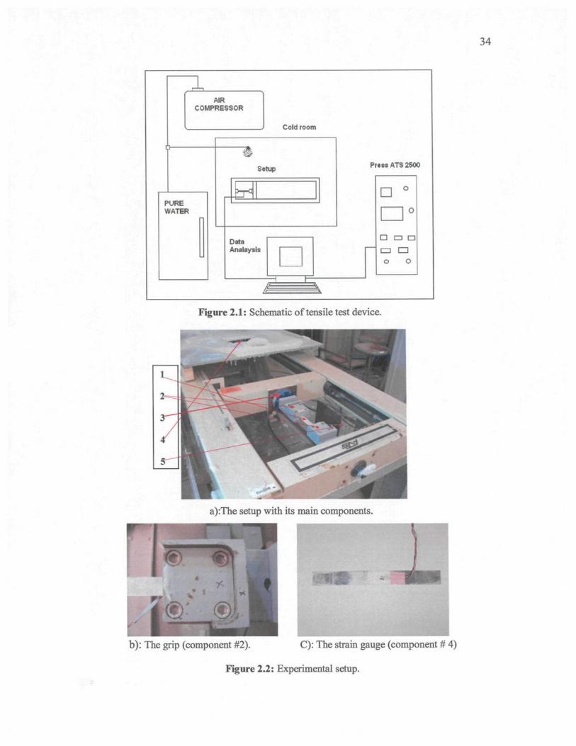
2.3 The setup
Figures 2.1 and 2.2 show a schematic and a photograph of the test device,
respectively. The experimental setup consists of a press machine model Applied Test
system, ATS 2500 which is placed horizontally in the cold room. The sample must be
directly under the jets of freezing ice. The main components of the experimental setup for
the traction test are illustrated in Figure 2.2. The main components of experimental setup
in this figure are: the aluminium plate that is used as the ice-coated beam sample after ice
accumulate (#1) which is mounted in the grips of the testing machine (# 2, see also
Figure 2.2 (b)) and subjected to centric tensile loading (# 3), applied steadily at constant
rate of 0.05921 mm/s (M7 position of press machine ATS 2500) at a cold room with -
10°C. A mould (# 4) is installed before icing to permit the accumulation of ice on the
sample's surface only. A strain gauge (# 5, see also Figure 2.2 (c)) is attached to the back
face of the sample, and the PC software Quick log starts to read the values of strain in a
real time from the strain gauge. The testing procedure consists of applying successive
increments of load while taking the corresponding extensometer reading of the elongation
between two gauge marks on the sample. Also, a high speed camera (500 images per
second) was used for the visual observation of cracking and de-icing.
34
AIRCOMPRESSOR
Cold room
PUREWATER
"ASetup Pt«*6 ATS 2500
DataAnalaysis
ë
� o nen �o o
Figure 2.1: Schematic of tensile test device.
a):The setup with its main components.
b): The grip (component #2). C): The strain gauge (component # 4)
Figure 2.2: Experimental setup.

35
Strain gauges are used to determine the state of strain existing at a point on a loaded
member for the purpose of stress analysis. The strain is the change in a dimension
brought about by load application, divided by the initial dimension, as shown in Figure
2.3:
L -L,(2.1)
The tensile stress is measured as the force at any time divided by the original cross-
sectional area of the waist portion in NI m1, i.e.:
force recorded at any timeoriginal waist cross sectional area
The tensile strain is calculated as the ratio of the difference in length between the length
marked by the gauge marks and the original length, i.e.
-, ., . Gauge length after extensionTensile strain = -
Original gauge length
SubstratIce
Figure 2.3: Relations for axial and lateral strains.
The related equations to determine the value of strain at failure for ice are presented
in Table 2.2. In order to validate the measure of strain, firstly, it is assumed that just
before the fracture of ice the value of strain in ice and aluminium are the same. In this

36
assumption, the measured value of strain for the uncovered part at each end of the
substrate can be representative of that prevailing in the ice just before ice separation. The
validity of this assumption depends mainly on the quality of the adhesion at the interface
between the two materials. Here, it is assumed that the two materials are bonded
completely. Secondly, it is assumed that the strain values remain constant throughout the
length of ice-coated sample. Therefore, the measured strain during a tensile test can be
represented by that being exerted in the middle of the sample (where the strain gage is
located).
Using the relations for uniaxial condition such as they exist in a simple tensile test
specimen, the complete stress-strain diagram can be determined for the material as
described in Figures 2.4 to 2.6 for each thickness of ice. In these Figures, the dotted curve
in dark blue is the average applied stress in function of the strain of the ice-coated
sample. The strain values in the x axes are measured directly by the strain gauge, whereas
the applied stress values in the Y axes are the applied load measured in the traction test
divided by the section area of the aluminium plate. Generally, ice accumulation increases
rigidity, because the deposit of ice increases the thickness. When the ice breaks or de-
icing is occurred the rigidity decreases. This decreasing of rigidity appears with the
change of the slope of graph. The slope can be changed gradually (Figure 2.4) or
discontinuously with a jump (Figure 2.6). A gradual change of slope is interpreted as de-
icing (ice removal) occurs slowly or there is simply ice breaking without de-icing. The
break in slope is interpreted as ice removal (de-icing) occurs very fast.

37
Table 2.2: The related equations to determine the stress values.
Calculated Values
"no rain a/ 7 Ob
E
G ice fract.
Equations
"subsl. *subsl.
E = <*>** measured
If Sice=£^borate
&ice fract. ~ &pact ^g
Parameters (Unite)
P = applied force (kg)g=9.82(m/s ï)
b subst. - width of substrate (m)hubst. ~ thickness of substrate (m)
<TnDminflf= nominal stress (MPa)
Smtawreti ^measured strain by gage
Eg= 9000 (MPa)
G(ract= strain at fracture
� Deformation � Young modulus without ice x Young modulus with ice
180.00
0.000000 0.000500 0.001000 0.001500
Strain [mm/mm]
0.002000
0.00
0.002500
Figure 2.4: Experimental stress� strain curve for ice thickness 2 mm (test 1).

38
� Deformation � Young modulus without ice x Young modulus with ice
160.00
140.00
120.00
reQ.
100.00 t i
80.00
60.00
40.00
20.00
0.000.000000 0.000500 0.001000 0.001500 0.002000 0.002500
Strain [mm]
O
(A
Figure 2.5: Experimental stress- strain curve for ice thickness 5 mm (test 6).

39
� Deformation �Young modulus without ice x Young modulus with ice
180
160
140
120
D- 100
£ 80CO
60
40 -
20
x *
XX *
180,00
� 160,00
� 140,00
� 120,00 n
Q.CD0
� � 100,00 . 2
- 80,00 iff
60,00 >"
� 40,00
- 20,00
0,000,000000 0,000500 0,001000 0,001500 0,002000 0,002500
Strain [mm/mm]
Figure 2.6: Experimental stress- strain curve for ice thickness 10 mm (test 9).
2.4 Test results and discussions
For each different thickness of ice, three tests were performed under the same
conditions. The results of these tests show that:

40
1) In the case of the 2 mm thickness, the tensile stress imposed at the ice sheet generates
the cracks perpendicular to the aluminium length, breaking it in pieces (see Figure
2.7 and ice failure is characteristic of a brittle failure. This mode of failure is
expected, given the very fast deformation rate imposed, which is equal to a strain rate
of about 2 x 1(T4 mm/s. Also, the experiments show that when water is frozen on an
aluminium surface which is completely wet, the interfacial forces for a thin thickness
of ice are larger than the cohesive forces of the ice. For this reason, when the sample
is stressed, the failure occurs in the ice; however, the form of the failure depends on
the experimental configuration. If the ice is suitably constrained, if the tensile forces
are spread over a large enough area so that the tensile stresses are small, the ice
deforms plastically, the breaking force is proportional to the number of degrees of
frost, and if the tensile stress is large compared with the shear forces (as our tests), a
brittle fracture takes place and the breaking force is dependent on the thickness of
ice. The results show that with the thickness of ice equalling 2 mm, the interface is
stronger than the ice and cracks are created in the ice sheet. In other words,
corresponding to a thin thickness of ice, the surface molecules are more susceptible
to breakage than bulk and interface molecules, which means in this case the cohesive
failure (Failure occurs within ice itself) is more probable than adhesive failure
(failure of the bond between the adhesive and substrate surface).

41
a): Ice-coated beam sample before testing. b): Ice-coated beam sample after testing.
Figure 2.7: Description of the tensile test.
2) hi the case of the 5 mm thickness, it can be observed that not only ice fracture
(cohesive failure) but also ice removal (adhesive failure) occurs. In this case, a
transition is observed from cohesive to adhesive failure, and a significant proportion
of specimens exhibited some regions of interfacial separation in this thickness range.
3) In the case of the 10 mm thickness, ice de-bonds without breaking the ice sheet
(cohesive break). In this case, the ice is stronger than the interface and ice removal
occurs without cracking the ice. hi other words, the crack extended along the
interface and the bonding was broken by an adhesive separation. The results obtained
in these nine tests are presented in Table 2.3. Also, the force versus strain graphs for
tests number 2, 6 and 9 are shown in Figures 2.8, 2.9 and 2.10 respectively (the
results from these three tests will be used for the numerical model).

42
Table 2.3: Tensile test data.
Test
123456789
Ice thickness(mm)
2.611.973.296.595.565.359.9810.0910.09
Strain(mm/mm)
0.0005080.0005290.0005700.000520.000400.0005030.0002990.0003540.000375
Force(N)
340.01343.35369.83373.27310.97329.20372.87348.25297.63
Normal stressat bottom facein Al (MPa)
35.5637.0339.936.428.035.2120.9324.7826.25
600
500 -
400 -
S 300
200 -
100 -
00 0.0002 0.0004 0.0006 0.0008 0.001 0.0012
Strain [mmftnm]
Figure 2.8: Experimental force - strain curve for ice thickness 2 mm.
1 1 ' I �
343.34
i.
i.
i.
i �
/
0.000529
i '
i
i i
-
.I
.I
.I

43
S»
u u u
500
400
300
200
100
n
i
-
-
� 329.20
-
� *
* ^ * . i
i � i � i
i
-
-
O.OOO5O3I . I .
0 0.0002 0.0004 0.0006 0.0008 0.001
Strain [mmfrnm]
Figure 2.9: Experimental force - strain curve for ice thickness 5 mm.
600
500 -
8
400 -
300
200 -
100 -
-
297.63
I.
I.
T" . I .
1
0.000375i ,
I.
I.
I . I .
0 0.0002 0.0004 0.0006 0.0008 0.001
Strain [mmlrn]
Figure 2.10: Experimental force - strain curve for ice thickness 10 mm.

CHAPTER 3
THEORY AND MATHEMATICAL MODELFOR ICE AND INTERFACE

45
CHAPTER 3
THEORY AND MATHEMATICAL MODEL
FOR ICE AND INTERFACE
3.1 General
Mathematical modeling can be used to represent some phenomena in order to gain
a better understanding of that phenomenon by exhibiting a designated similarity to
physical objects. A mathematical model attempts to match observation that uses
mathematical equations. When a model is developed and it is used to answer questions, it
should be examined, and often modified, to obtain a more accurate response of the
observed reality of that phenomenon. In this way, mathematical modeling is a developing
process, and each real-world phenomenon can be represented by using theoretical,
mathematical, and computational models together, hi order to describe the stress-strain
behaviour of ice on the substrate under tension loading, a model will be developed to
improve our understanding of the mechanisms of ice/substrate interface underlying the
mechanical properties of ice. This chapter first presents a mathematical model based on
classical beam theory, and then describes the two proposed constitutive laws for ice and
interface in detail, respectively: a brittle cracking constitutive law, which has been
developed basically for concrete and can be used for the other brittle materials such as

46
ice, and a cohesive material constitutive law which predicts the initiation as well as
evolution of damage to the interface.
3.2 The classical linear beam theory
In order to define a simplified mathematical model, the ice mass on the aluminium
plate can be assumed to be a composite material. Using the elastic properties of each
material, the equations are defined considering an equivalent material. The free-body
diagram of the model is shown in Figure 3.1. From this theory, we can develop the
following relations.
b)
c)
Figure 3.1: Free-body diagram of the theoretical model, a) Description of the geometry,b) Description of section A-A, c) Equilibrium of the beam system.

47
A formula for normal stress is [98]:
°.=-f 0.1)where M and / are the bending moment and the moment of inertia respectively. Usually
called the elastic bending formula, this important equation shows that the stresses vary
linearly with the distance (y) from the neutral axis. For combined normal force and
bending, the axial stress is given by:
(3-2)x A I
The maximum stress o rtsaL occurs at the outermost fibres of the beam. Since at a given
section, M and / are constant,
_Mc _M<7�-~r-~S (3.3)
where c = \ynwi , and S = � is called the elastic section modulus of the beam. For a beamc
of rectangular cross section with width b and height h, we have:
bhl btf_z 12 6
The substrate covered by ice can be assumed to be a composite material. The materials
having different modules of elasticity must be combined as unique materials with the
balance coefficient ( n ) such that:
n = � (3.5)
If Iice and Ia1 represent the moments of inertia about the neutral axis of the cross-
sectional areas ice (Alce) and aluminium (Aal), respectively, it is convenient to define a
combined inertia and total area given by:

48
I1 =Iice+nIa!,
A' =Aice+nAal
The flexure formulas now are given by:
(3.6)
(3.7)
A,- * (3.8)
where cr*e and <r° are the stresses in materials ice and aluminium, respectively.
In the iced composite beam solicited in flexion by a bending moment
M -forcexeccentricity, the value of shear stress t at the aluminium interface can be
calculated from the applied shear force V. The value of shear flux due to the variation of
the bending moment (see Figure 3.1(c) and 3.2) is given by:
Qyxv
Figure 3.2: Description of shear flux due to the variation of the bending moment.
(3.9)
where
V = -dM
dx(3.10)
and
= t bice feel 2
(3.11)

And from equilibrium at interface:
49
(3.12)
x
P
Nice+Nai=N
Figure 3.3: Description of equivalent shear flux.
Considering the assumption that the equivalent shear flux is uniform on the mid-length:
il (3.13)
and the values of shear stress t at ice and aluminium interfaces are given respectively
by:
qyx
n(3.14)

50
Equations 3.1 to 3.14 have been implemented in the numerical software Maple to
determine the normal stress and shear stress distribution in accordance to the linear
elastic theory. Figure 3.4 shows the normal stress distribution at mid-length for the three
thicknesses of ice considered in the experimental setup and for an external applied force
corresponding to the point of fracture as shown in Figures 2.8 to 2.10.
en
�0 S 0.5
Distance over the thickness [mm]
\
Al
uy1In
te
30-
25-
20'
15-
10-
.1
FMIce
� »
Distance over the thickness [mm]
Al
u
k
� 4
20
16-
10
5
� ' � � i ' ' ' «
Distance over
[MPa
]
M
- ! " �
the thickness [mm]
b)
Figure 3.4: Normal stress distribution at mid-length for ice thickness: a) 2 mm, b) 5 mm andc) 10 mm.

51
The longitudinal shear stress distributed through the thickness of ice is shown in Figure
3.5:
20 40 60 90 100 120 140 160
Distance through the thickness [mm]
2-
-2-
-1-1
20 «J BO 30 1U0 120 140 160
Distance through the thickness [mm]
b)
S 20 E0 t i f f 140 160
Distance through the thickness [mm]
C)
Figure 3.5: Longitudinal shear stress distribution through the thickness of ice: a) 2 ram, b) 5 mmand c) 10 mm.
In Table 3.1 a comparison between experimental and mathematical models (Maple)
shows that realistic stress distribution cannot be evaluated using the linear description of
the strain tensor. This is mainly due to the small thickness of the aluminium plate. Also,
another argument is that the shear and normal stresses at the interface of the
ice/aluminium have a complex distribution which cannot be demonstrated by using the
classical beam theory. The beam theory also leads one to believe that the interfacial
longitudinal shear stresses can be calculated using the elementary shear stress equations
given in strength of material books (Eq. 3.14). In reality, these stresses have a much more
complex distribution. Furthermore, when the ice on an aluminium plate cracks, the
stresses at the interface in the neighbourhood of the crack deviate significantly from the
distribution predicted by simple beam theory or by any other theory that ignores the

52
presence of cracks. The experimentally observed delamination of ice on aluminium
substrate is caused by the combined effect of these high interfacial stresses.
Table 3.1: Comparative results between the experimental and the mathematical models.
Thickness(mm)
2510
Force(N)
343.35329.20297.63
Normal stress o ^ at bottom
face in Al(MPa)
Experimental37.0335.2126.25
Theoretical43.2732.4422.27
Longitudinal shear stress (Sxz)through the ice
(MPa)
Theoretical4.534.163.62
Experimental*
0.47 ± 0.06
* This average value was obtained from centrifuge test by C. Laforte in LIMA laboratory.
However, there are many theories proposed to understand the complex behaviour of
fracture in the material. One such class of theories, which involved energy concepts, was
developed by Griffith, who recognized that the macroscopic potential energy of the
system consisting of the internal stored elastic energy and the external potential energy of
the applied loads, varied with the size of the crack [95]. Based on the Griffith theory,
fracture is associated with the consumption of energy:
U=U0-Ua-Uy (3.15)
where U is the total potential energy of the system, Uo is the elastic energy of the un-
cracked plate, Ua is the decrease in the elastic energy caused by introducing the crack in
the plate and Uy is the increase in the elastic-surface energy caused by the formation of
the crack surface [95].

53
3.3 Model for the ice
3.3.1 Introduction
The failure mode of ice is dependent on at least four parameters: temperature,
porosity, grain size and strain rate. Here, it is focused on the strain rate effects, because
our experimental tests were performed at a high strain rate. The scope of the problem is
that a brittle failure mode will occur when the strain rate is higher than IO~3 s'1 and a
ductile failure mode will dominate when the strain rate is lower than KT3.?"1 [25]. At
strain rates below lO""5^"1 in tension and 10"4*"1 in compression, ice deforms mostly by
creep. At higher strain rates, ice deformation is mostly elastic because it takes time to
develop creep deformation, and the failure of ice specimens is by fracture [25]. Figure 3.6
shows the schematic effect of strain rate on the tensile and compressive stress-strain
behaviour of ice. At low rates of deformation, cracks do not form, and the material has a
ductile behaviour (Figure 3.6 - curves I). At high rates, cracks do initiate, and the material
has a brittle behaviour (Figure 3.6 - curves III) independent of stress state. At
intermediate strain rates, cracks also develop, and the behaviour of material is brittle
under tension (Figure 3.6 - curve Til) but ductile under compression (Figure 3.6 - curve
CII). At lower strain rates the ductile-brittle transition occurs under tension because the
applied stress opens the cracks directly [83]. Figure 3.7 shows the tensile and
compressive strengths of fresh-water ice of about 1 mm in grain size versus strain rate
loaded uniaxially at temperatures around -10°C. For ice deformed under these conditions,
the low strain rate is less than lO"7^"1 and the high strain rate is greater than KTV 1 [83].

54
uCO
I
rTension
II
A/i
Compression
II A
Axial Strain
Figure 3.6: Schematic effect of strain rate on the tensile andcompressive stress-strain behaviour of ice. I, II, and III denote low-,intermediate-, and high-strain rates respectively [83].
Ou
fiKl«
J.2S
10
9
e
7
8
5
4
3
2
1
Sym. Load. T (°C) References
� T -10O » c -10A c -10O C -7
0 4 c -11.8
Lee(1985)
Schulson(1990)
Schulson & Cannon (1984)
Hawkes&Mellor(1972)
Jones(1982)
1tf i or;f;WflB
10"* 10"* 10"4 1Axial strain rate (S"1)
T"n i
10',-t
Figure 3.7: Graph demonstrating the effect of strain rate on the uniaxialcompressive strength (C) of equiaxed and randomly oriented polycrystalsof ice Di of 1 mm grain size at -10°C. The tensile strength (T) is shown forcomparison. The peak in the compressive strength versus strain rate marksthe macroscopic ductile-to-brittle transition [83].

55
In the range of the average loading rate in our experiments (» lO^s"1), ice has a brittle
behaviour. This behaviour will be explained in this section.
The most commonly-used method to calculate stresses from a structural engineer's
point of view is the theories from strength of materials. The mechanical engineer is able
to look at the microstructure of the failure process, and if there are cracks in the failure
one may try to use the linear elastic fracture mechanics (LEFM) approach. This approach
will be illustrated in this section in order to describe the parameters, the critical stress
intensity factor i£/c, and the energy release rate G for using a brittle cracking ice model.
3.3.2 Brittle behaviour of ice under tension
At higher strain rates under tension (regimes Til & Till, Figures 3.6 and 3.7) ice
breaks after lengthening 0.01-0.1% through transgranular cleavage, at an applied stress
around 1 MPa [23, 42, 72, 84 and 85]. As described in section 1.3.2, the tensile strength
of ice is essentially rate independent and slightly dependent on temperature, increasing by
less than 25% upon decreasing temperature from -5°C to -20°C. Also, the tensile strength
decreases with increasing grain size [83]. The tensile behaviour of ice has been described
and modeled in the nucleation and growth of cracks (propagation) terms. Their resistance
to propagation is controlled by the fracture toughness of the material. Therefore, within
finely grained size (around 1-2 mm), cracks are shorter upon nucleation than the critical
size, so the tensile strength is limited by crack propagation. With more coarsely-grained
ice, the cracks propagate immediately based on nucleation. The significance is that the
tensile strength of the cracked ice is controlled by crack propagation [85]. Apart from
cracks, grain size has the largest effect on tensile strength of ice. For example, by

56
decreasing the grain diameter d from 10 to lmm, the strength ot increases by about a
factor of 2 as illustrated in Figures 3.8 (b) and 3.8 (c).
0.8Grain size ~y 2 (mm ~v 2)
Crack propagation
0.2 0.4
Grain size
0.80.6
'(mm1")
Figure 3.8: Graphs of tensile fracture stress versus (grain size)"0'5 of equiaxed andrandomly-oriented aggregates of fresh-water ice Ih loaded under uniaxial tension: a)showing schematically the critical grain size, dc, below which the material exhibitsa minor amount of inelastic deformation that increases with decreasing grain size; b)
showing that at -10°C at a strain rate of lO"3^"1, where dc <1.4 mm, the strength iscontrolled by crack nucleation; and c) showing that at -10°C at a strain rate of
10" 5~ , where dc) 6.7 mm, the strength is controlled by crack propagation [87].
The relationship is either [87]:
(ford>dc) (3.16)
or

57
cr, = Kd^5 (ford < dc) (3.17)
where ao, kt and Ã"are material constants and dc\s critical grain size. Values at -10°C
are <ro = 0.6 MPa, kt= 0.02 MPaVm and K= 0.044 MPaV/n , with increasing strain
rate, dc decreases from > 6.7 mm at 10 "7 S "* to 1.6 mm at 10 "6 S -1 and to < 1.4 mm at
10'3 S A [85 and 86]. According to the concept of brittle fracture and the mechanisms
underlying Equations (3.16) and (3.17), critical grain size dc, is given by :
°"o
3.3.3 The brittle cracking theory
The cracking constitutive model for ice and other brittle materials is described in
this section. As aforementioned, it is generally accepted that ice exhibits two primary
modes of behaviour:
1) A brittle mode that is associated with cleavage, shear and mixed-mode fracture
mechanisms that are observed under tension and tension-compression states of stress.
It almost always involves softening of the material.
2) A ductile mode that is associated with distributed microcracking mechanisms that are
primarily observed under compression states of stress. It almost always involves
hardening of the material.
The cracking model that is described here models only the brittle aspects of ice
behaviour. The brittle cracking model is used for applications in which the material
behaviour is dominated by tensile cracking and compressive failure is unimportant.

58
3.3.3.1 Fracture mechanics of brittle materials based on linear elastic fracture mechanic
(LEFM)
As described briefly in section 1.3.4 (a history of fracture mechanics of brittle
materials) in LEFM, crack growth is defined by the energy release rate G and stress
intensity factor Kj (index I related to mode I). To define these variables, a crack of length
2a, which extends right through an infinite elastic flat plate with dimension D and small
thickness b (see Figure 3.9) is considered. From equilibrium, compatibility and the linear
elastic constitutive law (the material is assumed as linear elastic), the stress distribution in
the uncracked part of the panel is [13]:
°"22 = °nx,
(3.19)
tttt'MMt,
Figure 3.9: Multiaxial stressed panel with thickness b andwidth D, and a predefined crack width 2a [13].
If we then let the distance xx -a {{a, then the stress intensity factor, K, which defines the
magnitude of the local stresses around the crack tip as:

59
(3.20)
This intensity factor depends on loading, crack shape, crack size, and geometric
boundaries. The stress distribution in the intact panel is given by:
^ 2 2 = ! = (3-21)
where r is equal to x, - a .
To define the energy release rate parameter G, the relation between the energy
release rate and the stress intensity factor K} is called Irwin's formula, and derivations
are shown in many fracture mechanics textbooks [13]. Here we only consider the result
of the derivations; the famous Irwin's formula is:
G = - (3.22)
where E is the elastic modulus.
Let us now turn to the local crack growth in Mode I. Since intensity factor K1 only
determines the stress state of the material in the crack tip (a very small fracture process
zone), the crack will propagate when this stress intensity factor reaches a critical
value, Klc, called fracture toughness [3]. According to the fundamental relationship (Eq.
3.22), KIc is related to the fracture energy by:
(3.23)
where the index / on G will be used when the fracture is considered.
It is quite hard to get a good value of Klc for ice. The typical values of K]c are in the
range of 80 - 120 kPa m'2 for pure ice. The mean values obtained by different authors

60
for the critical stress intensity factor Klc and corresponding Gf values are presented in
Table 3.2. In Appendix A, the mixed-mode bending (MMB) test is analyzed using beam
theory to calculate the mode I and mode II components of strain energy release rate, G7
and Gu respectively.
Table 3.2: Fracture toughness and critical stress intensity factor for ice [96].
Authors
Goodman
Goodman andTabor(1978)Liu and Miller(1979)Gold (1963)
TemperatureT°C
-11
-13
�
-16.7
Critical stress intensityfactor KIC
KN.m^2
119 ± 34
116 ± 13
108 ± 10
94-110
Fracture toughnessG
Jrrf2 or �m
1.45 ± 0.83
1.41+ 0.31
1.471 ± 0.27
0.923-1.53
3.3.3.2 Determining the fracture energy of interfaces
The fracture mechanics approach is ideally suited to the interfacial failure subjects,
and has interested many researchers in mechanics and materials science [30, 47, 49, 76,
79, 94 and 99]. In the last decade, interface fracture mechanics has been the object of
significant development and which can be applied to the ice/solid interface adhesion
problem. It should be noted that the crack growth of bi-material interface cracks like
ice/solid interface is always mixed-mode because of the mismatch of material properties
across the interface. The fracture of bi-material interfaces can be characterized by two
parameters: the fracture energy Gf, and the phase angle y/ [30]. As aforementioned, the
fracture energy Gf can be obtained via the energy release rate calibration of test

61
specimens or can be calculated from the critical stress intensity factor KIC (Eq. 3.23).
The phase angle y is a measure of the mixity of shear-to-opening experienced by an
interface crack surface, and can be determined either from finite element calculations or
by using integral equation methods. The sign and magnitude of y are of particular
significance in determining whether a propagating crack can extend along the interface or
kink into one of the composite constituents [101]. Obviously, performing standard shear,
tensile, or impact tests is not sufficient to characterize the failure of ice/solid interfaces.
This work attempts to utilize fracture mechanics to characterize the failure of
ice/aluminium adhesion.
Various methods exist to characterize the fracture energy of interfaces [30].
Charalambides et al developed a four-point bending delamination specimen (see Figure
3.10) to determine the critical energy release rate at the bimaterial interface. The method
of Charalambides et al. has the advantage of being able to simulate icing on the surface
of structures on the simple sample geometry. This method has been described in
Appendix c.
P/2b
i
Figure 3.10: Four-point bending specimen geometry and loading configuration.

62
The phase angle y of this configuration is in the range of 35°- 60° [47]. This method
was used by Wei et al [101], in order to characterize the failure of ice/solid adhesion. On
the base of the Euler-Bernoulli beam theory, the critical interface fracture energy Gf is:
_M]{\-vl) I xf IE, V, I
(3.24)
where
Mf= � ,I2=!2- (3.25)
The bending moment Mf exists along the sample cross section. / denotes the moment of
inertia, the subscripts 1 and 2 refer to the ice and substrate materials respectively, and
subscript c refers to the composite beam. It should be noted that this approach is valid
when the crack length must be significantly larger than the thickness of the upper layer.
Table 3.3 gives the values of fracture energy for different ice/metal interfaces tested by
Wei et al. [101].
Table 3.3: Fracture energy of ice/metal interfaces (a/1 = 0.5) [101].
Interface type
Ice/AlIce/steel
Relative thickness
KK0.81.0
Relative modulusE2
Ex
7.120.4
Fracture energy Gf
(Jm~2 or �)m
1.01.1
Analytical results [22] show that the fracture energy Gf increases monotonically
when the relative upper beam thickness hx jh2 increases and decreases when the relative
modulus of the lower layer E2 /Ex increases. Also, it should be noted that the fracture

63
energy of ice/metal interfaces is affected by the ice type and the procedure of ice
formation on substrate [101].
3.3.3.3 Analysis of crack formation and crack growth in ice
Recently, the development of finite element methods (FEM) and fracture
mechanics have now given us the possibility of analysing crack growth. While the
fundamental rules for crack propagation come from the fracture mechanics approach (e.g.
the energy balance approach), FEM makes it possible to apply these rules to complicated
cases.
As aforementioned, in the energy balance approach it is assumed that a certain
amount of energy, Gf, is absorbed by the formation of a unit area of the crack surface.
The crack propagates when a certain amount of stored energy is released and this released
energy is equal to or greater than the absorbed energy. FEM can be used to determine the
energy release rate in the energy balance approach. This enables the use of a FEM mesh
with rather large elements. The formation of cracks cannot be explained with this energy
balance approach [44].
The crack is assumed to propagate when the stress at the crack tip reaches the
tensile strength ft. When the crack opens, the stress is not assumed to fall to zero
immediately, but the stress decreases with increasing crack width 5 . As shown in Figure
3.11 at the crack width Óc, the stress reaches zero. Where 5 <óc, the crack in reality
corresponds to a micro-cracked zone with some remaining ligaments for stress transfer.
As there is a stress to be overcome in opening the crack, energy is absorbed. The amount

64
of energy absorbed per unit crack area in widening the crack from zero to or beyond òc
corresponds to the area between the curve and the coordinate axis in Figure 3.11 is:
(3.26)
Figure 3.11: General case of assumed variation of stresso with crack width Ò .
The o -Ó curve (see Figure 3.11) may be chosen in various shapes, e.g. according to
Figures 3.12 (a), (b) or (c), which all show simple mathematical relations. For typical
yielding materials, like mild steel, Figure 3.12 (a) seems to be the best choice while
Figure 3.12 (c) is the best choice for concrete material [44]. For the ice we consider the
simplest o -Ó curve such as Figure 3.12 (c).
o
o*
a)
O A
b)
Figure 3.12: Typical stress-separation curves.

65
Quantification of the stress-separation model requires knowledge of the shape of the
curve. The shape of the stress-separation curve is important in determining the fracture
process zone development. Typical shapes based on concrete are shown in Figure 3.12.
Pure polycrystalline ice has a much more homogeneous (uniform) microstructure than
concrete; as a result the curve is unlikely to have an elongated tail and the choice of a
linear stress- separation curve (see Figure 3.12 (c)) may be realistic. Identical simplifying
assumptions have been successfully applied to concrete. The critical separation distance
is then given by [44]:
õe=2G,/<r, (3.27)
The value of Gf for ice should be obtained from the area under the stress-
separation curve. In the absence of experimental data for the curve, Gf may be estimated
from Klc values obtained from conventional tests conducted on ice at high loading rates.
3.3.3.4 Using brittle cracking criterion
It is generally accepted that brittle materials such as ice and concrete exhibit two
modes of behaviour:
1) A brittle mode that is related to cleavage, shear and mixed-mode fracture mechanisms
that are observed under tension and tension-compression states of stress.
2) A ductile mode that is associated with distributed microcracking mechanisms that are
primarily observed under compression states of stress. It involves the hardening of
the material.
The brittle cracking theory considers only the brittle aspects of a brittle material.
Although this is a great simplification, there are many cases where only the brittle

66
behaviour of a material is significant, and therefore the assumption that the material is
linear elastic in compression is justified in those cases. Therefore, the brittle cracking
model:
1) Is used for cases in which the behaviour of the brittle material is dominated by tensile
cracking like the behaviour of ice in our tensile test.
2) Assumes that the compressive behaviour of brittle material is always linear elastic.
The cracking behaviour is defined in three parts:
/. Crack directions
The fixed orthogonal cracks model is used with the maximum number of cracks at a
material point limited by the number of direct stress components present at that material
point of the finite element model (for example, a maximum of three cracks in three-
dimensional, axisymmetric, and plane strain problems). Once a crack is created at a point,
the component of all vector and tensor valued quantities are rotated so that they lie in the
local system defined by the crack orientation vectors (the normals to the crack faces). The
model ensures that these crack face normal vectors are orthogonal so that this local
system is the rectangular Cartesian. Crack closing and reopening can take place along the
directions of the crack surface normals. The model neglects any permanent strain
associated with cracking; that is, we assume that the cracks can close completely when
the stress across them becomes compressive [1].
//. Crack detection
In order to detect crack initiation a simple Rankine criterion is used. Based on this
criterion, a crack forms when the maximum principal tensile stress exceeds the tensile
strength of the brittle material. Cracking is not recoverable. This means that once a crack

67
occurred at a point, it remains throughout the rest of calculation. However, crack closing
and reopening may take place along the directions of the crack surface normals. Any
permanent strain associated with cracking is neglected by the model. Therefore, it is
assumed that when the stress across the cracks becomes compressive the cracks can close
completely.
Although crack detection is based on the Mode I fracture, while cracked behaviour
includes both Mode I (tension softening/stiffening) and Mode II (shear
softening/retention) behaviour, details of these two modes will be described later.
///. Cracking conditions
A consistent condition for cracking in the crack direction coordinate system in the
form of a tensor is:
C = c(t,aIJI)=0 (3.28)
where C = [C B n C t t C M C n r C M Cj r
and t = [tm ttt tss tnt tm tts ]T is stress in the local cracking system and <J'M represents a
mode I fracture (tension softening mode) in the case of the direct components of stress
and a mode II fracture (shear softening/retention model) in the case of the shear
components of stress. The matrices ôC/ôt and ôC/ôaIJI are assumed to be diagonal,
implying the assumption that there is no coupling between cracks in the cracking
conditions. Two states of cracking are possible for each cracking condition (an opening
crack state and a closing/reopening crack state). This can be described by writing the
cracking conditions for a particular crack normal direction n (can also be written for the
other two possible crack normal directions, s andí ):

68
O (3.29)
For an opening crack state where crï\ecnkn) is the tension softening evolution and efn is the
crack opening strain and this parameter must be defined by the user. And
Cm=Cm(tnn,cjIc) = tnn -arc(e £
for a closing/reopening crack where
(3.30)
is the crack closing/reopening
evolution. These two conditions are illustrated in Figure 3.13; also, the tension softening
model (mode I) is represented. It should be noted that similar conditions can be written
for the other two possible crack normal directions, s and t.
Figure 3.13: Cracking conditions for Mode I cracking [1].
Also, the shear cracking conditions can be presented, for example, by writing the
conditions for shear component ni (also can be written for the other possible shear
components). Therefore, the crack opening dependent shear model (shear retention
model) is written as:
Cnt=Cnl(tnt,crIJ) = tnt -<TÏ(g5,eî,ef) = 0 (3.31)

69
where as (gcn,,e
cnn,eft ) *s t n e shear evolution that depends linearly on the shear strain
and also depends on the crack opening strain ( efn ) (this parameter also must be defined
by the user). This model is illustrated in Figure 3.14.
ckOnt
<J
Figure 3.14: Cracking conditions for Mode II cracking [1].
Although crack detection is based purely on Mode I fracture considerations,
ensuing cracked behaviour includes both Mode I (tension softening) and Mode II (shear
softening/retention) behaviour, as described:
1) Tension softening/stiffening (mode I):
The basis of the post-cracked behaviour in the direction normal to the crack surface
(tension softening) comes from the brittle fracture concept of Hilleborg [81]. Hilleborg
defines the energy required to open a unit area of crack in Mode I, G'f as a material
parameter, using brittle fracture concepts. This fracture energy can be calculated from
measuring the tensile stress as a function of the crack opening displacement, as follows:
(3.32)

70
As aforementioned, the mode I fracture energy G!f can be specified directly as a material
property; in this case, the failure stress a\ is defined as a tabular function of the mode I
fracture energy. This model assumes a linear loss of strength after cracking (see Figure
3.15).
H.
Figure 3.15: Post-failure stress-fracture energy curve [1].
The crack normal displacement at which complete loss of strength takes place is,
therefore, UnQ = 2G!f I G\ .
2) Shear retention model (mode II):
An important aspect of the cracking model is that, whereas crack initiation is based
on Mode I fracture only, post-cracked behaviour includes Mode II as well as Mode I. The
Mode II shear behaviour depends on the amount of crack opening. The dependency is
when the crack opens, the cracked shear modulus is reduced. Therefore, a shear retention
model can be used in which the post-cracked shear stiffness is defined as a function of the

71
opening strain across the crack. This shear retention model defines the total shear stress
as a function of the total shear strain (shear direction nt is used as an example):
t = Du(pck pck\eck
nt " ^ «íVcnn»l'í/ font(3.33)
where D^t(e fn,ef ) is a stiffness that depends on crack opening, D "t can be expressed
as :
Du = a(eck eck\G (3.34)
where G is the shear modulus of the uncracked material and a (ecm ,ec
tt ) is a user-defined
dependence of the form shown in Figure 3.16.
aTends to infinity
Figure 3.16: Shear retention factor dependence on crack opening [1].
A mathematical form for this dependence when there is only one crack, related to
direction n, is the power law form [5]:

72
1 __ nnck \ P
(3-35)
ckmax
where P and e ^ are material parameters. This form satisfies the requirements that
a �>ooas efn-^>0 (corresponding to the state before crack initiation) and a - »0 as
etn~^etax. (corresponding to complete loss of aggregate integrate). It should be noted
that the bounds of a , as defined in our model using the elastic-cracking strain
decomposition, are ooand zero. This compares with some of the traditional shear
retention models where the intact brittle material and cracking strains are not separated;
in these models the shear retention is defined using a shear retention factor p , which can
have values between one and zero. The relationship between these two shear retention
parameters is:
The shear retention power law form given in Equation 3.35 can then be written in terms
of p as:
ch Y(3-37)

73
Since users are more accustomed to specifying shear retention factors in the traditional
way, (with values between one and zero), the data needed are p � ecnkn data. Using the
above equations, these data are then converted to a - e c*n data for computation purposes.
Therefore, in shear retention models the dependence is defined by expressing the
post-cracking shear modulus Gc, as a fraction of the uncracked shear modulus G :
Gc=p(et)G (3.38)
where the shear retention factor p(e c*n), depends on the crack opening strain, e*. This
dependence can be illustrated in piecewise linear form, as shown in Figure 3.17 [1].
I 1
ck
Figure 3.17: Piecewise linear form of the shear retention model [1].
At least one experiment, a uniaxial tension test, is required to calibrate the simplest
version of the brittle cracking model. Usually, this test is difficult to perform because it is
necessary to have a very stiff testing machine to record the post-cracking response. Quite

74
often such equipment is not available; in this situation we must make an assumption
about the tensile failure strength of the material and the post-cracking response. For ice,
the tensile strength is about 1.4 MPa [83]. Other experiments may be required to gain
accuracy in post-failure behaviour.
Calibration of the post-cracking shear behaviour (mode II) requires combined
tension and shear experiments, which are also difficult to perform. Because such test data
are not available, a value for crack opening strain efn is assumed. It is also assumed that
the shear retention factor p , goes linearly to zero at this crack opening strain.
3.4 Model for the interface
3.4.1 Introduction
Although the strength of ice itself is interesting for glaciologists, the adhesion of ice
to metals is a matter of great concern to those involved with the operation of civil,
nautical and aeronautical structures in cold regions. Three failure modes can be
considered for the calculation of the strength of adhesively bonded joints: 1) substrate
failure, 2) adhesive failure (the interfacial failure between adhesive and substrate) and 3)
cohesive failure (internal failure of the adhesive itself). In other words, the bond will fail
when the maximum strength of the bonded materials is less than the strength of the
adhesive strength between them. Generally, the failure of joints is neither completely
cohesive nor completely adhesive. As noted in Chapter 2, for the thin thickness of the ice
layer, because ice is a brittle material and is not strong in either tensile or compressive
mode, the stress developed on freezing might cause cracking, producing a cohesive

75
failure before an adhesive failure. In other words, ice cohesion force is weaker than its
adhesion force; therefore, cohesive failure is more probable than adhesive failure. The
studies on the mechanics of adhesion [43] demonstrate that the cohesive strength of an
adhering material has a direct affect on its adhesive properties.
As discussed earlier, the cohesive strength of ice has been investigated by many
researchers, and it can be seen that the cohesive strength of ice depends on the applied
technique and the testing conditions [34, 36, 42, 53 and 103]. Goodman [37] and
Goodman and Tabor [66] measured fracture energy using the three-point bending test of
sharply notched beams, as well as by a diamond indentation test, while Liu and Miller
[52] carried out tests on compact tension specimens at different rates.
A review of the adhesive properties of ice has been done by Jellinek [6], who
considered the idea that a liquid-like transition layer exists at the ice/solid interface in
order to describe the characteristics of ice adhesion. His idea is especially useful in
explaining the differences between tensile and shear modes of adhesive testing and the
transition from cohesive to adhesive failure with rising temperature [77].
When water is frozen on to a clean metal surface the interface is stronger than the
ice, and fracture occurs within the ice itself. The detailed behaviour depends on the
stresses distributed near the interface. If the values of tensile stresses are high, then the
failure mode is brittle and the breaking stress is independent of temperature. If the tensile
stresses are less than a critical limit the failure mode is ductile, and the breaking stress
increases linearly with reduction in temperature below 0°C [18].

76
3.4.2 The cohesive material theory
3.4.2.1 Introduction
A new family of cohesive elements has been introduced to bond components
together and can be used for detailed modeling of the deformation and damage of
adhesive layers at interfaces between bonded parts. Application includes finite thickness,
as well as zero thickness adhesive between two parts. The constitutive response of
cohesive elements depends on the specific application and is based on assumptions about
the stress states and deformation that are suitable for each application area. If the
cohesive zone is very thin and for all practical purposes may be considered to be of zero
thickness. Cohesive behaviour defined directly in terms of a traction-separation law [1]:
1) can be used to model the delamination at interfaces in composites directly in terms of
traction versus separation;
2) allows specification of material data such as the fracture energy as a function of the
ratio of normal to shear deformation (mode mix) at the interface;
3) assumes a linear elastic traction-separation law prior to damage;
4) assumes that failure of the elements is characterized by progressive degradation of the
material stiffness, which is driven by a damage process.
In this case, the macroscopic material properties are not directly relevant, and the
analyst must resort to concepts derived from fracture mechanics such as the amount of
energy required to create new surfaces. In three-dimensional problems the traction-
separation-based model assumes three components of separation, one normal to the

77
interface and two parallel to it, and the corresponding stress components are assumed to
be active at a material point.
3.4.2.2 Constitutive equation
An appropriate constitutive equation in the formulation of the decohesion element
is fundamentally needed for an accurate simulation of the interlaminar cracking process.
A constitutive equation is used to connect the traction o to the relative displacement ô, at
the interface. Some proposed softening models are shown in Figure 3.18. All softening
models show that the cohesive zone can still transfer load after the beginning of damage
(õ° in Figure 3.18). For pure mode I, II or III loading, after the interfacial normal or
shear tractions reach their interlaminar tensile or shear strengths, the stiffness is gradually
reduced to zero. The area under the traction-relative displacement curves is the related
(mode I, II or III) fracture energy. Using the definition of the J integral [80], it can be
proved that for small cohesive zones:
Gc (3.39)
where Gc is the critical energy release rate for a respective mode, and 8f is the
corresponding relative displacement at failure (8pp, 5pro, òlin orá^ in Figure 3.18).

78
Perfectly plastic (pp)
Linear softening (lin)
Needleman (Ne)
Progressive softening (pro)
pp Ne
Figure 3.18: Strain softening constitutive model [21].
3.4.2.3 Bilinear softening model
The linear elastic-linear softening (bilinear) model (see Figure 3.18) is the simplest
way to perform, and is most commonly used to define a softening model. The material
response is illustrated in Figure 3.19. Point 1 is related to a low tensile load in the linear
elastic range. A high initial stiffness Kp (penalty stiffness) is used to hold the top and
bottom faces of the interface element together. After the interfacial normal or shear
tractions reach their relative interlaminar tensile or shear strength (point 2), the stiffness
is gradually reduced to zero. In other words, point 2 represents the onset of damage. In
single-mode delamination, the traction at point 2 is equal to the corresponding
interlaminar strength of the material oc. This value is denoted by Tfor the interlaminar
tensile strength in mode I and S and N for interlaminar shear strength in modes II and III
respectively. Therefore the onset displacements can be defined as:
Of =T/KP , 6° =S/KP , 5% =N/KP (3.40)

79
1 2 3 4
Figure 3.19: Bilinear constitutive model [21].
The area under the traction-relative displacement curves for Mode I, II or III is the
relative critical energies released at failure GIC, GIIC, GIIIC respectively:
Glc=\o'a2dô2
'Tyzdôy (3.41)
Then, the final relative displacements, corresponding to complete decohesion are
obtained as:
S{ = 2GIC/T
(3.42)
As shown in Figure 3.19, as the respective displacement increases, the interface
accumulates damage and the traction is lower than the strength (point 3). The area of the
triangle 0-2-3 shows the energy released at point 3. At point 4, the energy release rate

80
reaches the critical value. For any respective displacement larger than point 4, the
interface is unable to transfer any tensile or shear loads and all the penalty stiffness
reverts to zero (point 5). This means that all the available interfacial fracture energy has
been completely used at point 4 [21]. The bilinear interfacial constitutive response shown
in Figure 3.19 can be performed in three cases as follows:
ï)ô{S°, which in this case the constitutive equation is given by:
a=Kpô (3.43)
ii) S° < S (õF, which in this case the constitutive equation is given by:
o=(\-D)KPó (3.44)
where D represents the damage accumulated at the interface, which is zero initially, and
reaches 1 when the material is fully damaged.
iii) ô>õF, in this case all the penalty stiffness is equal to zero and if crack closure is
detected, interpénétration is prevented by reapplying only the normal stiffness. Frictional
effects are ignored.
Briefly, the parameters required to define the bilinear interfacial softening model
are the penalty stiffness Kp, the fracture energies GIC, GIIC and GIUC and the
corresponding nominal interlaminar tensile T and shear strengths, S and N [18].
3.4.2.4 Mixed-Mode Delamination Criterion
In structural applications delamination growth is usually most likely to occur under
mixed-mode loading. Therefore, a general formulation for decohesion elements must
satisfy the mixed-mode delamination growth problems.

81
Under pure mode I, II or III loading, the onset of damage at the interface can be
determined simply by comparing the tractions (stress components) with their respective
allowable. It should be noted that the onset of damage does not imply the initiation of
delamination, since the tractions closing the crack at onset are at their maximum value.
However, under mixed-mode loading, the beginning of damage may occur before any of
the stress components involved attain their respective allowable. The mixed-mode
criterion proposed is based on a few simplifying assumptions. Firstly, it is assumed that
damage initiation can be predicted using the quadratic failure criterion:
> H T H T J = 1 for °->0 (3-45)
%�! +Í%-1 =' for o <0 (3.46)
where o z is the normal traction, and i c and r are the transverse shears. T and S are the
nominal normal tensile and shear strengths, respectively. It is assumed that the
delamination mechanisms in mode II and mode III are the same. Therefore, mode III can
be combined with mode II by using a total tangential displacement bn defined as the
norm of the two orthogonal tangential relative displacements bx and 5 as:
(3.47)
The total mixed-mode relative displacement <5mis defined as:
(3-48)

82
where ò2 is the relative opening (mode I) displacement. Using the same penalty stiffness
K in modes I and II, the tractions before the onset of damage are:
TX=KPÔX (3.49)
ryz=KPSy
The single-mode failure initiation displacements are then:
K(3.50)
eO -*
If the relative opening displacement òz is not zero, the mode mixity can be expressed by:
fi = ^- (3.51)
The mixed-mode damage initiation displacement is obtained by substituting Equations
3.47-3.51 into 3.45, as:
(3.52)
The energy release rates and fracture toughness are generally used to predict the
propagation of delamination under mixed-mode loading conditions. The most famously
used criteria to predict the interaction of the energy release rates in mixed-mode is the
power law form given by the expression:
G / I � ' w / / I = 1 (3.53)G i 'lie

83
where the value of exponent a in the power law form is usually selected to be either 1 or
2, in which case the criterion is a two-parameter interaction law with parameters
G / candG / / c.
For the bilinear traction-relative displacement softening law assumed here, the critical
energy release rates in mode I and mode II are:
Tõf S8'nG= G= (
where 5 { and of, are the ultimate opening and tangential displacements, respectively.
The mode I and mode II energies released at failure are calculated from Equations [21]:
g g
j = 1 / oadS1 ,Gn = I" ^l+Tlzd5n (3.55)
3.5 The finite element model
3.5.1 Equilibrium equations and the Principle of Virtual Work
The Principle of Virtual Work states that the external virtual work is equal to
internal virtual work when equilibrated forces and stresses undergo unrelated but
consistent displacements and strains. For a general three-dimensional body that is in
equilibrium, the external forces acting on the body are surface traction Fs, body forces
FB, and concentrated forces F'. These forces include all externally-applied forces and
reactions and have in general three components corresponding to the three coordinate
axes [12]:

84
FB =
_F)_
Fsr x Flx(3.56)
The displacements of the body from the unloaded configuration are denoted by U, where
UT = [U V W] (3.57)
The strains corresponding to U are:
X SYY £ZZ Y XY YYZ YZX J (3.58)
and the stresses corresponding to e are:
TYY TZZ TXY ZX ] (3.59)
An approach to express the equilibrium of the body is to use the principle of virtual
displacements. This principle states that the equilibrium of the body requires that for any
compatible, small virtual displacements (which satisfy the essential boundary conditions)
imposed onto the body, the total internal virtual work is equal to total external virtual
work:
f ëTtdV=[ UTFBdV+{ UsT
iv iv is(3.60)
The internal virtual work is given on the left side of Eq.3.60, and is equal to the actual
stresses z going through the virtual strains s (that correspond to the imposed virtual
displacements):
.] (3.61)£ ~ VSXX SYY SZZ YXY YYZ YZX .
The external work is given on the right side of Eq.3.60, and is equal to the actual
forces FB ,FS and F' going through the virtual displacements U , where:

85
ÛT =[ÏÏ V W] (3.62)
The equation (3.60) is an expression of equilibrium, and for different virtual
displacements, correspondingly different equations of equilibrium are obtained. As an
example the virtual work W(u) for contact problems can be expressed in terms of virtual
work of internal W(int), external W(ext) and contact W(cnt) as [24]:
W(u) = W* (u) + Wext (u) + Wcnt (u) (3.63)
Also, for a large displacement formulation, neglecting inertia and body forces, the virtual
work expression for a body of volume V containing various cohesive surfaces denoted by
Scoh can be written in the form [88]:
' iju't^dS^ (3.64)
where o is the Cauchy stress tensor, u denotes the displacement field and AM is the
relative displacement between point pairs on opposing sides of the cohesive surface.
Also, tcoh and t^ denote the tractions acting, respectively, across the cohesive surfaces
and on the external surfaces in the current configuration.
3.5.2 Interface finite element
3.5.2.1 Element kinematics
hi order to predict the initiation and growth of delamination, a zero-thickness
decohesion element with 8-nodes is proposed to simulate the cohesive layer connecting
two lamina of a composite laminate (Figure 3.20). The constitutive equation of zero-
thickness decohesion elements is introduced based on relative displacements and

86
tractions across the interface. The vector defining the relative displacement in global
coordinates, A, can be obtained as:
A, = u,+ - u; = Nk u+ki - Nk uu = Nk uki (3.65)
where Nk are standard lagrangian shape functions, w;+ and ui are the components of the
displacements of the top and bottom surfaces respectively, u+ki, u~ki are the displacements
in i direction of k top and bottom nodes of the element, respectively [18].
z, w
x,u
Figure 3.20: Eight- node decohesion element, t = 0.
For a general element shape and alignment, the normal and tangential relative
displacements ó^must be determined in local coordinates. Therefore, using Equation
3.65 and defining the transformation tensor 6sj, the transformation between the local and
the global coordinate is defined as [18]:
(3.66)

87
3.5.2.2 Element Formulation
The element stiffness matrix is obtained by considering the standard isoparametric
linear Lagrangian interpolation functions for three-dimensional (8-node) elements. The
respective displacements between the top and the bottom faces of the element in a local
coordinate frame x-y-z can be written as:
(3.67)
where B is the matrix that relates the element's degrees of freedom U to the relative
displacements between the top and bottom interfaces. The three-dimensional form of Eq.
3.42 is:
o =(l-D)Có or \ TX I = (/ - D ) c \ 8X \ (3.68)
where / is the identity matrix, C is the undamaged constitutive matrix
C = 0 Kp 0 (3.69)
KP
0
0
0
Kp
0
0
0
K
and D is a diagonal matrix representing the damage accumulated at the interface:
D= 0 d 0 (3.70)
d
0
0
0
d
0
0
0
d
where d is the damage parameter, which is a nonlinear function of 5^, the highest
mixed-mode relative displacement experienced by the material is:

88
( m~
The minimization of the potential energy subjected to the kinematic constraints of Eq.
3.65 leads to the usual integral over the area of the element, which gives the following
element stiffness [21]:
Kelem=\BT((I-D)C)BdA (3.72)A
3.5.2.3 Discretization - computational model
Based on the work of Beer, the interface element is formulated [14]. A non-linear
solution procedure is required because of the geometrical nonlinearities and the nonlinear
mechanical behaviour of the interface material. Two required parameters of the nonlinear
solution procedure, the tangent stiffness matrix Ket and the internal force vector / J t , are
obtained in this section.
A 2n-noded isoparametric interface element with 6n degrees of freedom for three
dimensional analyses is used. The element consists of an upper and lower surface S* and
the natural coordinate system is rjx and rj2. For the surfaces Sf, node j has three
translational degrees of freedom, qfj, q^. and q^, with the first subscript implying the
associated global direction. The nodal displacement vector q is arranged as follows:
(3.73)

89
The displacement fields UJ(T]1,T]2), j = 1,2,3 for the lower and upper surfaces are
independent and in terms of the global displacement degrees of freedom vector qfj :
where Nn is the shape function corresponding to the n-th degree of freedom. The virtual
relative displacement vector à A in terms of q*n :
SA, = Q)^M)n - QJ,NmSq-M (3.75)
The matrix form of Equation 3.75 is:
ô A = [QlN,-QlN\óg = [B+-B-\óq = Bóq (3.76)
The internal force vector of the interface element is obtained by:
= 8qT \\s: BTTdS: = ôqTf-:t (3.77)
where T is the traction vector acting on the deformed mid-surface and the integration is
performed over the deformed element mid-surface, hi numerical analyses, the internal
force vector needs to be computed accurately, and the tangent stiffiiess matrix may be
computed approximately. The computation of the tangent stiffhess matrix is intensive and
a very accurate expression is not required. For the computation of Ket, the derivatives of
the rotation matrix with respect to the nodal displacements are neglected. This
approximation with Equation 3.76 leads to:
B+-*'=*' (3.78)ÕA = [Bs-Bs]Sq = B'ôq
Thus, the approximate tangent stiffhess matrix is:
K;=2£Z-«\{ B'TDB'dS� (3.79)dq JJs?

90
where Dis the material tangent stiffness. Equation 3.79 is rewritten using the relation in
Equation 3.78:
Ke =-K K ( 3 ' 8 0 )
where
S ~JJsmS tísaòe (J.OÍ)
The internal force vector is accurately computed, while the approximations for the
tangent stiffness matrix save computational time because only a quarter of the full matrix
has to be computed [39].

CHAPTER 4
NUMERICAL SIMULATION

92
CHAPTER 4
NUMERICAL SIMULATION
4.1 Introduction
Analytical evaluations were performed with the commercial, general-purpose finite
element code ABAQUS, which can effectively characterize the nonlinear behaviour in
brittle fracture of ice. It also has the unique capability of describing the behaviour of an
interface using the cohesive material. Three-dimensional finite element models were
developed to determine the behaviour of the ice on substrate. The necessary input
material properties (constitutive, brittle cracking and cohesive material properties) of the
ice and interface are obtained from literature and some of them are assumed values based
on the respective theories.
To identify possible modeling inconsistency and errors and to verify the accuracy of
these computer codes, results from linear and nonlinear finite element analyses need to be
compared with those from experimental tests. This may be obtained only if the analysis
can account realistically for the material and geometric properties of the various
components of a model and the interaction between them. However, the accuracy of the
model was verified with data from tensile tests which were performed at the beginning of
this research in laboratory testing (AMIL). It should be noted that the finite element
method works very well for many structural materials such as steel and aluminium, which

93
have well-defined constitutive properties. When the constitutive behaviour is not so
straightforward, the task is more difficult. For materials such as ice, in which discrete
cracking occurs, this is certainly the case.
4.2 De-icing of a thin iced plate using tensile force
In this research, an investigation of the mechanical behaviour of ice on a thin
aluminium plate is performed using finite element analysis. A numerical finite element
for a thin iced plate is created and executed utilizing both linear and nonlinear approaches
like geometric nonlinearity and the constitutive brittle cracking model for ice.
As described in Section 2.4, using a tensile test in which the sample (ice composite
beam) is pulled uniformly in a single direction (uniaxial tension) until ice fractures, in the
case of ice with a thickness of 2 mm (cohesive failure), and removes, for the case of ice
with a thickness of 10 mm (adhesive failure). For ice of a thickness equal to 5 mm, not
only ice fracture but also ice removal occurs. It is obvious that this ice fracture or
removal is because of the bending due to the change in the length of the sample as pulling
proceeds.
Transfer of load to an adhesively-bonded structure like an interface of a thin iced
composite beam by tension, either directly or indirectly (peel), shows the most severe
form of loading, since the strength of the adhesive joint depends on the tensile strength of
the adhesive, which is low. Generally, in a tensile test of adhesive bond, the adhesive is
restrained in the radial and circumferential directions by the adherends (ice and
aluminium). In the absence of this restraint, the adhesive is free to undergo radial
contraction with respect to the stiffer adherend and it assumes that the adhesive has a

94
much lower stiffness than the adherends. It should be noted, from the ice composite beam
test in tension that the stress state at the interface is complicated by through-thickness
shear stresses and the presence of stress singularities.
4.2.1 Description of the problem
This work attempts a better comprehension of the behaviour of the interface ice-
substrate, in order to improve mechanical ice removal and de-icing techniques. To do so,
this research illustrates the application of cohesive elements to predict the initiation and
progression of debonding at the ice-aluminium interface of an ice-coated beam. A
complete analysis using ABAQUS requires a description of the material, the model
formation, boundary conditions, and loading. For service-load simulations, at least two
material constants are required to characterize the linear elastic behaviour of the material:
Young's modulus (E) and Poisson's ratio (v). For nonlinear analysis, the ice uniaxial
behaviour beyond the elastic range must be defined to simulate its behaviour at higher
stresses. The input parameters required to define the ice material are theE,v and the
other parameters for defining brittle cracking behaviour of ice, such as uniaxial tensile
strength and fracture energy of ice. In this section, finite element models of three tests
(three different thicknesses of ice) will be prepared, utilizing both linear and nonlinear
approaches and using the finite element code ABAQUS. The finite element models will
be calibrated using the available experimental data from the tests as well as some
parameters from literature.

95
4.2.2 Loading, boundary conditions and meshing
The complete geometry of the model is shown in Figure 4.1. The length of the aluminium
plate is 168 mm, and the length of the ice layer is 108.42 mm, with a 45-degree slope at
each end of the ice-deposited mass. The uncovered part at each end of the plate is 29.79
mm. The width and the thickness of the plate are 18.87 mm and 0.43 mm, respectively.
The thickness of the ice is 2 mm (also, the model will also he considered with ice
thicknesses equal to 5 mm and 10 mm).
Figure 4.1: The complete geometry of model.
By increasing the number of elements in the meshing of the model the accuracy of
the solution increases; however, it is immediately obvious that the time of solution with a
progressive rate increases. In fact, one of the skills in the finite element is the ability to
analyze the model with the maximum possible accuracy in the minimum time. For this
reason, numerous techniques for solving the problem are used; of these, using the
symmetry is one of the usual techniques. As shown in Figure 4.2 for the case of the
complete model (a) the numbers of elements are four times the numbers in case (b),
which means that the time for analysing case (a) will be more than four times than case

96
(b). But analyzing model (b) leads us to the same information as obtained by analyzing
model (a). Therefore, we can use the model (b) with fine elements and at the same time
the system will be solved with maximum accuracy. In these cases, it is extremely
important to apply the boundary conditions correctly. However, because this model had
two axes of symmetry, it was possible to represent the full model by modeling only one-
quarter of the model.
168 mm
P = 42.4MPa
Y
1 i
! 9.43 mm
: (b)
) ;3 1
: !
3 �
84 mm ;
P = 42.4 MPa
Figure 4.2: Symmetrical representation of the model.
Boundary conditions representing structural supports specify values of
displacement and rotation variables at appropriate nodes. On the other hand, a boundary
condition shows how the body is supported in space. To facilitate a more economical
solution, finite element meshes may also use symmetry, which can be implemented with
symmetric boundary conditions. For the model, two classes of boundary conditions
(essential and natural boundary conditions) are considered. The essential boundary
conditions (also called Dirichlet boundary conditions) correspond to prescribed

97
displacement and rotation. Therefore, for this model Ux = URy = URz = 0 (symmetry
about plane x) that is applied to the symmetry of the length of the plane, and Uy = URx =
URz = 0 (symmetry about plane y) that is applied to the symmetry of the across of the
plane are essential conditions. Nodes at the side faces of the ice and aluminium sheeting
along the specimen length and at the mid-length were given appropriate boundary
conditions to simulate the continuity of the model in the lateral direction and the half
model in the longitudinal direction. Therefore, according to these symmetry conditions,
one-quarter of this model presents sufficient information about the completed mode.
Other stresses with considering the symmetry will have the same conditions.
The second class of boundary conditions is natural boundary conditions, also called
Neumann boundary conditions, which correspond to prescribed boundary forces and
moments. For this model, the natural boundary condition Uz = URx = URy = 0 is applied
for free body motions in the end of the plate where the force is applied to the plate as
well.
The actual concentrated applying load for the model with 2 mm of ice is 343 N (this
value is obtained from Figure 2.8 for which the ice is broken and the slope of the graph
has changed) since only half of the plate is modeled, the actual concentrated load is 171.5
N. Therefore, the distribution force would be p = � = : = 42.4 MPa. In the
A 9.4x0.43
same manner for the case of the ice thicknesses equal to 5 mm and 10 mm, the
distribution force is obtained as 40.59 and 36.70 MPa respectively. The loading and
boundary conditions are shown in Figure.4.3.
For the three-dimensional computations, a one-quarter symmetry model with
C3D20R elements was used. The kind of element shape for meshing was selected

98
hexahedral. The finite element of the symmetric half of the model is shown in Figure 4.4.
At the interface, the boundaries are assumed to be in perfect contact condition without
possibility of separation during the simulation.
Figure 4.3: Loading and boundary conditions.
Figure 4.4: Mesh of the model.

99
4.2.3 The linear approach
In the linear finite element approach, it is assumed that the displacements of the
finite element assemblage are infinitesimally small and that the material is linearly
elastic. In addition, it is assumed that the nature of the boundary conditions remains
unchanged during the application of the loads on the finite element assemblage. With
these assumptions, the finite element equilibrium equations derived in [105]:
a) a linear form of strain-displacement relationships s = Su (where S is a suitable
linear operator and u is the displacement response) and
b) a linear form of stress-strain relationships o =D(S-S0)+OQ (where D is an
elasticity matrix containing the appropriate material properties).
In the linear approach, when the ice is deformed elastically, its behaviour follows
Hook's law and the strain a, is proportional to the applied stress. Therefore, the stress
a in a linear elastic material is given by the generalized Hook's law as{o} = [c]{f} and
by inversion the strains may be expressed as:
w=[cr M=[/>]M (4.1)
The matrix [C] is called the material stiffness matrix, while its inverse [D] is the
material flexibility matrix. These relations between stress and strain take on less complex
forms if we assume that the elastic body is homogeneous and isotropic. By homogeneous
we mean that any elemental volume of the body possesses the same specific physical
properties as any other elemental volume of the body; by isotropic we mean that the
physical properties are the same in all directions. For homogeneous isotropic material
only two physical constants are required to express all the coefficients in Hook's law;

100
these are Young's modulus Eand Poisson's ratio v. hi terms of these constants the
matrices in Hook's law are as follows [56]:
-u u v
V \ � V V
V V \-V
0 0 0
0
0
0
0
0
0
000
20
0
0
0
0
\-2v20
0000
0
\-2v
1 - u -v 0 0 0
- u 1 -v 0 0 0
-v -v 1 0 0 0
0 0 0 2(l + u) 0 0
0 0 0 0 2(l + u) 0
0 0 0 0 0 2(1 + v)
(4.2)
(4.3)
For all three models, an existing material model was employed: the C3D20R
material type 20-node quadratic brick, reduced integration element. The 3D mesh was
shown in Figure 4.5. For the model with 2 mm of ice this quarter-symmetric model has
2364 solid elements and 12424 nodes. As aforementioned, the linear static structural
analysis requires specification of Young's modulus, which is E = 9000 MPa for the ice
and E = 70000 MPa for the aluminum, and Poisson's ratio, which is o = 0.31 for the ice
and v = 0.34 for the aluminium respectively. One solid, homogenous section is used to
assign material properties to the elements.

101
Figure 4.5: Mesh of the model with 2 mm of ice.
Figure 4.6 shows the von Mises stress distribution in the aluminium plate. It can be
seen that the highest value is located near the points where the force is applied and is
lower that the first yield stress of this material. It should be noted that this stress has no
significance and is due to the load discretization. Assuming that bending occurring in the
specimen generates critical stresses located at mid-length, all the next results are
monitored along a path as shown in Figure 4.7.
S, Mises(m: 75%)_ - +E.42e+01-4- +6.10e+01m- +5.7Be+0i- f +5.46e+01�I +515e+01� - +4:838+01� - +4.51 e+01-4- +4.20e+01-4- +3 88S+01� - +3 566+01U- +3.258+01m- +3:938+01� - +2.61 e+G1
Figure 4.6: Von Mises stresses distributions in the aluminium.

102
Figure 4.8 shows the axial normal stresses in the specimen. The obtained results are
compared with the results of theoretical model (Figure 3.4) and experimental results.
Figure 4.8 shows that the maximum value of stress is related to the lower point of the
aluminium plate (where the distance is zero). Then stress decreases until the ice part in
which the neutral axis is located. Before this level, the ice is in traction, whereas after the
neutral axis (abbreviated N.A. in Figure 4.8), the ice is in the compression area. It is
obvious that the ice fibres above the neutral axis will decrease in length, whereas the ice
fibres below the neutral axes will increase in length. In other words,
-31.5 percent of the top ice grains shorten and are thus in
compression, while 68.5 percent of the bottom fibres lengthen and are therefore in
traction. Figure 4.9 shows that the strain distribution is already linear with respect to the
continuum.
Figure 4.7: The monitored path at mid-length on the symmetry axis.

103
44.00
40.00
36.00
32.00
^ 28.00
Q- 24.00
=�20.00
| 16-00
12.00
8.00
4.00
0.00
0.00 0.40 0.80 1.20 1.60 2.00 2.40Distance Z coordinate along monitored path [mm]
Figure 4.8: Axial stress distribution along the monitored path for 2 mm of ice.
I
-
-
L_i_
-
1 I
L �
7 , I . I
mu
VMNYMAX
1 ' 1 '
Temp-1
USE!4.33�+O1
^ N.Ai n r
i ' i
-
-
-
0.60
0.20 -
0.00 -
-0.20 -
\
\
~ . i .
] ' i i � - i
�;iiiH aowi'OD«MftK 2/l3llE>0IJTMIN . Î5 Ï3E-0 I1WW S (79E-04
\
1 i
�
_
0.00 0.40 0.80 1.20 1.60 2.00 2MDistance Z coordinate along monitored path [mm]
Figure 4.9: Strain distribution along themonitored path for 2 mm of ice.
1.50
1.00
(Tin
non
- . i ,
-
L
\L, I ,
I ' I
YMN *.«(« 33
I , I ,
I ' T
-
-
I , I
0.00 10.00 20.00 30.00 40.00 50.00Distance x coordinate through the thickness [mm]
Figure 4.10: Shear stress (S^) through thethickness of ice (2 mm).
Figures 4.10 and 4.11 show the longitudinal shear stress (Sxz) graph and a contour
plot of shear stress (S^) through the thickness of ice, respectively. The maximum shear
stress of 2.08 MPa (appears in red in the figure) occurs at the front of the ice mass (at the
beginning of the ice accumulation). It is believed that these longitudinal shear stresses
have a significant influence on the development of cracks once they reach a certain depth.

104
Sxz^ _ - +2
L +1j i
L +gL +4
H- +1H. -3H- -8.^ - - 1 .
.08e+00
.67e+00
.25e+00
.42e-01
.298-01
.69e-0295e-0108e-0122e+00
Figure 4.11: Longitudinal shear stress (S^) through the thickness of ice (2 mm).
For the model with 5 mm of ice, the actual load is F = 329.20 N (see Figure 2.9).
Because of the symmetric condition, a uniform pressure load of 40.59 MPa is applied on
one-quarter of the model. The mesh is considered fine as shown in Figure 4.12 and the
number of elements and nodes are 7200 and 34866 respectively.
Figure 4.12: Mesh of the model with 5 mra of ice.
The axial normal stress (Sxx) distribution along the monitored path is shown in
Figure 4.13. This figure shows that stress decreases when the ice thickness increases.
This is due the increase of the global stiffness of the specimen. Figures 4.14 (a) and 4.14
(b) show the longitudinal shear stress (S^) graph and a contour plot of shear stress (SKZ)
through the thickness of ice, respectively. The maximum shear stress of 1.90 MPa
(appears in red in the figure) occurs at the front of the ice mass (at the beginning of the

105
ice accumulation). It is believed that these longitudinal shear stresses have a significant
influence on the development of cracks once they reach a certain depth.
32.00
28X0
24.00
"õ* 20.00
g . 16.00
S 12X0CO
8.00
4.00
0.00
-
-
-
-
1
, I ,
1 ' 1 ' 1 ' 1 -
-
1
Tw*>-1
XMM 0.DOOE-.OCXMAX S.430&IJOYmt -1 923Et0CVM«C 3J!47e^)1
�
-
COO 1.X 2.00 3.00 4.00 5.00
Distance z coordinate along monitored path [mm]Figure 4.13: Axial stress distribution along the monitored path for 5 mm of ice.
Sxz+1.90e+00+1.518+00+1.116+00+7.16e-01+3.21 e-01-7.396-02-4.696-01-8.646-01-1.288+00
n���i�'�i���i�'�r
(a)r1.00
0.50
0.000.00 10.00 20.00 30.00 40.00 60.00
Distance X coordinate through the thickness [mm]
Figure 4.14: Longitudinal shear stress (S«) through the thickness of ice (5 mm), a) Shear stress(S«) graph, b) Contour plot showing the shear stress

106
Finally, for the model with 10 mm of ice, the ice beam and aluminium plate were
modeled using 13350 elements. The mesh for this case is shown in Figure 4.15. The
actual load is F = 297.63 N (see Figure 2.10). Because of the symmetric condition, a
uniform pressure load of 36.70 MPa is applied on one-quarter of the model. The axial
normal stress (Sxx) distribution along the monitored path is shown in Figure 4.16. As this
figure shows, the stress decreases when the ice thickness increases. This is due to the
increase of the global stiffness of the specimen.
Figure 4.15: Mesh of the model with 10 mm of ice.
20.00 -
0.00 -
0.00 2.00 4.00 6.00 8.00 10.00
Distance Z coordinate along monitored path [mm]
Figure 4.16: Axial stress distribution along the monitored path for 10 mm of ice.

107
For this case also, the longitudinal shear stress (S^) graph and a contour plot of
shear stress (Sxz) through the thickness of ice are shown in Figures 4.17 (a) and 4.17 (b)
respectively. The maximum shear stress of 1.77 MPa (appears in red in the figure) occurs
at the front of the ice mass (at the beginning of the ice accumulation). It is believed that
these longitudinal shear stresses have a significant influence on the development of
cracks once they reach a certain depth.
1.60
Sxz
+1.778+00�1.416+00+1.056+00+6.84e-01+3.20e-01-4.35e-02-4.D7B-01-7.716-01-1.13e+00
1.20 -
I0.80
0.40 '
-
-
IN1 \1 1
1 1 1
(a)
�XMNXMAXYMWVkUW
I
Temp-1
o.oooc+ooEAXEtOI
1.803E+00
I . I
1 1 '
-
-
_
. 1 ,0.000.00 10.00 20.00 30.00 40.00 50.00 60.00
Distance x coordinate through the thickness [mm]
(b)
Figure 4.17: Longitudinal shear stress (Sxz) through the thickness of ice (10 mm), a) Shearstress (Sxz) graph, b) Contour plot showing the shear stress

108
4.2.4 The non-linear approach
A nonlinear structural problem is one in which the structure's stiffness changes as it
deforms. All physical structures are nonlinear. Linear analysis is a convenient
approximation that is often adequate for design purposes. It is obviously inadequate for
many structural simulations, such as forging, stamping, or crash analyses. There is a
range of solid mechanics situations in which such phenomena as plasticity, creep or other
complex constitutive relations supersede the simple linear elasticity assumptions. Since
the response of a nonlinear system is not a linear function of the magnitude of the applied
load, it is not possible to create solutions for different load cases by superposition. Each
load case must be defined and solved as a separate analysis. There are three sources of
nonlinearity in structural mechanics simulations:
1) Geometry (nonlinear relations between strain and displacement components);
2) Material (nonlinear relations between stress and strain components);
3) Boundary conditions.
4.2.4.1 Basic results for geometrical nonlinearity
The first source of nonlinearity is related to changes in the geometry of the model
during the analysis. Geometric nonlinearity occurs whenever the magnitude of the
displacements affects the response of the structure. This may be caused by various
aspects, such as large deflections or rotations and snap, through initial stresses or load
stiffening. In our problem, because bending occurs on aluminium plate, it would be
interesting to investigate the influence of the geometrical nonlinearity on the solution.
Considering the effect of geometric nonlinearity, in this simulation the plate gets stiffer as

109
it deforms due to bending effects. Therefore, as shown in Figure 4.18, the resulting
displacement is less than that predicted by the linear analysis, which did not include the
geometric nonlinearity effect. This can be done by changing the definition on the strain
tensor using its full definition such that:
du 1 'du)2 (Ôv)2 (ôvf (4.4){ôxj [ôx
where u, v and w are the scalar components of the displacement field. In the case of small
displacement, the second order terms vanished. Using this strain definition, the problem
must be solved using a non-linear approach such as the Newton-Raphson solution
technique. This method is available in ABAQUS and needs other information such as the
time step, the number of load step and the accuracy of the solution.
Incorporating the effects of geometric nonlinearity in an analysis requires only
minor changes to the model. We need to make sure the step definition considers
geometrically nonlinear effects. If the displacements in a model due to loading are
relatively small during a step, the effects of geometric nonlinearity may be small enough
to be ignored. However, in cases where the loads on a model result in large
displacements, nonlinear geometric effects can become important. Therefore, with the
same conditions, such as the same load, boundary conditions and meshing, the model
considering the effects of geometric nonlinearity was analyzed and the results for each
thickness of ice were obtained.
The Figure 4.19 shows the normal stress (Sxx) distribution along the monitored path
regarding the geometrical non-linear solution for each model. For 2 mm of ice, Figure
4.19 (a) and Figure 4.8 (a) show that the maximum normal stress decreases from 43.30

110
MPa for linear solution to 33.16 MPa considering the geometrical nonlinearity for the
model. Also, for 5 mm of ice, the maximum normal stress decreases from 32.47 MPa to
30.46 MPa (see Figures 4.13 and 4.19 (b)). Finally, for 10 mm of ice, Figures 4.16 and
4.19 (c) show the geometrical nonlinearity has a little effect on the maximum normal
stress (from 22.34 MPa to 22.00 MPa). In fact, the influence of the nonlinear strains
decreases when the ice thickness increases.
0.2
sT o
M -D.2XnN -0.4O)oOS ' 'n,S -D.Su
�1.2
F
+�"�»""*'
'
EM - Nonlin
���*�?
FEM - Lir
. . . � � � - �
* i
�+
*.ji,, .
ear/4
*
+
�
�
�
D 30 AC tO 3 0 1ÛIJ
Distance along the length of the model for 2 mm of ice [mm;
Figure 4.18: Influence of the non linear strain description on the deflection curve.

30.00
25.00
20.00
15.00
10.00
5.00
^ ' 1 ' 1 � 1 ' 1
(a)�
-
-T«l*>-1
KMN OCOJE.ra
XMAX liXXMX)VMM 1 157E*OOYMAÏ. 3 31 E M I
. i i i . r ~ ; � r
+�
�
-
-
_- i � 4 � . 1
0.00 0.40 0.80 1.20 1.60 2.00 2.40
Distance Z coordinate along monitored path [mm]
I l l
3ÙJÙQ
23.00
� 20.00
^ . 15.00
10.00
5.00
0.00 -
0.00 1.00 2.00 3.00 4.00 5.00
distance z coordinate along monitored path [mmj.
-
�
� ^ - � � .
I
I � I " I � I �
(b)
XMAX SAXCiWVMN .1.491 MBYtUX 3»46EtOl
�
I
0.00 -
0.00 2.00 4.00 6.00 8.00 10.00
Distance Z coordinate along monitored path [mm]Figure 4.19: Axial stress distribution along the monitored path for different thickness of ice. a)
2 mm, b) 5 mm and c)10 mm.
Also, the longitudinal shear stress (Sxz) graph and a contour plot of shear stress (Sxz)
through the thickness of ice have been shown in Figures 4.20 to 4.22 for each thickness
of ice. As these figures show, the maximum shear stress in contour plots (appears in red
in the figures) occurs at the front of the ice mass (at the beginning of the ice deposit). It is
believed that these longitudinal shear stresses have a significant influence on the
development of cracks once they reach a certain depth.

112
S A 2
+5.076+00+4.356+00+3.646+00+2.936+00+2.216+00+1.50e+00+7.88G-01+7.566-02-B.37e-01
o.uu
4.00
£3.00
1.00
0.00
1
-
, 1 ,
1 ' 1 '
(a)
- T«np-Ï
M O-UJOÉttCM « EIS2E.CIVMIJ -JÎB4-JÎ'YMAX 5£Me*(B
I I I ,
1 ' T
-
-
1 . 1
0.00 10.00 20.00 30.00 40.00 50.00Distance x coordinate through th» thickness [mm]
Figure 4.20: Longitudinal shear stress (S^) through the thickness of ice (2 mm), a) Shear stress(Sxz) graph, b) Contour plot showing the shear stress (S^).
Sxz+4.10e+00+3.466+00+2.826+00+218e+00+1.54e+00+8.996-01+2.60e-01-3.806-01-1.026+00
stCO
4.00
3.50
3.00
2.50
ZOO
1.50
1.00
0.50
0.00
_ . | . | , | . | | __
(a) :
1
�
XMN OOXtJOT
ïMAJt 4jOS7E*CO
Í V _i , ! , 1 i h�
0.00 10.00 20.00 30.00 40.00 50.00distance X coordinate through the thickness [mm].
Figure 4.21: Longitudinal shear stress (S^) through the thickness of ice (5 mm), a) Shearstress (Sxz) graph, b) Contour plot showing the shear stress (S^).

113
Sxz+2.736+00+2.266+00+1.79e+00+1.33e+00+8.56e-01+3.S78-01-8.216-02-5.51 e-01-1.02e+OO
2.40
2.00
1.60
1.20
0.30
0.40
o n
: i '
-
(a)
Trnip-i
XMIN UDOOcUJÜXHfiX 5.55:5*01YMN .Î.933E-03
I ,
1 .
1 i
-
1 , 1 . 1 , 1 .
0.00 10.00 20.00 30.00 40.00 50.00 60.00Distance x coordinate through the thickness [mm]
Figure 4.22: Longitudinal shear stress (S^) through the thickness of ice (10 mm), a) Shear stress(SK) graph, b) Contour plot showing the shear stress
4.2.4.2 Brittle cracking and cohesive material constitutive laws
As brittle cracking constitutive law described in detail in Section 3.3, under a high
strain rate, ice behaves in a brittle manner and the main failure mechanisms are cracking
in tension and crushing in compression. The brittle behaviour of ice can be characterized
by elastic deformation followed by a sudden fracture. When a uniaxial specimen of ice is
loaded into tension, its response is elastic until cracks form; this happens so quickly that
it can be very difficult to observe the actual behaviour. For the purpose of modeling,
using brittle cracking constitutive law, it is assumed that the ice is subjected to tension
through a softening mechanism and that the open cracks can be represented by a loss of
elastic stiffness. It is also assumed that the cracks can close completely when the stress

114
across them becomes compressive. The constitutive model for the ice consists of a
compressive yield/flow surface to model the ice response in the predominantly
compressive states of stress, together with damaged elasticity to represent cracks that
have occurred at an integration point of the cross-section; the occurrence of cracks is
defined by a crack detection failure surface and is considered part of elasticity [1].
Ice parameters
hi ABAQUS two options must be used to define brittle cracking material. The
BRITTLE CRACKING option must be used in conjunction with the BRITTLE SHEAR
option, which must immediately precede it. So, the minimum input parameters required
to define the ice material using this constitutive law when the TYPE = GFI is used in
BRITTLE CRACKING option to define cracking and postcracking properties are the
failure stress {a^) and mode I fracture energy (G}). Also, for the BRITTLE SHEAR
option, when the TYPE=RETENTION FACTOR was selected to specify the
postcracking shear behaviour by entering the shear retention factor-crack opening strain
relationship directly, the Shear retention factor (pck) and Crack opening strain {sfn)
parameters must be used. Since the response is dominated by bending, it is controlled by
the material behaviour normal to the crack planes. The material's shear behaviour in the
plane of the cracks is not important. Consequently, the choice of shear retention has no
significant influence on the results. In ABAQUS/Explicit the shear retention chosen is
exhausted at the same value of the crack opening at which tension stiffening is exhausted

115
This model considered ice behaviour to be predominantly governed by tensile
cracking. As aforementioned, the model also assumed that the compressive behaviour is
always linear elastic. This assumption was consistent with the observation of sample
behaviour during the tensile test where the ice did not fail by crushing but rather
separated by excessive tensile cracking due to bending. The basic ice properties were
selected from the work of Michel [72] and brittle cracking parameters were assumed
based on various literature and the final values were fixed after an admissible result was
obtained. The final ice properties are given in Table 4.1. In this table the cracking failure
stress is a value of maximum tensile strength of ice, which is about 1.4 MPa [83]. Mode I
fracture energy was calibrated from the mean values obtained by different authors (see
Table 3.2). The fracture energy of ice depends on the ice type and is relatively insensitive
to loading rate, with less variation ascribable to grain size and temperature [8]. The
methods for measurement of the fracture energy of ice and interface fracture energy of
ice have been described in Appendix B and Appendix C respectively.
Table 4.1: Ice mechanical and brittle cracking properties used in the FE model.
Ice properties
DensityElasticity modulusPoisson ratioCracking failure stressMode I fracture energyPost-cracking shear behaviour model
Values
897 (kg/W)9000 (MPa)
0.311.4 (MPa)
7.11E-4, 2e-3(N/mm)Power law with 1.0 power factor
As cohesive material constitutive law described in detail in Section 3.4, the elastic
properties of the interface material are defined using uncoupled traction-separation
behaviour (for details see Section 3.4.2). The available traction-separation model in
ABAQUS assumes:

116
1) Linear elastic behaviour (initially):
For using cohesive elements to model bonded interfaces, ABAQUS offers an
elasticity definition that can be written directly in terms of the nominal tractions and the
nominal strains. The nominal traction stress vector t, consists of three components (two
components in two-dimensional problems) tn, ts, and (in three-dimensional problems)
tt, which represent the normal (along the local 3-direction in three dimensions and along
the local 2-direction in two dimensions) and the two shear tractions (along the local 1 -
and 2-directions in three dimensions and along the local 1-direction in two dimensions),
respectively. The corresponding separations are denoted by òn, ós anda,. Considering the
original thickness of the cohesive element To, the nominal strains can be defined as:
à,
(4.5)
In the local element directions the stress-strain relations for uncoupled behaviour are as
follows:
t = UA = (4.6)
The quantities tn, ts , and tt represent the nominal tractions in the normal and the two
local shear directions, respectively, while the quantities en, ss, and et represent the
corresponding nominal strains [1].

117
2) Initiation of damage:
As the name 'material damage initiation capability' implies, damage initiation
refers to the beginning of the degradation of the response of a material point. The process
of degradation begins when the stresses and/or strains satisfy certain damage initiation
criterion that has been specified. Several damage initiation criteria are available and are
used with cohesive elements to define damage initiation based on a maximum nominal
stress or strain or a quadratic nominal stress or strain criterion. In our numerical model, a
damage initiation based on the quadratic traction-interaction criterion for cohesive
elements is chosen [1].
3) Evolution of damage:
The damage evolution capability is used with cohesive elements to define the
fracture energy or displacement as a function of the mode mix of the deformation fields.
Damage evolution law describes the rate at which the material stiffness is degraded once
the corresponding initiation criterion is reached.
As described before, damage evolution can be defined based on the energy that is
dissipated as a result of the damage process, which is also called the fracture energy. The
fracture energy is equal to the area under the traction-separation curve (Figure 3.15). The
fracture energy can be specified as a material property and either a linear or an
exponential softening behaviour can be used. ABAQUS ensures that the area under the
linear or the exponential damaged response is equal to the fracture energy.
The dependence of the fracture energy on the mode mix can be specified either
directly in tabular form or can be defined based on a power law fracture criterion (power
law form was used in our numerical model).

118
The power law criterion expresses that mixed-mode failure is governed by a power
law interaction of the energies required to cause failure in the individual (normal and two
shears) modes. It is given by:
K J [Gfl \afl (47)
with the mixed-mode fracture energy Gc =Gn+Gs + Gt when the above condition is
satisfied. In the above equation the quantities Gn,Gs, and Gtrefer to the work done by
the traction and its conjugate relative displacement in the normal, the first, and the second
shear directions, respectively. Also, Gnc, Gf, and G,c, are the quantities which refer to
the critical fracture energies required to cause failure in the normal, the first, and the
second shear directions, respectively [1].
Interface parameters
In ABAQUS, two options must be used to define cohesive material. The DAMAGE
EVOLUTION option must be used in conjunction with the DAMAGE INITIATION
option. The DAMAGE EVOLUTION option is used to provide material properties that
define the evolution of damage leading to eventual failure. A mixed-mode, energy-based
damage evolution law was used to define the evolution of damage (damage propagation)
in terms of the energy required for failure (fracture energy) after the initiation of damage.
The value of fracture energy Gf from Table 3.2 for the Ice/Al interfaces is 1.0 N/m. So,
the normal mode fracture energy is GIC =l.0E-3 N/mm. The shear mode fracture
energy for failure in the first and second shear directions G1IC and G!IIC was calibrated to

119
be 2 times GIC. The DAMAGE INITIATION option is used to provide material
properties that define the initiation of damage. The quadratic traction-interaction failure
criterion was chosen for damage initiation. We only have the shear strength of the
interface (adhesive shear strength of ice on aluminum surface is 1.52 MPa) [17], and not
the peel strength (Peel strength is the average load per unit width of bond line required to
separate bonded materials where the angle of separation is 180-degrees). The stress state
inside the adhesive layer is always biaxial (shear-dominated). So, a value of peel strength
some percentages (48 %) less than the shear strength was calibrated to be a good assumed
value. The relevant cohesive material data are summarized in Table 4.2.
Table 4.2: Cohesive material properties used in the FE model for Ice/Al interfaces.
Abacus option
Elastictype = traction
Damage initiation,Criterion = quads
Damageevolution,Type = energy
Interface properties
Cohesive layer modulus (penalty stiffness)in all 3 directions, Km, Kss, Ktt
Ultimate strength in tensile, TUltimate strength in mode II, SUltimate strength in mode III, NNormal mode fracture, GIC
Shear mode fracture, GIIC
Shear mode fracture, GIIIC
Values
1.0E6(N/mm3)
0.8 (N/mm2)0.8 (N/mm2)0.8 (N/mm2)
1.0 E-3 (N/mm)
2.0E-3 (N/mm)
2.0E-3 (N/mm)
4.2.4.3 Solution techniques
Three-dimensional nonlinear FE modeling and analysis of an ice-coated beam was
carried out in this part of study using the ABAQUS/Exphcit solver because it has a brittle
cracking model which is most suitable for modeling the tensile cracking of brittle
materials. As aforementioned, the brittle cracking model is designed for applications in
which the behaviour is dominated by tensile cracking. The model also allows automatic

120
removal of zero stress elements after cracking so the excessive distortion of that element
and subsequent premature termination of the simulation can be avoided. In the
preliminary development of the FE model, several material properties, particularly the ice
cracking parameters, were tried to determine a suitable combination that produced
acceptable results. The initial values of the cohesive material properties were chosen with
trial and error based on several reported studies. The correctness of the FE model was
checked by comparing the analysis results with the test data. Once the correct brittle
cracking material properties and element size were obtained, the models were expanded
to study the behaviour of interface with using cohesive material behaviour.
Because ABAQUS/Explicit is a dynamic analysis program, and in this case a quasi-
static solution is desired, the model was loaded slowly enough to eliminate any
significant inertia effect. There are two ways to obtain a quasi-static solution with an
explicit dynamic procedure: to increase the loading rates and to perform mass scaling.
Using the first technique, loading rate can be increased incrementally until it is judged
that any further increase in loading rate would no longer result in a quasi-static solution.
In the second technique, the material density is increased artificially, which leads to an
increase of the stable time increment. One approach to determining the range to which
the loading rate can be increased is to study the natural frequencies of the structure using
ABAQUS/Standard module, hi a static or quasi-static analysis the lowest eigenmode of a
structure usually dominates the response. After the frequency and the corresponding time
period of the lowest mode was obtained, the time required to obtain a quasi-static
response can be estimated by a factor of 5 to 10 times the period of the lowest eigenmode
[1]. The load was applied by specifying a displacement value at the aluminium bottom

121
fibre nodes where the actual line load was acting. The displacement was increased
linearly using a smooth amplitude function over a time step period of five times longer
than the natural period of the structure. The natural period was obtained by performing
eigenvalue frequency analysis, which is available in the ABAQUS/standard module equal
to 328.40 Hz, which corresponds to a time period of 0.305 ms. An analysis time of 15 ms
was found to be sufficient to ensure quasi-static loading. This was done to ensure that the
quasi-static results were obtained. Longer loading periods can reduce dynamic effects but
may increase analysis time significantly. An optimum analysis period was obtained after
several trials.
Before any result was accepted, for all subsequent analyses the kinetic energy was
compared with internal energy of the whole model throughout the analysis period to give
a general indication whether quasi-static solution was obtained. The quasi-static response
must be ensured by keeping the kinetic energy below 5 % of the internal energy at any
instance during analysis and this was done by making adjustments (mass scaling factor
and loading period). Mass scaling was done by increasing the density of the material by a
factor of 100. The mass scaling used does not affect the results significantly; therefore, all
subsequent analyses were performed using mass scaling.
The same boundary and symmetric conditions that used in the earlier analysis were
used for all subsequent analyses. The interaction between the ice and the aluminium can
only be modeled with 8-node three-dimensional cohesive elements (COH3D8). The ice
beam and aluminium plate also were modeled with 8-node linear brick, and reduced

122
integration elements (C3D8R). The number of elements and degrees of freedom for each
model are shown in Table 4.3.
Table 4.3:The number of elements and nodes for three models.
Model
2mm
5 mm
10 mm
Number of elementsice1002
2616
2208
Al.1944
1944
1392
Coh.252
264
288
Number ofnodes4487
6433
5355
Degree offreedom13461
19299
16065
The loading was a displacement boundary condition imposed on the node at the side
face of the aluminium plate. From the experimental results, it can be obtained that each
displacement of 0.073 mm, 0.075 mm and 0.074 mm (for the models with 2 mm, 5 mm
and 10 mm of ice respectively) imposes equal concentrated load which used in
ABAQUS/standard analysis. For accuracy and efficiency, quasi-static analyses require
the application of loading to be as smooth as possible to facilitate solution convergence.
Sudden loading causes stress waves, which can induce noisy or inaccurate solutions. The
smooth step was used to create smooth loading amplitude. Using only the initial and final
data points, a displacement loading with smooth step can be applied and the intervening
motion will be smooth [1].
The interface between the ice and aluminium was modeled by using a cohesive
layer with zero thickness that shares nodes along the interface. The technique used to
embed a cohesive layer with zero thickness was the embedding orphan mesh into a finite
element by sharing nodes and building separate cohesive elements with zero thickness
and then tied to surrounding finite elements. Using this technique, an orphan mesh was
generated from the ice part, then a layer of cohesive element with zero thickness was

123
inserted into this mesh part, the cohesive element sharing node with the finite ice element
on one side, and connected to the aluminium finite element on the other side. For each
three thicknesses of ice, the analysis was performed by varying the displacement load.
For each result, internal and kinetic energies of the whole model were plotted. The axial
normal stress (S^) distributions along the monitored path for each model are shown in
Figures 4.23 (a), 4.23 (b) and 4.23 (c).
KM
30.00
25.00
To1
a. 20.00
15.00
10.00
5.00 -
at»0.D0 0.40 0.80 1.20 1.60 2.00 2.40
Distance Z coordinate along monitored path [mm]
1 r
-
-
-
i
1 i
� T � 1 -
' ! '
(a)
remp-iKMN OAOCE-tOOKkWX J.fi:L.=+-_iJVMN 1.433E-01VMAX 3jt9�*O1
1 1 1
-
--
-
| 1
36.00
30.00
2S.00
S. 20.00
is 1 5 t
CO
10.00
5.00 -
0.000.00 1.00 2.00 3.00 4.00 5.00
Distance Z coordinate along monitored path [mm]
-
_
1 ' 1 ' 1 " 1
(b)
Tanp-1
IMAX 5 4 X E Í O Ü
tWX 3.4î6E*0i
I i l T~
�
-
~t-�,- l -
24.00
20.»
g 16.00
ÜL 12.00
W 8.00
4,00
0.00 ....
I ' I ' I '
(c)
- Tsmp-I
««m aix�teaXMIkX 1JM3E-01VMM -SaiXE-OiYMAX 2 4J3E-01
, I I I r I ,
-
-
~ - t � _ r0.00 2.00 4.00 6.00 8.00 10.00
Distance Z coordinate along monitored path [mm]
Figure 4.23: Axial stress distribution along the monitored path for different thickness of ice. a)2 mm, b) 5 mm and c)10 mm.
As we expected, for the model with 2 mm of ice, delamination was not observed,
and for the model with 5mm of ice a little delamination was observed. In the case of 10

124
mm of ice the model exhibited progressive delamination. A deformed plot of the finite
element model for deformed models is shown in Figures 4.24 and 4.25.
Figure 4.24: Deformed plot of model (5 mm).
Figure 4.25: Deformed plot of model (10 mm).

125
Also, the longitudinal shear stress (SXÏ) graph and a contour plot of shear stress (S^)
through the thickness of ice for this case are shown in Figures 4.26 to 4.28 for each
thickness of ice. As these figures show, the maximum shear stress in contour plots
(appears in red in the figures) occurs at the onset of delamination growth. It is believed
that these longitudinal shear stresses have a significant influence on the development of
cracks once they reach a certain depth.
0.40
Sxz+4.09e-01+3.076-01+2.058-01H.03e-Q1+1.63e-03-LDOe-01-2.028-01
�-3.04e-01�-4.05e-01
XWN O.OOE'OOXMW M B *YMIN -3.9TE-D1YI#W 3.83E-01
-0.400.00 10.00 20.00 30.00 40.00 50.00
Distance X coordinate through the thickness [mm]
(b)
Figure 4.26: Longitudinal shear stress (Sxz) through the thickness of ice (2 mm), a) Shear stress(Sjtz) graph, b) Contour plot showing the shear stress (S^).

126
Iï
0.70
0.60
0.50
0.40
0.30
0.20
0.10
0.00 F '-�
i � i i
(a)
TSTP-I
XMW D.OOOEH»XMAX 5.453SHHYKH .1 SjfiE.OJVMAX t>&>.£.01
i� i i i
-
0.00 10.00 20.00 30.00 40.00 50.00Distance X coordinate through the thickness [mm]
Sxz+6.976-01+5.54e-Q1
Q4.11eQ+2.696-0'+1.266-01-1.67e-02-1.596-01-3.026-01-4.45e-01
Figure 4.27: Longitudinal shear stress (S^) through the thickness of ice (5 mm), a) Shearstress (Sxz) graph, b) Contour plot showing the shear stress
Sxz+5.446-01+4.406-01+3.356-01+2.316-01+1.266-01+2,186-02-8.266-02-1.876-01-2.92e-01
" i ;> ' i ' . ' i ' _
(a)
XMH GKXE'OOXMAK 595'E^NVMN .2.43-bil2
-
- V , . VYYVWA
0.50
0.40
0.30
I
0J0
0.10
0.00
0.00 10.00 20.00 30.00 40.00 50.00 60.00Distance X coordinate through the thickness [mmj
Figure 4.28: Longitudinal shear stress (S^) through the thickness of ice (10 mm), a) Shearstress (SKI) graph, b) Contour plot showing the shear stress (S^).

127
As aforementioned, the quasi-static response was assured by keeping the kinetic
energy level below 5% of the internal energy level. However, because ABAQUS/Explicit
is a dynamic analysis program, oscillating response was inevitable even in the quasi-
static solution. The quasi-static results were generally obtained when the time step
periods were longer by 5 or more times than the model natural period. The results were
then smoothed, using the smoothing function available in ABAQUS, in order to eliminate
the oscillation effect. So, as a strategy for evaluating the results, we need to determine
whether or not the solution is close enough to being quasi-static to be acceptable. One
good approach is to compare the kinetic energy history to the internal energy history. To
indicate an acceptable quasi-static solution, the kinetic energy of the model should be no
greater than a few percent of the internal energy (typically 5% to 10%). Figure 4.29
shows the ratio of kinetic energy to internal energy is quite small and appears to be
acceptable.

128
5.00
4.00
3.00
; 2.00
1.00
,L0.000.00 500 10.00
Time [S]15 00 [x10"*l
a)
8.00
^ 5 . 0 0
g 4.00
1 300
§2.00
LU1.00
-
-
-
0.00
1 :InUmil �mrgyKkiMie eruray
/
/
/
5.00 10.00 15.00 [x101
Time [S|
6.00
6.00
2 4 M
oT 3.00
2 0 0
mLOO
0.00
b)
1
Internal tntigvKlrwtic tntigy
1 -
0.00 2.00 4.00 6.00 8.00 10.00Time [S]
c)
Figure 4.29: Time history of kinetic and internal energies of the modela) 2 mm of ice, b) 5 mm of ice and c) 10 mm of ice.
4.3 Results and discussion
For the case of ice with 2 mm from the experimental test the value of s^ is
0.000529 (see Figure 2.8). According to Hook's law, the obtained value of normal stress
is: a^ =£«,£� =70000x 0.000529 = 37.03 MPa. Also, at mid-length over the thickness
of the model, the value of normal stress CT^ from the theoretical model, linear FEM,
geometrical nonlinear model and completed model (brittle cracking, cohesive material
and geometrical nonlinearity) is 43.27, 43.30, 33.16 and 34.90 MPa, respectively (see

129
Figures 3.4 (a), 4.8, 4.19 (a) and 4.23 (a)). To compare the results of the experimental
tests with theoretical model and FEM models, these results are shown in Table 4.4.
Table 4.4: Comparative results along the monitored path.
Thickness(mm)
2510
Force(N)
343.35329.20297.63
Normal stress o ^ at bottom face in Al(MPa)
Experimental
37.0335.2126.25
Theoretical
43.2732.4422.27
FEM(linear)43.3032.4722.34
FEM(nl.geom.)
33.1630.4622.00
FEM(Brit./coh)
34.9034.2624.93
Also, the longitudinal shear stress (Sxz) results are summarized in Table 4.5. These results
will be compared with the average value of shear stress for ice/Al equal to 0.47 ±0.06
MPa from AMIL's centrifuge ice adhesion reduction tests [48].
Table 4.5: Longitudinal shear stress
Thickness(mm)
2510
Force(N)
343.35329.20297.63
Longitudinal shear stress (S^) through the ice(MPa)
Theoretical
4.534.163.62
FEM(linear)
2.081.901.77
FEM(nl.geom.)
5.074.102.73
FEM(Brit./coh)
0.410.690.54
The results from Table 4.4 show that the results from the theoretical model (linear
elastic model) are the same as the results from the linear numerical model. However, they
are different from experimental results. Also, the results from the nonlinear models
approach those of the experimental results. It has also been found that with increasing the
thickness of ice the maximum value of o^ decreases. It can be proved by considering
that with increasing the thickness of the ice the values of area (A), moment of inertia (I),

130
applied bending moment (M) and distance from the natural axis (y) increase. By
substituting these values into the equation ax = � the maximum value of normal
stress decreases.
Differences between the linear FEM model and the experimental results can be
explained by the fact that the adherence and the cohesion between the ice and substrate as
well as the nonlinear behaviour of ice have not been expressed with linear FEM model.
Therefore, as already pointed out, to obtain good results in a better and more realistic
model, material nonlinear analyzing with the cohesive material approach was used. The
results showed that:
1. The brittle cracking model in AB AQUS/Explicit can be used for modeling tensile
ice cracking in ice-aluminium structures.
2. The cohesive material model in AB AQUS/Explicit can be used for modeling ice-
aluminium interface.
Also, the results from Table 4.5 show that the values of shear stress from the model using
brittle cracking and cohesive material is approximately the same value that was obtained
from centrifuge ice adhesion reduction test in AMIL laboratory.

CHAPTER 5
CONCLUSIONS AND RECOMMENDATIONS

132
CHAPTER 5
CONCLUSIONS AND RECOMMENDATIONS
5.1 Summary and conclusions
Icing on structural surfaces is a subject of great interest in such problems as icing of
electrical transmission cables, highways and bridges, constructions, off-shore structures,
aircrafts and helicopters. Removal of ice coatings from these structures (de-icing) is
necessary for their safe and reliable operations. Therefore, the exigency of the de-icing
and anti-icing research filed seemed necessary. Consequently, the present study, carried
out within the framework of the AMIL laboratory at the University of Quebec at
Chicoutimi, aims to develop a three-dimensional model of ice/aluminium interface in
order to determine the mechanical interactions of the interface between ice and
aluminium. A number of tensile tests based on different thicknesses of ice at high strain
rate were carried out in order to obtain the initial model parameters and to validate the
performance of the model. Ice is a material which is very sensitive to loading rate,
temperature, and other factors such as grain size, porosity and crystalline orientation. For
this reason, ice is a material for which mechanical properties are still currently under
investigation.
Experimental tests were performed under monotonie loading conditions in tension,
to evaluate the de-icing mechanisms between the ice and substrate. Under the testing

133
conditions (high strain rate), the fracture mode was a mixture of adhesive and cohesive
fractures, with the adhesive fracture dominant for ice thickness equal to 10 mm and the
cohesive fracture dominant for ice thickness equal to 2 mm.
The damage mechanisms in ice/aluminium constructions under uniaxial loading
conditions have been investigated using experimental and numerical approaches.
Numerical finite element models have been created and executed and both geometric
(large deformation) and material nonlinearities (brittle cracking) were included in the
models and the cohesive material approach was used to define the interface between ice
and aluminium. Firstly, linear and geometrically nonlinear simulations were performed.
Then, using brittle cracking and cohesive material approach, results were found to be in
good agreement with the experimental data.
The brittle cracking constitutive model has two key parameters to define cracking
and postcracking properties: the failure stress (cr^) and mode I fracture energy (G'f). A
new criterion for the simulation of both the initiation and propagation of fractures under
combined normal and shear stresses using cohesive material was used for modeling the
ice/aluminium interface. Zero-thickness cohesive elements were placed between the ice
and the aluminium surface and they opened in response to the tensile loading. As an
advantage of using the cohesive material approach, the onset of damage and the growth
of delamination can be simulated without previous knowledge of the location, the size,
and the direction of propagation of the delamination. The cohesive constitutive model has
two key parameters that characterize the nonlinear response: the material toughness
which equals the cohesive fracture energy, which is the external energy supply required
to create and fully break a unit surface area of cohesive crack Gf, and the tensile strength

134
which is the stress at which the crack is created oc. Specified values for these key
parameters, coupled with the shape for the traction-separation curve, define the
separation attained at the peak stress òc, through Eq. (3.26).
The results from the model with 2 mm of ice showed that during simulation the
stress levels are always below the values of stresses for damage initiation for the cohesive
elements, which is why the elements never fail to investigate the onset of failure and
delamination cannot be observed. For the two other models (5 mm and 10 mm), the stress
levels exceeded the values of stresses for damage initiation for the cohesive elements and
the delamination as observed in the experiments was simulated. This approach showed
that the location and orientation of the initial transverse crack in the interface are
dependent on the stress distribution in the critical area near the ice tip. A fracture
mechanics approach was used to determine the potential for delamination growth from
the initial transverse crack.
The results suggest that once a crack has initiated in the interface, a delamination
will form and grow in an unstable manner between the cohesive layer and the top surface
of the aluminium. A delamination for ice/aluminium interface for the model with 2 mm
of ice requires more energy to initiate than was used for possible damage initiation for
two other models.
The good agreement between the experimental and numerical results indicates that
the proposed approach can capture the onset of delamination in an interface where the
exact location of an initial crack may be difficult to determine a priori. It is concluded
that the approach proposed here can be used in the failure prediction of ice-substrate
structures when bending is the leading failure mechanism. Results from the finite element

135
simulations correlated reasonably well with the analogous experimental measurements
performed using ice/aluminium specimens. The insights afforded by validated simulation
allow the conclusions that the delamination damage form can significantly degrade an
interface/structure's performance.
5.2 Recommendations and future works
Since using cohesive material theory to determine the interface between ice and
aluminium was the first work in this domain, some recommendations are presented in
order to improve mechanical parameters and numerical models. Further work is
necessary to accurately model the effects of the parameters used to bond the adhesive
(ice) and aluminium surface. In this work we considered that the mechanical properties of
interface for different thickness of ice are the same, while the works of Wei et al [101]
show that the fracture energy Gf increases monotonically when the relative upper beam
thickness hice/hsubstrate increases. Some recommendations involving the present model
may be listed as follows:
1. Develop an objective model for interface regardless the thickness of material.
2. Use this method to determine ice interface on various substrates like polymer
materials and other metals.
3. It is also proposed that a new model be created using:
a. Torsion tests to cylindrical specimens;
b. Flexion tests; to ensure the objectively of the model.
4. Perform sensitivity analysis of parameters.

REFERENCES

137
References:
[01] ABAQUS V6.5 Users Manual.
[02] Aliyu, A.A. and Daniel, I.M. (1985); "Effects of strain rate on delaminationfracture toughness of graphite/epoxy", ASTM STP 876: 336-348.
[03] Anderson, T. L. (1995); "Fracture mechanics", CRC Press, p 88.
[04] Andersson, L.O., Lever, J.H., Mulherin, N.D. and Rand, J.H. (1991);"Proceedings of the 10th international conference on offshore mechanics andarctic engineering", Starvanger, Alaska, edited by Ayorinde, O.A., Sinha, N.K.,Nixon, W.A., and Sodhi, D.S. (American society of mechanical engineers), 5:215.
[05] Andrews, E.H, Pingsheng He and Vlachos. C. (1982); "Adhesion of epoxy resinto glass", Proceedings of the royal society of London series A, mathematical andphysical sciences, 381 (1781): 345-360.
[06] Andrews, E.H., and Lockington, N.A. (1983); "The cohesive and adhesivestrength of ice", Journal of material science, 18 (55): 1455-1465.
[07] Andrews, R.M. (1985); "Measurement of the fracture toughness of glacier ice",Journal of glaciology, 31: 171-176.
[08] Anstis, G.R., Chantikul, P., Lawn, B.R., and Marshall, D.B. (1981); "A criticalevaluation of indentation techniques for measuring fracture toughness", Journalof the American ceramic society, 64: 533-538.
[09] Archer, P., and Gupta, V. (1998); "Measurement and control of Ice adhesion toaluminum 6061 alloy," Journal of the mechanics and physics of solids, 46(10):1745-1771.
[10] Barenblatt, G.I. (1963); "The mathematical theory of equilibrium cracks inbrittle fracture", Advances in applied mechanics, 7: 55.
[11] Barron, J. (1992); "Investigators sift for clues to crash at La Guardiã", NewYork Times 24 March.
[12] Bathe, K. J. (1982); "Finite element procedures in engineering analysis",Prentice-Hall, Englewood Cliffs, 735 pp.
[13] Bazant, Z.P., and Planas, J. (1998); "Fracture and size effect in concrete andother quasi brittle materials", p 616.
[14] Beer, G. (1985); "An isoparametric joint/interface element for the finite elementanalysis," International Journal for numerical methods in engineering, 21: 585-600.

138
[15] Bentley, D.L., Dempsey, J.P., Sodhi, D.S., and Wei, Y. (1989); "Fracturetoughness of columnar freshwater ice from large scale DCB tests", Cold regionsscience and technology, 17: 7-20.
[16] Blackburn C, Laforte C, Laforte JL. (2000); "Apparatus for measuring theadhesion force of a thin ice sheet on a substrate", In proceeding of the 9thinternational workshop on atmospheric icing of structures, Chester, UK.
[17] Boluk, Y. (1996); "Adhesion of freezing precipitates to aircraft surfaces",Transportation development, centre, TP 12860E, November.
[18] Camanho, P.P. and Dávila, C.G. (2002); "Mixed-Mode decohesion elements forthe simulation of delamination in composite materials", NASATM- 2002-211737, Hampton VA.
[19] Camanho, P.P., Dávila, C.G., and Ambur, D.R. (2001); "Numerical simulationof delamination growth in composite materials", NASA-TP-211041. p 8.
[20] Carlsson, L. A, Gillespie, J. W., Jr., and Pipes, R. B. (1986); "On the analysisand design of the end notched flexure specimen for mode II testing", Journal ofcomposite materials, 20: 594-604.
[21] Carlos G. Davila and Pedro P. Camanho, (2001); "Decohesion elements usingtwo and three-parameter mixed-mode criteria", AHS International structuresspecialists meeting, Williamsburg, Virginia, October 30-November 1, 2001.
[22] Charalambides, P.G., Lund, J., Evans, A.G., and McMeeking, R.M. (1989); "Atest specimen for determining the fracture resistance of bimaterial interfaces",Journal of applied mechanics, 56 (1): 77-82.
[23] Currier, J.H., and Schulson, E.M. (1982); "The tensile strength of ice as afunction of grain size", Acta metall., 30: 1511-1514.
[24] Daniel Marceau, Mario FaFard, (1993) "Modélisation du contact bidimensionnelet axisymétrique en grands déplacements relatifs, et son application à l'étude ducomportement des têtes d'ancrage mono-toron. Rapport GCT-93-09 UniversitéLaval.
[25] Dempsey, J.P., DeFranco, S.J., Adamson, R.M., and Mulmule, S.V. (1999);"Scale effects on the in-situ tensile strength and fracture of ice. Part I: Largegrained freshwater ice at Spray Lakes Reservoir", International journal offracture, 95: 325-345.
[26] Dempsey, J.P., DeFranco, S.J., Adamson, R.M., and Mulmule, S.V. (1999);"Scale effects on the in-situ tensile strength and fracture of ice. Part II: First-yearsea ice at Resolute", International journal of fracture, 95: 347-366.
[27] Dõbert, C , Mahnken, R., and Stein, E. (2000); "Numerical simulation ofinterface debonding with a combined damage/friction constitutive model",Computational mechanics, 25: 456-467.

139
[28] Druez, J. and Mccomber, P. (1989); Transactions of the Canadian society formechanical engineering, 13: 59.
[29] Dudgale, D.S. (1960); "Yielding of steel sheets containing slits", Journal ofmechanics and physics of solids, 8: 100-104.
[30] Evans, A.G., Ruhle, M., Dagleigh, B.J., and Charalambides, P.G. (1990);Metallurgical and materials transactions, 21 A, 2419.
[31] Faraday, M. (1859); "On regelation, and on the conservation of force",Philosophical magazine, 17: 162-9.
[32] Fischer, M.P., Alley, R.B., and Engelder, T. (1995); "Fracture toughness of iceand firn determined from the modified ring test", Journal of glaciology, 41:383-394.
[33] Foundation engineering company of Canada (1949); "Model study of theBromptonville ice jam", Internal report.
[34] Gold, L.W. (1963); "Crack formation in ice plates by thermal shock", Canadianjournal of physics, 41: 1712.
[35] Gold, L.W. (1988); "On the elasticity of ice plates", Canadian journal of civilengineering, 15: 1080-1084.
[36] Goodman, D.J. (1980); "Critical stress intensity factor (KIc) measurements athigh loading rates for polycrystalline ice", Physics and mechanics of ice (Editedby P. Tryde), Copenhagen, 129-146.
[37] Goodman, D.J., and Tabor, D. (1978); "Fracture toughness of ice: a preliminaryaccount of some new experiments", Journal of glaciology, 21(85): 651-660.
[38] Goodwin, E.J., Mozer, J.D., DiGioia, A.M. Jr., Power, B.A. (1982); "Predictingice and snow loads for transmission lines", Proceedings of the first internationalworkshop on atmospheric icing of structures, Hanover, USA, 267-273.
[39] Goyal, V.K., Johnson, E.R., Dávila, CG. (2004); "Irreversible constitutive lawfor modeling the delamination process using interfacial surface discontinuities,"Journal of composite structures, 65: 289-305.
[40] Gupta, V., Yuan, J. and Pronin, A. (1994); "Recent developments in the laserspallation technique to measure the interface strength and its relationship tointerface toughness with applications to metal/ceramic, ceramic/ceramic andceramic/polymer interfaces", Journal of adhesion science and technology, 8(6):713-747.
[41] Haldar, A., Pon, C , Kastelein, M., and McComber, P. (1998); "Validation of iceaccretion models for freezing precipitation using field data," Report CEAContract No 331 T 992 (A-D), 166.

140
[42] Hawkes, I., and Mellor, M. (1972); "Deformation and fracture of ice underuniaxial stress", Journal of glaciology, 11(61): 103-131.
[43] Haynes, F.D. (1978); "Effect of temperature on the strength of snow-ice",Department of the army, Cold regions research and engineering laboratory,Corps of engineers, CRREL Report 78-27.
[44] Hilleborg, A., Modeer, M. and Petersson, P. E. (1976); "Analysis of crackformation and crack growth in concrete by means of fracture mechanics andfinite elements," Cement and concrete research, 6: 773-782.
[45] Hobbs, P. V. (1974); "Ice physics" Clarendon press, Oxford.
[46] Hooke, R.L., et al. (1980); "Mechanical properties of polycrystalline ice", Coldregions science and technology, 3: 263-275.
[47] Howard, S.J, Phillipps, A.J., and Clyne, T.W. (1993); "The interpretation of datafrom four-point bend testing to measure interfacial fracture toughness",Composites, 24: 103-112.
[48] http://www.uqac.ca/amil/. (Anti-icing materials international laboratory, AMIL).
[49] Hutchinson, J.W., Mear, M. and Rice, J.R. (1987); "Crack paralleling aninterface between dissimilar media", Journal of applied mechanics, 54: 828-832.
[50] Idem, (1988); Journal of offshore mechanics and arctic engineering, 110: 192.
[51] James, R. Reeder and John H. Crews Jr. (1990); "Mixed-mode bending methodfor delamination testing", AIAA Journal, Vol. 28, No. 7.
[52] Jellinek, H., (1967); "Liquid-like (transition) layer on ice," Journal of colloidand interface science, 25: 192-205.
[53] Jellinek, H.H.G. (1958); "The influence of imperfections on the strength of ice",Proceedings of the physical society, 71: 797-814.
[54] Jones, K.F. (1998); "A simple model for freezing rain ice loads," Atmosphericresearch, 46: 87-97.
[55] Kanninen, M.F. (1973); "An augmented double cantilever beam model forstudying crack propagation and arrest", International Journal of fracture, 9: 83-92.
[56] Kenneth H. Huebner and Earl A. Thornton, (1995); "The finite element, methodfor engineers", 3rd Edition, Wiley & Sons, New York.
[57] Krueger, R., and T.K., O'Brien. (2001); "A shell/3D modeling technique for theanalysis of delaminated composite laminates", Composites-Part A 32: 25-44.
[58] Laflamme, J.N., Laforte, J.L., Allaire, M.A. (2002); "De-icing techniquesbefore, during and following ice storms", Rapport No T003700-3303, TheCanadian electricity consortium.
[59] Laforte, C , Laforte, J.L., and Carrier, J.C. (2002); "How a solid coating canreduce the adhesion of ice on a structure", Proceedings of the international

141
workshop on atmospheric icing of structures (IWAIS), 6.
[60] Laforte, J.L., Allaire, M.A., and Asselln, D. (1998); "State-of-art on power linede-icing", Atmospheric research, 46: 143-158.
[61] Laforte, J.L., Allaire, M.A., Asselin, D. (1994) ; "État de l'art du déglaçage desconducteures et des câbles aériens", Grope de recherche en ingénierie del'environnement atmosphérique. Université du Québec À Chicoutimi, Hydro-Québec, rapport HQ-04-01, ,207.
[62] Laforte., C. (2003); "Experimental tests document", AMIL laboratory.[63] Landy, M., and Freiberger, A. (1967); "Studies of ice adhesion", Journal of
colloid and interface science, 25(2): 231-244.
[64] Lee, R.W., and Schulson, E.M. (1988); "The strength and ductility of ice undertension", Journal of offshore mechanics and arctic engineering, 110: 187-191.
[65] Li, J., and Sen, J.K. (2000); "Analysis of frame-to-skin joint pull-off tests andprediction of the delamination failure, 42nd ALAA/ASME/ASCE/AHS/ASCstructures", Structural dynamics and materials conference (Seattle, WA,U.S.A.).
[66] Liu, H.W., and Miller, K.J. (1979); "Fracture toughness of fresh-water ice",Journal of glaciology, 22(86): 135-143.
[67] Lozowski, E.P., Stallabrass, J.R., and Hearty, P.F. (1983); "The icing of anunheated, nonrotating cylinder- Part I: A simulation model", Journal of climateand applied meteorology, 22: 2053-2062.
[68] Lu, M.L, Oliver, P., Popplewell, N., Shah, A.H. (1999); "Predicting extremeloads on a power line from freezing rainstorms", International society ofoffshore and polar engineers, 2: 594.
[69] Makkonen, L. (1984); "Modelling of ice on wires", Journal of climate andapplied meteorology, 23: 929-939.
[70] Makkonen, L. (1998); "Modeling power line icing in freezing precipitation",Atmospheric research, 46:131-142.
[71] Makkonen, L., and Lehmus, E. (1988); "Proceedings of 9th internationalconference on port and ocean engineering under arctic conditions", Fairbanks,Alaska, edited by. Sackinger, W.M., and Jefferies, M.O., (Geophysical institute,university of Alaska Fairbanks), 1: 45.
[72] Michel, B., (1978); "Ice mechanics", Les Presses de l'Université Laval, Quebec,Canada.
[73] Nixon, W.A., and Schulson, E.M. (1987); "A micromechanical view of thefracture toughness of ice", Journal de physique, 48: 313-319.
[74] Petrovic, JJ . (2003); "Review mechanical properties of ice and snow", Journalof material science, 38: 1-6.

142
[75] Poots, G., and Skelton, P.L.I. (1994); "Simple models for wet-snow accretion ontransmission lines: snow load and liquid water content", International journal ofheat and fluid flow, 15: 411-417.
[76] Quezdou, M.B., Chudnovsky, A., and MOET, A. (1988); Journal of adhesion,25: 169.
[77] Raraty, L.E., and Tabor, D. (1958); "The adhesion and strength properties ofice", Proceedings of the royal society of London, 245A: 184-201.
[78] Rice, J. R., and Sih, G. C, (1965); "Plane problems of cracks in dissimilarmedia", Journal of applied mechanics, 32: 418-423.
[79] Rice, J.R. (1988); "Elastic fracture mechanics concepts for interfacial cracks",Journal of applied mechanics, 55: 98-103.
[80] Rice, J.R. (1968); "A path independent integral and the approximate analysis ofstrain concentration by notches and cracks", Journal of applied mechanics, 35:379-386.
[81] Rots, J.G., Blaauwendraad, J. (1989); "Crack models for concrete: discrete orsmeared? fixed, multi-directional or rotating? ", Heron, 34 (1): 1-59.
[82] Russel, A.J. (1982); "On the measurement of mode II interlaminar fractureenergies", Victoria, B. C. Material report, 82-0.
[83] Schulson, E.M. (1999); "The structure and mechanical behaviour of ice",Journal of the minerals, metals, materials society, 51: 21-27.
[84] Schulson, E.M., Baker, I., Robertson, CD., Bolon, R.B., and Harnimon, R.J.(1989); "Fractography of ice", Journal of materials science letters, 8: 1193-1194.
[85] Schulson, E.M., Lim, P.N., and Lee, R.W. (1984); "A brittle to ductile transitionin ice under tension", Philosophical magazine, A 49(3): 353-363.
[86] Schulson, EM. (1987); "The fracture of ice lh", Journal de physique, Cl-207-Cl-220.
[87] Schulson, EM. (2001); "Brittle failure of ice", Engineering fracture mechanics,68(17-18): 1840-1843.
[88] Segurado J, LLorca J. (2004); "A new three-dimensional interface finite elementto simulate fracture in composites", International journal of solids andstructures, 41: 2977-93.
[89] Shao, J. and Lister, P.J. (1996); "Real-Time road ice prediction and itsimprovement in accuracy through a self-learning process", Snow removal andice control technology, Proceedings of the fourth international symposium,Reno, Nevada, August 11-16.
[90] Shvayshteyn, Z.I. (1959); "Laboratory for studying ice and testing models oficebreakers and ice-strengthened vessels", Problemi Arktiki, No. 2.

143
[91] Sinha, N.K., Timco, G.W., and Frederking, R. (1987); "Recent advances in icemechanics in Canada", Applied mechanics review, 40(9): 1214-1231.
[92] Sonwalkar, N., Sunder S. Shyam, and Sharma, S.K. (1993); "Ice/Solid adhesionanalysis using low-temperature Raman microprobe shear apparatus", Appliedspectroscopy, 47(10): 1585-1593.
[93] Sundin, E., and Makkonen, L. (1998); "Ice loads on a lattice tower estimated byweather station data", Journal of applied meteorology, 37(5): 523-529.
[94] Suo, Z., and Hutchinson, J. W. (1989); "Sandwich test specimens for measuringinterface toughness", Journal of materials science and engineering, A107: 135�143.
[95] Swedlow, Jerold L. (1965); "On Griffith's theory of fracture", InternationalJournal of fracture, 1: 210-221.
[96] Tryde Per, (1979); "Physics and mechanics of ice symposium Copenhagen",Technical University of Denmark, pi 38.
[97] Uchida, T., and Kusumoto, S. (1999); JSME International journal series A -solid mechanics and materials, 42: 601.
[98] Ugural, A.C. (1991); "Mechanics of materials".
[99] Wang, J.S., and Anderson, P.M. (1991); "Fracture behaviour of embrittled FCCmetal bicrystals", Acta. Metall. Mater. 39: 779-792.
[100] Weber, L.J., and Nixon, W.A. (1996); "Fracture toughness of freshwater ice -Part I: Experimental technique and results", Journal of offshore mechanics andarctic engineering, 118: 135-140.
[101] Wei, Y., Adamson, R.M, and Dempsey, J.P. (1996); "Ice/metal interfaces:fracture energy and fractography", Journal of materials science, 31: 943-947.
[102] Weibull, W. (1939); "A statistical theory of the strength of materials",Ingenioersvetenskapsakad, Handl, 151: 1-45.
[103] Wu, H.C., Chang, K.J., Schwarz, J. (1976); "Fracture in the compression ofcolumnar-grained ice", Engineering fractures mechanics, 8 (2): 365-372.
[104] Xian, X., Chu, MX., Scavuzzo, R.J., and Srivatsan, T. S. (1989); Journal ofmaterials science letters, 8: 1205.
[105] Zienkiewicz, O. C. and Taylor, R. L. (1989); "The finite element method. 4thedition" McGraw-Hill, London.

APPENDIX

145
APPENDIX A Calculation of strain energy release rate
components
A.I Mixed- mode bending test
The loadings applied to bilinear components are typically resolved into interlaminar
tension and shear stresses at discontinuities that create mixed-mode I, II and III
delaminations. To characterize the onset and growth of these delaminations, the total
strain energy release rate GT, the mode I component due to interlaminar tension G7, the
mode II component due to interlaminar sliding shear Gu, and the mode III component
Gm, due to interlaminar scissoring shear, as shown in Figure A.I, need to be calculated.
Interlaminar tensionModel
Interlaminar sliding shearMode II
Figure A.1: Fracture modes.
Interlaminar scissoring shearMode III
The mixed-mode bending (MMB) test is analyzed using beam theory to calculate
the mode I and mode II components of strain energy release rate, G7 and Gn
respectively. The specimen is loaded until the delamination grows. Measured load and

146
delamination length can then be substituted into strain energy release rate equations to
calculate the delamination toughness. The mixed-mode bending (MMB) test simply
combines the mode I for a double cantilever beam (DCB) and the mode II for end notch
flexure (ENF) tests. This is achieved by adding an opening-mode load to a mid-span
loaded ENF specimen, as shown in Figure A.2 (a). This additional load separates the
arms of the split unidirectional laminate as in a DCB test. The relative magnitudes of the
two applied loads determine the mixed-mode ratio at the delamination front. By applying
these two loads through a lever and hinge apparatus as shown in Figure A.2 (b), the test
can be conducted by applying a single load. The loading position c determines the
relative magnitude of the two resulting loads on the specimen and, therefore, determines
the mixed mode delamination ratio. Pure mode II loading occurs when the applied load is
directly above the beam mid-span (c = 0). Pure mode I loading can be achieved by
removing the beam and pulling up on the hinge.

147
(a) Test specimen and loading.
Loading lever
Hinge
I I I I I I I I I I I I I I I I i l I I I T I I I I I I I I
(b) Schematic diagram of apparatus.
Figure A.2: Mixed-mode bending specimen and test apparatus.
A.2 Beam Theory Analysis
This section presents strain energy release rate equations based on beam theory.
The MMB loading can be represented by a superposition of simple mode I and mode II
loadings, equivalent to those used with DCB and ENF tests respectively. Thus, strain
energy release rate equations from the literature on DCB and ENF tests could be
combined to obtain the desired equations for the MMB test. Figure A. 3 (a) shows the

148
MMB loading expressed in terms of the applied loadP, the loading lever length c, and
the specimen half-span L.
Applied load
1<Loading lever
\ f f .Specimen "�
[
\<-<(3c-L
( " ^ " > <^>P
Î
(a) MMB specimen loading. (b) Mode I loading. (c) Mode II loading.
Figure A.3: Superposition analysis of loading on MMB specimen.
As shown in figure A.3 (b), the mode I component of this loading is:
I 4L JSimple beam theory analysis of the DCB specimen leads to
where b is specimen width and h is half-thickness. Substituting for Pr leads to the
following equation for Gj :

149
3a2P2
4b2h3L2Eu ( A 2 )
Figure A.3 (c) shows the mode II portion of the MMB loading. Note that the right-
end loading has been divided equally between the two equal-stiffness arms of the
specimen. This is equivalent to the conventional loading of the ENF test. For the ENF
test, the mode II bending load as shown in Figure A.3 (c) is:
The following equation for Gn of the ENF test was presented by Russell [2].
G,r =�l6b2h*En
Substituting forP/7, the corresponding equation for Gu of the MMB test is:
9a2 P2
Gn =�rn�(C+L)166 h L En (A4)
By dividing Equation (A.2) by Equation (A.4), the GlIGa ratio for the MMB test can be
expressed as:
G7 _ 4 r ( 3 c - £ ) ] 2 L
7T~-T 77T7Y c^ �Gu 3l{c + L)j 3 ( A 5 )
Notice that GlIGll is only a function of load position c and half-span lengthL. The
GJ/GJJ ratio is zero for c = L/3, and Equation (A.5) is invalid for smaller c values
because this model does not account for contact between the two arms of the specimen.
The total strain energy release rate for the MMB test is obtained by adding Equations
(A.2) and (A.4):
G = � ^ r ^ r U(3c - L)2 + 3(c + Lf 1l6b*h>ÜEn
iy } } i ( A 6 )

150
Also, an improved beam theory equation for the DCB test has been introduced by
Kanninen [15]. He recognized that simple beam theory did not properly model the
interaction between the two arms of the DCB specimen. The two arms are not fixed
against rotation at the delamination tip as assumed in simple beam theory. Instead, they
rotate slightly due to the elastic support that they provide one another. To account for
this, Kanninen assumed that each arm was a beam supported by an elastic foundation. His
analysis of an isotropic DCB specimen was extended to an orthotropic DCB specimen by
replacing E with En andis22.
\2P- l
b2h3E,
2 2a 1a + � + �r
Á Á2 (A.7)
where À =3k
and k = �bhiEn ) h
The beam theory equations for strain energy release rate can be further improved by
accounting for the shear deformation energy associated with bending. Adding the shear
deformation component of strain energy release rate [16] to Equation (A.7) leads to the
following modified beam theory equation for G/ in the MMB test.
_3P2(3c-Lf
4bzhóLzE i ia
2a 1 h2E,
(A.8)X X2 10G13
Similarly, adding the shear deformation term from [17] to Equation (A.4) results in a
modified beam theory equation for Gn in the MMB test.
9P2(c +
lob'h'L'E,+
0.2h2E
'13 (A.9)
Assuming the unidirectional specimens are transversely isotropic, the shear modulus G13
in these two Equations can be replaced by Gu.

151
APPENDIX B. Measurement of the fracture energy of ice
B.I Introduction
Fracture mechanics assesses the resistance of a material to brittle fracture by a
parameter known as fracture energy. In order to measure the fracture energy of ice, two
experimental techniques have been used by Goodman and Tabor: fracture of pre-notched
rectangular specimens in three- and four-point bending.
B.2 Three- and four-point bending test
The fracture toughness of ice is very low. Therefore, it is possible to use a small,
inexpensive rig completely contained within a small deep freeze to measure the fracture
toughness. The arrangement that was used by Goodman is shown in Figure B.I.
rA
TO PUMP
RAM
INTERCHANGEABLEHEADS
ICE SPECIMEN
OPTICALSYSTEM
LOADCELL
^ Y7
SECTION AA
Figure B.I: The Goodman's fracture test rig set up and loading arrangement for three and four-point bending tests.

152
The Goodman specimens were grown in a water-filled tank inside a deep freeze (air
temperature -10°C). Then the specimens from the tank were melted down to a bar shape,
and, midway along one side, a slot was melted with a thin copper plate to about half the
thickness of the bar. At the end of the slot a very sharp crack was formed by pushing a
razor blade into the ice. The ice block is put into the small deep-freeze unit containing the
loading rig and allowed to equilibrate. Oil from a hand pump is driven into the ram to
force the indenter into the ice block. The ram heads can be interchanged to give various
loading arrangements (three- and four-point bending, Vickers Diamond Pyramid, or other
shaped indenters). The magnitude of the force is measured with a load cell beneath the
ice block. The loading arrangement is shown in Figure B.2.
LOAD FROMHYDRAULIC RAM
BALL
IT
c
7777T
;ICE
CRACK
TTT
( )
11 ft 1 rLOAD CELL
Figure B.2: The loading arrangement for the four-point bending tests. In the three-point bendingtest a single loading cylinder (giving line contact) is applied on the upper surface immediately
above the crack.

153
For the case of four-point bending for a specimen with the dimensions shown in
Figure B.3, and thicknessb, the critical stress intensity factor KIC is given by [11]:
IC 2bh2 K (B.I)
where f(a/h) is:
f(a/h) = 1.99-2.47(a/h) +12.97(a/h)2 -23.17(a/h)3 +24.80(a/h)4
The quantities K and G are related by the expressions:
in plane stress
and in plane strain
G = K'l-u2
Ic
(B.2)
(B.3)
Figure B.3: The four-point bending test geometry.

154
APPENDIX C Measurement of the interface fracture energy of
ice
Charalambides et al [28] developed a four-point bending delamination specimen
(see Figure C.I) in order to determine the critical energy release rate at the bimaterial
interface. This method has the advantage of being easy to use to simulate icing on the
surface of structures on the simple sample geometry. On the base of Euler-Bernoulli
beam theory, the critical interface fracture energy Gf, is [96]:
G,=M2
f(\-v22) I A.
2E, V, T(C.I)
where
1 2b 12
The bending moment Mf exists along the sample cross section. And / denotes the moment
of inertia, the subscripts 1 and 2 refer to the ice and substrate materials respectively, and
subscript c refers to the composite beam. It should be noted that this approach is valid
when the crack length must be significantly larger than the thickness of the upper layer.
P/2
Figure C.I: Four-point bending specimen geometry and loading configuration.

155
APPENDIX D Experimental protocol for tensile test
D.I Materials:
1. Strain Gauge Instrumentation, Model 3800, Wide-Range Strain Indicator,
Measurements Group, #036939
2. Strain indicator, Measurements Group model P3500, #034157
3. Press ATS, Applied Test Systems, inc., 15 A, 60 Hz, A860896-6-87
4. PCB 486 G computer (program Cold room)
5. Computer, DAT 143288, #046206 (Data Acquisition)
6. Cordless drill battery DEWALT, DW953, Type 1, 12 V, #34310
7. Dewalt battery 12 V, DW9072
8. Mastercraft torque wrench #58-8655-8
9. Controller of precipitation, Gralab 645, #045255
10. Danby refrigerator, D1707 W, #06663181
11. Digital micrometer, Mitutoyo Corporation, code number 500-322, model CD-8",
#7068156
12. Room temperature with frosting precipitation
13. Demineralized water
D.2 Procedures:
� Preparation of the standard samples according to standard ASTM D638-02a
(aluminium).
� Adjust the temperature of the cold room with drizzle glazing at -10° C.
� In the cold room, place the sample perfectly centered in the clips.

156
� Leave the aluminium plate at the selected temperature (-10 °C) in the cold room for
at least 30 minutes before starting the ice-making process.
� Put the signal of the strain indicator at zero.
� Put the steel blocks (the grips) and screw each side in Z with the drilling machine
and at the end with the torque wrench (to make sure that it is regulated with 200
lbf).
� Make a pre-stretching of approximately +120 fxe H14 for aluminium plate at a low
speed.
� Put in the mould before icing to permit the accumulation of ice only on the sample's
surface.
� Begin precipitations using the test conditions provided in Table D.I. The
precipitation time depends on the desired thickness of ice (about 25 minutes for 5
mm). Check the thickness during the precipitation.
� When the aluminium sample is covered with the desired thickness of ice, stop the
precipitation and remove the 2 perforated panels (mould).
� Keep each specimen at the ice-making temperature for one hour before starting the
test process.
� During this time, start the software Quicklog to store the analytical signal to a
computer data file using a computer data acquisition.
� Write down the pre-stretching of each strain indicator.
� Measure the length and thickness of ice using a micrometer and note on the test
sheet.
� Put the signal of the two-strain indicator to zero.

157
Select the desired speed for tensile test on the extremity of the press (1 to 10) and
then on the external module (L-M-H).
When everything is ready for the test, start the acquisition by pressing the on button
DOWN of the control module of the press machine by checking well on the strain
indicator. Carry out the stretching up to 5000 fj.a for aluminium 2024 T3. This
value should correspond to the maximum deformation of aluminium in elastic
regime.
Save the data for data analysis and to determine the stress-strain graphs.
Take the photograph of the sample with a digital camera and write down the
observations (de-icing, separation, place of the cracks, etc).
Table D.I: The experimental conditions of ice samples.
Parameters
Type of precipitations
Water temperature, Tw
Air temperature, Ta
Type of water
Jet edge
Time of spray nozzle
Ventilator
Intensity of precipitations
Units
°C
°C
sec
Hz
mm/h
Type -quantity
Rain glaze
= 4
-10.0±0.5
Deionized
11001
For opening = 0.4
For stopping = 0.9
40
18