numerical and computational analysis of hydrodynamic ... · numerical and computational analysis of...

16 Numerical and computational analysis of hydrodynamic effects in the micro-hydro power station

NUMERICAL AND COMPUTATIONAL ANALYSIS OF HYDRODYNAMIC EFFECTS IN THE MICRO-HYDRO

POWER STATION

Assoc.prof.dr. V. Bostan Technical University of Moldova

INTRODUCTION Among clean and non-pollutant energy

sources, kinetic energy of the flowing rivers is of great importance due to the enormous energy potential. This assertion stands for the vast majority of rivers with large and medium size discharge. Strong public opposition to large scale hydro-electrical power plants caused by large environmental and social costs (from damming of rivers and flooding of large tracts of fertile land to the displacement of people from the affected areas and disrupted fish migration) is making the small scale hydro-electric power plants more appealing, especially for the potential consumers in remote rural areas. Micro-hydro-electric power plants are being used on a large scale as decentralized energy sources. Renewed interest for such stations started worldwide in recent decade.

Decentralized systems for conversion of the kinetic energy of the free water flow into electric or mechanical energy are using turbines in the absence of dams. The kinetic energy of free water flow is a recommended energy source available 24 hours per day and it can be efficiently harnessed by micro-hydro power stations. As working elements in such small-scale hydro-electric power stations are used Garman type rotors with oblique axis blades, Darrieus rotors, multi-blade rotors, Gorlov type turbines. There are two types of micro-hydro power stations without dams:

− anchored micro-hydro power stations; − floating micro-hydro power stations.

The anchored power station requires a foundation to which the working elements, multiplicator and electric generator placed on a resistance frame are anchored. In contrast with anchored power stations, the floating micro-hydro power stations can be placed in the areas with higher flow rate and at further distances from the river banks. Moreover, they can be grouped and positioned appropriately to form a hydro power farm in order to convert more efficiently the flowing river kinetic energy. Nowadays, various types of

floating micro-hydro power stations are being used with either horizontal or vertical axis.

Research and elaboration of the systems for conversion of renewable sources of energy (RSE) as a research objective, present interest and importance and it is in complete agreement with: European Union Strategy exposed in the White Book, commitments of the Republic of Moldova toward the increase of the RSE quote in the energy production up to 20% in 2020. The proposed innovations followed from a complex theoretical and experimental research in the context of which the rotor's geometrical, functional and constructive parameters have been argued and in a specialized laboratory with modern equipment the blade's fabrication technology using composite materials have been validated.

2. DETERMINATION OF HYDRODYNAMIC COEFFICIENTS

CL AND CM

Consider the symmetrical profile of the blade placed in a uniform water stream with velocity V ∞ (fig. 1). In the fixing point O' of the symmetrical blade with lever OO′ let consider three coordinate systems, namely: the O'xy system with axis O'y oriented in the direction of the velocity vector V ∞ , and axis O'x normal to this direction; the O'x′y′ system with axis O'y′ oriented along the lever direction OO', and axis O'x′ normal to this direction, and finally the O'x''y'' system with axis O'x'' oriented along the profile’s chord toward the trailing edge and axis O'y'' normal to this direction . Points A and B correspond to the trailing and the leading edges, respectively. The angle of attack α is the angle between the profile’s chord AB and the direction of the velocity vector V ∞ , and the positioning angle φ is the angle formed by the velocity vector direction and lever OO'.

The hydrodynamic force F has its components in directions O'x and O'y, named the lift and drag forces, respectively given by:

Numerical and computational analysis of hydrodynamic effects in the micro-hydro power station 17

Figure 1. Hydrodynamic profile blade.

21 ,2L L pF C V Sρ ∞= (1)

21 ,2D D pF C V Sρ ∞= (2)

where ρ is the fluid density, V∞ is the flow velocity, Sp=ch (c is the length of chord AB, and h is the blade height) represents the lateral surface area of the blade, and CL and CD are dimensionless hydrodynamic coefficients, called the lift coefficient and drag coefficient. The hydrodynamic coefficients CL and CD are functions of the angle of attack α, the Reynolds number Re and the hydrodynamic shape of the blade profile. The pitching moment, is computed according to formula

21 ,2 M pM C V cSρ ∞= (3)

where CM is the hydrodynamic moment coefficient.

The shape of the hydrodynamic profile is chosen from the library of NACA 4 digits aerodynamic profiles. The standard NACA 4 digit profiles are characterized by three shape parameters measured in percents of the chord’s length: maximum value of camber Cmax, location of the maximum camber xC,max and maximum thickness Gmax. The profile coordinates are obtained by combining the camber line and the distribution of thickness [1]. Since the considered blades will have a symmetric shape, the camber is null (Cmax=0, xC,max=0) and the camber line will coincide with x-axis.

For simplicity, the profile chord length is considered unitary. Initially, the fluid is considered incompressible and inviscid, and its flow–plane and potential [3,4]. In the case of an incompressible plane potential flow the velocity components ( ),V u v= in point P(x,y) are given by the relations:

( , ) ,u x yx

∂Φ=∂

( , ) ,v x yy

∂Φ=∂

(4)

where potential Ф is obtained by superposition of a uniform velocity flow and a distribution of sources and vortexes on the profile C. Thus, the potential is

,S V∞Φ = Φ +Φ +Φ (5)

where the uniform flow potential is given by

cos sin ,V x V yα α∞ ∞ ∞Φ = + (6)

the potential of the source distribution with strength q(s) is

( ) ln( ) ,2S

C

q s r dsπ

Φ = ∫ (7)

and the potential of vortex distribution with strength γ(s) is given by formula:

( ) .2V

C

s dsγ θπ

Φ = −∫ (8)

In relations (7,8) variable s represents the arc length along profile C, and (r,θ) are the polar coordinates of point P'(x,y) relative to the point on the contour corresponding to arc length s (see fig.2).

Figure 2. Potential two-dimensional flow around profile .C

Therefore the potential in point P'(x,y) is

computed as follows

( ') cos sin

( ) ( ) ln( ) .2 2C C

P V x V yq s sr ds ds

α αγ θ

π π

∞ ∞Φ = +

+ −∫ ∫ (9)

In order to compute the plane flow potential Ф the collocation method is used, that is: profile C is approximated by a closed polygonal line

1

,N

jj

C E=

≈∪

with sides Ej having their vertices Pj and Pj+1 on C. The vertices Pj are having a higher density near the leading and trailing edges. This is achieved by choosing Chebyshev points as their x-coordinates. Numbering of the vertices starts from the trailing


edge on the lower side in the direction of leading edge, passing further to the upper side (fig. 3).

Figure 3. Discretization of profile .C

It is further assumed that the strength of vortexes γ(s) distributed on profile C is constant on the boundary having value γ, and the strength of sources q(s) distributed on the profile is piecewise constant on each boundary element Ej with value qj, j=1,…,N. Breaking the integrals in equation (9) along each panel gives:

1

cos sin

ln( )2 2

j

Nj

j E

V x V yq

r ds

α α

γ θπ π

∞ ∞

=

Φ = +

⎛ ⎞+ −⎜ ⎟

⎝ ⎠∑ ∫

(10)

with unknowns γ and , 1, , .jq j N= … Consider now the boundary element Ej with

vertices Pj and Pj+1. The unit normal and tangent vectors of the element Ej are given by:

( sin ,cos ),

(cos ,sin ),j j j

j j j

n θ θ

τ θ θ

= −

= (11)

where 1 1sin and cos .j j j jj j

j j

y y x xL L

θ θ+ +− −= =

The unknowns γ and qj from relation (10) are determined from the boundary and Kutta conditions. The boundary condition is the flow tangency condition along the profile:

0V n⋅ = (12)

Imposing condition (12) on collocation points ( ),jj jM x y chosen to be the midpoints of Ej and

denoting the velocity components in Mj by uj and vj, respectively, provides N algebraic relations:

sin cos 0, j 1, ,j j j ju v Nθ θ− + = = … (13)

The last relation is provided by Kutta condition:

1

,NE E

V Vτ τ⋅ = ⋅ (14)

where τ denotes the unit tangent vector of the boundary element. Kutta condition (14) becomes:

1 1 1 1cos sin cos sin .N N N Nu v u vθ θ θ θ+ = − + (15)

The velocity components in point iM are determined by the contributions of velocities induced by sources and vortexes on each boundary element Ej:

1 1

1 1

cos ,

sin ,

N Ns v

i ij j ijj j

N Ns v

i ij j ijj j

u V u q u

v V v q v

α γ

α γ

∞= =

∞= =

= + +

= + +

∑ ∑

∑ ∑ (16)

where , , ,s s v vij ij ij iju v u v are the influence coefficients.

Let βij, i≠j, be the angle between j iP M and 1,i jM P +

and set βii=π. Let ( , )ij i jr dist M P= and define

, 1 , , 1, , .i jij

ij

rD i j N

r+= = … It can be shown that the

influence coefficients can be computed by the following formulas:

( )

( )

( )

( )

1 ln cos sin ,21 ln sin cos ,

21 ln sin cos ,

21 ln cos sin ,

2

sij ij j ij j

sij ij j ij j

vij ij j ij j

vij ij j ij j

u D

v D

u D

v D

θ β θπ

θ β θπ

θ β θπ

θ β θπ

= − −

= − +

= − +

= +

(17)

Substitute equations (16) and (17) in (13) and (15) to obtain a linear system with N+1 equations and N+1 unknowns γ and qj, j=1,…,N is obtained:

11

221

, 1

1

.N

ij i j

NN

N

bqbq

Abq

bγ

+

=

+

⎡ ⎤⎡ ⎤⎢ ⎥⎢ ⎥⎢ ⎥⎢ ⎥⎢ ⎥⎢ ⎥⎡ ⎤ =⎣ ⎦ ⎢ ⎥⎢ ⎥⎢ ⎥⎢ ⎥⎢ ⎥⎢ ⎥⎣ ⎦ ⎣ ⎦

(18)

Coefficients Aij and bi are given by formulas:

( )1 sin ln cos , , 1, , ,2ij ij ij ij ijA D i j Nβπ

= Δ + Δ = …

( ), 11

1 cos ln sin , 1, , ,2

N

i N ij ij ij ijj

A D i Nβπ+

=

= Δ − Δ =∑ …

(

)1, 1, 1 ,

1 1 ,

1 sin sin2

cos ln cos ln ,

N j j j N j Nj

j j Nj N j

A

D D

β βπ+ = Δ + Δ

− Δ − Δ

(

)1, 1 1 1 ,

1

1 1

1 sin ln sin ln2

cos cos ,

N

N N j j Nj N jj

j j Nj Nj

A D Dπ

β β

+ +=

= Δ + Δ

+ Δ + Δ

∑

( )1 1

sin , 1, , ,cos( ) sin( )

i i

N N

b V i Nb V V

θ αθ α θ α

∞

+ ∞ ∞

= − =

= − − − −

…


with .ij i jθ θΔ = − The solution of linear system (18) provides

the values of γ and qj, using which the tangential components of velocity are computed:

cos sin .i i i i iu u vτ θ θ= +

Substitute (16) in the above relation to obtain:

1 1

1 1

cos cos

sin sin .

N Ns v

i ij j ij ij j

N Ns vij j ij i

j i

u V u q u

V v q v

τ α γ θ

α γ θ

∞= =

∞= =

⎛ ⎞= + +⎜ ⎟⎝ ⎠⎛ ⎞

+ + +⎜ ⎟⎝ ⎠

∑ ∑

∑ ∑

Using (17) and algebraic manipulations obtain:

( )

( )(( ))

1

cos

1 sin cos ln2

sin ln cos .

i i

N

i ij ij ij ijj

ij ij ij ij

u V

q D

D

τ θ α

βπ

γ β

∞

=

= −

+ Δ − Δ

+ Δ − Δ

∑ (19)

The local pressure coefficient on the discretized profile can be computed from relation

2

, 1 ,ip i

uC

Vτ

∞

⎛ ⎞= − ⎜ ⎟

⎝ ⎠ (20)

where iuτ are given by (19). The hydrodynamic forces acting on the boundary element Ej and pitching moment coefficient are given by:

( )( )

, 1

, 1

,

,

xj p j j j

yj p j j j

f C y y

f C x x

+

+

= −

= − (21)

1 1, .

2 2 4j j j j

m j xj yj

y y x x cc f f+ +− −⎛ ⎞ ⎛ ⎞= − + −⎜ ⎟ ⎜ ⎟

⎝ ⎠ ⎝ ⎠ (22)

The total force is the sum of contributions of each boundary element:

1 1

, ,N N

x xj y yjj j

F f F f= =

= =∑ ∑ (23)

Lift and moment coefficients are given by:

sin cos ,L x yC F Fα α= − + (24)

,1

.N

M m jj

C c=

=∑ (25)

3. DETERMINATION OF HYDRODYNAMIC DRAG

COEFFICIENT CD

After the computation of the velocity distribution in the potential flow around the profile, next phase consists in the computation of

boundary layer parameters divided into two sub-steps: laminar boundary layer and turbulent boundary layer [5-7]. The boundary layer starts at the stagnation point and follows the profile along the upper or lower surface in the direction of trailing edge, (fig.4).

Figure 4. Profile discretization for boundary layer analysis.

The computation of laminar boundary layer

parameters is based on the integral momentum and kinetic energy equations. The boundary layer thickness is defined as the distance from the profile at which the flow velocity differs by 1% from the velocity corresponding to the potential flow. Prandtl laminar boundary layer equations are derived from the steady incompressible Navier-Stokes equations:

2

2

0,

,

0.

u vx y

u v p uu vx y x y

py

ρ μ

∂ ∂+ =

∂ ∂

⎛ ⎞∂ ∂ ∂ ∂+ = − +⎜ ⎟∂ ∂ ∂ ∂⎝ ⎠

∂=

∂

(26)

Here, x represents the measured distance along the contour from the stagnation point, and y is the measured distance in the normal to surface direction (fig. 5).

Figure 5. Transition from laminar to turbulent boundary layer.

Introduce the displacement thickness δ*:

*

0

1 ,u dyV

δ∞ ⎛ ⎞= −⎜ ⎟⎝ ⎠∫ (27)

where V represents the velocity of the boundary layer exterior part in the considered point, and u is the tangential velocity in this point. Similarly, the momentum thickness θ is defined by

0

1 ,u u dyV V

θ∞ ⎛ ⎞= −⎜ ⎟⎝ ⎠∫ (28)


and the kinetic energy thickness *θ is given by

2

*2

0

1 .u u dyVV

θ∞ ⎛ ⎞

= −⎜ ⎟⎝ ⎠∫ (29)

By integrating equations (26) and using relations (27−29), the Von Karman integral-differential momentum equation is obtained

* 12 ,

2 fd dV Cdx V dxθ θ δ

θ⎛ ⎞

+ + =⎜ ⎟⎝ ⎠

(30)

where Cf denotes the local friction coefficient on the profile surface. Introduce the shape parameter

*

.H δθ

= (31)

Then, equation (30) can be rewritten as follows:

( ) 12 .2 f

d dVH Cdx V dxθ θ+ + = (32)

Multiply equation (30) by u and integrate it:

* *

3 2 ,dd dV Cdx V dxθ θ

+ = (33)

where Cd is the dissipation coefficient. Introduce the second shape parameter:

*

* .H θθ

= (34)

Subtract equation (32) from equation (34) to get:

( )*

* *11 2 .2d f

dH dVH H C H Cdx V dx

θθ + − = − (35)

The system of equations (32) and (35) is not sufficient to determine all unknowns. The additional relations are based on Falkner-Skan semi-empirical relations [6]. Assume the following correlation between H* and H:

2

*2

( 4)0.076 1.515, if 4,

( 4)0.04 1.515, otherwise.

H HHH

HH

⎧ −+ <⎪⎪= ⎨

−⎪ +⎪⎩

(36)

Also let Re Re Vθ θ= ⋅ ⋅ and assume that

1 2*

1 Re ( ), 2Re ( ),2

df

CC F H F H

Hθ θ= =

where ( )

( )( )

2

21

2

7.40.01977 0.067, if 7.4,

1( )

7.40.022 0.067, otherwise,

6

HH

HF H

H

H

⎧ −− <⎪

−⎪= ⎨−⎪ −⎪ −⎩

(37)

( )( )( )

11/2

22

2

0.00205 4 0.207, if 4,( ) 0.003 4

0.207, otherwise.1 0.02 4

H HF H H

H

⎧ − + <⎪⎪= − −⎨

+⎪+ −⎪⎩

(38)

Multiply equation (32) by Reθ and let ( )2Reθω =

( ) 11 2 ( ).2

d dVV H F Hdx dxω ω+ + = (39)

Multiply (35) by *Re Hθ and rearrange terms:

( )*

2 1(ln ) 1 ( ) ( ).d H dH dVV H F H F HdH dx dx

ω ω+ − = − (40)

Introduce the following notations:

( )*

3

4 2 1

(ln ), ( ) ,

( ) ( ) ( ).

dV d HA x F Hdx dH

F H F H F H

= =

= −

Then equations (39) and (40) are rewritten as follows

( )

( )

1

3 4

1 ( ) 2 ( ) ( ),2

( ) ( ) 1 ( ) ( ).

dV x H A x F Hdx

dHV x F H H A x F Hdx

ω ω

ω ω

+ + =

+ − = (41)

The initial values are chosen to ensure that

( ) ( )0 0 and 0 0.dw dHdx dx

= =

Therefore, H(0) is the solution of the following equation:

4

1

( )1 .2 ( )

F HHH F H

−=

+

Solving the above equation provides us the root(0) 2.24.H ≈ Consequently,

( ) 1( (0))0 .(0)(2 (0))

F HA H

ω =+

The initial conditions become

( )

( )

1(2.24)0 ,

4.24 (0)0 2.24.

Fw

AH

=

= (42)

The system of nonlinear ODE (41) with initial conditions (42) is solved by the Backward Euler method, but in order to avoid the implicit iterations at the transition from step j to step j+1 the functions F1 and F4 are linearized in the neighborhood of Hj, while F3 takes the value F3(Hj). Thus, there is obtained a system of two bilinear equations with the unknowns Hj+1 and 1jω +

:


1 1 1 1

1 1 1 1

2 2 2 21 1 1 1

,

,j j j j j j j j

j j j j j j j j

A B H C H D

A B H C H D

ω ω

ω ω+ + + +

+ + + +

+ + =

+ + = (43)

where

( ) ( )( )( )

( ) ( ) ( )

( ) ( )

( ) ( )

( )

111

11

11

111 1

3 121

3 121

24

2 , 2

,

,

0,2

( ),

( ),

,

jj j

j j

j j

jj j j j j

j j jj j

j jj j

j j

V xA A x

xB A x

C F x

V xD F x F x H

xF x H V x

A A xx

F x V xB A x

xC F x

ω

++

+

+

++

++

= +Δ

=

′= −

′= + − =Δ

= −Δ

= −Δ

′= −

( ) ( )14 4 .j j j jD F x F x H′= −

This method is iterated till either the transition from the laminar layer to the turbulent layer is predicted or trailing edge TE is reached.

The transition from laminar to turbulent boundary layer is located by Michel criterion, [7]. Let Re Rex Vx= and

0.46max

22.4Re 1.174 1 Re .Re x

xθ

⎛ ⎞= +⎜ ⎟

⎝ ⎠ (44)

Then, transition takes place if maxRe Re .θ θ> Transition point is the root of the linear interpolation of maxRe ( ) Re ( ).x xθ θ−

To analyze the turbulent boundary layer introduce the mean values and fluctuations:

0

0

1( , ) lim ( , , ) ,t T

Tt

q x y q x y t dtT

+

→∞= ∫ (45)

( , , ) ( , , ) ( , ).q x y t q x y t q x y′ = − (46)

The equations of the turbulent boundary layer are obtained from the Navier-Stokes equations:

2

0,

,

.

u vx y

u v p uu v u vx y x y y

p v vy y y

ρ μ ρ

μ ρ

∂ ∂+ =

∂ ∂

⎛ ⎞ ⎛ ⎞∂ ∂ ∂ ∂ ∂ ′ ′+ = − + −⎜ ⎟ ⎜ ⎟⎜ ⎟ ⎜ ⎟∂ ∂ ∂ ∂ ∂⎝ ⎠ ⎝ ⎠⎛ ⎞∂ ∂ ∂ ′= −⎜ ⎟⎜ ⎟∂ ∂ ∂⎝ ⎠

(47)

Similarly to the case of laminar boundary layer, the Von Karman integral equations are obtained. The computations of the turbulent boundary layer parameters are done by applying the Head’s model

[6]. Consider the flow volume in the boundary layer at an arbitrary point x:

( )

0

( ) .x

Q x udyδ

= ∫

Then the displacement thickness is given by:

* .QV

δ δ= −

Introduce the entrainment velocity:

( )1 .dE V Hdx

θ=

According to the Head’s model the dimensionless velocity E/V depends only on H1, and H1, in its turn, depends only on H. Cebeci and Bradshow [6] have considered the empirical relations

0.616910.0306( 3)E H

V−= − (48)

and consequently

1.287

1 3.064

0.8234( 1.1) 3.3, 1.6,1.5501( 0.6778) 3.3, otherwise.

H HH

H

−

−

⎧ − + ≤= ⎨

− +⎩(49)

Finally, the last equation to determine the unknowns 1, ,H Hθ and fC is the Ludwieg-Tillman wall friction law:

0.678 0.268

0.246 .10 Ref HC

θ

= (50)

Combine the Von Karman integral equation and the relations (48)−(50) to obtain the following ODE system:

( , ),dY g Y xdx

= (51)

where [ ]1 ,TY Hθ= and

( )

( )

1

1 10.6169

1

2 12

( , ) .0.03063

f

H dV CV dx

g Y x H HdV dV dx dx H

θ

θθ θ

+⎡ ⎤− +⎢ ⎥

⎢ ⎥=⎢ ⎥− − +⎢ ⎥−⎣ ⎦

The initial values are the final values supplied by the laminar boundary layer step. The numerical integration of system (51) is done by Runge-Kutta method of order 2, namely:

*

*1

( , ),

1 1( , ) ( , ) .2 2

j j j j

j j j j j j

Y Y h g Y x

Y Y h g Y x g Y x+

= +

⎛ ⎞= + +⎜ ⎟⎝ ⎠

The calculation is done either till the trailing edge is reached or till the separation of the turbulent layer occurs.

22 Num

Squirecompute the

DC

where (λ =

4. THE TACTIN

H

The nuare used to

,L refC and selected froprofiles wit6 shows thecoefficients6, the NACselected as t

The nuare used to correspondichord lengtformulas (correspondi1.3 m are ca

Figure 6coefficien

0012

The workinDuring a fu

15 30

0.5

1

1.5

2Prof

Ang

CL, C

D

0 15 30

0.5

1

1.5

2Pro

Angl

CL, C

D

erical and co

e-Young foe drag coeffi

( ,2 |TEx CV λθ=

( )| 5 2.TExH +

TORQUENG ON THHYDRAU

umerical mecompute the

,D refC for om the NACth a reference hydrodynams. Taking intoCA 0016 hydthe referenceumerical mecompute the

ing to NACth 1 refc m=

24), (25) aing to the pralculated from

1.3

(1

1.3

L

M

D

C

C

C

=

=

=

6. Hydrodynnts versus the2, 0016, 6301

ng angle of atull revolution

0 45 60 75 90

file: NACA 63018

gle of attack, (Deg

0 45 60 75 90

ofile: NACA 0012

le of attack, (Deg)

C

C

omputationa

ormula [8] ficient CD:

,|upper TEC xV λθ+

E AND THHE MULT

ULIC ROT

ethods, descre hydrodyna

the symmCA library

ce chord lengmic lift ,L refCo account thdrodynamic e profile. ethods, descre hydrodynaCA 0016 p: , ,,L ref M rC C

and (52). Trofile with tm the relatio

,

2,

,

3 ,

.3) ,

3 .

L ref

M ref

D ref

C

C

C

amic lift LC e angle of att18 and 67015

ttack is selecn around the

150

0.5

1

1.5

2P

A

CL, C

D

150

0.5

1

1.5

2

A

CL, C

D

CL

CD

al analysis of

is applied

), ,lowerC (52

HE FORCETI-BLADETOR

ribed previouamic coefficimetrical pro

of aerodynagth cref=1m. f and drag C

he data from profile is b

ribed previouamic coefficiprofile with ref and ,D refCThe coefficithe chord lenons:

(5

and drag DCtack for NAC5 profiles.

cted to beα =e rotor’s axis

30 45 60 75

Profile: NACA 67015

Angle of attack, (Deg

30 45 60 75

Profile: NACA 0016

Angle of attack, (Deg

f hydrodynam

d to

2)

ES E

usly, ients files amic Fig.

,D refC Fig. eing

usly, ients

the by

ients ngth

3)

D CA

18o= . s the

bladpos(angdireshifconsha60˚its r18˚ 18˚ effeposuse propsectangretu

acticomare

Fno

90

90

mic effects in

de changes ition (fig. 7)gle formed bection) is 18fts from 18˚ntribute to thft. In this se, the blade isre-positioninat the end oin sector III

ect is minimitioned fromthe kinetic

posed to re-ptor IV; in se

gle of 90˚, aurns to 18˚.

The magning on the bmponents xF

presented in

Figure 7. B

Figure 8. Maormal compon

rotor blad

0 30 6-4000

-3500

-3000

-2500

-2000

-1500

-1000

-500

0

500

1000

1500

2000

2500

3000

3500

4000

Forc

es, (

N)

Profile:

Flow vel

Angle of

n the micro-hy

its attack a. Thus, in seby the blade8˚; in sector up to -18˚,

he total torquector, extends carried freeng ends withof sector III. I. In sectors Imal and the

m angle -18˚ c energy in position the bector V the

and in sector

nitude of the blade, and itand yF vers

n fig. 8.

Blade position

agnitude, tangnent of the h

de versus the

0 90 120 150 18

Forces acting on the bla

Positioning a

NACA 0016

ocity = 1 m/s

f attack = 18 Deg

hydro power s

angle depenector I the an’s chord andr II the ang, but the blaue developedded up to apely by the wah an angle o The angle oIV-VI the hye blade hasto angle 18the sectors

blade from -blade remai

r VI the ang

hydrodynamts tangential sus the posit

n and workin

gential comphydrodynami

positioning

80 210 240 270 30

ade, Profile: NACA 0016

angle, (Deg)

Rotor radius = 2 m

Number of blades = 5

Blade height = 1.4 m

Blade length = 1.3 m

Magnitude of tTangential comNormal compo

station

nding on itsngle of attackd water flowgle of attackade does notd at the rotorpproximatelyater flow andf attack of -of attack is -ydrodynamics to be re-. In order toIV-VI it is

18˚ to 90˚ inins under angle of attack

mic force Fand normal

ioning angle

ng areas.

ponent and ic force of a angle.

00 330 360

the forcemponentonent

s k w k t r y d --c -o s n n k

l e


Fig. 9 shows the torque ,r iT developed by a single blade versus the positioning angle. Fig. 10 shows the total torque at the rotor shaft rT Σ developed by all blades versus the positioning angle. Fig. 11 shows the total torque rT Σ for three water flow velocities V∞ .

Figure 9. Torque ,r iT developed by the rotor blade

versus the positioning angle.

Figure 10. Total torque rT Σ developed by 5 blades

at rotor shaft versus the positioning angle.

Figure 11. Total torque rT Σ at rotor shaft versus the positioning angle for various water flow velocities.

To determine the optimal working angle of attack it is necessary to compute the value of the torque developed by one blade and the total torque for several values of the angle of attack, namely:

15 , 17 , 18 , 20 ,o o o oα = (fig. 12−13). Also, the performance of 3-, 4- and 5-blades

rotor was analyzed. The total moment developed by the rotor shaft was computed and the results are presented in fig. 14.

Figure 12. Torque ,r iT developed by one blade


Figure 13. Total torque rT Σ developed by 5 blades


Figure 14. Total torque rT Σ developed at the 3-, 4- and 5-blade rotor shaft versus the positioning angle.

0 30 60 90 120 150 180 210 240 270 300 330 360-5000

-4000

-3000

-2000

-1000

0

1000

2000

3000

4000

5000

6000

7000Torque developed by one blade vs the positioning angle

Positioning angle, (Deg)

Torq

ue, (

N ⋅

m)

Profile: NACA 0016

Flow velocity = 1 m/s

Angle of attack = 18 Deg

Rotor radius = 2 m

Number of blades= 5



0 30 60 90 120 150 180 210 240 270 300 330 3600

2000

4000

6000

8000

10000

12000

14000

Total torque vs positioning angle


Tota

l tor

que,

(N⋅ m

)

Profile: NACA 0016

Flow velocity = 1 m/s

Attack angle = 18 Deg

Rotor radius = 2 m

Number of blades = 5



0 30 60 90 120 150 180 210 240 270 300 330 3600

5000

10000

15000

20000

25000

30000

35000

40000

45000


Torq

ue, (

N ⋅ m

)

Total torque at different flow velocities

1 m/s1.3 m/s1.6 m/s

0 30 60 90 120 150 180 210 240 270 300 330

0

1000

2000

3000

4000

5000Torque developed by one blade at different angle of attack


Torq

ue, (

N ⋅

m)

15 Deg17 Deg18 Deg20 Deg

0 30 60 90 120 150 180 210 240 270 300 330 3600.5

0.6

0.7

0.8

0.9

1

1.1

1.2

1.3

1.4

1.5

1.6

1.7x 104 Total torque at different angles


Torq

ue, (

N ⋅

m)

15 Deg17 Deg18 Deg20 Deg

0 30 60 90 120 150 180 210 240 270 300 330 360

0.5

0.6

0.7

0.8

0.9

1

1.1

1.2

1.3

1.4

1.5

1.6

1.7x 104 Total torque at different configurations


Torq

ue, (

N ⋅

m)

3 blades4 blades5 blades


5. OPTIMIZATION OF NACA 0016 PROFILE

In order to maximize the torque produced by

the micro hydro power plant rotor, the optimization of the hydrodynamic profile will be considered. The torque depends on the lift and drag hydrodynamic forces. The hydrodynamic forces through the hydrodynamic coefficients depend on the angle of attack α, Reynolds number Re and the shape of the hydrodynamic profile. The hydrodynamic shape of the profile was selected from the NACA library of profiles having as parameter only the maximal thickness. The angle of attack constitutes the second parameter. The optimization aims at maximizing the lift force and, at the same time, does not allow the pitching moment and the drag force to take very large values. The following optimization problem is considered:

Maximize ( , )L LC C θ α= subject to constraints on DC and MC ,

where θ is the maximum thickness and α is the angle of attack. The negative maximum value for

the moment coefficient will correspond to the solution for the angle of attack 0o. The maximum

value for the drag coefficient will correspond to the solution for the angle of attack α = 18˚. Also,

restrictions have been added to the optimization

Figure 15. Standard and optimised NACA 0016

hydrodynamic profile.

parameters 10% 20%θ≤ ≤ and 0 20o oα≤ ≤ . The following method is used: While given accuracy is not attained do, Solve ( )i i iB s f x= −∇ , 1i i i ix x sα+ = + , End do where iα are the multipliers and iB are the positive definite approximations of the Hessian. The

optimization is implemented in MATLAB with a sequential quadratic programming algorithm with a line search and a BFGS Hessian update. The quadratic sub-tasks are solved by modified projection method. The gradient of function

( , )L LC C θ α= is approximated with finite differences with uniform step 410h −= . NACA 0016 profile was considered as initial profile. The result of the shape optimization procedure is presented in fig. 15.

6. SIMULATION OF FLOW INTERACTION WITH

HYDRODYNAMIC BLADES

In order to perform the deformation and stress analysis of a submersed blade with NACA 0016 hydrodynamic profile, the finite element ANSYS software is being used [13,14]. Consider a submersed blade in the water flow subjected to hydrodynamic forces corresponding to the flow velocity of 2 m/s and hydrostatic pressure. The maximum value of the forces acting on the blade is 11 KN.

The considered hydrodynamic blade has 5 transversal stiffening ribs made of aluminium alloy H37 with Young modulus 11 21.97 10E N m= ⋅ and Poisson coefficient 0.27ν = ,[12]. Due to the fact that the blades will be acting in aggressive conditions (water and possible debris), an important issue consists in the assurance of the blades impermeability. Thus, the hydrofoil is injected with polyurethane foam with density 0.6 kg/cm3,

0.95 ,E GPa= 0.24ν = . Blade’s cover is made from multilayer composite material, fig. 16.

Figure 16. The structure of the composite material

blade cover.

The Young modulus and Poisson coefficient are computed as [11], 13.2E GPa= and 12 0.3.ν =

Since the estimated deformations are small, the linear elasticity framework and Kirchhoff-Love

Nume

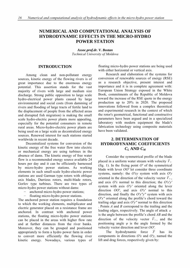
thin shell thbetween laDiscretizaticover and Sfig. 17. Thdeformationthe degrees 17) ux=0, uyon line C, u

Figure 17

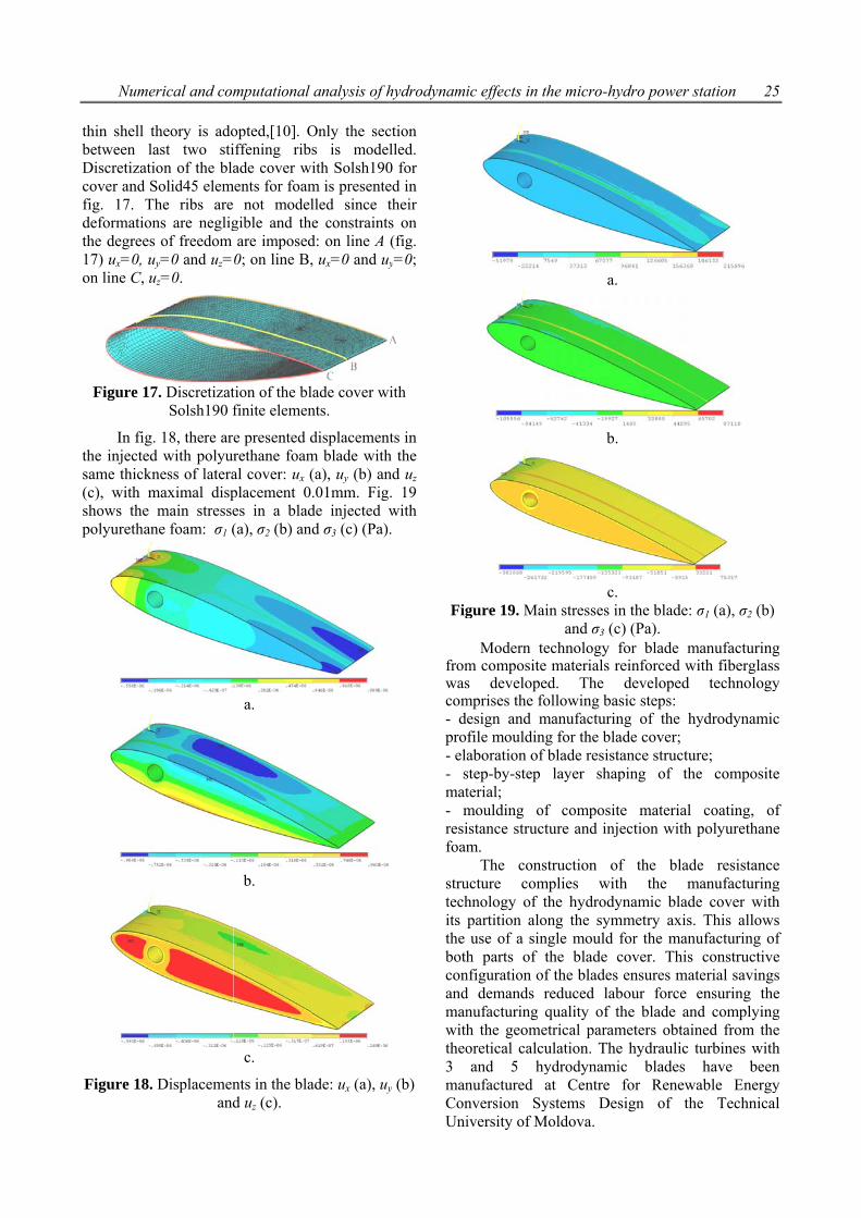
In fig.the injectedsame thickn(c), with mshows the polyurethan

Figure 18.

rical and com

heory is adoast two stion of the bla

Solid45 elemhe ribs are ns are neglig

of freedom y=0 and uz=

uz=0.

7. DiscretizatSolsh190 f

18, there ard with polyurness of lateramaximal disp

main stressene foam: σ1 (

Displacemenand

mputational

opted,[10]. Oiffening ribade cover w

ments for foamnot model

gible and thare imposed0; on line B,

tion of the blfinite elemen

e presented drethane foamal cover: ux (placement 0es in a blad(a), σ2 (b) an

a.

b.

c.

nts in the blad uz (c).

analysis of h

Only the secs is mode

with Solsh190m is presentelled since te constraints

d: on line A, ux=0 and uy

lade cover wnts.

displacemenm blade with(a), uy (b) an.01mm. Figde injected wnd σ3 (c) (Pa)

ade: ux (a), uy

hydrodynami

ction lled. 0 for ed in their s on (fig. y=0;

ith

nts in h the nd uz . 19 with .

y (b)

Fig

fromwascom- dpro- ela- smat- mresifoam

strutechits the bothconandmanwiththeo3 manConUni

ic effects in t

gure 19. Ma

Modern tem composites developemprises the foesign and mfile mouldinaboration of step-by-step terial; moulding ofistance structm.

The consucture comhnology of tpartition alouse of a sin

h parts of nfiguration ofd demands rnufacturing h the geomeoretical calcuand 5 hy

nufactured nversion Syiversity of M

the micro-hy

a.

b.

c. in stresses in

and σ3 (c)echnology fe materials reed. The ollowing basmanufacturing for the bla

f blade resistalayer shap

f compositeture and inje

struction ofmplies withthe hydrodynong the symngle mould fthe blade cf the blades reduced labquality of th

etrical paramulation. Theydrodynamicat Centre fystems Des

Moldova.

ydro power st

n the blade: σ) (Pa). for blade maeinforced wideveloped

sic steps: ng of the hyde cover; ance structurping of the

e material ection with p

f the bladeh the manamic blade

mmetry axis. for the manucover. This ensures mate

bour force ehe blade and

meters obtain hydraulic tuc blades for Renewa

sign of the

tation 25

σ1 (a), σ2 (b)

anufacturingth fiberglass

technology

ydrodynamic

re; e composite

coating, ofpolyurethane

e resistanceanufacturinge cover withThis allows

ufacturing ofconstructiveerial savingsensuring thed complyingned from theurbines withhave been

able Energye Technical

5

g s y

c

e

f e

e g h s f e s e g e h n y l

26 Num

7HY

Based

elaborated turbines witof the bladdirection. Tconfiguratiostations for electric or m

Fig. 2micro hydroblades usedpresented hydropowerMHCF D4with 5 blabearings in 3 with electit is placedblades guid

Figurhydr

3−mechan

Fig. 2station MHkinetic enerindustrial efig. 23 prinstalled on

erical and co

. FLOATAYDROPOW

d on carried otwo typo

th 3 and 5 bldes with reThere were pons of flo

conversion mechanic ene20 presents topower stati

d for water pthe constru

r station forx1,5E based

ades. The brotor 2 coup

tric generatod the spatiaing and orien

re 20. Kinemropower statinical gear, 4

21 and 22 shCF D4x1,5Ergy into elecnterprises fr

resents the n river Prut.

omputationa

ABLE MIWER STA

out research, -dimensions lades and optespect to thproposed [2

oatable micof river kin

ergy. he kinematicion MHCF Dpumping. In uctive concr electric end on the hy

blades 1 arepled through r 4. On the f

al truss 7 contation mech

matic scheme ion: 1−blade,5− bearings

how the mi

E for the conctric energy rom Republimicro hydr

al analysis of

CRO TIONS

there have bof hydra

timal orientahe water str], four differo hydropo

netic energy

c scheme ofD4x1,5M wi

fig. 21, thercept of m

nergy generaydraulic ture mounted wa planetary

floating bodioupled with hanism 6.

of a micro , 2−rotor,

s, 6−belt driv

icro hydroponversion of rmanufacture

ic Moldova, ropower sta

f hydrodynam

been aulic ation ream erent ower into

f the ith 5 re is

micro ation rbine with gear ies 5

the

ve.

ower river ed at

and ation

mic effects in

Figure 21. M

Figure 22. M

Figure 23. MD4x1

n the micro-hy

Micro hydropD4x1,5

Micro hydropD4x1,5

Micro hydrop,5E installed

hydro power s

power station5E.

power station5E.

power stationd on river Pru

station

n MHCF

n MHCF

n MHCF ut.


8. CONCLUSIONS

The hydraulic turbine with 5 hydrodynamic profile blades assures conversion of 49.5% of the energetic potential of water stream with velocity 1.3 m/s. The optimal orientation of the blades with respect to water stream direction (enabled by a guidance mechanism) assures participation of all blades (even those moving upstream) in generating the torque at the rotor shaft. The blades with composite materials cover injected with polyurethane foam and resistance structure with 5 stiffening ribs assure minimal local deformations that will not influence significantly the water flow and efficiency of energy conversion. Experimental testing of the micro hydropower station MHCF D4x1,5E in real field conditions confirmed that the hydropower station with hydrodynamic 5−blade rotor assures the conversion of the energy at the rotor shaft to the generator clams with efficiency of 77.5%.

References:

1. I. Bostan, V. Dulgheru, V. Bostan, R. Ciuperca. Anthology of Inventions: Systems for Renewable Energy Conversion. Ch.: “BonsOffices”SRL, 2009. 458pp. ISBN: 978-9975-80-283-3. 2. I. Bostan, V. Bostan, V. Dulgheru. Numerical modelling and simulation of the fluid flow action on rotor blades of the micro-hydropower station, Ovidius University Annals of Mechanical Engineering, Vol. VIII, Tom I, 2006, p.70-78. 3. J. Moran. An Introduction to Theoretical and Computational Aerodynamics, John Wiley and sons, 1984. 4. J. Katz, A. Plotkin. Low Speed Aerodynamics, From Wing Theory to Panel Methods, Mac-Graw Hill, 1991. 5. G.K. Batcelor. An Introduction to Fluid Dynamics, Cambridge University Press, 1970. 6. T. Cebeci, P. Bradshaw. Momentum Transfer in Boundary layers, Hemisphere Publishing Corportation, 1977. 7. W.C. Reynolds, T. Cebeci. Calculation of Turbulent Flows, Springer-Verlag, Topics in Applied Physics Series, Vol.12, 1978. 8. R.Michel. Etude de la Transition sur les Profiles d’Ales, Onera Report, 1/1578A, 1951. 9. H.B. Squire, A.D. Young. The Calculation of the Profile Drag of Aerofoils, R.&M.1838, ARC Technical Report , London, 1938.

10. P. G. Ciarlet. Mathematical Elasticity, vol.II. Theory of Plates, Elsevier Science B.V., Amsterdam, 1997. 11. R. M. Jones. Mechanics of Composite Materials, 2nd Edition, Taylor & Francis, 1999. 12. MIL-HDBK-17 Composite Materials Handbook. 13. ANSYS 10.0, User’s Guide. 14. ANSYS 10.0, Advanced Analysis Techniques Guide

Recommended for publication 12.03.2012.

numerical and computational analysis of hydrodynamic ... · numerical and computational analysis of...

Documents