numerical analysis course contents solution of non linear...
TRANSCRIPT

Numerical Analysis –MTH603 VU
© Copyright Virtual University of Pakistan 1
Numerical Analysis
Course Contents
Solution of Non Linear Equations
Solution of Linear System of Equations
Approximation of Eigen Values Interpolation and Polynomial Approximation
Numerical Differentiation
Numerical Integration
Numerical Solution of Ordinary Differential Equations
Introduction We begin this chapter with some of the basic concept of representation of numbers on
computers and errors introduced during computation. Problem solving using computers and the
steps involved are also discussed in brief.
Number (s) System (s)
In our daily life, we use numbers based on the decimal system. In this system, we use ten
symbols 0, 1,…,9 and the number 10 is called the base of the system.
Thus, when a base N is given, we need N different symbols 0, 1, 2, …,(N – 1) to represent an
arbitrary number.
The number systems commonly used in computers are
Base, N Number
2 Binary
8 Octal
10 Decimal
16 Hexadecimal
An arbitrary real number, a can be written as
1 1 1
1 1 0 1m m m
m mma a N a N a N a a N a N
! " " " " " " "
In binary system, it has the form,
1 1 1
1 1 0 12 2 2 2 2m m m
m m ma a a a a a a
! " " " " " " "
The decimal number 1729 is represented and calculated
3 2 1 0
10(1729) 1 10 7 10 2 10 9 10! # " # " # " #
While the decimal equivalent of binary number 10011001 is
0 1 2 3 4 5 6 7
10
1 2 0 2 0 2 1 2 1 2 0 2 0 2 1 2
1 1 11
8 16 128
(1.1953125)
# " # " # " # " # " # " # " #
! " " "
!
Electronic computers use binary system whose base is 2. The two symbols used in this system
are 0 and 1, which are called binary digits or simply bits.
The internal representation of any data within a computer is in binary form. However, we prefer
data input and output of numerical results in decimal system. Within the computer, the
arithmetic is carried out in binary form.
Conversion of decimal number 47 into its binary equivalent
Sol.

Numerical Analysis –MTH603 VU
© Copyright Virtual University of Pakistan 2
10 2(47) (101111)!
Binary equivalent of the decimal fraction 0.7625
Sol.
Product Integer
0.7625 x2 1.5250 1
0.5250 x2 1.0500 1
0.05 x2 0.1 0
0.1 x2 0.2 0
0.2 x2 0.4 0
0.4 x2 0.8 0
0.8 x2 1.6 1
0.6 x2 1.2 1
0.2 x2 0.4 0
10 2(0.7625) (0.11....11(0011))!
Conversion (59)10
into binary and then into octal.
Sol.
2 47 Remainder
2 23 1
2 11 1
2 5 1
2 2 1
2 1 0
0 1 Most significant
bit
229 1
214 1
27 0
23 1
21 1
0
1

Numerical Analysis –MTH603 VU
© Copyright Virtual University of Pakistan 3
10 2(59) (11011)!
2 8(111011) 111011 (73)! !

Numerical Analysis –MTH603 VU
© Copyright Virtual University of Pakistan 1
Errors in Computations Numerically, computed solutions are subject to certain errors. It may be fruitful to
identify the error sources and their growth while classifying the errors in numerical
computation. These are
Inherent errors,
Local round-off errors
Local truncation errors
Inherent errors
It is that quantity of error which is present in the statement of the problem itself, before
finding its solution. It arises due to the simplified assumptions made in the mathematical
modeling of a problem. It can also arise when the data is obtained from certain physical
measurements of the parameters of the problem.
Local round-off errors
Every computer has a finite word length and therefore it is possible to store only a fixed
number of digits of a given input number. Since computers store information in binary
form, storing an exact decimal number in its binary form into the computer memory gives
an error. This error is computer dependent.
At the end of computation of a particular problem, the final results in the computer,
which is obviously in binary form, should be converted into decimal form-a form
understandable to the user-before their print out. Therefore, an additional error is
committed at this stage too.
This error is called local round-off error.
10 2(0.7625) (0.110000110011)
If a particular computer system has a word length of 12 bits only, then the decimal
number 0.7625 is stored in the computer memory in binary form as 0.110000110011.
However, it is equivalent to 0.76245.
Thus, in storing the number 0.7625, we have committed an error equal to 0.00005, which
is the round-off error; inherent with the computer system considered.
Thus, we define the error as
Error = True value – Computed value
Absolute error, denoted by |Error|,
While, the relative error is defined as
Relative error Error
True value
Local truncation error
It is generally easier to expand a function into a power series using Taylor series
expansion and evaluate it by retaining the first few terms. For example, we may
approximate the function f (x) = cos x by the series
2 4 2
cos 1 ( 1)2! 4! (2 )!
nnx x x
xn
! " ! " ! "
If we use only the first three terms to compute cos x for a given x, we get an approximate
answer. Here, the error is due to truncating the series. Suppose, we retain the first n
terms, the truncation error (TE) is given by

Numerical Analysis –MTH603 VU
© Copyright Virtual University of Pakistan 2
2 2
TE(2 2)!
nx
n
"
#"
The TE is independent of the computer used.
If we wish to compute cos x for accurate with five significant digits, the question is, how
many terms in the expansion are to be included? In this situation
2 2
5 6.5 10 5 10(2 2)!
nx
n
"
! !$ % %
"
Taking logarithm on both sides, we get
10 10
(2 2) log log[(2 2)!]
log 5 6log 10 0.699 6 5.3
n x n" ! "
$ ! ! !
or
log[(2 2)!] (2 2) log 5.3n n x" ! " &
We can observe that, the above inequality is satisfied for n = 7. Hence, seven terms in the
expansion are required to get the value of cos x, with the prescribed accuracy
The truncation error is given by
16
TE16!
x#

Numerical Analysis –MTH603 VU
© Copyright Virtual University of Pakistan 1
Polynomial
An expression of the form 1 2
0 1 2 1( ) ...n n n
n nf x a x a x a x a x a
! " " " " " where n is a
positive integer and 0 1 2, , .... na a a a" are real constants, such type of expression is called
an nth degree polynomial in x if 0 0a #
Algebraic equation:
An equation f(x)=0 is said to be the algebraic equation in x if it is purely a polynomial in
x.
For example
5 4 23 6 0x x x x" " " ! It is a fifth order polynomial and so this equation is an algebraic
equation. 3
6
4 3 2
4 2
6 0
0
4 3 2 0
6 21 0
x
x x
y y y y polynomial in y
t t polynomail in t
! $
$ % ! $
" ! $ $ $
! $ $ $
These all are the examples of the polynomial or algebraic equations.
Some facts
1. Every equation of the form f(x)=0 has at least one root ,it may be real or complex.
2. Every polynomial of nth degree has n and only n roots.
3. If f(x) =0 is an equation of odd degree, then it has at least one real root whose sign is
opposite to that of last term.
4.If f(x)=0 is an equation of even degree whose last term is negative then it has at least
one positive and at least one negative root .
Transcendental equation
An equation is said to be transcendental equation if it has logarithmic, trigonometric and
exponential function or combination of all these three.
For example
5 3 0xe x ! it is a transcendental equation as it has an exponential function
2
sin 0
ln sin 0
2sec tan 0
x
x
e x
x x
x x e
!
!
!
These all are the examples of transcendental equation.
Root of an equation
For an equation f(x) =0 to find the solution we find such value which satisfy the equation
f(x)=0,these values are known as the roots of the equation .
A value a is known as the root of an equation f(x) =0 if and only if f (a) =0.

Numerical Analysis –MTH603 VU
© Copyright Virtual University of Pakistan 2
Properties of an Algebraic equation
1. Complex roots occur in the pairs. That is ,If (a+ib ) is a root of f(x)=0 then (a-ib )
is also a root of the equation
2. if x=a is a root of the equation f(x)=0 a polynomial of nth degree ,then (x-a) is a
factor of f(x) and by dividing f(x) by (x-a) we get a polynomial of degree n-1.
Descartes rule of signs
This rule shows the relation ship between the signs of coefficients of an equation and
its roots.
“The number of positive roots of an algebraic equation f(x) =0 with real coefficients
can not exceed the number of changes in the signs of the coefficients in the polynomial
f(x) =0.similarly the number of negative roots of the equation can not exceed the number
of changes in the sign of coefficients of f (-x) =0”
Consider the equation 3 23 4 5 0x x x " ! here it is an equation of degree three and
there are three changes in the signs
First +ve to –ve second –ve to +ve and third +ve to –ve so the tree roots will be positive
Now 3 2( ) 3 4 5f x x x x ! so there is no change of sign so there will be no negative
root of this equation.
Intermediate value property
If f(x) is a real valued continuous function in the closed interval a x b& & if f(a) and f(b)
have opposite signs once; that is f(x)=0 has at least one root ' $ such that a b'& &
Simply
If f(x)=0 is a polynomial equation and if f(a) and f(b) are of different signs ,then f(x)=0
must have at least one real root between a and b.
Numerical methods for solving either algebraic or transcendental equation are classified
into two groups
Direct methods
Those methods which do not require any information about the initial approximation of
root to start the solution are known as direct methods.
The examples of direct methods are Graefee root squaring method, Gauss elimination
method and Gauss Jordan method. All these methods do not require any type of initial
approximation.
Iterative methods
These methods require an initial approximation to start.

Numerical Analysis –MTH603 VU
© Copyright Virtual University of Pakistan 3
Bisection method, Newton raphson method, secant method, jacobie method are all
examples of iterative methods.
How to get an initial approximation?
The initial approximation may be found by two methods either by graphical method or
analytical method
Graphical method
The equation f(x)=0 can be rewritten as 1 2( ) ( )f x f x$! and initial approximation of f(x)
may be taken as the abscissa of the point of intersection of graphs of
1 2( ) ( )y f x and y f x! $ $ ! $
for example ( ) sin 1 0f x x x! !
so this may be written as 1 sinx x ! Now we shall draw the graphs of
1 siny x and y x! $ $ !
Here both the graphs cut each other at 1.9 so the initial approximation should be taken as
1.9
Analytical method
This method is based on the intermediate value property in this we locate two values a
and b such that f(a) and f(b) have opposite signs then we use the fact that the root lies

Numerical Analysis –MTH603 VU
© Copyright Virtual University of Pakistan 4
between both these points ,this method can be used for both transcendental and algebraic
equations.
Consider the equation
(0) 1
180(1) 3 1 sin(1 ) 3 1 0.84147 1.64299
f
f(
!
! " ) ! " !
Here f(0) and f(1) are of opposite signs making use of intermediate value property we
infer that one root lies between 0 and 1 .
So in analytical method we must always start with an initial interval (a,b) so that f(a) and
f(b) have opposite signs.
Bisection method (Bolzano)
Suppose you have to locate the root of the equation f(x)=0 in an interval say 0 1( , )x x ,let
0( )f x and 1( )f x are of opposite signs such that 0 1( ) ( ) 0f x f x *
Then the graph of the function crossed the x-axis between 0 1x and x$ $ which exists the
existence of at least one root in the interval 0 1( , )x x .
The desired root is approximately defined by the mid point 0 12
2
x xx
"! if 2( ) 0f x ! then
2x is the root of the equation otherwise the root lies either between 0 2x and x$ or 1 2x and x$
Now we define the next approximation by 0 23
2
x xx
"! provided 0 2( ) ( ) 0f x f x * then
root may be found between 0 2x and x$
If provided 1 2( ) ( ) 0f x f x * then root may be found between 1 2x and x$ by 1 23
2
x xx
"!
Thus at each step we find the desired root to the required accuracy or narrow the range to
half the previous interval.
This process of halving the intervals is continued in order to get smaller and smaller
interval within which the desired root lies. Continuation of this process eventually gives
us the required root.
NOTE: In numerical analysis all the calculation are carried out in radians mode
and the value of pi is supposed to be 3.14
Example
Solve 3 9 1 0x x " ! for the root between x=2 and x=4 by bisection method
Solution:
Here we are given the interval (2,4) so we need not to carry out intermediate value
property to locate initial approximation.
Here
( ) 3 1 sin 0f x x x! " !

Numerical Analysis –MTH603 VU
© Copyright Virtual University of Pakistan 5
3
3
3
( ) 9 1 0
(2) 2 9(2) 1 8 18 1 9
(4) 4 9(4) 1 64 36 1 29
(2) (3) 0 2 4
f x x x
now f
f
here f f so root lies between and
! " !
$ ! " ! " !
$$$$$$$ ! " ! " !
$ $$ * $ $ $ $ $ $ $ $
0 1
2
3
3
3
2 43
2
(3) 3 9(3) 1 27 27 1 1
(2) (3) 0 2 3
2 32.5
2
(2.5) 2.5 9(2.5) 1 15.625 22.5 1 5.875 0
2.5 3 (2.5) (3)
x x
x
f
here f f so the root lies between nad
x
f
so the root lies between and as f f
! +$$$$ ! ,$$$
"! !
! " ! " !
$ * $ $ $ $ $ $ $ $ $
"! !
! " ! " ! *
$ $ $ $ $ $ $ $ $ *
4
5 6
0
2.5 32.75
2
2.875 2.9375
.
x
now
similarly x and x and the process is continued
untill the desired accuracy is obtained
"! !
$
$ ! $ $ ! $ $ $ $ $ $
$ $ $ $ $
n xn f ( xn )
2 3 1.0
3 2.5 -5.875
4 2.75 -2.9531
5 2.875 -1.1113
6 2.9375 -0.0901
When to stop the process of iteration?
Here in the solved example neither accuracy is mentioned and nor number of iteration is
mentioned by when you are provided with the number of iteration then you will carry
those number of iteration and will stop but second case is accuracy like you are asked to

Numerical Analysis –MTH603 VU
© Copyright Virtual University of Pakistan 6
find root with an accuracy of 310 then you will check the accuracy by subtracting two
consecutive root like 2.135648 and 2.135769
2.135769-2.135648=0.000121
So the accuracy of 310 is achieved so you will stop here.
Example:
Carry out the five iterations for the function 2( ) 2 cos(2 ) ( 1)f x x x x! "
Note: All the calculations should be done in the radians.
Solution: 2
2
2
2
2
( ) 2 cos(2 ) ( 1)
( 1) 2( 1)cos( 2) ( 1 1) 2( 0.4161) 0.8322 0
(0) 2(0)cos(0) (0 1) 1 1 0
0 1 (0) ( 1) 0
0 10.5
2
( 0.5) 2( 0.5)cos( 1) ( 0.5 1) 0.5403
f x x x x
f
f
so the root lies between and as f f
x
f
! "
! " ! ! " -
! " ! ! *
$ $ $ $ $ $ $ $ $ *
! !
! " !
3
2
4
0.25 0.7903 0
1 0.5 ( 1) ( 0.5)
0.5 10.75
2
( 0.75) 2( 0.75)cos( 1.5) ( 0.75 1) 0.106 0.0625 0.1686 0
1 0.75 ( 1) ( 0.75)
0.75 1
2
so root lies between and as f f
x
f
so root lies between and as f f
x
! *
$ $ $ $ $ $ $ $
! !
! " ! ! *
$ $ $ $ $ $ $ $
!
2
5
0.875
( 0.875) 2( 0.875)cos( 1.75) ( 0.875 1) 0.3119 0.015625 0.296275 0
0.875 0.75 ( 0.75) ( 0.875)
0.75 0.8750.8125
2
( 0.8125) 2( 0.8125)cos( 1.625) ( 0.8125 1)
f
so root lies between and as f f
x
f
!
! " ! ! -
$ $ $ $ $ $ $ $
! !
! " 2
5
0.0880 0.0351 0.052970 0
0.8125 0.75 ( 0.75) ( 0.8125)
0.75 0.81250.78125
2
so root lies between and as f f
x
! ! -
$ $ $ $ $ $ $ $
! !
Example :
Carry out the first five iterations 2( ) cos 2 3 1 1.2 1.3f x x x x x x! " $$$.$$$ & &
Note: All the calculations should be done in the radians.
Solution:

Numerical Analysis –MTH603 VU
© Copyright Virtual University of Pakistan 7
2
2
2
( ) cos 2 3 1
(1.2) 1.2cos1.2 2(1.2) 3(1.2) 1
1.2(0.3623) 2(1.44) 3.6 1
(1.3) 1.3cos1.3 2(1.3) 3(1.3) 1
1.3(0.2674) 2(1.69) 9.3 1
(1.2) (1.3) 0
f x x x x x
f
f
as f f
! " $
! " $
$$$$$$$$$$$! " $! /012,3 - /
! " $
$$$$$$$$$$$! " $! /014++ * /
$ *
2
2
3
1.2 1.31.25
2
(1.25) 1.25cos1.25 2(1.25) 3(1.25) 1
1.25(0.3153) 2(1.5625) 3.75 1
(1.25) (1.3) 0
1.25 1.31
2
so the root lies between both
x
f
as f f so the root lies between both
x
$ $ $ $ $ $ $
"! !
! " $
$$$$$$$$$$$! " $! /0/151- /
$ * $ $ $ $ $ $ $
"! !
2
4
.275
(1.275) 1.275cos1.275 2(1.275) 3(1.275) 1
1.275(0.2915) 2(1.6256) 3.825 1
(1.25) (1.275) 0
1.25 1.2751.2625
2
(1.2625) 1.2625cos1.2625
f
as f f so the root lies between both
x
f
! " $
$$$$$$$$$$$! " $! /0/2,2 * /
$ * $ $ $ $ $ $ $
"! !
! 2
5
2
2(1.2625) 3(1.2625) 1
1.275(0.3034) 2(1.5939) 3.7875 1
(1.25) (1.265) 0
1.25 1.26251.25625
2
(1.25625) 1.25625cos1.25625 2(1.25625) 3(1.256
as f f so the root lies between both
x
f
" $
$$$$$$$$$$$! " $! /0/1%+ * /
$ * $ $ $ $ $ $ $
"! !
! "
6
25) 1
1.25625(0.3093) 2(1.5781) 3(1.25625) 1 0.00108
(1.25625) (1.265) 0
1.25625 1.26251.259375
2
as f f so the root lies between both
x
$
$$$$$$$$$$$! " ! $- /
$ * $ $ $ $ $ $ $
"! !

Numerical Analysis –MTH603 VU
© Copyright Virtual University of Pakistan 1
Regula-Falsi method (Method of false position)
Here we choose two points nx and 1nx such that 1( ) ( )n nf x and f x ! ! have opposite signs.
Intermediate value property suggests that the graph of the y=f(x) crosses the x-axis
between these two points and therefore, a root lies between these two points.
Thus to find the real root of f(x)=0 using Regula-Falsi method ,we replace the part of the
curve between the points 1 1( , ( )) ( , ( ))n n n nA x f x and B x f x !! ! by a chord in the interval and
we take the point of intersection of this chord with x-axis as initial approximation.
Now, the equation of the chord joining the points A and B is,
1 1
( )
( ) ( )
n n
n n n n
y f x x x
f x f x x x
"
Setting y=0 in the above equation we get
1
1
( )( ) ( )
n nn n
n n
x xx x f x
f x f x
"
Hence the first approximation to the root is given by
11
1
( )( ) ( )
n nn n n
n n
x xx x f x
f x f x
#
"
We observe that 1 1( ) ( )n nf x and f x #! ! are of opposite signs thus it is possible to apply the
above procedure, to determine the line through B and 1A and so on.
Hence for successive approximation to the root above formula is used.
Example
Use the Regula-Falsi method to compute a real root of the equation x3 – 9x + 1 = 0,
(i) if the root lies between 2 and 4
(ii) if the root lies between 2 and 3.
Comment on the results.
Solution
Let
3 3
f (x) = x3 - 9x + 1
f (2) = 2 - 9(2) + 1=8 18+1= 9and f (4) = 4 - 9(4) + 1=64 36+1=29. ! ! !! !! !
Since f (2) and f (4) are of opposite signs, the root of f (x) = 0 lies between 2 and 4.
Taking x1 = 2, x2 = 4 and using Regula-Falsi method, the first approximation is given by
2 13 2 2
2 1
4 2 2(29)( ) 4 (29) 4
( ) ( ) 29 ( 9) 38
584 4 1.5263 2.4736
38
x xx x f x
f x f x
" " "
!!!!" " "

Numerical Analysis –MTH603 VU
© Copyright Virtual University of Pakistan 2
Now 3f (x3) = 2.4736 - 9(2.4736) + 1=15.13520-22.2624+1= -6.12644.
Since f (x2) and f (x3) are of opposite signs, the root lies between x2 and x3.
The second approximation to the root is given as
Therefore 3f (x4) = 2.73989 - 9(2.73989) + 1=20.5683-24.65901+1= =- 3. 090707.
Now, since f (x2) and f (x4) are of opposite signs, the third approximation is obtained
from
Now 3f (x5) = 2.86125 - 9(2.86125) + 1=23.42434-25.75125+1= -1.326868.
(ii)
Here
3 3
f (x) = x3 - 9x + 1
f (2) = 2 - 9(2) + 1 = 8 18 +1=- 9 and f (3) = 3 - 9(3) + 1= 27 27+1= 1. !! ! ! ! !
Since f (2) and f (3) are of opposite signs, the root of f (x) = 0 lies between 2 and 3.
Taking x1 = 2, x2 = 3 and using Regula-Falsi method, the first approximation is given by
Since f (x2) and f (x3) are of opposite signs, the root lies between x2 and x3.
The second approximation to the root is given as
4
4
3
4
2.9 3 0.1 0.12.9 ( 0.711) 2.9 ( 0.711) 2.9 ( 0.711)
0.711 1 1.711 1.711
2.9 (0.05844)( 0.711) 2.9 _ 0.04156 2.94156
( ) 0.0207
f (x ) = 2.94156 - 9(2.94156) + 1 =25.45265 26.47404+1= 0.0207
x
f x
" " "
!!!!" " "
"
! ! ! !
3 24 3 3
3 2
2.4736 4( ) 2.4736 ( 6.12644)
( ) ( ) 6.12644 29
1.52642.4736 ( 6.12644) 2.4736 (0.04345)( 6.12644)
35.12644
2.4736 0.26619 2.73989
x xx x f x
f x f x
" "
!!!!" "
!!!!" # "
4 25 4 4
4 2
2.73989 4( ) ( 3.090707) 2.86125
( ) ( ) 3.090707 29
1.26011( 3.090707) 0.039267(3.090707) 2.86125
32.090707
x xx x f x
f x f x
" "!$%&'()( "!!
!!!!"!$%&'()( "!$%&'()( # " $%&'()(# *%+$+',' "!
2 13 2 2
2 1
3
3
3 2( ) 3 (1)
( ) ( ) 1 9
13 2.9
10
f (x ) = 2.9 - 9(2.9) + 1 =24.389 26.1+1= 0.711
x xx x f x
f x f x
" "
#
!!!!" "
! ! ! !

Numerical Analysis –MTH603 VU
© Copyright Virtual University of Pakistan 3
Now, we observe that f (x2) and f (x4) are of opposite signs; the third approximation is
obtained from
5
3
5
2.94156 3 0.058442.94156 ( 0.0207) 2.94156 ( 0.0207)
0.0207 1 1.0207
2.94156 ( 0.05725)( 0.0207) 2.94275
f (x ) = 2.94275 - 9(2.94275) + 1 =25.48356 = 0.0011896
x
" "
" "
! !$,%-)-&.#+
We observe that the value of the root as a third approximation is evidently different in
both the cases, while the value of x5, when the interval considered is (2, 3), is
closer to the root.
Important observation: The initial interval (x1, x2) in which the root of the equation
lies should be sufficiently small.
Example
Use Regula-Falsi method to find a real root of the equation lnx – cos x = 0
accurate to four decimal places after three successive approximations.
Note: here is a transcendental equation all the calculation should be done in the
radians mode
Sol:
3
( ) ln x - cos x
we have
f(1)=ln1-cos(1)=0-0.540302=-0.540302<0
f(2)=ln2-cos(2)=0.69315-0.41615=1.109
As f(1)f(2)<0 so the root lies between1and 2
the first approximation is
2 12
1.1
f x
obtained form
x
"
! !
! ! ! ! ! ! ! ! ! !
! ! ! ! ! !
"
3
(1.109)09 0.540302
1.10932 1.3275
1.6496
( ) ln 1.3275 - cos 1.3275 02833 0.2409 0.0424f x
#
" "
" " "
Now, since f (x1) and f (x3) are of opposite signs, the second approximation is obtained as
4
3
4
(.3275)(.0424)1.3275
0.0424 0.5403
1.3037
( ) ln 1.3037 - cos 1.3037 =1.24816 10
x
f x
" #
"
" /

Numerical Analysis –MTH603 VU
© Copyright Virtual University of Pakistan 4
Similarly, we observe that f (x1) and f (x4) are of opposite signs, so, the third
approximation is given by
5
4
5
(0.3037)(0.001248)1.3037
0.001248 0.5403
1.3030
( ) 0.6245 10
x
f x
" #
"
" /
The required real root is 1.3030
Example:
Use method of false position to solve 2 2cos 6 0 1 2x xe x x # # " !!!!!! 0 0
Solution:
0 1
11
1
1 1
2 2
1 02 1
1
( ) 2 2cos
1 , 2
( )( ) ( )
(1) 2 2cos1 6
(2) 2 2cos 2 6
1
( )
x x
n nn n
n n
f x e x
x x
now
x xx f x
f x f x
f e
f e
now for n
x xx x
f x
#
" # # ! ,
" !!! !!!! "
!
"
" # # !" $%&+)$# *%.# $1*%.-*'2 , " +%&*++
" # # !" &%')),# *%$.# $1 *%-+,+2 , " *%)*,)
! ! "
" 1
0
2
1.6783 1.6783
2 13 2 2
2 1
3
2 1( ) 2 (0.8068)
( ) 0.8068 1.7011
12 (0.8068) 1.6783
2.5079
(1.6783) 2 2cos(1.6783) 6
2
1.6783 2( ) 1.6783 ( 0.5457)
( ) ( ) ( 0.5457) 0.8068
1.6
f xf x
x
f e
now for n
x xx x f x
f x f x
x
"
#
" "
" # # !" *%.-.&
! ! "
" "
"( 0.3217)
783 ( 0.5457) 1.6783 0.12979 1.8081( 1.3525)
" # "

Numerical Analysis –MTH603 VU
© Copyright Virtual University of Pakistan 5
1.6783 1.8081
3 24 3 3
3 2
3
(1.8081) 2 2cos(1.8081) 6
3
1.8081 1.6783( ) 1.8081 ( 0.08575)
( ) ( ) ( 0.08575) 0.5457
0.12981.8081 ( 0.08575) 1.6783 0.12979 1.8323
0.45995
(1.8323)
f e
now for n
x xx x f x
f x f x
x
f
" # # !" *%).&.
! ! "
" "
#
" " # "
1.8323 1.8323
4 35 4 4
4 3
5
1.8293 1.8
2 2cos(1.8323) 6
4
1.8323 1.8081( ) 1.8323 (0.01199)
( ) ( ) 0.01199 0.08575
0.02421.8323 (0.01199) 1.8323 0.00296 1.8293
0.09774
(1.8293) 2
e
now for n
x xx x f x
f x f x
x
f e
" # # !" *%++((
! ! "
" "
#
" " "
" # 293
5 46 5 5
5 4
6
2cos(1.8293) 6
5
1.8293 1.8323( ) 1.8293 ( 0.000343)
( ) ( ) 0.000343 0.01199
( 0.003)1.8293 ( 0.000343) 1.8293
0.012333
now for n
x xx x f x
f x f x
x
# !" *%***'-'
! ! "
" "
" "
Example:
Solve the equation 22 cos 2 ( 2) 0 2 3x x x x " !!! 0 0 Perform only three iterations.
Solution
2
0 1
2
2
11
1
1 02 1 1
1 0
( ) 2 cos 2 ( 2)
2 3
(2) 2(2)cos 4 (2 2) 4cos 4 2.6146
(3) 2(3)cos 2(3) (3 2) 6cos 6 1 4.7610
( )( ) ( )
1
3 2( ) 3
( ) ( ) 4.7610 2.
n nn n n
n n
f x x x x
here x and x
so f
f
x xhere x x f x
f x f x
for n
x xx x f x
f x f x
#
"
! " ! ! " !
! " " "
" " "
! "
! "
" "
(4.7610)
4146

Numerical Analysis –MTH603 VU
© Copyright Virtual University of Pakistan 6
2
2 13 2 2
2 1
13 (4.7610) 3 0.6455 2.3545
7.3756
(2.3545) 2(2.3545)cos 2(2.3545) (2.3545 2) 4.709cos 4.709 0.1257 0.1416
2
2.3545 3( ) 2.3545 ( 0.1416)
( ) ( ) 0.1416 4.7610
2.3731
(2.3713)
f
for n
x xx x f x
f x f x
f
" " "
" " "
! " !
" "
!!!!"
2
3 24 3 3
3 2
2
2(2.3713)cos 2(2.3713) (2.3713 2) 4.7462cos 4.7462 0.1392 0.1392
3
2.3731 2.3545( ) 2.3713 (0.0212)
( ) ( ) 0.0212 0.1416
2.3707
(2.3707) 2(2.3707)cos 2(2.3707) (2.3707 2) 4.7
for n
x xx x f x
f x f x
f
" " "
! " !
" "
#
!!!!"
" "
4 35 4 4
4 3
414cos 4.7412 0.1374 0.00013
4
2.3707 2.3731( ) 2.3707 (0.00013)
( ) ( ) 0.00013 0.0212
2.3707
for n
x xx x f x
f x f x
"
! " !
" "
!!!!"

Numerical Analysis –MTH603 VU
© Copyright Virtual University of Pakistan 1
Example
Using Regula-Falsi method, find the real root of the following equation correct, to three
decimal places: x log 10 x =1.2
Solution:
10
10
10
Let f (x) = x log x 1.2
f (2) = log 2 1.2 = 0.5979,
f (3) = 3 log 3 1.2 = 0.2314.
Since f (2) and f (3) are of opposite signs, the real root lies betweenx1 = 2, x2 = 3.
!
" ! !
!
The first approximation is obtained from
2 13 2 2
2 1
3 10
3 2( ) 3 (0.2314)
( ) ( ) 0.2314 0.5979
0.23143 2.72097
0.8293
( ) Let f (x) = 2.72097log 2.72097 1.2 = 0.01713.
x xx x f x
f x f x
f x
! !# ! # !
! $
# ! #
# ! !
Since f (x2) and f (x3) are of opposite signs, the root of f (x) = 0 lies between x2 and
x3. Now, the second approximation is given by
3 24 3 3
3 2
4
4 10
2.72097 3( ) 2.72097 ( 0.1713) 2.7402
( ) ( ) 0.1713 0.2314
( ) = 2.7402 log 2.7402 1.2 3.8905 10
x xx x f x
f x f x
f x !
! !# ! # ! ! #
! ! !
! ! %
Thus, the root of the given equation correct to three decimal places is 2.740
NOTE: Here if TOL is given then we can simply find the value of TOL by subtracting
both the consecutive roots and write it in the exponential notation if the required TOL is
obtained then we stop.
Method of Iteration
Method of iterations can be applied to find a real root of the equation f (x) = 0 by
rewriting the same in the form.
( )x x&#
Let 0x x# be the initial approximation to the actual root, say, ' of the equation .then the
first approximation is 1 0( )x x&# and the successive approximation are 2 1( )x x&#
3 2 4 3 1( ), ( ),..., ( )n nx x x x x x& & & !# # # if sequence of the approximate roots, 1 2 3, , ,... nx x x x
converges to ' it is taken as the root of the equation f(x)=0.
For convergence purpose the initial approximation is to be done carefully.the choice
of the 0x is done according to the theorem.

Numerical Analysis –MTH603 VU
© Copyright Virtual University of Pakistan 2
Theorem
If ' be a root of f(x) =0 which is equivalent to ( )x x&# I be any interval containing the
point x=' and | '( ) | 1 ,x x I then the sequence of approximations& () * 1 2 3, , ,... nx x x x will
converge to the root ' provided that the initial approximation 0x is chosen in I
Example,
f (x) = cos x - 2x + 3 = 0.
It can be
Rewritten as 1
(cos 3) ( )2
x x x&# $ #
1( ) (cos 3)
2
f (x) = cos x - 2x + 3 = 0.
f(1)=cos 1 - 2(1) + 3 =1.54030>0
f(2)=cos 1 - 2(2) + 3 =-0.041614-4+3=-1.41614<0
so root lies between1and 2
1'( ) (sin )
2
'(1) '(2) 1
x x
x x
both and so the method
&
&
& &
# $
# !
)
0
1 0
2 1
3 2
1.5
1 1(cos 3) (cos(1.5) 3) 1.999825
2 2
1 1(cos 3) (cos(1.999825) 3) 1.999695
2 2
1 1(cos 3) (cos(1.999625) 3) 1.999695
2 2
of iterations can be applied
let x
x x
x x
x x
#
# $ # $ #
# $ # $ #
# $ # $ #
So this is the required root correct up to 5 places of decimal.
Example
Find the real root of the equation 3 2 1x x$ ! # + by method of iterations
Solution 3 2
3 2
3 2
( ) 1
(0) 0 0 1 1 0
(1) 1 1 1 1 0
0 1
let f x x x
now f
f
hence a real root lies between and
# $ !
# $ ! # ! )
# $ ! # ,

Numerical Analysis –MTH603 VU
© Copyright Virtual University of Pakistan 3
3 2
2
2
3
2
5
2
0
1 0
0
2 1
1
1 0
( 1) 1
1 1( )
( 1) 1
'( ) 1/ 2[1/( 1) ]
'(0) 1/ 2 1 '(1) 1/ 2 1
'( ) 1 int
0.65
1 1( ) 0.7784989
1 1.65
1( )
here
x x
x x
x x xx x
here x x
and
so x for all the values in the erval
let x
x xx
x xx
&
&
& &
&
&
&
$ ! #
$ #
# - # #$ $
# ! $
# ) # )
)
#
# # # #$
# #
3 2
2
4 3
3
5 4
4
6 5
5
7 6
6
8
10.7498479
1 1.7784989
1 1( ) 0.7559617
1 1.7498479
1 1( ) 0.7546446
1 1.7559617
1 1( ) 0.7549278
1 1.7546446
1 1( ) 0.7548668
1 1.7549278
1 1( ) 0.7548799
1 1.7548668
x xx
x xx
x xx
x xx
x xx
x
&
&
&
&
&
# #$
# # # #$
# # # #$
# # # #$
# # # #$
# # # #$
7
7
9 8
8
10 9
9
11 10
10
1 1( ) 0.7548771
1 1.7548799
1 1( ) 0.7548777
1 1.7548771
1 1( ) 0.7548776
1 1.7548777
1 1( ) 0.7548776
1 1.7548776
0.7548776
xx
x xx
x xx
x xx
hence root is
&
&
&
&
# # # #$
# # # #$
# # # #$
# # # #$
Note: In this question the accuracy up to 7 places is acquires or here the TOL is 710!

Numerical Analysis –MTH603 VU
© Copyright Virtual University of Pakistan 4
Example
Find a real root of the equation cos 3 1x x# ! correct to seven places of decimal.
Solution
Here it is a transcendental function and all the calculation must be done in the radians
mode and value of pi should be 3.14
( ) cos 3 1
(0) cos 0 3(0) 1 1 0
( / 2) cos(1.57) 3(1.57) 1 0.0007963 4.71 1 3.7092037 0
0 / 2
1( ) (cos 1)
3
1'( ) sin
3
1 si
f x x x
f
f
so a real root lies between and
here x x
we have x x
it is clearly less than as
.
.
&
&
# ! $
# ! $ # ,
# ! $ # ! $ # ! )
# $
# !
0
n ' 1 1
0.5
is a bounded function and it s values lies between and
hence iteration method can be applied
let x be the inital approximation then
!
#
1 0
2 1
3 2
4 3
5 4
6 5
1( ) [cos(0.5) 1] 0.6258608
3
1( ) [cos(0.6258608) 1] 0.6034863
3
1( ) [cos(0.6034863) 1] 0.6077873
3
1( ) [cos(0.6077873) 1] 0.6069711
3
1( ) [cos(0.6069711) 1] 0.6071264
3
1( )
3
x x
x x
x x
x x
x x
x x
&
&
&
&
&
&
# # $ #
# # $ #
# # $ #
# # $ #
# # $ #
# # [cos(0.6071264) 1] 0.6070969$ #

Numerical Analysis –MTH603 VU
© Copyright Virtual University of Pakistan 5
7 6
8 7
9 8
10 9
1( ) [cos(0.6070969) 1] 0.6071025
3
1( ) [cos(0.6071025) 1] 0.6071014
3
1( ) [cos(0.6071014) 1] 0.6071016
3
1( ) [cos(0.6071016) 1] 0.6071016
3
x x
x x
x x
x x
&
&
&
&
# # $ #
# # $ #
# # $ #
# # $ #

Numerical Analysis –MTH603 VU
© Copyright Virtual University of Pakistan 1
Newton -Raphson Method
This method is one of the most powerful method and well known methods, used for
finding a root of f(x)=0 the formula many be derived in many ways the simplest way to
derive this formula is by using the first two terms in Taylor’s series expansion of the
form,
1 1
1
1
1
( ) ( ) ( ) '( )
( ) 0 ,
( ) ( ) '( ) 0
, ,
( )0,1, 2...
'( )
n n n n n
n
n n n n
nn n
n
f x f x x x f x
setting f x gives
f x x x f x
thus on simplification we get
f xx x for n
f x
! "
# ! #
" !
# ## # #
! " # # !
Geometrical interpretation
Let the curve f(x)=0 meet the x-axis at x=$ meet the x axis at x=$ .it means that $ is
the original root of the f(x)=0.Let 0x be the point near the root $ of the equation f(x)=0
then the equation of the tangent 0 0 0[ , ( )]P x f x # is
0 0 0( ) '( )( )y f x f x x x" ! "
This cuts the x-axis at 01 0
0
( )
'( )
f xx x
f x! "
This is the first approximation to the root $ .if 1 1 1[ , ( )]P x f x # is the point corresponding
to 1x on the curve then the tangent at 1P # is
1 1 1( ) '( )( )y f x f x x x" ! "
This cuts the x-axis at 12 1
1
( )
'( )
f xx x
f x! "
This is the second approximation to the root $ .Repeating this process we will get the
root $ with better approximations quite rapidly.
Note:
1. When '( )f x # very large .i.e. is when the slope is large, then h will be small (as
assumed) and hence, the root can be calculated in even less time.
2. If we choose the initial approximation 0x close to the root then we get the root of
the equation very quickly.
3. The process will evidently fail if '( ) 0f x ! is in the neighborhood of the root. In
such cases the regula falsi method should be used.

Numerical Analysis –MTH603 VU
© Copyright Virtual University of Pakistan 2
4. If the initial approximation to the root is not given, choose two say, a and b, such
that f(a) and f(b) are of opposite signs. If |f(a)|<|f(b)| then take a as the initial
approximation.
5. Newton’s raphson method is also referred to as the method of tangents.
Example
Find a real root of the equation x3 – x – 1 = 0 using Newton - Raphson method, correct to
four decimal places.
Solution 3
3
3
2
2
2
f(x)=x - x - 1
f(1)=1 - 1 - 1 =-1<0
f(2)=2 - 2 - 1 = 8
1 2
'( ) 3 1 "( ) 6
'(1) 3*1 1
'( ) 3*2 1
"(1) 6
"(2) 6(2) 12
(
so the root lies between and
here f x x and f x x
f
f x
here
f
f
here f
# #" %#"&! ' ( )
# # # # # # # #
# ! " ###### ##### !
! " #! %
! " #!&&
#
!
! !
# 02) "(2) 2and f have the same signs so x# # # # # # # # !
The second approximation is computed using Newton-Raphson method as

Numerical Analysis –MTH603 VU
© Copyright Virtual University of Pakistan 3
01 0
0
3
2
2
( ) 52 1.54545
( ) 11
f(1.54545)=1.54545 - 1.54541 - 1 =3.691177-1.54541-1=1.14576
'( ) 3 1 1 3(2.38829) 1 7.16487 1 6.16487
1.145761.54545 1.35961
6.16525
f(1.35961)=1.3
f xx x
f x
f x x
x
%
! " ! " !*
! " #! +,&-'.'.&/ " ! " ! " !
! " ! ####
3
2
2
3
3 3
4
5961 - 1.35961 - 1 =3.691177-1.54541-1=1.14576
'( ) 3 1 1 3(2.38829) 1 7.16487 1 6.16487
1.145761.54545 1.35961
6.16525
0.153691.35961 1.32579, ( ) 4.60959 10
4.54562
1.3
f x x
x
x f x
x
%
"
! " #! +,&-'.'.&/ " ! " ! " !
! " ! #####
! " ! ! 0
!3
5
4
57
5 5
4.60959 102579 1.32471, ( ) 3.39345 10
4.27316
3.39345 101.32471 1.324718, ( ) 1.823 10
4.26457
f x
x f x
""
""
0" ! ! " 0 ###
0! ! ! 0 ##
Hence, the required root is 1.3247
Note!
Methods such as bisection method and the false position method of finding roots of a
nonlinear equation f(x) = 0 require bracketing of the root by two guesses. Such methods
are called bracketing methods. These methods are always convergent since they are
based on reducing the interval between the two guesses to zero in on the root.
In the Newton-Raphson method, the root is not bracketed. Only one initial guess of the
root is needed to get the iterative process started to find the root of an equation. Hence,
the method falls in the category of open methods.
Newton - Raphson method is based on the principle that if the initial guess of the root of
f( x ) = 0 is at xi, then if one draws the tangent to the curve at f( xi ), the point xi+1 where
the tangent crosses the x-axis is an improved estimate of the root
f(x)
f(xi)
f(xi+1) X 1#
, /,i ix f x2 34 56 7

Numerical Analysis –MTH603 VU
© Copyright Virtual University of Pakistan 4
Draw backs of N-R Method
Divergence at inflection points:
If the selection of a guess or an iterated value turns out to be close to the inflection point
of f ( x ),
[where f”( x ) = 0 ],
the roots start to diverge away from the root.
1
( )
'( )
ii i
i
f xx x
f x ! "
Division of zero or near zero:
If an iteration, we come across the division by zero or a near-zero number, then we get a
large magnitude for the next value, xi+1.
Root jumping:
In some case where the function f (x) is oscillating and has a number of roots, one may
choose an initial guess close to a root. However, the guesses may jump and converge to
some other root.
Oscillations near local maximum and minimum: Results obtained from N-R method may oscillate about the local max or min without
converging on a root but converging on the local max or min. Eventually, it may lead to
division to a number close to zero and may diverge.
Convergence of N-R Method Let us compare the N-R formula

Numerical Analysis –MTH603 VU
© Copyright Virtual University of Pakistan 5
1
( )
( )
nn n
n
f xx x
f x ! "
*
with the general iteration formula
1 ( ),n nx x8 !
( )( )
( )
nn n
n
f xx x
f x8 ! "
*
( )( )
( )
f xx x
f x8 ! "
*
The iteration method converges if
( ) 1.x8* 9
Therefore, N-R formula converges, provided 2
( ) ( ) ( )f x f x f x** *9
in the interval considered.
Newton-Raphson formula therefore converges, provided the initial approximation x0 is
chosen sufficiently close to the root and are continuous and bounded in any small interval
containing the root.
Definition
Let 1 1,n n n nx x$ : $ : ! !
where $ is a root of f (x) = 0.
If we can prove that 1 ,p
n nK: : !
where K is a constant and n: is the error involved at the n - th step, while finding the
root by an iterative method, then the rate of convergence of the method is p.
The N-R method converges quadratically
1 1
,n n
n n
x
x
$ :
$ :
!
!
where $ is a root of f (x) = 0 and n: is the error involved at the n-th step, while
finding the root by N-R formula
1
( )
( )
nn n
n
f
f
$ :$ : $ :
$ :
! "
*
1
( ) ( ) ( )
( ) ( )
n n n nn n
n
f f f
f n f
$ : : $ : $ :: :
$ : $ :
* " ! " !
* *
Using Taylor’s expansion, we get

Numerical Analysis –MTH603 VU
© Copyright Virtual University of Pakistan 6
2
1
1[ ( ) ( ) ] ( ) ( ) ( )
( ) ( ) 2
nn n n n
n
f f f f ff f
:: : $ : $ $ : $ $
$ : $
;<2 3= =* ** * **! " > ?4 5* ** =6 7@=
A
Since $ is a root, ( ) 0.f $ ! Therefore, the above expression simplifies to
2
1
12
2
2
23
1
1( )
2 ( ) ( )
( ) ( )1
2 ( ) ( )
( ) ( )1
2 ( ) ( )
( ) ( )1
2 ( ) ( )
( )( )
2 ( )
nn
n
nn
nn
nn
nn n
ff f
f f
f f
f f
f f
f f
f f
fO
f
:: $
$ : $
: $ $:
$ $
: $ $:
$ $
: $ $:
$ $
: $: :
$
"
**!* **
** **2 3! 4 5* *6 7
** **2 3! "4 5* *6 7
** **2 3! "4 5* *6 7
**!
*
On neglecting terms of order 3
n: and higher powers, we obtain
2
1n nK: : !
Where
( )
2 ( )
fK
f
$$
**!
*
It shows that N-R method has second order convergence or converges quadratically.
Example
Set up Newton’s scheme of iteration for finding the square root of a positive number N.
Solution The square root of N can be carried out as a root of the equation
2 0.x N" !
Let 2( ) .f x x N! "
By Newton’s method, we have
1
( )
( )
nn n
n
f xx x
f x ! "
*
In this Problem 2( ) , ( ) 2 .f x x N f x x*! " !
Therefore

Numerical Analysis –MTH603 VU
© Copyright Virtual University of Pakistan 7
2
1
1
2 2
nn n n
n n
x N Nx x x
x x
B C"! " ! D E
F G
Example
Evaluate 12 , by Newton’s formula.
Solution
Since
9 3, 16 4,! !
We take
0 (3 4) / 2 3.5.x ! !
1 0
0
2
3
1 1 123.5 3.4643
2 2 3.5
1 123.4643 3.4641
2 3.4643
1 123.4641 3.4641
2 3.4641
Nx x
x
x
x
B C B C! ! !D E D EF GF G
B C! !D EF G
B C! !D EF G
Hence
12 3.4641.!
Here in this solution we use the iterative scheme developed in the above example and
simply replace the previous value in the next iteration and finally come to the result.
Example
Find the first three iteration of the equation ( ) 0.8 0.2sinf x x x! " " # in the interval
[0, / 2]H .
Solution

Numerical Analysis –MTH603 VU
© Copyright Virtual University of Pakistan 8
(0) 0 0.8 0.2sin(0) 0 0.8 0.2(0) 0.8
(1.57) 1.57 0.8 0.2sin(1.75)
'( ) 1 0.2cos
'(0) 1 0.2cos(0)
(0) |
f
f
f x x
f
here f is
! " " ! " " ! "
! " "
#############!&-'I ")-J" )-%,)-KKKKK/
#############!&-'I ")-J" )-&KKKKJ ! )-'I)))%
! " #
! " #!&" )-% ! )-J
#L # 0
01 0
0
12 1
1
0
( ) 0.80 1
'( ) 0.8
(1) 1 0.8 0.2sin(1)
'( ) 1 0.2cos
'(1) 1 0.2cos(1)
( ) 0.03171
'( ) 0.8919
greater then x
f xx x
f x
now
f
f x x
f
f xx x
f x
# # # !
"! " ! " !
#
! " "
#############!&" )-J" )-&MJ+
#############! )-)+&I
! " #
! " #!&" )-&)J&! )-JK&K
! " ! " !
23 2
2
1 0.0355 0.9645
(0.9645) 0.9645 0.8 0.2sin(0.9645)
'( ) 1 0.2cos
'(0.9645) 1 0.2cos(0.9645)
( ) 0.000.9645
'( )
f
f x x
f
f xx x
f x
" !
! " "
#################! )-KM.'" )-J" )-&M.'
#################! )-)))%
! " #
! " #!&")-&&+KM ! )-JJM).
! " ! "02
0.9645 0.00022 0.96430.88604
! " !
NOTE: In the above question the function is a transcendental function and we have to
perform all the calculation in the radians mode and the value of pi should be taken as 3.14
Example
Consider the equation 2( ) 4 cos ( 2)f x x x x! " " # find the root of the equation in the range
0 8xN N
Solution

Numerical Analysis –MTH603 VU
© Copyright Virtual University of Pakistan 9
2
2
2
2
( ) 4 cos ( 2)
(0) 4(0)cos 2(0) (0 2) 4
(8) 4(8)cos 2(8) (8 2)
32cos16 (6) 30.6451 36 66.6451
'( ) 4cos 2 8 sin 2 2( 2)
cos 2 8 sin 2 2( 2)
'(8) 4cos16 64sin16 2(8
f x x x x
here
f
f
f x x x x x
x x x x
f
! " " #
# #
! " " ! "
! " "
########! " ! " " ! "
! " " "
##########! . " " "
! " " "
0
01 0
0
2
2)
3.8306 18.4250 12 2.5952
sin (8) | 8
( ) ( 66.6451)8 33.6801
'( ) 2.5952
(33.6801) 4(33.6801)cos 2(33.6801) (33.6801 2)
24.6545 1003.6 1028.25
'(33.68
ce f is greater so x
f xx x
f x
f
f
#########! " " !
#L # # # # !
"! " ! " !
! " "
########! " " ! "
12 1
1
2
01) 4cos 2(33.6801) 8(33.6801)sin 2(33.6801) 2(33.6801 2)
( ) 1028.2533.6801 38.8011
'( ) 200.79
(38.8011) 4(38.8011)cos 2(38.8011) (38.8011 2)
f xx x
f x
f
! " " "
####################! ")-I+%) %M.-JK ! "M+-+M)%
! " ! !
! " "
#######
23 2
2
91.8361 1354.3 1446.14
'(38.8011) 4cos 2(38.8011) 8(38.8011)sin 2(38.8011) 2(38.8011 2)
( ) 1446.1438.8011 38.8011 4.4332 43
'( ) 326.205
f
f xx x
f x
#! " " !
! " " "
####################! "%-+MMJ" %')-%+M" I+-M)%% ! "+%M-%)'
! " ! ! !"
.2343
Example
Perform three iteration of the equation ln( 1) cos( 1) 0 1.2 2x x when x" " ! # # N N .Use
Newton Raphson method to calculate the root.
Solution
Here
ln( 1) cos( 1) 0 1.2 2
( ) ln( 1) cos( 1)
x x when x
f x x x
" " ! # # N N
! " "

Numerical Analysis –MTH603 VU
© Copyright Virtual University of Pakistan 10
( ) ln( 1) cos( 1)
(1.2) ln(1.2 1) cos(1.2 1)
(2) ln(2 1) cos(2 1)
( ) ln( 1) cos( 1)
1'( ) sin( 1)
1
1'(1.2)
1.2
f x x x
f
f
now f x x x
f x xx
f
! " "
! " "
###########! "&-M)K. )-KJ)&! ")-M%K+
! " "
###########! ) )-'.)+ ! )-'.)+
# ! " "
####### ! " ""
####### !
01 0
0
sin(1.2 1)1
5 0.1986 4.8014
( ) 0.62931.2 1.2 0.1311 1.3311
'( ) 4.8014
(1.311) ln(1.3311 1) cos(1.3311 1)
1'(1.3311) sin(1.331
1.3311 1
f xx x
f x
f
f
" ""
###################! " !
"! " ! " ! !
! " "
###########! "&-&)'+ )-K.'I ! ")-&'KM
! ""
12 1
1
1 1)
3.0202 0.3251 2.6951
( ) 0.15961.3311 1.3311 0.0592 1.3903
'( ) 2.6951
(1.3903) ln(1.3903 1) cos(1.3903 1)
1'(1.3903) sin(1.39
1.3903 1
f xx x
f x
f
f
"
##################! " !
"! " ! " ! !
! " "
###########! ")-K.)J )-K%.J ! ")-)&M
! ""
23 2
2
03 1)
2.5621 0.3805 2.1816
( ) 0.0161.3903 1.3903 0.0073 1.3976
'( ) 2.1816
f xx x
f x
"
##################! " !
"! " ! " ! !
#######
#######

Numerical Analysis –MTH603 VU
© Copyright Virtual University of Pakistan 1
Secant Method
The secant method is modified form of Newton-
Raphson method .If in Newton-Raphson method; we replace the derivative '( )nf x by the
difference ratio, i.e,
1
1
( ) ( )'( ) n n
n
n n
f x f xf x
x x
!
Where nx and 1nx
are two approximations of the root we get
11
1
1 1
1
1 1
1
( )( )
( ) ( )
( ) ( ) ( )( )
( ) ( )
( ) ( )
( ) ( )
n n nn n
n n
n n n n n n n
n n
n n n n
n n
f x x xx x
f x f x
x f x x f x f x x x
f x f x
x f x x f x
f x f x
"
!
######!
######!
Provided 1( ) ( )n nf x f x
$
This method requires two starting values 0 1x and x# # ; values at both these points are
calculated which gives two points on the curve the next point on the curve are obtained
by using the derived formula. We continue this procedure until we get the root of
required accuracy.
Geometrical Interpretation
Geometrically, the secant method corresponds to drawing secants rather than tangents
to obtain various approximations to root% ;
To obtain 2x we find the intersection between the secant through the points 0 0( , ( ))x f x
And 1 1( , ( ))x f x and the x-axis.
It is experienced that the secant method converges rather quickly .there is a possibility of
the divergence if the two roots lie on the same side of the curve .the order of the
convergence of the decant method equal to (1 5)
1.6182
"! ,which shows that this
method has the order of convergence slightly inferior that of Newton-Raphson method, In
this method f(x) is not required to change signs between the estimate.

Numerical Analysis –MTH603 VU
© Copyright Virtual University of Pakistan 2
Some more description
We choose x0, x1 close to the root ‘a’ of f (x) =0 such that f (x0) f(x1)
As a next approximation x2 is obtained as the point of intersection of y = 0 and the
chord passing through the points
(x0, f(x0 )), (x1 f(x1 )).
1 00 0
1 0
( ) ( )( ) ( ),
f x f xy f x x x
x x
!
Putting y = 0 we get
0 1 1 02
1 0
( ) ( )
( ) ( )
x f x x f xx x
f x f x
! !
Convergence of Secant Method
Here the sequence is generated by the rule
1 11
1
( ) ( )
( ) ( )
n n n nn
n n
x f x x f xx
f x f x
"
!
Starting with x0 and x1 as 0 1{ , }x x
It will converge to ‘a’ , that is f (a) = 0
NOTE
The Secant method converges faster than linear and slower than Newton’s quadratic
O
yy=f(x)
f(x1)
x1 %
f(x2)
x2
x0
F(x0)
x

Numerical Analysis –MTH603 VU
© Copyright Virtual University of Pakistan 3
Example
Do three iterations of secant method to find the root of 3( ) 3 1 0,f x x x! " !
Taking
0 11, 0.5x x! !
3
0
3
1
1,
( ) (1) 1 3(1) 1 1
( ) (0.5) 0.5 3(0.5) 1 0.125 1.5 1 0.375
n
f x f
f x f
!
! ! " !
! ! " ! " !
0 1 1 02
1 0
( ) ( )
( ) ( )
(1)( 0.375) (0.5)( 1)0.2
0.375 ( 1)
x f x x f xx
f x f x
!
####! !
3
2
2,
( ) (0.2) 0.2 3(0.2) 1 0.008 0.6 1 0.408
n
f x f
!
! ! " ! " !
1 2 2 13
2 1
( ) ( )
( ) ( )
(0.5)(0.408) 0.2( 0.375)0.3563
0.408 ( 0.375)
x f x x f xx
f x f x
!
####! !
3
3
3,
( ) (0.3563) 0.3563 3(0.3563) 1 0.04523 1.0689 1 0.02367
n
f x f
!
! ! " ! " !
2 3 3 24
3 2
( ) ( )
( ) ( )
(0.2) (0.3563) 0.3563 (0.2)
(0.3563) (0.2)
x f x x f xx
f x f x
f f
f f
!
####!
5 5
5 4
0.3473, ( ) 0.0000096
and 0.0004.
x f x
x x
! !
!
Though X5 is not the true root, yet this is good approximation to the root and
convergence is faster than bisection.
Example
Find the root of 2cosh sin 1x x ! # using the secant method, with accuracy of 4 decimal point
.Take 0.4 and 0.5 as the two starting values

Numerical Analysis –MTH603 VU
© Copyright Virtual University of Pakistan 4
0 0 0
1 1 1
( ) 2cosh sin 1
( ) 2cosh sin 1
2cosh 0.4sin 0.4 1
( ) 2cosh sin 1
2cosh 0.5sin 0.5 1
f x x x
now f x x x
f x x x
! #
# ! #
#################! #
#################! &'()*+('*),+-. (! *)(/+*
##### ! #
#################! #
#################! &
0 1 1 02
1 0
2 2 2
( ) ( )
( ) ( )
0.4 0.0811 0.5 0.1580 0.03244 0.9790.4661
0.0811 0.1580 0.2391
( ) 2cosh sin 1
2cosh 0.5sin 0.5 1
x f x x f xx
f x f x
f x x x
'()(&01'*).0-. (! *)*+((
!
' ' "####! ! !
"
! #
#################! #
#################! &'()((*
1 2 2 13
2 1
3 3 3
2 3 3 24
3 2
( ) ( )
( ) ( )
0.5 0.018 0.4661 0.0811 0.009 0.03780.4668
0.0018 0.081 0.0828
( ) 2cosh sin 1
( ) ( )
( ) ( )
0.4
x f x x f xx
f x f x
f x x x
x f x x f xx
f x f x
1'*)..-. (! *)*+((
!
' ' ####! ! !
! #
#################! *)****-
!
####!661 0.00009 0.4668 0.0018 0.000042 0.00048
0.46670.00009 0.0018 0.00171
' ' "! !
"
Comparison:
In secant method, we do not check whether the root lies in between two successive
approximates Xn-1, and Xn.
This checking was imposed after each iteration, in Regula –Falsi method.
Muller’s Method
In Muller’s method, f (x) = 0 is approximated by a second degree polynomial; that is by a
quadratic equation that fits through three points in the vicinity of a root. The roots of this
quadratic equation are then approximated to the roots of the equation f (x) 0.This method
is iterative in nature and does not require the evaluation of derivatives as in Newton-

Numerical Analysis –MTH603 VU
© Copyright Virtual University of Pakistan 5
Raphson method. This method can also be used to determine both real and complex roots
of f (x) = 0.
Suppose, 2 1, ,i i ix x x
be any three distinct approximations to a root
Of f (x) = 0.
2 2 1 1( ) , ( )
( ) .
i i i i
i i
f x f f x f
f x f
! !
!
Noting that any three distinct points in the (x, y)-plane uniquely; determine a polynomial
of second degree.
A general polynomial of second degree is given by
Noting that any three distinct points in the (x, y)-plane uniquely; determine a polynomial
of second degree.
A general polynomial of second degree is given by 2( )f x ax bx c! " "
Suppose, it passes through the points
2 2 1 1( , ), ( , ), ( , )i i i i i ix f x f x f
Then the following equations will be satisfied
2
2 2 2
2
1 1 1
2
i i i
i i i
i i i
ax bx c f
ax bx c f
ax bx c f
" " !
" " !
" " !
Eliminating a, b, c, we obtain
2
2
2 2 2
2
1 1 1
2
1
10
1
1
i i i
i i i
i i i
x x f
x x f
x x f
x x f
!
This can be written as
1 2 2 12 1
2 1 1 2 1 2 1
( )( ) ( )( ) ( )( )
( ) ( )( ) ( )( )
i i i i i ii i
i i i i i i i i i i
i
x x x x x x x x x x x xf f f f
x x x x x x x x x x
! " "
We further define

Numerical Analysis –MTH603 VU
© Copyright Virtual University of Pakistan 6
1
1
1
i
i i i
ii
i
i i
x xh
h x x
h
h
2
2
3 2
! !
!
! "
Fig: Quadratic polynomial
With these substitutions we get a simplified Equation as
2
2
1
1
1
1[ ( 1)
( 1 )
( 1 ) ]
i i
i
i i i i
i i i
f f
f
f
2 2 23
2 2 2 23
2 2 2
! "
" "
" " "
Or

Numerical Analysis –MTH603 VU
© Copyright Virtual University of Pakistan 7
2 2 1
2 1
2 2
2 1
1
( )
[
( )]
i i i i i i i i
i i i i
i i i i i
f f f f
f f
f f
2 2 23 2 3
2 2 3
2 3 3
! "
"
" " "
To compute ,2 set f = 0, we obtain 2
2 1( ) 0i i i i i i i i if f f g f2 2 3 2 2 3
" " " !
Where 2 2
2 1 ( )i i i i i i i ig f f f2 3 2 3
! " "
A direct solution will lead to loss of accuracy and therefore to obtain max accuracy we
rewrite as:
2 12( ) 0i i i
i i i i i i
f gf f f
32 2 3
2 2
" " " !
So that, 2 1/ 2
2 1[ 4 ( )]1
2
i i i i i i i i i i
i i
g g f f f f
f
3 2 2 3
2 3
4 "
!
Or
2 1/ 2
2 1
2
[ 4 ( )]
i i
i i i i i i i i i i
f
g g f f f f
32
3 2 2 3
!
4 "
Here, the positive sign must be so chosen that the denominator becomes largest in
magnitude.
We can get a better approximation to the root, by using
1i i ix x h2"! "

Numerical Analysis –MTH603 VU
© Copyright Virtual University of Pakistan 1
1
Muller’s Method
Muller’s method is a generalization of the secant method, in the sense that it does not require the derivative
of the function. It is an iterative method that requires three starting points , ,
and . A parabola is constructed that passes through the three points; then the quadratic
formula is used to find a root of the quadratic for the next approximation. It has been proved that near a
simple root Muller's method converges faster than the secant method and almost as fast as Newton's
method. The method can be used to find real or complex zeros of a function and can be programmed to use
complex arithmetic.
Example
Do two iterations of Muller’s method to solve 3 3 1 0x x ! " starting with 0 2 10.5, 0, 1x x x" " "
Solution
3
0 0
3
1 1
2 2
0
1 1 0
2 0 2
2 1 1 2 0 1 2
1 2 1 2
2
1 0 1
1
0
( ) (0.5) 3(0.5) 1 0.375
( ) (1) 3(1) 1 1
( ) 0 3 0 1 1
0.375
0.5
0.5
( )
( )
(0.5)( 1) ( 0.375) (0.5)1.5
0.25
2
2
f x f
f x f
f x f
c f
h x x
h x x
h f h h f h fa
h h h h
f f ahb
h
cx x
b
" " ! "
" " ! "
" " # ! " !
" "
" "
" "
! !"
!
!" "
" "
$ " !
24
2( 0.375)0.5
2 4 4(1.5)(0.375)
0.750.5 0.33333 0.5
2 4 2.25
b ac
"
!
" "
!
Numerical Analysis –MTH603 VU
© Copyright Virtual University of Pakistan 2
2
2 0 1
1 1 0 2 0 2
0
3
0 0
3
1 1 1
3
2 2 2
2 1 1 2 0 1 2
1 2 1 2
2
1 0 1
1
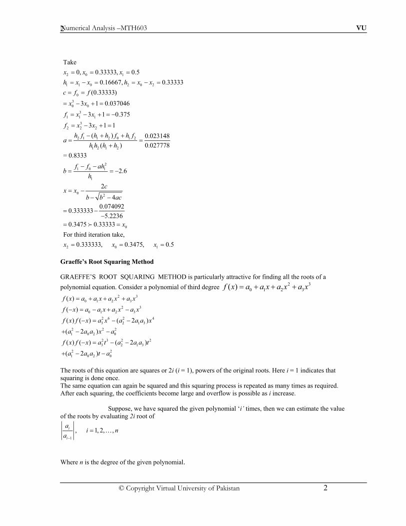
Take
0, 0.33333, 0.5
0.16667, 0.33333
(0.33333)
3 1 0.037046
3 1 0.375
3 1 1
( ) 0.023148
( ) 0.027778
= 0.8333
2
x x x
h x x h x x
c f f
x x
f x x
f x x
h f h h f h fa
h h h h
f f ahb
h
" " "
" " " "
" "
" ! "
" ! "
" ! "
! !" "
!
" "
02
0
2 0 1
.6
2
4
0.0740920.333333
5.2236
0.3475 0.33333
For third iteration take,
0.333333, 0.3475, 0.5
cx x
b b ac
x
x x x
"
"
" "
" " "
!
Graeffe’s Root Squaring Method
GRAEFFE’S ROOT SQUARING METHOD is particularly attractive for finding all the roots of a
polynomial equation. Consider a polynomial of third degree 2 3
0 1 2 3( )f x a a x a x a x" ! ! !
2 3
0 1 2 3
2 3
0 1 2 3
2 6 2 4
3 2 1 3
2 2 2
1 0 2 0
2 3 2 2
3 2 1 3
2 2
1 0 2 0
( )
( )
( ) ( ) ( 2 )
( 2 )
( ) ( ) ( 2 )
( 2 )
f x a a x a x a x
f x a a x a x a x
f x f x a x a a a x
a a a x a
f x f x a t a a a t
a a a t a
" ! ! !
" !
"
!
"
!
The roots of this equation are squares or 2i (i = 1), powers of the original roots. Here i = 1 indicates that
squaring is done once.
The same equation can again be squared and this squaring process is repeated as many times as required.
After each squaring, the coefficients become large and overflow is possible as i increase.
Suppose, we have squared the given polynomial ‘i’ times, then we can estimate the value
of the roots by evaluating 2i root of
1
, 1, 2, ,i
i
ai n
a
%%%%%% " "
Where n is the degree of the given polynomial.

Numerical Analysis –MTH603 VU
© Copyright Virtual University of Pakistan 3
3
The proper sign of each root can be determined by recalling the original equation. This method fails, when
the roots of the given polynomial are repeated.
This method has a great advantage over other methods in that it does not require prior information about
approximate values etc. of the roots. But it is applicable to polynomials only and it is capable of giving all
the roots. Let us see the case of the polynomial equation having real and distinct roots. Consider the
following polynomial equation 1 2
1 2 1
2 4 2 1 3 5 2
2 4 1 3 5
2
( ) ... 1)
( ...) ( ...)
n n n
n n
n n n n n n
f x x a x a x a x a
separating the even and odd powers of x and squaring we get
x a x a x a x a x a x
puttig x y and simplifying we get
" ! ! ! ! ! %%%%%%%%%%%%%%%%%&
% % % % % % % % % % % %
! ! ! " ! ! !
% " % % % % %
1 1 1
1 1 1
2 2
1 1
2
2 2 1 3 4
2
1 2
... 0 (2)
2
2 2
..... .... ...
( 1)
, ,... 1
n n n n
n
n
n n
n
the new equation
y b y b y b y b
b a a
b a a a a
b a
if p p p be the roots of eq then the roots of t
% % %
! ! ! ! ! " %%%%%%%%%%%%%%%%%%%%%
" !
" !
% %%%%%%%% %%%%%%%%%%%%%
"
% % % % % % % % % % % % 2 2 2
1 22 , ,... nhe equation are p p p% % % %%
Example
Using Graeffe root squaring method, find all the roots of the equation 3 26 11 6 0x x x ! "
Solution Using Graeffe root squaring method, the first three squared polynomials are as under:
For i = 1, the polynomial is
3 2
3 2
(36 22) (121 72) 36
14 49 36
x x x
x x x
!
" !
For i = 2, the polynomial is

Numerical Analysis –MTH603 VU
© Copyright Virtual University of Pakistan 4
4
3 2(196 98) (2401 1008) 1296
3 298 1393 1296
For i = 3, the polynomial is
3 2(9604 2786) (1940449 254016) 1679616
3 26818 16864333 1679616
The roots of polynomial are
36 490.85714, 1.8708,
49 14
x x x
x x x
x x x
x x x
!
" !
!
" !
" "
44 4
8
143.7417
1
; 2
1296 1393 980.9821, 1.9417, 3.1464
1393 98 1
Still better estimates of the roots obtained from polynomial (3) are
1679616 16864330.99949,
1686433 6818
Similarly the roots of the p oynomial are
"
% % % % % % % %
" " "
" 886818
1.99143, 3.01441
The exact values of the roots of the given polynomial are 1, 2 and 3.
" "
Example
Apply Graeffe,s root squaring method to solve the equation 3 28 17 10 0x x x ! "
Solution
3 2
2 2
( ) 8 17 10
, ,
( )
( 17) (8 10)
f x x x x
here three chnges are observed form ve to ve ve to ve ve to ve
hence according to deccarte rule of signs f x may have three positive roots
rewriting eq as x x x
" !
% % % % % %! % % % % %! % ! % % %
% % % % % % % % % % % % %
%% % % ! " !
2
2 2
3 2 2
2 2
2
2 2
3 2 2
2 2
( 17) (8 10)
34 289 64 160 100
( 129) 30 100
( 129) (30 100)
258 16641 900 6000 10000
( 16641) (642 10000
and squaring on both sides and putting x y
y y y
y y y y
y y y
putting y z we get
z z z
z z z z z
z z z
% % % % % % % "
! " !
! ! " ! !
! " !
% " % % %
! " !
! ! " ! !
! " !
2
2 2
3 2 2 8
3 2 8
)
( 16641) (642 10000)
33282 276922881 412164 12840000 10
378882 264082 10 0
squaring again and putting z u we get
u u u
u u u u u
u u u
% % % % " % % %
! " !
! ! " ! !
! "

Numerical Analysis –MTH603 VU
© Copyright Virtual University of Pakistan 5
5
1 2, 3, 1 2 3
1/ 8 1/ 8 1/ 8
1 1 1
1/ 8 1/ 8 1/ 8
2 2 2 1
1/ 8 1/ 8 8
3 3 3 2
1 , 5 , ,
( ) ( ) (378882) 4.9809593 5
( ) ( / ) (264082 / 378882) 0.9558821 1
( ) ( / ) (10 / 2
if the roots of the eq are p p p and those of eqiuation are q q q
p q
p q
p q
'
' '
' '
% % % % % % % % % % % % % %
" " " " (
" " " " (
" " " 1/ 864082) 2.1003064 2
(5) (2) (1) 0here f f f
hence all are the roots of the eqiuation
" (
% " " "
% % % % % % % %
Example
Find all the root of the equation 4 3 1 0x x ! "
Solution
Numerical Analysis –MTH603 VU
© Copyright Virtual University of Pakistan 6
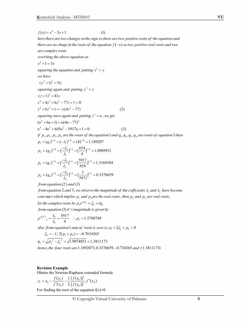
6
4( ) 3 1 (1)
( )
f x x x
here there are two changes in the sign so there are two positive roots of the equation and
there are no chnge in the roots of the equation f x so tw
" ! %%%%%%%%%%%%%%%%%%%%%%%%%%%%%%%%%%%
% % % % % % % % % % % % % % % % % %
% % % % % % % % % % % %
4
2
2 2
2
4 3 2
1 3
( 1) 9
81
4 6 77
o positive real roots and two
are complex roots
rewriting the above equation as
x x
squaring the equation and putting x y
we have
y y
squaring again and putting y z
z z
z z z
)
% % % % % %
% % %
% % % %
! "
% % % % % "
% %
%% ! "
% % % % " %
%& !*+ "
! !
4 2 2
2
2 2
4 3 2
1 2 3
1 0
6 1 (4 77) (2)
,
( 6 1) (4 77)
4 645 5917 1 0
, , ,
z
z z z z
squaring once again and putting z u we get
u u u u
u u u u
if p p p p
! "
! ! " %%%%%%%%%%%%%%%%%%%%%%%%%%%%%%%%%%%%%%%
% % % % % " % % %
! ! "
! ! " %%%%%%%%%%%%%%%%%%%%%%%%%%%%%%%%&,+
% 4 1 2 3 4
1/ 8 1/ 8 1/ 8
1 1 1
1/ 8 1/ 8 1/ 82
2 2
1
1/ 8 1/ 8 1/ 83
3 3
2
4
1 , , , 3
( ) ( ) (4) 1.189207
654( ) [ ] [ ] 1.8909921
4
5917( ) [ ] [ ] 1.3169384
654
are the roots of the equation and q q q q are roots of equation then
p q
p q
p q
p
'
'
'
'
'
% % % % % % % % % % % % % % %
" " " "
" " " "
" " " "
1/ 8 1/ 8 1/ 84
4
3
1 2
1 4
1( ) [ ] [ ] 0.3376659
5971
(2 ) (3)
2
tan
q
from equation and
from equation and we observe the magnitude of the cofficients and have become
cons t which implies p and p are the real
'
'
' '
" " " "
% % % % %
% % % %,%- % % % % % % % % % % % %
% % % % % % % %
2
3
2 3
2 2 2
2(2 ) 3
2 2
1
, ,
(3) '
59171.5780749
4
1
i
roots then p and p are real roots
let the complex roots be e i
from equation it s magnitude is given by
also from equation sum of roots is zero i
./ 0 1
'/ /
'
2
% % % % % % %
% % % % % " !
% % % % % % % %
" " %%%%$% "
% % % % % % % % % 2 4
2 1 4
2 2
2 2 2
. 2 0
1/ 2( ) 0.7634365
1.9074851 1.3811173
, 1.1892071,0.3376659, 0.734365 1.3811173
e p
p p
hence the four roots are and i
/ 0
0
1 / 0
*% ! ! " %
%%%%%%% " ! "
" " "
% % % % % %2
%
Revision Example Obtain the Newton-Raphson extended formula
2
0 0
1 0 03
0 0
( ) [ ( )]1( )
( ) 2 [ ( )]
f x f xx x f x
f x f x33"
3
For finding the root of the equation f(x)=0

Numerical Analysis –MTH603 VU
© Copyright Virtual University of Pakistan 7
7
Solution
Expanding f (x) by Taylor’s series and retaining up to second order term,
0 0 0
2
0
0
0 ( ) ( ) ( ) ( )
( )( )
2
f x f x x x f x
x xf x
3" " !
33!
Therefore,
1 0 1 0 0
2
1 0
0
( ) ( ) ( ) ( )
( )( ) 0
2
f x f x x x f x
x xf x
3" !
33! "
This can also be written as 2
0
0 1 0 0 02
0
[ ( )]1( ) ( ) ( ) ( ) 0
2 [ ( )]
f xf x x x f x f x
f x3 33! ! "
3
Thus, the Newton-Raphson extended formula is given by 2
0 0
1 0 03
0 0
( ) [ ( )]1( )
( ) 2 [ ( )]
f x f xx x f x
f x f x33"
3 3
This is also known as Chebyshev’s formula of third order

Numerical Analysis –MTH603 VU
© Copyright Virtual University of Pakistan 1
Solution of Linear System of Equations and Matrix Inversion
The solution of the system of equations gives n unknown values x1, x2, …, xn, which
satisfy the system simultaneously. If m > n, the system usually will have an infinite
number of solutions.
If 0A then the system will have a unique solution.
If 0,A !
Then there exists no solution.
Numerical methods for finding the solution of the system of equations are classified as
direct and iterative methods. In direct methods, we get the solution of the system after
performing all the steps involved in the procedure. The direct methods consist of
elimination methods and decomposition methods.
Under elimination methods, we consider, Gaussian elimination and Gauss-Jordan
elimination methods
Crout’s reduction also known as Cholesky’s reduction is considered under decomposition
methods.
Under iterative methods, the initial approximate solution is assumed to be known and is
improved towards the exact solution in an iterative way. We consider Jacobi, Gauss-
Seidel and relaxation methods under iterative methods.
Gaussian Elimination Method
In this method, the solution to the system of equations is obtained in two stages.
i) the given system of equations is reduced to an equivalent upper triangular form
using elementary transformations
ii) the upper triangular system is solved using back substitution procedure
This method is explained by considering a system of n equations in n unknowns in the
form as follows
11 1 12 2 1 1
21 1 22 2 2 2
1 1 2 2
.
.
n n
n n
n n nn n n
a x a x a x b
a x a x a x b
a x a x a x b
" " " ! #$" " " ! $$%$$
" " " ! $&
Stage I: Substituting the value of x1 from first equation into the rest
1 12 2 1 1
22 2 2 2
2 2
n n
n n
n nn n n
x a x a x b
a x a x b
a x a x b
' ' '" " " ! #$' ' '" " ! $%$$' ' '" " ! &
!

Numerical Analysis –MTH603 VU
© Copyright Virtual University of Pakistan 2
Now, the last (n – 1) equations are independent of x1, that is, x1 is eliminated from the
last (n – 1) equations.
This procedure is repeated and x2 is eliminated from 3rd, 4th, …, n-th equations
The same procedure is repeated till the given system assumes the upper triangular form:
11 1 12 2 1 1
22 2 2 2
n n
n n
nn n n
c x c x c x d
c x c x d
c x d
" " " ! #$(((( " " ! $%
(((((((((((((((((((((((((((((( $$(((((((((((((((((((((((( ! &
!
Stage II: The values of the unknowns are determined by backward substitution.
First xn is found from the last equation and then substitution this value of xn in the
preceding equation will give the value of xn-1. Continuing this way, we can find the
values of all other unknowns
Example
Solve the following system of equations using Gaussian elimination method
2 3 5
4 4 3 3
2 3 1
x y z
x y z
x y z
" ) !
" ) !
) " ) !
Solution
Stage I (Reduction to upper-triangular form):
Divide first equation by 2 and then subtract the resulting equation (multiplied by 4 and –
2) from the 2nd and 3rd equations respectively. Thus, we eliminate x from the 2nd and
3rd equations.
The resulting new system is given by
3 5
2 2 2
2 7
6 2 6
zx y
y z
y z
#" ) ! $$
() ) ! ) %$((( ) !$&
Now, we divide the 2nd equation by –2 and eliminate y from the last equation and the
modified system is given by
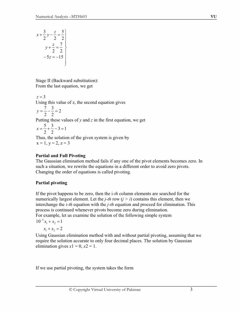
Numerical Analysis –MTH603 VU
© Copyright Virtual University of Pakistan 3
3 5
2 2 2
7
2 2
5 15
zx y
zy
z
#" ) ! $$$
(((((( " ! %$
((((() ! ) $$&
Stage II (Backward substitution):
From the last equation, we get
3z !
Using this value of z, the second equation gives
7 32
2 2y ! ) !
Putting these values of y and z in the first equation, we get
5 33 1
2 2x ! " ) !
Thus, the solution of the given system is given by
x = 1, y = 2, z = 3
Partial and Full Pivoting The Gaussian elimination method fails if any one of the pivot elements becomes zero. In
such a situation, we rewrite the equations in a different order to avoid zero pivots.
Changing the order of equations is called pivoting.
Partial pivoting
If the pivot happens to be zero, then the i-th column elements are searched for the
numerically largest element. Let the j-th row (j > i) contains this element, then we
interchange the i-th equation with the j-th equation and proceed for elimination. This
process is continued whenever pivots become zero during elimination.
For example, let us examine the solution of the following simple system 5
1 2
1 2
10 1
2
x x
x x
) " !
(((((( " !
Using Gaussian elimination method with and without partial pivoting, assuming that we
require the solution accurate to only four decimal places. The solution by Gaussian
elimination gives x1 = 0, x2 = 1.
If we use partial pivoting, the system takes the form

Numerical Analysis –MTH603 VU
© Copyright Virtual University of Pakistan 4
1 2
5
1 2
2
10 1
x x
x x)
" !
" !
Using Gaussian elimination method, the solution is found to be x1 = 1, x2 = 1, which
is a meaningful and perfect result.
In full pivoting (or complete pivoting), we interchange rows and columns, such that the
largest element in the matrix of the variables also get changed. Full pivoting, in fact, is
more complicated than the partial pivoting. Partial pivoting is preferred for hand
computation.
The general form of a system of m linear equations in n unknowns x1, x2, x3, …, xn can
be represented in matrix form as under:
11 12 13 1 1 1
21 22 23 2 2 2
1 2 3
n
n
m m m mn n m
a a a a x b
a a a a x b
a a a a x b
* + * + * +, - , - , -, - , - , -!, - , - , -, - , - , -. / . / . /
! ! ! ! ! !
Using matrix notation, the above system can be written in compact form as
[ ]( ) ( )A X B!
Note:
1. This method fails if any of he pivots become zero in such cases, by interchanging
the rows we can get the non-zero pivots.
Example
Solve the system of equations by Gaussian elimination method with partial pivoting.
7
3 3 4 24
2 3 16
x y z
x y z
x y z
" " !
" " !
" " !
Solution
1 1 1 7
3 3 4 24
2 1 3 16
x
y
z
* + 0 1 0 12 3 2 3, - !2 3 2 3, -2 3 2 3, -. / 4 5 4 5
To start with, we observe that the pivot element
11 1( 0).a !
However, a glance at the first column reveals that the numerically largest element is 3
which is in second row. Hence R12

Numerical Analysis –MTH603 VU
© Copyright Virtual University of Pakistan 5
Thus the given equation takes the form after partial pivoting
3 3 4 24
1 1 1 7
2 1 3 16
x
y
z
* + 0 1 0 12 3 2 3, - !2 3 2 3, -2 3 2 3, -. / 4 5 4 5
Stage I (Reduction to upper triangular form):
4 81 13
10 1 0
3
10 0 1
3
x
y
z
* + * + * +, - , - , -, - , - , -, - , - , -) !, - , - , -, - , - , -, -) , - , -). / . /, -. /
Stage II (Back substitution): 3
1 0 or 1
1 4 8 or 3
z
y y
x x
!
) " ! ((( ((( !
" " ! (( (( !
Example
Solve the following system of equations by Gaussian elimination method with partial
pivoting
1 2 3 4
1 2 3 4
1 2 3 4
1 2 3 4
0 4 2 8 24
4 10 5 4 32
4 5 6.5 2 26
9 4 4 0 21
x x x x
x x x x
x x x x
x x x x
" " " !
" " " !
" " " !
" " " !
Solution
In matrix notation, the given system can be written as
1
2
3
4
0 4 2 8 24
4 10 5 4 32
4 5 6.5 2 26
9 4 4 0 21
x
x
x
x
* +* + * +, -, - , -, -, - , -!, -, - , -, -, - , -
. / . /. /
To start with, we observe that the pivot row, that is, the first row has a zero pivot element
(a11 = 0). This row should be interchanged with any row following it, which on
becoming a pivot row should not have a zero pivot element.

Numerical Analysis –MTH603 VU
© Copyright Virtual University of Pakistan 6
While interchanging rows it is better to interchange the first and fourth rows, which is
called partial pivoting and get,
1
2
3
4
9 4 4 0 21
4 10 5 4 32
4 5 6.5 2 26
0 4 2 8 24
x
x
x
x
* +* + * +, -, - , -, -, - , -!, -, - , -, -, - , -
. / . /. /
Stage I (Reduction to upper-triangular form):
1
2
3
4
1
2
3
4
4 42.3331 0
9 922.6666
0 8.2222 3.2222 416.6666
0 3.2222 4.7222 224
0 4 2 8
4 42.3331 0
9 92.
0 1 0.3919 0.4865
0 0 3.4594 0.4324
0 0 0.4324 6.0540
x
x
x
x
x
x
x
x
* +* + * +, -, - , -, -, - , -!, -, - , -, -, - , -, - . /. /, -. /
* +* +, -, -, -, - !, -, -, -, -, - . /, -. /
1
2
3
4
7568
7.78836
12.9728
4 42.33331 0
9 92.7568
0 1 0.3919 0.48652.2500
0 0 1 0.125011.9999
0 0 0 5.999
x
x
x
x
* +, -, -, -, -. /
* +* + * +, -, - , -, -, - , -!, -, - , -, -, - , -, - . /. /, -. /
Stage II Back substitution
1 2 3 41.0, 1.0, 2.0, 2.0x x x x! ! ! !
Example
Solve the system of equations
3 3
2 8 5
2 9 8
x y z
x y z
x y z
" ) !
) " ! )
) " !
using Gauss elimination method.
Solution
The given system is equivalent to

Numerical Analysis –MTH603 VU
© Copyright Virtual University of Pakistan 7
3 1 1 3
2 8 1 5
1 2 9 8
arg
3 1 1 3
[ | ] 2 8 1 5
1 2 9 8
x
y
z
X B
the umented matrix is
A B
)* + * + * +, - , - , -) (( ! ), - , - , -, - , - , -). / . / . /(((((((((6((((((((((( ((!((
( ( ( (
)* +, -! ) ((7((() (, -, -). /
2 1 3 1
3 1 13
26 5 2 1~ 0 7 ,
3 3 3 37
7 280
3 3
26sin sec ,
3
3 1 13
26 5~ 0 7
3 3231
6930 0 26
78
now making as an upper triangular matrix
R R R R
now choo g as the pivot from the ond column
( (6( ( ( ( (
* +, -), -
), -((7((() (( ) ), -, -), -. /
)( ( ( ( ( ( ( ( (
* +, ),
), ((7((( ),,,.
2 1 3 1
2 1,
3 3
3 3
26 57
3 3
693 231
78 26
1
26 5 5 267 ( ) 7 (1) 1
3 3 3 3
1 1[3 ] [3 1 1] 1
3 3
1
R R R R
from this we get
x y z
y z
z
now by back substitution z
y z y
now x y z
so the solution is x y z
---(( ) )---/
( ( ( (
" ) !
)" ! )
!
( ( ( ( ! (
) )! ) ) ! ) ) ! 8 !
( ! ) " ! ) " !
( ( ( ( ! ! !
Example

Numerical Analysis –MTH603 VU
© Copyright Virtual University of Pakistan 8
Using Gauss elimination method, solve the system.
3.15 1.96 3.85 12.95
2.13 5.12 2.89 8.61
5.92 3.05 2.15 6.88
x y z
x y z
x y z
) " !
" ) ! )
" " !
Solution
The given system is equivalent to
3.15 1.96 3.85 12.95
2.13 5.12 2.89 8.61
5.92 3.05 2.15 6.88
x
y
z
A X
)* + * + * +, - , - , -) ((( (! ), - , - , -, - , - , -. / . / . /(((((((((((((((((( (((((((((((((((((((( ((!(((((9
2 1 3 1
3.15 1.96 3.85
[ | ] 2.13 5.12 2.89
5.92 3.05 2.15
3.15 1.96 3.852.13 5.92
~ 0 6.4453 5.4933 ,3.15 3.15
0 6.7335 5.0855
sin
A B
R R R R
choo g
) :;<=>* +, -! ) (((7(()?<@: (, -, -@<??. /) :;<=>* +
, -) (((7(():A<B@@A ((( ) ), -, -) ):A<C>A?. /
((@<CC>B
3 1
3.15 1.96 3.856.7335
~ 0 6.4453 5.49336.4453
0 0 0.6534
,
3.15 1.96 3.85 12.95
6.4453 5.4933 17.3667
0.6534 0.6853
as pivot
R R
form this we get
x y z
y z
z
by backward substit
(( ( (
) :;<=>* +, -) (((7(():A<B@@A ((( ), -, -D<@?>B. /
( ( ( (
) " !
) ! )
!
( (
0.68531.0488215
0.6534
5.4933 17.36671.8005692
6.4453
1.96 3.85 12.951.708864
3.15
ution
z
y
y zx
(
! !
)! ! )
) "! !
Example

Numerical Analysis –MTH603 VU
© Copyright Virtual University of Pakistan 9
Solve the system of equation
1 2 3 4
1 2 3 4
1 2 3 4
1 2 3 4
2
3 2 6
2 3 2 7
2 2
x x x x
x x x x
x x x x
x x x x
" " " !
" " ) ! )
" ) " !
" " ) ! )
By using Gauss elimination method.

Numerical Analysis –MTH603 VU
© Copyright Virtual University of Pakistan 10
1 2 3 4
1 2 3 4
1 2 3 4
1 2 3 4
1
2
3
4
2
3 2 6
2 3 2 7
2 2
1 1 1 1 2
1 1 3 2 6
2 3 1 2 7
1 2 1 1 2
x x x x
x x x x
x x x x
x x x x
the given system in matrix form is
x
x
x
x
A X
" " " !
" " ) ! )
" ) " !
" " ) ! )
( ( ( ( ( ( (
* +* + * +, -, - , -) ), -, - , -(!, -, - , -), -, - , -
) ). / . /. /(((( (((((((((((((((((((((((( (!((
2 1 3 1 4 1
1 1 1 1 2
1 1 3 2 6[ | ]
2 3 1 2 7
1 2 1 1 2
1 1 1 1 2
0 0 2 3 8~ , 2 ,
0 1 3 0 3
0 1 0 2 4
sin sec int
1 1 1 1
0 1~
B
A B
R R R R R R
ce the element in the ond column is zero so erchanging the rows
(
* +, -) ), -! ((((7((((, -), -
) ). /
* +, -) ), -((((7(((( ( ) ) ), -), -
) ). /( ( ( ( ( ( ( ( ( ( ( ( (
23
4 2
4 3
2
3 0 3
0 0 2 3 8
0 1 0 2 4
1 1 1 1 2
0 1 3 0 3~
0 0 2 3 8
0 1 3 2 4
2,
1 1 1 12
0 1 3 03 3
~ 0 0 2 38 2
550 0 0
2
R
R R
now the pivot is therefore
R R
* +, -), -((((7(((( (, -) ), -
) ). /
* +, -), -((((7(((( ( ), -) ), -
) ). /( ( ( ( (
* +, -), -
((((7(((( ( ), -)), -
, -, -. /

Numerical Analysis –MTH603 VU
© Copyright Virtual University of Pakistan 11
1 2 3 4
2 3
3 4
4
4
3 4
2 3
1 2 3 4
1 2 3 4
2
3 3
2 3 8
5( ) 52
2
1 1( 8 3 ) ( 8 6) 1
2 2
3 3 3 3 0
1
2 2 0 1 2 1
1, 0, 1, 2
from this we get
x x x x
x x
x x
x
now x
x x
now
x x
now from equation
x x x x
so x x x x
( ( ( (
" " " !
) !
) ! )
!
( !
! ) " ! ) " ! )
(
! " ! ) !
( ( ( (
! ) ) ) ! ) " ) !
( ! ! ! ) !

Numerical Analysis –MTH603 VU
© Copyright Virtual University of Pakistan 1
Solution of Linear System of Equations and Matrix Inversion
Gauss–Jordon Elimination Method
This method is a variation of Gaussian elimination method. In this method, the elements above and below
the diagonal are simultaneously made zero. That is a given system is reduced to an equivalent diagonal
form using elementary transformations. Then the solution of the resulting diagonal system is obtained. Sometimes, we normalize the pivot row with respect to the pivot element, before elimination. Partial
pivoting is also used whenever the pivot element becomes zero.
Example
Solve the system of equations using Gauss-Jordan elimination method:
2 8
2 3 4 20
4 3 2 16
x y z
x y z
x y z
! "#
! $# ! %
Solution
In matrix notation, the given system can be written as
1 2 1 8
2 3 4 20
4 3 2 16
1 2 1 8
0 1 2 4 (-2) R1 +R2 and (-4) R1+R3
0 5 2 16
Now, we eliminate y from the first and third rows using the seco
x
y
z
x
y
z
& ' ( ) ( )* + * +, - !* + * +, -* + * +, -. / 0 1 0 1
& ' ( ) ( )* + * +, -2 ! 33333333333* + * +, -* + * +, -2 2 2. / 0 1 0 1
nd row. Thus, we get
1 0 5 16
0 1 2 4
0 0 12 36
x
y
z
& ' ( ) ( )* + * +, -2 !* + * +, -* + * +, -2 2. / 0 1 0 1
Before, eliminating z from the first and second row, normalize the third row with respect to the pivot
element, we get
1 0 5 16
0 1 2 4
0 0 1 3
x
y
z
& ' ( ) ( )* + * +, -2 !* + * +, -* + * +, -. / 0 1 0 1
Using the third row of above Equation, and eliminating z from the first and second rows, we obtain
1 0 0 1
0 1 0 2
0 0 1 3
The solution is
x =1, y =2, z =3.
x
y
z
& ' ( ) ( )* + * +, -2 ! 2* + * +, -* + * +, -. / 0 1 0 1
Example
Solve the system of equation by using the Gauss Jordan elimination method 10 12
2 10 13
5 7
x y z
x y z
x y z
!
!
!
Solution
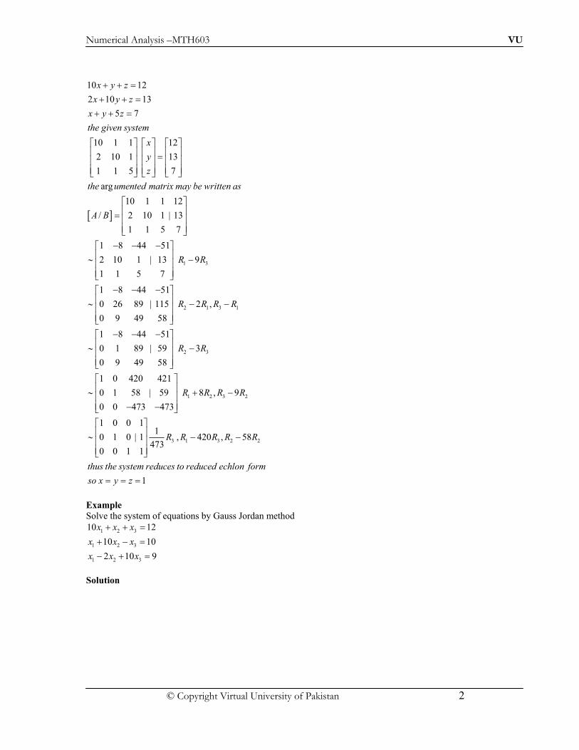
Numerical Analysis –MTH603 VU
© Copyright Virtual University of Pakistan 2
4 5
10 12
2 10 13
5 7
10 1 1 12
2 10 1 13
1 1 5 7
arg
10 1 1
/ 2 10 1
1 1 5
1 8 44
2 10 1
1 1 5
x y z
x y z
x y z
the given system
x
y
z
the umented matrix may be written as
A B
!
!
!
3 3 3
& ' & ' & ', - , - , -3 33 3!, - , - , -, - , - , -. / . / . /3 3 3 3 3 3 3
67& ', -! 3383369 3, -, -:. /
2 2 2;6
< 33833 69 1 3
2 1 3 1
2 3
1 2 3 2
9
1 8 44
0 26 89 2 ,
0 9 49
1 8 44
0 1 89 3
0 9 49
1 0 420
0 1 58 8 , 9
0 0 473
1 0 0
0 1 0 1
0 0 1
R R
R R R R
R R
R R R R
& ', -33 2, -, -:. /
2 2 2;6& ', -< 3383366; 33 2 2, -, -;=. /
2 2 2;6& ', -< 33833 ;> 33 2, -, -;=. /
?76& ', -< 33833 ;> 33 2, -, -2 2?:9. /
6& ', -< 33833, -, -6. /
3 1 3 2 2420 , 58
1
R R R R R
thus the system reduces to reduced echlon form
so x y z
63 3@ 2 2?:9
3 3 3 3 3 3 3 3
3 ! ! !
Example
Solve the system of equations by Gauss Jordan method
1 2 3
1 2 3
1 2 3
10 12
10 10
2 10 9
x x x
x x x
x x x
!
2 !
2 !
Solution

Numerical Analysis –MTH603 VU
© Copyright Virtual University of Pakistan 3
4 5
1 2 3
1 2 3
1 2 3
1
2
3
10 12
10 10
2 10 9
10 1 1 12
1 10 1 10
1 2 10 9
arg
10 1 1
/
x x x
x x x
x x x
the matrix form of the given system may be written as
x
x
x
the umented mairix may be written as
A B
!
2 !
2 !
3 3 3 3 3 3 3 3 3 3 3
& ' & ' & ', - , - , -2 33 3!, - , - , -, - , - , -2. / . / . /
3 3 3 3 3 3 3
!
1 2
2 1 3 1
32
1 10 1
1 2 10
1 89 10
~ 1 10 1 9
1 2 10
1 89 10
~ 0 9 1 ,
0 1 0
1 89 10
~ 0 9 1 ,99 87
0 1 0
1 89 10
~ 0 1 1
0 1 0
R R
R R R R
RR
67& ', -2 338336A 3, -, -2 >. /
2 2:=& ', -2 33833 == 33 2, -, -2 =:. /
2 2:=& ', -2 33833 = 33 2 2, -, -6. /
2 2:=& ', -2 33833 = 33, -, -6. /
2 2:=& ', 2 33833 A,, 6.
2 3
1 2 3 1
1 3 2 3
1 2 3
8
1 0 79
~ 0 1 1 89 ,
0 0 1
1 0 0
~ 0 1 1 1 79 ,
0 0 0
var
1
R R
R R R R
R R R R
so the system gives the values of all the three iables
x x x
-33 2--/
2 2:=& ', -2 33833 A 33 2 2, -, -6. /
6& ', -33833 33 , -, -6. /3 3 3 3 3 3 3 3 3 3 3
! ! !
Example
Solve the system of equations by using Gauss Jordan method.
2 2
2 3 2 7
3 2 6
2
x y z w
x y z w
x y z w
x y z w
2 ! 2
2 !
2 ! 2
!
Solution
2 2
2 3 2 7
3 2 6
2
x y z w
x y z w
x y z w
x y z w
2 ! 2
2 !
2 ! 2
!

Numerical Analysis –MTH603 VU
© Copyright Virtual University of Pakistan 4
1 2 1 1 2
2 3 1 2 7
1 1 3 2 6
1 1 1 1 2
the system may be written as
x
y
z
w
3 3 3 3 3 3
2 2& ' & ' & ', - , - , -2, - , - , -3333 33! 3, - , - , -2 2, - , - , -. / . / . /
4 5
2 1 3 1 4 1
arg
1 2 1 1
2 3 1 2/
1 1 3 2
1 1 1 1
1 2 1 1
0 1 3 42 , ,
0 1 2 1
0 1 0 2
1 0 5 7
0 1 3 4
0 0 1 1
0 0 3 2
the umented matrix may be written as
A B
R R R R R R
3 3 3 3 3 3 3
2 27& ', -2 :, -! 33833 333, -2 2B, -
7. /2 27& '
, -2 66, -< 33833 333 2 2 2, -2 2 2?, -
2 ?. /2 7A& '
, -2 266,< 33833, 2 29,
2 2:. /
1 2 3 2 4 2
1 3 2 3 4 3
1 4 2 4 3 4
12 , ( ),
5
1 0 0 2
0 1 0 15 , 3 , 3
0 0 1 1
0 0 0 1
1 0 0 0
0 1 0 02 , ,
0 0 1 0
0 0 0 1
1 0 0 0
0 1 0 0
0 0 1 0
0 0 0 1
R R R R R R
R R R R R R
R R R R R R
the system maybe written as
-333 2 --
;& ', -2 27, -< 33833 333 2 2, -2 29, -
7. /6& '
, -A, -< 33833 333 2 , -26, -
7. /3 3 3 3 3
&,
.
1, 0, 1, 2
x
y
z
w
the values of all the ariables are
x y z w
6' & ' & '- , - , -A, - , - , -3333 33! 3
, - , - , -26, - , - , -
7/ . / . /3 3 3 3 3 3 3
! ! ! 2 !
Crout’s ReductionMethod
Here the coefficient matrix [A] of the system of equations is decomposed into the product of two matrices
[L] and [U], where [L] is a lower-triangular matrix and [U] is an upper-triangular matrix with 1’s on its
main diagonal.
For the purpose of illustration, consider a general matrix in the form
4 54 5 4 5L U A!

Numerical Analysis –MTH603 VU
© Copyright Virtual University of Pakistan 5
11 12 13 11 12 13
21 22 23 21 22 23
31 32 33 31 32 33
0 0 1
0 0 1
0 0 1
l u u a a a
l l u a a a
l l l a a a
& ' & ' & ', - , - , -!, - , - , -, - , - , -. / . / . /
The sequence of steps for getting [L] and [U] are given below:
Step I: Multiplying all the rows of [L] by the first column of [U], we get
11 11 21 21 31 31, ,l a l a l a! ! !
Thus, we observe that the first column of [L] is same as the first column of [A].
Step II: Multiplying the first row of [L] by the second and third columns of [U], we obtain
11 12 12 11 13 13,l u a l u a! !
Or
1312
12 13
11 11
,aa
u ul l
! !
Thus, the first row of [U] is obtained. We continue this process, getting alternately the column of [L] and a
row of [U].
Step III: Multiply the second and third rows of [L] by the second column of [U] to get
21 12 22 22 31 12 32 32,l u l a l u l a ! !
This gives
22 22 21 12 32 32 31 12,l a l u l a l u! 2 ! 2
Step IV: Now, multiply the second row of [L] by the third column of [U] which yields
21 13 22 23 23
23 21 13
23
22
l u l u a
a l uu
l
!
2!
Step V: Lastly, we multiply the third row of [L] by the third column of [U] and get
31 13 32 23 33 33l u l u l a !
This gives
33 33 33 13 32 23l a l u l u! 2 2
Thus, the above five steps determine [L] and [U].
This algorithm can be generalized to any linear system of order n.
Consider a system of equations
11 1 12 2 13 3 1
21 1 22 2 23 3 2
31 1 32 2 33 3 3
a x a x a x b
a x a x a x b
a x a x a x b
! "#
! $# ! %
In matrix notation as [A](X) = (B). Let [A] = [L] [U], then we get,
[ ][ ]( ) ( )L U X B!
Substituting [U] (X) = (Z) in Eq. we obtain [L] (Z) = (B)
11 1 1
21 1 22 2 2
31 1 32 2 33 3 3
l z b
l z l z b
l z l z l z b
! "#
! $# ! %
Having computed z1, z2 and z3, we can compute x1, x2, and x3 from equation [U] (X) = (Z) or from
12 13 1 1
23 2 2
3 3
1
0 1
0 0 1
u u x z
u x z
x z
& ' ( ) ( )* + * +, - !* + * +, -* + * +, -. / 0 1 0 1
This method is also known as Cholesky reduction method. This technique is widely used in the numerical
solutions of partial differential equations.

Numerical Analysis –MTH603 VU
© Copyright Virtual University of Pakistan 6
This method is very popular from computer programming point of view, since the storages space reserved
for matrix [A] can be used to store the elements of [L] and [U] at the end of computation.
This method fails if any
0iia !
Example
Solve the following system of equations by Crout’s reduction method
1 2 3
1 2 3
1 2 3
5 2 4
7 5 8
3 7 4 10
x x x
x x x
x x x
2 !
2 !
!
Solution Let the coefficient matrix [A] be written as [L] [U]. Thus,
11 12 13
21 22 23
31 32 33
0 0 1 5 2 1
0 0 1 7 1 5
0 0 1 3 7 4
l u u
l l u
l l l
2& ' & ' & ', - , - , -! 2, - , - , -, - , - , -. / . / . /
Step I: Multiply all the rows of [L] by the first column of [U], we get
11 21 315, 7, 3l l l! ! !
Step II: Multiply the first row of [L] by the second and third columns of [U], we have
11 12 11 13
12 13
2, 1
2 1,
5 5
l u l u
u u
! 2 !
! 2 !
STEP III: Multiply the 2nd and 3rd rows of [L] by the 2nd column of [U], we get
21 12 22 22
31 12 32 32
14 191 1
5 5
6 417 7
5 5
l u l or l
l u l or l
" ! ! ! ##$# ! ! !#%
STEP IV: Multiply the 2nd row of [L] by the 3rd column of [U]
21 13 22 23
23
23
5
19 75
5 5
32
19
l u l u
u
u
! 2
! 2 2 333333333
! 2
STEP V: Finally, multiply the 3rd row of [L] with the 3rd column of [U], we obtain
31 13 32 23 33
33
4
327
19
l u l u l
l
!
!
Thus, the given system of equations takes the form [L][U][X] = (B).
1
2
3
2 1 415 0 0 5 5
19 327 0 0 1 8
5 19
41 327 0 0 13 10
5 19
x
x
x
& '& ' & ' & '2, -, - , - , -, -, - , - , -, -, - , - , -2 !, -, - , - , -, -, - , - , -, -, - , - , -. /. /, - , -. / . /
That is,

Numerical Analysis –MTH603 VU
© Copyright Virtual University of Pakistan 7
1
2
3
45 0 0
197 0 8
5
41 3273 10
5 19
z
z
z
& ' & ' & ', - , - , -, - , - , -, - , - , -!, - , - , -, - , - , -, - , - , -. /. /, -. /
Let [U](X) = (Z), then
[ ]( ) (4 8 10)TL Z !
Or
1
2
3
45 0 0
197 0 8
5
41 3273 10
5 19
z
z
z
& ' & ' & ', - , - , -, - , - , -, - , - , -!, - , - , -, - , - , -, - , - , -. /. /, -. /
Which gives utilizing these values of z, the Eq becomes
By back substitution method, we obtain
3 2 1
46 284 366, ,
327 327 327x x x! ! !
This is the required solution.
Example
Solve the following system
2 3 10 3
4 2 20
5 2 12
x y z
x y x
x y z
2 !
2 !
! 2
Solution
11 12 13
21 22 23
31 32 33
2 3 10 3
4 2 20
5 2 12
2 3 10
1 4 2
5 2 1
1 0 0
1 0 0
1 0 0
x y z
x y x
x y z
the given system is AX B
x
A X y
z
let LU A
u u u
L l U u u
l l u
2 !
2 !
! 2
3 3 3 3 !
2 9& ' & ' & ', - , - , -! 2 3333 !3 333333C ! 7A 33333, - , - , -, - , - , -267. / . / . /
3 !
& ' &, - ,!3 3333333 !3, -, -. / .
11 12 13
21 11 21 12 22 21 13 23
31 11 31 12 32 22 31 13 32 23 33
2 3 10
1 4 2
5 2 1
u u u
l u l u u l u u
l u l u l u l u l u u
'-33, -
, -/2& ' & '
, - , - ! 2, - , -, - , - . / . /

Numerical Analysis –MTH603 VU
© Copyright Virtual University of Pakistan 8
11 12 13
21 11 21
31 11 31
2 3 10
11
2
55
2
here
u u u
l u l
l u l
3
3
! 3@33 ! 2 333 !
2! 2 333D 3!
! 33333D3 !
21 12 22 22 21 12
21 13 23 23 21 13
31 12 32 22 32 31 12
22
31 13 32 23 33 33 31 13 32 23
1 54 4 4 ( )( 3)
2 2
12 2 2 ( )10 7
2
1 195 [5 ]
5
2531
5
1 0 0
11 0
2
5 191
2 5
l u u u l u
l u u u l u
l u l u l l uu
l u l u u u l u l u
L
2 ! 3333D ! 2 ! 2 2 !
2 ! 3333D ! 2 ! 2 !
! 3D ! 2 !
D ! 2 2 !
& ', -, -2, -! 33, -, -, -. /
1
2
3
1
2
3
2 3 10
50 7
2
2530 0
5
, ,
1 0 03
1. 1 0 20
212
5 191
2 5
1 0 0
11 0
2
5 191
2 5
U
y
let UX Y where y y then LY B
y
y
i e y
y
and
& ', -2, -, -33333333333333 !, -, -2, -. /
& ', -3 ! 333 3 ! 3 3 !, -, -. /
& ', -
& ' & ', -2 , - , -, -3 33 !, - , -, -
, - , -2, - . / . /, -. /3
& ', -, -2, -3 3, -, -, -. /
1
2
3
1
1 2 2
1 2 3 3
(1)
3
1 4320
2 2
5 19 50612
2 5 5
x y
y y
z y
now eqn implies
y
y y y
y y y y
& ' & ', - , -!3 3, - , -, - , -. / . /
3 3 3 3
! 33
2 ! 3D ! 3
2 ! 2 33D !

Numerical Analysis –MTH603 VU
© Copyright Virtual University of Pakistan 9
5 43 253 5062 3 10 3 , 7 ,
2 2 5 3
4, 3 2
x y z y z z
by back substitution x y and z
22 ! 33 ! 32 !
3 3 3 ! 2 ! 3 !
Example
Solve the following system 3 4 4
4 3 2
3 4 1
x y z
x y z
x y z
!
! 2
!
Solution
11 12 13
21 22 23
31 32 33
3 4 4
4 3 2
3 4 1
1 3 8
1 4 3
1 3 4
1 0 0
1 0 0
1 0 0
x y z
x y z
x y z
the given system is AX B
x
A X y
z
let LU A
u u u
L l U u u
l l u
u
!
! 2
!
3 3 3 3 !
?& ' & ' & ', - , - , -! 3333 !3 333333C ! 27 33333, - , - , -, - , - , -6. / . / . /
3 !
& ' & ', - , -!3 3333333 !3 33, - , -, - , -. / . /
11 12 13
21 11 21 12 22 21 13 23
31 11 31 12 32 22 31 13 32 23 33
1 3 8
1 4 3
1 3 4
u u
l u l u u l u u
l u l u l u l u l u u
& ' & ', - , - !, - , -, - , - . / . /
11 12 13
21 11 21
31 11 31
1 3 8
1 1
1 1
here
u u u
l u l
l u l
3
3
! 3@33 ! 333 !
! 2 333D 3!
! 33333D3 !

Numerical Analysis –MTH603 VU
© Copyright Virtual University of Pakistan 10
21 12 22 22 21 12
21 13 23 23 21 13
31 12 32 22 32 31 12
22
31 13 32 23 33 33 31 13 32 23
1 54 4 4 ( )( 3)
2 2
2 4 4 (1)3 1
13 [3 ] 0
4 4
1 0 0 1 3
1 1 0
1 0 1
l u u u l u
l u u u l u
l u l u l l uu
l u l u u u l u l u
L U
2 ! 3333D ! 2 ! 2 2 !
! 3333D ! 2 ! 2 !
! 3D ! 2 !
D ! 2 2 ! 2
& ', -! 3333333333333333 !, -, -. /
1
2
3
1
2
3
1
2
3
8
0 1 5
0 0 4
, ,
1 0 0 4
. 0 1 0 2
1 0 1 1
1 0 0
11 0
2
5 191
2 5
(1
y
let UX Y where y y then LY B
y
y
i e y
y
and
x y
y y
z y
now eqn
& ', -2, -, -2. /
& ', -3 ! 333 3 ! 3 3 !, -, -. /
& ' & ' & ', - , - , -3 33 ! 2, - , - , -, - , - , -. / . / . /3
& ', -
& ' & ', -2 , - , -, -3 3 !3 3, - , -, -
, - , -, - . / . /, -. /
3 3
1
2
1 3 3 1
)
4
2
1 1 3
3 8 4
5 2
4 3
3
4
3 72 5 2 5( )
4 4
7 3 294 3 8 4 3( ) 8( )
4 4 4
implies
y
y
y y y y
we also have
x y z
y z
z
by back substitutiton
z
y z
x y z
3 3
! 33
! 2
! 33D ! 2 ! 2
3 3 3
!
2 ! 2
2 ! 2
3 3 3
!
! 2 ! 2 !
! 2 2 ! 2 2 !

Numerical Analysis –MTH603 VU
© Copyright Virtual University of Pakistan 1
Solution of Linear System of Equationsand Matrix Inversion
Jacobi’s Method
This is an iterative method, where initial approximate solution to a given system of
equations is assumed and is improved towards the exact solution in an iterative way.
In general, when the coefficient matrix of the system of equations is a sparse matrix
(many elements are zero), iterative methods have definite advantage over direct methods
in respect of economy of computer memory
Such sparse matrices arise in computing the numerical solution of partial differential
equations
Let us consider
11 1 12 2 1 1
21 1 22 2 2 2
1 1 2 2 1
n n
n n
n n nn n
a x a x a x b
a x a x a x b
a x a x a x b
! "# ! #$## ! %
! ! ! !
In this method, we assume that the coefficient matrix [A] is strictly diagonally dominant,
that is, in each row of [A] the modulus of the diagonal element exceeds the sum of the
off-diagonal elements.
We also assume that the diagonal element do not vanish. If any diagonal element
vanishes, the equations can always be rearranged to satisfy this condition.
Now the above system of equations can be written as
11 121 2
11 11 11
22 212 1
22 22 22
( 1)11 1
nn
nn
n nn nn n
nn nn nn
ab ax x x
a a a
ab ax x x
a a a
ab ax x x
a a a
&&
"! & & & #
##
! & & & #$###
! & & & #%
! ! ! !
We shall take this solution vector 1 2( , ,..., )T
nx x x as a first approximation to the exact
solution of system. For convenience, let us denote the first approximation vector by (1) (1) (1)
1 2( , ,..., )nx x x got after taking as an initial starting vector.
Substituting this first approximation in the right-hand side of system, we obtain the
second approximation to the given system in the form

Numerical Analysis –MTH603 VU
© Copyright Virtual University of Pakistan 2
(2) (1) (1)11 121 2
11 11 11
(2) (1) (1)22 212 1
22 22 22
( 1)(2) (1) (1)11 1
nn
nn
n nn nn n
nn nn nn
ab ax x x
a a a
ab ax x x
a a a
ab ax x x
a a a
&&
"! & & & #
##
! & & & #$###
! & & & #%
! ! ! !
This second approximation is substituted into the right-hand side of Equations and obtain
the third approximation and so on.
This process is repeated and (r+1)th approximation is calculated
( 1) ( ) ( )11 121 2
11 11 11
( 1) ( ) ( )22 212 1
22 22 22
( 1)( 1) ( ) ( )11 1
r r rnn
r r rnn
n nr r rn nn n
nn nn nn
ab ax x x
a a a
ab ax x x
a a a
ab ax x x
a a a
& &
"! & & & #
##
! & & & #$###
! & & & #%
! ! ! !
Briefly, we can rewrite these Equations as
( 1) ( )
1
,
1, 2,..., 1, 2,...,
nijr ri
i j
jii iij i
abx x
a a
r i n
!'
! &
! !
(
It is also known as method of simultaneous displacements,
since no element of ( 1)r
ix is used in this iteration until every element is computed.
A sufficient condition for convergence of the iterative solution to the exact solution is
11
, 1, 2,...,n
ii ij
jj
a a i n!'
) !( When this condition (diagonal dominance) is true, Jacobi’s
method converges
Example
Find the solution to the following system of equations using Jacobi’s iterative method for
the first five iterations:
83 11 4 95
7 52 13 104
3 8 29 71
x y z
x y z
x y z
& !
!
!
Solution

Numerical Analysis –MTH603 VU
© Copyright Virtual University of Pakistan 3
95 11 4
83 83 83
104 7 13
52 52 52
71 3 8
29 29 29
x y z
y x z
z x y
"! & ###
! & & $##
! & & #%
Taking the initial starting of solution vector as (0,0,0) ,T from Eq. ,we have the first
approximation as
(1)
(1)
(1)
1.1446
2.0000
2.4483
x
y
z
* + * +, - , -!, - , -
, -, - . /. /
Now, using Eq. ,the second approximation is computed from the equations
(2) (1) (1)
(2) (1) (1)
(2) (1) (1)
1.1446 0.1325 0.0482
2.0 0.1346 0.25
2.4483 0.1035 0.2759
x y z
y x z
z x y
"! & #
! & & $#! & & %
Making use of the last two equations we get the second approximation as (2)
(2)
(2)
0.9976
1.2339
1.7424
x
y
z
* + * +, - , -!, - , -
, -, - . /. /
Similar procedure yields the third, fourth and fifth approximations to the required
solution and they are tabulated as below;
Variables
Iteration number r x y z
1 1.1446 2.0000 2.4483
2 0.9976 1.2339 1.7424
3 1.0651 1.4301 2.0046
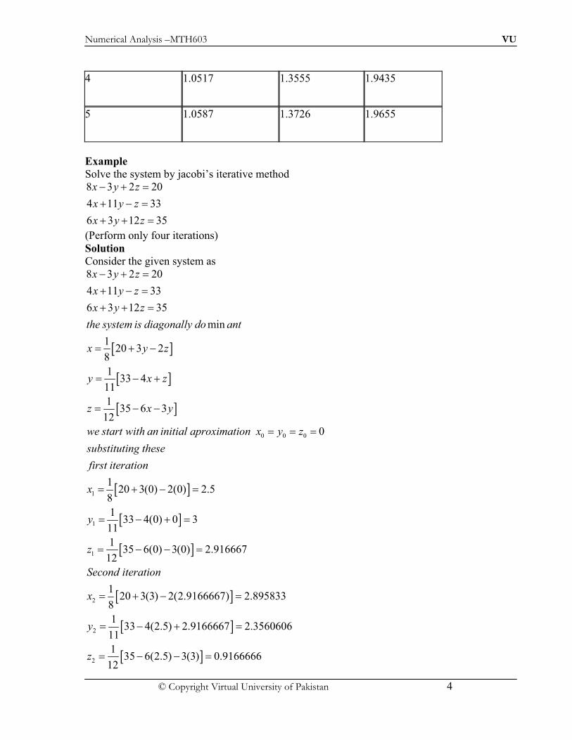
Numerical Analysis –MTH603 VU
© Copyright Virtual University of Pakistan 4
4 1.0517 1.3555 1.9435
5 1.0587 1.3726 1.9655
Example
Solve the system by jacobi’s iterative method
8 3 2 20
4 11 33
6 3 12 35
x y z
x y z
x y z
& !
& !
!
(Perform only four iterations)
Solution
Consider the given system as
0 1
0 1
0 1
0 0 0
1
8 3 2 20
4 11 33
6 3 12 35
min
120 3 2
8
133 4
11
135 6 3
12
0
120 3(0)
8
x y z
x y z
x y z
the system is diagonally do ant
x y z
y x z
z x y
we start with an initial aproximation x y z
substituting these
first iteration
x
& !
& !
!
2 2 2 2
! &
! &
! & &
2 2 2 2 2 22 ! ! !
2 2
2 2
! 0 1
0 1
0 1
0 1
0 1
0 1
1
1
2
2
2
2(0) 2.5
133 4(0) 0 3
11
135 6(0) 3(0) 2.916667
12
120 3(3) 2(2.9166667) 2.895833
8
133 4(2.5) 2.9166667 2.3560606
11
135 6(2.5) 3(3) 0.9166666
12
y
z
Second iteration
x
y
z
& !
! & !
! & & !
2 2
! & !
! & !
! & & !

Numerical Analysis –MTH603 VU
© Copyright Virtual University of Pakistan 5
0 1
0 1
0 1
3
3
3
120 3(2.3560606) 2(0.9166666) 3.1543561
8
133 4(2.8958333) 0.9166666 2.030303
11
135 6(2.8958333) 3(2.3560606) 0.8797348
12
third iteration
x
y
z
2 2
! & !
! & !
! & & !
0 1
0 1
0 1
4
4
4
120 3(2.030303) 2(0.8797348) 3.0419299
8
133 4(3.1543561) 0.8797348 1.9329373
11
135 6(3.1543561) 3(2.030303) 0.8319128
12
fourth iteration
x
y
z
22 22
! & !
! & !
! & & !
Example
Solve the system by jacobi’s iterative method
3 4 15 54.8
12 3 39.66
10 2 7.74
x y z
x y z
x y z
!
!
& !
(Perform only four iterations)
Solution
Consider the given system as
0 1
0 1
0 1
3 4 15 54.8
12 3 39.66
10 2 7.74
min
10 2 7.74
12 3 39.66
3 4 15 54.8
17.74 2
10
139.66 3
12
154.8 3 4
15
x y z
x y z
x y z
the system is not diagonally do ant we rearrange the system
x y z
x y z
x y z
x y z
y x z
z x y
!
!
& !
2 2 2 2 2 2 2 2 2 2
& !
!
!
! &
! & &
! & &

Numerical Analysis –MTH603 VU
© Copyright Virtual University of Pakistan 6
0 1
0 1
0 1
0 0 0
1
1
1
2
0
17.74 (0) 2(0) 0.774
10
139.66 (0) 3(0) 1.1383333
12
154.8 3(0) 4(0) 3.6533333
15
17.74 1.1
10
we start with an initial aproximation x y z
substituting these
first iteration
x
y
z
Second iteration
x
2 2 2 2 2 22 ! ! !
2 2
2 2
! & !
! & & !
! & & !
2 2
! &0 1
0 1
0 1
2
2
383333 2(3.6533333) 1.3908333
139.66 0.774 3(3.6533333) 2.3271667
12
154.8 3(0.774) 4(1.1383333) 3.1949778
15
y
z
!
! & & !
! & & !
0 1
0 1
0 1
3
3
3
17.74 2.3271667 2(3.1949778) 1.1802789
10
139.66 1.3908333 3(3.1949778) 2.3903528
12
154.8 3(1.3908333) 4(2.3271667) 2.7545889
15
third iteration
x
y
z
2 2
! & !
! & & !
! & & !
0 1
0 1
0 1
4
4
4
17.74 2.5179962 2(2.7798501) 1.0781704
10
139.66 1.1802789 3(2.7545889) 2.51779962
12
154.8 3(1.1802789) 4(2.3903528) 2.7798501
15
fourth iteration
x
y
z
2 22
! & !
! & & !
! & & !

Numerical Analysis –MTH603 VU
© Copyright Virtual University of Pakistan 1
Solution of Linear System of Equations and Matrix Inversion
Gauss–Seidel Iteration Method
It is another well-known iterative method for solving a system of linear equations of the
form
11 1 12 2 1 1
21 1 22 2 2 2
1 1 2 2
n n
n n
n n nn n n
a x a x a x b
a x a x a x b
a x a x a x b
! "# ! #$## ! %
! ! ! !
In Jacobi’s method, the (r + 1)th approximation to the above system is given by
Equations
( 1) ( ) ( )11 121 2
11 11 11
( 1) ( ) ( )22 212 1
22 22 22
( 1)( 1) ( ) ( )11 1
r r rnn
r r rnn
n nr r rn nn n
nn nn nn
ab ax x x
a a a
ab ax x x
a a a
ab ax x x
a a a
& &
"! & & & #
##
! & & & #$###
! & & & #%
! ! ! !
Here we can observe that no element of ( 1)r
ix replaces ( )r
ix entirely for the next cycle of
computation.
In Gauss-Seidel method, the corresponding elements of ( 1)r
ix replaces those of
( )r
ix as soon as they become available.
Hence, it is called the method of successive displacements. For illustration consider
11 1 12 2 1 1
21 1 22 2 2 2
1 1 2 2
n n
n n
n n nn n n
a x a x a x b
a x a x a x b
a x a x a x b
! "# ! #$## ! %
! ! ! !
In Gauss-Seidel iteration, the (r + 1)th approximation or iteration is computed from:
( 1) ( ) ( )11 121 2
11 11 11
( 1) ( 1) ( )22 212 1
22 22 22
( 1)( 1) ( 1) ( 1)11 1
r r rnn
r r rnn
n nr r rn nn n
nn nn nn
ab ax x x
a a a
ab ax x x
a a a
ab ax x x
a a a
& &
"! & & & #
##
! & & & #$###
! & & & #%
! ! ! !
Thus, the general procedure can be written in the following compact form

Numerical Analysis –MTH603 VU
© Copyright Virtual University of Pakistan 2
1( 1) ( 1) ( )
1 1
i nij ijr r ri
i j j
j j iii ii ii
a abx x x
a a a
&
! !
! & &' ' for all 1,2,...,i n! and 1,2,...r !
To describe system in the first equation, we substitute the r-th approximation into the
right-hand side and denote the result by ( 1)
1 .rx In the second equation, we substitute ( 1) ( ) ( )
1 3( , ,..., )r r r
nx x x and denote the result by ( 1)
2
rx
In the third equation, we substitute ( 1) ( 1) ( ) ( )
1 2 4( , , ,..., )r r r r
nx x x x and denote the result by ( 1)
3 ,rx and so on. This process is continued till we arrive at the desired result. For
illustration, we consider the following example :
Note
The difference between jacobi’s method and gauss Seidel method is that in jacobi’s
method the approximation calculated are used in the next iteration for next
approximation but in Gauss-seidel method the new approximation calculated is
instantly replaced by the previous one.
Example
Find the solution of the following system of equations using Gauss-Seidel method and
perform the first five iterations:
1 2 3
1 2 4
1 3 4
2 3 4
4 2
4 2
4 1
4 1
x x x
x x x
x x x
x x x
& & !
& & !
& & !
& & !
Solution
The given system of equations can be rewritten as
1 2 3
2 1 4
3 1 4
4 2 3
0.5 0.25 0.25
0.5 0.25 0.25
0.25 0.25 0.25
0.25 0.25 0.25
x x x
x x x
x x x
x x x
! "#! #$
! ##! %
Taking 2 3 4 0x x x! ! ! on the right-hand side of the first equation of the system , we get (1)
1 0.5.x ! Taking 3 4 0x x! ! and the current value of 1,x we get from the 2nd equation
of the system (1)
2 0.5 (0.25)(0.5) 0 0.625x ! !
Further, we take x4 = 0 and the current value of x1 we obtain from the third equation of
the system
(1)
3 0.25 (0.25)(0.5) 0
0.375
x !
!

Numerical Analysis –MTH603 VU
© Copyright Virtual University of Pakistan 3
Now, using the current values of x2 and x3 the fourth equation of system gives (1)
4 0.25 (0.25)(0.625)
(0.25)(0.375) 0.5
x !
!
The Gauss-Seidel iterations for the given set of equations can be written as ( 1) ( ) ( )
1 2 3
( 1) ( 1) ( )
2 1 4
( 1) ( 1) ( )
3 1 4
( 1) ( 1) ( 1)
4 2 3
0.5 0.25 0.25
0.5 0.25 0.25
0.25 0.25 0.25
0.25 0.25 0.25
r r r
r r r
r r r
r r r
x x x
x x x
x x x
x x x
!
!
!
!
Now, by Gauss-Seidel procedure, the 2nd and subsequent approximations can be
obtained and the sequence of the first five approximations are tabulated as below:
Variables
Iteration
number r
x1 x2 x3 x4
1 0.5 0.625 0.375 0.5
2 0.75 0.8125 0.5625 0.59375
3 0.84375 0.85938 0.60938 0.61719
4 0.86719 0.87110 0.62110 0.62305
5 0.87305 0.87402 0.62402 0.62451
Example
Solve the system by Gauss-Seidel iterative method 8 3 2 20
4 11 33
6 3 12 35
x y z
x y z
x y z
& !
& !
!
(Perform only four iterations)
Solution
Consider the given system as

Numerical Analysis –MTH603 VU
© Copyright Virtual University of Pakistan 4
( )
( )
( )
0 0 0
1
8 3 2 20
4 11 33
6 3 12 35
min
120 3 2
8
133 4
11
135 6 3
12
0
120 3(0)
8
x y z
x y z
x y z
the system is diagonally do ant
x y z
y x z
z x y
we start with an initial aproximation x y z
substituting these
first iteration
x
& !
& !
!
* * * *
! &
! &
! & &
* * * * * ** ! ! !
* *
* *
! ( )
( )
( )
( ) ( )
( ) ( )
1
1
2 1 1
2 2 1
2(0) 2.5
133 4(2.5) 0 2.0909091
11
135 6(2.5) 3(2.0909091) 1.1439394
12
1 120 3 20 3(2.0909091) 2(1.1439394) 2.9981061
8 8
1 133 4 33 4(2.9981061) 1.1439394 2.0137741
11 11
y
z
Second iteration
x y z
y x z
& !
! & !
! & & !
* *
! & ! & !
! & ! & !
( ) ( )2 2 2
1 135 6 3 35 6(2.9981061) 3(2.0137741) 0.9141701
12 12z x y! & & ! & & !
( )
( )
( )
3
3
3
120 3(2.0137741) 2(0.9141701) 3.0266228
8
133 4(3.0266228) 0.9141701 1.9825163
11
135 6(3.0266228) 3(1.9825163) 0.9077262
12
third iteration
x
y
z
* *
! & !
! & !
! & & !
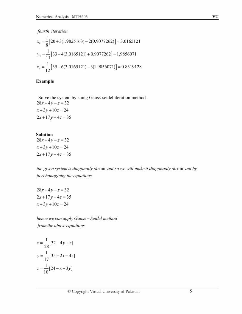
Numerical Analysis –MTH603 VU
© Copyright Virtual University of Pakistan 5
( )
( )
( )
4
4
4
120 3(1.9825163) 2(0.9077262) 3.0165121
8
133 4(3.0165121) 0.9077262 1.9856071
11
135 6(3.0165121) 3(1.9856071) 0.8319128
12
fourth iteration
x
y
z
** **
! & !
! & !
! & & !
Example
Solve the system by suing Gauss-seidel iteration method
28 4 32
3 10 24
2 17 4 35
x y z
x y z
x y z
& !
!
!
Solution
28 4 32
3 10 24
2 17 4 35
min min
28 4 32
2 17 4 35
3 10 24
x y z
x y z
x y z
the given system is diagonally do ant so we will make it diagonaaly do ant by
iterchanaginhg the equations
x y z
x y z
x y z
hence we can apply Gau
& !
!
!
* * * * * * * * * * * * * *
* *
& !
!
!
* * * *
1[32 4 ]
28
1[35 2 4 ]
17
1[24 3 ]
10
ss Seidel method
from the above equations
x y z
y x z
z x y
& * *
* * * *
! &
! & &
! & &

Numerical Analysis –MTH603 VU
© Copyright Virtual University of Pakistan 6
1
1
1
0
1[32] 1.1428571
28
1.1428571 , 0
1[35 2(1.1428571) 4(0)] 1.9243697
17
1.1428571 1.9243697
1[24 1.1428571 3(1.9243697)] 1.7084034
10
First approximation
putting y z
x
puting x z
y
putting x y
z
Second
* *
* ! !
! !
* ! *** ! *
! & & !
* ! **+* !
! & & !
2
2
2
3
1[32 4(1.9243697) 1.7084034] 0.9289615
28
1[35 2(0.9289615) 4(1.7084034)] 1.5475567
17
1[24 0.9289615 3(1.5475567)] 1.8408368
10
1[32 4(1.5475567) 1.8428368] 0.98759
28
iteration
x
y
z
third iteration
x
* *
! & !
! & & !
! & & !
* *
! & !
3
3
4
4
4
32
1[35 2(0.9875932) 4(1.8428368)] 1.5090274
17
1[24 0.9875932 3(1.5090274)] 1.8485325
10
1[32 4(1.5090274) 1.8485325] 0.9933008
28
1[35 2(0.9933008) 4(1.8428368)] 1.5070158
17
y
z
fourth iteration
x
y
z
! & & !
! & & !
* *
! & !
! & & !
!1
[24 0.9933008 3(1.5070158)] 1.848565210
& & !
Example
Using Gauss-Seidel iteration method, solve the system of the equation. 10 2 3
2 10 15
10 2 27
2 10 9
x y z w
x y z w
x y z w
x y z w
& & & !
& & & !
& & & !
& & & ! &

Numerical Analysis –MTH603 VU
© Copyright Virtual University of Pakistan 7
(Perform only four iterations)
Solution 10 2 3
2 10 15
10 2 27
2 10 9
min
1[3 2 ]
10
1[15 2 ]
10
1[27 2 ]
10
1[ 9 2 ]
10
x y z w
x y z w
x y z w
x y z w
it is diagonally do anat and we may write eqaution as
x y z w
y x z w
z x y w
w x y z
first approximation
putting
& & & !
& & & !
& & & !
& & & ! &
* * * * * * * * * *
!
!
!
! &
* *
1
1
1
1
2
0 (1) ,
0.3
1[15 2(0.3)] 1.56
10
0.3, 1.56 0
1[27 0.3 1.56] 2.886
10
0.3, 1.56 2.886
1[ 9 0.3 1.56 2(2.886)] 0.1368
10
sec
y z w on RHS of we get
x
y
putting x y and w
z
putting x y and z
w
ond iteration
x
* ! ! ! * * * * * * *
!
! !
** ! ! * * !
! !
* ! ! * * !
! & ! &
* *
2
2
2
3
1[3 2(1.56) 2.886 0.1368] 0.88692
10
1[15 2(0.88692) 2.886 0.1368] 1.952304
10
1[27 0.88692 1.952304 2( 0.1368)] 2.9565624
10
1[ 9 0.88692 1.952304 2(2.9565624)] 0.0247651
10
1
10
y
z
w
third iteration
x
! & !
! & !
! & !
! & ! &
* *
! [3 2(1.952304) 2.9565624 0.0.0247651] 0.9836405 & !

Numerical Analysis –MTH603 VU
© Copyright Virtual University of Pakistan 8
3
3
3
4
1[15 2(0.9836405) 2.9565624 0.0247651] 1.9899087
10
1[27 0.9836405 1.9899087 2( 0.0247651)] 2.9924019
10
1[ 9 0.983405 1.9899087 2(2.9924019)] 0.0041647
10
1[3 2(1.9899087) 2
10
y
z
w
fourth iteration
x
! & !
! & !
! & ! &
* *
!
4
4
4
.9924019 0.0041647] 0.9968054
1[15 2(0.9968054) 2.9924019 0.0041647] 1.9981848
10
1[27 0.9968054 1.9981848 2( 0.0041647)] 2.9986661
10
1[ 9 0.9968054 1.9981848 2(2.9986661)] 0.0007677
10
y
z
w
& !
! & !
! & !
! & ! &
Note
When to stop the iterative processes ,we stop the iterative process when we get the
required accuracy means if your are asked that find the accurate up to four places of
decimal then we will simply perform up to that iteration after which we will get the
required accuracy. If we calculate the root of the equation and its consecutive values are
1.895326125, 1.916366125, 1.919356325, 1.919326355, 1.919327145, 1.919327128
Here the accuracy up to seven places of decimal is achieved so if you are asked to acquire
the accuracy up to six places of decimal then we will stop here .
But in the solved examples only some iteration are carried out and accuracy is not
considered here.

Numerical Analysis –MTH603 VU
© Copyright Virtual University of Pakistan 1
Solution of Linear System of Equations and Matrix Inversion
Relaxation Method This is also an iterative method and is due to Southwell.To explain the details, consider again the system of equations
11 1 12 2 1 1
21 1 22 2 2 2
1 1 2 2
n n
n n
n n nn n n
a x a x a x b
a x a x a x b
a x a x a x b
! "# ! #$## ! %
! ! ! !
Let ( ) ( ) ( ) ( )
1 2( , ,..., )p p p p T
nX x x x!
be the solution vector obtained iteratively after p-th iteration. If ( )p
iR denotes the
residual of the i-th equation of system given above , that is of 1 1 2 2i i in n ia x a x a x b !
defined by ( ) ( ) ( ) ( )
1 1 2 2p p p p
i i i i in nR b a x a x a x! & & & &
we can improve the solution vector successively by reducing the largest residual to zero at that iteration. This is the basic idea of relaxation method. To achieve the fast convergence of the procedure, we take all terms to one side and then reorder the equations so that the largest negative coefficients in the equations appear on the diagonal. Now, if at any iteration, iR is the largest residual in magnitude, then we give an
increment to ;ix iia being the coefficient of xi
ii
ii
Rdx
a!
In other words, we change .ix to ( )i ix dx to relax iR that is to reduce iR to zero.
Example
Solve the system of equations
1 2 3
1 2 3
1 2 3
6 3 11
2 8 15
7 10
x x x
x x x
x x x
& !
& ! &
& !
by the relaxation method, starting with the vector (0, 0, 0).
Solution
At first, we transfer all the terms to the right-hand side and reorder the equations, so that the largest coefficients in the equations appear on the diagonal.

Numerical Analysis –MTH603 VU
© Copyright Virtual University of Pakistan 2
Thus, we get
1 2 3
1 2 3
1 2 3
0 11 6 3
0 10 7
0 15 2 8
x x x
x x x
x x x
! & & "#
! & & $#! & & & %
after interchanging the 2nd and 3rd equations. Starting with the initial solution vector (0, 0, 0), that is taking 1 2 3 0,x x x! ! !
we find the residuals 1 2 311, 10, 15R R R! ! ! &
of which the largest residual in magnitude is R3, i.e. the 3rd equation has more error and needs immediate attention for improvement. Thus, we introduce a change, dx3in x3 which is obtained from the formula
33
33
151.875
8
Rdx
a! & ! !
Similarly, we find the new residuals of large magnitude and relax it to zero, and so on. We shall continue this process, until all the residuals are zero or very small. Iteration Residuals Maximum Difference Variables
number R1 R2 R3 iR idx x1 x2 x3
0 11 10 -15 -15 1.875 0 0 0
1 9.125 8.125 0 9.125 1.5288 0 0 1.875
2 0.0478 6.5962 -
3.0576 6.5962 -0.9423 1.5288 0 1.875
Iteration Residuals Maximum Difference Variables

Numerical Analysis –MTH603 VU
© Copyright Virtual University of Pakistan 3
number R1 R2 R3 ! ! ! ! ! ! ! ! ! ! Ü ! ! ! ! ! ! ! ! ! ! Ü x1 x2 x3
0 11 10 -15 -15 15/8
=1.875 0 0 0
1 9.125 8.125 0 9.125 -9.125/(-6)
=1.5288 0 0 1.875
2 0.0478 6.5962 -
3.0576
6.5962 -6.5962/7
=-0.9423 1.5288 0 1.875
3 -
2.8747 0.0001 -
2.1153
-2.8747 2.8747/(-6)
=-0.4791 1.0497 -
0.9423
1.875
4 -
0.0031 0.4792 -
1.1571
-1.1571 1.1571/8
=0.1446 1.0497 -
0.9423
1.875
Iteration Residuals Maximum Difference Variables
number R1 R2 R3 ! ! ! ! ! ! ! ! ! ! Ü ! ! ! ! ! ! ! ! ! ! Ü x1 x2 x3
5 -
0.1447 0.3346 0.0003 0.3346 -.3346/7
=-0.0478 1.0497 -
0.9423
2.0196
6 0.2881 0.0000 0.0475 0.2881 -.2881/(-6)
=0.0480 1.0497 -
0.9901
2.0196
7 -
0.0001 0.048 0.1435 0.1435 =-0.0179 1.0017 -
0.9901
2.0196
8 0.0178 0.0659 0.0003 - - 1.0017 -
0.9901
2.0017
At this stage, we observe that all the residuals R1, R2 and R3 are small enough and therefore we may take the corresponding values of xi at this iteration as the solution. Hence, the numerical solution is given by
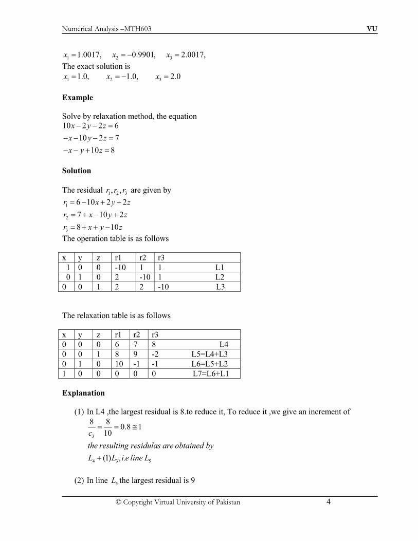
Numerical Analysis –MTH603 VU
© Copyright Virtual University of Pakistan 4
1 2 31.0017, 0.9901, 2.0017,x x x! ! & !
The exact solution is
1 2 31.0, 1.0, 2.0x x x! ! & !
Example
Solve by relaxation method, the equation 10 2 2 6
10 2 7
10 8
x y z
x y z
x y z
& & !
& & & !
& & !
Solution
The residual 1 2 3, ,r r r are given by
1
2
3
6 10 2 2
7 10 2
8 10
r x y z
r x y z
r x y z
! &
! &
! &
The operation table is as follows x y z r1 r2 r3 1 0 0 -10 1 1 L1 0 1 0 2 -10 1 L2 0 0 1 2 2 -10 L3 The relaxation table is as follows x y z r1 r2 r3 0 0 0 6 7 8 L4 0 0 1 8 9 -2 L5=L4+L3 0 1 0 10 -1 -1 L6=L5+L2 1 0 0 0 0 0 L7=L6+L1 Explanation
(1) In L4 ,the largest residual is 8.to reduce it, To reduce it ,we give an increment of
3
4 3 5
8 80.8 1
10
(1) , .
c
the resulting residulas are obtained by
L L i e line L
! ! '
( ( ( ( ( (
( (
(2) In line 5L the largest residual is 9

Numerical Analysis –MTH603 VU
© Copyright Virtual University of Pakistan 5
Increment=2
9 90.9 1
10b( ! ! '
The resulting residuals (= 6L ) = 5 21.L L
(3) In line 6L ,the largest residual is 10
Increment =1
10 101
10a( ! '
The resulting residuals (= 6L ) = 5 21.L L
Exact solution is arrived and it is x=1,y=1,z=1
Example
Solve the system by relaxation method, the equations 9 2 7
10 2 15
2 2 13 17
x y z
x y z
x y z
& !
& !
& & ! &
Solution
The residuals 1 2 3, ,r r r are given by
1
2
3
9 2 9
10 2 15
2 2 13 17
9 9 2
15 10 2
17 2 2 13
x y z
x y z
x y z
here
r x y z
r x y z
r x y z
& !
& !
& & ! &
(
! & &
! & &
! & &
Operation table x y z r1 r2 r3 1 0 0 -9 -1 -2 0 1 0 1 -10 2 0 0 1 -2 2 13 Relaxation table is x y z r1 r2 r3 0 0 0 9 15 -17 0 0 1 7 17 -4 0 1 0 8 7 -2 0.89 0 0 -0.01 6.11 -3.78 0 0.61 0 0.6 0.01 -2.56 0 0 0.19 0.22 0.39 -0.09 0 0.039 0 0.259 0 -0.012

Numerical Analysis –MTH603 VU
© Copyright Virtual University of Pakistan 6
0.028 0 0 0.007 -0.028 -0.068 0 0 0.00523 -0.00346 -1.01754 -0.00001 Then x=0.89+0.028=0.918;y=1+0.61+0.039=1.694 And z=1+0.19+0.00523=1.19523 Now substituting the values of x,y,z in (1) ,we get r1=9-9(0.918)+1.649-2(1.19523)=-0.00346 r2=15-0.918-10(1.649)+2(1.19523)=-0.1754 r3=-17-2(0.918) +2(1.649) +13(1.19523) =-0.00001 Which is agreement with the final residuals.

Numerical Analysis –MTH603 VU
© Copyright Virtual University of Pakistan 1
Solution of Linear System of Equations and Matrix Inversion
Matrix Inversion
Consider a system of equations in the form
[ ]( ) ( )A X B
One way of writing its solution is in the form 1( ) [ ] ( )X A B!
Thus, the solution to the system can also be obtained if the inverse of the coefficient
matrix [A] is known. That is the product of two square matrices is an identity matrix
[ ][ ] [ ]A B I
then, 1[ ] [ ]B A !
and 1[ ] [ ]A B !
Every square non-singular matrix will have an inverse.
Gauss elimination and Gauss-Jordan methods are popular among many methods available
for finding the inverse of a matrix.
Gaussian Elimination Method
In this method, if A is a given matrix, for which we have to find the inverse; at first, we
place an identity matrix, whose order is same as that of A, adjacent to A which we call an
augmented matrix.
Then the inverse of A is computed in two stages. In the first stage, A is converted into an
upper triangular form, using Gaussian elimination method
In the second stage, the above upper triangular matrix is reduced to an identity matrix by
row transformations. All these operations are also performed on the adjacently placed
identity matrix.
Finally, when A is transformed into an identity matrix, the adjacent matrix gives the
inverse of A.
In order to increase the accuracy of the result, it is essential to employ partial pivoting.
Example
Use the Gaussian elimination method to find the inverse of the matrix
1 1 1
4 3 1
3 5 3
A
" #$ % !$ %$ %& '
Solution
At first, we place an identity matrix of the same order adjacent to the given matrix. Thus,
the augmented matrix can be written as

Numerical Analysis –MTH603 VU
© Copyright Virtual University of Pakistan 2
1 1 1 1 0 0
4 3 1 0 1 0
3 5 3 0 0 1
" #$ %!$ %$ %& '
Stage I (Reduction to upper triangular form): Let R1, R2 and R3 denote the 1st , 2nd
and 3rd rows of a matrix. In the 1st column, 4 is the largest element, thus interchanging
R1 and R2 to bring the pivot element 4 to the place of a11, we have the augmented
matrix in the form
4 3 1 0 1 0
1 1 1 1 0 0
3 5 3 0 0 1
!" #$ %$ %$ %& '
Divide R1 by 4 to get
3 1 11 0 0
4 4 4
1 1 1 1 0 0
3 5 3 0 0 1
" #!$ %$ %$ %$ %$ %& '
Perform 2 1R R! ( , which gives
3 1 11 0 0
4 4 4
1 5 10 1 0
4 4 4
3 5 3 0 0 1
" #!$ %$ %$ %!$ %$ %$ %$ %& '
Perform 3 1 33R R R! ( in the above equation , which yields
3 1 11 0 0
4 4 4
11 15 10 1 0
4 4 4
1 1 30 0 1
4 4 4
" #!$ %$ %$ %!$ %$ %$ %!$ %& '
Now, looking at the second column for the pivot, the max (1/4. 11/4) is 11/4. Therefore,
we interchange R2 and R3 in the last equation and get

Numerical Analysis –MTH603 VU
© Copyright Virtual University of Pakistan 3
3 1 11 0 0
4 4 4
11 15 30 0 1
4 4 4
1 5 10 1 0
4 4 4
" #!$ %$ %$ %!$ %$ %$ %!$ %& '
Now, divide R2 by the pivot a22 = 11/4, and obtain
3 1 11 0 0
4 4 4
15 3 40 1 0
11 11 11
1 5 10 1 0
4 4 4
" #!$ %$ %$ %!$ %$ %$ %!$ %& '
Performing 3 2 3(1 4)R R R! ( yields
3 1 11 0 0
4 4 4
15 3 40 1 0
11 11 11
10 2 10 0 1
11 11 11
" #!$ %$ %$ %!$ %$ %$ %! !$ %& '
Finally, we divide R3 by (10/11), thus getting an upper triangular form
3 1 11 0 0
4 4 4
15 3 40 1 0
11 11 11
11 1 10 0 1
10 5 10
" #!$ %$ %$ %!$ %$ %$ %! !$ %& '
Stage II
Reduction to an identity matrix (1/4)R3 + R1 and (-15/11)R3 + R2
3 11 1 11 0
4 40 5 40
3 10 1 0 0
2 2
11 1 10 0 1
10 5 10
" #!$ %$ %$ %!$ %$ %$ %! !$ %& '
Finally, performing 1 2 1(3 4)R R R! ( we obtain

Numerical Analysis –MTH603 VU
© Copyright Virtual University of Pakistan 4
7 1 21 0 0
5 5 5
3 10 1 0 0
2 2
11 1 10 0 1
10 5 10
" #!$ %$ %$ %!$ %$ %$ %! !$ %& '
Thus, we have
1
7 1 2
5 5 5
3 10
2 2
11 1 1
10 5 10
A!
" #!$ %$ %$ % !$ %$ %$ %! !$ %& '
Example
Find the inverse of the
2 1 1
3 2 3
1 4 9
" #$ %$ %$ %& '
using gauss elimination method.
Solution We have the argumented system
) *
2 1 3 1
3 2
11 12 13
21 22 23
31 32 33
/
3 1~ ( ) , ( )
2 2
~ 7
A I
R R R R
R R
x x x
now if x x x
x x x
+ , , , - -" #$ % . + .///0///- , -$ %$ %, 1 2 - - ,& '
" #$ %+ , , , - -$ %, . !.$ %. ///0/// , - / ! !$ %+ + +$ %3 ,3 !,$ %, - ,& + + + '+ , , , - -" #$ %, . !.$ %- ///0/// , - / !
+ + +$ %$ %- - !+ ,- !3 ,& '
"$/ /$&
then the system is the inverse of the given matrix the system is eqivalent to
three systems
#%%
$ %'/ / /,/ / / / / / / / / / / /
/ /

Numerical Analysis –MTH603 VU
© Copyright Virtual University of Pakistan 5
11
21
31
12
22
32
1
3
2
10
0
1
7
x
x
x
x
x
x
+ , ," # " #" #$ % $ %, . !$ %$ % $ %- / $ %+ +$ % $ %$ %& '$ % $ %- - !+& ' & '
+ , ," #" # " #$ %, . $ % $ %$ %- / $ % $ %+ +$ %$ % $ %!& ' & '$ %- - !+& '
11 21 31
21 22 23
31 22 23
3 12 5
5 17 7
2 2 2
1 3 1
2 2 2
x x x
x x x
x x x
and the inverse martix i
! ////////////////// //////////////////// !
! /////////////////// ///////////////// ////
! /////////////////// ///////////////// ! ////
/ / / /
13
23
33
6 5 11
24 17 32
10 7 1
0
0
1
,
s
x
x
x
by back substitution the three systems of equation may be written as
/
! !" #$ %//////////// !$ %$ %! !& '
+ , ," #" # " #$ %, . $ % $ %$ %- / $ % $ %+ +$ %$ % $ %& ' & '$ %- - !+& '
/ / / / / / / / / / / /
Example
Fine the inverse of the matrix
4 1 2
2 3 1
1 2 2
" #$ %!$ %$ %!& '
using gauss elimination method.
Solution

Numerical Analysis –MTH603 VU
© Copyright Virtual University of Pakistan 6
) *
2 1 3 1
11 12 13
21 22 23
31 32 33
4 1 2 1 0 0
2 3 1| 0 1 0
1 2 2 0 0 1
4 1 2 1 0 0
5 1 1 1~ 0 2 | 1 0 ,
2 2 2 4
9 3 10 0 1
4 2 4
,
R R R R
x x x
now if x x x is the inverse of the given matrix then the system
x x x
" #$ %456 / / ! // /$ %$ %!& '
" #$ %$ %!$ %/ ! // / ! !$ %$ %! !$ %& '
" #$ %/ / / / / / / / / / / /$ %$ %& '
11
12
13
12
22
23
(1)
4 1 2 1
5 10 2
2 2
9 3 140
4 2 20
4 1 20
50 2 1
29
9 30 10
4 2
4 1 2
50 2
2
9 30
4 2
is
equivalent to three systems
x
x
x
x
x
x
/
/ / /
" #" #$ %$ %
" # $ %$ % !$ % $ %$ %! / $ % $ %$ %$ % $ %$ % & '! !$ %$ %
& ' & '
" # " #$ % $ %" #$ % $ %$ %$ %! / $ %$ %$ % $ %$ %$ % & '! $ %$ % & '& '
"$$$ !$$ !&
13
23
33
11 21 31
21 22 23
31 22
0
0
1
4 5 7
3 3 3
2 2 3
7 8
3 3
x
x
x
x x x
x x x
x x
#%" # " #%$ % $ %%/ $ % $ %%$ % $ %% & ' & '
$ %'
! ////////////////// ////////////////////
/////////////////// ! ///////////////// ! ////
! /////////////////// /////////// 23
10
3x////// ! ////

Numerical Analysis –MTH603 VU
© Copyright Virtual University of Pakistan 7
4 72
3 3 4 6 75 8 1
2 5 6 83 3 3
7 9 107 10
33 3
and the inverse martix is/ / / / /
" #!$ %!" #$ %
! $ %$ %//////////// ! / ! !$ %$ %$ %! !$ % & '!$ %!
$ %& '
Gauss - Jordan Method
This method is similar to Gaussian elimination method, with the essential difference that
the stage I of reducing the given matrix to an upper triangular form is not needed.
However, the given matrix can be directly reduced to an identity matrix using elementary
row operations.
Example
Find the inverse of the given matrix by Gauss-Jordan method
1 1 1
4 3 1
3 5 3
A
" #$ % !$ %$ %& '
Solution
Let R1, R2 and R3 denote the 1st, 2nd and 3rd rows of a matrix. We place the identity
matrix adjacent to the given matrix. So the augmented matrix is given by
1 1 1 1 0 0
4 3 1 0 1 0
3 5 3 0 0 1
" #$ %!$ %$ %& '
Performing 2 1 24 ,R R R! ( we get
1 1 1 1 0 0
0 1 5 0 1 0
3 5 3 0 0 1
" #$ %! !$ %$ %& '
Now, performing 3 1 33 ,R R R! ( we obtain
1 1 1 1 0 0
0 1 5 4 1 0
0 2 0 3 0 1
" #$ %! ! !$ %$ %!& '

Numerical Analysis –MTH603 VU
© Copyright Virtual University of Pakistan 8
Carrying out further operations 2 1 1R R R7 ( and 3 2 32 ,R R R7 (
we arrive at
1 0 4 3 1 0
0 1 5 4 1 0
0 0 10 11 2 1
! !" #$ %! ! !$ %$ %! !& '
Now, dividing the third row by –10, we get
1 0 4 3 1 0
0 1 5 4 1 0
11 10 0 1 1
10 10
" #$ %! !$ %
! ! !$ %$ %
! !$ %& '
Further, we perform 1 3 14 ,R R R7 ( and 2 3 25R R R7 ( to get
7 1 21 0 0
5 5 5
3 10 1 0 0
2 2
11 1 10 0 1
10 5 10
" #!$ %$ %$ %! !$ %$ %$ %! !$ %& '
Finally, multiplying R2 by –1, we obtain
7 1 21 0 0
5 5 5
3 10 1 0 0
2 2
11 1 10 0 1
10 5 10
" #!$ %$ %$ %!$ %$ %$ %! !$ %& '
Hence, we have
1
7 1 2
5 5 5
3 10
2 2
11 1 1
10 5 10
A!
" #!$ %$ %$ % !$ %$ %$ %! !$ %& '
Exercise
Solve all the above examples solved by Gauss elimination by using gauss Jordan method.

Numerical Analysis –MTH603 VU
© Copyright Virtual University of Pakistan 1
Eigen Value Problems
Let [A] be an n x n square matrix. Suppose, there exists a scalar and a vector
1 2( )T
nX x x x
such that [ ]( ) ( )A X X!
( ) ( )ax axde a e
dx
22
2(sin ) (sin )
dax a ax
dx "
Then ! is the eigen value and X is the corresponding eigenvector of the matrix [A].
We can also write it as [ ]( ) ( )A I X O!"
This represents a set of n homogeneous equations possessing non-trivial solution,
provided
0A I!"
This determinant, on expansion, gives an n-th degree polynomial which is called
characteristic polynomial of [A], which has n roots. Corresponding to each root, we can
solve these equations in principle, and determine a vector called eigenvector.
Finding the roots of the characteristic equation is laborious. Hence, we look for better
methods suitable from the point of view of computation. Depending upon the type of
matrix [A] and on what one is looking for, various numerical methods are available.
Power Method and Jacobi’s Method
Note!
We shall consider only real and real-symmetric matrices and discuss power and Jacobi’s
methods
Power Method
To compute the largest eigen value and the corresponding eigenvector of the system
[ ]( ) ( )A X X!
where [A] is a real, symmetric or un-symmetric matrix, the power method is widely used
in practice.
Procedure
Step 1: Choose the initial vector such that the largest element is unity.
Step 2: The normalized vector (0)v is pre-multiplied by the matrix [A].
Step 3:The resultant vector is again normalized.

Numerical Analysis –MTH603 VU
© Copyright Virtual University of Pakistan 2
Step 4: This process of iteration is continued and the new normalized vector is repeatedly
pre-multiplied by the matrix [A] until the required accuracy is obtained.
At this point, the result looks like ( ) ( 1) ( )[ ]k k k
ku A v q v"
Here, kq is the desired largest eigen value and ( )kv is the corresponding eigenvector.
Example
Find the eigen value of largest modulus, and the associated eigenvector of the matrix by
power method
2 3 2
[ ] 4 3 5
3 2 9
A
# $% & % &% &' (
Solution
We choose an initial vector (0))
as (1,1,1) .T
Then, compute first iteration
(1) (0)
2 3 2 1 7
[ ] 4 3 5 1 12
3 2 9 1 14
u A v
# $ * + * +, - , -% & , - , -% &, - , -% &' ( . / . /
Now we normalize the resultant vector to get 12
(1) (1)617
14
1
u q v
* +, - , -, -. /
The second iteration gives, 391
2 7
(2) (1) 6 677 7
17114
(2)
2
2 3 2
[ ] 4 3 5
3 2 9 1
0.456140
12.2143 0.783626
1.0
u A v
q v
* +* +# $, -, -% & , -, -% &
, - , -% &' ( . / . /
* +, - , -, -. /
Continuing this procedure, the third and subsequent iterations are given in the following
slides
(3) (2)
2 3 2 0.456140
[ ] 4 3 5 0.783626
3 2 9 1.0
u A v
# $ * +, -% & , -% &, -% &' ( . /

Numerical Analysis –MTH603 VU
© Copyright Virtual University of Pakistan 3
(3)
3
5.263158 0.44096
9.175438 11.935672 0.776874
11.935672 1.0
q v
* + * +, - , - , - , -, - , -. / . /
(4) (3)
(4)
4
5.18814
[ ] 9.07006
11.86036
0.437435
11.8636 0.764737
1.0
u A v
q v
* +, - , -, -. /
* +, - , -, -. /
(5) (4)
(5)
5
5.16908
[ ] 9.04395
11.84178
0.436512
11.84178 0.763732
1.0
u A v
q v
* +, - , -, -. /
* +, - , -, -. /
After rounding-off, the largest eigen value and the corresponding eigenvector as accurate
to two decimals are
11.84!
0.44
( ) 0.76
1.00
X
* +, - , -, -. /
Example
Find the first three iterations of the power method of the given matrix
7 6 3
12 20 24
6 12 16
"# $% &" "% &% &" "' (
Solution

Numerical Analysis –MTH603 VU
© Copyright Virtual University of Pakistan 4
0 1
(0)
(1) (0)
7 6 3
12 20 24
6 12 16
(1,1,1)
7 6 3 1 7 6 3 10
12 20 24 1 12 20 24 8
6 12 16 1 6 12 16 2
twe choose finitial vector as v
first iteration
u A v
by diagon
"# $% &" "% &% &" "' (
2 2 2 2 2
2 2
" 3 "# $ # $ # $ # $% & % & % & % & " " 2 " " 3 "% & % & % & % &% & % & % & % &" " " " 3 "' ( ' ( ' ( ' (
2
0 1
(1) (1)
1
(2) (1)
10 1
sin 8 10 0.8
2 0.2
sec
7 6 3 1 7 4.8 0.6 2.8
12 20 24 0.8 12 16 4.8 0.8
6 12 16 0.2 6 9.6 3.2 0.4
ali g u q v
ond iteration
u A v
# $ # $% & % &2 " 22222 " 22 % & % &% & % &" "' ( ' (
2 2
" " 3# $ # $ # $ # $% & % & % & % & " " 2 " " 3 " "% & % & % & %% & % & % & %" " " " 3 "' ( ' ( ' ( ' (
(1) (2)
2
2.8 1
sin 0.8 2.8 0.2857
0.4 0.1428
by diagonali g u q v
&&
# $ # $% & % &2 2 " 22222 " 22 % & % &% & % &' ( ' (
0 1(3) (2)
7 6 3 1 7 1.7142 0.4284 4.8574
12 20 24 0.2857 12 5.714 3.4272 2.8588
6 12 16 0.1428 6 3.4284 2.2848 0.2868
sin
4.8574
2.858
third iteration
u A v
now daigonali g
2 2
" " "# $ # $ # $ # $% & % & % & % & " " 2 " " 3 3 "% & % & % & % &% & % & % & % &" " " 3 3 "' ( ' ( ' ( ' (
2 2
"
1
8 sin 4.8574 0.5885
0.2868 0.0590
now normali g
# $ # $% & % &222222 2 2 "% & % &% & % &" "' ( ' (
Example
Find the first three iteration of the power method applied on the following matrices
0
1 1 0
2 4 2 ( 1, 2,1)
0 1 2
tuse x
"# $% &" " 22222 2 "% &% &"' (

Numerical Analysis –MTH603 VU
© Copyright Virtual University of Pakistan 5
Solution
0 1
(0)
(1) (0)
(1
1 1 0
2 4 2 ( 1,2,1)
0 1 2
1
1 1 0 1 1 2 0 3
2 4 2 2 2 8 2 8
0 1 2 1 0 2 2 0
tan
tUSE x
st iterations
u x
now we normalize the resul t vector to get
u
"# $% &" " 222 2 "% &% &"' (2
" " " " 3 "# $ # $ # $ # $% & % & % & % &2 4 22 " " 2 3 " % & % & % & % &% & % & % & % &" " 3' ( ' ( ' ( ' (
2 2 2 2 2 2 2 2
) (1)
1
3
3 8
8 8 1
0 0
q x
"# $% &"# $% &% & % &% &% &% &' ( % &' (
0 1
0 1
(2) (1)
(2)
(3) (2)
33 1 0
81 1 0 1.37586
2 4 2 1 4 0 4.758
0 1 2 0 11
1.375 0.28947
4.75 4.75 1
1 0.2152
1 1 0
2 4 2
0 1 2
u x
u
u x
"# $" " 3# $ % &% &" "# $ # $% &% &% & % &% & 4 2 2 " " 2 3 3 % &% & % &% &% &% & % &" "% &' ( ' ("% & % &' ( % &' (
" "# $ # $% & % & % & % &% & % &" "' ( ' (
"#% 4 2 2 " "
"'
0.28947 1.28947 0.25789
1 4.99998 4.99998 1
0.2152 1.42104 0.28420
" " "$ # $ # $ # $& % & % & % &2 % & % & % & % &
% & % & % & % &" " "( ' ( ' ( ' (
Exercise
Find the largest eigen value and the corresponding eigen vector by power method after
fourth iteration starting with the initial vector (0) (0,0,1)T)

Numerical Analysis –MTH603 VU
© Copyright Virtual University of Pakistan 6
1 3 2
[ ] 4 4 1
6 3 5
A
"# $% & "% &% &' (
Let
1 2, , , n! ! !
be the distinct eigen values of an n x n matrix [A], such that 1 2 n! ! !5 5 5! and
suppose 1 2, , , nv v v are the corresponding eigen vectors
Power method is applicable if the above eigen values are real and distinct, and hence, the
corresponding eigenvectors are linearly independent.
Then, any eigenvector v in the space spanned by the eigenvectors 1 2, , , nv v v
can be written as their linear combination 1 1 2 2 n nv c v c v c v 3 3 3!
Pre-multiplying by A and substituting
1 1 1 2 2 2, , n n nAv v Av v Av v! ! !
We get
21 1 1 2 2
1 1
nn nAv c v c v c v!!
!! !
* + 3 3 3, -
. /!
Again, pre-multiplying by A and simplifying, we obtain 2 2
2 2 21 1 1 2 2
1 1
nn nA v c v c v c v!!
!! !
# $* + * +% & 3 3 3, - , -% &. / . /' (
!
Similarly, we have
21 1 1 2 2
1 1
r r
r r nn nA v c v c v c v!!
!! !
# $* + * +% & 3 3 3, - , -% &. / . /' (
!
and 1 1
1 1 21 1 1 2 2
1 1
( )
r r
r r nn nA v c v c v c v!!
!! !
3 3
3 3# $* + * +% & 3 3 3, - , -% &. / . /' (
!
Now, the eigen value 1!
can be computed as the limit of the ratio of the corresponding components of rA v
and 1 .rA v3
That is,

Numerical Analysis –MTH603 VU
© Copyright Virtual University of Pakistan 7
11
11
1
( ), 1, 2, ,
( )
rrp
r rrp
A vLt p n
A v
!!
!
33
67
Here, the index p stands for the p-th component in the corresponding vector
Sometimes, we may be interested in finding the least eigen value and the corresponding
eigenvector.
In that case, we proceed as follows.
We note that [ ]( ) ( ).A X X!
Pre-multiplying by 1[ ]A" , we get 1 1 1[ ][ ]( ) [ ] ( ) [ ]( )A A X A X A X! !" " "
Which can be rewritten as
1 1[ ]( ) ( )A X X
!"
which shows that the inverse matrix has a set of eigen values which are the reciprocals of
the eigen values of [A].
Thus, for finding the eigen value of the least magnitude of the matrix [A], we have to
apply power method to the inverse of [A].

Numerical Analysis –MTH603 VU
© Copyright Virtual University of Pakistan 1
Jacobi’s Method
Definition
An n x n matrix [A] is said to be orthogonal if
1
[ ] [ ] [ ],
i.e.[ ] [ ]
T
T
A A I
A A
!
!
In order to compute all the eigen values and the corresponding eigenvectors of a real symmetric matrix,
Jacobi’s method is highly recommended. It is based on an important property from matrix theory, which
states
that, if [A] is an n x n real symmetric matrix, its eigen values are real, and there exists an orthogonal matrix
[S] such that the diagonal matrix D is 1[ ][ ][ ]S A S
This digitalization can be carried out by applying a series of orthogonal transformations
1 2, ,..., ,nS S S
Let A be an n x n real symmetric matrix. Suppose ija be numerically the largest element amongst the off-
diagonal elements of A. We construct an orthogonal matrix S1 defined as
sin , sin ,
cos , cos
ij ji
ii jj
s s
s s
" "
" "
! !
! !
While each of the remaining off-diagonal elements are zero, the remaining diagonal elements are assumed
to be unity. Thus, we construct S1 as under
1
i-th column -th column
1 0 0 0 0
0 1 0 0 0
0 0 cos sin 0 i-th row
0 0 sin cos 0 -th row
0 0 0 0 1
j
S
j
" "
" "
# #
$ %& '& '& '& '
(& '!& '& '
(& '& '& '& ') *
! ! ! ! !
! ! ! ! !
! ! ! ! !
Where cos , sin ,sin cosand" " " + are inserted in ( , ), ( , ), ( , ), ( , ) thi i i j j i j j positions respectively,
and elsewhere it is identical with a unit matrix.
Now, we compute 1
1 1 1 1 1
TD S AS S AS ! !
Since S1 is an orthogonal matrix, such that .After the transformation, the elements at the position (i , j), (j ,
i) get annihilated, that is dij and dji reduce to zero, which is seen as follows:

Numerical Analysis –MTH603 VU
© Copyright Virtual University of Pakistan 2
2 2
2 2
cos sin cos sin
sin cos sin cos
cos sin cos sin ( )sin cos cos 2
( )sin cos cos 2 sin cos 2 sin cos
ii ij
ji jj
ii ij
ij jj
ii jj jj ii ij
ji ii ij ii jj ij
d d
d d
a aa
a a
a a a a a
a a a a a a
" " " "
" " " "
" " " " " " "
" " " " " " "
$ %& ') *
$ %$ % $ %! & '& ' & ' ) * ) *) *
$ %, ,& '
, , & ') *
Therefore, 0ijd ! only if,
cos 2 sin 2 02
jj ii
ij
a aa " "
, !
That is if
2tan 2
ij
ii jj
a
a a" !
Thus, we choose " such that the above equation is satisfied, thereby, the pair of off-diagonal elements dij
and dji reduces to zero.However, though it creates a new pair of zeros, it also introduces non-zero
contributions at formerly zero positions.
Also, the above equation gives four values of , but to get the least possible rotation, we choose

Numerical Analysis –MTH603 VU
© Copyright Virtual University of Pakistan 1
Example
Find all the eigen values and the corresponding eigen vectors of the matrix by Jacobi’s
method
1 2 2
2 3 2
2 2 1
A
!" #
$ " #" #" #% &
Solution
The given matrix is real and symmetric. The largest off-diagonal element is found to be
13 31 2.a a$ $
Now, we compute
13
11 33
2 2 4tan 2
0
ij
ii jj
a a
a a a a' $ $ $ $ (
) )
This gives, 4' *$
Thus, we construct an orthogonal matrix Si as 1 1
2 24 4
1
1 14 4 2 2
0cos 0 sin
0 1 0 0 1 0
sin 0 cos 0
S
* *
* *
) !) !" #" #$ $ " #" #" #" #% & % &
The first rotation gives, 1
1 1 1
1 1 1 1
2 2 2 2
1 1 1 1
2 2 2 2
1 2 20 0
0 1 0 2 3 2 0 1 0
0 02 2 1
3 2 0
2 3 0
0 0 1
D S AS)$
!) ) ! !" #" # " #
$ " #" # " #" #" # " #" #% & % &% &
!" #$ " #" #)% &
We observe that the elements d13 and d31 got annihilated. To make sure that calculations
are correct up to this step, we see that the sum of the diagonal elements of D1 is same as
the sum of the diagonal elements of the original matrix A.
As a second step, we choose the largest off-diagonal element of D1 and is found to be
12 21 2,d d$ $ and compute
12
11 22
2 4tan 2
0
d
d d' $ $ $ (
)
This again gives 4' *$
Thus, we construct the second rotation matrix as

Numerical Analysis –MTH603 VU
© Copyright Virtual University of Pakistan 2
1 1
2 2
1 12 2 2
0
0
0 0 1
S
) !" #
$ " #" #% &
At the end of the second rotation, we get 1
2 2 1 2
1 1 1 1
2 2 2 2
1 1 1 1
2 2 2 2
0 03 2 0
0 2 3 0 0
0 0 10 0 1 0 0 1
5 0 0
0 1 0
0 0 1
D S D S)$
) ! ! !" # " #" #$ )" # " #" #" # " #" #)% &% & % &
!" #$ " #" #)% &
This turned out to be a diagonal matrix, so we stop the computation. From here, we
notice that the eigen values of the given matrix are 5,1 and –1. The eigenvectors are the
column vectors of 1 2S S S$
Therefore 1 1 1 1
2 2 2 2
1 1
2 2
1 1
2 2
1 1 12 2 2
1 1
2 2
1 1 12 2 2
0 0
0 1 0 0
0 0 0 1
0
S
) ) ! !" # " #
$ " # " #" # " #% & % &
!) )" #
$ " #" #
)" #% &
Example
Find all the eigen values of the matrix by Jacobi’s method.
2 1 0
1 2 1
0 1 2
A
) !" #$ ) )" #" #)% &
Solution Here all the off-diagonal elements are of the same order of magnitude. Therefore, we can
choose any one of them. Suppose, we choose a12 as the largest element and compute
1tan 2
0'
)$ $ (
Which gives, 4.' *$
Then cos sin 1 2' '$ $
and we construct an orthogonal matrix S1 such that

Numerical Analysis –MTH603 VU
© Copyright Virtual University of Pakistan 3
1 1
2 2
1 1
2 2
0
0
0 0 1
S
) !" #
$ " #" #% &
The first rotation gives 1
1 1 1
1 1 1 1
2 2 2 2
1 1 1 1
2 2 2 2
1
2
1
2
1 1
2 2
0 02 1 0
0 1 2 1 0
0 1 20 0 1 0 0 1
1 0
0 3
2
D S AS)$
) ) ! !) !" # " #" #$ ) ) )" # " #" #" # " #" #)% &% & % &
!)" #
$ )" #" #) )" #% &
Now, we choose 13 1 2d $ )
As the largest element of D1 and compute
13
11 33
2 2tan 2
1 2
27 22 41 .o
d
d d'
'
)$ $
) )
+ ++$
Now we construct another orthogonal matrix S2, such that
2
0.888 0 0.459
0 1 0
0.459 0 0.888
S
) !" #$ " #" #% &
At the end of second rotation, we obtain
1
2 2 1 2
0.634 0.325 0
0.325 3 0.628
0 0.628 2.365
D S D S)
) !" #$ $ )" #" #)% &
Now, the numerically largest off-diagonal element of D2 is found to be 23 0.628d $ ) and
compute.
2 0.628tan 2
3 2.365
31 35 24 .o
'
'
) ,$
)+ ++$ )
Thus, the orthogonal matrix is
3
1 0 0
0 0.852 0.524
0 0.524 0.852
S
!" #$ " #" #)% &
At the end of third rotation, we get

Numerical Analysis –MTH603 VU
© Copyright Virtual University of Pakistan 4
1
3 3 2 3
0.634 0.277 0
0.277 3.386 0
0 0 1.979
D S D S)
) !" #$ $ " #" #% &
To reduce D3 to a diagonal form, some more rotations are required. However, we may
take 0.634, 3.386 and 1.979 as eigen values of the given matrix.
Example
Using Jacobi’s method, find the eigenvalues and eigenvectors of the following matrix,
1 1/ 2 1/ 3
1/ 2 1/ 3 1/ 4
1/ 3 1/ 4 1/ 5
!" #" #" #% &
Solution:
12 21
12
11 22
1
. arg
1
2
12
2 2 32tan 2
1 21
3
3tan
228.155
2
ij
ii jj
The given matrix is real and symmetric The l est off diagonal element is found to be
a a
Now we comute
a a
a a a a'
'
)
)
$ $
- ./ 01 2$ $ $ $
) ) )
- ./ 01 2$ $
1
1
cos28.155 sin 28.155 0 0.882 0.472 0
sin 28.155 cos28.155 0 0.472 0.882 0
0 0 1 0 0 1
Thus we construct an orthogonal matrix S as
S
) ) ! !" # " #$ $" # " #" # " #% & % &
1
1 1 1,
0.882 0.472 0 1 1/ 2 1/3 0.882 0.472 0
0.472 0.882 0 1/ 2 1/3 1/ 4 0.472 0.882 0
0 0 1 1/3 1/ 4 1/5 0 0 1
1.268 0.000 0.412
0.000 0.066 0.063
0.412 0.063 0.200
The first rotation gives D S AS)$
) ! ! !" # " # " #$ )" # " # " #" # " # " #% & % & % &
!" #$ " #" #% &
We see that sum of the diagonal elements of
1D =1.53

Numerical Analysis –MTH603 VU
© Copyright Virtual University of Pakistan 5
And the sum of the diagonal elements of A = 1.53
This means that our question is going right.
As a second step we choose the largest of off-diagonal element of D1, which is d13 = d31 =
0.412, and comput
3 4
3 4
13
11 33
1
2 0.4122tan 2 0.772
1.268 0.200
tan 0.77218.834
2
d
d d'
')
$ $ $) )
$ $
1
2 2 1 2
,
0.946 0 0.323 1.268 0.000 0.412 0.946 0 0.323
0 1 0 0.000 0.066 0.063 0 1 0
0.323 0 0.946 0.412 0.063 0.200 0.323 0 0.946
1.408 0.020 0.001
0.020 0.066 0.060
0.001 0.
Thus the rotation gives
D S D S)$
) ! ! !" # " # " #$ " # " # " #" # " # " #)% & % & % &
)
$
) 060 0.059
!" #" #" #% &
We again see that sum of the diagonal elements of 2D =1.53
Also the sum of the diagonal elements of A = 1.53
This means that our question is going right.
Hence the eigenvalues are 1.408 , .066 and .059 and the corresponding eigenvectors are
the columns of S.Where
S =1 2S S
=
0.882 0.472 0
0.472 0.882 0
0 0 1
) !" #" #" #% &
0.946 0 0.323
0 1 0
0.323 0 0.946
) !" #" #" #% &
=
.8343 .472 .2848
.446 .88 .1524
.323 0 .946
) ) !" #)" #" #% &
2
2
cos18.834 0 sin18.834 0.946 0 0.323
0 1 0 0 1 0
sin18.834 0 cos18.834 0.323 0 0.946
Thus we construct an orthogonal matrix S as
S
) ) ! !" # " #$ $" # " #" # " #% & % &

Numerical Analysis –MTH603 VU
© Copyright Virtual University of Pakistan 6

Numerical Analysis –MTH603 VU
© Copyright Virtual University of Pakistan 1
Interpolation Introduction
Finite differences play an important role in numerical techniques, where tabulated values
of the functions are available.
For instance, consider a function ( ).y f x
As x takes values 0 1 2, , , , ,nx x x x
Let the corresponding values of y be 0 1 2, , , , .ny y y y
That is, for given a table of values, ( , ), 0,1, 2, , ;k kx y k n
The process of estimating the value of y, for any intermediate value of x, is called
interpolation. The method of computing the value of y, for a given value of x, lying
outside the table of values of x is known as extrapolation. If the function f (x) is known,
the value of y corresponding to any x can be readily computed to the desired accuracy.
For interpolation of a tabulated function, the concept of finite differences is important.
The knowledge about various finite difference operators and their symbolic relations are
very much needed to establish various interpolation formulae.
Finite Difference Operators Forward Differences
For a given table of values ( , ), 0,1, 2,...,k kx y k n with equally spaced abscissas of a
function ( ),y f x we define the forward difference operator ! as follows
1 , 0,1,..., ( 1)i i iy y y i n"! # #
To be explicit, we write
0 1 0
1 2 1
1 1n n n
y y y
y y y
y y y# #
! #
! #
! #
! ! !
These differences are called first differences of the function y and are denoted by the
symbol iy! Here, ! is called the first difference operator
Similarly, the differences of the first differences are called second differences, defined by
2 2
0 1 0 1 2 1,y y y y y y! ! #! ! ! #!
Thus, in general
2
1i i iy y y"! ! #!
Here 2! is called the second difference operator. Thus, continuing, we can define,
r-th difference of y, as
1 1
1
r r r
i i iy y y# #"! ! #!
By defining a difference table as a convenient device for displaying various differences,
the above defined differences can be written down systematically by constructing a
difference table for values
( , ), 0,1,...,6k kx y k
Forward Difference Table
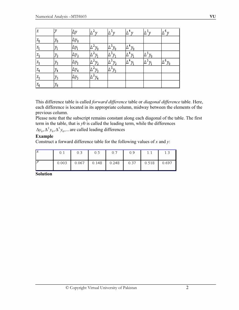
Numerical Analysis –MTH603 VU
© Copyright Virtual University of Pakistan 2
This difference table is called forward difference table or diagonal difference table. Here,
each difference is located in its appropriate column, midway between the elements of the
previous column.
Please note that the subscript remains constant along each diagonal of the table. The first
term in the table, that is y0 is called the leading term, while the differences 2 3
0 0 0, , ,...y y y! ! ! are called leading differences
Example
Construct a forward difference table for the following values of x and y:
Solution

Numerical Analysis –MTH603 VU
© Copyright Virtual University of Pakistan 3
Example
Express 2
0y! and 3
0y! in terms of the values of the function y.
Solution:
Noting that each higher order difference is defined in terms of the lower order difference,
we have
2
0 1 0 2 1 1 0
2 1 0
( ) ( )
2
y y y y y y y
y y y
! ! #! # # #
# "
And
3 2 2
0 1 0 2 1 1 0
3 2 2 1 2 1 1 0
3 2 1 0
( ) ( )
( ) ( ) ( ) ( )
3 3
yy y y y y y
y y y y y y y y
y y y y
! ! #! ! #! # ! #!
# # # # # " #
# " #
Hence, we observe that the coefficients of the values of y, in the expansion of 2 3
0 0,y y! ! , are binomial coefficients.
Thus, in general, we arrive at the following result: -
0 1 1 2 2 3 3 0( 1)n n n n n
n n n ny y C y C y C y y# # #! # " # " " #"
Example
Show that the value of yn can be expressed in terms of the leading value y0 and the
leading differences
2
0 0 0, , , .ny y y! ! !
SSoolluuttiioonn
TThhee ffoorrwwaarrdd ddiiffffeerreennccee ttaabbllee wwiillll bbee

Numerical Analysis –MTH603 VU
© Copyright Virtual University of Pakistan 4
1 0 0 1 0 0
2 1 1 2 1 1
3 2 2 3 2 2
or
or
or
y y y y y y
y y y y y y
y y y y y y
# ! " ! $%
# ! " ! &%# ! " ! '
Similarly,
2 2
1 0 0 1 0 0
2 2
2 1 1 2 1 1
or
or
y y y y y y
y y y y y y
$! #! ! ! ! " ! %&
! #! ! ! ! " ! %'
SSiimmiillaarrllyy,, wwee ccaann aallssoo wwrriittee
2 2 3 2 2 3
1 0 0 1 0 0
2 2 3 2 2 3
2 1 1 2 1 1
or
or
y y y y y y
y y y y y y
$! #! ! ! ! " ! %&
! #! ! ! ! " ! %'
2 2 3
2 0 0 0 0( ) ( )y y y y y! ! " ! " ! " !
2 3
0 0 02y y y ! " ! " !
2
3 2 2 1 1 1 1
2 3
0 0 0 0
( ) ( )
3 3
y y y y y y y
y y y y
" ! " ! " ! " !
" ! " ! " !
3
0(1 ) y " !
SSiimmiillaarrllyy,, wwee ccaann ssyymmbboolliiccaallllyy wwrriittee
1 0
2
2 0
3
3 0
0
(1 ) ,
(1 ) ,
(1 )
........
(1 )n
n
y y
y y
y y
y y
" !
" !
" !
" !
HHeennccee,, wwee oobbttaaiinn
2 3
0 1 0 2 0 3 0 0
n n n n
ny y C y C y C y y " ! " ! " ! " " !"
OR
0
0
nn i
n i
i
y C y
!(

Numerical Analysis –MTH603 VU
© Copyright Virtual University of Pakistan 1
BBaacckkwwaarrdd DDiiffffeerreenncceess FFoorr aa ggiivveenn ttaabbllee ooff vvaalluueess ( , ), 0,1, 2,...,k kx y k n ooff aa ffuunnccttiioonn yy == ff ((xx)) wwiitthh eeqquuaallllyy
ssppaacceedd aabbsscciissssaass,, tthhee ffiirrsstt bbaacckkwwaarrdd ddiiffffeerreenncceess aarree uussuuaallllyy eexxpprreesssseedd iinn tteerrmmss ooff tthhee
bbaacckkwwaarrdd ddiiffffeerreennccee ooppeerraattoorr ! aass
1 , ( 1), ,1i i iy y y i n n"! " "
TToo bbee eexxpplliicciitt,, wwee wwrriittee
OR
1 1 0
2 2 1
1n n n
y y y
y y y
y y y "
! "
! "
! "
! ! !
The differences of these differences are called second differences and they are denoted by 2 2 2
2 3, , , .ny y y! ! !
That is
2
1 2 1
2
2 3 2
2
1n n n
y y y
y y y
y y y "
! ! "!
! ! "!
! ! "!
! ! !
TThhuuss,, iinn ggeenneerraall,, tthhee sseeccoonndd bbaacckkwwaarrdd ddiiffffeerreenncceess aarree
2
1, , ( 1),..., 2i i iy y y i n n"! ! "! "
WWhhiillee tthhee kk--tthh bbaacckkwwaarrdd ddiiffffeerreenncceess aarree ggiivveenn aass
1 1
1, , ( 1),...,k k k
i i iy y y i n n k" ""! ! "! "
TThheessee bbaacckkwwaarrdd ddiiffffeerreenncceess ccaann bbee ssyysstteemmaattiiccaallllyy aarrrraannggeedd ffoorr aa ttaabbllee ooff vvaalluueess
( , ), 0,1,...,6k kx y k shown below.
BBaacckkwwaarrdd DDiiffffeerreennccee TTaabbllee

Numerical Analysis –MTH603 VU
© Copyright Virtual University of Pakistan 2
FFrroomm tthhiiss ttaabbllee,, iitt ccaann bbee oobbsseerrvveedd tthhaatt tthhee ssuubbssccrriipptt rreemmaaiinnss ccoonnssttaanntt aalloonngg eevveerryy
bbaacckkwwaarrdd ddiiaaggoonnaall..
EExxaammppllee SShhooww tthhaatt aannyy vvaalluuee ooff yy ccaann bbee eexxpprreesssseedd iinn tteerrmmss ooff yy
nn aanndd iittss bbaacckkwwaarrdd ddiiffffeerreenncceess..
SSoolluuttiioonn:: FFrroomm
1 , ( 1), ,1i i iy y y i n n"! " "
We get
1n n ny y y" "! 2 1 1n n ny y y" " " "!
From 2
1, , ( 1),..., 2i i iy y y i n n"! ! "! "
We get 2
1n n ny y y"! ! "!
FFrroomm tthheessee eeqquuaattiioonnss,, wwee oobbttaaiinn
2
2 2n n n ny y y y" " ! #!
SSiimmiillaarrllyy,, wwee ccaann sshhooww tthhaatt
2 3
3 3 3n n n n ny y y y y" " ! # ! "!
SSyymmbboolliiccaallllyy,, tthheessee rreessuullttss ccaann bbee rreewwrriitttteenn aass ffoolllloowwss::
1
2
2
3
3
(1 )
(1 )
(1 )
.......
(1 )
n n
n n
n n
r
n r n
y y
y y
y y
y y
"
"
"
"
"!
"!
"!
"!
2
1 2 ( 1)n n r r
n r n n n ny y C y C y y" " ! # ! " # " !"
CCeennttrraall DDiiffffeerreenncceess IInn ssoommee aapppplliiccaattiioonnss,, cceennttrraall ddiiffffeerreennccee nnoottaattiioonn iiss ffoouunndd ttoo bbee mmoorree ccoonnvveenniieenntt ttoo
rreepprreesseenntt tthhee ssuucccceessssiivvee ddiiffffeerreenncceess ooff aa ffuunnccttiioonn.. HHeerree,, wwee uussee tthhee ssyymmbbooll $ ttoo
rreepprreesseenntt cceennttrraall ddiiffffeerreennccee ooppeerraattoorr aanndd tthhee ssuubbssccrriipptt ooff y$ bbbb ffoorr aannyy ddiiffffeerreennccee aass
tthhee aavveerraaggee ooff tthhee ssuubbssccrriippttss
1 2 1 0 3 2 2 1, ,y y y y y y$ $ " "
In General,
(1 2) (1 2)i i iy y y$ # " "

Numerical Analysis –MTH603 VU
© Copyright Virtual University of Pakistan 3
HHiigghheerr oorrddeerr ddiiffffeerreenncceess aarree ddeeffiinneedd aass ffoolllloowwss::
2
(1 2) (1 2)i i iy y y$ $ $# " "
1 1
(1 2) (1 2)
n n n
i i iy y y$ $ $" "# " "
TThheessee cceennttrraall ddiiffffeerreenncceess ccaann bbee ssyysstteemmaattiiccaallllyy aarrrraannggeedd aass iinnddiiccaatteedd iinn tthhee TTaabbllee
TThhuuss,, wwee oobbsseerrvvee tthhaatt aallll tthhee oodddd ddiiffffeerreenncceess hhaavvee aa ffrraaccttiioonnaall ssuuffffiixx aanndd aallll tthhee eevveenn
ddiiffffeerreenncceess wwiitthh tthhee ssaammee ssuubbssccrriipptt lliiee hhoorriizzoonnttaallllyy..
TThhee ffoolllloowwiinngg aalltteerrnnaattiivvee nnoottaattiioonn mmaayy aallssoo bbee aaddoopptteedd ttoo iinnttrroodduuccee ffiinniittee ddiiffffeerreennccee
ooppeerraattoorrss.. LLeett yy == ff ((xx)) bbee aa ffuunnccttiioonnaall rreellaattiioonn bbeettwweeeenn xx aanndd yy,, wwhhiicchh iiss aallssoo ddeennootteedd bbyy
yyxx..
SSuuppppoossee,, wwee aarree ggiivveenn ccoonnsseeccuuttiivvee vvaalluueess ooff xx ddiiffffeerriinngg bbyy hh ssaayy xx,, xx ++ hh,, xx ++22hh,, xx ++33hh,,
eettcc.. TThhee ccoorrrreessppoonnddiinngg vvaalluueess ooff yy aarree 2 3, , , ,x x h x h x hy y y y# # #
AAss bbeeffoorree,, wwee ccaann ffoorrmm tthhee ddiiffffeerreenncceess ooff tthheessee vvaalluueess..
Thus
( ) ( )x x h xy y y f x h f x#% " # "
2
x x h xy y y#% % "%
Similarly,
( ) ( )x x x hy y y f x f x h"! " " "
( / 2) ( / 2)2 2
x x h x h
h hy y y f x f x$ # "
& ' & ' " # " "( ) ( )
* + * +
TToo bbee eexxpplliicciitt,, wwee wwrriittee
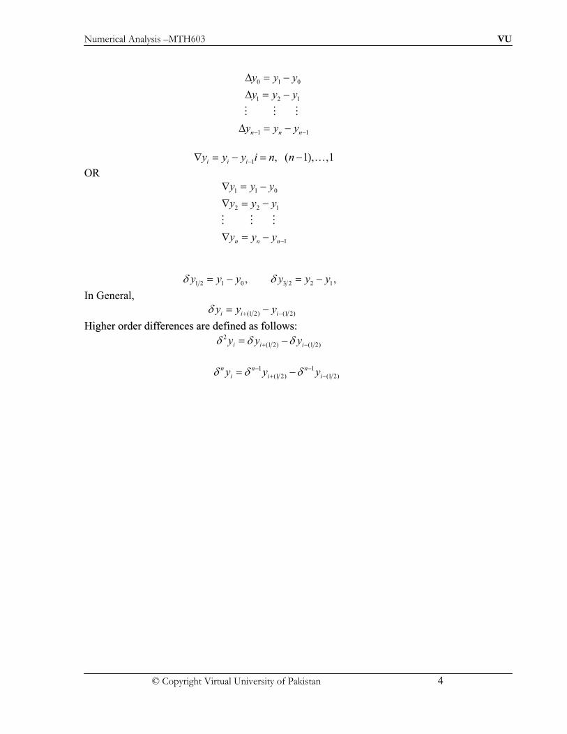
Numerical Analysis –MTH603 VU
© Copyright Virtual University of Pakistan 4
0 1 0
1 2 1
1 1n n n
y y y
y y y
y y y" "
% "
% "
% "
! ! !
1 , ( 1), ,1i i iy y y i n n"! " "
OR
1 1 0
2 2 1
1n n n
y y y
y y y
y y y "
! "
! "
! "
! ! !
1 2 1 0 3 2 2 1, ,y y y y y y$ $ " "
In General,
(1 2) (1 2)i i iy y y$ # " "
HHiigghheerr oorrddeerr ddiiffffeerreenncceess aarree ddeeffiinneedd aass ffoolllloowwss::
2
(1 2) (1 2)i i iy y y$ $ $# " "
1 1
(1 2) (1 2)
n n n
i i iy y y$ $ $" "# " "

Numerical Analysis –MTH603 VU
© Copyright Virtual University of Pakistan 1
SShhiifftt ooppeerraattoorr,, EE LLeett yy == ff ((xx)) bbee aa ffuunnccttiioonn ooff xx,, aanndd lleett xx ttaakkeess tthhee ccoonnsseeccuuttiivvee vvaalluueess xx,, xx ++ hh,, xx ++ 22hh,, eettcc..
WWee tthheenn ddeeffiinnee aann ooppeerraattoorr hhaavviinngg tthhee pprrooppeerrttyy
( ) ( )E f x f x h !
TThhuuss,, wwhheenn EE ooppeerraatteess oonn ff ((xx)),, tthhee rreessuulltt iiss tthhee nneexxtt vvaalluuee ooff tthhee ffuunnccttiioonn.. HHeerree,, EE iiss
ccaalllleedd tthhee sshhiifftt ooppeerraattoorr.. IIff wwee aappppllyy tthhee ooppeerraattoorr EE ttwwiiccee oonn ff ((xx)),, wwee ggeett
2 ( ) [ ( )]
[ ( )] ( 2 )
E f x E E f x
E f x h f x h
! !
TThhuuss,, iinn ggeenneerraall,, iiff wwee aappppllyy tthhee ooppeerraattoorr ‘‘EE’’ nn ttiimmeess oonn ff ((xx)),, wwee ggeett
( ) ( )nE f x f x nh !
OR
n
x x nhE y y !
2 4 2
0 1 0 2 0 4 2 4, , , ,Ey y E y y E y y E y y
TThhee iinnvveerrssee ooppeerraattoorr EE--11
iiss ddeeffiinneedd aass
1 ( ) ( )E f x f x h" "
SSiimmiillaarrllyy
( ) ( )nE f x f x nh" "
AAvveerraaggee OOppeerraattoorr,, # ;;
iitt iiss ddeeffiinneedd aass
( / 2) ( / 2)
1( )
2 2 2
1
2x h x h
h hf x f x f x
y y
#
! "
$ %& ' & ' ! ! "( ) ( )* +, - , -. /
$ % !. /
DDiiffffeerreennttiiaall OOppeerraattoorr,, DD iitt iiss ddeeffiinneedd aass
2
2
2
( ) ( ) ( )
( ) ( ) ( )
dDf x f x f x
dx
dD f x f x f x
dx
01 223211 24
IImmppoorrttaanntt RReessuullttss UUssiinngg {{ , , , ,E5 #6 7 }}
( 1)
x x h x x x
x
y y y Ey y
E y
!6 " "
"
1E86 " Also
1
1(1 )
x x x h x x
x
y y y y E y
E y
""
"
7 " "
"

Numerical Analysis –MTH603 VU
© Copyright Virtual University of Pakistan 2
1 11
EE
E
" "87 "
And
( / 2) ( / 2)
1/ 2 1/ 2
1/ 2 1/ 2( )
x x h x h
x x
x
y y y
E y E y
E E y
5 ! "
"
"
"
"
"
1/ 2 1/ 2E E5 " " TThhee ddeeffiinniittiioonn ooff # aanndd EE ssiimmiillaarrllyy yyiieellddss
( / 2) ( / 2)
1/ 2 1/ 2
1
2
1( )
2
x x h x h
x
y y y
E E y
# ! "
"
$ % !. /
!
1/ 2 1/ 21( )
2E E# "8 !
We know that
( )x x hEy y f x h! !
2
( ) ( ) ( )2!
x
hEy f x hf x f x1 11 ! ! !!
2
2( ) ( ) ( )2!
hf x hDf x D f x ! ! !!
2 2
1 ( )1! 2!
hD
x
hD h Df x e y
& ' ! ! ! ( ), -
!
Thus
loghD E
EExxaammppllee:: PPrroovvee tthhaatt
1
log(1 )
log(1 )
sinh ( )
hD
#5"
! 6
" "7
SSoolluuttiioonn:: UUssiinngg tthhee ssttaannddaarrdd rreellaattiioonnss wwee hhaavvee
1
log
log(1 )
log
log(1 )
hD E
E"
! 6
"
" "7

Numerical Analysis –MTH603 VU
© Copyright Virtual University of Pakistan 3
1/ 2 1/ 2 1/ 2 1/ 2
1
1
1( )( )
2
1( )
2
1( )
2
sinh( )
sinh
hD hD
E E E E
E E
e e
hD
hD
#5
#5
" "
"
"
"
! "
"
"
8
Example Prove that
1)
22
2 21 12
55 #
& '! !( )
, -
2) 1/ 2
2E
5# !
3) 2
21 ( / 4)2
55 56 ! !
4) 1
2 2
E#5
"6 6 !
5) 2
!" #$
%
SSoolluuttiioonn FFrroomm tthhee ddeeffiinniittiioonn,, wwee hhaavvee::
(1) 1/ 2 1/ 2 1/ 2 1/ 2 11 1( )( ) ( )
2 2E E E E E E ! & & &% # & % &
2 2 2 2 1 21 11 1 ( 2 ) ( )
4 4E E E E ! & &' # % # & # % #
2
1/ 2 1/ 2 2 1 21 11 1 ( ) ( )
2 2 2E E E E
! & &# % # & % #
(2)
1/ 2 1/ 2 1/ 2 1/ 2 1/ 2
( / 2)
1( )
2E E E E E
!
& &
#
% # # & %
((33))

Numerical Analysis –MTH603 VU
© Copyright Virtual University of Pakistan 4
( ) ( ) ( )21/ 2 1/ 2 1/ 2 1/ 22
1/ 2 1/ 222
11
41 ( / 4)2 2 1
E E E EE E!! !
& && & # &&
# # % #
1
1/ 2 1/ 2 1/ 2 1/ 22 1( )( )
2 2
E EE E E E
&& && #
% # & #
1 12
2 2
E E E E& && # &% #
1E% & % " (4)
1/ 2 1/ 2 1/ 2 1/ 2 11 1( )( ) ( )
2 2E E E E E E ! & & &% # & % &
1 11 1(1 ) (1 )
2 2 2E E& &"
% # " & % # &
1 1
2 2 2 2
E
E E
" & " "* +% # % #, -. /
(5)
1/ 2 1/ 2 1/ 2 1/ 2
1
1( )( )
2
1( )
2
E E E E
E E
! & &
&
% # &
% &
1 1
(1 1 ) ( )2 2
% # " & #$ % " #$

Numerical Analysis –MTH603 VU
© Copyright Virtual University of Pakistan 1
Interpolation Newton’s Forward Difference Formula LLeett yy == ff ((xx)) bbee aa ffuunnccttiioonn wwhhiicchh ttaakkeess vvaalluueess ff((xx
00)),, ff((xx
00++ hh)),, ff((xx
00++22hh)),, ……,, ccoorrrreessppoonnddiinngg
ttoo vvaarriioouuss eeqquuii--ssppaacceedd vvaalluueess ooff xx wwiitthh ssppaacciinngg hh,, ssaayy xx00
,, xx00 ++ hh,, xx
00 ++ 22hh,, …… ..
SSuuppppoossee,, wwee wwiisshh ttoo eevvaalluuaattee tthhee ffuunnccttiioonn ff ((xx)) ffoorr aa vvaalluuee xx00
++ pphh,, wwhheerree pp iiss aannyy rreeaall
nnuummbbeerr,, tthheenn ffoorr aannyy rreeaall nnuummbbeerr pp,, wwee hhaavvee tthhee ooppeerraattoorr EE ssuucchh tthhaatt
( ) ( ).pE f x f x ph !
0 0 0( ) ( ) (1 ) ( )p pf x ph E f x f x! ! "
2 3
0
( 1) ( 1)( 2)1 ( )
2! 3!
p p p p pp f x
# # #$ % ! " ! " ! " !& '( )
0 0 0
2 3
0 0
0
( ) ( ) ( )
( 1) ( 1)( 2)( ) ( )
2! 3!
( 1) ( 1)( ) Error
!
n
f x ph f x p f x
p p p p pf x f x
p p p nf x
n
! ! "
# # #! " ! "
# # !! ! " !
TThhiiss iiss kknnoowwnn aass NNeewwttoonn’’ss ffoorrwwaarrdd ddiiffffeerreennccee ffoorrmmuullaa ffoorr iinntteerrppoollaattiioonn,, wwhhiicchh ggiivveess tthhee
vvaalluuee ooff ff((xx00 ++ pphh)) iinn tteerrmmss ooff ff((xx
00)) aanndd iittss lleeaaddiinngg ddiiffffeerreenncceess..
TThhiiss ffoorrmmuullaa iiss aallssoo kknnoowwnn aass NNeewwttoonn--GGrreeggoorryy ffoorrwwaarrdd ddiiffffeerreennccee iinntteerrppoollaattiioonn ffoorrmmuullaa..
HHeerree pp==((xx--xx00))//hh..
AAnn aalltteerrnnaattee eexxpprreessssiioonn iiss
2 3
0 0 0 0
0
( 1) ( 1)( 2)
2! 3!
( 1)( 1)Error
!
x
n
p p p p py y p y y y
p p p ny
n
# # # ! " ! " ! " !
# # !! " !
IIff wwee rreettaaiinn ((rr ++ 11)) tteerrmmss,, wwee oobbttaaiinn aa ppoollyynnoommiiaall ooff ddeeggrreeee rr aaggrreeeeiinngg wwiitthh yyxx aatt
xx00,, xx11,, ……,, xxrr..
TThhiiss ffoorrmmuullaa iiss mmaaiinnllyy uusseedd ffoorr iinntteerrppoollaattiinngg tthhee vvaalluueess ooff yy nneeaarr tthhee bbeeggiinnnniinngg ooff aa sseett ooff
ttaabbuullaarr vvaalluueess aanndd ffoorr eexxttrraappoollaattiinngg vvaalluueess ooff yy,, aa sshhoorrtt ddiissttaannccee bbaacckkwwaarrdd ffrroomm yy00
EExxaammppllee:: EEvvaalluuaattee ff ((1155)),, ggiivveenn tthhee ffoolllloowwiinngg ttaabbllee ooff vvaalluueess::
SSoolluuttiioonn::
TThhee ffoorrwwaarrdd ddiiffffeerreenncceess aarree ttaabbuullaatteedd aass
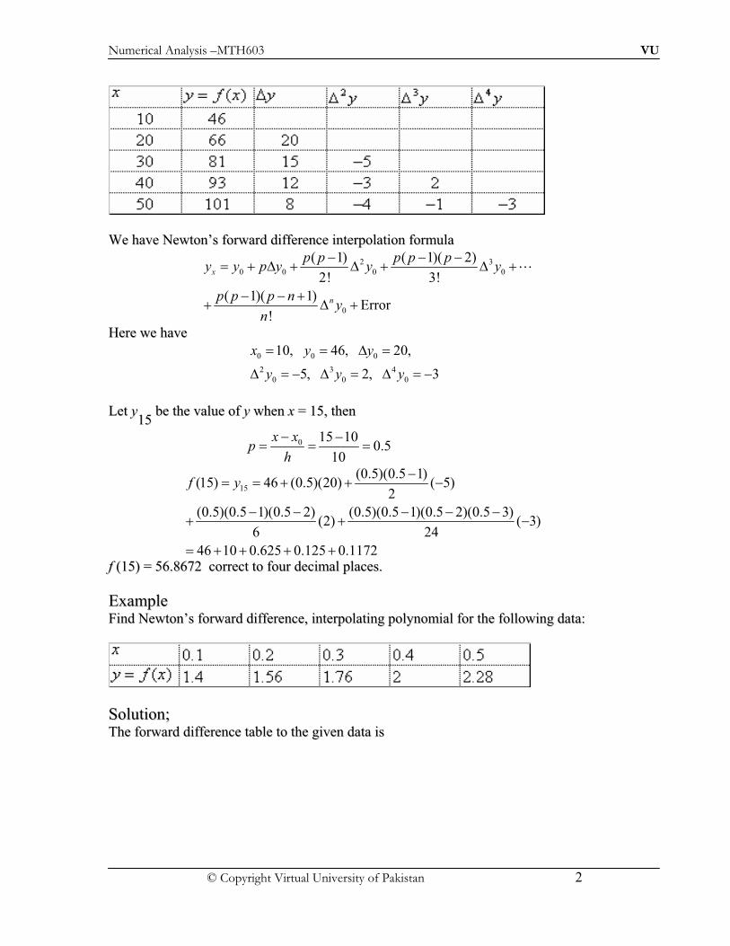
Numerical Analysis –MTH603 VU
© Copyright Virtual University of Pakistan 2
WWee hhaavvee NNeewwttoonn’’ss ffoorrwwaarrdd ddiiffffeerreennccee iinntteerrppoollaattiioonn ffoorrmmuullaa
2 3
0 0 0 0
0
( 1) ( 1)( 2)
2! 3!
( 1)( 1)Error
!
x
n
p p p p py y p y y y
p p p ny
n
# # # ! " ! " ! " !
# # !! " !
HHeerree wwee hhaavvee
0 0 0
2 3 4
0 0 0
10, 46, 20,
5, 2, 3
x y y
y y y
"
" # " " #
LLeett yy1155
bbee tthhee vvaalluuee ooff yy wwhheenn xx == 1155,, tthheenn
0 15 100.5
10
x xp
h
# #
15
(0.5)(0.5 1)(15) 46 (0.5)(20) ( 5)
2
(0.5)(0.5 1)(0.5 2) (0.5)(0.5 1)(0.5 2)(0.5 3)(2) ( 3)
6 24
46 10 0.625 0.125 0.1172
f y#
! ! #
# # # # #! ! #
! ! ! !
ff ((1155)) == 5566..88667722 ccoorrrreecctt ttoo ffoouurr ddeecciimmaall ppllaacceess..
EExxaammppllee FFiinndd NNeewwttoonn’’ss ffoorrwwaarrdd ddiiffffeerreennccee,, iinntteerrppoollaattiinngg ppoollyynnoommiiaall ffoorr tthhee ffoolllloowwiinngg ddaattaa::
SSoolluuttiioonn;; TThhee ffoorrwwaarrdd ddiiffffeerreennccee ttaabbllee ttoo tthhee ggiivveenn ddaattaa iiss

Numerical Analysis –MTH603 VU
© Copyright Virtual University of Pakistan 3
SSiinnccee,, 33rrdd
aanndd 44tthh
lleeaaddiinngg ddiiffffeerreenncceess aarree zzeerroo,, wwee hhaavvee NNeewwttoonn’’ss ffoorrwwaarrdd ddiiffffeerreennccee
iinntteerrppoollaattiinngg ffoorrmmuullaa aass
2
0 0 0
( 1)
2
p py y p y y
# ! " ! "
In this problem,
0 0
2
0 0
0.1, 1.40,
0.16, 0.04,
x y
y y
" "
and
0.1
10 10.1
xp x
# #
SSuubbssttiittuuttiinngg tthheessee vvaalluueess,,
(10 1)(10 2)
( ) 1.40 (10 1)(0.16) (0.04)2
x xy f x x
# # ! # !
TThhiiss iiss tthhee rreeqquuiirreedd NNeewwttoonn’’ss iinntteerrppoollaattiinngg ppoollyynnoommiiaall..
EExxaammppllee EEssttiimmaattee tthhee mmiissssiinngg ffiigguurree iinn tthhee ffoolllloowwiinngg ttaabbllee::
SSoolluuttiioonn
SSiinnccee wwee aarree ggiivveenn ffoouurr eennttrriieess iinn tthhee ttaabbllee,, tthhee ffuunnccttiioonn yy == ff ((xx)) ccaann bbee rreepprreesseenntteedd bbyy aa
ppoollyynnoommiiaall ooff ddeeggrreeee tthhrreeee..
3
4
( ) Constant
and ( ) 0,
f x
f x x
"
" *
In particular,
4
0( ) 0f x"
EEqquuiivvaalleennttllyy,,
4
0( 1) ( ) 0E f x#

Numerical Analysis –MTH603 VU
© Copyright Virtual University of Pakistan 4
EExxppaannddiinngg,, wwee hhaavvee
4 3 2
0( 4 6 4 1) ( ) 0E E E E f x# ! # !
TThhaatt iiss,,
4 3 2 1 0( ) 4 ( ) 6 ( ) 4 ( ) ( ) 0f x f x f x f x f x# ! # !
UUssiinngg tthhee vvaalluueess ggiivveenn iinn tthhee ttaabbllee,, wwee oobbttaaiinn
332 4 ( ) 6 7 4 5 2 0f x# ! + # + !
wwhhiicchh ggiivveess ff ((xx33)),, tthhee mmiissssiinngg vvaalluuee eeqquuaall ttoo 1144..
EExxaammppllee
Consider the following table of values
x .2 .3 .4 .5 .6
F(x) .2304 .2788 .3222 .3617 .3979
Find f (.36) using Newton’s Forward Difference Formula.
Solution
x ( )y f x y" 2 y"
3 y" 4 y"
0.2 0.2304 0.0484 -0.005 0.0011 -0.0005
0.3 0.2788 0.0434 -0.0039 0.0006
0.4 0.3222 0.0395 -0.0033
0.5 0.3617 0.0362
0.6 0.3979
2 3
0 0 0 0
4
0 0
( 1) ( 1)( 2)
2! 3!
( 1)( 2)( 3) ( 1)( 2)........( 1)
4! !
x
n
p p p p py y p y y y
p p p p p p p p ny y
n
# # # ! " ! " ! "
# # # # # # !! " ! ! "
Where
0 0 0
2 3 4
0 0 0
0.2, 0.2304, 0.0484,
0.005, 0.0011, .0005
x y y
y y y
"
" # " " #0 0.36 0.2
1.60.1
x xp
h
# #
, -1.6(1.6 1) 1.6(1.6 1)(1.6 2) 1.6(1.6 1)(1.6 2)(1.6 3)0.2304 1.6(0.0484) 0.005 (0.0011) ( .0005)
2! 3! 4!
1.6(.6)( .4) 1.6(.6)( .4)( 1.4)0.2304 .077441 .0024 (.0011) ( .0005)
6 24
0.3078 .0024 .00007 .0000
xy# # # # # #
! ! # ! ! #
# # # ! # ! ! #
# # # 1
.3053

Numerical Analysis –MTH603 VU
© Copyright Virtual University of Pakistan 5
EExxaammppllee FFiinndd aa ccuubbiicc ppoollyynnoommiiaall iinn xx wwhhiicchh ttaakkeess oonn tthhee vvaalluueess
--33,, 33,, 1111,, 2277,, 5577 aanndd 110077,, wwhheenn xx == 00,, 11,, 22,, 33,, 44 aanndd 55 rreessppeeccttiivveellyy..
SSoolluuttiioonn HHeerree,, tthhee oobbsseerrvvaattiioonnss aarree ggiivveenn aatt eeqquuaall iinntteerrvvaallss ooff uunniitt wwiiddtthh..
TToo ddeetteerrmmiinnee tthhee rreeqquuiirreedd ppoollyynnoommiiaall,, wwee ffiirrsstt ccoonnssttrruucctt tthhee ddiiffffeerreennccee ttaabbllee
DDiiffffeerreennccee TTaabbllee
SSiinnccee tthhee 44tthh
aanndd hhiigghheerr oorrddeerr ddiiffffeerreenncceess aarree zzeerroo,, tthhee rreeqquuiirreedd NNeewwttoonn’’ss iinntteerrppoollaattiioonn
ffoorrmmuullaa
2 3
0 0 0 0 0
( 1) ( 1)( 2)( ) ( ) ( ) ( ) ( )
2 6
p p p p pf x ph f x p f x f x f x
# # #! ! " ! " ! "
Here
0
0
2
0
3
0
0
1
( ) 6
( ) 2
( ) 6
x x xp x
h
f x
f x
f x
# #
"
"
"
SSuubbssttiittuuttiinngg tthheessee vvaalluueess iinnttoo tthhee ffoorrmmuullaa,, wwee hhaavvee
( 1) ( 1)( 2)
( ) 3 6 (2) (6)2 6
x x x x xf x x
# # # # ! ! !
3 2( ) 2 7 3,f x x x x # ! #
TThhee rreeqquuiirreedd ccuubbiicc ppoollyynnoommiiaall..

Numerical Analysis –MTH603 VU
© Copyright Virtual University of Pakistan 1
NNEEWWTTOONN’’SS BBAACCKKWWAARRDD DDIIFFFFEERREENNCCEE IINNTTEERRPPOOLLAATTIIOONN
FFOORRMMUULLAA FFoorr iinntteerrppoollaattiinngg tthhee vvaalluuee ooff tthhee ffuunnccttiioonn yy == ff ((xx)) nneeaarr tthhee eenndd ooff ttaabbllee ooff vvaalluueess,, aanndd ttoo
eexxttrraappoollaattee vvaalluuee ooff tthhee ffuunnccttiioonn aa sshhoorrtt ddiissttaannccee ffoorrwwaarrdd ffrroomm yynn,, NNeewwttoonn’’ss bbaacckkwwaarrdd
iinntteerrppoollaattiioonn ffoorrmmuullaa iiss uusseedd
DDeerriivvaattiioonn LLeett yy == ff ((xx)) bbee aa ffuunnccttiioonn wwhhiicchh ttaakkeess oonn vvaalluueess
ff ((xxnn)),, ff ((xx
nn--hh)),, ff ((xx
nn--22hh)),, ……,, ff ((xx
00)) ccoorrrreessppoonnddiinngg ttoo eeqquuiissppaacceedd vvaalluueess xx
nn,, xx
nn--hh,, xx
nn--22hh,,
……,, xx00.. SSuuppppoossee,, wwee wwiisshh ttoo eevvaalluuaattee tthhee ffuunnccttiioonn ff ((xx)) aatt ((xx
nn ++ pphh)),, wwhheerree pp iiss aannyy rreeaall
nnuummbbeerr,, tthheenn wwee hhaavvee tthhee sshhiifftt ooppeerraattoorr EE,, ssuucchh tthhaatt 1( ) ( ) ( ) ( ) (1 ) ( )p p p
n n n nf x ph E f x E f x f x ! " " " #
BBiinnoommiiaall eexxppaannssiioonn yyiieellddss,,
2 3( 1) ( 1)( 2)( ) 1
2! 3!
( 1)( 2) ( 1)Error ( )
!
n
n
n
p p p p pf x ph p
p p p p nf x
n
! ! !$! " ! # ! # ! # !%&! ! ! '! # ! ()
That is
2 3( 1) ( 1)( 2)( ) ( ) ( ) ( ) ( )
2! 3!
( 1)( 2) ( 1)( ) Error
!
n n n n n
n
n
p p p p pf x ph f x p f x f x f x
p p p p nf x
n
! ! !! " ! # ! # ! # !
! ! ! ! # !
TThhiiss ffoorrmmuullaa iiss kknnoowwnn aass NNeewwttoonn’’ss bbaacckkwwaarrdd iinntteerrppoollaattiioonn ffoorrmmuullaa.. TThhiiss ffoorrmmuullaa iiss aallssoo
kknnoowwnn aass NNeewwttoonn’’ss--GGrreeggoorryy bbaacckkwwaarrdd ddiiffffeerreennccee iinntteerrppoollaattiioonn ffoorrmmuullaa..
IIff wwee rreettaaiinn ((rr ++ 11))tteerrmmss,, wwee oobbttaaiinn aa ppoollyynnoommiiaall ooff ddeeggrreeee rr aaggrreeeeiinngg wwiitthh ff ((xx)) aatt xxnn,,
xxnn--11
,, ……,, xxnn--rr
.. AAlltteerrnnaattiivveellyy,, tthhiiss ffoorrmmuullaa ccaann aallssoo bbee wwrriitttteenn aass
2 3( 1) ( 1)( 2)
2! 3!
( 1)( 2) ( 1)Error
!
x n n n n
n
n
p p p p py y p y y y
p p p p ny
n
! ! !" ! # ! # ! # !
! ! ! ! # !
Here nx xp
h
"
EExxaammppllee FFoorr tthhee ffoolllloowwiinngg ttaabbllee ooff vvaalluueess,, eessttiimmaattee ff ((77..55))..

Numerical Analysis –MTH603 VU
© Copyright Virtual University of Pakistan 2
SSoolluuttiioonn
TThhee vvaalluuee ttoo bbee iinntteerrppoollaatteedd iiss aatt tthhee eenndd ooff tthhee ttaabbllee.. HHeennccee,, iitt iiss aapppprroopprriiaattee ttoo uussee
NNeewwttoonn’’ss bbaacckkwwaarrdd iinntteerrppoollaattiioonn ffoorrmmuullaa.. LLeett uuss ffiirrsstt ccoonnssttrruucctt tthhee bbaacckkwwaarrdd ddiiffffeerreennccee
ttaabbllee ffoorr tthhee ggiivveenn ddaattaa
DDiiffffeerreennccee TTaabbllee
SSiinnccee tthhee 44tthh
aanndd hhiigghheerr oorrddeerr ddiiffffeerreenncceess aarree zzeerroo,, tthhee rreeqquuiirreedd NNeewwttoonn’’ss bbaacckkwwaarrdd
iinntteerrppoollaattiioonn ffoorrmmuullaa iiss
2
3
( 1)
2!
( 1)( 2)
3!
x n n n
n
p py y p y y
p p py
!" ! # ! #
! !! #
IInn tthhiiss pprroobblleemm,,
7.5 8.0
0.51
nx xp
h
" " "
2 3169, 42, 6n n ny y y# " # " # "
7.5
( 0.5)(0.5)512 ( 0.5)(169) (42)
2
( 0.5)(0.5)(1.5)(6)
6
512 84.5 5.25 0.375
421.875
y
" ! !
!
"
"
EExxaammppllee TThhee ssaalleess ffoorr tthhee llaasstt ffiivvee yyeeaarrss iiss ggiivveenn iinn tthhee ttaabbllee bbeellooww.. EEssttiimmaattee tthhee ssaalleess ffoorr tthhee yyeeaarr
11997799

Numerical Analysis –MTH603 VU
© Copyright Virtual University of Pakistan 3
SSoolluuttiioonn
NNeewwttoonn’’ss bbaacckkwwaarrdd ddiiffffeerreennccee TTaabbllee
In this example,
1979 1982
1.52
p
" "
and
2
3 4
5, 1,
2, 5
n n
n n
y y
y y
# " # "
# " # "
NNeewwttoonn’’ss iinntteerrppoollaattiioonn ffoorrmmuullaa ggiivveess
1979
( 1.5)( 0.5) ( 1.5)( 0.5)(0.5)57 ( 1.5)5 (1) (2)
2 6
( 1.5)( 0.5)(0.5)(1.5)(5)
24
y
" ! ! !
!
57 7.5 0.375 0.125 0.1172" ! ! !
Therefore,
1979 50.1172y "
Example
Consider the following table of values
x 1 1.1 1.2 1.3 1.4 1.5
F(x) 2 2.1 2.3 2.7 3.5 4.5
Use Newton’s Backward Difference Formula to estimate the value of f(1.45) .
Solution
x y=F(x) y# 2 y#
3 y# 4 y#
5 y#
1 2
1.1 2.1 0.1
1.2 2.3 0.2 0.1
1.3 2.7 0.4 0.2 0.1
1.4 3.5 0.8 0.4 0.2 0.1
1.5 4.5 1 0.2 -0.2 -0.4 -0.5

Numerical Analysis –MTH603 VU
© Copyright Virtual University of Pakistan 4
1.45 1.50.5
0.1
nx xp
h
" " " , ny# = 1 , 2
ny# = .2 , 3
ny# = - .2 , 4
ny# = -.4 ,
5
ny# = -.5
As we know that
2 3
4 5
( 1) ( 1)( 2)
2! 3!
( 1)( 2)( 3) ( 1)( 2)( 3)( 4)
4! 5!
x n n n n
n n
p p p p py y p y y y
p p p p p p p p py y
! ! !" ! # ! # ! #
! ! ! ! ! ! !! # ! #
* + * + * + * +
* + * + * + * +
0.5 ( 0.5 1) 0.5 ( 0.5 1)( 0.5 2)4.5 0.5 (1) (0.2) 0.2
2! 3!
0.5 ( 0.5 1)( 0.5 2)( 0.5 3) 0.5 ( 0.5 1)( 0.5 2)( 0.5 3)( 0.5 4)0.4 0.5
4! 5!
xy ! ! !
" ! ! !
! ! ! ! ! ! !! !
= 4.5 0.5 0.025 + 0.0125 + 0.015625+ 0.068359
4.07148
"

Numerical Analysis –MTH603 VU
© Copyright Virtual University of Pakistan 1
LLAAGGRRAANNGGEE’’SS IINNTTEERRPPOOLLAATTIIOONN FFOORRMMUULLAA NNeewwttoonn’’ss iinntteerrppoollaattiioonn ffoorrmmuullaaee ddeevveellooppeedd eeaarrlliieerr ccaann bbee uusseedd oonnllyy wwhheenn tthhee vvaalluueess ooff
tthhee iinnddeeppeennddeenntt vvaarriiaabbllee xx aarree eeqquuaallllyy ssppaacceedd.. AAllssoo tthhee ddiiffffeerreenncceess ooff yy mmuusstt uullttiimmaatteellyy
bbeeccoommee ssmmaallll..
IIff tthhee vvaalluueess ooff tthhee iinnddeeppeennddeenntt vvaarriiaabbllee aarree nnoott ggiivveenn aatt eeqquuiiddiissttaanntt iinntteerrvvaallss,, tthheenn wwee
hhaavvee tthhee bbaassiicc ffoorrmmuullaa aassssoocciiaatteedd wwiitthh tthhee nnaammee ooff LLaaggrraannggee wwhhiicchh wwiillll bbee ddeerriivveedd nnooww..
LLeett yy == ff ((xx)) bbee aa ffuunnccttiioonn wwhhiicchh ttaakkeess tthhee vvaalluueess,, yy00
,, yy11
,,……yynn ccoorrrreessppoonnddiinngg ttoo xx
00
,, xx11,, ……xx
nn .. SSiinnccee tthheerree aarree ((nn ++ 11)) vvaalluueess ooff yy ccoorrrreessppoonnddiinngg ttoo ((nn ++ 11)) vvaalluueess ooff xx,, wwee
ccaann rreepprreesseenntt tthhee ffuunnccttiioonn ff ((xx)) bbyy aa ppoollyynnoommiiaall ooff ddeeggrreeee nn..
SSuuppppoossee wwee wwrriittee tthhiiss ppoollyynnoommiiaall iinn tthhee ffoorrmm ..
1
0 1( ) n n
nf x A x A x A ! " " "
or in the form,
0 1 2
1 0 2
2 0 1
0 1 1
( ) ( )( ) ( )
( )( ) ( )
( )( ) ( )
( )( ) ( )
n
n
n
n n
y f x a x x x x x x
a x x x x x x
a x x x x x x
a x x x x x x
! !
"
" "
"
HHeerree,, tthhee ccooeeffffiicciieennttss aakk aarree ssoo cchhoosseenn aass ttoo ssaattiissffyy tthhiiss eeqquuaattiioonn bbyy tthhee ((nn ++ 11)) ppaaiirrss
((xxii,, yy
ii)).. TThhuuss wwee ggeett
0 0 0 0 1 0 1 0 2 0( ) ( )( )( ) ( )ny f x a x x x x x x x x! !
Therefore,
00
0 1 0 2 0( )( ) ( )n
ya
x x x x x x!
Similarily,we obtain
11
1 0 1 2 1( )( ) ( )n
ya
x x x x x x!
and
0 1 1 1( )( ) ( )( ) ( )
ii
i i i i i i i n
ya
x x x x x x x x x x "
!
0 1 1( )( ) ( )
nn
n n n n
ya
x x x x x x
!
SSuubbssttiittuuttiinngg tthhee vvaalluueess ooff aa00,, aa
11,, ……,, aa
nn wwee ggeett
1 2 0 20 1
0 1 0 2 0 1 0 1 2 1
( )( ) ( ) ( )( ) ( )( )
( )( ) ( ) ( )( ) ( )
n n
n n
x x x x x x x x x x x xy f x y y
x x x x x x x x x x x x
! ! " "
0 1 1 1
0 1 1 1
( )( ) ( )( ) ( )
( )( ) ( )( ) ( )
i i ni
i i i i i i i n
x x x x x x x x x xy
x x x x x x x x x x
"
"
" "
TThhee LLaaggrraannggee’’ss ffoorrmmuullaa ffoorr iinntteerrppoollaattiioonn
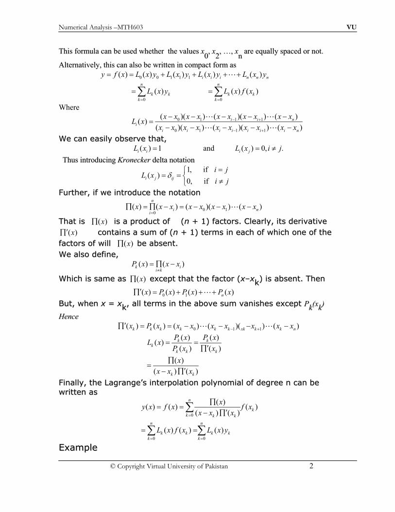
Numerical Analysis –MTH603 VU
© Copyright Virtual University of Pakistan 2
TThhiiss ffoorrmmuullaa ccaann bbee uusseedd wwhheetthheerr tthhee vvaalluueess xx00,, xx
22,, ……,, xx
nn aarree eeqquuaallllyy ssppaacceedd oorr nnoott..
AAlltteerrnnaattiivveellyy,, tthhiiss ccaann aallssoo bbee wwrriitttteenn iinn ccoommppaacctt ffoorrmm aass
0 0 1 1 1( ) ( ) ( ) ( ) ( )i i i n n ny f x L x y L x y L x y L x y! ! " " " "
0
( )n
k k
k
L x y!
!# 0
( ) ( )n
k k
k
L x f x!
!#
Where
0 1 1 1
0 1 1 1
( )( ) ( )( ) ( )( )
( )( ) ( )( ) ( )
i i ni
i i i i i i i n
x x x x x x x x x xL x
x x x x x x x x x x
"
"
!
WWee ccaann eeaassiillyy oobbsseerrvvee tthhaatt,, ( ) 1i iL x ! and ( ) 0, .i jL x i j! $
TThhuuss iinnttrroodduucciinngg KKrroonneecckkeerr ddeellttaa nnoottaattiioonn
1, if
( )0, if
i j ij
i jL x
i j%
!&! ! '
$(
FFuurrtthheerr,, iiff wwee iinnttrroodduuccee tthhee nnoottaattiioonn
0 10
( ) ( ) ( )( ) ( )n
i ni
x x x x x x x x x!
) !) !
TThhaatt iiss ( )x) iiss aa pprroodduucctt ooff ((nn ++ 11)) ffaaccttoorrss.. CClleeaarrllyy,, iittss ddeerriivvaattiivvee
( )x*) ccoonnttaaiinnss aa ssuumm ooff ((nn ++ 11)) tteerrmmss iinn eeaacchh ooff wwhhiicchh oonnee ooff tthhee
ffaaccttoorrss ooff wwiillll ( )x) bbee aabbsseenntt..
WWee aallssoo ddeeffiinnee,, ( ) ( )k i
i k
P x x x$
! )
WWhhiicchh iiss ssaammee aass ( )x) eexxcceepptt tthhaatt tthhee ffaaccttoorr ((xx––xxkk)) iiss aabbsseenntt.. TThheenn
0 1( ) ( ) ( ) ( )nx P x P x P x*) ! " " "
BBuutt,, wwhheenn xx == xxkk,, aallll tteerrmmss iinn tthhee aabboovvee ssuumm vvaanniisshheess eexxcceepptt PP
kk((xx
kk))
HHeennccee
0 1 1( ) ( ) ( ) ( )( ) ( )k k k k k k xk k k nx P x x x x x x x x "*) ! !
( ) ( )( )
( ) ( )
( )
( ) ( )
k kk
k k k
k k
P x P xL x
P x x
x
x x x
! !*)
)!
* )
FFiinnaallllyy,, tthhee LLaaggrraannggee’’ss iinntteerrppoollaattiioonn ppoollyynnoommiiaall ooff ddeeggrreeee nn ccaann bbee
wwrriitttteenn aass
0
0 0
( )( ) ( ) ( )
( ) ( )
( ) ( ) ( )
n
k
k k k
n n
k k k k
k k
xy x f x f x
x x x
L x f x L x y
!
! !
)! !
* )
! !
#
# #
EExxaammppllee
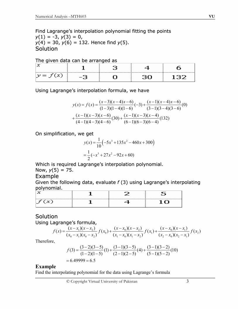
Numerical Analysis –MTH603 VU
© Copyright Virtual University of Pakistan 3
FFiinndd LLaaggrraannggee’’ss iinntteerrppoollaattiioonn ppoollyynnoommiiaall ffiittttiinngg tthhee ppooiinnttss
yy((11)) == --33,, yy((33)) == 00,,
yy((44)) == 3300,, yy((66)) == 113322.. HHeennccee ffiinndd yy((55))..
SSoolluuttiioonn
TThhee ggiivveenn ddaattaa ccaann bbee aarrrraannggeedd aass
UUssiinngg LLaaggrraannggee’’ss iinntteerrppoollaattiioonn ffoorrmmuullaa,, wwee hhaavvee
( 3)( 4) 6) ( 1)( 4) 6)( ) ( ) ( 3) (0)
(1 3)(1 4)(1 6) (3 1)(3 4)(3 6)
( 1)( 3)( 6) ( 1)( 3)( 4)(30) (132)
(4 1)(4 3)(4 6) (6 1)(6 3)(6 4)
x x x x x xy x f x
x x x x x x
! ! "
" "
OOnn ssiimmpplliiffiiccaattiioonn,, wwee ggeett
# $3 2
3 2
1( ) 5 135 460 300
10
1( 27 92 60)
2
y x x x x
x x x
! " "
! " "
WWhhiicchh iiss rreeqquuiirreedd LLaaggrraannggee’’ss iinntteerrppoollaattiioonn ppoollyynnoommiiaall..
NNooww,, yy((55)) == 7755..
EExxaammppllee GGiivveenn tthhee ffoolllloowwiinngg ddaattaa,, eevvaalluuaattee ff ((33)) uussiinngg LLaaggrraannggee’’ss iinntteerrppoollaattiinngg
ppoollyynnoommiiaall..
SSoolluuttiioonn UUssiinngg LLaaggrraannggee’’ss ffoorrmmuullaa,,
0 2 0 11 20 1 2
0 1 0 2 1 0 1 2 2 0 2 1
( )( ) ( )( )( )( )( ) ( ) ( ) ( )
( )( ) ( )( ) ( )( )
x x x x x x x xx x x xf x f x f x f x
x x x x x x x x x x x x
! " "
Therefore,
(3 2)(3 5) (3 1)(3 5) (3 1)(3 2)(3) (1) (4) (10)
(1 2)(1 5) (2 1)(2 5) (5 1)(5 2)
6.49999 6.5
f
! " "
! !
Example Find the interpolating polynomial for the data using Lagrange’s formula

Numerical Analysis –MTH603 VU
© Copyright Virtual University of Pakistan 4
Solution: As Lagrange’s formula for interpolating polynomial is given by,
# $# $# $# $
# $# $# $# $
# $# $# $# $
# $# $# $# $
# $ # $# $# $# $
# $ # $# $# $# $
# $
# $ # $ # $
1 2 0 2 0 1
0 1 2
0 1 0 2 1 0 1 2 2 0 2 1
2 2 2
2 2 2
( ) ( ) ( ) ( ) ( )
2 4 1 4 1 23 5 4
1 2 1 4 2 1 2 4 4 1 4 2
3 5 42 8 3 4 3 2
5 6 30
3 6 24 5 15 20 4 12
5 5 5 6 6 6 30 30
x x x x x x x x x x x xy x f x f x f x f x
x x x x x x x x x x x x
x x x x x x
x x x x x x
x x x x x x
! ! " "
" " ! " "
" "
! " " "
! " " "
2
2
8
30
3 5 4 6 15 12 24 20 8
5 6 30 5 6 30 5 6 30
47 33 118
30 10 15
.
x x
x x
Which is the required polynomial
% & % & % &! " " " " ' ( ' ( ' () * ) * ) *
! "
x 1 2 -4
F(x) 3 -5 -4

Numerical Analysis –MTH603 VU
© Copyright Virtual University of Pakistan 1
DDIIVVIIDDEEDD DDIIFFFFEERREENNCCEESS LLeett uuss aassssuummee tthhaatt tthhee ffuunnccttiioonn yy == ff ((xx)) iiss kknnoowwnn ffoorr sseevveerraall vvaalluueess ooff xx,, ((xx
ii,, yy
ii)),, ffoorr
ii==00,,11,,....nn.. TThhee ddiivviiddeedd ddiiffffeerreenncceess ooff oorrddeerrss 00,, 11,, 22,, ……,, nn aarree nnooww ddeeffiinneedd rreeccuurrssiivveellyy aass::
0 0 0[ ] ( )y x y x y
iiss tthhee zzeerroo--tthh oorrddeerr ddiivviiddeedd ddiiffffeerreennccee
TThhee ffiirrsstt oorrddeerr ddiivviiddeedd ddiiffffeerreennccee iiss ddeeffiinneedd aass
1 00 1
1 0
[ , ]y y
y x xx x
!
!
SSiimmiillaarrllyy,, tthhee hhiigghheerr oorrddeerr ddiivviiddeedd ddiiffffeerreenncceess aarree ddeeffiinneedd iinn tteerrmmss ooff lloowweerr oorrddeerr ddiivviiddeedd
ddiiffffeerreenncceess bbyy tthhee rreellaattiioonnss ooff tthhee ffoorrmm
1 2 0 10 1 2
2 0
[ , ] [ , ][ , , ]
y x x y x xy x x x
x x
!
!
Generally,
" #0
0 1 1 2 0 1 1
1[ , , , ] [ , , , ] [ , , , ]n n n
n
y x x x y x x x y x x xx x
! !!
SSttaannddaarrdd ffoorrmmaatt ooff tthhee DDiivviiddeedd DDiiffffeerreenncceess
WWee ccaann eeaassiillyy vveerriiffyy tthhaatt tthhee ddiivviiddeedd ddiiffffeerreennccee iiss aa ssyymmmmeettrriicc ffuunnccttiioonn ooff iittss aarrgguummeennttss..
TThhaatt iiss,,
0 11 0 0 1
0 1 1 0
[ , ] [ , ]y y
y x x y x xx x x x
$! !
Now
1 2 0 10 1 2
2 0
1 02 1
2 0 2 1 1 0
[ , ] [ , ][ , , ]
1
y x x y x xy x x x
x x
y yy y
x x x x x x
!
!
% &!! !' (
! ! !) *

Numerical Analysis –MTH603 VU
© Copyright Virtual University of Pakistan 2
Therefore
0 1 20 1 2
0 1 0 2 1 0 1 2 2 0 2 1
[ , , ]( )( ) ( )( ) ( )( )
y y yy x x x
x x x x x x x x x x x x $ $
! ! ! ! ! !
TThhiiss iiss ssyymmmmeettrriicc ffoorrmm,, hheennccee ssuuggggeessttss tthhee ggeenneerraall rreessuulltt aass
0 10
0 1 0 1 0 1 0 1
[ , , ]( ) ( ) ( ) ( ) ( ) ( )
kk
k k k k k
y yyy x x
x x x x x x x x x x x x !
$ $ $! ! ! ! ! !
!
! ! !
OORR
0
0
0
[ ,..., ]
( )
ki
k ki
i jii j
yy x x
x x
+
, !
-
EExxaammppllee:: CCoonnssttrruucctt tthhee NNeewwttoonn’’ss ddiivviiddeedd ddiiffffeerreennccee ttaabbllee ffoorr vvaalluueess ooff xx==11,,22,,33,,44,,55,,66
aanndd ff((xx))== --33,,00,,1155,,4488,,110055,,119922..
SSoolluuttiioonn::
NNEEWWTTOONN’’SS DDIIVVIIDDEEDD DDIIFFFFEERREENNCCEE IINNTTEERRPPOOLLAATTIIOONN
FFOORRMMUULLAA LLeett yy == ff ((xx)) bbee aa ffuunnccttiioonn wwhhiicchh ttaakkeess vvaalluueess yy
00,, yy
11,, ……,, yy
nn ccoorrrreessppoonnddiinngg ttoo xx == xx
ii,, ii == 00,,
11,,……,, nn.. WWee cchhoooossee aann iinntteerrppoollaattiinngg ppoollyynnoommiiaall,, iinntteerrppoollaattiinngg aatt xx == xxii,, ii == 00,, 11,, ……,, nn iinn
tthhee ffoolllloowwiinngg ffoorrmm
0 1 0 2 0 1
0 1 1
( ) ( ) ( )( )
( )( ) ( )n n
y f x a a x x a x x x x
a x x x x x x !
$ ! $ ! !
$ $ ! ! !! !
x F(x) 1st
difference
2nd
difference
3rd
difference
1 -3 15-3/3-
1=6
2 0 0-(-3)=3 33-15/4-2
=9
9-6/4-1=1
3 15 15-0=15 57-33/5-3
=12
12-9/5-
2=1
4 48 48-15=33 87-57/6-4
=15
15-12/6-3
=1
5 105 105-48=57
6 192 192-105=87

Numerical Analysis –MTH603 VU
© Copyright Virtual University of Pakistan 3
HHeerree,, tthhee ccooeeffffiicciieennttss aakk aarree ssoo cchhoosseenn aass ttoo ssaattiissffyy aabboovvee eeqquuaattiioonn bbyy tthhee ((nn ++ 11)) ppaaiirrss
((xxii,, yy
ii))..
TThhuuss,, wwee hhaavvee
0 0 0 0
1 1 1 0 1 1 0
2 2 2 0 1 2 0 2 2 0 2 1
0 1 0 2 0 1 0 1
( ) ( )
( ) ( ) ( )
( ) ( ) ( ) ( )( )
( ) ( )( ) ( ) ( )n n n n n n n n
y x f x y a
y x f x y a a x x
y x f x y a a x x a x x x x
y a a x x a x x x x a x x x x
! ! ! "#! ! ! $ ##
! ! ! $ $ %##
! $ $ $ $ #&
TThhee ccooeeffffiicciieennttss aa00,, aa11,, ……,, aa
nn ccaann bbee eeaassiillyy oobbttaaiinneedd ffrroomm tthhee aabboovvee ssyysstteemm ooff
eeqquuaattiioonnss,, aass tthheeyy ffoorrmm aa lloowweerr ttrriiaanngguullaarr mmaattrriixx..
TThhee ffiirrsstt eeqquuaattiioonn ggiivveess
0 0 0( )a y x y! !
TThhee sseeccoonndd eeqquuaattiioonn ggiivveess
1 01 0 1
1 0
[ , ]y y
a y x xx x
! !
TThhiirrdd eeqquuaattiioonn yyiieellddss
2 0 2 0 0 12
2 0 2 1
( ) [ , ]
( )( )
y y x x y x xa
x x x x
!
WWhhiicchh ccaann bbee rreewwrriitttteenn aass
1 02 1 1 0 2 0 0 1
1 0
2
2 0 2 1
( ) ( ) [ , ]
( )( )
y yy y x x x x y x x
x xa
x x x x
' () * $ + ,- .
/ 01 2!
TThhaatt iiss
2 1 0 1 1 2 1 2 0 1
2
2 0 2 1 2 0
[ , ]( ) [ , ] [ , ]
( )( )
y y y x x x x y x x y x xa
x x x x x x
$ ! !
TThhuuss,, iinn tteerrmmss ooff sseeccoonndd oorrddeerr ddiivviiddeedd ddiiffffeerreenncceess,, wwee hhaavvee
2 0 1 2[ , , ]a y x x x!
SSiimmiillaarrllyy,, wwee ccaann sshhooww tthhaatt
NNeewwttoonn’’ss ddiivviiddeedd ddiiffffeerreennccee iinntteerrppoollaattiioonn ffoorrmmuullaa ccaann bbee wwrriitttteenn aass
0 0 0 1 0 1 0 1 2
0 1 1 0 1
( ) ( ) [ , ] ( )( ) [ , , ]
( )( ) ( ) [ , ,..., ]n n
y f x y x x y x x x x x x y x x x
x x x x x x y x x x
! ! $ $
$ $ !
NNeewwttoonn’’ss ddiivviiddeedd ddiiffffeerreenncceess ccaann aallssoo bbee eexxpprreesssseedd iinn tteerrmmss ooff ffoorrwwaarrdd,, bbaacckkwwaarrdd aanndd
cceennttrraall ddiiffffeerreenncceess.. TThheeyy ccaann bbee eeaassiillyy ddeerriivveedd..
AAssssuummiinngg eeqquuii--ssppaacceedd vvaalluueess ooff aabbsscciissssaa,, wwee hhaavvee

Numerical Analysis –MTH603 VU
© Copyright Virtual University of Pakistan 4
1 0 00 1
1 0
[ , ]y y y
y x xx x h
3! !
012
1 2 0 1 00 1 2 2
2 0
[ , ] [ , ][ , , ]
2 2!
yyy x x y x x yh hy x x x
x x h h
33
3! ! !
BByy iinndduuccttiioonn,, wwee ccaann iinn ggeenneerraall aarrrriivvee aatt tthhee rreessuulltt
00 1[ , , , ]
!
n
n n
yy x x x
n h
3!!
SSiimmiillaarrllyy,,
1 0 10 1
1 0
[ , ]y y y
y x xx x h
4! !
2 12
1 2 0 1 20 1 2 2
2 0
[ , ] [ , ][ , , ]
2 2!
y yy x x y x x yh hy x x x
x x h h
4 4
4! ! !
IInn GGeenneerraall,,wwee hhaavvee
0 1[ , ,..., ]!
n
nn n
yy x x x
n h
4!
AAllssoo,, iinn tteerrmmss ooff cceennttrraall ddiiffffeerreenncceess,, wwee hhaavvee
1 0 1/ 20 1
1 0
[ , ]y y y
y x xx x h
5 ! !
3/ 2 1/ 22
1 2 0 1 10 1 2 2
2 0
[ , ] [ , ][ , , ]
2 2!
y yy x x y x x yh hy x x x
x x h h
5 55
! ! !
IInn ggeenneerraall,, wwee hhaavvee tthhee ffoolllloowwiinngg ppaatttteerrnn
2
0 1 2 2
2 1
(1/ 2)
0 1 2 1 2 1
[ , ,..., ](2 )!
[ , ,..., ](2 1)!
m
mm m
m
m
m m
yy x x x
m h
yy x x x
m h
5
5 $$
$ $
"! #
#%#! #$ &

Numerical Analysis –MTH603 VU
© Copyright Virtual University of Pakistan 1
EExxaammppllee
FFiinndd tthhee iinntteerrppoollaattiinngg ppoollyynnoommiiaall bbyy ((ii)) LLaaggrraannggee’’ss ffoorrmmuullaa aanndd
((iiii)) NNeewwttoonn’’ss ddiivviiddeedd ddiiffffeerreennccee ffoorrmmuullaa ffoorr tthhee ffoolllloowwiinngg ddaattaa.. HHeennccee sshhooww tthhaatt tthheeyy
rreepprreesseenntt tthhee ssaammee iinntteerrppoollaattiinngg ppoollyynnoommiiaall..
SSoolluuttiioonn TThhee ddiivviiddeedd ddiiffffeerreennccee ttaabbllee ffoorr tthhee ggiivveenn ddaattaa iiss ccoonnssttrruucctteedd aass ffoolllloowwss::
ii)) LLaaggrraannggee’’ss iinntteerrppoollaattiioonn ffoorrmmuullaa ggiivveess
( 1)( 2)( 4) ( 0)( 2)( 4)
( ) (1) (1)( 1)( 2)( 4) (1 0)(1 2)(1 4)
x x x x x xy f x
! ! "
( 0)( 1)( 4) ( 0)( 1)( 2)
(2) (5)(2)(2 1)(2 4) 4(4 1)(4 2)
x x x x x x " "
3 2 3 2 3 2( 7 14 8) 6 8 5 4
8 3 2
x x x x x x x x x " " "! "
3 25( 3 2 )
24
x x x ""
3 23 2
112 4 3
x xx! " "
((iiii)) NNeewwttoonn’’ss ddiivviiddeedd ddiiffffeerreennccee ffoorrmmuullaa ggiivveess
1 1
( ) 1 ( 0)(0) ( 0)( 1) ( 0)( 1)( 2)2 12
y f x x x x x x x# $ # $! ! " " " % & % &' ( ' (
3 23 2
112 4 3
x xx! " "
WWee oobbsseerrvvee tthhaatt tthhee iinntteerrppoollaattiinngg ppoollyynnoommiiaall bbyy bbootthh LLaaggrraannggee’’ss aanndd NNeewwttoonn’’ss ddiivviiddeedd
ddiiffffeerreennccee ffoorrmmuullaaee iiss oonnee aanndd tthhee ssaammee..
xx 00 11 22 44
yy 11 11 22 55
XX YY 11sstt DD..DD 22
nndd DD..DD 33
rrdd DD..DD
00 11
11 11 00
22 22 11 11//22 --11//22
44 55 33//22 11//66

Numerical Analysis –MTH603 VU
© Copyright Virtual University of Pakistan 2
NNoottee!!
NNeewwttoonn’’ss ffoorrmmuullaa iinnvvoollvveess lleessss nnuummbbeerr ooff aarriitthhmmeettiicc ooppeerraattiioonnss tthhaann tthhaatt ooff LLaaggrraannggee’’ss..
EExxaammppllee UUssiinngg NNeewwttoonn’’ss ddiivviiddeedd ddiiffffeerreennccee ffoorrmmuullaa,, ffiinndd tthhee qquuaaddrraattiicc eeqquuaattiioonn ffoorr tthhee ffoolllloowwiinngg
ddaattaa..
HHeennccee ffiinndd yy ((22))..
SSoolluuttiioonn::
TThhee ddiivviiddeedd ddiiffffeerreennccee ttaabbllee ffoorr tthhee ggiivveenn ddaattaa iiss ccoonnssttrruucctteedd aass::
XX YY 11sstt DD..DD 22
nndd DD..DD
00 22
11 11 --11 11//22
44 44 11
NNooww,, uussiinngg NNeewwttoonn’’ss ddiivviiddeedd ddiiffffeerreennccee ffoorrmmuullaa,, wwee hhaavvee
2
12 ( 0)( 1) ( 0)( 1)
2
1( 3 4)
2
y x x x
x x
# $! " " % &' (
! "
HHeennccee,, yy ((22)) == 11..
EExxaammppllee
Find the equation of a cubic curve which passes through the points (4 , -43) , (7 , 83) , (9 ,
327) and (12 , 1053) using Dividing Difference Formula.
SSoolluuttiioonn The Newton’s divided difference table is given by
X Y 1st divided
difference
2nd
divided
difference
3rd
divided
difference
4 -43
7 83 42
9 327 122 16
12 1053 242 24 1
XX 00 11 44
YY 22 11 44
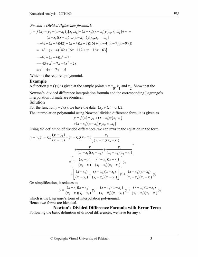
Numerical Analysis –MTH603 VU
© Copyright Virtual University of Pakistan 3
) *
0 0 0 1 0 1 0 1 2
0 1 1 0 1
2
'
( ) ( ) [ , ] ( )( ) [ , , ]
( )( ) ( ) [ , ,..., ]
43 ( 4)(42) ( 4)( 7)(16) ( 4)( 7)( 9)(1)
43 ( 4) 42 16 112 16 63
n n
Newton s Divided Difference formula is
y f x y x x y x x x x x x y x x x
x x x x x x y x x x
x x x x x x
x x x x
! ! " " " "
! " " "
! " " " "
!
!
2
3 2
3 2
43 ( 4)( 7)
43 7 4 28
4 7 15
Which is the required polynomial.
x x
x x x
x x x
"
! " "
!
EExxaammppllee AA ffuunnccttiioonn yy == ff ((xx)) iiss ggiivveenn aatt tthhee ssaammppllee ppooiinnttss xx == xx
00,, xx
11 aanndd xx
22.. SShhooww tthhaatt tthhee
NNeewwttoonn’’ss ddiivviiddeedd ddiiffffeerreennccee iinntteerrppoollaattiioonn ffoorrmmuullaa aanndd tthhee ccoorrrreessppoonnddiinngg LLaaggrraannggee’’ss
iinntteerrppoollaattiioonn ffoorrmmuullaa aarree iiddeennttiiccaall..
SSoolluuttiioonn
FFoorr tthhee ffuunnccttiioonn yy == ff ((xx)),, wwee hhaavvee tthhee ddaattaa ( , ), 0,1, 2.i ix y i !
TThhee iinntteerrppoollaattiioonn ppoollyynnoommiiaall uussiinngg NNeewwttoonn’’ ddiivviiddeedd ddiiffffeerreennccee ffoorrmmuullaa iiss ggiivveenn aass
0 0 0 1
0 1 0 1 2
( ) ( ) [ , ]
( )( ) [ , , ]
y f x y x x y x x
x x x x y x x x
! ! "
"
UUssiinngg tthhee ddeeffiinniittiioonn ooff ddiivviiddeedd ddiiffffeerreenncceess,, wwee ccaann rreewwrriittee tthhee eeqquuaattiioonn iinn tthhee ffoorrmm
1 0 00 0 0 1
1 0 0 1 0 2
( )( ) ( )( )
( ) ( )( )
y y yy y x x x x x x
x x x x x x
+ ! " , -
1 2
1 0 1 2 2 0 2 1( )( ) ( )( )
y y
x x x x x x x x
." " / 0
0 0 10
0 1 0 1 0 2
( ) ( )( )1
( ) ( )( )
x x x x x xy
x x x x x x
+ . ! ", / - 0
0 0 1 0 11 2
1 0 1 0 1 2 2 0 2 1
( ) ( )( ) ( )( )
( ) ( )( ) ( )( )
x x x x x x x x x xy y
x x x x x x x x x x
+ . " " ", / - 0
OOnn ssiimmpplliiffiiccaattiioonn,, iitt rreedduucceess ttoo
0 2 0 11 20 1 2
0 1 0 2 1 0 1 2 2 0 2 1
( )( ) ( )( )( )( )
( )( ) ( )( ) ( )( )
x x x x x x x xx x x xy y y y
x x x x x x x x x x x x
! " "
wwhhiicchh iiss tthhee LLaaggrraannggee’’ss ffoorrmm ooff iinntteerrppoollaattiioonn ppoollyynnoommiiaall..
HHeennccee ttwwoo ffoorrmmss aarree iiddeennttiiccaall..
NNeewwttoonn’’ss DDiivviiddeedd DDiiffffeerreennccee FFoorrmmuullaa wwiitthh EErrrroorr TTeerrmm FFoolllloowwiinngg tthhee bbaassiicc ddeeffiinniittiioonn ooff ddiivviiddeedd ddiiffffeerreenncceess,, wwee hhaavvee ffoorr aannyy xx

Numerical Analysis –MTH603 VU
© Copyright Virtual University of Pakistan 4
0 0 0
0 0 1 1 0 1
0 1 0 1 2 2 0 1 2
0 1 0 1 0
( ) ( ) [ , ]
[ , ] [ , ] ( ) [ , , ]
[ , , ] [ , , ] ( ) [ , , , ]
[ , ,..., ] [ , ,..., ] ( ) [ , ,..., ]n n n n
y x y x x y x x
y x x y x x x x y x x x
y x x x y x x x x x y x x x x
y x x x y x x x x x y x x x
! " 12! " 22
! " 322
! " 24
MMuullttiippllyyiinngg tthhee sseeccoonndd EEqquuaattiioonn bbyy ((xx –– xx00)),, tthhiirrdd bbyy ((xx –– xx
00))((xx –– xx
11)) aanndd ssoo oonn,,
aanndd tthhee llaasstt bbyy
((xx –– xx00))((xx –– xx
11)) …… ((xx –– xx
nn--11)) aanndd aaddddiinngg tthhee rreessuullttiinngg eeqquuaattiioonnss,, wwee oobbttaaiinn
0 0 0 1 0 1 0 1 2( ) ( ) [ , ] ( )( ) [ , , ]y x y x x y x x x x x x y x x x! " " "
0 1 1 0 1( )( ) ( ) [ , ,..., ] ( )n nx x x x x x y x x x x5 " "
Where
0 1 0( ) ( )( ) ( ) [ , ,..., ]n nx x x x x x x y x x x5 !
PPlleeaassee nnoottee tthhaatt ffoorr xx == xx00,, xx
11,, ……,, xx
nn,, tthhee eerrrroorr tteerrmm ( )x5 vvaanniisshheess

Numerical Analysis –MTH603 VU
© Copyright Virtual University of Pakistan 1
EErrrroorr TTeerrmm iinn IInntteerrppoollaattiioonn FFoorrmmuullaaee WWee kknnooww,, iiff yy ((xx)) iiss aapppprrooxxiimmaatteedd bbyy aa ppoollyynnoommiiaall PP
nn ((xx)) ooff ddeeggrreeee nn tthheenn tthhee eerrrroorr iiss
ggiivveenn bbyy
( ) ( ) ( ),nx y x P x ! "
Where
0 1 0( ) ( )( ) ( ) [ , ,..., ]n nx x x x x x x y x x x ! " " "
AAlltteerrnnaattiivveellyy iitt iiss aallssoo eexxpprreesssseedd aass
0( ) ( ) [ , ,..., ] ( )nx x y x x x K x ! # ! #
NNooww,, ccoonnssiiddeerr aa ffuunnccttiioonn FF ((xx)),, ssuucchh tthhaatt
( ) ( ) ( ) ( )nF x y x P x K x! " " #
DDeetteerrmmiinnee tthhee ccoonnssttaanntt KK iinn ssuucchh aa wwaayy tthhaatt FF((xx)) vvaanniisshheess ffoorr xx == xx00,, xx
11,, ……,, xx
nn aanndd aallssoo
ffoorr aann aarrbbiittrraarriillyy cchhoosseenn ppooiinntt x ,, wwhhiicchh iiss ddiiffffeerreenntt ffrroomm tthhee ggiivveenn ((nn ++ 11)) ppooiinnttss..
LLeett II ddeennootteess tthhee cclloosseedd iinntteerrvvaall ssppaannnneedd bbyy tthhee vvaalluueess 0 ,..., , .nx x x TThheenn FF ((xx)) vvaanniisshheess
((nn ++ 22)) ttiimmeess iinn tthhee iinntteerrvvaall II..
BByy RRoollllee’’ss tthheeoorreemm ( )F x$ vvaanniisshheess aatt lleeaasstt ((nn ++ 11)) ttiimmeess iinn tthhee iinntteerrvvaall II,, ( )F x$$ aatt
lleeaasstt nn ttiimmeess,, aanndd ssoo oonn..
EEvveennttuuaallllyy,, wwee ccaann sshhooww tthhaatt ( 1) ( )nF x%
vvaanniisshheess aatt lleeaasstt oonnccee iinn tthhee iinntteerrvvaall II,, ssaayy aatt
x &! TThhuuss,, wwee oobbttaaiinn
( 1) ( 1) ( 1)0 ( ) ( ) ( )n n n
ny P K& & &% % %! " " #
SSiinnccee PPnn((xx)) iiss aa ppoollyynnoommiiaall ooff ddeeggrreeee nn,, iittss ((nn ++ 11))tthh ddeerriivvaattiivvee iiss zzeerroo.. AAllssoo,, ffrroomm tthhee
ddeeffiinniittiioonn ooff ( )x'
( 1) ( ) ( 1)!.n x n%# ! %
TThheerreeffoorree wwee ggeett
( 1) ( )
( 1)!
nyK
n
&%
!%
HHeennccee
( 1) ( )
( ) ( ) ( ) ( )( 1)!
n
n
yx y x P x x
n
&
%
! " ! #%
ffoorr ssoommee iinn tthhee iinntteerrvvaall II..
TThhuuss tthhee eerrrroorr ccoommmmiitttteedd iinn rreeppllaacciinngg yy ((xx)) bbyy eeiitthheerr NNeewwttoonn’’ss ddiivviiddeedd ddiiffffeerreennccee
ffoorrmmuullaa oorr bbyy aann iiddeennttiiccaall LLaaggrraannggee’’ss ffoorrmmuullaa iiss
( 1)
0
( )( ) ( ) [ , ,..., ] ( )
( 1)!
n
n
yx x y x x x x
n
&
%
! # ! #%

Numerical Analysis –MTH603 VU
© Copyright Virtual University of Pakistan 2
IINNTTEERRPPOOLLAATTIIOONN IINN TTWWOO DDIIMMEENNSSIIOONNSS
LLeett uu bbee aa ppoollyynnoommiiaall ffuunnccttiioonn iinn ttwwoo vvaarriiaabblleess,, ssaayy xx aanndd yy,, iinn ppaarrttiiccuullaarr qquuaaddrraattiicc iinn xx
aanndd ccuubbiicc iinn yy,, wwhhiicchh iinn ggeenneerraall ccaann bbee wwrriitttteenn aass
2
0 1 2 3
2 3 2 2
4 5 6 7 8
3 2 2 3 2
9 10 11
( , )u f x y a a x a y a x
a xy a y a y a y x a yx
a y x a y x a y x
! ! % % %
% % % % %
% % %
TThhiiss rreellaattiioonn iinnvvoollvveess mmaannyy tteerrmmss.. IIff wwee hhaavvee ttoo wwrriittee aa rreellaattiioonn iinnvvoollvviinngg tthhrreeee oorr mmoorree
vvaarriiaabblleess,, eevveenn llooww ddeeggrreeee ppoollyynnoommiiaallss ggiivvee rriissee ttoo lloonngg eexxpprreessssiioonnss.. IIff nneecceessssaarryy,, wwee
ccaann cceerrttaaiinnllyy wwrriittee,, bbuutt ssuucchh ccoommpplliiccaattiioonnss ccaann bbee aavvooiiddeedd bbyy hhaannddlliinngg eeaacchh vvaarriiaabbllee
sseeppaarraatteellyy..
IIff wwee lleett xx,, aa ccoonnssttaanntt,, ssaayy xx == cc,, tthhee eeqquuaattiioonn ssiimmpplliiffiieess ttoo tthhee ffoorrmm
2 3
0 1 2 3x cu b b y b y b y!! ! % % %
NNooww wwee aaddoopptt tthhee ffoolllloowwiinngg pprroocceedduurree ttoo iinntteerrppoollaattee aatt aa ppooiinntt ((11,, mm)) iinn aa ttaabbllee ooff ttwwoo
vvaarriiaabblleess,, bbyy ttrreeaattiinngg oonnee vvaarriiaabbllee aa ccoonnssttaanntt ssaayy xx == xx11.. TThhee pprroobblleemm rreedduucceess ttoo tthhaatt ooff aa
ssiinnggllee vvaarriiaabbllee iinntteerrppoollaattiioonn..
AAnnyy oonnee ooff tthhee mmeetthhooddss ddiissccuusssseedd iinn pprreecceeddiinngg sseeccttiioonnss ccaann tthheenn bbee aapppplliieedd ttoo ggeett
ff ((xx11,, mm)).. TThheenn wwee rreeppeeaatt tthhiiss pprroocceedduurree ffoorr vvaarriioouuss vvaalluueess ooff xx ssaayy xx == xx
22,, xx
33,, ……,, xx
nn
kkeeeeppiinngg yy ccoonnssttaanntt.. TThhuuss,, wwee ggeett aa nneeww ttaabbllee wwiitthh yy ccoonnssttaanntt aatt tthhee vvaalluuee yy == mm aanndd wwiitthh
xx vvaarryyiinngg.. WWee ccaann tthheenn iinntteerrppoollaattee aatt xx == 11..
EExxaammppllee
TTaabbuullaattee tthhee vvaalluueess ooff tthhee ffuunnccttiioonn ff ((xx)) == xx22++yy
22--yy
ffoorr xx == 00,,11,,22,,33,,44 aanndd yy == 00,,11,,22,,33,,44..
UUssiinngg tthhee ttaabbllee ooff tthhee vvaalluueess,, ccoommppuuttee ff((22..55,, 33..55)) bbyy nnuummeerriiccaall ddoouubbllee iinntteerrppoollaattiioonn
SSoolluuttiioonn TThhee vvaalluueess ooff tthhee ffuunnccttiioonn ffoorr tthhee ggiivveenn vvaalluueess ooff tthhee ggiivveenn vvaalluueess ooff xx aanndd yy aarree ggiivveenn iinn
tthhee ffoolllloowwiinngg ttaabbllee
XX ………….... YY …………....
00 11 22 33 44
00 00 00 22 66 1122

Numerical Analysis –MTH603 VU
© Copyright Virtual University of Pakistan 3
CCoonntt!! UUssiinngg qquuaaddrraattiicc iinntteerrppoollaattiioonn iinn bbootthh xx aanndd yy ddiirreeccttiioonnss wwee nneeeedd ttoo ccoonnssiiddeerr tthhrreeee
ppooiinnttss iinn xx aanndd yy ddiirreeccttiioonnss.. TToo ssttaarrtt wwiitthh wwee hhaavvee ttoo ttrreeaatt oonnee vvaarriiaabbllee aass ccoonnssttaanntt,, ssaayy xx..
KKeeeeppiinngg xx == 22..55,, yy == 33..55 aass nneeaarr tthhee cceenntteerr ooff tthhee sseett,, wwee cchhoooossee tthhee ttaabbllee ooff vvaalluueess
ccoorrrreessppoonnddiinngg ttoo xx == 11,,22,, 33 aanndd yy == 22,, 33,, 44..
CCoonntt!! TThhee rreeggiioonn ooff ffiitt ffoorr tthhee ccoonnssttrruuccttiioonn ooff oouurr iinntteerrppoollaattiioonn ppoollyynnoommiiaall iiss sshhoowwnn iinn
ddiiffffeerreenntt ccoolloorr iinn tthhee ttaabbllee
CCoonntt !! TThhuuss uussiinngg NNeewwttoonn’’ss ffoorrwwaarrdd ddiiffffeerreennccee ffoorrmmuullaa,, wwee hhaavvee
AAtt xx==11
YY ff f( 2 f(
22 33
33 77 44 22
44 1133 66
CCoonntt !!
SSiimmiillaarrllyy
AAtt xx==22
YY ff f( 2 f(
11 11 11 33 77 1133
22 44 44 66 1100 1166
33 99 99 1111 1155 2211
44 1166 1166 1188 2222 2288
XX ……………….. YY ……………………
00 11 22 33 44
00 00 00 22 66 1122
11 11 11 33 77 1133
22 44 44 66 1100 1166
33 99 99 1111 1155 2211
44 1166 1166 1188 2222 2288
Y f

Numerical Analysis –MTH603 VU
© Copyright Virtual University of Pakistan 4
22 66
33 1100 44 22
44 1166 66
CCoonntt !! SSiimmiillaarrllyy
AAtt xx==33
YY ff f( 2 f(
22 1111
33 1155 44 22
44 2211 66
0 3.5 21.5
1
y ywith p
h
" "! ! !
CCoonntt !!
0 3.5 21.5
1
y ywith p
h
" "! ! !
2
0 0 0
( 1)(1,3.5)
2!
(1.5)(0.5)3 (1.5)(4) (2) 9.75
2
p pf f p f f
"! % ( % (
! % % !
CCoonntt !!
(1.5)(0.5)(2,3.5) 6 (1.5)(4) (2) 12.75
2
(1.5)(0.5)(3,3.5) 11 (1.5)(4) (2) 17.75
2
f
f
! % % !
! % % !
CCoonntt !! TThheerreeffoorree wwee aarrrriivvee aatt tthhee ffoolllloowwiinngg rreessuulltt
AAtt xx==33..55
YY ff f( 2 f(
11 99..7755
22 1122..7755 33 22
33 1177..7755 55

Numerical Analysis –MTH603 VU
© Copyright Virtual University of Pakistan 5
CCoonntt !!
2.5 1
1.51
Now defining p"
! !
(1.5)(0.5)
(2.5,3.5) 9.75 (1.5)(3) (2) 152
f ! % % !
CCoonntt !!
FFrroomm tthhee ffuunnccttiioonnaall rreellaattiioonn,, wwee aallssoo ffiinndd tthhaatt
2 2(2.5,3.5) (2.5) (3.5) 3.5 15f ! % " !
And hence no error in interpolation!!!

Numerical Analysis –MTH603 VU
© Copyright Virtual University of Pakistan 1
DDIIFFFFEERREENNTTIIAATTIIOONN UUSSIINNGG DDIIFFFFEERREENNCCEE OOPPEERRAATTOORRSS
IInnttrroodduuccttiioonn CCoonnssiiddeerr aa ffuunnccttiioonn ooff ssiinnggllee vvaarriiaabbllee yy == ff ((xx)).. IIff tthhee ffuunnccttiioonn iiss kknnoowwnn aanndd ssiimmppllee,,
wwee ccaann eeaassiillyy oobbttaaiinn iittss ddeerriivvaattiivvee ((ss)) oorr ccaann eevvaalluuaattee iittss ddeeffiinniittee iinntteeggrraall
HHoowweevveerr,, iiff wwee ddoo nnoott kknnooww tthhee ffuunnccttiioonn aass ssuucchh oorr tthhee ffuunnccttiioonn iiss ccoommpplliiccaatteedd aanndd iiss
ggiivveenn iinn aa ttaabbuullaarr ffoorrmm aatt aa sseett ooff ppooiinnttss xx00,,xx11,,……,,xx
nn,, wwee uussee oonnllyy nnuummeerriiccaall mmeetthhooddss ffoorr
ddiiffffeerreennttiiaattiioonn oorr iinntteeggrraattiioonn ooff tthhee ggiivveenn ffuunnccttiioonn..
WWee sshhaallll ddiissccuussss nnuummeerriiccaall aapppprrooxxiimmaattiioonn ttoo ddeerriivvaattiivveess ooff ffuunnccttiioonnss ooff ttwwoo oorr mmoorree
vvaarriiaabblleess iinn tthhee lleeccttuurreess ttoo ffoollllooww wwhheenn wwee sshhaallll ttaallkk aabboouutt ppaarrttiiaall ddiiffffeerreennttiiaall eeqquuaattiioonnss..
IInn wwhhaatt ffoolllloowwss,, wwee sshhaallll ddeerriivvee aanndd iilllluussttrraattee vvaarriioouuss ffoorrmmuullaaee ffoorr nnuummeerriiccaall
ddiiffffeerreennttiiaattiioonn ooff aa ffuunnccttiioonn ooff aa ssiinnggllee vvaarriiaabbllee bbaasseedd oonn ffiinniittee ddiiffffeerreennccee ooppeerraattoorrss aanndd
iinntteerrppoollaattiioonn..
SSuubbsseeqquueennttllyy,, wwee sshhaallll ddeevveelloopp NNeewwttoonn--CCootteess ffoorrmmuullaaee aanndd rreellaatteedd ttrraappeezzooiiddaall rruullee aanndd
SSiimmppssoonn’’ss rruullee ffoorr nnuummeerriiccaall iinntteeggrraattiioonn ooff aa ffuunnccttiioonn..
WWee aassssuummee tthhaatt tthhee ffuunnccttiioonn yy == ff ((xx)) iiss ggiivveenn ffoorr tthhee vvaalluueess ooff tthhee iinnddeeppeennddeenntt vvaarriiaabbllee
xx == xx00 ++ pphh,, ffoorr pp == 00,, 11,, 22,, …… aanndd ssoo oonn.. TToo ffiinndd tthhee ddeerriivvaattiivveess ooff ssuucchh aa ttaabbuullaarr
ffuunnccttiioonn,, wwee pprroocceeeedd aass ffoolllloowwss
CCaassee II::
UUssiinngg ffoorrwwaarrdd ddiiffffeerreennccee ooppeerraattoorr aanndd ccoommbbiinniinngg eeqquuaattiioonnss
( ) ( )E f x f x h !
aanndd
1E" #
log log(1 )hD E ! "
Remember the Differential operator, D is known to represents the property
2
2 "
2
( ) ( ) ( )
( ) ( ) ( )
dDf x f x f x
dx
dD f x f x f x
dx
$% &&'& &(
TThhiiss wwoouulldd mmeeaann tthhaatt iinn tteerrmmss ooff ::
2 3 4 51
2 3 4 5D
h
) *" " " " " # ! # ! #+ ,
- .
Therefore
2 3
0 00 0 0
4 5
0 00
( ) ( )1( ) ( ) ( )
2 3
( ) ( ) ( )
4 5
f x f xDf x f x f x
h
f x f x df x
dx
/ " "% " # !0
1
2" "# ! # 3
4

Numerical Analysis –MTH603 VU
© Copyright Virtual University of Pakistan 2
in other words
2 3 4
0 0 00 0 0
1
2 3 4
y y yDy y y
h
) *" " "% " # ! # !+ ,
- .
AAllssoo,, wwee ccaann eeaassiillyy vveerriiffyy
22 3 4
2
2
1
2 3 4D
h
) *" " " " # ! # !+ ,
- .
2 3 4 5
2
1 11 5
12 6h
) * " #" ! " # " !+ ,- .
2 32 0 0
2 00 02 2 4 5
0 0
111 5
12 6
y yd y
D y ydx h y y
) *" # "+ ,%% + ,! " # " !+ ,- .
CCaassee IIII::
UUssiinngg bbaacckkwwaarrdd ddiiffffeerreennccee ooppeerraattoorr ,, wwee hhaavvee 5
log(1 )hD # #5
OOnn eexxppaannssiioonn,, wwee hhaavvee
2 3 41
2 3 4D
h
) *5 5 5 5# ! ! !+ ,
- .
wwee ccaann aallssoo vveerriiffyy tthhaatt
22 3 4
2
2
1
2 3 4D
h
) *5 5 5 5# ! ! !+ ,
- .
2 3 4 5
2
1 11 5
12 6h
) * 5 !5 ! 5 ! 5 !+ ,- .
Hence
2 3 41
2 3 4
n n n
n n nn
dy Dy y
dx
y y yy
h
%
) *5 5 5 5 # ! ! !+ ,
- .
and 6
2
2 3 4 5
2
1 11 5
12 6
n n
n n n n
y D y
y y y yh
%%
* 5 !5 ! 5 ! 5 ! ,.
TThhee ffoorrmmuullaaee ffoorr DDyy00aanndd DD
22yy00 aarree uusseeffuull ttoo ccaallccuullaattee tthhee ffiirrsstt aanndd sseeccoonndd ddeerriivvaattiivveess aatt
tthhee bbeeggiinnnniinngg ooff tthhee ttaabbllee ooff vvaalluueess iinn tteerrmmss ooff ffoorrwwaarrdd ddiiffffeerreenncceess;; wwhhiillee ffoorrmmuullaaee ffoorr
yy’’nn aanndd yy’’’’
nn

Numerical Analysis –MTH603 VU
© Copyright Virtual University of Pakistan 3
TThhee ffoorrmmuullaaee ffoorr DDyy00aanndd DD
22yy00 aarree uusseeffuull ttoo ccaallccuullaattee tthhee ffiirrsstt aanndd sseeccoonndd ddeerriivvaattiivveess aatt
tthhee bbeeggiinnnniinngg ooff tthhee ttaabbllee ooff vvaalluueess iinn tteerrmmss ooff ffoorrwwaarrdd ddiiffffeerreenncceess;; wwhhiillee ffoorrmmuullaaee ffoorr
yy’’nn aanndd yy’’’’
nn
CCaassee IIIIII:: UUssiinngg cceennttrraall ddiiffffeerreennccee ooppeerraattoorr aanndd ffoolllloowwiinngg tthhee ddeeffiinniittiioonnss ooff
ddiiffffeerreennttiiaall ooppeerraattoorr DD,, cceennttrraall ddiiffffeerreennccee ooppeerraattoorr aanndd tthhee sshhiifftt ooppeerraattoorr EE,, wwee hhaavvee
1/ 2 1/ 2 / 2 / 2
2sinh2
hD hDE E e e
hD
7 # # # #
Therefore, we have
1sinh2 2
hD 7#
But,
3 51
7
1 1 3sinh
2 3 2 4 5
1 3 5
2 4 6 7
x xx x
x
# 8 # !
88 8
# !8 8
UUssiinngg tthhee llaasstt ttwwoo eeqquuaattiioonnss wwee ggeett
353
2 2 6 8 40 32
hD 7 77
) * # ! #+ ,8 8- .
TThhaatt iiss,,
3 51 1 3
24 640D
h7 7 7) * # ! #+ ,- .
Therefore
3 51 1 3
24 640
dy y Dy
dx
y y yh
7 7 7
%
) * # ! #+ ,- .
Also
2 2 4 6
2
1 1 3
12 90D
h7 7 7) * # ! #+ ,- .
Hence
2 2 4 6
2
1 1 1
12 90y D y y y y
h7 7 7) *%% # ! #+ ,- .
FFoorr ccaallccuullaattiinngg tthhee sseeccoonndd
ddeerriivvaattiivvee aatt aann iinntteerriioorr ttaabbuullaarr
ppooiinntt,, wwee uussee tthhee eeqquuaattiioonn

Numerical Analysis –MTH603 VU
© Copyright Virtual University of Pakistan 4
2 2 4 6
2
1 1 3
12 90D
h7 7 7) * # ! #+ ,- .
wwhhiillee ffoorr ccoommppuuttiinngg tthhee ffiirrssttddeerriivvaattiivvee aatt aann iinntteerriioorr ttaabbuullaarr ppooiinntt,, wwee iinn ggeenneerraall uussee
aannootthheerr ccoonnvveenniieenntt ffoorrmm ffoorr DD,, wwhhiicchh iiss ddeerriivveedd aass ffoolllloowwss.. MMuullttiippllyy tthhee rriigghhtt hhaanndd
ssiiddee ooff
3 51 1 3
24 640
dy y Dy y y y
dx h7 7 7) *% # ! #+ ,- .
by
21 ( 4)
9
7!
wwhhiicchh iiss uunniittyy aanndd nnoottiinngg tthhee BBiinnoommiiaall eexxppaannssiioonn
1 2
2 2
4 6
1 11 1
4 8
3 15
128 48 64
7 7
7 7
#) *! # !+ ,- .
# !8
we get
2 4
3 5
1 31
8 128
1 3
24 640
Dh
97 7
7 7 7
) * # ! #+ ,- .
) *# ! #+ ,- .
OOnn ssiimmpplliiffiiccaattiioonn,, wwee oobbttaaiinn
3 51 4
6 120D
h
97 7 7) * # ! #+ ,- .
TThheerreeffoorree tthhee eeqquuaattiioonn ccaann aallssoo bbee wwrriitttteenn iinn aannootthheerr uusseeffuull ffoorrmm aass
3 51 1
6 30y D y y y
h
97 7 7) *% # ! #+ ,- .
TThhee llaasstt ttwwoo eeqquuaattiioonnss ffoorr yy”” aanndd yy’’ rreessppeeccttiivveellyy aarree kknnoowwnn aass SSttiirrlliinngg’’ss ffoorrmmuullaaee ffoorr
ccoommppuuttiinngg tthhee ddeerriivvaattiivveess ooff aa ttaabbuullaarr ffuunnccttiioonn.. SSiimmiillaarr ffoorrmmuullaaee ccaann bbee ddeerriivveedd ffoorr
ccoommppuuttiinngg hhiigghheerr oorrddeerr ddeerriivvaattiivveess ooff aa ttaabbuullaarr ffuunnccttiioonn..
TThhee eeqquuaattiioonn ffoorr yy’’ ccaann aallssoo bbee
wwrriitttteenn aass
2 2 2 2 2 2
3 5 71 (1) (2) (1) (2) (3)
3! 5! 7!y y y y y
h
97 7 7 7/ 2
% # ! # !0 31 4
IInn oorrddeerr ttoo iilllluussttrraattee tthhee uussee ooff ffoorrmmuullaaee ddeerriivveedd ssoo ffaarr,, ffoorr ccoommppuuttiinngg tthhee ddeerriivvaattiivveess ooff aa
ttaabbuullaatteedd ffuunnccttiioonn,, wwee sshhaallll ccoonnssiiddeerr ssoommee eexxaammpplleess iinn tthhee nneexxtt lleeccttuurree..

Numerical Analysis –MTH603 VU
© Copyright Virtual University of Pakistan 5
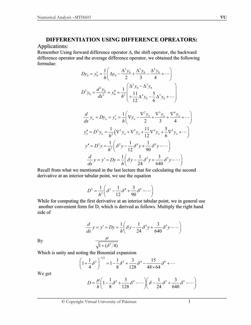
Numerical Analysis –MTH603 VU
© Copyright Virtual University of Pakistan 1
DDIIFFFFEERREENNTTIIAATTIIOONN UUSSIINNGG DDIIFFFFEERREENNCCEE OOPPRREEAATTOORRSS::
AApppplliiccaattiioonnss:: RReemmeemmbbeerr UUssiinngg ffoorrwwaarrdd ddiiffffeerreennccee ooppeerraattoorr ,, tthhee sshhiifftt ooppeerraattoorr,, tthhee bbaacckkwwaarrdd
ddiiffffeerreennccee ooppeerraattoorr aanndd tthhee aavveerraaggee ddiiffffeerreennccee ooppeerraattoorr, wwee oobbttaaiinneedd tthhee ffoolllloowwiinngg
ffoorrmmuullaaee::
2 3 4
0 0 00 0 0
1
2 3 4
y y yDy y y
h
!" " "#$ $ " % & % &' (
) *
2 32 0 0
2 00 02 2 4 5
0 0
111 5
12 6
y yd y
D y ydx h y y
!" % "' (##$ $ $ ' (& " % " &' () *
2 3 4
1
2 3 4
n n nn n n n
y y ydy Dy y y
dx h
!+ + +#$ $ $ + % & & &' (
) *
,2 2 3 4 5
2
1 11 5
12 6n n n n n ny D y y y y y
h
!## $ $ + &+ & + & + & (*
2 2 4 6
2
1 1 1
12 90y D y y y y
h- - - !## $ $ % & %' (
) *
3 51 1 3
24 640
dy y Dy y y y
dx h- - - !#$ $ $ % & %' (
) *
RReeccaallll ffrroomm wwhhaatt wwee mmeennttiioonneedd iinn tthhee llaasstt lleeccttuurree tthhaatt ffoorr ccaallccuullaattiinngg tthhee sseeccoonndd
ddeerriivvaattiivvee aatt aann iinntteerriioorr ttaabbuullaarr ppooiinntt,, wwee uussee tthhee eeqquuaattiioonn
2 2 4 6
2
1 1 3
12 90D
h- - - !$ % & %' (
) *
WWhhiillee ffoorr ccoommppuuttiinngg tthhee ffiirrsstt ddeerriivvaattiivvee aatt aann iinntteerriioorr ttaabbuullaarr ppooiinntt,, wwee iinn ggeenneerraall uussee
aannootthheerr ccoonnvveenniieenntt ffoorrmm ffoorr DD,, wwhhiicchh iiss ddeerriivveedd aass ffoolllloowwss.. MMuullttiippllyy tthhee rriigghhtt hhaanndd
ssiiddee ooff
3 51 1 3
24 640
dy y Dy y y y
dx h- - - !#$ $ $ % & %' (
) *
By 21 ( 4)
.
-&
WWhhiicchh iiss uunniittyy aanndd nnoottiinngg tthhee BBiinnoommiiaall eexxppaannssiioonn
1 2
2 2 4 61 1 3 151 1
4 8 128 48 64- - - -
% !& $ % & % &' ( /) *
We get
2 4 3 51 3 1 31
8 128 24 640D
h
.- - - - - ! !$ % & % % & %' (' (
) *) *

Numerical Analysis –MTH603 VU
© Copyright Virtual University of Pakistan 2
SSiimmpplliiffiiccaattiioonn wwee ggeett
3 51 4
6 120D
h
.- - - !$ % & %' (
) *
TThheerreeffoorree tthhee eeqquuaattiioonn ccaann aallssoo bbee wwrriitttteenn iinn aannootthheerr uusseeffuull ffoorrmm aass
3 51 1
6 30y D y y y
h
.- - - !# $ $ % & %' (
) *
TThhee llaasstt ttwwoo eeqquuaattiioonnss yy”” aannddyy’’ rreessppeeccttiivveellyy aarree kknnoowwnn aass SSttiirrlliinngg’’ss ffoorrmmuullaaee ffoorr
ccoommppuuttiinngg tthhee ddeerriivvaattiivveess ooff aa ttaabbuullaarr ffuunnccttiioonn.. SSiimmiillaarr ffoorrmmuullaaee ccaann bbee ddeerriivveedd ffoorr
ccoommppuuttiinngg hhiigghheerr oorrddeerr ddeerriivvaattiivveess ooff aa ttaabbuullaarr ffuunnccttiioonn..
TThhee eeqquuaattiioonn ffoorr yy’’ ccaann aallssoo bbee wwrriitttteenn aass
2 2 2 2 2 2
3 5 71 (1) (2) (1) (2) (3)
3! 5! 7!y y y y y
h
.- - - -0 1
# $ % & % &2 34 5
IInn oorrddeerr ttoo iilllluussttrraattee tthhee uussee ooff ffoorrmmuullaaee ddeerriivveedd ssoo ffaarr,, ffoorr ccoommppuuttiinngg tthhee
ddeerriivvaattiivveess ooff aa ttaabbuullaatteedd ffuunnccttiioonn,, wwee ccoonnssiiddeerr tthhee ffoolllloowwiinngg eexxaammppllee ::
EExxaammppllee:: CCoommppuuttee (0)f ## aanndd (0.2)f # ffrroomm tthhee ffoolllloowwiinngg ttaabbuullaarr ddaattaa..
SSoolluuttiioonn
SSiinnccee xx == 00 aanndd 00..22 aappppeeaarr aatt aanndd nneeaarr bbeeggiinnnniinngg ooff tthhee ttaabbllee,, iitt iiss aapppprroopprriiaattee ttoo uussee
ffoorrmmuullaaee bbaasseedd oonn ffoorrwwaarrdd ddiiffffeerreenncceess ttoo ffiinndd tthhee ddeerriivvaattiivveess.. TThhee ddiiffffeerreennccee ttaabbllee ffoorr tthhee
ggiivveenn ddaattaa iiss ddeeppiicctteedd bbeellooww::
xx ff((xx)) ( )f x" 2 ( )f x" 3 ( )f x"
4 ( )f x" 5 ( )f x"
00..00 11..0000
00..22 11..1166 00..1166
00..44 33..5566 22..4400 22..2244 55..7766
00..66 1133..9966 1100..4400 88..0000 99..6600 33..8844 00..00
00..88 4411..9966 2288..0000 1177..6600 1133..4444 33..8844
11..00 110011..0000 5599..0044 3311..0044
UUssiinngg ffoorrwwaarrdd ddiiffffeerreennccee ffoorrmmuullaa ffoorr 2 ( ),D f x
ii..ee
xx 00..00 00..22 00..44 00..66 00..88 11..00
FF((xx)) 11..0000 11..1166 33..5566 1133..9966 4411..9966 110011..0000
( )f x" 2 ( )f x"

Numerical Analysis –MTH603 VU
© Copyright Virtual University of Pakistan 3
2 3
2 4 5
2
( ) ( )1 11 5( ) ( ) ( )
12 6
f x f xD f x f x f x
h
0" %" 1$ & " % "2 354
we obtained
2
1 11 5(0) 2.24 5.76 (3.84) (0) 0.0
(02) 12 6f
0 1## $ % & % $2 34 5
AAllssoo,, uussiinngg tthhee ffoorrmmuullaa ffoorr ( )Df x ,, wwee hhaavvee
2 3 41 ( ) ( ) ( )( ) ( )
2 3 4
f x f x f xDf x f x
h
0 1" " "$ " % & %2 3
4 5
HHeennccee,,
1 8.00 9.60 3.84
(0.2) 2.40 3.20.2 2 3 4
f !# $ % & % $' () *
EExxaammppllee FFiinndd (2.2)y# aanndd (2.2)y## ffrroomm tthhee ttaabbllee..
xx 11..44 11..66 11..88 22..00 22..22
YY((xx)) 44..00555522 44..99553300 66..00449966 77..33889911 99..00225500
SSoolluuttiioonn:: SSiinnccee xx==22..22 ooccccuurrss aatt tthhee eenndd ooff tthhee ttaabbllee,, iitt iiss aapppprroopprriiaattee ttoo uussee bbaacckkwwaarrdd ddiiffffeerreennccee
ffoorrmmuullaaee ffoorr ddeerriivvaattiivveess.. TThhee bbaacckkwwaarrdd ddiiffffeerreennccee ttaabbllee ffoorr tthhee ggiivveenn ddaattaa iiss sshhoowwnn
bbeellooww::
xx ff((xx)) y+ 2 y+ 3y+
4 y+
11..44 44..00555522
11..66 44..99553300 00..88997788
11..88 66..00449966 11..00996666 00..11998888 00..00444411
22..00 77..33889911 11..33339955 00..22442299 00..00553355 00..00009944
22..22 99..00225500 11..66335599 00..22996644
UUssiinngg bbaacckkwwaarrdd ddiiffffeerreennccee ffoorrmmuullaaee ffoorr ( )y x# aanndd ( ),y x## wwee hhaavvee
2 3 4
1
2 3 4
n n nn n
y y yy y
h
!+ + +# $ + & & &' (
) *
TThheerreeffoorree,,

Numerical Analysis –MTH603 VU
© Copyright Virtual University of Pakistan 4
1 0.2964 0.0535 0.0094(2.2) 1.6359 5(1.8043) 9.02
0.2 2 3 4y
!# $ & & & $ $' () *
AAllssoo
2 3 4
2
1 11
12n n n ny y y yh
!## $ + &+ & +' () *
TThheerreeffoorree
,2
1 11(2.2) 0.2964 0.0535 (0.0094)
(0.2) 12
25(0.3585) 8.9629
y!## $ & & (*
$ $
EExxaammppllee
Given the table of values, estimate, // (1.3)y
Solution Since x = 1.3 appear at beginning of the table, it is appropriate to use formulae
based on forward differences to find the derivatives. The difference table for the given
data is depicted below:
H=0.2
Using forward difference formula for 2 ( ),D f x
2 2 3 4 5
2
1 11 5( ) ( ) ( ) ( ) ( )
12 6D f x f x f x f x f x
h
10$ " % " & " % "4 35
We obtain
x 1.3 1.5 1.7 1.9 2.1 2.3
y 2.9648 2.6599 2.3333 1.9922 1.6442 1.2969
x y ( )f x" 2 ( )f x" 3 ( )f x" 4 ( )f x" 5 ( )f x"
1.3 2.9648
1.5 2.6599
-0.3049
1.7 2.3333
-0.3266 -0.0217
1.9 1.9922
-0.3411 -0.0145 0.0072
2.1 1.6442
-0.348 -0.0069 0.0076 0.0004
2.3 1.2969 -0.3473 0.0007 0.0076 0 -0.0004

Numerical Analysis –MTH603 VU
© Copyright Virtual University of Pakistan 5
6 7
6 7
2
2
2
2
1 11 5(1.3) -0.0217 0.0072 (0.0004) (-0.0004)
(0.2) 12 6
1(1.3) -0.0217 0.0072 (0.9167)(0.0004) (0.8334)(-0.0004)
(0.2)
1(1.3) -0.0217 0.0072 (0.0003667) (0.0003334)
(0.2)
1(1.3) -0.0
(0.2)
f
f
f
f
0 1## $ % & %2 34 5
## $ % & %
## $ % & &
## $ 6 282] 0.7050$ %
CCaassee IIVV:: DDeerriivvaattiioonn ooff TTwwoo aanndd tthhrreeee ppooiinntt ffoorrmmuullaaee::
RReettaaiinniinngg oonnllyy tthhee ffiirrsstt tteerrmm iinn eeqquuaattiioonn::
2 3 4
0 0 00 0 0
1
2 3 4
y y yDy y y
h
!" " "#$ $ " % & % &' (
) *
wwee ccaann ggeett aannootthheerr uusseeffuull ffoorrmm ffoorr tthhee ffiirrsstt ddeerriivvaattiivvee aass
1 ( ) ( )i i i i ii
y y y y x h y x
h h h
&" % & %$ $ $
SSiimmiillaarrllyy,, bbyy rreettaaiinniinngg oonnllyy tthhee ffiirrsstt tteerrmm iinn EEqqnn..
2 3 4
1
2 3 4
n n nn n n n
y y ydy Dy y y
dx h
!+ + +#$ $ $ + % & & &' (
) *
1 ( ) ( )i i i i ii
y y y y x y x hy
h h h
%+ % % %# $ $ $
AAddddiinngg tthhee llaasstt ttwwoo eeqquuaattiioonnss,, wwee hhaavvee
( ) ( )
2
i ii
y x h y x hy
h
& % %# $
TThheessee EEqquuaattiioonnss ccoonnssttiittuuttee ttwwoo--ppooiinntt ffoorrmmuullaaee ffoorr tthhee ffiirrsstt ddeerriivvaattiivvee.. BByy rreettaaiinniinngg oonnllyy
tthhee ffiirrsstt tteerrmm iinn EEqquuaattiioonn ,,
2 3 42 0 0 0
2 00 02 2
5
0
11
1 12
5
6
y y yd y
D y ydx h
y
!" %" & "' (##$ $ $ ' (
' (& " &' () *
wwee ggeett,,
2
2 1
2 2 2
2 ( 2 ) 2 ( ) ( )i i i i i i ii
y y y y y x h y x h y xy
h h h
& &" % & & % & &##$ $ $
SSiimmiillaarrllyy wwee ggeett
2
2 2
( ) 2 ( ) ( 2 )i i i ii
y y x y x h y x hy
h h
" % % & %##$ $
WWhhiillee rreettaaiinniinngg oonnllyy tthhee ffiirrsstt tteerrmm iinn tthhee eexxpprreessssiioonn ffoorr yy”” iinn tteerrmmss ooff - wwee oobbttaaiinn

Numerical Analysis –MTH603 VU
© Copyright Virtual University of Pakistan 6
2(1 2) (1 2) 1 1
2 2 2
2
2
( ) 2 ( ) ( )
i ii i i ii
i i i
y yy y y yy
h h h
y x h y x y x h
h
- -- & % & %% % &
##$ $ $
% % & &$
TThhee llaasstt tthhrreeee eeqquuaattiioonnss ccoonnssttiittuuttee tthhrreeee--ppooiinntt ffoorrmmuullaaee ffoorr ccoommppuuttiinngg tthhee sseeccoonndd
ddeerriivvaattiivvee.. WWee sshhaallll sseeee llaatteerr tthhaatt tthheessee ttwwoo-- aanndd tthhrreeee--ppooiinntt ffoorrmmuullaaee bbeeccoommee hhaannddyy ffoorr
ddeevveellooppiinngg eexxttrraappoollaattiioonn mmeetthhooddss ttoo nnuummeerriiccaall ddiiffffeerreennttiiaattiioonn aanndd iinntteeggrraattiioonn..

Numerical Analysis –MTH603 VU
© Copyright Virtual University of Pakistan 1
EExxaammppllee 11;;
WWrriittee ffiirrsstt ddeerriivvaattiivvee ooff ff ((xx)) aatt xx == 00..11,, 00..22,, 00..33
wwhheerree ff ((xx)) iiss ggiivveenn bbyy
XX 00..11 00..22 00..33 00..44 00..55 00..66
FF((xx)) 00..442255 00..447755 00..440000 00..445522 00..552255 00..557755
ssoolluuttiioonn;; UUssiinngg tthhee ttwwoo ppooiinntt eeqquuaattiioonn wwee hhaavvee
(0.2) (0.1) 0.475 0.425 0.050
(0.1) 0.5.0.1 0.1
f ff
h
! " " " "
(0.3) (0.2) 0.400 0.475 0.075
(0.2) 0.75.0.1 0.1
f ff
h
! " " " "
(0.4) (0.3) 0.450 0.400 0.05
(0.3) 0.5.0.1 0.1
f ff
h
! " " " "
EExxaammppllee 22::
FFiinndd tthhee 22nndd
ddeerriivvaattiivvee aatt 00..33,, 00..44,, 00..55 ffoorr tthhee ffuunnccttiioonn ggiivveenn iinn tthhee
eexxaammppllee aabboovvee..
SSoolluuttiioonn;;
2
(0.4) 2 (0.3) (0.2) 0.125(0.3) 12.5
0.01 0.01
f f ff
h
#!! " " "
"
2
(0.5) 2 (0.4) (0.3) 0.025(0.4) 2.5
0.01 0.01
f f ff
h
#!! " " "
"
(0.6) 2 (0.5) (0.4) 0.075
(0.5) 7.50.01 0.01
f f ff
#!! " " "
DDIIFFFFEERREENNTTIIAATTIIOONN UUSSIINNGG IINNTTEERRPPOOLLAATTIIOONN IIff tthhee ggiivveenn ttaabbuullaarr ffuunnccttiioonn yy((xx)) iiss rreeaassoonnaabbllyy wweellll aapppprrooxxiimmaatteedd bbyy aa ppoollyynnoommiiaall PP
nn((xx))
ooff ddeeggrreeee nn,, iitt iiss hhooppeedd tthhaatt tthhee rreessuulltt ooff ( )nP x! wwiillll aallssoo ssaattiissffaaccttoorriillyy aapppprrooxxiimmaattee tthhee
ccoorrrreessppoonnddiinngg ddeerriivvaattiivvee ooff yy((xx))..
However, even if Pn(x) and y(x) coincide at the tabular points, their derivatives or slopes
may substantially differ at these points as is illustrated in the Figure below:

Numerical Analysis –MTH603 VU
© Copyright Virtual University of Pakistan 2
FFoorr hhiigghheerr oorrddeerr ddeerriivvaattiivveess,, tthhee ddeevviiaattiioonnss mmaayy bbee ssttiillll wwoorrsstt.. HHoowweevveerr,, wwee ccaann eessttiimmaattee
tthhee eerrrroorr iinnvvoollvveedd iinn ssuucchh aann aapppprrooxxiimmaattiioonn..
FFoorr nnoonn--eeqquuiiddiissttaanntt ttaabbuullaarr ppaaiirrss ((xxii,, yy
ii)),, ii == 00,, ……,, nn wwee ccaann ffiitt tthhee ddaattaa bbyy uussiinngg eeiitthheerr
LLaaggrraannggee’’ss iinntteerrppoollaattiinngg ppoollyynnoommiiaall oorr bbyy uussiinngg NNeewwttoonn’’ss ddiivviiddeedd ddiiffffeerreennccee
iinntteerrppoollaattiinngg ppoollyynnoommiiaall.. IInn vviieeww ooff eeccoonnoommyy ooff ccoommppuuttaattiioonn,, wwee pprreeffeerr tthhee uussee ooff tthhee
llaatttteerr ppoollyynnoommiiaall..
TThhuuss,, rreeccaalllliinngg tthhee NNeewwttoonn’’ss ddiivviiddeedd ddiiffffeerreennccee iinntteerrppoollaattiinngg ppoollyynnoommiiaall ffoorr ffiittttiinngg tthhiiss
ddaattaa aass
0 0 0 1 0 1 0 1 2
1
0 1
0
( ) [ ] ( ) [ , ] ( )( ) [ , , ]
( ) [ , ,..., ]
n
n
i n
i
P x y x x x y x x x x x x y x x x
x x y x x x
"
" # #
# # $
AAssssuummiinngg tthhaatt PPnn((xx)) iiss aa ggoooodd aapppprrooxxiimmaattiioonn ttoo yy((xx)),, tthhee ppoollyynnoommiiaall aapppprrooxxiimmaattiioonn ttoo
ccaann bbee ( )y x! oobbttaaiinneedd bbyy ddiiffffeerreennttiiaattiinngg PPnn((xx)).. UUssiinngg pprroodduucctt rruullee ooff ddiiffffeerreennttiiaattiioonn,,
tthhee ddeerriivvaattiivvee ooff tthhee pprroodduuccttss iinn PPnn((xx)) ccaann bbee sseeeenn aass ffoolllloowwss::
YY((xx))
XXii XX OO
DDeevviiaattiioonn ooff ddeerriivvaattiivveess
PPnn((xx))

Numerical Analysis –MTH603 VU
© Copyright Virtual University of Pakistan 3
1 1
0 1
00
( )( ) ( )( )
n nn
i
ii i
x x x x x xdx x
dx x x
!!
!
"#
TThhuuss,, ( )y x$ iiss aapppprrooxxiimmaatteedd bbyy ( )nP x$ wwhhiicchh iiss ggiivveenn bbyy
0 1 1 0 0 1 2( ) [ , ] [( ) ( )] [ , , ]nP x y x x x x x x y x x x$ ! % % % %
1
0 1 1
0
0 1
( )( ) ( )
[ , , , ]
nn
i i
n
x x x x x x
x x
y x x x
!
!
"
!
TThhee eerrrroorr eessttiimmaattee iinn tthhiiss aapppprrooxxiimmaattiioonn ccaann bbee sseeeenn ffrroomm tthhee ffoolllloowwiinngg..
WWee hhaavvee sseeeenn tthhaatt iiff yy((xx)) iiss aapppprrooxxiimmaatteedd bbyy PPnn((xx)),, tthhee eerrrroorr eessttiimmaattee iiss sshhoowwnn ttoo bbee
( 1)( )
( ) ( ) ( ) ( )( 1)!
n
n n
xE x y x P x y
n&%#
! !%
IIttss ddeerriivvaattiivvee wwiitthh rreessppeecctt ttoo xx ccaann bbee wwrriitttteenn aass
( 1) ( 1)( ) ( )( ) ( ) ( ) ( ) ( )
( 1)! ( 1)!
n n
n n
x x dE x y x P x y y
n n dx& &% %$# #
$ $ $! ! %% %
IIttss ddeerriivvaattiivvee wwiitthh rreessppeecctt ttoo xx ccaann bbee wwrriitttteenn aass
( 1) ( 1)( ) ( )( ) ( ) ( ) ( ) ( )
( 1)! ( 1)!
n n
n n
x x dE x y x P x y y
n n dx& &% %$# #
$ $ $! ! %% %
SSiinnccee ((xx)) ddeeppeennddss oonn xx iinn aann uunnkknnoowwnn wwaayy tthhee ddeerriivvaattiivvee
( 1) ( )ndy
dx&%
ccaannnnoott bbee eevvaalluuaatteedd.. HHoowweevveerr,, ffoorr aannyy ooff tthhee ttaabbuullaarr ppooiinnttss xx == xxii,, !!((xx)) vvaanniisshheess aanndd
tthhee ddiiffffiiccuulltt tteerrmm ddrrooppss oouutt.. TThhuuss,, tthhee eerrrroorr tteerrmm iinn tthhee llaasstt eeqquuaattiioonn aatt tthhee ttaabbuullaarr ppooiinntt
xx == xxii ssiimmpplliiffiieess ttoo
( 1) ( )
( ) Error ( )( 1)!
n
n i i
yE x x
n
&%
$ $! ! #%
ffoorr ssoommee iinn tthhee iinntteerrvvaall II ddeeffiinneedd bbyy tthhee ssmmaalllleesstt aanndd llaarrggeesstt ooff xx,, xx00,, xx
11,, ……,, xx
nn aanndd
0
01
( ) ( ) ( ) ( )n
i i i n i j
jj
x x x x x x x!'
$# ! ! #
TThhee eerrrroorr iinn tthhee rr--tthh ddeerriivvaattiivvee aatt tthhee ttaabbuullaarr ppooiinnttss ccaann iinnddeeeedd bbee eexxpprreesssseedd aannaallooggoouussllyy..
TToo uunnddeerrssttaanndd tthhiiss mmeetthhoodd bbeetttteerr,, wwee ccoonnssiiddeerr tthhee ffoolllloowwiinngg eexxaammppllee..
EExxaammppllee

Numerical Analysis –MTH603 VU
© Copyright Virtual University of Pakistan 4
FFiinndd (0.25)f $ aanndd (0.22)f $ ffrroomm tthhee ffoolllloowwiinngg ddaattaa uussiinngg tthhee mmeetthhoodd bbaasseedd oonn ddiivviiddeedd
ddiiffffeerreenncceess::
XX 00..1155 00..2211 00..2233
YY==ff((xx)) 00..11776611 00..33222222 00..33661177
XX 00..2277 00..3322 00..3355
YY==ff((xx)) 00..44331144 00..55005511 00..55444411
SSoolluuttiioonn WWee ffiirrsstt ccoonnssttrruucctt ddiivviiddeedd ddiiffffeerreennccee ttaabbllee ffoorr tthhee ggiivveenn ddaattaa aass sshhoowwnn
bbeellooww::
X Y 1st D.D 2
nd D.D 3
rd D.D
0.15 0.1761
0.21 0.3222 2.4350 -5.700
0.23 0.3617 1.9750 -3.8750 15.6250
0.27 0.4314 1.7425 -2.9833 8.1064
0.32 0.5051 1.4740 -2.1750 6.7358
0.35 0.5441 1.3000
UUssiinngg ddiivviiddeedd ddiiffffeerreennccee ffoorrmmuullaa
10 1 1
0
0 1
( )( ) ( )
[ , , , ]
nn
i i
n
x x x x x x
x x
y x x x
!
!
"
!
ffrroomm aa qquuaaddrraattiicc ppoollyynnoommiiaall,, wwee hhaavvee
3 0 1 1 0 0 1 2( ) ( ) [ , ] {( ) ( )} [ , , ]y x P x y x x x x x x y x x x$ $! ! % %
1 2 0 2 0 1 0 1 2 3 {( )( ) ( )( ) ( )( )} [ , , , ]x x x x x x x x x x x x y x x x x% % %
TThhuuss,, uussiinngg ffiirrsstt,, sseeccoonndd aanndd tthhiirrdd ddiiffffeerreenncceess ffrroomm tthhee ttaabbllee,, tthhee aabboovvee eeqquuaattiioonn yyiieellddss
(0.25) 2.4350 [(0.25 0.21) (0.25 0.15)]( 5.75)y$ ! % %
[(0.25 0.21)(0.25 0.23) (0.25 0.15)(0.25 0.23)
(0.25 0.15)(0.25 0.21)](15.625)
% %
%
TThheerreeffoorree
(0.25) 2.4350 0.805 0.10625
1.7363
f $ ! %
!
SSiimmiillaarrllyy wwee ccaann sshhooww tthhaatt
(0.22) 1.9734f $ !
EExxaammppllee

Numerical Analysis –MTH603 VU
© Copyright Virtual University of Pakistan 5
The following divided difference table is for y=1/x.use it to find / (0.75)y from a
quadratic polynomial
Fit.
Solution: Using divided difference formula
10 1 1
0
0 1
( )( ) ( )
[ , , , ]
nn
i i
n
x x x x x x
x x
y x x x
!
!
"
!
If we find the values for quadratic fit then we use the following formula,
3
0 1 1 0 0 1 2
1 2 0 2 0 1 0 1 2 3
( ) ( )
[ , ] {( ) ( )} [ , , ]
{( )( ) ( )( ) ( )( )} [ , , , ]
y x P x
y x x x x x x y x x x
x x x x x x x x x x x x y x x x x
$ $!
! % %
% % %
Thus, using first, second, third differences from the table, we get
( )3
3
( ) ( ) -8.0000 {( .50) ( .25)}10.6664
{( .50)( .75) ( 0.25)( 0.75) ( 0.25)( 0.50)} -14.2219
7.5
(0.75) (0.75) -8.0000 {(0.75 .50) (0.75 .25)}10.6664
{(0.75 .50)(0.75 .75) (0.7
y x P x x x
x x x x x x
Put x
y P
$ $! ! % %
% % %
!
$ $! ! % %
% % ( )
( )
( )
3
3
5 0.25)(0.75 0.75) (0.75 0.25)(0.75 0.50)} -14.2219
(0.75) (0.75) -8.0000 {(0.25) (0.50)}10.6664
{(0.25)(0) (0.50)(0) (0.50)(0.25)} -14.2219
(0.75) (0.75) -8.0000 {0.75}10.6664+{0.125} -14.2219
y P
y P
%
$ $! ! % %
% % %
$ $! ! %
3
3
(0.75) (0.75) -8.0000 7.9998 1.7777375
(0.75) (0.75) 1.7779
y P
y P
$ $! ! %
$ $! !
x Y=1/x 1st divided
difference
2nd
divided
difference 3rd divided
difference
.25 4.0000 -8.0000
.50 2.0000 -2.6668 10.6664
.75 1.3333 -1.3332 2.6672 -14.2219
1.00 1.0000 -.8000 1.0664 -2.1344
1.25 .8000 -.5332 0.5336 -0.7104
1.50 .6667

Numerical Analysis –MTH603 VU
© Copyright Virtual University of Pakistan 6

Numerical Analysis –MTH603 VU
© Copyright Virtual University of Pakistan 1
RRIICCHHAARRDDSSOONN’’SS EEXXTTRRAAPPOOLLAATTIIOONN MMEETTHHOODD To improve the accuracy of the derivative of a function, which is computed by starting
with an arbitrarily selected value of h, Richardson’s extrapolation method is often
employed in practice, in the following manner:
SSuuppppoossee wwee uussee ttwwoo--ppooiinntt ffoorrmmuullaa ttoo ccoommppuuttee tthhee ddeerriivvaattiivvee ooff aa ffuunnccttiioonn,, tthheenn wwee hhaavvee
( ) ( )( )
2
( )
T
T
y x h y x hy x E
h
F h E
! !" #
#
WWhheerree EETT
iiss tthhee ttrruunnccaattiioonn eerrrroorr.. UUssiinngg TTaayylloorr’’ss sseerriieess eexxppaannssiioonn,, wwee ccaann sseeee tthhaatt
2 4 6
1 2 3TE c h c h c h#
TThhee iiddeeaa ooff RRiicchhaarrddssoonn’’ss eexxttrraappoollaattiioonn iiss ttoo ccoommbbiinnee ttwwoo ccoommppuutteedd vvaalluueess ooff ( )y x"
uussiinngg tthhee ssaammee mmeetthhoodd bbuutt wwiitthh ttwwoo ddiiffffeerreenntt sstteepp ssiizzeess uussuuaallllyy hh aanndd hh//22 ttoo yyiieelldd aa
hhiigghheerr oorrddeerr mmeetthhoodd.. TThhuuss,, wwee hhaavvee
2 4
1 2( ) ( )y x F h c h c h" #
And
2 4
1 2( )2 4 16
h h hy x F c c
$ %" # & '( )
HHeerree,, ccii aarree ccoonnssttaannttss,, iinnddeeppeennddeenntt ooff hh,, aanndd FF((hh)) aanndd FF((hh//22)) rreepprreesseenntt aapppprrooxxiimmaattee
vvaalluueess ooff ddeerriivvaattiivveess.. EElliimmiinnaattiinngg cc11 ffrroomm tthhee aabboovvee ppaaiirr ooff eeqquuaattiioonnss,, wwee ggeett
4 6
1
4 ( )2
( ) ( )3
hF F h
y x d h O h
$ %!& '
( )" #
NNooww aassssuummiinngg tthhaatt
1
4 ( )2
2 3
hF F h
hF
$ %!& '
$ % ( )#& '( )
EEqquuaattiioonn ffoorr yy’’((xx)) aabboovvee rreedduucceess ttoo
4 6
1 1( ) ( )2
hy x F d h O h
$ %" # & '( )
TThhuuss,, wwee hhaavvee oobbttaaiinneedd aa ffoouurrtthh--oorrddeerr aaccccuurraattee ddiiffffeerreennttiiaattiioonn ffoorrmmuullaa bbyy ccoommbbiinniinngg ttwwoo
rreessuullttss wwhhiicchh aarree ooff sseeccoonndd--oorrddeerr aaccccuurraattee.. NNooww,, rreeppeeaattiinngg tthhee aabboovvee aarrgguummeenntt,, wwee hhaavvee
4 6
1 1( ) ( )2
hy x F d h O h
$ %" # & '( )
4
611( ) ( )
4 16
d hhy x F O h
$ %" # & '( )
EElliimmiinnaattiinngg dd11 ffrroomm tthhee aabboovvee ppaaiirr ooff eeqquuaattiioonnss,, wwee ggeett aa bbeetttteerr aapppprrooxxiimmaattiioonn aass
6
2( ) ( )4
hy x F O h
$ %" # & '( )

Numerical Analysis –MTH603 VU
© Copyright Virtual University of Pakistan 2
WWhhiicchh iiss ooff ssiixxtthh--oorrddeerr aaccccuurraattee,, wwhheerree
2
1 12
2 2
42 2
4 4 1
h hF F
hF
$ % $ %!& ' & '
$ % ( ) ( )#& '!( )
This extrapolation process can be repeated further until the required accuracy is achieved,
which is called an extrapolation to the limit. Therefore the equation for F2 above can be
generalized as
1 1 14
2 2,
2 4 1
1, 2,3,
m
m mm m
m m m
h hF F
hF
m
! ! !
$ % $ %!& ' & '
$ % ( ) ( )#& '!( )
# !
WWhheerree FF00((hh)) == FF((hh))..
TToo iilllluussttrraattee tthhiiss pprroocceedduurree,, wwee ccoonnssiiddeerr tthhee ffoolllloowwiinngg eexxaammppllee..
EExxaammppllee:: UUssiinngg tthhee RRiicchhaarrddssoonn’’ss eexxttrraappoollaattiioonn lliimmiitt,, ffiinndd yy’’((00..0055)) ttoo tthhee ffuunnccttiioonn
yy == --11//xx,, wwiitthh hh == 00..00112288,, 00..00006644,, 00..00003322..
SSoolluuttiioonn
TToo ssttaarrtt wwiitthh,, wwee ttaakkee,, hh == 00..00112288,, tthheenn ccoommppuuttee FF ((hh)) aass
1 1
( ) ( ) 0.05 0.0128 0.05 0.0128( )2 2(0.0128)
y x h y x hF h
h
! ! ! !# #
15.923566 26.88172
0.0256
428.05289
! #
#
SSiimmiillaarrllyy,, FF((hh//22)) == 440066..6666227733.. TThheerreeffoorree,, uussiinngg EEqq.. ((77..3300)),, wwee ggeett
1
42 2
399.53272 4 1
h hF F
h
$ % $ %!& ' & '
$ % ( ) ( )# #& '!( )
WWhhiicchh iiss aaccccuurraattee ttoo OO((hh44)).. HHaallvviinngg tthhee sstteepp ssiizzee ffuurrtthheerr,, wwee ccoommppuuttee
2
1 1
0.05 0.0032 0.05 0.0032
2 2(0.0032)
401.64515
hF
! $ % !#& '( )
#
And

Numerical Analysis –MTH603 VU
© Copyright Virtual University of Pakistan 3
2
1 2
42 2
2 4 1
399.97263
h hF F
hF
$ % $ %!& ' & '
$ % ( ) ( )#& '!( )
#
AAggaaiinn,, uussiinngg EEqq.. ,, wwee oobbttaaiinn
2
1 12
2 2 2
42 2
2 4 1
400.00195
h hF F
hF
$ % $ %!& ' & '
$ % ( ) ( )#& '!( )
#
TThhee aabboovvee ccoommppuuttaattiioonn ccaann bbee ssuummmmaarriizzeedd iinn tthhee ffoolllloowwiinngg ttaabbllee::
hh FF FF11 FF22
00..00112288 442288..00552299
00..0000006644 440066..66662277 339999..55332277 440000..0000119955
0.0032 401.6452 339999..99772266
TThhuuss,, aafftteerr ttwwoo sstteeppss,, iitt iiss ffoouunndd tthhaatt (0.05) 400.00915y" # wwhhiillee tthhee eexxaacctt vvaalluuee iiss
2
0.05
1 1(0.05) = 400
0.0025x
yx #
$ %" # #& '( )

Numerical Analysis –MTH603 VU
© Copyright Virtual University of Pakistan 1
NNuummeerriiccaall DDiiffffeerreennttiiaattiioonn aanndd IInntteeggrraattiioonn
INTRODUCTION
DIFFERENTIATION USING DIFFERENCE OPREATORS
DIFFERENTIATION USING INTERPOLATION
RICHARDSON’S EXTRAPOLATION METHOD
NUMERICAL INTEGRATION
NNEEWWTTOONN--CCOOTTEESS IINNTTEEGGRRAATTIIOONN FFOORRMMUULLAAEE
TTHHEE TTRRAAPPEEZZOOIIDDAALL RRUULLEE (( CCOOMMPPOOSSIITTEE FFOORRMM))
SSIIMMPPSSOONN’’SS RRUULLEESS ((CCOOMMPPOOSSIITTEE FFOORRMM))
RROOMMBBEERRGG’’SS IINNTTEEGGRRAATTIIOONN
DDOOUUBBLLEE IINNTTEEGGRRAATTIIOONN
BBaassiicc IIssssuueess iinn IInntteeggrraattiioonn WWhhaatt ddooeess aann iinntteeggrraall rreepprreesseenntt??
AARREEAA ==
b
a
f (x)dx
VVOOLLUUMMEE==
d b
c a
g(x, y) dx dy
BBaassiicc ddeeffiinniittiioonn ooff aann iinntteeggrraall::::
b
a
f (x)dx ==
n
kn
k 1
lim f (x ) x!"
#
$%
SSuumm ooff HHeeiigghhtt xx WWiiddtthh
OObbjjeeccttiivvee::
EEvvaalluuaattee II ==
b
a
f (x)dx wwiitthhoouutt ddooiinngg ccaallccuullaattiioonn aannaallyyttiiccaallllyy..
WWhheenn wwoouulldd wwee wwaanntt ttoo ddoo tthhiiss??
1. Integrand is too complicated to integrate analytically.
2
0.5x
0
2 cos(1 x )e dx
1 0.5x
& &
&
22.. IInntteeggrraanndd iiss nnoott pprreecciisseellyy ddeeffiinneedd bbyy aann eeqquuaattiioonn,,ii..ee..,, wwee aarree ggiivveenn aa sseett ooff ddaattaa
((xxii,,ƒƒ((xx
ii)))),, ii==11,,......,,nn..
AAllll mmeetthhooddss aarree aapppplliiccaabbllee ttoo iinntteeggrraannddss tthhaatt aarree ffuunnccttiioonnss..
SSoommee aarree aapppplliiccaabbllee ttoo ttaabbuullaatteedd vvaalluueess..
KKeeyy ccoonncceeppttss::
11.. IInntteeggrraattiioonn iiss aa ssuummmmiinngg pprroocceessss.. TThhuuss vviirrttuuaallllyy aallll nnuummeerriiccaall
aapppprrooxxiimmaattiioonnss ccaann bbee rreepprreesseenntteedd bbyy

Numerical Analysis –MTH603 VU
© Copyright Virtual University of Pakistan 2
II == f(x)dxb
a ==
n
i t
i 0
f(x ) Ex#
$ &%
WWhheerree::
xx == wweeiigghhttss
xxii == ssaammpplliinngg ppooiinnttss
EEtt
== ttrruunnccaattiioonn eerrrroorr
22.. CClloosseedd && OOppeenn ffoorrmmss::
CClloosseedd ffoorrmmss iinncclluuddee tthhee eenndd ppooiinnttss aa && bb iinn xxii.. OOppeenn ffoorrmmss ddoo nnoott..
NNUUMMEERRIICCAALL IINNTTEEGGRRAATTIIOONN CCoonnssiiddeerr tthhee ddeeffiinniittee iinntteeggrraall
( )b
x aI f x dx
!
WWhheerree ff ((xx)) iiss kknnoowwnn eeiitthheerr eexxpplliicciittllyy oorr iiss ggiivveenn aass aa ttaabbllee ooff vvaalluueess ccoorrrreessppoonnddiinngg ttoo
ssoommee vvaalluueess ooff xx,, wwhheetthheerr eeqquuiissppaacceedd oorr nnoott.. IInntteeggrraattiioonn ooff ssuucchh ffuunnccttiioonnss ccaann bbee ccaarrrriieedd
oouutt uussiinngg nnuummeerriiccaall tteecchhnniiqquueess..
OOff ccoouurrssee,, wwee aassssuummee tthhaatt tthhee ffuunnccttiioonn ttoo bbee iinntteeggrraatteedd iiss ssmmooootthh aanndd RRiieemmaannnn iinntteeggrraabbllee
iinn tthhee iinntteerrvvaall ooff iinntteeggrraattiioonn.. IInn tthhee ffoolllloowwiinngg sseeccttiioonn,, wwee sshhaallll ddeevveelloopp NNeewwttoonn--CCootteess
ffoorrmmuullaaee bbaasseedd oonn iinntteerrppoollaattiioonn wwhhiicchh ffoorrmm tthhee bbaassiiss ffoorr ttrraappeezzooiiddaall rruullee aanndd SSiimmppssoonn’’ss
rruullee ooff nnuummeerriiccaall iinntteeggrraattiioonn..
NNEEWWTTOONN--CCOOTTEESS IINNTTEERRGGRRAATTIIOONN FFOORRMMUULLAAEE IInn tthhiiss mmeetthhoodd,, aass iinn tthhee ccaassee ooff nnuummeerriiccaall ddiiffffeerreennttiiaattiioonn,, wwee sshhaallll aapppprrooxxiimmaattee tthhee ggiivveenn
ttaabbuullaatteedd ffuunnccttiioonn,, bbyy aa ppoollyynnoommiiaall PPnn((xx)) aanndd tthheenn iinntteeggrraattee tthhiiss ppoollyynnoommiiaall..
SSuuppppoossee,, wwee aarree ggiivveenn tthhee ddaattaa ((xxii,, yy
ii)),, ii == 00((11))nn,, aatt eeqquuiissppaacceedd ppooiinnttss wwiitthh ssppaacciinngg hh ==
xxii++11
–– xxii,, wwee ccaann rreepprreesseenntt tthhee ppoollyynnoommiiaall bbyy aannyy ssttaannddaarrdd iinntteerrppoollaattiioonn ppoollyynnoommiiaall..
SSuuppppoossee,, wwee uussee LLaaggrraannggiiaann aapppprrooxxiimmaattiioonn,, tthheenn wwee hhaavvee
( ) ( ) ( )k kf x L x y x "
WWiitthh aassssoocciiaatteedd eerrrroorr ggiivveenn bbyy
( 1)( )
( ) ( )( 1)!
nxE x y
n#$%
$
WWhheerree
( )
( )( ) ( )
k
k k
xL x
x x x
%
&' %
AAnndd
0 1( ) ( )( ) ( )nx x x x x x x% ' ' '

Numerical Analysis –MTH603 VU
© Copyright Virtual University of Pakistan 3
TThheenn,, wwee oobbttaaiinn aann eeqquuiivvaalleenntt iinntteeggrraattiioonn ffoorrmmuullaa ttoo tthhee ddeeffiinniittee iinntteeggrraall iinn tthhee ffoorrmm
1
( ) ( )nb
k ka
k
f x dx c y x
("!
WWhheerree cckk
aarree tthhee wweeiigghhttiinngg ccooeeffffiicciieennttss ggiivveenn bbyy
( )b
k ka
c L x dx !
WWhhiicchh aarree aallssoo ccaalllleedd CCootteess nnuummbbeerrss.. LLeett tthhee eeqquuiissppaacceedd nnooddeess aarree ddeeffiinneedd bbyy
0 0, , ,n k
b ax a x b h and x x kh
n
' $
SSoo tthhaatt xxkk –– xx
11 == (( kk –– 11))hh eettcc.. NNooww,, wwee sshhaallll cchhaannggee tthhee vvaarriiaabbllee xx ttoo pp ssuucchh tthhaatt,,
xx == xx00 ++ pphh,, tthheenn wwee ccaann rreewwrriittee eeqquuaattiioonnss..
( )
( )( ) ( )
k
k k
xL x
x x x
%
&' %
0 1( ) ( )( ) ( )nx x x x x x x% ' ' '
As 1( ) ( 1) ( )nx h p p p n$% ' '
And 0 1 1 1
0 1 1 1
( )( ) ( )( ) ( )( )
( )( ) ( )( ) ( )
k k nk
k k k k k k k n
x x x x x x x x x xL x
x x x x x x x x x x
' $
' $
' ' ' ' '
' ' ' ' '
! !
! !
( )( 1) ( 1) ( 1) ( )
( )( 1) (1)( )( 1) ( )
ph p h p k h p k h p n h
kh k h h h k n h
' ' $ ' ' '
' ' '
! !
! !
Or
( ) ( 1) ( 1)( 1) ( )( ) ( 1)
!( )!
n k
k
p p p k p k p nL x
k n k
' ' ' $ ' ' ' '
'
! !
AAllssoo,, nnoottiinngg tthhaatt ddxx == hh ddpp.. TThhee lliimmiittss ooff tthhee iinntteeggrraall iinn EEqquuaattiioonn
( )b
k ka
c L x dx !
cchhaannggee ffrroomm 00 ttoo nn aanndd eeqquuaattiioonn rreedduucceess ttoo
0
( 1)( 1) ( )
( 1)( 1)!( )!
( )
n kn
k
p ph
c p k p kk n k
p n dp
''
' ' $ ' '
''
! !!
TThhee eerrrroorr iinn aapppprrooxxiimmaattiinngg tthhee iinntteeggrraall ccaann bbee oobbttaaiinneedd ffrroomm
2
( 1)
0
( 1)
( )( 1)!
( )
nn
nn
p ph
E p n yn
dp#
$$
'
'$ ! !
WWhheerree xx00 << << xx
nn.. FFoorr iilllluussttrraattiioonn,, ccoonnssiiddeerr tthhee ccaasseess ffoorr nn == 11,, 22;; FFoorr wwhhiicchh wwee ggeett

Numerical Analysis –MTH603 VU
© Copyright Virtual University of Pakistan 4
1 1
0 10 0( 1) ,
2 2
h hc h p dp c h pdp ' ' ! !
And
3 3
1
10
( ) ( 1) ( )2 12
h hE y p p dp y# #&& && ' '!
TThhuuss,, tthhee iinntteeggrraattiioonn ffoorrmmuullaa iiss ffoouunndd ttoo bbee
1
0
3
0 0 1 1 0 1( ) Error ( ) ( )2 2
x
x
h hf x dx c y c y y y y #&& $ $ $ '!
TThhiiss eeqquuaattiioonn rreepprreesseennttss tthhee TTrraappeezzooiiddaall rruullee iinn tthhee iinntteerrvvaall [[xx00,, xx
11]] wwiitthh eerrrroorr tteerrmm..
GGeeoommeettrriiccaallllyy,, iitt rreepprreesseennttss aann aarreeaa bbeettwweeeenn tthhee ccuurrvvee yy == ff ((xx)),, tthhee xx--aaxxiiss aanndd tthhee
oorrddiinnaatteess eerreecctteedd aatt xx == xx00 (( == aa)) aanndd xx == xx
11 aass sshhoowwnn iinn tthhee ffiigguurree..
TThhiiss aarreeaa iiss aapppprrooxxiimmaatteedd bbyy tthhee ttrraappeezziiuumm ffoorrmmeedd bbyy rreeppllaacciinngg tthhee ccuurrvvee wwiitthh iittss sseeccaanntt
lliinnee ddrraawwnn bbeettwweeeenn tthhee eenndd ppooiinnttss ((xx00,, yy
00)) aanndd ((xx
11,, yy
11))..
FFoorr nn ==22,, WWee hhaavvee
2
00
( 1)( 2)2 3
h hc p p dp ' ' !
2
10
4( 2)
3c h p p dp h ' ' !
2
20
( 1)2 3
h hc p p dp ' !
yn-1y3y2y1 y0 yn
xn = bxn-1x3 x2 x1 x0 = a X O
Y
(x2, y2)(x1, y1)
(x0, y0)
y = f(x)

Numerical Analysis –MTH603 VU
© Copyright Virtual University of Pakistan 5
aanndd tthhee eerrrroorr tteerrmm iiss ggiivveenn bbyy
5
( )
2 ( )90
ivhE y #
TThhuuss,, ffoorr nn == 22,, tthhee iinntteeggrraattiioonn ttaakkeess tthhee ffoorrmm
2
00 0 1 1 2 2
5( )
0 1 2
( ) Error
( 4 ) ( )3 90
x
x
iv
f x dx x y x y x y
h hy y y y #
$ $ $
$ $ '
!
TThhiiss iiss kknnoowwnn aass SSiimmppssoonn’’ss 11//33 rruullee.. GGeeoommeettrriiccaallllyy,, tthhiiss eeqquuaattiioonn rreepprreesseennttss tthhee aarreeaa
bbeettwweeeenn tthhee ccuurrvvee yy == ff ((xx)),, tthhee xx--aaxxiiss aanndd tthhee oorrddiinnaatteess aatt xx == xx00 aanndd xx
22 aafftteerr rreeppllaacciinngg
tthhee aarrcc ooff tthhee ccuurrvvee bbeettwweeeenn ((xx00,, yy
00)) aanndd ((xx
22,, yy
22)) bbyy aann aarrcc ooff aa qquuaaddrraattiicc ppoollyynnoommiiaall aass
iinn tthhee ffiigguurree
TThhuuss SSiimmppssoonn’’ss 11//33 rruullee iiss bbaasseedd oonn ffiittttiinngg tthhrreeee ppooiinnttss wwiitthh aa qquuaaddrraattiicc..
SSiimmiillaarrllyy,, ffoorr nn == 33,, tthhee iinntteeggrraattiioonn iiss ffoouunndd ttoo bbee
3
0
5 ( )
0 1 2 3
3 3( ) ( 3 3 3 ) h ( )
8 80
xiv
xf x dx h y y y y y # $ $ $ '!
TThhiiss iiss kknnoowwnn aass SSiimmppssoonn’’ss 33//88 rruullee,, wwhhiicchh iiss bbaasseedd oonn ffiittttiinngg ffoouurr ppooiinnttss bbyy aa ccuubbiicc..
SSttiillll hhiigghheerr oorrddeerr NNeewwttoonn--CCootteess iinntteeggrraattiioonn ffoorrmmuullaaee ccaann bbee ddeerriivveedd ffoorr llaarrggee vvaalluueess ooff nn..
BBuutt ffoorr aallll pprraaccttiiccaall ppuurrppoosseess,, SSiimmppssoonn’’ss 11//33 rruullee iiss ffoouunndd ttoo bbee ssuuffffiicciieennttllyy aaccccuurraattee..
xn = bxn-1x3 x2 x1 x0 = a X O
Y
(x2, y2)
(x0, y0)
y2y1 y0
y = f(x)

Numerical Analysis –MTH603 VU
© Copyright Virtual University of Pakistan 6

Numerical Analysis –MTH603 VU
© Copyright Virtual University of Pakistan 1
TThhee TTrraappeezzooiiddaall RRuullee ((CCoommppoossiittee FFoorrmm)) TThhee NNeewwttoonn--CCootteess ffoorrmmuullaa iiss bbaasseedd oonn aapppprrooxxiimmaattiinngg yy == ff ((xx)) bbeettwweeeenn ((xx
00,, yy
00)) aanndd
((xx11,, yy
11))bbyy aa ssttrraaiigghhtt lliinnee,, tthhuuss ffoorrmmiinngg aa ttrraappeezziiuumm,, iiss ccaalllleedd ttrraappeezzooiiddaall rruullee.. IInn oorrddeerr ttoo
eevvaalluuaattee tthhee ddeeffiinniittee iinntteeggrraall
( )b
aI f x dx !
wwee ddiivviiddee tthhee iinntteerrvvaall [[aa,, bb]] iinnttoo nn ssuubb--iinntteerrvvaallss,, eeaacchh ooff ssiizzee hh == ((bb –– aa))//nn aanndd ddeennoottee tthhee
ssuubb--iinntteerrvvaallss bbyy [[xx00
,, xx11
]],, [[xx11,, xx
22]],, ……,, [[xx
nn--11,, xx
nn]],, ssuucchh tthhaatt xx
00 == aa aanndd xx
nn == bb aanndd xx
kk == xx
00
++ kkhh,, kk == 11,, 22,, ……,, nn –– 11..
TThhuuss,, wwee ccaann wwrriittee tthhee aabboovvee ddeeffiinniittee iinntteeggrraall aass aa ssuumm.. TThheerreeffoorree,,
1 2
0 0 1 1
( ) ( ) ( ) ( )n n
n
x x x x
x x x xI f x dx f x dx f x dx f x dx
"
# # #! ! ! !
TThhee aarreeaa uunnddeerr tthhee ccuurrvvee iinn eeaacchh ssuubb--iinntteerrvvaall iiss aapppprrooxxiimmaatteedd bbyy aa ttrraappeezziiuumm.. TThhee
iinntteeggrraall II,, wwhhiicchh rreepprreesseennttss aann aarreeaa bbeettwweeeenn tthhee ccuurrvvee yy == ff ((xx)),, tthhee xx--aaxxiiss aanndd tthhee
oorrddiinnaatteess aatt xx == xx00 aanndd xx == xx
nn iiss oobbttaaiinneedd bbyy aaddddiinngg aallll tthhee ttrraappeezzooiiddaall aarreeaass iinn eeaacchh ssuubb--
iinntteerrvvaall..
NNooww,, uussiinngg tthhee ttrraappeezzooiiddaall rruullee iinnttoo eeqquuaattiioonn::
1
0
3
0 0 1 1 0 1( ) Error ( ) ( )2 2
x
x
h hf x dx c y c y y y y $%% # # # "!
We get
0
3 3
0 1 1 1 2 2
3
1
( ) ( ) ( ) ( ) ( )2 2 2 12
( ) ( )2 12
nx
x
n n n
h h h hI f x dx y y y y y y
h hy y y
$ $
$"
%% %% # " # # "
%%# # # "
!
WWhheerree xxkk--11
<< << xxkk,, ffoorr kk == 11,, 22,, ……,, nn –– 11..
TThhuuss,, wwee aarrrriivvee aatt tthhee rreessuulltt
0
0 1 2 1( ) ( 2 2 2 )2
nx
n n nx
hf x dx y y y y y E" # # # # # #!
WWhheerree tthhee eerrrroorr tteerrmm EEnn iiss ggiivveenn bbyy
3
1 2[ ( ) ( ) ( )]12
n n
hE y y y$ $ $%% %% %% " # # #
EEqquuaattiioonn rreepprreesseennttss tthhee ttrraappeezzooiiddaall rruullee oovveerr [[xx00,, xx
nn]],, wwhhiicchh iiss aallssoo ccaalllleedd tthhee ccoommppoossiittee
ffoorrmm ooff tthhee ttrraappeezzooiiddaall rruullee.. TThhee eerrrroorr tteerrmm ggiivveenn bbyy EEqquuaattiioonn::
3
1 2[ ( ) ( ) ( )]12
n n
hE y y y$ $ $%% %% %% " # # #
iiss ccaalllleedd tthhee gglloobbaall eerrrroorr..

Numerical Analysis –MTH603 VU
© Copyright Virtual University of Pakistan 2
HHoowweevveerr,, iiff wwee aassssuummee tthhaatt ( )y x%% iiss ccoonnttiinnuuoouuss oovveerr [[xx00,, xx
nn]] tthheenn tthheerree eexxiissttss ssoommee
iinn [[xx00,, xx
nn]] ssuucchh tthhaatt xx
nn == xx
00 ++ nnhh aanndd
3
20[ ( )] ( )12 12
nn
x xhE ny h y$ $
"%% %% " "
TThheenn tthhee gglloobbaall eerrrroorr ccaann bbee ccoonnvveenniieennttllyy wwrriitttteenn aass OO((hh22))..
SSiimmppssoonn’’ss RRuulleess ((CCoommppoossiittee FFoorrmmss))
IInn ddeerriivviinngg eeqquuaattiioonn.. ,,
2
0
5( )
0 0 1 1 2 2 0 1 2( ) Error ( 4 ) ( )3 90
xiv
x
h hf x dx x y x y x y y y y y $ # # # # # "!
TThhee SSiimmppssoonn’’ss 11//33 rruullee,, wwee hhaavvee uusseedd ttwwoo ssuubb--iinntteerrvvaallss ooff eeqquuaall wwiiddtthh.. IInn oorrddeerr ttoo ggeett aa
ccoommppoossiittee ffoorrmmuullaa,, wwee sshhaallll ddiivviiddee tthhee iinntteerrvvaall ooff iinntteeggrraattiioonn [[aa,, bb]] IInnttoo aann eevveenn
nnuummbbeerr ooff ssuubb-- iinntteerrvvaallss ssaayy 22NN,, eeaacchh ooff wwiiddtthh ((bb –– aa))//22NN,, tthheerreebbyy wwee hhaavvee
xx00 == aa,, xx
11,, ……,, xx
22NN == bb aanndd xx
kk ==xx
00 ++kkhh,, kk == 11,,22,, …… ((22NN –– 11))..
TThhuuss,, tthhee ddeeffiinniittee iinntteeggrraall II ccaann bbee wwrriitttteenn aass
2 4 2
0 2 2 2
( ) ( ) ( ) ( )N
N
b x x x
a x x xI f x dx f x dx f x dx f x dx
"
# # #! ! ! !
AAppppllyyiinngg SSiimmppssoonn’’ss 11//33 rruullee aass iinn eeqquuaattiioonn
2
0
5( )
0 0 1 1 2 2 0 1 2( ) Error ( 4 ) ( )3 90
xiv
x
h hf x dx x y x y x y y y y y $ # # # # # "!
ttoo eeaacchh ooff tthhee iinntteeggrraallss oonn tthhee rriigghhtt--hhaanndd ssiiddee ooff tthhee aabboovvee eeqquuaattiioonn,, wwee oobbttaaiinn
0 1 2 2 3 4[( 4 ) ( 4 )3
hI y y y y y y # # # # # #
5 ( )
2 2 2 1 2 ( 4 )] ( )90
iv
N N N
Ny y y h y $" "# # # "
TThhaatt iiss
2
00 1 3 2 1 2 4 2 2 2( ) [ 4( ) 2( ) ] Error term
3
Nx
N N Nx
hf x dx y y y y y y y y" " # # # # # # # # # #!
TThhiiss ffoorrmmuullaa iiss ccaalllleedd ccoommppoossiittee SSiimmppssoonn’’ss 11//33 rruullee.. TThhee eerrrroorr tteerrmm EE,, wwhhiicchh iiss aallssoo
ccaalllleedd gglloobbaall eerrrroorr,, iiss ggiivveenn bbyy
5 ( ) 4 ( )2 0( ) ( )
90 180
iv ivNx xNE h y h y$ $
" " "
ffoorr ssoommee iinn [[xx00,, xx
22NN]].. TThhuuss,, iinn SSiimmppssoonn’’ss 11//33 rruullee,, tthhee gglloobbaall eerrrroorr iiss ooff OO((hh
44))..
SSiimmiillaarrllyy iinn ddeerriivviinngg ccoommppoossiittee SSiimmppssoonn’’ss 33//88 rruullee,, wwee ddiivviiddee tthhee iinntteerrvvaall ooff iinntteeggrraattiioonn
iinnttoo nn ssuubb--iinntteerrvvaallss,, wwhheerree nn iiss ddiivviissiibbllee bbyy 33,, aanndd aappppllyyiinngg tthhee iinntteeggrraattiioonn ffoorrmmuullaa

Numerical Analysis –MTH603 VU
© Copyright Virtual University of Pakistan 3
3
0
5 ( )
0 1 2 3
3 3( ) ( 3 3 ) h ( )
8 80
xiv
xf x dx h y y y y y $ # # # "!
ttoo eeaacchh ooff tthhee iinntteeggrraall ggiivveenn bbeellooww
3 6
0 0 3 3
( ) ( ) ( ) ( )n n
n
x x x x
x x x xf x dx f x dx f x dx f x dx
"
# # #! ! ! !
WWee oobbttaaiinn tthhee ccoommppoossiittee ffoorrmm ooff SSiimmppssoonn’’ss 33//88 rruullee aass
1 2 3 4 5 6
3 2 1
3( ) [ ( ) 3 3 2 3 3 2
8
2 3 3 ( )]
b
a
n n n
f x dx h y a y y y y y y
y y y y b" " "
# # # # # # #
# # # #
!
WWiitthh tthhee gglloobbaall eerrrroorr EE ggiivveenn bbyy
4 ( )0 ( )
80
ivnx xE h y $
" "
IItt mmaayy bbee nnootteedd tthhaatt tthhee gglloobbaall eerrrroorr iinn SSiimmppssoonn’’ss 11//33 aanndd 33//88 rruulleess aarree ooff tthhee ssaammee oorrddeerr..
HHoowweevveerr,, iiff wwee ccoonnssiiddeerr tthhee mmaaggnniittuuddeess ooff tthhee eerrrroorr tteerrmmss,, wwee nnoottiiccee tthhaatt SSiimmppssoonn’’ss 11//33
rruullee iiss ssuuppeerriioorr ttoo SSiimmppssoonn’’ss 33//88 rruullee.. FFoorr iilllluussttrraattiioonn,, wwee ccoonnssiiddeerr ffeeww eexxaammpplleess..
EExxaammppllee
FFiinndd tthhee aapppprrooxxiimmaattee vvaalluuee ooff 0
siny xdx&
! uussiinngg
((ii)) TTrraappeezzooiiddaall rruullee
((iiii)) SSiimmppssoonn’’ss 11//33 rruullee bbyy ddiivviiddiinngg tthhee rraannggee ooff iinntteeggrraattiioonn iinnttoo ssiixx eeqquuaall ppaarrttss.. CCaallccuullaattee
tthhee ppeerrcceennttaaggee eerrrroorr ffrroomm iittss ttrruuee vvaalluuee iinn bbootthh tthhee ccaasseess..
SSoolluuttiioonn
WWee sshhaallll aatt ffiirrsstt ddiivviiddee tthhee rraannggee ooff iinntteeggrraattiioonn (0, )& iinnttoo ssiixx eeqquuaall ppaarrttss ssoo tthhaatt eeaacchh
ppaarrtt iiss ooff wwiiddtthh 6& aanndd wwrriittee ddoowwnn tthhee ttaabbllee ooff vvaalluueess::
XX 00 /6 /3 /2 2 /3 5 /6
YY==ssiinnxx 00..00 00..55 00..88666600 11..00 00..88666600 00..55 00..00
AAppppllyyiinngg ttrraappeezzooiiddaall rruullee,, wwee hhaavvee
0 6 1 2 3 4 50
sin [ 2( )]2
hxdx y y y y y y y
& # # # # # #!
HHeerree,, hh,, tthhee wwiiddtthh ooff tthhee iinntteerrvvaall iiss !! //66.. TThheerreeffoorree,,
0
3.1415sin [0 0 2(3.732)] 3.732 1.9540
12 6y xdx
& & # # ' !
AAppppllyyiinngg SSiimmppssoonn’’ss 11//33 rruullee
2
0
5( )
0 0 1 1 2 2 0 1 2( ) Error ( 4 ) ( )3 90
xiv
x
h hf x dx x y x y x y y y y y $ # # # # # "!
WWee hhaavvee
0 6 1 3 5 2 4
0sin [ 4( ) 2( )]
3
3.1415[0 0 (4 2) (2)(1.732)] 11.464 2.0008
18 18
hxdx y y y y y y y
&
&
# # # # # #
# # ' # '
!
BBuutt tthhee aaccttuuaall vvaalluuee ooff tthhee iinntteeggrraall iiss

Numerical Analysis –MTH603 VU
© Copyright Virtual University of Pakistan 4
00
sin [ cos ] 2xdx x& & " !
HHeennccee,, iinn tthhee ccaassee ooff ttrraappeezzooiiddaall rruullee
TThhee ppeerrcceennttaaggee ooff eerrrroorr
2 1.954
100 232
" '
WWhhiillee iinn tthhee ccaassee ooff SSiimmppssoonn’’ss rruullee tthhee ppeerrcceennttaaggee eerrrroorr iiss
2 2.0008
100 0.042
"'
((ssiiggnn iiggnnoorreedd))

Numerical Analysis –MTH603 VU
© Copyright Virtual University of Pakistan 1
EExxaammppllee ::
FFrroomm tthhee ffoolllloowwiinngg ddaattaa,, eessttiimmaattee tthhee vvaalluuee ooff 5
1log xdx uussiinngg SSiimmppssoonn’’ss 11//33
rruullee..AAllssoo,, oobbttaaiinn tthhee vvaalluuee ooff hh,, ssoo tthhaatt tthhee vvaalluuee ooff tthhee iinntteeggrraall wwiillll bbee aaccccuurraattee uupp ttoo ffiivvee
ddeecciimmaall ppllaacceess..
XX 11..00 11..55 22..00 22..55 33..00 33..55 44..00 44..55 55..00
YY==llooggxx 00..00000000
00..44005555 00..66993311 00..99116633 11..00998866 11..22552288 11..33886633 11..55004411 11..66009944
SSoolluuttiioonn
WWee hhaavvee ffrroomm tthhee ddaattaa,, nn == 00,, 11,, ……,, 88,, aanndd hh == 00..55.. NNooww uussiinngg SSiimmppssoonn’’ss 11//33 rruullee,,
5
0 8 1 3 5 7 2 4 61
log [ 4( ) 2( )]3
hxdx y y y y y y y y y! " " " " " " " "
0.5[(0 1.6094) 4(4.0787) 2(3.178)]
3
0.5(1.6094 16.3148 6.356) 4.0467
3
! " " "
! " " !
TThhee eerrrroorr iinn SSiimmppssoonn’’ss rruullee iiss ggiivveenn bbyy
4 ( )2 0 ( )
180
ivNx xE h y #
$! $
((iiggnnoorriinngg tthhee ssiiggnn))
Since ( )
2 3 4
1 1 2 6log , , , , ivy x y y y y
x x x x% %% %%%! ! ! $ ! ! $
( )
1 5
( )
1 5
( ) 6,
( ) 0.0096
iv
x
iv
x
Max y x
Max y x
& &
& &
!
!
Therefore, the error bounds are given by
4 4(0.0096)(4) (6)(4)
180 180
h hE' '
If the result is to be accurate up to five decimal places, then
4
52410
180
h $'
TThhaatt iiss,, hh44 << 00..000000007755 oorr hh << 00..0099.. IItt mmaayy bbee nnootteedd tthhaatt tthhee aaccttuuaall vvaalluuee ooff iinntteeggrraallss iiss
5
5
11
log [ log ] 5log 5 4xdx x x x! $ ! $
EExxaammppllee ::
EEvvaalluuaattee tthhee iinntteeggrraall 1
20 1
dxI
x!
" bbyy uussiinngg
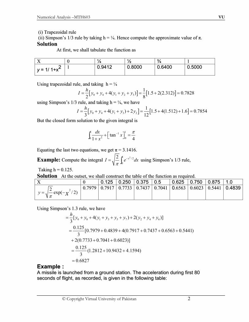
Numerical Analysis –MTH603 VU
© Copyright Virtual University of Pakistan 2
((ii)) TTrraappeezzooiiddaall rruullee
((iiii)) SSiimmppssoonn’’ss 11//33 rruullee bbyy ttaakkiinngg hh == ¼¼.. HHeennccee ccoommppuuttee tthhee aapppprrooxxiimmaattee vvaalluuee ooff ..
SSoolluuttiioonn
AAtt ffiirrsstt,, wwee sshhaallll ttaabbuullaattee tthhee ffuunnccttiioonn aass
XX 00 ¼¼ ½½ ¾¾ 11
yy == 11// 11++xx22
11 00..99441122 00..88000000 00..66440000 00..55000000
UUssiinngg ttrraappeezzooiiddaall rruullee,, aanndd ttaakkiinngg hh == ¼¼
( ) ( )0 4 1 2 3
14( ) 1.5 2(2.312) 0.7828
2 8
hI y y y y y! " " " " ! " !
uussiinngg SSiimmppssoonn’’ss 11//33 rruullee,, aanndd ttaakkiinngg hh == ¼¼,, wwee hhaavvee
( ) ( )0 4 1 3 2
14( ) 2 1.5 4(1.512) 1.6 0.7854
3 12
hI y y y y y! " " " " ! " " !
BBuutt tthhee cclloosseedd ffoorrmm ssoolluuttiioonn ttoo tthhee ggiivveenn iinntteeggrraall iiss
1 1
1
2 00tan
1 4
dxx
x
*$+ ," !- ."
EEqquuaattiinngg tthhee llaasstt ttwwoo eeqquuaattiioonnss,, wwee ggeett == 33..11441166..
EExxaammppllee:: CCoommppuuttee tthhee iinntteeggrraall 21
/ 2
0
2 xI e dx*
$! uussiinngg SSiimmppssoonn’’ss 11//33 rruullee,,
TTaakkiinngg hh == 00..112255..
SSoolluuttiioonn AAtt tthhee oouuttsseett,, wwee sshhaallll ccoonnssttrruucctt tthhee ttaabbllee ooff tthhee ffuunnccttiioonn aass rreeqquuiirreedd..
XX 00 00..112255 00..225500 00..337755 00..55 00..662255 00..775500 00..887755 11..00
22exp( / 2)y x*
! $ 00..77997799
00..77991177 00..77773333 00..77443377
00..77004411 00..66556633 00..66002233 00..55444411 00..44883399
UUssiinngg SSiimmppssoonn’’ss 11..33 rruullee,, wwee hhaavvee
0 8 1 3 5 7 2 4 6[ 4( ) 2( )]
3
0.125[0.7979 0.4839 4(0.7917 0.7437 0.6563 0.5441)
3
hy y y y y y y y y! " " " " " " " "
! " " " " "
2(0.7733 0.7041 0.6023)]
0.125(1.2812 10.9432 4.1594)
3
0.6827
" " "
! " "
!
EExxaammppllee ::
AA mmiissssiillee iiss llaauunncchheedd ffrroomm aa ggrroouunndd ssttaattiioonn.. TThhee aacccceelleerraattiioonn dduurriinngg ffiirrsstt 8800
sseeccoonnddss ooff fflliigghhtt,, aass rreeccoorrddeedd,, iiss ggiivveenn iinn tthhee ffoolllloowwiinngg ttaabbllee::

Numerical Analysis –MTH603 VU
© Copyright Virtual University of Pakistan 3
( )t s 00 1100 2200 3300 4400 5500 6600 7700 8800 2( / )a m s 3300..0000
3311..6633 3333..3344 3355..4477 3377..7755 4400..3333 4433..2255 4466..6699 5500..6677
CCoommppuuttee tthhee vveelloocciittyy ooff tthhee mmiissssiillee wwhheenn tt == 8800 ss,, uussiinngg SSiimmppssoonn’’ss 11//33 rruullee..
SSoolluuttiioonn::
SSiinnccee aacccceelleerraattiioonn iiss ddeeffiinneedd aass tthhee rraattee ooff cchhaannggee ooff vveelloocciittyy,, wwee hhaavvee
80
0v a dt ! Or
dva
dt
UUssiinngg SSiimmppssoonn’’ss 11//33--rruullee,, wwee hhaavvee
0 8 1 3 7 2 4 6[( ) 4( ) 2( )]3
10[(30 50.67) 4(31.63 35.47 40.33 46.69) 2(33.34 37.75 43.25)]
3
3086.1 /
hv y y y y y y y y
m s
" " " " " " "
" " " " " " " "
TThheerreeffoorree,, tthhee rreeqquuiirreedd vveelloocciittyy iiss ggiivveenn bbyy yy == 33..00886611 kkmm//ss..

Numerical Analysis –MTH603 VU
© Copyright Virtual University of Pakistan 1
SSiimmppssoonn’’ss 33//88 rruullee
CCoonnssiiddeerr tthhee ddeeffiinniittee iinntteeggrraall ( )b
x aI f x dx
!
1
0
3
0 0 1 1 0 1( ) Error ( ) ( )2 12
x
x
h hf x dx c y c y y y y "## $ $ $ %!
TThheenn,, iiff nn == 22,, tthhee iinntteeggrraattiioonn ttaakkeess tthhee ffoorrmm
2
00 0 1 1 2 2
5( )
0 1 2
( ) Error
( 4 ) ( )3 90
x
x
iv
f x dx x y x y x y
h hy y y y "
$ $ $
$ $ %
!
TThhuuss SSiimmppssoonn’’ss 11//33 rruullee iiss bbaasseedd oonn ffiittttiinngg tthhrreeee ppooiinnttss wwiitthh aa qquuaaddrraattiicc..
SSiimmiillaarrllyy,, ffoorr nn == 33,, tthhee iinntteeggrraattiioonn iiss ffoouunndd ttoo bbee
3
0
5 ( )
0 1 2 3
3 3( ) ( 3 3 ) h ( )
8 80
xiv
xf x dx h y y y y y " $ $ $ %!
TThhiiss iiss kknnoowwnn aass SSiimmppssoonn’’ss 33//88 rruullee,, wwhhiicchh iiss bbaasseedd oonn ffiittttiinngg ffoouurr ppooiinnttss bbyy aa ccuubbiicc..
SSttiillll hhiigghheerr oorrddeerr NNeewwttoonn--CCootteess iinntteeggrraattiioonn ffoorrmmuullaaee ccaann bbee ddeerriivveedd ffoorr llaarrggee vvaalluueess ooff nn..
TTRRAAPPEEZZOOIIDDAALL RRUULLEE
0
0 1 2 1( ) ( 2 2 2 )2
nx
n n nx
hf x dx y y y y y E% $ $ $ $ $ $!
0
0 1 2 1( ) ( 2 2 2 )2
nx
n n nx
hf x dx y y y y y E% $ $ $ $ $ $!
SSIIMMPPSSOONN’’SS 11//33 RRUULLEE
2
0
5( )
0 1 2( ) ( 4 ) ( )3 90
xiv
x
h hI f x dx y y y y " $ $ %!
2
00 1 3 2 1 2 4 2 2 2( ) [ 4( ) 2( ) ] Error term
3
Nx
N N Nx
hf x dx y y y y y y y y% % $ $ $ $ $ $ $ $ $ $!
4 ( )2 0 ( )180
ivNx xE h y "
% %
SSiimmppssoonn’’ss 33//88 rruullee iiss
1 2 3 4 5 6 3 2 1
3( ) [ ( ) 3 3 2 3 3 2 2 3 3 ( )]
8
b
n n na
f x dx h y a y y y y y y y y y y b% % % $ $ $ $ $ $ $ $ $ $ $!
WWiitthh tthhee gglloobbaall eerrrroorr EE ggiivveenn bbyy
4 ( )0 ( )80
ivnx xE h y "
% %
RROOMMBBEERRGG’’SS IINNTTEEGGRRAATTIIOONN
WWee hhaavvee oobbsseerrvveedd tthhaatt tthhee ttrraappeezzooiiddaall rruullee ooff iinntteeggrraattiioonn ooff aa ddeeffiinniittee iinntteeggrraall iiss ooff
OO((hh22)),, wwhhiillee tthhaatt ooff SSiimmppssoonn’’ss 11//33 aanndd 33//88 rruulleess aarree ooff ffoouurrtthh--oorrddeerr aaccccuurraattee..

Numerical Analysis –MTH603 VU
© Copyright Virtual University of Pakistan 2
WWee ccaann iimmpprroovvee tthhee aaccccuurraaccyy ooff ttrraappeezzooiiddaall aanndd SSiimmppssoonn’’ss rruulleess uussiinngg RRiicchhaarrddssoonn’’ss
eexxttrraappoollaattiioonn pprroocceedduurree wwhhiicchh iiss aallssoo ccaalllleedd RRoommbbeerrgg’’ss iinntteeggrraattiioonn mmeetthhoodd..
FFoorr eexxaammppllee,, tthhee eerrrroorr iinn ttrraappeezzooiiddaall rruullee ooff aa ddeeffiinniittee iinntteeggrraall
( )b
aI f x dx !
ccaann bbee wwrriitttteenn iinn tthhee ffoorrmm
2 4 6
1 2 3TI I c h c h c h $ $ $ $
BByy aappppllyyiinngg RRiicchhaarrddssoonn’’ss eexxttrraappoollaattiioonn pprroocceedduurree ttoo ttrraappeezzooiiddaall rruullee,, wwee oobbttaaiinn tthhee
ffoolllloowwiinngg ggeenneerraall ffoorrmmuullaa
( 1) ( 1) 1
1
42 2
2 4
m
T m T mm m
Tm m m
h hI I
hI
% % %
%
& ' & '%( ) ( )& ' * + * + ( )* +
WWhheerree mm == 11,, 22,, …… ,, wwiitthh
IITT00
((hh)) == IITT
((hh))..
FFoorr iilllluussttrraattiioonn,, wwee ccoonnssiiddeerr tthhee ffoolllloowwiinngg eexxaammppllee..
Example:
UUssiinngg RRoommbbeerrgg’’ss iinntteeggrraattiioonn mmeetthhoodd,, ffiinndd tthhee vvaalluuee ooff 1.8
1( )y x dx! ssttaarrttiinngg wwiitthh
ttrraappeezzooiiddaall rruullee,, ffoorr tthhee ttaabbuullaarr vvaalluueess
x 1.0 1.1 1.2 1.3 1.4 1.5 1.6 1.7 1.8
y = f(x) 1.543 1.669 1.811 1.971 2.151 2.352 2.577 2.828 3.107
Solution:
0
0
1, 1.8,
1.8 1.0,
n
i
x x
h x x ihN
% $
LLeett IITT
ddeennoottee tthhee iinntteeggrraattiioonn bbyy TTrraappeezzooiiddaall rruullee,, tthheenn ffoorr
0 11, 0.8, ( )2
0.4(1.543 3.107) 1.8600
T
hN h I y y $
$
0 1 22, 0.4, ( 2 ) 0.2[1.543 2(2.151) 3.107]2
1.7904
T
hN h I y y y $ $ $ $
0 1 2 3 44, 0.2, [ 2( ) ] 0.1[1.543 2(1.811 2.151 2.577) 3.107]2
1.7728
T
hN h I y y y y y $ $ $ $ $ $ $ $
Similarly for

Numerical Analysis –MTH603 VU
© Copyright Virtual University of Pakistan 3
8, 0.1,
1.7684T
N h
I
Now, using Romberg’s formula , we have
1
4(1.7904) 1.8600
2 3
1.7672
T
hI
%& ' ( )* +
2
2 2 2
4 (1.7728) 1.7672
2 4 1
1.77317
T
hI
%& ' ( ) %* +
3
3 3 3
4 (1.7672) 1.77317
2 4 1
1.7671
T
hI
%& ' ( ) %* +
Thus, after three steps, it is found that the value of the tabulated integral is 1.7671.
DDOOUUBBLLEE IINNTTEEGGRRAATTIIOONN TToo eevvaalluuaattee nnuummeerriiccaallllyy aa ddoouubbllee iinntteeggrraall ooff tthhee ffoorrmm
( , )I x y dx dy, - . /! !
oovveerr aa rreeccttaanngguullaarr rreeggiioonn bboouunnddeedd bbyy tthhee lliinneess xx == aa,, xx ==bb,, yy == cc,, yy == dd wwee sshhaallll eemmppllooyy
eeiitthheerr ttrraappeezzooiiddaall rruullee oorr SSiimmppssoonn’’ss rruullee,, rreeppeeaatteeddllyy WWiitthh rreessppeecctt ttoo oonnee vvaarriiaabbllee aatt
aa ttiimmee.. NNoottiinngg tthhaatt,, bbootthh tthhee iinntteeggrraattiioonnss aarree jjuusstt aa lliinneeaarr ccoommbbiinnaattiioonn ooff vvaalluueess ooff tthhee
ggiivveenn ffuunnccttiioonn aatt ddiiffffeerreenntt vvaalluueess ooff tthhee iinnddeeppeennddeenntt vvaarriiaabbllee,, wwee ddiivviiddee tthhee iinntteerrvvaall [[aa,, bb]]
iinnttoo NN eeqquuaall ssuubb--iinntteerrvvaallss ooff ssiizzee hh,, ssuucchh tthhaatt hh == ((bb –– aa))//NN;; aanndd tthhee iinntteerrvvaall ((cc,, dd)) iinnttoo MM
eeqquuaall ssuubb--iinntteerrvvaallss ooff ssiizzee kk,, ssoo tthhaatt kk == ((dd –– cc))//MM.. TThhuuss,, wwee hhaavvee
0 0, ,ix x ih x a $
0 0
, for 1, 2,..., 1
, ,
, for 1, 2,..., 1
N
i
M
x b i N
y y ik y c
y d i M
%
$
%
TThhuuss,, wwee ccaann ggeenneerraattee aa ttaabbllee ooff vvaalluueess ooff tthhee iinntteeggrraanndd,, aanndd tthhee aabboovvee pprroocceedduurree ooff
iinntteeggrraattiioonn iiss iilllluussttrraatteedd bbyy ccoonnssiiddeerriinngg aa ccoouuppllee ooff eexxaammpplleess..
EExxaammppllee EEvvaalluuaattee tthhee ddoouubbllee iinntteeggrraall
2 2
1 1
dxdyI
x y
$! !
bbyy uussiinngg ttrraappeezzooiiddaall rruullee,, wwiitthh hh == kk == 00..2255..
SSoolluuttiioonn

Numerical Analysis –MTH603 VU
© Copyright Virtual University of Pakistan 4
TTaakkiinngg xx == 11,, 11..2255,, 11..5500,, 11..7755,, 22..00 aanndd yy == 11,, 11..2255,, 11..5500,, 11..7755,, 22..00,, tthhee ffoolllloowwiinngg ttaabbllee iiss
ggeenneerraatteedd uussiinngg tthhee iinntteeggrraanndd
1
( , )f x yx y
$
x y
1.00 1.25 1.50 1.75 2.00
1.00 0.5 0.4444 0.4 0.3636 0.3333
1.25 0.4444 0.4 0.3636 0.3333 0.3077
1.50 0.4 0.3636 0.3333 0.3077 0.2857
1.75 0.3636 0.3333 0.307 0.2857 0.2667
2.00 0.3333 0.3077 0.2857 0.2667 0.25
KKeeeeppiinngg oonnee vvaarriiaabbllee ssaayy xx ffiixxeedd aanndd vvaarryyiinngg tthhee vvaarriiaabbllee yy,, tthhee aapppplliiccaattiioonn ooff
ttrraappeezzooiiddaall rruullee ttoo eeaacchh rrooww iinn tthhee aabboovvee ttaabbllee ggiivveess 2
1
0.25(1, ) [0.5 2(0.4444 0.4 0.3636) 0.3333]
2
0.4062
f y dy $ $ $ $
!
2
1
0.25(1.25, ) [0.4444 2(0.4 0.3636 0.3333) 0.3077]
2
0.3682
f y dy $ $ $ $
!
2
1
0.25(1.5, ) [0.4 2(0.3636 0.3333 0.3077)] 0.2857
2
0.3369
f y dy $ $ $ $
!
2
1
0.25(1.75, ) [0.3636 2(0.3333 0.3077 0.2857) 0.2667]
2
0.3105
f y dy $ $ $ $
!
and
2
1
0.25(2, ) [0.3333 2(0.3077 0.2857) 0.25]
2
0.2879
f y dy $ $ $
!
Therefore

Numerical Analysis –MTH603 VU
© Copyright Virtual University of Pakistan 5
0 12 2
1 1(1, ) 2[ (1.25, ) (1.5, ) (1.75, )] (2, )
2
dxdy hI f y f y f y f y f y
x y $ $ $ $
$! !
BByy uussee ooff tthhee llaasstt eeqquuaattiioonnss wwee ggeett tthhee rreeqquuiirreedd rreessuulltt aass
2 30.25.04602 2(0.3682 0.3369 0.3105) 0.2879 0.3407
2I $ $ $ $
EExxaammppllee ::EEvvaalluuaattee
/ 2 / 2
0 0sin( )x y dxdy
4 4$! !
bbyy nnuummeerriiccaall ddoouubbllee iinntteeggrraattiioonn..
SSoolluuttiioonn TTaakkiinngg xx == yy == //44,, 33 //88,, //22,, wwee ccaann ggeenneerraattee tthhee ffoolllloowwiinngg ttaabbllee ooff tthhee iinntteeggrraanndd
( , ) sin( )f x y x y $
x y
0 /8 /4 3 /8 /2
0 0.0 0.6186 0.8409 0.9612 1.0
/8 0.6186 0.8409 0.9612 1.0 0.9612
/4 0.8409 0.9612 1.0 0.9612 0.8409
3 /8 0.9612 1.0 0.9612 0.8409 0.6186
/2 1.0 0.9612 0.8409 0.6186 0.0
KKeeeeppiinngg oonnee vvaarriiaabbllee aass ssaayy xx ffiixxeedd aanndd yy aass vvaarriiaabbllee,, aanndd aappppllyyiinngg ttrraappeezzooiiddaall rruullee ttoo
eeaacchh rrooww ooff tthhee aabboovvee ttaabbllee,, wwee ggeett
2 3/ 2
0(0, ) 0.0 2(0.6186 0.8409 0.9612) 1.0 1.1469
16f y dx
4 4 $ $ $ $ !
2 32
0, 0.6186 2(0.8409 0.9612 1.0) 0.9612 1.4106
8 16y dx
4 4 4& ' $ $ $ $ ( )* +!
Similarly we get

Numerical Analysis –MTH603 VU
© Copyright Virtual University of Pakistan 6
2
0
2
0
, 1.4778,4
3, 1.4106
8
f y dx
f y dx
4
4
4
4
& ' ( )* +
& ' ( )* +
!
!
and
2
0, 1.1469
2f y dx
4 4& ' ( )* +!
UUssiinngg tthheessee rreessuullttss,, wwee ffiinnaallllyy oobbttaaiinn
2 2
0 0
3sin( ) (0, ) 2 , , , ,
16 8 4 8 2x y dxdy f y y f y f y f y
4 4 4 4 4 4 45 6& ' & ' & ' & '$ $ $ $ $7 8( ) ( ) ( ) ( )* + * + * + * +9 :
! !
2 31.1469 2(1.4106 1.4778 1.4106) 1.146916
2.1386
4 $ $ $ $

Numerical Analysis –MTH603 VU
© Copyright Virtual University of Pakistan 1
Ordinary Differential Equations IInnttrroodduuccttiioonn
TTaayylloorr SSeerriieess
EEuulleerr MMeetthhoodd
RRuunnggee--KKuuttttaa MMeetthhoodd
PPrreeddiiccttoorr CCoorrrreeccttoorr MMeetthhoodd
IInnttrroodduuccttiioonn
MMaannyy pprroobblleemmss iinn sscciieennccee aanndd eennggiinneeeerriinngg wwhheenn ffoorrmmuullaatteedd mmaatthheemmaattiiccaallllyy aarree rreeaaddiillyy
eexxpprreesssseedd iinn tteerrmmss ooff oorrddiinnaarryy ddiiffffeerreennttiiaall eeqquuaattiioonnss ((OODDEE)) wwiitthh iinniittiiaall aanndd bboouunnddaarryy
ccoonnddiittiioonn..
EExxaammppllee TThhee ttrraajjeeccttoorryy ooff aa bbaalllliissttiicc mmiissssiillee,, tthhee mmoottiioonn ooff aann aarrttiiffiicciiaall ssaatteelllliittee iinn iittss oorrbbiitt,, aarree
ggoovveerrnneedd bbyy oorrddiinnaarryy ddiiffffeerreennttiiaall eeqquuaattiioonnss..
TThheeoorriieess ccoonncceerrnniinngg eelleeccttrriiccaall nneettwwoorrkkss,, bbeennddiinngg ooff bbeeaammss,, ssttaabbiilliittyy ooff aaiirrccrraafftt,, eettcc..,, aarree
mmooddeelleedd bbyy ddiiffffeerreennttiiaall eeqquuaattiioonnss..
TToo bbee mmoorree pprreecciissee,, tthhee rraattee ooff cchhaannggee ooff aannyy qquuaannttiittyy wwiitthh rreessppeecctt ttoo aannootthheerr ccaann bbee
mmooddeelleedd bbyy aann OODDEE
CClloosseedd ffoorrmm ssoolluuttiioonnss mmaayy nnoott bbee ppoossssiibbllee ttoo oobbttaaiinn,, ffoorr eevveerryy mmooddeelleedd pprroobblleemm,, wwhhiillee
nnuummeerriiccaall mmeetthhooddss eexxiisstt,, ttoo ssoollvvee tthheemm uussiinngg ccoommppuutteerrss..
IInn ggeenneerraall,, aa lliinneeaarr oorr nnoonn--lliinneeaarr oorrddiinnaarryy ddiiffffeerreennttiiaall eeqquuaattiioonn ccaann bbee wwrriitttteenn aass
1
1, , , ,
n n
n n
d y dy d yf t y
dt dt dt
! "# $ %
& '
HHeerree wwee sshhaallll ffooccuuss oonn aa ssyysstteemm ooff ffiirrsstt oorrddeerr
ddiiffffeerreennttiiaall eeqquuaattiioonnss ooff tthhee ffoorrmm ( , )dy
f t ydt
# wwiitthh tthhee iinniittiiaall ccoonnddiittiioonn yy ((tt00)) == yy
00,,
wwhhiicchh iiss ccaalllleedd aann iinniittiiaall vvaalluuee pprroobblleemm ((IIVVPP))..
IItt iiss jjuussttiiffiieedd,, iinn vviieeww ooff tthhee ffaacctt tthhaatt aannyy hhiigghheerr oorrddeerr OODDEE ccaann bbee rreedduucceedd ttoo aa ssyysstteemm ooff
ffiirrsstt oorrddeerr ddiiffffeerreennttiiaall eeqquuaattiioonnss bbyy ssuubbssttiittuuttiioonn..
FFoorr eexxaammppllee,, ccoonnssiiddeerr aa sseeccoonndd oorrddeerr ddiiffffeerreennttiiaall eeqquuaattiioonn ooff tthhee ffoorrmm
( , , )y f t y y(( (#
IInnttrroodduucciinngg tthhee ssuubbssttiittuuttiioonn ,p y(# tthhee aabboovvee eeqquuaattiioonn rreedduucceess ttoo aa ssyysstteemm ooff ttwwoo ffiirrsstt
oorrddeerr ddiiffffeerreennttiiaall eeqquuaattiioonnss,, ssuucchh aass
, ( , , )y p p f t y p( (# #
TThheeoorreemm
LLeett ff ((tt,, yy)) bbee rreeaall aanndd ccoonnttiinnuuoouuss iinn tthhee ssttrriipp RR,, ddeeffiinneedd bbyy ) *0 , ,t t T y+ , - - ,
TThheenn ffoorr aannyy 0[ , ]t t T+ aanndd ffoorr aannyy yy11,, yy
22,, tthheerree eexxiissttss aa ccoonnssttaanntt LL,, ssaattiissffyyiinngg tthhee
iinneeqquuaalliittyy 1 2 1 2( , ) ( , )f t y f t y L y y - ssoo tthhaatt ( , ) ,yf t y L- ffoorr eevveerryy ,t y R+
HHeerree,, LL iiss ccaalllleedd LLiippsscchhiittzz ccoonnssttaanntt..

Numerical Analysis –MTH603 VU
© Copyright Virtual University of Pakistan 2
IIff tthhee aabboovvee ccoonnddiittiioonnss aarree ssaattiissffiieedd,, tthheenn ffoorr aannyy yy00,, tthhee IIVVPP hhaass aa uunniiqquuee ssoolluuttiioonn yy (( tt )),,
ffoorr ) *0 ,t t T+
IInn ffaacctt,, wwee aassssuummee tthhee eexxiisstteennccee aanndd uunniiqquueenneessss ooff tthhee ssoolluuttiioonn ttoo tthhee aabboovvee IIVVPP
TThhee ffuunnccttiioonn mmaayy bbee lliinneeaarr oorr nnoonn--lliinneeaarr.. WWee aallssoo aassssuummee tthhaatt tthhee ffuunnccttiioonn ff ((tt,, yy)) iiss
ssuuffffiicciieennttllyy ddiiffffeerreennttiiaabbllee wwiitthh rreessppeecctt ttoo eeiitthheerr tt oorr yy..
TTAAYYLLOORR’’SS SSEERRIIEESS
MMEETTHHOODD CCoonnssiiddeerr aann iinniittiiaall vvaalluuee pprroobblleemm ddeessccrriibbeedd bbyy
0 0( , ), ( )dy
f t y y t ydt
# #
HHeerree,, wwee aassssuummee tthhaatt ff ((tt,, yy)) iiss ssuuffffiicciieennttllyy ddiiffffeerreennttiiaabbllee wwiitthh rreessppeecctt ttoo xx aanndd yy..
IIff yy ((tt)) iiss tthhee eexxaacctt ssoolluuttiioonn,, wwee ccaann eexxppaanndd yy ((tt)) bbyy TTaayylloorr’’ss sseerriieess aabboouutt tthhee ppooiinntt tt == tt00
aanndd oobbttaaiinn 2
00 0 0 0
( )( ) ( ) ( ) ( ) ( )
2!
t ty t y t t t y t y t
( ((# . .
3 4
0 00 0
( ) ( )( ) ( )
3! 4!
IVt t t ty t y t
(((. . .
SSiinnccee,, tthhee ssoolluuttiioonn iiss nnoott kknnoowwnn,, tthhee ddeerriivvaattiivveess iinn tthhee aabboovvee eexxppaannssiioonn aarree nnoott kknnoowwnn
eexxpplliicciittllyy.. HHoowweevveerr,, ff iiss aassssuummeedd ttoo bbee ssuuffffiicciieennttllyy ddiiffffeerreennttiiaabbllee aanndd tthheerreeffoorree,, tthhee
ddeerriivvaattiivveess ccaann bbee oobbttaaiinneedd ddiirreeccttllyy ffrroomm tthhee ggiivveenn ddiiffffeerreennttiiaall eeqquuaattiioonn..
NNoottiinngg tthhaatt ff iiss aann iimmpplliicciitt ffuunnccttiioonn ooff yy,, wwee hhaavvee
( , )
x y
y f t y
f f dyy f ff
x y dx
( # /0
1 1 2(( # . # . 01 1 3
Similarly
2
2
2
2
( ) ( )
2 ( )
3 3
( 2 )
3( )( )
( )
xx xy xy yy y x y
xx xy yy y x y
IV
xxx xxx xyy
y xx xy yy
x y xy yy
y x y
y f ff f f ff f f ff
f ff f f f f ff
y f ff f f
f f ff f f
f ff ff ff
f f ff
((( # . . . . . /0
# . . . . 00
# . . 02
. . . 00. . . 00. . 3
CCoonnttiinnuuiinngg iinn tthhiiss mmaannnneerr,, wwee ccaann eexxpprreessss aannyy ddeerriivvaattiivvee ooff yy iinn tteerrmmss ooff
ff ((tt,, yy)) aanndd iittss ppaarrttiiaall ddeerriivvaattiivveess..
EExxaammppllee UUssiinngg TTaayylloorr’’ss sseerriieess mmeetthhoodd,, ffiinndd tthhee ssoolluuttiioonn ooff tthhee iinniittiiaall vvaalluuee pprroobblleemm
, (1) 0dy
t y ydt
# . #
aatt tt == 11..22,, wwiitthh hh == 00..11 aanndd ccoommppaarree tthhee rreessuulltt wwiitthh tthhee cclloosseedd ffoorrmm ssoolluuttiioonn
SSoolluuttiioonn LLeett uuss ccoommppuuttee tthhee ffiirrsstt ffeeww ddeerriivvaattiivveess ffrroomm tthhee ggiivveenn ddiiffffeerreennttiiaall eeqquuaattiioonn aass ffoolllloowwss::

Numerical Analysis –MTH603 VU
© Copyright Virtual University of Pakistan 3
, 1 , ,
,IV V IV
y t y y y y y
y y y y
( (( ( ((( ((# . # . #
(((# #
PPrreessccrriibbiinngg tthhee iinniittiiaall ccoonnddiittiioonn,, tthhaatt iiss,, aatt
tt00 ==11,, yy
00 –– yy ((tt
00)) == 00,, wwee hhaavvee
0 0
0 0 0
1, 2,
2IV V
y y
y y y
( ((# #
(((# # #
NNooww,, uussiinngg TTaayylloorr’’ss sseerriieess mmeetthhoodd,, wwee hhaavvee
2 3
0 00 0 0 0 0
4 5
0 00 0
( ) ( )( ) ( )
2 6
( ) ( )
24 120
IV V
t t t ty t y t t y y y
t t t ty y
( (( (((# . . .
. . .
SSuubbssttiittuuttiinngg tthhee aabboovvee vvaalluueess ooff tthhee ddeerriivvaattiivveess,, aanndd tthhee iinniittiiaall ccoonnddiittiioonn,, wwee oobbttaaiinn
0.01 0.001 0.00001
(1.1) 0 (0.1)(1) (2) (2) (2)2 6 120
y # . . . . .
0.001 0.0001 0.00001
0.1 0.013 12 60
# . . . . .
0.1 0.01 0.000333 0.0000083 0.0000001# . . . . .
0.1103414#
Therefore
1(1.1) 0.1103414 0.1103y y# # 4
TTaakkiinngg yy11 == 00..11110033 aatt tt == 11..11,, tthhee vvaalluueess ooff tthhee ddeerriivvaattiivveess aarree
1
1
1 1 1
1.1 0.1103 1.2103
1 1.2103 2.2103
2.2103IV V
y
y
y y y
( # . #
((# . #
(((# # #
SSuubbssttiittuuttiinngg tthhee vvaalluuee ooff yy11 aanndd iittss ddeerriivvaattiivveess iinnttoo TTaayylloorr’’ss sseerriieess eexxppaannssiioonn wwee ggeett,,
aafftteerr rreettaaiinniinngg tteerrmmss uupp ttoo ffiifftthh ddeerriivvaattiivvee oonnllyy…………
2
11 1 1 1
3 4 5
1 1 11 1 1
( )(1.2) ( )
2
( ) ( ) ( )
6 24 120
IV V
t ty y t t y y
t t t t t ty y y
( ((# . .
(((. . .
(1.2) 0.1103 0.12103
0.0110515 0.0003683
0.000184 0.0000003
y # .
. .
. .
0.2429341 0.2429 0.243# 5!
TToo oobbttaaiinn tthhee cclloosseedd ffoorrmm ssoolluuttiioonn,, wwee rreewwrriittee tthhee ggiivveenn IIVVPP aass
dy
y tdt
# or ( )t td ye te #
OOnn iinntteeggrraattiioonn,, wwee ggeett

Numerical Analysis –MTH603 VU
© Copyright Virtual University of Pakistan 4
( )
1
t t t t
t
y e te e ce
ce t
# . .
#
UUssiinngg tthhee iinniittiiaall ccoonnddiittiioonn,, wwee ggeett TThheerreeffoorree,, tthhee cclloosseedd ffoorrmm ssoolluuttiioonn iiss
11 2 ty t e # .
WWhheenn tt == 11..22,, tthhee cclloosseedd ffoorrmm ssoolluuttiioonn bbeeccoommeess
(1.2) 1.2 1 2(1.2214028)
2.2 2.4428056
0.2428 0.243
y # .
.
# 5
Example Using Taylor’s Series method taking algorithm of order 3, solve the initial value problem
/ 1 ; (0) 0 0.25y y y with h# # # at x= .50
Solution:

Numerical Analysis –MTH603 VU
© Copyright Virtual University of Pakistan 5
6 7
6 7
6 7 6 7 6 7 6 7
/ / / / / / / / /
0 0
/
/ / /
/ / / / /
2 3
1 0 1 0/ / /
1 0 1 0 0 0 0
1
0 0 ,
1 0 1
1
1 1
, ' lg
2 3 !
L e t u s c o m p u te th e f i r s t th r e e d e r iv a t iv e s
y y y y y y
T h e in i t ia l c o n d i t io n i s
t y w e h a v e
y
y y
y y
N o w T a y lo r s s e r ie s m e th o s d a r i th m is
t t t ty t y t t y y y
# # #
# #
# #
# #
# # #
# . . .
6 7 6 76 7 6 7 6 7 6 7 6 7
6 7
6 76 7
6 7
/ / /
/ 2 / / 3 / / /
1 0 0 0 0
2 3
1
/
/ / /
1 1( ) 0 .2 5
2 3 !
0 .2 5 0 .2 50 .2 5 0 0 .2 5 1 1 1
2 3 !
0 .0 6 2 5 0 .0 1 5 6 2 50 .2 5 0 .2 5
2 6
0 .2 5 0 .2 5 0 .0 3 1 2 5 0 .0 0 2 6 0 4 1 6 7
0 .2 5 0 .2 2 1 3 5
0 .2 2 1 3 5 ,
1 1 0 .2 2 1 3 5 0 .7 7 8 6
0 .
O R y t y h y h y h y h
y
y
y
y
T a k in g y N o w
y y
y y
# . . . #
# . . .
# .
# .
#
#
# # #
# #
6 7/ / / / /
7 7 8 6
0 .7 7 8 6 0 .7 7 8 6y y# # #
6 7 6 7 6 7 6 7
6 7
2 3
2 1 2 1/ // ///
2 1 2 1 1 1 1
/ 2 // 3 ///
2 1 1 1 1
2 3
2 3!
1 1.25
2 6
1 10.22135 (0.25)(0.7786) (0.25) ( 0.7786) (0.25) (0.7786)
2 6
0.22135 0.19465 0.02433 0.002027
0.39369
t t t ty t y t t y y y
OR y t y hy h y h y h
# . . .
# . . . #
# . . .
# . .
#

Numerical Analysis –MTH603 VU
© Copyright Virtual University of Pakistan 1
EEUULLEERR MMEETTHHOODD EEuulleerr mmeetthhoodd iiss oonnee ooff tthhee oollddeesstt nnuummeerriiccaall mmeetthhooddss uusseedd ffoorr iinntteeggrraattiinngg tthhee oorrddiinnaarryy
ddiiffffeerreennttiiaall eeqquuaattiioonnss.. TThhoouugghh tthhiiss mmeetthhoodd iiss nnoott uusseedd iinn pprraaccttiiccee,, iittss uunnddeerrssttaannddiinngg wwiillll
hheellpp uuss ttoo ggaaiinn iinnssiigghhtt iinnttoo nnaattuurree ooff pprreeddiiccttoorr--ccoorrrreeccttoorr mmeetthhoodd
CCoonnssiiddeerr tthhee ddiiffffeerreennttiiaall eeqquuaattiioonn ooff ffiirrsstt oorrddeerr wwiitthh tthhee iinniittiiaall ccoonnddiittiioonn yy((tt00
)) == yy00
..
( , )dy
f t ydt
TThhee iinntteeggrraall ooff tthhiiss eeqquuaattiioonn iiss aa ccuurrvvee iinn,, ttyy--ppllaannee..
HHeerree,, wwee ffiinndd ssuucccceessssiivveellyy yy11,, yy
22,, ……,, yy
mm;; wwhheerree yy
mm iiss tthhee vvaalluuee ooff yy aatt tt ==tt
mm == tt
00 ++mmhh,,
mm ==11,, 22,,…… aanndd hh bbeeiinngg ssmmaallll..
HHeerree wwee uussee aa pprrooppeerrttyy tthhaatt iinn aa ssmmaallll iinntteerrvvaall,, aa ccuurrvvee iiss nneeaarrllyy aa ssttrraaiigghhtt lliinnee.. TThhuuss aatt
((tt00,, yy
00)),, wwee aapppprrooxxiimmaattee tthhee ccuurrvvee bbyy aa ttaannggeenntt aatt tthhaatt ppooiinntt..
TThheerreeffoorree,,
0 0
00 0
( , ) 0
( , )t y
y ydyf t y
dt t t
!" # $ % !& '
That is 0 0 0 0( ) ( , )y y t t f t y ( !
HHeennccee,, tthhee vvaalluuee ooff yy ccoorrrreessppoonnddiinngg ttoo tt == tt11 iiss ggiivveenn bbyy
1 0 1 0 0 0( ) ( , )y y t t f t y ( !
SSiimmiillaarrllyy aapppprrooxxiimmaattiinngg tthhee ssoolluuttiioonn ccuurrvvee iinn tthhee nneexxtt iinntteerrvvaall ((tt11,, tt
22)) bbyy aa lliinnee tthhrroouugghh
((tt11,, yy
11)) hhaavviinngg iittss ssllooppee ff((tt
11,, yy
11)),, wwee oobbttaaiinn
2 1 1 1( , )y y hf t y (
TThhuuss,, wwee oobbttaaiinn iinn ggeenneerraall,, tthhee ssoolluuttiioonn ooff tthhee ggiivveenn ddiiffffeerreennttiiaall eeqquuaattiioonn iinn tthhee ffoorrmm ooff aa
rreeccuurrrreennccee rreellaattiioonn
1 ( , )m m m my y hf t y( (
GGeeoommeettrriiccaallllyy,, tthhiiss mmeetthhoodd hhaass aa vveerryy ssiimmppllee mmeeaanniinngg.. TThhee ddeessiirreedd ffuunnccttiioonn ccuurrvvee iiss
aapppprrooxxiimmaatteedd bbyy aa ppoollyyggoonn ttrraaiinn,, wwhheerree tthhee ddiirreeccttiioonn ooff eeaacchh ppaarrtt iiss ddeetteerrmmiinneedd bbyy tthhee
vvaalluuee ooff tthhee ffuunnccttiioonn ff ((tt,, yy)) aatt iittss ssttaarrttiinngg ppooiinntt..
EExxaammppllee
GGiivveenn dy y t
dt y t
!
( wwiitthh tthhee iinniittiiaall ccoonnddiittiioonn yy == 11 aatt tt == 00.. UUssiinngg EEuulleerr mmeetthhoodd,, ffiinndd yy
aapppprrooxxiimmaatteellyy aatt xx == 00..11,, iinn ffiivvee sstteeppss..
SSoolluuttiioonn
SSiinnccee tthhee nnuummbbeerr ooff sstteeppss aarree ffiivvee,, wwee sshhaallll pprroocceeeedd iinn sstteeppss ooff ((00..11))//55 == 00..0022..
TThheerreeffoorree,, ttaakkiinngg sstteepp ssiizzee
hh == 00..0022,, wwee sshhaallll ccoommppuuttee tthhee vvaalluuee ooff yy aatt
tt == 00..0022,, 00..0044,, 00..0066,, 00..0088 aanndd 00..11
Thus 1 0 0 0( , ),y y hf t y ( where 0 01, 0y t

Numerical Analysis –MTH603 VU
© Copyright Virtual University of Pakistan 2
Therefore 1
1 01 0.02 1.02
1 0y
! (
(
Similarly,
2 1 1 1
3 2 2 2
4 3 3 3
5 4 4 4
1.02 0.02( ) 1.02 0.02 1.0392
1.02 0.02
1.0392 0.04( , ) 1.0392 0.02 1.0577
1.0392 0.04
1.0577 0.06( , ) 1.0577 0.02 1.0738
1.0577 0.06
1.0738 0.08( , ) 1.0738 0.02
y y hf t y
y y hf t y
y y hf t y
y y hf t y
! ( ( (
(!
( ( (!
( ( (!
( ( 1.09101.0738 0.08
(
HHeennccee tthhee vvaalluuee ooff yy ccoorrrreessppoonnddiinngg ttoo tt == 00..11 iiss 11..009911
EExxaammppllee Solve the differential equation
/ ; (0) 1y x y y (
in the interval [0,0.5] using Euler’s method by taking h=0.1
Soution:
0 0
1 0 0 0
1
1 1
2 1 1 1
2
0.1 0, 0.1, 0.2, 0.3, 0.4, 0.5
(0) 1 here x 0 1
( , )
1 (0.1)(0 1) 1 0.1 1.1
1.1 0.1
( , )
1.1 (0.1)(0.1 1.1) 1.1 0.12 1.22
Since h so we calculate values at x
y y
y y hf x y
y
y x
y y hf x y
y
) ) )) ) ) ) ) )
) )) ) ))
(
( ( (
))))
(
( ( (
0x 0
1x 0.1
2x 0.2
3x 0.3
4x 0.4
5x 0.5

Numerical Analysis –MTH603 VU
© Copyright Virtual University of Pakistan 3
2 2
3 2 2 2
3
3 3
4 3 3 3
4
4 4
5 4 4 4
1.22 0.2
( , )
1.22 (0.1)(1.22 0.2) 1.22 0.142 1.3620
1.3620 0.3
( , )
1.3620 (0.1)(1.3620 0.3) 1.3620 0.1662 1.5282
1.3620 0.4
( , )
now
y x
y y hf x y
y
now
y x
y y hf x y
y
now
y x
y y hf x y
)
))))
(
( ( (
))))
(
)( ( (
))))
(
5
5 5
6 5 5 5
6
1.5282 (0.1)(1.5282 0.4) 1.7210
1.7210 0.5
( , )
1.7210 (0.1)(1.7210 0.5) 1.9431
0.5 1.9431
y
now
y x
y y hf x y
y
Hencethevalueof y corresponding to t is
)( (
))))
(
)( (
MMOODDIIFFIIEEDD EEUULLEERR’’SS MMEETTHHOODD TThhee mmooddiiffiieedd EEuulleerr’’ss mmeetthhoodd ggiivveess ggrreeaatteerr iimmpprroovveemmeenntt iinn aaccccuurraaccyy oovveerr tthhee oorriiggiinnaall
EEuulleerr’’ss mmeetthhoodd.. HHeerree,, tthhee ccoorree iiddeeaa iiss tthhaatt wwee uussee aa lliinnee tthhrroouugghh ((tt00,, yy
00)) wwhhoossee ssllooppee iiss
tthhee aavveerraaggee ooff tthhee ssllooppeess aatt ((tt00
,,yy00
)) aanndd ((tt11,, yy
11
((11)))) WWhheerree yy
11
((11))== yy
00 ++ hhff ((tt
00,, yy
00)) iiss tthhee
vvaalluuee ooff yy aatt tt == tt11 aass oobbttaaiinneedd iinn EEuulleerr’’ss mmeetthhoodd,, wwhhiicchh aapppprrooxxiimmaatteess tthhee ccuurrvvee iinn tthhee
iinntteerrvvaall ((tt00
,, tt11))

Numerical Analysis –MTH603 VU
© Copyright Virtual University of Pakistan 4
((MMooddiiffiieedd EEuulleerr’’ss MMeetthhoodd))
GGeeoommeettrriiccaallllyy,, ffrroomm FFiigguurree,, iiff LL11 iiss tthhee ttaannggeenntt aatt ((tt
00,, yy
00)),, LL
22 iiss tthhee lliinnee tthhrroouugghh ((tt
11,,
yy11
((11)))) ooff ssllooppee ff((tt
11,, yy
11
((11)))) aanndd LL
-- iiss tthhee lliinnee tthhrroouugghh ((tt
11,, yy
11
((11)))) bbuutt wwiitthh aa ssllooppee eeqquuaall ttoo
tthhee aavveerraaggee ooff ff((tt00,,yy
00)) aanndd ff((tt
11,, yy
11
((11)))),,…….. tthhee lliinnee LL tthhrroouugghh ((tt
00,, yy
00)) aanndd ppaarraalllleell ttoo L
iiss uusseedd ttoo aapppprrooxxiimmaattee tthhee ccuurrvvee iinn tthhee iinntteerrvvaall ((tt00,, tt
11))..
TThhuuss,, tthhee oorrddiinnaattee ooff tthhee ppooiinntt BB wwiillll ggiivvee tthhee vvaalluuee ooff yy11..
NNooww,, tthhee eeqquuaattiioonn ooff tthhee lliinnee AALL iiss ggiivveenn bbyy
(1)
0 0 1 11 0 1 0
( , ) ( , )( )
2
f t y f t yy y t t
* +( ( !, -
. /
(1)
0 0 1 10
( , ) ( , )
2
f t y f t yy h
* +( ( , -
. /
SSiimmiillaarrllyy pprroocceeeeddiinngg,, wwee aarrrriivvee aatt tthhee rreeccuurrrreennccee rreellaattiioonn
(1)
1 11
( , ) ( , )
2
m m m mm m
f t y f t yy y h ( (
(
* +( ( , -
. /
1 1( , )t y
0 0( , )t y
1 1( , )t y L
2L
L!
1L
A
B
0
y
t

Numerical Analysis –MTH603 VU
© Copyright Virtual University of Pakistan 5
TThhiiss iiss tthhee mmooddiiffiieedd EEuulleerr’’ss mmeetthhoodd..
EExxaammppllee UUssiinngg mmooddiiffiieedd EEuulleerr’’ss mmeetthhoodd,, oobbttaaiinn tthhee ssoolluuttiioonn ooff tthhee ddiiffffeerreennttiiaall eeqquuaattiioonn
( , )dy
t y f t ydt
(
wwiitthh tthhee iinniittiiaall ccoonnddiittiioonn
yy00 == 11 aatt tt
00 == 00 ffoorr tthhee rraannggee 0 0.6t0 0 iinn sstteeppss ooff 00..22
SSoolluuttiioonn AAtt ffiirrsstt,, wwee uussee EEuulleerr’’ss mmeetthhoodd ttoo ggeett
(1)
1 0 0 0( , ) 1 0.2(0 1) 1.2y y hf t y ( ( (
TThheenn,, wwee uussee mmooddiiffiieedd EEuulleerr’’ss mmeetthhoodd ttoo ffiinndd
(1)
0 0 1 11 0
( , ) ( , )(0.2)
2
f t y f t yy y y h
( (
1 21 0.2 1.2
1.0 0.2 1.22952
( ( (
SSiimmiillaarrllyy pprroocceeeeddiinngg,, wwee hhaavvee ffrroomm EEuulleerr’’ss mmeetthhoodd
(1)
2 1 1 1( , ) 1.2295 0.2(0.2 1.2295)
1.4913
y y hf t y ( ( (
UUssiinngg mmooddiiffiieedd EEuulleerr’’ss mmeetthhoodd,, wwee ggeett
(1)
1 1 2 22 1
( , ) ( , )
2
f t y f t yy y h
( (
1 2 1 20.2 1.2295 0.4 1.4913
1.2295 0.22
1.5225
( ( ( (
FFiinnaallllyy,,
1 2(1)
3 2 2 2( , ) 1.5225 0.2 0.4 1.5225
1.8493
y y hf t y ( ( (
MMooddiiffiieedd EEuulleerr’’ss mmeetthhoodd ggiivveess
(1)
2 2 3 33 2
( , ) ( , )(0.6)
2
f t y f t yy y y h
( (
1.5225 0.1 (0.4 1.5225) (0.6 1.8493)
1.8819
* + ( ( ( (. /
HHeennccee,, tthhee ssoolluuttiioonn ttoo tthhee ggiivveenn pprroobblleemm iiss ggiivveenn bbyy

Numerical Analysis –MTH603 VU
© Copyright Virtual University of Pakistan 6
tt 00..22 00..44 00..66
yy 11..22229955 11..55222255 11..88881199

Numerical Analysis –MTH603 VU
© Copyright Virtual University of Pakistan 1
RRUUNNGGEE –– KKUUTTTTAA MMEETTHHOODD TThheessee aarree ccoommppuuttaattiioonnaallllyy,, mmoosstt eeffffiicciieenntt mmeetthhooddss iinn tteerrmmss ooff aaccccuurraaccyy.. TThheeyy wweerree
ddeevveellooppeedd bbyy ttwwoo GGeerrmmaann mmaatthheemmaattiicciiaannss,, RRuunnggee aanndd KKuuttttaa..
TThheeyy aarree ddiissttiinngguuiisshheedd bbyy tthheeiirr oorrddeerrss iinn tthhee sseennssee tthhaatt tthheeyy aaggrreeee wwiitthh TTaayylloorr’’ss sseerriieess
ssoolluuttiioonn uupp ttoo tteerrmmss ooff hhrr,, wwhheerree rr iiss tthhee oorrddeerr ooff tthhee mmeetthhoodd.. TThheessee mmeetthhooddss ddoo nnoott
ddeemmaanndd pprriioorr ccoommppuuttaattiioonn ooff hhiigghheerr ddeerriivvaattiivveess ooff yy((tt)) aass iinn TTSSMM..
FFoouurrtthh--oorrddeerr RRuunnggee--KKuuttttaa mmeetthhooddss aarree wwiiddeellyy uusseedd ffoorr ffiinnddiinngg tthhee nnuummeerriiccaall ssoolluuttiioonnss ooff
lliinneeaarr oorr nnoonn--lliinneeaarr oorrddiinnaarryy ddiiffffeerreennttiiaall eeqquuaattiioonnss,, tthhee ddeevveellooppmmeenntt ooff wwhhiicchh iiss
ccoommpplliiccaatteedd aallggeebbrraaiiccaallllyy..
TThheerreeffoorree,, wwee ccoonnvveeyy tthhee bbaassiicc iiddeeaa ooff tthheessee mmeetthhooddss bbyy ddeevveellooppiinngg tthhee sseeccoonndd--oorrddeerr
RRuunnggee--KKuuttttaa mmeetthhoodd wwhhiicchh wwee sshhaallll rreeffeerr hheerreeaafftteerr aass RR--KK mmeetthhoodd..
PPlleeaassee rreeccaallll tthhaatt tthhee mmooddiiffiieedd EEuulleerr’’ss mmeetthhoodd:: wwhhiicchh ccaann bbee vviieewweedd aass
1n ny y h ! ((aavveerraaggee ooff ssllooppeess))
TThhiiss,, iinn ffaacctt,, iiss tthhee bbaassiicc iiddeeaa ooff RR--KK mmeetthhoodd..
HHeerree,, wwee ffiinndd tthhee ssllooppeess nnoott oonnllyy aatt ttnnbbuutt aallssoo aatt sseevveerraall ootthheerr iinntteerriioorr ppooiinnttss,, aanndd ttaakkee tthhee
wweeiigghhtteedd aavveerraaggee ooff tthheessee ssllooppeess aanndd aadddd ttoo yynn ttoo ggeett yy
nn++11.. NNooww,, wwee sshhaallll ddeerriivvee tthhee
sseeccoonndd oorrddeerr RR--KK mmeetthhoodd iinn tthhee ffoolllloowwiinngg sslliiddeess..
CCoonnssiiddeerr tthhee IIVVPP
( , ), ( )n n
dyf t y y t y
dt! !
WWee aallssoo ddeeffiinnee
1 2 1( , ), ( , )n n n nk hf t y k hf t h y k" #! !
aanndd ttaakkee tthhee wweeiigghhtteedd aavveerraaggee ooff kk11
aanndd kk22
aanndd aadddd ttoo yynn ttoo ggeett yy
nn++11
WWee sseeeekk aa ffoorrmmuullaa ooff tthhee ffoorrmm 1 1 1 2 2n ny y W k W k !
WWhheerree 1 2, ,W and W" # aarree ccoonnssttaannttss ttoo bbee ddeetteerrmmiinneedd ssoo tthhaatt tthhee aabboovvee eeqquuaattiioonn
aaggrreeee wwiitthh tthhee TTaayylloorr’’ss sseerriieess eexxppaannssiioonn aass hhiigghh aann oorrddeerr aass ppoossssiibbllee
TThhuuss,, uussiinngg TTaayylloorr’’ss sseerriieess eexxppaannssiioonn,, wwee hhaavvee
2 3
1( ) ( ) ( ) ( ) ( )2 6
n n n n n
h hy t y t hy t y t y t $ $$ $$$!
RReewwrriittiinngg tthhee ddeerriivvaattiivveess ooff yy iinn tteerrmmss ooff ff ooff tthhee aabboovvee eeqquuaattiioonn,, wwee ggeett
2
1 ( , ) ( )2
n n n n t y
hy y hf t y f ff !
3
2 42 ( ) ( )6
tt ty yy y t y
hf ff f f f f ff O h% & ' (
HHeerree,, aallll ddeerriivvaattiivveess aarree eevvaalluuaatteedd aatt ((ttnn,, yy
nn))..
NNeexxtt,, wwee sshhaallll rreewwrriittee tthhee ggiivveenn eeqquuaattiioonn aafftteerr iinnsseerrttiinngg tthhee eexxpprreessssiioonnss oorr kk11
aanndd kk22 aass
1 1 2 1( , ) ( , )n n n n n ny y W hf t y W hf t h y k" # !
NNooww uussiinngg TTaayylloorr’’ss sseerriieess eexxppaannssiioonn ooff ttwwoo vvaarriiaabblleess,, wwee oobbttaaiinn

Numerical Analysis –MTH603 VU
© Copyright Virtual University of Pakistan 2
1 1 2 1( , ) ( , ) ( )n n n n n n t yy y W hf t y W h f t y hf k f" # %! '
2 22 2
311 ( )
2 2n ty yy
khf h k f f O h
#"" #
&) * +, -
. / (
HHeerree aaggaaiinn,, aallll ddeerriivvaattiivveess aarree ccoommppuutteedd aatt ((ttnn,, yy
nn)).. OOnn iinnsseerrttiinngg tthhee eexxpprreessssiioonn ffoorr kk
11,,
tthhee aabboovvee eeqquuaattiioonn bbeeccoommeess
1 1 2 2( ) ( )n n t yy y W W hf W h hf hff" # %! '
2 2 2 2
2 2 3( )2 2
tt ty yy
h hf h ff f f O h
" #"#
&) * +, -. / (
OOnn rreeaarrrraannggiinngg iinn tthhee iinnccrreeaassiinngg ppoowweerrss ooff hh,, wwee ggeett
2
1 1 2 2( ) ( )n n t yy y W W hf W h f ff" # !
2 223 4
2 ( )2 2
y
tt ty
f ffW h f ff O h
#""#
&) * +, -, - +. / (
NNooww,, eeqquuaattiinngg ccooeeffffiicciieennttss ooff hh aanndd hh22 iinn tthhee ttwwoo eeqquuaattiioonnss,, wwee oobbttaaiinn
1 2 21, ( )2
t y
t y
f ffW W W f ff" #
! !
Implying
1 2 2 2
11,
2W W W W" # ! ! !
TThhuuss,, wwee hhaavvee tthhrreeee eeqquuaattiioonnss iinn ffoouurr uunnkknnoowwnnss aanndd ssoo,, wwee ccaann cchhoossee oonnee vvaalluuee
aarrbbiittrraarriillyy.. SSoollvviinngg wwee ggeett
1 2
2 2
1 11 , ,
2 2W W
W W" #! 0 ! !
WWhheerree WW22 iiss aarrbbiittrraarryy aanndd vvaarriioouuss vvaalluueess ccaann bbee aassssiiggnneedd ttoo iitt..
WWee nnooww ccoonnssiiddeerr ttwwoo ccaasseess,, wwhhiicchh aarree ppooppuullaarr
CCaassee II
IIff wwee cchhoooossee WW22 == 11//33,,
tthheenn WW11 == 22//33 aanndd 3/ 2" #! !
1 1 2
1(2 )
3n ny y k k !
1 2 1
3 3( , ), ,
2 2k hf t y k hf t h y k
) *! ! , -. /
CCaassee IIII:: IIff wwee ccoonnssiiddeerr
WW22 == ½½,, tthheenn WW
11 == ½½ aanndd 1." #! !
TThheenn 1 21
2n n
k ky y
!

Numerical Analysis –MTH603 VU
© Copyright Virtual University of Pakistan 3
1 2 1( , ), ( , )k hf t y k hf t h y k! !
IInn ffaacctt,, wwee ccaann rreeccooggnniizzee tthhaatt tthhiiss eeqquuaattiioonn iiss tthhee mmooddiiffiieedd EEuulleerr’’ss mmeetthhoodd aanndd iiss
tthheerreeffoorree aa ssppeecciiaall ccaassee ooff aa 22nndd
oorrddeerr RRuunnggee--KKuuttttaa mmeetthhoodd.. TThheessee eeqquuaattiioonnss aarree kknnoowwnn
aass 22nndd
oorrddeerr RR ––KK MMeetthhooddss,, ssiinnccee tthheeyy aaggrreeee wwiitthh TTaayylloorr’’ss sseerriieess ssoolluuttiioonn uupp ttoo tthhee tteerrmm
hh22..
DDeeffiinniinngg tthhee llooccaall ttrruunnccaattiioonn eerrrroorr,, TTEE,, aass tthhee ddiiffffeerreennccee bbeettwweeeenn tthhee eexxaacctt ssoolluuttiioonn
yy((ttnn++11
)) aatt tt == ttnn++11
aanndd tthhee nnuummeerriiccaall ssoolluuttiioonn yynn++11
,, oobbttaaiinneedd uussiinngg tthhee sseeccoonndd oorrddeerr RR ––
KK mmeetthhoodd,, wwee hhaavvee
1 1( )n nTE y t y ! 0
NNooww,, ssuubbssttiittuuttiinngg
2 1
1 1, 1 , ,
2 2W W # "
" "! ! 0 !
iinnttoo tthhee aabboovvee eeqquuaattiioonn,, wwee ggeett
2
1 ( )2 nn n tt t y t t
hy y hf f ff !!
3
2( 2 )4 ntt ty yy t t
hf ff f f
"!
Finally we obtain
3 21 1( 2 ) ( )
6 4 6tt ty yy y t yTE h f ff f f f f ff
"% &) *! 0 , -1 +. /' (
TThhee eexxpprreessssiioonn ccaann ffuurrtthheerr bbee ssiimmpplliiffiieedd ttoo
3 1 1( )
6 4 6y yTE h y f y f y
"% &) * $$$ $ $! 0 0 , -1 +. /' (
TThheerreeffoorree,, tthhee eexxpprreessssiioonn ffoorr llooccaall ttrruunnccaattiioonn eerrrroorr iiss ggiivveenn bbyy
3 1
6 4 4yTE h y f y
" "% &) * $$$ $! 0 , -1 +. /' (
PPlleeaassee vveerriiffyy tthhaatt tthhee mmaaggnniittuuddee ooff tthhee TTEE iinn ccaassee II iiss lleessss tthhaann tthhaatt ooff ccaassee IIII
FFoolllloowwiinngg ssiimmiillaarr pprroocceedduurree,, RRuunnggee--KKuuttttaa ffoorrmmuullaaee ooff aannyy oorrddeerr ccaann bbee oobbttaaiinneedd..
HHoowweevveerr,, tthheeiirr ddeerriivvaattiioonnss bbeeccoommeess eexxcceeeeddiinnggllyy lleennggtthhyy aanndd ccoommpplliiccaatteedd..
AAmmoonnggsstt tthheemm,, tthhee mmoosstt ppooppuullaarr aanndd ccoommmmoonnllyy uusseedd iinn pprraaccttiiccee iiss tthhee RR--KK mmeetthhoodd ooff
ffoouurrtthh--oorrddeerr,, wwhhiicchh aaggrreeeess wwiitthh tthhee TTaayylloorr sseerriieess mmeetthhoodd uupp ttoo tteerrmmss ooff OO ((hh44))..
TThhiiss wweellll--kknnoowwnn ffoouurrtthh--oorrddeerr RR--KK mmeetthhoodd iiss ddeessccrriibbeedd iinn tthhee ffoolllloowwiinngg sstteeppss..
1 1 2 3 4
1( 2 2 )
6n ny y k k k k !

Numerical Analysis –MTH603 VU
© Copyright Virtual University of Pakistan 4
where
1
12
23
4 3
( , )
,2 2
,2 2
( , )
n n
n n
n n
n n
k hf t y
khk hf t y
khk hf t y
k hf t h y k
!
) *! , -. /
) *! , -. /
!
PPlleeaassee nnoottee tthhaatt tthhee sseeccoonndd--oorrddeerr RRuunnggee--KKuuttttaa mmeetthhoodd ddeessccrriibbeedd aabboovvee rreeqquuiirreess tthhee
eevvaalluuaattiioonn ooff tthhee ffuunnccttiioonn ttwwiiccee ffoorr eeaacchh ccoommpplleettee sstteepp ooff iinntteeggrraattiioonn..
SSiimmiillaarrllyy,, ffoouurrtthh--oorrddeerr RRuunnggee--KKuuttttaa mmeetthhoodd rreeqquuiirreess tthhee eevvaalluuaattiioonn ooff tthhee ffuunnccttiioonn ffoouurr
ttiimmeess.. TThhee ddiissccuussssiioonn oonn ooppttiimmaall oorrddeerr RR--KK mmeetthhoodd iiss vveerryy iinntteerreessttiinngg,, bbuutt wwiillll bbee
ddiissccuusssseedd ssoommee ootthheerr ttiimmee..
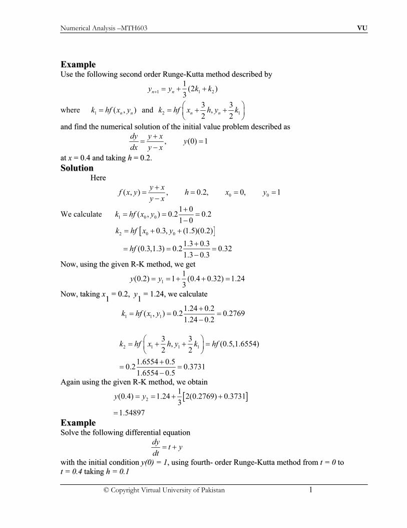
Numerical Analysis –MTH603 VU
© Copyright Virtual University of Pakistan 1
EExxaammppllee UUssee tthhee ffoolllloowwiinngg sseeccoonndd oorrddeerr RRuunnggee--KKuuttttaa mmeetthhoodd ddeessccrriibbeedd bbyy
1 1 2
1(2 )
3n ny y k k !
where 1 ( , )n nk hf x y! and 2 1
3 3,
2 2n nk hf x h y k
" #! $ %& '
aanndd ffiinndd tthhee nnuummeerriiccaall ssoolluuttiioonn ooff tthhee iinniittiiaall vvaalluuee pprroobblleemm ddeessccrriibbeedd aass
, (0) 1dy y x
ydx y x
! !
(
aatt xx == 00..44 aanndd ttaakkiinngg hh == 00..22..
SSoolluuttiioonn HHeerree
0 0( , ) , 0.2, 0, 1y x
f x y h x yy x
! ! ! !
(
We calculate 1 0 0
1 0( , ) 0.2 0.2
1 0k hf x y
! ! !
(
) *2 0 00.3, (1.5)(0.2)
1.3 0.3(0.3,1.3) 0.2 0.32
1.3 0.3
k hf x y
hf
!
! ! !
(
NNooww,, uussiinngg tthhee ggiivveenn RR--KK mmeetthhoodd,, wwee ggeett
1
1(0.2) 1 (0.4 0.32) 1.24
3y y! ! !
NNooww,, ttaakkiinngg xx11 == 00..22,, yy
11 == 11..2244,, wwee ccaallccuullaattee
1 1 1
1.24 0.2( , ) 0.2 0.2769
1.24 0.2k hf x y
! ! !
(
2 1 1 1
3 3, (0.5,1.6554)
2 2
1.6554 0.50.2 0.3731
1.6554 0.5
k hf x h y k hf" #! !$ %& '
! !
(
AAggaaiinn uussiinngg tthhee ggiivveenn RR--KK mmeetthhoodd,, wwee oobbttaaiinn
) *2
1(0.4) 1.24 2(0.2769) 0.3731
3
1.54897
y y! !
!
EExxaammppllee SSoollvvee tthhee ffoolllloowwiinngg ddiiffffeerreennttiiaall eeqquuaattiioonn
dy
t ydt
!
wwiitthh tthhee iinniittiiaall ccoonnddiittiioonn yy((00)) == 11,, uussiinngg ffoouurrtthh-- oorrddeerr RRuunnggee--KKuuttttaa mmeetthhoodd ffrroomm tt == 00 ttoo
tt == 00..44 ttaakkiinngg hh == 00..11

Numerical Analysis –MTH603 VU
© Copyright Virtual University of Pakistan 2
SSoolluuttiioonn TThhee ffoouurrtthh--oorrddeerr RRuunnggee--KKuuttttaa mmeetthhoodd iiss ddeessccrriibbeedd aass
1 1 2 3 4
1( 2 2 )
6n ny y k k k k ! (1)
Where
1
12
23
4 3
( , )
,2 2
,2 2
( , )
n n
n n
n n
n n
k hf t y
khk hf t y
khk hf t y
k hf t h y k
!
" #! $ %& '
" #! $ %& '
!
In this problem
0 0( , ) , 0.1, 0, 1.f t y t y h t y! ! ! !
AAss aa ffiirrsstt sstteepp,, wwee ccaallccuullaattee
1 0 0
2 0 0
3 0 0
4
( , ) 0.1(1) 0.1
( 0.05, 0.05)
(0.05,1.05) 0.1[0.05 1.05]
0.11
( 0.05, 0.055)
0.1(0.05 1.055)
0.1105
0.1(0.1 1.1105) 0.12105
k hf t y
k hf t y
hf
k hf t y
k
! ! !
!
! !
!
!
!
!
! !
NNooww,, wwee ccoommppuuttee ffrroomm
1 0 1 2 3 4
1( 2 2 )
6
11 (0.1 0.22 0.2210 0.12105)
6
1.11034
y y k k k k!
!
!
TThheerreeffoorree yy((00..11)) == yy11==11..11110033
IInn tthhee sseeccoonndd sstteepp,, wwee hhaavvee ttoo ffiinndd yy22
== yy((00..22))
We compute

Numerical Analysis –MTH603 VU
© Copyright Virtual University of Pakistan 3
1 1 1
12 1 1
23 1 1
4 1 1 3
( , ) 0.1(0.1 1.11034) 0.121034
,2 2
0.1[0.15 (1.11034 0.060517)] 0.13208
,2 2
0.1[0.15 (1.11034 0.06604)] 0.132638
( , )
0.1[0.2 (1.11034 0.13263
k hf t y
khk hf t y
khk hf t y
k hf t h y k
! ! !
" #! $ %& '
! !
" #! $ %& '
! !
!
! 8)] 0.1442978!
FFrroomm EEqquuaattiioonn ((11)),, wwee sseeee tthhaatt
2
11.11034 [0.121034 2(0.13208)
6
2(0.132638) 0.1442978] 1.2428
y !
!
SSiimmiillaarrllyy wwee ccaallccuullaattee,,
1 2 2
12 2 2
23 1 1
4 2 2 3
( , ) 0.1[0.2 1.2428] 0.14428
, 0.1[0.25 (1.2428 0.07214)] 0.1564942 2
, 0.1[0.3 (1.2428 0.078247)] 0.15710472 2
( , ) 0.1[0.3 (1.2428 0.1571047)]
k hf t y
khk hf t y
khk hf t y
k hf t h y k
! ! !
" #! ! !$ %& '
" #! ! !$ %& '
! ! 0.16999047!
UUssiinngg eeqquuaattiioonn ((11)),, wwee ccoommppuuttee
3 2 1 2 3 4
1(0.3) ( 2 2 ) 1.399711
6y y y k k k k! ! !
FFiinnaallllyy,, wwee ccaallccuullaattee
1 3 3
12 3 3
23 3 3
4 3 3 3
( , ) 0.1[0.3 1.3997] 0.16997
, 0.1[0.35 (1.3997 0.084985)] 0.18346852 2
, 0.1[0.35 (1.3997 0.091734)] 0.18414342 2
( , ) 0.1[0.4 (1.3997 0.184143
k hf t y
khk hf t y
khk hf t y
k hf t h y k
! ! !
" #! ! !$ %& '
" #! ! !$ %& '
! ! 4)] 0.19838434!
UUssiinngg tthheemm iinn eeqquuaattiioonn ((11)),, wwee ggeett
4 3 1 2 3 4
1(0.4) ( 2 2 )
6
1.58363
y y y k k k k! !
!
wwhhiicchh iiss tthhee rreeqquuiirreedd rreessuulltt..
EExxaammppllee
Apply Runge-Kutta Method of order four to solve the initial value problem at x=1.2
/ 1/3 ; (1) 1 ; 0.1y xy y h! ! !

Numerical Analysis –MTH603 VU
© Copyright Virtual University of Pakistan 4
Solution:
The Fourth-Order Runge-Kutta Method is described as :-
+ ,
+ ,
+ ,
1 1 2 3 4
1
12
23
4 3
12 2
6
,
,
,2 2
,2 2
,
n n
n n
n n
n n
n n
y y k k k k
where
k hf t y
khk hf t y
khk hf t y
k hf t h y k
!
!
" #! $ %& '
" #! $ %& '
!
( Here, we are taking x as t )
First Iteration:-

Numerical Analysis –MTH603 VU
© Copyright Virtual University of Pakistan 5
+ , + ,
+ , + ,
+ ,
+ , + ,
0 0
1/3
1 0 0
12
1/3
1
23
1/3
2
4 3
1/3
3
1 , 1
( , ) 0.1 1 1
0.1
,2 2
0.1 1 0.05 1 / 2
0.106721617
,2 2
0.1 1 0.05 1 / 2
0.10683536
,
0.1 1 0.1 1
0.11378
n n
n n
n n
t y
k hf t y
khk hf t y
k
khk hf t y
k
k hf t h y k
k
! !
- .! ! /0 1!
" #! $ %& '
- .! / 0 1!
" #! $ %& '
- .! / 0 1!
!
- .! / 0 1!
+ ,1 1 2 3 4
1
1
5527
2 2
1 0.10681658
1.10681658
n ny y k k k k
y
y
!
!
!
Second Iteration:-

Numerical Analysis –MTH603 VU
© Copyright Virtual University of Pakistan 6
+ , + ,
+ , + ,
1 1
1/3
1 1 1
12
1/3
23
1/3
2
1.1 , 1.10681658
( , ) 0.1 1.1 1.10681658
0.113784884
,2 2
0.1 1.1 0.05 1 1.10681658 / 2
0.120961169
,2 2
0.1 1.1 0.05 1.10681658 / 2
0.1
n n
n n
t y
k hf t y
khk hf t y
khk hf t y
k
! !
- .! ! /0 1!
" #! $ %& '
- .! / 0 1!
" #! $ %& '
- .! / 0 1!
+ ,
+ , + ,
+ ,
4 3
1/3
3
1 1 2 3 4
2
2
21085364
,
0.1 1.1 0.1 1.10681658
0.128499807
2 2
1.10681658 0.12106296
1.22787954
n n
n n
k hf t h y k
k
y y k k k k
y
y
!
- .! / 0 1!
!
!
!
So, at x = 1.2 , we get:
y(1.2) = y2 = 1.22787954
RRUUNNGGEE –– KKUUTTTTAA MMEETTHHOODD FFOORR SSOOLLVVIINNGG AA SSYYSSTTEEMM OOFF
EEQQUUAATTIIOONNSS TThhee ffoouurrtthh--oorrddeerr RRuunnggee--KKuuttttaa mmeetthhoodd ccaann bbee eexxtteennddeedd ttoo nnuummeerriiccaallllyy ssoollvvee tthhee hhiigghheerr--
oorrddeerr oorrddiinnaarryy ddiiffffeerreennttiiaall eeqquuaattiioonnss-- lliinneeaarr oorr nnoonn--lliinneeaarr
FFoorr iilllluussttrraattiioonn,, lleett uuss ccoonnssiiddeerr aa sseeccoonndd oorrddeerr oorrddiinnaarryy ddiiffffeerreennttiiaall eeqquuaattiioonn ooff tthhee ffoorrmm
2
2, ,
d y dyf t y
dt dt
" #! $ %& '

Numerical Analysis –MTH603 VU
© Copyright Virtual University of Pakistan 7
UUssiinngg tthhee ssuubbssttiittuuttiioonn dy
pdt
! tthhiiss eeqquuaattiioonn ccaann bbee rreedduucceedd ttoo ttwwoo ffiirrsstt--oorrddeerr
ssiimmuullttaanneeoouuss ddiiffffeerreennttiiaall eeqquuaattiioonnss,, aass ggiivveenn bbyy
1 2( , , ), ( , , )dy dp
p f t y p f t y pdt dt
! ! !
NNooww,, wwee ccaann ddiirreeccttllyy wwrriittee ddoowwnn tthhee RRuunnggee--KKuuttttaa ffoouurrtthh--oorrddeerr
ffoorrmmuullaaee ffoorr ssoollvviinngg tthhee ssyysstteemm..
LLeett tthhee iinniittiiaall ccoonnddiittiioonnss ooff tthhee aabboovvee ssyysstteemm bbee ggiivveenn bbyy
( ) , ( ) ( )n n n n ny x y y x p x p2! ! !
Then we define
+ ,1 1 1 2
1 1 1 12 1 2 2
2 2 2 23 1 3 2
4 1 3 3 4 2 3
, , , ( , , )
, , , , ,2 2 2 2 2 2
, , , , ,2 2 2 2 2 2
( , , ), ( , ,
n n n n n n
n n n n n n
n n n n n n
n n n n n
k hf t y p l hf t y p
k l k lh hk hf t y p l hf t y p
k l k lh hk hf t y p l hf t y p
k hf t h y k p l l hf t h y k
! !
" # " #! ! $ % $ %& ' & '
" # " #! ! $ % $ %& ' & '
! ! 3)np l
344445444
46
NNooww,, uussiinngg tthhee iinniittiiaall ccoonnddiittiioonnss yynn,, pp
nn aanndd 44
tthh --oorrddeerr RR--KK ffoorrmmuullaa,, wwee ccoommppuuttee
1 1 2 3 4
1 1 2 3 4
1( 2 2 )
6
1( 2 2 )
6
n n
n n
y y k k k k
p p l l l l
3! 4454! 46
TThhiiss mmeetthhoodd ccaann bbee eexxtteennddeedd oonn ssiimmiillaarr lliinneess ttoo ssoollvvee ssyysstteemm ooff nn ffiirrsstt oorrddeerr ddiiffffeerreennttiiaall
eeqquuaattiioonnss..
EExxaammppllee SSoollvvee tthhee ffoolllloowwiinngg eeqquuaattiioonn
2(0.1)(1 ) 0y y y y22 2( ( !
UUssiinngg 44tthh
oorrddeerr RRuunnggee--KKuuttttaa mmeetthhoodd ffoorr xx == 00..22,, wwiitthh tthhee iinniittiiaall vvaalluueess yy((00)) == 11,, yy’’((00))==00
Solution:
Let 1( , , )dy
p f x y pdx
! !
Then 2 2(0.1)(1 ) ( , , )dp
y p y f x y pdx
! ( ( !
TThhuuss,, tthhee ggiivveenn eeqquuaattiioonn rreedduucceedd ttoo ttwwoo ffiirrsstt--oorrddeerr eeqquuaattiioonnss..
IInn tthhee pprreesseenntt pprroobblleemm,, wwee aarree ggiivveenn
xx00 == 00,, yy
00 == 11,, pp
00 ==yy
oo’’ ==00
TTaakkiinngg hh == 00..22,, wwee ccoommppuuttee

Numerical Analysis –MTH603 VU
© Copyright Virtual University of Pakistan 8
1 1 0 0 0
1 2 0 0 0
1 12 1 0 0 0
2
1 12 2 0 0 0
2
( , , ) 0.2(0.0) 0.0
( , , ) 0.2(0.0 1) 0.2
, ,2 2 2
(0.1,1.0, 0.1) 0.02
, ,2 2 2
(0.1,1.0, 0.1) 0.2( 0.1) 0.02
k hf x y p
l hf x y p
k lhk hf x y p
hf
k lhl hf x y p
hf
! !
" # $ $ $% &
' (
! !
" # $ $ $% &
' (
! ! !
2 23 1 0 0 0
1
2 23 2 0 0 0 2
4 1 0 0 3 0 3
1
, ,2 2 2
(0.1,0.99, 0.1) 0.2( 0.1) 0.02
, , (0.1,0.99, 0.1)2 2 2
0.2[(0.1)(0.0199)( 0.1) 0.99] 0.1980
( , , )
(0.2,0.98, 0.1980)
k lhk hf x y p
hf
k lhl hf x y p hf
k hf x h y k p l
hf
" # $ $ $% &
' (
! ! !
" # $ $ $ !% &
' (
! ! !
$ $ $
!
4 2 0 0 3 0 3 2
0.0396
( , , ) (0.2,0.98, 0.1980)
0.2[(0.1)(1 0.9604)( 0.1980) 0.98] 0.19616
l hf x h y k p l hf
!
$ $ $ !
! ! ! !
NNooww,, yy ((00..22)) == yy11 iiss ggiivveenn bbyy
1 0 1 2 3 4
1(0.2) [ 2 2 ]
6y y y k k k k $ $ $ $
1
1 [0.0 2( 0.02) 2( 0.02) ( 0.0396)]6
$ $ ! $ ! $ !
1 0.019935 0.9801 !
1 0 1 2 3 4
1(0.2) [ 2 2 ]
6y p p l l l l) $ $ $ $
1
0 [ 0.2 2( 0.2) 2( 0.1980) ( 0.19616)]6
$ ! $ ! $ ! $ !
0.19869( 0.1987) ! !
TThheerreeffoorree,, tthhee rreeqquuiirreedd ssoolluuttiioonn iiss
(0.2) 0.9801, (0.2) 0.1987y y) !

Numerical Analysis –MTH603 VU
© Copyright Virtual University of Pakistan 1
PPRREEDDIICCTTOORR –– CCOORRRREECCTTOORR MMEETTHHOODD TThhee mmeetthhooddss pprreesseenntteedd ssoo ffaarr aarree ccaalllleedd ssiinnggllee--sstteepp mmeetthhooddss,, wwhheerree wwee hhaavvee sseeeenn tthhaatt tthhee
ccoommppuuttaattiioonn ooff yy aatt ttnn++11
tthhaatt iiss yynn++11
rreeqquuiirreess tthhee kknnoowwlleeddggee ooff yynn oonnllyy..
IInn pprreeddiiccttoorr--ccoorrrreeccttoorr mmeetthhooddss wwhhiicchh wwee wwiillll ddiissccuussss nnooww,, iiss aallssoo kknnoowwnn aass mmuullttii--sstteepp
mmeetthhooddss..
TToo ccoommppuuttee tthhee vvaalluuee ooff yy aatt ttnn++11
,, wwee mmuusstt kknnooww tthhee ssoolluuttiioonn yy aatt ttnn
,, ttnn--11
,, ttnn--22
,, eettcc..
TThhuuss,, aa pprreeddiiccttoorr ffoorrmmuullaa iiss uusseedd ttoo pprreeddiicctt tthhee vvaalluuee ooff yy aatt ttnn++11
aanndd tthheenn aa ccoorrrreeccttoorr
ffoorrmmuullaa iiss uusseedd ttoo iimmpprroovvee tthhee vvaalluuee ooff yynn++11
..
LLeett uuss ccoonnssiiddeerr aann IIVVPP
( , ), ( )n n
dyf t y y t y
dt
UUssiinngg ssiimmppllee EEuulleerr’’ss aanndd mmooddiiffiieedd EEuulleerr’’ss mmeetthhoodd,, wwee ccaann wwrriittee ddoowwnn aa ssiimmppllee
pprreeddiiccttoorr--ccoorrrreeccttoorr ppaaiirr
((PP –– CC)) aass
(0)
1
(1) (0)
1 1 1
: ( , )
: ( , ) ( , )2
n n n n
n n n n n n
P y y hf t y
hC y y f t y f t y
!
! ! !
" !#$
% & ! ! #' ()
HHeerree,, yynn++11
((11)) iiss tthhee ffiirrsstt ccoorrrreecctteedd vvaalluuee ooff yy
nn++11.. TThhee ccoorrrreeccttoorr ffoorrmmuullaa mmaayy bbee
uusseedd iitteerraattiivveellyy aass ddeeffiinneedd bbeellooww::
( ) ( 1)
1 1 1( , ) ( , ) , 1, 2,2
r r
n n n n n n
hy y f t y f t y r*
! ! !% & ! ! ' (
TThhee iitteerraattiioonn iiss tteerrmmiinnaatteedd wwhheenn ttwwoo ssuucccceessssiivvee iitteerraatteess aaggrreeee ttoo tthhee ddeessiirreedd aaccccuurraaccyy
IInn tthhiiss ppaaiirr,, ttoo eexxttrraappoollaattee tthhee vvaalluuee ooff yynn++11
,, wwee hhaavvee aapppprrooxxiimmaatteedd tthhee ssoolluuttiioonn ccuurrvvee iinn
tthhee iinntteerrvvaall ((ttnn,, tt
nn++11)) bbyy aa ssttrraaiigghhtt lliinnee ppaassssiinngg tthhrroouugghh ((tt
nn,, yy
nn)) aanndd ((tt
nn++11,, yy
nn++11))..
TThhee aaccccuurraaccyy ooff tthhee pprreeddiiccttoorr ffoorrmmuullaa ccaann bbee iimmpprroovveedd bbyy ccoonnssiiddeerriinngg aa qquuaaddrraattiicc ccuurrvvee
tthhrroouugghh tthhee eeqquuaallllyy ssppaacceedd ppooiinnttss ((ttnn--11
,, yynn--11
)),, ((ttnn,, yy
nn)),, ((tt
nn++11,, yy
nn++11))
SSuuppppoossee wwee ffiitt aa qquuaaddrraattiicc ccuurrvvee ooff tthhee ffoorrmm
1 1( ) ( )( )n n ny a b t t c t t t t* * ! * ! * *
wwhheerree aa,, bb,, cc aarree ccoonnssttaannttss ttoo bbee ddeetteerrmmiinneedd AAss tthhee ccuurrvvee ppaasssseess tthhrroouugghh
((ttnn--11
,, yynn--11
)) aanndd ((ttnn,, yy
nn)) aanndd ssaattiissffiieess
( , )
( , )
n n
n n
t y
dyf t y
dt
+ , - .
/ 0
We obtain 1 1,n n ny a y a bh y bh* * ! !
Therefore
1n ny yb
h
**
and

Numerical Analysis –MTH603 VU
© Copyright Virtual University of Pakistan 2
1 ( , )
( , )
( , ) { [( ) ( )]}n n
n n
n n n n t y
t y
dyf t y b c t t t t
dt*
+ , ! * ! *- .
/ 0
Which give
1( , ) ( )n n n nf t y b c t t b ch* ! * !
or 1
2
( , ) ( )n n n nf t y y yc
h h
** *
SSuubbssttiittuuttiinngg tthheessee vvaalluueess ooff aa,, bb aanndd cc iinnttoo tthhee qquuaaddrraattiicc eeqquuaattiioonn,, wwee ggeett
1 1 1 12( ) 2[ ( , ) ( )]n n n n n n n ny y y y hf t y y y! * * * ! * ! * *
That is
1 1 2 ( , )n n n ny y hf t y! * !
TThhuuss,, iinnsstteeaadd ooff ccoonnssiiddeerriinngg tthhee PP--CC ppaaiirr,, wwee mmaayy ccoonnssiiddeerr tthhee PP--CC ppaaiirr ggiivveenn bbyy
1 1
1 1 1
: 2 ( , )
: [ ( , ) ( , )]2
n n n n
n n n n n n
P y y hf t y
hC y y f t y f t y
! *
! ! !
! "#$
! ! #)
TThhee eesssseennttiiaall ddiiffffeerreennccee bbeettwweeeenn tthheemm iiss,, tthhee oonnee ggiivveenn aabboovvee iiss mmoorree aaccccuurraattee
HHoowweevveerr,, tthhiiss oonnee ccaann nnoott bbee uusseedd ttoo pprreeddiicctt yynn++11
ffoorr aa ggiivveenn IIVVPP,, bbeeccaauussee iittss uussee
rreeqquuiirree tthhee kknnoowwlleeddggee ooff ppaasstt ttwwoo ppooiinnttss.. IInn ssuucchh aa ssiittuuaattiioonn,, aa RR--KK mmeetthhoodd iiss ggeenneerraallllyy
uusseedd ttoo ssttaarrtt tthhee pprreeddiiccttoorr mmeetthhoodd..
MMiillnnee’’ss MMeetthhoodd IItt iiss aallssoo aa mmuullttii--sstteepp mmeetthhoodd wwhheerree wwee aassssuummee tthhaatt tthhee ssoolluuttiioonn ttoo tthhee ggiivveenn IIVVPP iiss
kknnoowwnn aatt tthhee ppaasstt ffoouurr eeqquuaallllyy ssppaacceedd ppooiinntt tt00,, tt
11,, tt
22 aanndd tt
33..
TToo ddeerriivvee MMiillnnee’’ss pprreeddiiccttoorr--ccoorrrreeccttoorr ppaaiirr,, lleett uuss ccoonnssiiddeerr aa ttyyppiiccaall IIVVPP
0 0( , ), ( )dy
f t y y t ydt
OOnn iinntteeggrraattiioonn bbeettwweeeenn tthhee lliimmiittss tt00 aanndd tt
44,, wwee ggeett
4 4
0 0
( , )t t
t t
dydt f t y dt
dt 1 1
4
04 0 ( , )
t
ty y f t y dt* 1
BBuutt wwee kknnooww ffrroomm NNeewwttoonn’’ss ffoorrwwaarrdd ddiiffffeerreennccee ffoorrmmuullaa
2 3
0 0 0 0
( 1) ( 1)( 2)( , )
2 6
s s s s sf t y f s f f f
* * * ! 2 ! 2 ! 2 !!
where 00,
t ts t t sh
h
* !
4
0
2 3
4 0 0 0 0 0
4
0
( 1) ( 1)( 2)
2 6
( 1( 2)( 3)
24
t
t
s s s s sy y f s f f f
s s s sf dt
* * *% ! ! 2 ! 2 ! 23'
* * * &! 2 ! 4(
1
!
NNooww,, bbyy cchhaannggiinngg tthhee vvaarriiaabbllee ooff iinntteeggrraattiioonn ((ffrroomm tt ttoo ss)),, tthhee lliimmiittss ooff iinntteeggrraattiioonn aallssoo
cchhaannggeess ((ffrroomm 00 ttoo 44)),, aanndd tthhuuss tthhee aabboovvee eexxpprreessssiioonn bbeeccoommeess

Numerical Analysis –MTH603 VU
© Copyright Virtual University of Pakistan 3
42 3
4 0 0 0 0 00
4
0
( 1) ( 1)( 2)4
2 6
( 1( 2)( 3)
24
s s s s sy y h f s f f f
s s s sf ds
* * *% ! ! 2 ! 2 ! 23'
* * * &! 2 ! 4(
1
!
wwhhiicchh ssiimmpplliiffiieess ttoo
2 3 4
4 0 0 0 0 0 0
20 8 284 8
3 3 90y y h f f f f f
% & ! ! 2 ! 2 ! 2 ! 23 4' (
SSuubbssttiittuuttiinngg tthhee ddiiffffeerreenncceess
2
0 1 0 0 2 1 0, 2 ,f f f f f f f2 * 2 * !
IItt ccaann bbee ffuurrtthheerr ssiimmpplliiffiieedd ttoo
4
4 0 1 2 3 0
4 28(2 2 )
3 90
hy y f f f h f ! * ! ! 2
AAlltteerrnnaattiivveellyy,, iitt ccaann aallssoo bbee wwrriitttteenn aass
4
4 0 1 2 3 0
4 28(2 2 )
3 90
hy y y y y h y5 5 5 5 ! * ! ! 2
TThhiiss iiss kknnoowwnn aass MMiillnnee’’ss pprreeddiiccttoorr ffoorrmmuullaa..
SSiimmiillaarrllyy,, iinntteeggrraattiinngg tthhee oorriiggiinnaall oovveerr tthhee iinntteerrvvaall tt00 ttoo tt
22 oorr ss == 00 ttoo 22 aanndd rreeppeeaattiinngg tthhee
aabboovvee sstteeppss,, wwee ggeett
4
2 0 0 1 2 0
1( 4 )
3 90
hy y y y y h y ! " " " # $
wwhhiicchh iiss kknnoowwnn aass MMiillnnee’’ss ccoorrrreeccttoorr ffoorrmmuullaa..
IInn ggeenneerraall,, MMiillnnee’’ss pprreeddiiccttoorr--ccoorrrreeccttoorr ppaaiirr ccaann bbee wwrriitttteenn aass
1 3 2 1
1 1 1 1
4: (2 2 )
3
: ( 4 )3
n n n n n
n n n n n
hP y y y y y
hC y y y y y
" # # #
" # # "
% ! " # " &&'& ! " " "&(
FFrroomm tthheessee eeqquuaattiioonnss,, wwee oobbsseerrvvee tthhaatt tthhee mmaaggnniittuuddee ooff tthhee ttrruunnccaattiioonn eerrrroorr iinn
ccoorrrreeccttoorr ffoorrmmuullaa iiss 4 /
01/ 90h y$ wwhhiillee tthhee ttrruunnccaattiioonn eerrrroorr iinn pprreeddiiccttoorr ffoorrmmuullaa iiss 4 /
028 / 90h y$
TThhuuss:: TTEE iinn,, cc--ffoorrmmuullaa iiss lleessss tthhaann tthhee TTEE iinn pp--ffoorrmmuullaa..
IInn oorrddeerr ttoo aappppllyy tthhiiss PP –– CC mmeetthhoodd ttoo ssoollvvee nnuummeerriiccaallllyy aannyy iinniittiiaall vvaalluuee pprroobblleemm,, wwee
ffiirrsstt pprreeddiicctt tthhee vvaalluuee ooff yynn++11
bbyy mmeeaannss ooff pprreeddiiccttoorr ffoorrmmuullaa,, wwhheerree ddeerriivvaattiivveess aarree
ccoommppuutteedd uussiinngg tthhee ggiivveenn ddiiffffeerreennttiiaall eeqquuaattiioonn iittsseellff..
UUssiinngg tthhee pprreeddiicctteedd vvaalluuee yynn++11
,, wwee ccaallccuullaattee tthhee ddeerriivvaattiivve yy’’nn++11
frroomm tthhee ggiivveenn
ddiiffffeerreennttiiaall eeqquuaattiioonn aanndd tthheenn wwee uussee tthhee ccoorrrreeccttoorr ffoorrmmuullaa ooff tthhee ppaaiirr ttoo hhaavvee tthhee
ccoorrrreecctteedd vvaalluuee ooff yynn++11
TThhiiss iinn ttuurrnn mmaayy bbee uusseedd ttoo oobbttaaiinn iimmpprroovveedd vvaalluuee ooff yynn++11
bbyy
uussiinngg ccoorrrreeccttoorr aaggaaiinn.. TThhiiss iinn ttuurrnn mmaayy bbee uusseedd ttoo oobbttaaiinn iimmpprroovveedd vvaalluuee ooff yynn++11
bbyy
uussiinngg tthhee ccoorrrreeccttoorr aaggaaiinn.. TThhiiss ccyyccllee iiss rreeppeeaatteedd uunnttiill wwee aacchhiieevvee tthhee rreeqquuiirreedd aaccccuurraaccyy..
EExxaammppllee

Numerical Analysis –MTH603 VU
© Copyright Virtual University of Pakistan 4
FFiinndd yy ((22..00)) iiff yy (( tt )) iiss tthhee ssoolluuttiioonn ooff 1
( )2
dyt y
dt! "
yy ((00)) == 22,, yy ((00..55)) == 22..663366,,
yy ((11..00)) == 33..559955 aanndd yy((11..55)) == 44..996688 UUssee MMiillnnee’’ss PP--CC mmeetthhoodd..
SSoolluuttiioonn
TTaakkiinngg tt00 == 00..00,, tt
11 == 00..55,, tt
22 == 11..00,, tt
33 == 11..55 yy
00,, yy
11,, yy
22 aanndd yy
33,, aarree ggiivveenn,, wwee hhaavvee ttoo
ccoommppuuttee yy44,, tthhee ssoolluuttiioonn ooff tthhee ggiivveenn ddiiffffeerreennttiiaall eeqquuaattiioonn ccoorrrreessppoonnddiinngg ttoo tt ==22..00
TThhee MMiillnnee’’ss PP –– CC ppaaiirr iiss ggiivveenn aass
1 3 2 1
1 1 1 1
4: (2 2 )
3
: ( 4 )3
n n n n n
n n n n n
hP y y y y y
hC y y y y y
" # # #
" # # "
! " # "
! " " "
FFrroomm tthhee ggiivveenn ddiiffffeerreennttiiaall eeqquuaattiioonn,, ( ) / 2y t y ! "
WWee hhaavvee
1 11
2 22
3 33
0.5 2.6361.5680
2 2
1.0 3.5952.2975
2 2
1.5 4.9683.2340
2 2
t yy
t yy
t yy
" " ! ! !
" " ! ! !
" " ! ! !
NNooww,, uussiinngg pprreeddiiccttoorr ffoorrmmuullaa,, wwee ccoommppuuttee
) *
4 0 1 2 3
4(2 2 )
3
4(0.5)2 2(1.5680) 2.2975 2(3.2340)
3
6.8710
hy y y y y ! " # "
! " # "
!
UUssiinngg tthhiiss pprreeddiicctteedd vvaalluuee,, wwee sshhaallll ccoommppuuttee tthhee iimmpprroovveedd vvaalluuee ooff yy44 ffrroomm ccoorrrreeccttoorr
ffoorrmmuullaa
4 2 2 3 4( 4 )3
hy y y y y ! " " "
UUssiinngg tthhee aavvaaiillaabbllee pprreeddiicctteedd vvaalluuee yy44 aanndd tthhee iinniittiiaall vvaalluueess,, wwee ccoommppuuttee
4 44
3 33
2
2 6.687104.4355
2 2
1.5 4.9683.2340
2 2
2.2975
t yy
t yy
and y
" " ! ! !
" " ! ! !
!
TThhuuss,, tthhee ffiirrsstt ccoorrrreecctteedd vvaalluuee ooff yy44 iiss ggiivveenn bbyy

Numerical Analysis –MTH603 VU
© Copyright Virtual University of Pakistan 5
(1)
4
0.53.595 [2.2975 4(3.234) 4.4355]
3
6.8731667
y ! " " "
!
SSuuppppoossee,, wwee aappppllyy tthhee ccoorrrreeccttoorr ffoorrmmuullaa aaggaaiinn,, tthheenn wwee hhaavvee
(2) (1)
4 2 2 3 4( 4 ( )3
0.5 2 6.87316673.595 2.2975 4(3.234)
3 2
6.8733467
hy y y y y + ,! " " "- .
"+ ,! " " "/ 0- .!
FFiinnaallllyy,, yy ((22..00)) == yy44 == 66..88773344..
EExxaammppllee
TTaabbuullaattee tthhee ssoolluuttiioonn ooff , (0) 1dy
t y ydt
! " ! iinn tthhee iinntteerrvvaall [[00,, 00..44]] wwiitthh hh == 00..11,,
uussiinngg MMiillnnee’’ss PP--CC mmeetthhoodd..
SSoolluuttiioonn MMiillnnee’’ss PP--CC mmeetthhoodd ddeemmaanndd tthhee ssoolluuttiioonn aatt ffiirrsstt ffoouurr ppooiinnttss tt
00,, tt
11,, tt
22 aanndd tt
33.. AAss iitt iiss nnoott aa
sseellff –– ssttaarrttiinngg mmeetthhoodd,, wwee sshhaallll uussee RR--KK mmeetthhoodd ooff ffoouurrtthh oorrddeerr ttoo ggeett tthhee rreeqquuiirreedd
ssoolluuttiioonn aanndd tthheenn sswwiittcchh oovveerr ttoo MMiillnnee’’ss PP –– CC mmeetthhoodd..
TThhuuss,, ttaakkiinngg tt00 == 00,, tt
11 == 00..11,, tt
22 == 00..22,, tt
33 == 00..33 wwee ggeett tthhee ccoorrrreessppoonnddiinngg yy vvaalluueess uussiinngg
RR––KK mmeetthhoodd ooff 44tthh
oorrddeerr;; tthhaatt iiss yy00 == 11,, yy
11 == 11..11110033,, yy
22 == 11..22442288 aanndd yy
33 == 11..33999977
((RReeffeerreennccee LLeeccttuurree 3388))
Now we compute
1 1 1
2 2 2
3 3 3
0.1 1.1103 1.2103
0.2 1.2428 1.4428
0.3 1.3997 1.6997
y t y
y t y
y t y
! " ! " !
! " ! " !
! " ! " !
UUssiinngg MMiillnnee’’ss pprreeddiiccttoorr ffoorrmmuullaa
# $
4 0 1 2 3
4: (2 2 )
3
4(0.5)1 2(1.21103) 1.4428 2(1.69971)
3
1.58363
hP y y y y y ! " % "
! " % "
!
BBeeffoorree uussiinngg ccoorrrreeccttoorr ffoorrmmuullaa,, wwee ccoommppuuttee
4 4 4 ( )
0.4 1.5836 1.9836
y t y predicted value ! "
! " !
FFiinnaallllyy,, uussiinngg MMiillnnee’’ss ccoorrrreeccttoorr ffoorrmmuullaa,, wwee ccoommppuuttee

Numerical Analysis –MTH603 VU
© Copyright Virtual University of Pakistan 6
4 2 4 3 2: ( 4 )3
0.11.2428 (1.9836 6.7988 1.4428)
3
1.5836
hC y y y y y ! " " "
! " " "
!
TThhee rreeqquuiirreedd ssoolluuttiioonn iiss::
t 0 0.1 0.2 0.3 0.4
y 1 1.1103 1.2428 1.3997 1.5836
Example Using Milne’s Predictor-Corrector Formula find f(0.4) from Ordinary Differential
Equation
/ ; (0) 1 ; 0.1y x y y h! % ! !
with the help of following table.
Solution:
& '
& '
0 1 2 3 4
1 1 1
2 2 2
3 3 3
4 0 1 2 3
4
4
,
0 , 0.1 , 0.2 , 0.3 , 0.4
' 0.1 0.9097 0.8097
' 0.2 0.8375 0.6375
' 0.3 0.7816 0.4816
4y 2 ' ' 2 '
3
4*0.1y 1 -1.9451
3
y 0.740653333
Here
x x x x x
y x y
y x y
y x y
Now, using Predictor Formula
hy y y y
! ! ! ! !
! % ! % ! %
! % ! % ! %
! % ! % ! %
! " % "
! "
!
X 0 0.1 0.2 0.3
Y 1 0.9097 0.8375 0.7816

Numerical Analysis –MTH603 VU
© Copyright Virtual University of Pakistan 7
Using the predicted value, we shall now compute the corrected value as;
& '
& '
& '& '
4 2 2 3 4
4 4 4
4 2 2 3 4
4
4
4
' 4 ' '3
,
' 0.4 0.740653333= 0.340653333
,int ;
' 4 ' '3
0.10.8375+ 0.6375+ 4* 0.4816 0.340653333
3
0.8375 0.096818444
0.74068155
hy y y y y
Now
y x y
Putting the values o the Corrector Formula
hy y y y y
y
y
y
! " " "
! % ! %
! " " "
! % %
!
!
-
-
-
6 Ans.

Numerical Analysis –MTH603 VU
© Copyright Virtual University of Pakistan 8

Numerical Analysis –MTH603 VU
© Copyright Virtual University of Pakistan 1
AAddaamm--MMoouullttoonn MMeetthhoodd
IItt iiss aannootthheerr pprreeddiiccttoorr--ccoorrrreeccttoorr mmeetthhoodd,, wwhheerree wwee uussee tthhee ffaacctt tthhaatt tthhee ssoolluuttiioonn ttoo tthhee
ggiivveenn iinniittiiaall vvaalluuee pprroobblleemm iiss kknnoowwnn aatt ppaasstt ffoouurr eeqquuaallllyy ssppaacceedd ppooiinnttss
ttnn
,, ttnn--11
,, ttnn--22
,, ttnn--33
..
TThhee ttaasskk iiss ttoo ccoommppuuttee tthhee vvaalluuee ooff yy aatt ttnn++11
..
LLeett uuss ccoonnssiiddeerr tthhee ddiiffffeerreennttiiaall eeqquuaattiioonn
( , )dy
f t ydt
IInntteeggrraattiinngg bbeettwweeeenn tthhee lliimmiittss ttnn ttoo tt
nn++11,, wwee hhaavvee
1 1
( , )n n
n n
t t
t t
dydt f t y dt
dt
! !
" "
TThhaatt iiss
1
1 ( , )n
n
t
n nt
y y f t y dt!
! # "
TToo ccaarrrryy oouutt iinntteeggrraattiioonn,, wwee pprroocceeeedd aass ffoolllloowwss.. WWee eemmppllooyy NNeewwttoonn’’ss bbaacckkwwaarrdd
iinntteerrppoollaattiioonn ffoorrmmuullaa,, ssoo tthhaatt
2 3( 1) ( 1)( 2)
( , )2 6
n n n n
s s s s sf t y f s f f f
! ! ! ! $ ! $ ! $ !
Where
nt ts
h#
AAfftteerr ssuubbssttiittuuttiioonn,, wwee oobbttaaiinn
%1 2
1
3 4
( 1)
2
( 1)( 2) ( 1)( 2)( 3)
6 24
n
n
t
n n n n nt
n n
s sy y f s f f
s s s s s s sf f dt
!
!
! ! ! $ ! $
! ! ! ! ! &! $ ! $ ! '(
"
NNooww bbyy cchhaannggiinngg tthhee vvaarriiaabbllee ooff iinntteeggrraattiioonn ((ffrroomm tt ttoo ss)),, tthhee lliimmiittss ooff iinntteeggrraattiioonn aallssoo
cchhaannggeess ((ffrroomm 00 ttoo 11)),, aanndd tthhuuss tthhee aabboovvee eexxpprreessssiioonn bbeeccoommeess
%1
2
10
3 4
( 1)
2
( 1)( 2) ( 1)( 2)( 3)
6 24
n n n n n
n n
s sy y h f s f f
s s s s s s sf f ds
!
! ! ! $ ! $
! ! ! ! ! &! $ ! $ ! '(
"
AAccttuuaall iinntteeggrraattiioonn rreedduucceess tthhee aabboovvee eexxpprreessssiioonn ttoo
2 3 4
1
1 5 3 251
2 12 8 720n n n n n n ny y h f f f f f!
) * ! ! $ ! $ ! $ ! $+ ,- .
NNooww ssuubbssttiittuuttiinngg tthhee ddiiffffeerreenncceess ssuucchh aass
1n n nf f f #$ #
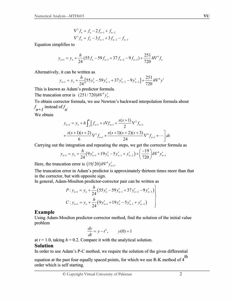
Numerical Analysis –MTH603 VU
© Copyright Virtual University of Pakistan 2
2
1 22n n n nf f f f# #$ # !
3
1 2 33 3n n n n nf f f f f# # #$ # ! #
EEqquuaattiioonn ssiimmpplliiffiieess ttoo
4
1 1 2 3
251(55 59 37 9 )
24 720n n n n n n n
hy y f f f f h f! # # # ! # ! # ! $
AAlltteerrnnaattiivveellyy,, iitt ccaann bbee wwrriitttteenn aass
% / 4
1 1 2 3
25155 59 37 9
24 720n n n n n n
hy y y y y y h y! # # #0 0 0 0 0 ! # ! # ! $
TThhiiss iiss kknnoowwnn aass AAddaamm’’ss pprreeddiiccttoorr ffoorrmmuullaa..
TThhee ttrruunnccaattiioonn eerrrroorr iiss 4(251/ 720) .nh y0$
TToo oobbttaaiinn ccoorrrreeccttoorr ffoorrmmuullaa,, wwee uussee NNeewwttoonn’’ss bbaacckkwwaarrdd iinntteerrppoollaattiioonn ffoorrmmuullaa aabboouutt
ffnn++11
iinnsstteeaadd ooff ffnn..
WWee oobbttaaiinn
%0
2
1 1 1 11
3 4
1 1
( 1)
2
( 1)( 2) ( 1)( 2)( 3)
6 24
n n n n n
n n
s sy y h f s f f
s s s s s s sf f ds
! ! ! !#
! !
! ! ! $ ! $
! ! ! ! ! &! $ ! $ ! '(
"
CCaarrrryyiinngg oouutt tthhee iinntteeggrraattiioonn aanndd rreeppeeaattiinngg tthhee sstteeppss,, wwee ggeett tthhee ccoorrrreeccttoorr ffoorrmmuullaa aass
1 2 4
1 1 1 2 1
199 19 5
24 720n n n n n n n
hy y y y y y h y! ! # # !
#) *0 0 0 0 0 ! ! # ! ! $+ ,- .
HHeerree,, tthhee ttrruunnccaattiioonn eerrrroorr iiss 1 2 4
119 20 .nh y !0$
TThhee ttrruunnccaattiioonn eerrrroorr iinn AAddaamm’’ss pprreeddiiccttoorr iiss aapppprrooxxiimmaatteellyy tthhiirrtteeeenn ttiimmeess mmoorree tthhaann tthhaatt
iinn tthhee ccoorrrreeccttoorr,, bbuutt wwiitthh ooppppoossiittee ssiiggnn..
IInn ggeenneerraall,, AAddaamm--MMoouullttoonn pprreeddiiccttoorr--ccoorrrreeccttoorr ppaaiirr ccaann bbee wwrriitttteenn aass
1 2
1 2
1 1 2 3
1 1 1 2
: 55 59 37 924
: 9 19 524
n n n n n n
n n n n n n
hP y y y y y y
hC y y y y y y
! # # #
! ! # #
30 0 0 0 ! # ! # 44540 0 0 0 ! ! # !46
EExxaammppllee UUssiinngg AAddaamm--MMoouullttoonn pprreeddiiccttoorr--ccoorrrreeccttoorr mmeetthhoodd,, ffiinndd tthhee ssoolluuttiioonn ooff tthhee iinniittiiaall vvaalluuee
pprroobblleemm
2 , (0) 1
dyy t y
dt #
aatt tt == 11..00,, ttaakkiinngg hh == 00..22.. CCoommppaarree iitt wwiitthh tthhee aannaallyyttiiccaall ssoolluuttiioonn..
SSoolluuttiioonn IInn oorrddeerr ttoo uussee AAddaamm’’ss PP--CC mmeetthhoodd,, wwee rreeqquuiirree tthhee ssoolluuttiioonn ooff tthhee ggiivveenn ddiiffffeerreennttiiaall
eeqquuaattiioonn aatt tthhee ppaasstt ffoouurr eeqquuaallllyy ssppaacceedd ppooiinnttss,, ffoorr wwhhiicchh wwee uussee RR--KK mmeetthhoodd ooff 44tthh
oorrddeerr wwhhiicchh iiss sseellff ssttaarrttiinngg..

Numerical Analysis –MTH603 VU
© Copyright Virtual University of Pakistan 3
TThhuuss ttaakkiinngg tt00 ==00,, yy
00 == 11,, hh == 00..22,, wwee ccoommppuuttee
kk11 == 00..22,, kk
22 == 00..221188,,
kk33 == 00..22119988,, kk
44 == 00..2233559966,,
aanndd ggeett
1 0 1 2 3 4
1( 2 2 ) 1.21859
6y y k k k k ! ! ! !
TTaakkiinngg tt11 == 00..22,,
yy11 == 11..2211885599,, hh == 00..22,,
wwee ccoommppuuttee kk11 == 00..2233557711,,
kk22 == 00..22449922,,
kk33 == 00..2255006644,, kk
44 == 00..2266118844,, aanndd ggeett
2 1 1 2 3 4
1( 2 2 ) 1.46813
6y y k k k k ! ! ! !
NNooww,, wwee ttaakkee tt22 == 00..44,,
yy22 == 11..4466881133,, hh == 00..22,, aanndd ccoommppuuttee kk
11 == 00..22661166,,
kk22 == 00..22669977,,
kk33 == 00..22770066,, kk
44 == 00..22775577
ttoo ggeett
3 2 1 2 3 4
1(0.6) ( 2 2 ) 1.73779
6y y y k k k k ! ! ! !
TThhuuss,, wwee hhaavvee aatt oouurr ddiissppoossaall
0
1
2
3
(0) 1
(0,2) 1.21859
(0.4) 1.46813
(0.6) 1.73779
y y
y y
y
y y
NNooww,, wwee uussee AAddaamm’’ss PP--CC ppaaiirr ttoo ccaallccuullaattee yy ((00..88)) aanndd yy ((11..00)) aass ffoolllloowwss::
1 2
1 2
1 1 2 3
1 1 1 2
: 55 59 37 924
: 9 19 524
n n n n n n
n n n n n n
hP y y y y y y
hC y y y y y y
! # # #
! ! # #
0 0 0 0 ! # ! #
0 0 0 0 ! ! # !
TThhuuss 1 24 3 3 2 1 055 59 37 924
p hy y y y y y0 0 0 0 ! # ! # ((11))
FFrroomm tthhee ggiivveenn ddiiffffeerreennttiiaall eeqquuaattiioonn,, wwee hhaavvee
2.y y t ! "
TThheerreeffoorree

Numerical Analysis –MTH603 VU
© Copyright Virtual University of Pakistan 4
2
0 0 0
2
1 1 1
2
2 2 2
2
3 3 3
1.0
1.17859
1.30813
1.37779
y y t
y y t
y y t
y y t
! " !
! " !
! " !
! " !
HHeennccee,, ffrroomm EEqq.. ((11)),, wwee ggeett
# $4
0.2(0.8) 1.73779 75.77845 77.17967 43.60783 9
24
py y! ! % " % " 2.01451!
NNooww ttoo oobbttaaiinn tthhee ccoorrrreeccttoorr vvaalluuee ooff yy aatt tt == 00..88,, wwee uussee
# $4 3 4 3 2 1(0.8) 9 19 524
c c hy y y y y y y ! ! % % " % ((22))
BBuutt 2 2
4 4 49 9( ) 9[2.01451 (0.8) ] 12.37059py y t ! " ! " !
TThheerreeffoorree
# $4
0.2(0.8) 1.73779 12.37059 26.17801 6.54065 1.17859
24
cy y! ! % % " % 2.01434! ((33))
PPrroocceeeeddiinngg ssiimmiillaarrllyy,, wwee ggeett
# $5 4 4 3 2 1(1.0) 55 59 37 924
p p hy y y y y y y ! ! % " % "
NNoottiinngg tthhaatt
2
4 4 4 1.3743,y y t ! " !
WWee ccaallccuullaattee
# $5
0.22.01434 75.5887 81.28961 48.40081 10.60731
24
py ! % " % " 2.28178!
NNooww,, tthhee ccoorrrreeccttoorr ffoorrmmuullaa ffoorr ccoommppuuttiinngg yy55 iiss ggiivveenn bbyy
# $5 4 5 4 3 2(1.0) 9 19 524
c c hy y y y y y y ! ! % % " % ((44))
BBuutt
# $2
5 5 59 9 11.53602py y t ! " !
TThheenn ffiinnaallllyy wwee ggeett
# $5
0.2(1.0) 2.01434 11.53602 26.17801 6.54065 1.17859
24y y! ! % % " %
2.28393! ((55))
TThhee aannaallyyttiiccaall ssoolluuttiioonn ccaann bbee sseeeenn iinn tthhee ffoolllloowwiinngg sstteeppss..
2dy
y tdt
" ! "
AAfftteerr ffiinnddiinngg iinntteeggrraattiinngg ffaaccttoorr aanndd ssoollvviinngg,, wwee ggeett
1 2td
ye e tdt
" "! "

Numerical Analysis –MTH603 VU
© Copyright Virtual University of Pakistan 5
IInntteeggrraattiinngg,, wwee ggeett
2 2 2( ) 2t t t t tye e t dt t d e t e te c" " " " "! " ! ! % %& &
TThhaatt iiss
2 2 2
t
cy t t
e"! % % %
NNooww uussiinngg tthhee iinniittiiaall ccoonnddiittiioonn,, yy((00)) == 11,,
wwee ggeett cc == –– 11..
TThheerreeffoorree,, tthhee aannaallyyttiiccaall ssoolluuttiioonn iiss ggiivveenn bbyy
2 2 2 ty t t e! % % "
FFrroomm wwhhiicchh wwee ggeett
(1.0) 5 2.2817y e! " !
EExxaammppllee Using Adam-Moulton Predictor-Corrector Formula find f(0.4) from Ordinary
Differential Equation
/ 1 2 ; (0) 0 ; 0.1y xy y h! % ! !
with the help of following table.
Solution:
Here
X 0 0.1 0.2 0.3
Y 0 0.1007 0.2056 0.3199

Numerical Analysis –MTH603 VU
© Copyright Virtual University of Pakistan 6
# $# $# $# $# $# $# $# $
0 0 0
1 1 1
2 2 2
3 3 3
1 1 2
0.1
( , ) 1 2
' 1 2 1 2 0 0 1
' 1 2 1 2 0.1 0.1007 1.02014
' 1 2 1 2 0.2 0.2056 1.08224
' 1 2 1 2 0.3 0.3199 1.19194
Now, Using Adam's P-C Pair Formula:-
55 ' 59 ' 37 '24
n n n n n
h
f x y xy
y x y
y x y
y x y
y x y
hy y y y y% " "
!
! %
! % ! % !
! % ! % !
! % ! % !
! % ! % !
! % " % "# $
# $
# $ # $ # $ # $# $
3
4 3 3 2 1 0
4
4
9 '
;
55 ' 59 ' 37 ' 9 '24
0.10.3199 55 1.19194 59 1.08224 37 1.02014 9 1
24
0.446773833
ny
Putting the values
hy y y y y y
y
y
"
! % " % "
! % " % "
!

Numerical Analysis –MTH603 VU
© Copyright Virtual University of Pakistan 7
# $# $
# $
# $
4
4 4 4
4
1 1 1 2
4 3 4 3 2 1
4
' ;
' 1 2 1 2 0.4 0.446773833
' 1.3574190664
;
9 ' 19 ' 5 ' '24
9 ' 19 ' 5 ' '24
0.10.3199 9 1.3574190
24
n n n n n n
Computing y for the Corrector Formula
y x y
y
Now Applying the Corrector Formula
hy y y y y y
hy y y y y y
y
% % " "
! % ! %
!
! % % " %
! % % " %
! % # $ # $ # $# $
4
664 19 1.19194 5 1.08224 1.02014
0.446869048y
% " %
!
CCoonnvveerrggeennccee aanndd SSttaabbiilliittyy CCoonnssiiddeerraattiioonnss TThhee nnuummeerriiccaall ssoolluuttiioonn ooff aa ddiiffffeerreennttiiaall eeqquuaattiioonn ccaann bbee sshhoowwnn ttoo ccoonnvveerrggee ttoo iittss eexxaacctt
ssoolluuttiioonn,, iiff tthhee sstteepp ssiizzee hh iiss vveerryy ssmmaallll..TThhee nnuummeerriiccaall ssoolluuttiioonn ooff aa ddiiffffeerreennttiiaall eeqquuaattiioonn
iiss ssaaiidd ttoo bbee ssttaabbllee iiff tthhee eerrrroorr ddoo nnoott ggrrooww eexxppoonneennttiiaallllyy aass wwee ccoommppuuttee ffrroomm oonnee sstteepp ttoo
aannootthheerr.. SSttaabbiilliittyy ccoonnssiiddeerraattiioonn aarree vveerryy iimmppoorrttaanntt iinn ffiinnddiinngg tthhee nnuummeerriiccaall ssoolluuttiioonnss ooff
tthhee ddiiffffeerreennttiiaall eeqquuaattiioonnss eeiitthheerr bbyy ssiinnggllee--sstteepp mmeetthhooddss oorr bbyy uussiinngg mmuullttii--sstteepp mmeetthhooddss..
HHoowweevveerr,, tthheeoorreettiiccaall aannaallyyssiiss ooff ssttaabbiilliittyy aanndd ccoonnvveerrggeennccee ooff RR --KK mmeetthhooddss aanndd PP ––CC
mmeetthhooddss aarree hhiigghhllyy iinnvvoollvveedd aanndd oobbttaaiinn nnuummeerriiccaallllyy ssttaabbllee ssoolluuttiioonn uussiinngg 44tthh
oorrddeerr RR –– KK
mmeetthhoodd ttoo tthhee ssiimmppllee pprroobblleemm yy’’ == AAyy ggiivveess uuss ssttaabbiilliittyy ccoonnddiittiioonn aass --22..7788<<AAhh
IInn pprraaccttiiccee,, ttoo ggeett nnuummeerriiccaallllyy ssttaabbllee ssoolluuttiioonnss ttoo ssiimmiillaarr pprroobblleemmss,, wwee cchhoooossee tthhee vvaalluuee
ooff hh mmuucchh ssmmaalllleerr tthhaann tthhee vvaalluuee ggiivveenn bbyy tthhee aabboovvee ccoonnddiittiioonn aanndd aallssoo cchheecckk ffoorr
ccoonnssiisstteennccyy ooff tthhee rreessuulltt..
AAnnootthheerr ttooppiicc ooff iinntteerreesstt wwhhiicchh iiss nnoott ccoonnssiiddeerreedd,, nnaammeellyy tthhee ssttiiffff ssyysstteemm ooff ddiiffffeerreennttiiaall
eeqquuaattiioonnss tthhaatt aarriisseess iinn mmaannyy cchheemmiiccaall eennggiinneeeerriinngg ssyysstteemmss,, ssuucchh aass cchheemmiiccaall rreeaaccttoorrss,,
wwhheerree tthhee rraattee ccoonnssttaannttss ffoorr tthhee rreeaaccttiioonnss iinnvvoollvveedd aarree wwiiddeellyy ddiiffffeerreenntt..
MMoosstt ooff tthhee rreeaalliissttiicc ssttiiffff DDEE ddoo nnoott hhaavvee aannaallyyttiiccaall ssoolluuttiioonnss aanndd tthheerreeffoorree oonnllyy
nnuummeerriiccaall ssoolluuttiioonnss ccaann bbee oobbttaaiinneedd.. HHoowweevveerr,, ttoo ggeett nnuummeerriiccaallllyy ssttaabbllee ssoolluuttiioonnss,, aa vveerryy
ssmmaallll sstteepp ssiizzee hh iiss rreeqquuiirreedd,, ttoo uussee eeiitthheerr RR--KK mmeetthhooddss oorr PP –– CC mmeetthhooddss..
MMoorree ccoommppuutteerr ttiimmee iiss rreeqquuiirreedd
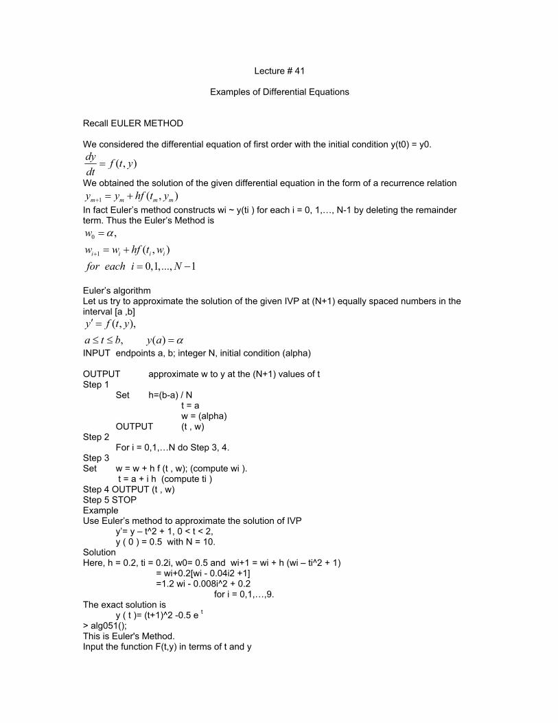
Lecture # 41
Examples of Differential Equations Recall EULER METHOD We considered the differential equation of first order with the initial condition y(t0) = y0.
( , )dy
f t ydt
We obtained the solution of the given differential equation in the form of a recurrence relation
1 ( , )m m m my y hf t y! !
In fact Euler’s method constructs wi ~ y(ti ) for each i = 0, 1,…, N-1 by deleting the remainder term. Thus the Euler’s Method is
0
1
,
( , )
0,1,..., 1
i i i i
w
w w hf t w
for each i N
"
!
!
#
Euler’s algorithm Let us try to approximate the solution of the given IVP at (N+1) equally spaced numbers in the interval [a ,b]
( , ),
, ( )
y f t y
a t b y a "
$
% %
INPUT endpoints a, b; integer N, initial condition (alpha) OUTPUT approximate w to y at the (N+1) values of t Step 1 Set h=(b-a) / N t = a w = (alpha) OUTPUT (t , w) Step 2 For i = 0,1,…N do Step 3, 4. Step 3 Set w = w + h f (t , w); (compute wi ). t = a + i h (compute ti ) Step 4 OUTPUT (t , w) Step 5 STOP Example Use Euler’s method to approximate the solution of IVP y’= y – t^2 + 1, 0 < t < 2, y ( 0 ) = 0.5 with N = 10. Solution Here, h = 0.2, ti = 0.2i, w0= 0.5 and wi+1 = wi + h (wi – ti^2 + 1) = wi+0.2[wi - 0.04i2 +1] =1.2 wi - 0.008i^2 + 0.2 for i = 0,1,…,9. The exact solution is y ( t )= (t+1)^2 -0.5 e
t
> alg051(); This is Euler's Method. Input the function F(t,y) in terms of t and y

For example: y-t^2+1 > y-t^2+1 Input left and right endpoints separated by blank > 0 2 Input the initial condition > 0.5 Input a positive integer for the number of subintervals > 10 Choice of output method: 1. Output to screen 2. Output to text file Please enter 1 or 2 > 1 Output t w 0.000 0.5000000 0.200 0.8000000 0.400 1.1520000 0.600 1.5504000 0.800 1.9884800 1.000 2.4581760 > alg051(); This is Euler's Method. Input the function F (t,y) in terms of t and y For example: y-3*t^2+4 > y-3*t^2+4 Input left and right hand points separated by a blank >0 1 Input the initial condition > 0.5 Input a positive integer for the number of subintervals > 10 Choice of output method: 1. Output to screen 2. Output to text file Please enter 1 or 2 > 1 Output t w 0.000 0.5000000 0.100 0.9500000 0.200 1.4420000 0.300 1.9742000 0.400 2.5446200 0.500 3.1510820 0.600 3.7911902 0.700 4.4623092 0.800 5.1615401 0.900 5.8856942 1.000 6.6312636 Recall Runge-Kutta (Order Four) METHOD The fourth-order R-K method was described as
1 1 2 3 4
1( 2 2 )6
n ny y k k k k! ! ! ! !
where

1
12
23
4 3
( , )
,2 2
,2 2
( , )
n n
n n
n n
n n
k hf t y
khk hf t y
khk hf t y
k hf t h y k
& ' ! !( )
* +
& ' ! !( )
* +
! !
Example Solve the following differential equation
dyt y
dt ! with the initial condition y(0) = 1, using fourth- order Runge-Kutta method from t = 0
to t = 0.4 taking h = 0.1 Solution The fourth-order Runge-Kutta method is described as
1 1 2 3 4
1( 2 2 ) ..................(1)6
n ny y k k k k! ! ! ! !
where
1
12
23
4 3
( , )
,2 2
,2 2
( , )
n n
n n
n n
n n
k hf t y
khk hf t y
khk hf t y
k hf t h y k
& ' ! !( )
* +
& ' ! !( )
* +
! !
In this problem,
0 0( , ) , 0.1, 0, 1.f t y t y h t y !
As a first step, we calculate
1 0 0
2 0 0
3 0 0
4
( , ) 0.1(1) 0.1
( 0.05, 0.05)
(0.05,1.05) 0.1[0.05 1.05]
0.11
( 0.05, 0.055)
0.1(0.05 1.055)
0.1105
0.1(0.1 1.1105) 0.12105
k hf t y
k hf t y
hf
k hf t y
k
! !
!
! !
!
!
Now, we compute from

1 0 1 2 3 4
1( 2 2 )6
11 (0.1 0.22 0.2210 0.12105)6
1.11034
y y k k k k ! ! ! !
! ! ! !
Therefore y(0.1) = y1=1.1103 In the second step, we have to find y2 = y(0.2) We compute
1 1 1
12 1 1
23 1 1
4 1 1 3
( , ) 0.1(0.1 1.11034) 0.121034
,2 2
0.1[0.15 (1.11034 0.060517)] 0.13208
,2 2
0.1[0.15 (1.11034 0.06604)] 0.132638
( , )
0.1[0.2 (1.11034 0.13263
k hf t y
khk hf t y
khk hf t y
k hf t h y k
!
& ' ! !( )
* +
! !
& ' ! !( )
* +
! !
! !
! ! 8)] 0.1442978
From Equation (1), we see that
2
11.11034 [0.121034 2(0.13208)
6
2(0.132638) 0.1442978] 1.2428
y ! !
! !
Similarly we calculate,
1 2 2
12 2 2
23 1 1
4 2 2 3
( , ) 0.1[0.2 1.2428] 0.14428
, 0.1[0.25 (1.2428 0.07214)] 0.1564942 2
, 0.1[0.3 (1.2428 0.078247)] 0.15710472 2
( , ) 0.1[0.3 (1.2428 0.1571047)]
k hf t y
khk hf t y
khk hf t y
k hf t h y k
!
& ' ! ! ! ! ( )
* +
& ' ! ! ! ! ( )
* +
! ! ! ! 0.16999047
Using equation (1), we compute
3 2 1 2 3 4
1(0.3) ( 2 2 ) 1.399711
6y y y k k k k ! ! ! !
Finally, we calculate
1 3 3
12 3 3
23 3 3
4 3 3 3
( , ) 0.1[0.3 1.3997] 0.16997
, 0.1[0.35 (1.3997 0.084985)] 0.18346852 2
, 0.1[0.35 (1.3997 0.091734)] 0.18414342 2
( , ) 0.1[0.4 (1.3997 0.184143
k hf t y
khk hf t y
khk hf t y
k hf t h y k
!
& ' ! ! ! ! ( )
* +
& ' ! ! ! ! ( )
* +
! ! ! ! 4)] 0.19838434
Using them in equation (1), we get
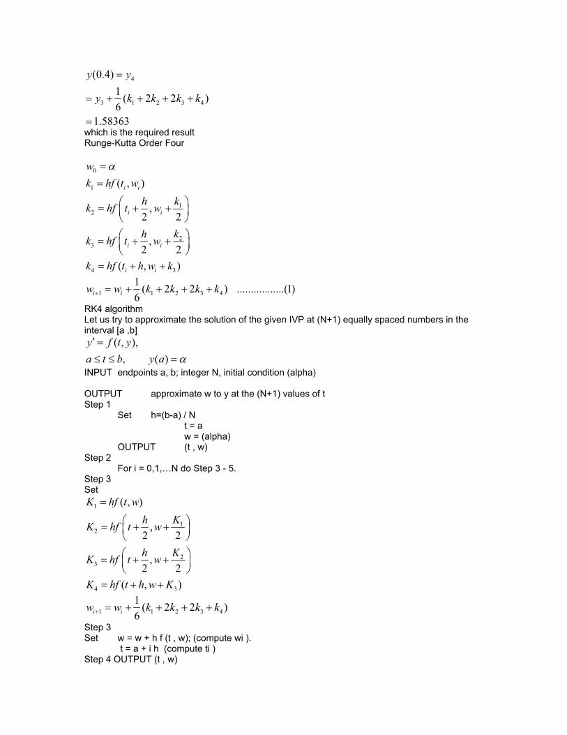
4
3 1 2 3 4
(0.4)
1( 2 2 )6
1.58363
y y
y k k k k
! ! ! !
which is the required result Runge-Kutta Order Four
0
1
12
23
4 3
( , )
,2 2
,2 2
( , )
i i
i i
i i
i i
w
k hf t w
khk hf t w
khk hf t w
k hf t h w k
"
& ' ! !( )
* +
& ' ! !( )
* +
! !
1 1 2 3 4
1( 2 2 ) .................(1)6
i iw w k k k k! ! ! ! !
RK4 algorithm Let us try to approximate the solution of the given IVP at (N+1) equally spaced numbers in the interval [a ,b]
( , ),
, ( )
y f t y
a t b y a "
$
% %
INPUT endpoints a, b; integer N, initial condition (alpha) OUTPUT approximate w to y at the (N+1) values of t Step 1 Set h=(b-a) / N t = a w = (alpha) OUTPUT (t , w) Step 2 For i = 0,1,…N do Step 3 - 5. Step 3 Set
1
12
23
4 3
( , )
,2 2
,2 2
( , )
K hf t w
KhK hf t w
KhK hf t w
K hf t h w K
& ' ! !( )
* +
& ' ! !( )
* +
! !
1 1 2 3 4
1( 2 2 )6
i iw w k k k k! ! ! ! !
Step 3 Set w = w + h f (t , w); (compute wi ). t = a + i h (compute ti ) Step 4 OUTPUT (t , w)

Step 5 STOP > alg052(); This is the Runge-Kutta Order Four Method. Input the function F(t,y) in terms of t and y For example: y-t^2+1 > y-t^2+1 Input left and right endpoints separated by blank > 0 2 Input the initial condition > 0.5 Input a positive integer for the number of subintervals > 10 Choice of output method: 1. Output to screen 2. Output to text file Please enter 1 or 2 > 1 Output t w 0.000 0.5000000 0.200 0.8292933 0.400 1.2140762 0.600 1.6489220 0.800 2.1272027 1.000 2.6408227 1.200 3.1798942 1.400 3.7323401 1.600 4.2834095 1.800 4.8150857 2.000 5.3053630

LLeeccttuurree 4422
Examples of Numerical Differentiation
The simplest formula for differentiation is
!2
(2)
0 0 0
1( ) ( ) ( ) ( ),
2
hf x f x h f x f
h"# $ % & &
Example Let f(x)= In x and x0 = 1.8. Then quotient
(1.8 ) (1.8), 0,
f h fh
h
% &'
is used to approximate (1.8)f # with error
2 2
( ),
2 2 2(1.8)
hf h h""
##$ ( where 1.8 1.8 .h") ) %
Let us see the results for h = 0.1, 0.01, and 0.001.
h f(1.8 + h)
(1.8 ) (1.8)f h f
h
% &
22(1.8)
h
0.1 0.64185389 0.5406722 0.0154321
0.01 0.59332685 0.5540180 0.0015432
0.001 0.58834207 0.5554013 0.0001543

Since ( ) 1/ ,f x x# $
The exact value of (1.8)f # is 0.555 and the error bounds are a appropriate.
The following two three point formulas become especially useful if the nodes are equally spaced, that is, when x1 = x0 + h and x2 = x0 + 2h,
!2
(3)
0 0 0 0 0
1( ) 3 ( ) 4 ( ) ( 2 ) ( ),
2 3
hf x f x f x h f x h f
h"# $ & % % & % %
where 0" lies between x0 and x0 + 2h, and
!2
(3)
0 0 0 1
1( ) ( ) ( ) ( ),
2 6
hf x f x h f x h f
h"# $ % & & &
where 1" lies between (x0 – h) and (x0 + h).
Given in Table below are values for f (x) = xex.
x f (x)
1.8 10.889365
1.9 12.703199
2.0 14.778112
2.1 17.148957
2.2 19.855030
Since
( ) ( 1) , (2.0) 22.167168.xf x x e f# #$ % $
Approximating (2.0)f #
using the various three-and five-point formulas produces the following results.
Three point formulas:
!2
(3)
0 0 0 0 0
1( ) 3 ( ) 4 ( ) ( 2 ) ( ),
2 3
hf x f x f x h f x h f
h"# $ & % % & % %
!2
(3)
0 0 0 1
1( ) ( ) ( ) ( ),
2 6
hf x f x h f x h f
h"# $ % & & &
Using three point formulas we get
!10.1: 3 (2.0) 4 (2.1) (2.2)
0.2
22.032310,
h f f f$ & % &
$

!10.1: 3 (2.0) 4 (1.9) (1.8)
0.2
22.0054525,
h f f f$ & & % &&
$
!10.1: (2.1) (1.9)
0.2
22.228790,
h f f$ &
$
!10.2 : (2.2) (1.8)
0.4
22.414163.
h f f$ &
$
Five point formula Using the five point formula with h = 0.1 (the only formula applicable):
!0 0 0 0 0
1( ) ( 2 ) 8 ( ) 8 ( ) ( 2 )
12f x f x h f x h f x h f x h
h# $ & & & % % & %
!1(1.8) 8 (1.9) 8 (2.1) (2.2)
0.2
22.166999.
f f f f$ & % &
$
The errors in the formulas are approximately
1 1 2 11.35 10 ,1.13 10 , 6.16 10 , 2.47 10 ,& & & &* * & * & *
and 41.69 10 ,&*
respectively. Clearly, the five-point formula gives the superior result. Consider approximating for f (x) = sin x, using the values in table [ the true value is cos (0.900) = 0.62161.]
x sin x x sin x
0.800 0.71736 0.901 0.78395
0.850 0.75128 0.902 0.78457
0.880 0.77074 0.905 0.78643
0.890 0.77707 0.910 0.78950
0.895 0.78021 0.920 0.79560
0.898 0.78208 0.950 0.81342
0.899 0.78270 1.000 0.84147
Using the formula

(0.900 ) (0.900 )(0.900)
2
f h f hf
h
% & &# +
with different values of h gives the approximations in table given below:
h Approximation to
(0.900)f #
Error
0.001 0.62500 0.00339
0.002 0.62250 0.00089
0.005 0.62200 0.00039
0.010 0.62150 -0.00011
0.020 0.62150 -0.00011
0.050 0.62140 -0.00021
0.100 0.62055 -0.00106

Examples of Numerical Integration EXAMPLE The Trapezoidal rule for a function f on the interval [0, 2] is
2
0 10
2
0
( ) [ ( ) ( )]2
( ) (0) (2),
hf x dx f x f x
f x dx f f
$ %
+ %
,
,
while Simpson’s rule for f on [0, 2] is
2
0 1 20
( ) [ ( ) 4 ( ) ( )].3
hf x dx f x f x f x$ % %,
That is
2
0
1( ) [ (0) 4 (1) (2)].
3f x dx f f f+ % %,
f (x) x2 x4 1/(x + 1)
21 x% sin x ex
Exact value 2.667 6.400 1.099 2.958 1.416 6.389
Trapezoidal 4.000 16.000 1.333 3.326 0.909 8.389
Simpson’s 2.667 6.667 1.111 2.964 1.425 6.421
Use close and open formulas listed below to approximate / 4
0sin 1 2 2xdx
-$ &,
Some of the common closed Newton-Cotes formulas with their error terms are as follows: n = 1: Trapezoidal rule
1
0
3
0 1( ) [ ( ) ( )] ( ),2 12
x
x
h hf x dx f x f x f "##$ % &,
Where 0 1.x x") )
n = 2: Simpson’s rule

2
0
5(4)
0 1 2 0 2( ) [ ( ) 4 ( ) ( )] ( ), .2 90
x
x
h hf x dx f x f x f x f x x" "$ % % & ) ),
n = 3: Simpson’s rule
3
0
5(4)
0 1 2 3
3 3( ) [ ( ) 3 ( ) 3 ( ) ( )] ( ),
8 80
x
x
h hf x dx f x f x f x f x f "$ % % % &, 0 3.x x") )
n = 4:
1
2
7(6)
0 1 2 3 4
2 8( ) [7 ( ) 32 ( ) 12 ( ) 32 ( ) 7 ( )] (
45 945
x
x
h hf x dx f x f x f x f x f x f "$ % % % % &,
Where 0 4.x x") )
n = 0: Midpoint rule
1
2
3
0( ) 2 ( ) ( ),3
x
x
hf x dx hf x f "##$ %, where 1 1.x x"& ) )
n 1 2 3 4
Closed formulas
0.27768018 0.29293264 0.29291070 0.29289318
Error 0.01521303 0.00003942 0.00001748 0.00000004
Open formulas 0.29798754 0.29285866 0.29286923
Error 0.00509432 0.00003456 0.00002399
Composite Numerical Integration

EXAMPLE 1
Consider approximating 0
sin xdx-
, with an absolute error less than 0.00002, using the
Composite Simpson’s rule. The Composite Simpson’s rule gives 4( / 2) 1 / 2
2 2 10
1 1
sin 2 sin 4 sin sin .3 180
n n
j j
j j
h hxdx x x
- -.
&
&$ $
/ 0$ % &1 2
3 45 5,
Since the absolute error is required to be less than 0.00002, the inequality 4 4 5
4sin 0.00002
180 180 180
h h
n
- - -. ( $ )
is used to determine n and h. Computing these calculations gives n greater than or equal to 18. If n = 20, then the formula becomes
9 10
01 1
(2 1)sin 2 sin 4 sin 2.000006.
60 10 20j j
j jxdx
- - - -
$ $
/ 0&6 7 6 7+ % $1 28 9 8 9: ; : ;3 4
5 5,
To be assured of this degree of accuracy using the Composite Trapezoidal rule requires that
2 2 3
2sin 0.00002
12 12 12
h h
n
- - -. ( $ )
or that 360.n < Since this is many more
calculations than are needed for the Composite Simpson’s rule, it is clear that it would be undesirable to use the Composite Trapezoidal rule on this problem. For comparison purposes, the Composite Trapezoidal rule with n = 20 and gives
19
01
19
1
sin 2 sin sin 0 sin40 20
2 sin 1.9958860.40 20
j
j
jxdx
j
- - --
- -
$
$
/ 06 7+ % %1 28 9: ;3 4
/ 06 7$ $1 28 9: ;3 4
5,
5
The exact answer is 2; so Simpson’s rule with n = 20 gave an answer well within the required error bound, whereas the Trapezoidal rule with n = 20 clearly did not.
An Example of Industrial applications: A company advertises that every roll of toilet paper
has at least 250 sheets. The probability that there are 250 or more sheets in the toilet paper is given by
20.3881( 252.2)
250( 250) 0.3515 yP y e dy
= & &< $ ,
Approximating the above integral as 2270
0.3881( 252.2)
250( 250) 0.3515 yP y e dy& &< $ ,
a)use single segment Trapezoidal rule to find the probability that there are 250 or more sheets. b)Find the true error, Et for part (a). C)Find the absolute relative true error for part (a).

( ) ( )( )
2
f a f bI b a
%/ 0+ & 1 23 4 where
250a $ 270b $ 20.3881( 252.2)( ) 0.3515 yf y e& &$
20.3881(250 252.2)(250) 0.3515f e& &$
0.053721$ 20.3881(270 252.2)(270) 0.3515f e& &$
541.3888 10&$ *
540.053721 1.3888 10(270 250)
2I
&/ 0% *$ & 1 2
3 4
0.53721$
b) The exact value of the above integral cannot be found. We assume the value obtained by adaptive numerical integration using Maple as the exact value for calculating the true error and relative true error.
22700.3881( 252.2)
250( 250) 0.3515 yP y e dy& &< $ ,
0.97377$
so the true error is 0.97377 0.53721$ & 0.43656$
The absolute relative true error,
t> , would then be
True Error100
True Valuet> $ *
0.97377 0.53721100
0.97377
&$ *
44.832%$
Improper Integrals EXAMPLE To approximate the values of the improper integral
1
0,
xedxx
,
we will use the Composite Simpson’s rule with h = 0.25. Since the fourth Taylor polynomial for ex about x = 0 is
2 3 4
4 ( ) 1 .2 6 24
x x xP x x$ % % % %
We have 1
11 2 3 2 5 2 7 2 9 24
0 0
( ) 2 1 1 1lim 2
3 5 21 180MM
P xdx x x x x x
x%?
/ 0$ % % % %1 23 4,
2 1 1 12 2.9235450.
3 5 21 108$ % % % % +
Table below lists the approximate values of

4 ( )when 0 1
( ) 4when 0
0,
xe P xx
G xx
@ &) (A
$ B$A
C
x G(x)
0.00 0
0.25 0.0000170
0.50 0.0004013
0.75 0.0026026
1.00 0.0099485
Applying the Composite Simpson’s rule to G using these data gives
1
0( )
0.25[0 4(0.0000170) 2(0.0004013)
3
4(0.0026026) 0.0099485]
0.0017691
G x dx +
% %
% %
$
,
Hence
1
02.9235450 0.0017691 2.9253141.
xedxx
+ % $,
This result is accurate within the accuracy of the Composite Simpson’s rule approximation for the
function G. Since (4) ( ) 1G x )
on [0, 1], the error is bounded by
41 0
(0.25) (1) 0.0000217.180
&$
EXAMPLE To approximate the value of the improper integral
3 2
1
1sin .I x dxx
= &$ ,

we make the change of variable t = x-1
to obtain 1
1 2
0sin .I t t dt$ ,
The fourth Taylor polynomial, P4(t), for sin t about 0 is
3
4
1( ) ,
6P t t t$ &
So we have
311 11 2 5 26
1 20 0
sin 1
6
t t tI dt t t dt
t
& %$ % &, ,
13113 2 7 26
1 200
sin 2 1
3 21
t t tdt t t
t
& % / 0$ % &1 23 4,
3116
1 20
sin0.61904761.
t t tdt
t
& %$ %,
Applying the Composite Simpson’s rule with n = 8 to the remaining integral gives
0.0014890097 0.61904761 0.62053661,I $ % $
which is accurate to within 84.0 10 .&*

AAnn
IInnttrroodduuccttiioonn ttoo
MMAAPPLLEE
MMaappllee iiss aa ccoommpprreehheennssiivvee
ccoommppuutteerr ssyysstteemm ffoorr aaddvvaanncceedd mmaatthheemmaattiiccss..
IItt iinncclluuddeess ffaacciilliittiieess ffoorr iinntteerraaccttiivvee aallggeebbrraa,, ccaallccuulluuss,, ddiissccrreettee mmaatthheemmaattiiccss,, ggrraapphhiiccss,, nnuummeerriiccaall
ccoommppuuttaattiioonn eettcc..
IItt pprroovviiddeess aa uunniiqquuee eennvviirroonnmmeenntt ffoorr rraappiidd ddeevveellooppmmeenntt ooff mmaatthheemmaattiiccaall pprrooggrraammss uussiinngg iittss vvaasstt
lliibbrraarryy ooff bbuuiilltt--iinn ffuunnccttiioonnss aanndd ooppeerraattiioonnss.. Syntax :As with any computer language, Maple has its own syntax. We try to explain some of the symbols used in Maple
Symbol Description Examples Sample Output
; End-of-line. Tells Maple to process the line and show the output.
hello; hello
: End-of-line. Tells Maple to process the line and hide the output.
hello:
:= Assignment. Lets you assign values to variables.
a := 3; a;
a := 3 3
+, - Addition, subtraction. 1 + 3; 1 - 3;
4 -2
*, / Multiplication, division 3*412; 1236/3; 7/3;
1236 412 7/3
^, sqrt Power, square root 2^3; sqrt(2); 2^(1/2);
evalf, . Floating-point (decimal) evaluation evalf(7/3); 7.0/3;
2.333333333 2.333333333

I,Pi Imaginary unit, Pi. 2 + 3*I; (2*I)^2; evalf(Pi);
2+3I -4 3.14159265
%, %% Recall the last output, recall the second-to-last output, etc.
%; %%%;
3.14159265-4
Some syntactical Tips: Maple is case sensitive. foo, Foo, and FOO are three different things. x*y gives the product of x and y, xy is one variable To get the constant e use exp(1).
UUssiinngg tthhee %% ooppeerraattoorr ccaann ggiivvee ccoonnffuussiinngg rreessuullttss.. IItt aallwwaayyss rreettuurrnnss tthhee llaasstt oouuttppuutt ffrroomm tthhee
KKeerrnneell,, wwhhiicchh mmaayy hhaavvee nnootthhiinngg ttoo ddoo wwiitthh wwhheerree tthhee ccuurrssoorr iiss ((oorr wwhhiicchh wwoorrkksshheeeett iiss aaccttiivvee))..
IIff MMaappllee ddooeessnn''tt rreeccooggnniizzee ssoommeetthhiinngg,, iitt aassssuummeess iitt aass aa vvaarriiaabbllee;; ee..gg.. ttyyppiinngg ii^̂22 wwiillll ggiivvee yyoouu
ii22,,wwhhiillee wwee mmaayy bbee wwaanntteedd --11..
SSppaacceess aarree ooppttiioonnaall..
GGrreeeekk lleetttteerrss mmaayy bbee eenntteerreedd bbyy ssppeelllliinngg tthheeiirr nnaammee.. FFoorr eexxaammppllee,, aallpphhaa iiss aallwwaayyss ddiissppllaayyeedd
aass ,, aanndd GGaammmmaa iiss ddiissppllaayyeedd aass !
((nnoottee uuppppeerr--ccaassee)).. Built-in Data Capabilities Maple can handle arbitrary-precision floating point numbers. In other words, Maple can store as many digits for a number as you like, up to the physical limits of your computer's memory. To control this, use the Digits variable. sqrt(2.0); 1.414213562 Digits := 20: sqrt(2.0); 1.4142135623730950488
MMaappllee sseettss DDiiggiittss ttoo bbee 1100 bbyy ddeeffaauulltt.. YYoouu ccaann aallssoo tteemmppoorraarriillyy ggeett pprreecciissiioonn rreessuullttss bbyy ccaalllliinngg
eevvaallff wwiitthh aa sseeccoonndd aarrgguummeenntt..
eevvaallff((ssqqrrtt((22)),, 1155));;
11..4411442211335566223377331100
LLaarrggee iinntteeggeerrss aarree hhaannddlleedd aauuttoommaattiiccaallllyy
UUssiinngg ssyymmbboolliicc ccoommppuuttaattiioonn
TThhee mmaaiinn ffeeaattuurree ooff MMaappllee iiss ssyymmbboolliicc ccoommppuuttaattiioonn..

IInn ootthheerr wwoorrddss,, MMaappllee ddooeess aallggeebbrraa..
EExxaammppllee OOuuttppuutt CCoommmmeennttss
((xx ++ yy))^̂22;; ((xx ++ yy))22 AA bbaassiicc eexxpprreessssiioonn..
kk ::== xx**yy ++ yy^̂22;; kk ::== xxyy ++ yy22
kk iiss nnooww aann aalliiaass ffoorr tthhee eexxpprreessssiioonn.. NNoottee tthhaatt kk iiss
ssiimmppllyy aannootthheerr nnaammee ffoorr tthhee eexxpprreessssiioonn -- tthheeyy aarree nnoott
eeqquuaall iinn tthhee mmaatthheemmaattiiccaall sseennssee..
pp ::== kk //((xx++yy));; YYoouu ccaann nnooww uussee kk ttoo rreeffeerr ttoo tthhee eexxpprreessssiioonn.. MMaappllee
iimmmmeeddiiaatteellyy ssuubbssttiittuutteess tthhee vvaalluuee ooff kk..
k := 'k'; k You can unassign a variable by assigning it to its own
name in single quotes.

simplify(p); y The simplify command does algebraic simplification.
p := x^2 - 8*x +15;
p := x2 - 8x + 15
Maple doesn't mind if you re-use names. The old value is lost.
solve(p=3,x); 2,6
Use the solve command to solve equations. Note the use of the = sign. Here, it is used in a mathematical
sense. Maple will try different values for x until it finds all of them that make the mathematical statement x2 - 8x +
15 = 3 true.
dpdx := diff(p,x); dpdx := 2x - 8 The diff command differentiates an expression
with respect to a variable.
int(p,x);
The int command integrates an expression. Note that the constant of integration is left off.
BBaassiicc PPlloottttiinngg
MMaappllee ccaann pprroodduuccee ggrraapphhss vveerryy eeaassiillyy.. HHeerree aarree ssoommee eexxaammpplleess,, sshhoowwccaassiinngg tthhee bbaassiicc
ccaappaabbiilliittiieess..
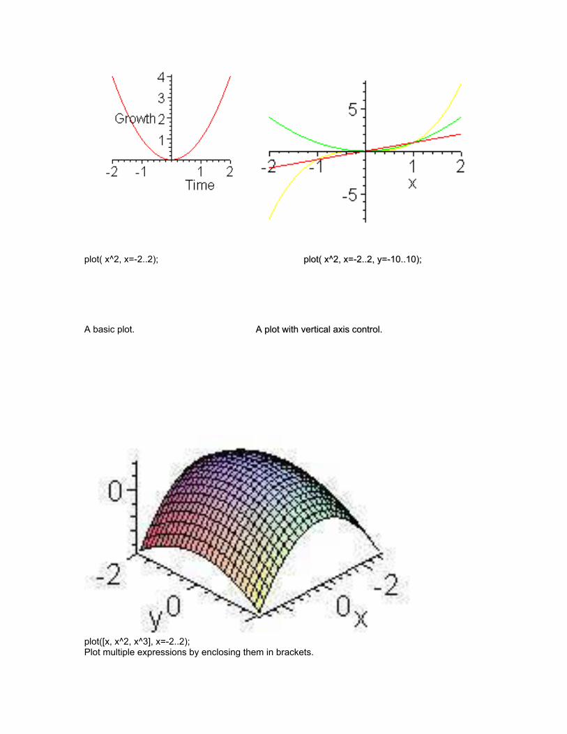
plot( x^2, x=-2..2); pplloott(( xx^̂22,, xx==--22....22,, yy==--1100....1100));;
A basic plot. AA pplloott wwiitthh vveerrttiiccaall aaxxiiss ccoonnttrrooll..
plot([x, x^2, x^3], x=-2..2); Plot multiple expressions by enclosing them in brackets.

plot3d(4-x^2-y^2, x=-3..3, y=-2..2);
A basic 3-d plot.
smartplot3d(x^2-y^2);

Using smartplot to let maple set it's own scaling.
EEiiggeennvvaallss aanndd vveeccttoorrss ooff aa nnuummeerriicc mmaattrriixx ::
CCaalllliinngg SSeeqquueennccee
EEiiggeennvvaallss(( AA,, vveeccss))
EEiiggeennvvaallss(( AA,, BB,, vveeccss))
PPaarraammeetteerrss
AA,,BB -- ssqquuaarree mmaattrriicceess ooff rreeaall oorr ccoommpplleexx nnuummbbeerrss
vveeccss -- ((ooppttiioonnaall)) nnaammee ttoo bbee aassssiiggnneedd tthhee mmaattrriixx ooff eeiiggeennvveeccttoorrss
Example
> A := array([[1,2,4],[3,7,2],[5,6,9]]);
evalf(Eigenvals(A));
> lambda := evalf(Eigenvals(A,vecs));
> print(vecs);
linalg[eigenvectors] - find the eigenvectors of a matrix
Calling Sequence
eigenvectors( A)
eigenvectors( A, 'radical')
eigenvectors( A, 'implicit')

Parameters
A - square matrix
The command with(linalg,eigenvectors) allows the use of the abbreviated form of this
command.
> with(linalg):
Warning, the protected names norm and trace have been redefined and unprotected
> A := matrix(3,3, [1,-3,3,3, -5,3,6,-6,4]);
> e := eigenvalues(A);
> v := [eigenvectors(A)];
> v[1][1]; # The first eigenvalue
4
> v[1][2]; # Its multiplicity
1
> v[1][3]; # Its eigenvectors
> v[2][1]; # The second eigenvalue
-2
> v[2][2]; # Its multiplicity
> v[2][2]; # Its multiplicity
2
Help
its worksheet interface
Waiting for command;
Restart; refresh memory;
# #; comments so no action implied
Eval - Evaluate an expression
Calling Sequence
Eval(a, x=n))
Eval(a, {x1=n1,x2=n2,...})
Parameters
a - an expression
x, x1, x2,... - names
n, n1, n2,... - evaluation points
Description
The Eval function is a place holder for evaluation at a point.
The expression a is evaluated at
x = n (x1=n1, x2=n2, ... for the multivariate case).

The call Eval (a, x=n) mod p evaluates the polynomial a at x=n modulo p .
Note: The polynomial must be a multivariate polynomial over a finite field.
The call modp1(Eval(a,n),p) evaluates the polynomial a at x = n modulo p where a
must be a univariate polynomial in the modp1 representation, with n an integer and p an
integer > 1.
Examples
Eval(x^2+1,x=3) mod 5;
0
Eval(x^2+y,{x=3,y=2}) mod 5;
> Eval (int (f(x),x), x=y);
Eigen values ?;
Solution of Problems
We can use Maple For:
Solution of non-linear equations
by Newton’s Method
by Bisection Method
Solution of System of linear equations.
Numerical Integration.
Numerical Solution of ODE’s.
Maple performs both numerical and symbolic itegration.
Please note that the Maple uses the int function for the both numerical and symbolic
integration, but for numerical integration we have to use the additional evalf command
Some inbuilt functions in Maple being used for integration
Numerical Integration
Calling Sequences
evalf(Int(f, x=a..b))
evalf(Int(f, a..b))
evalf(Int(f, x=a..b, opts))
evalf(Int(f, a..b, opts))
evalf(int(f, x=a..b))
We Define Parameters
f - algebraic expression or procedure; integrand
x - name; variable of integration
a,b - endpoints of the interval of integration
opts - (optional) name or equation of the form
option=name; options
Description
In the case of a definite integral, which is returned unevaluated, numerical integration
can be invoked by applying evalf to the unevaluated integral. To invoke numerical
integration without
first invoking symbolic integration, use the inert function Int as in: evalf( Int(f, x=a..b) ).
d"#$$
( )f x x%&%x y

If the integrand f is specified as a procedure or a Maple operator, then the second
argument must be the range a..b and not an equation. (i.e., a variable of integration must
not be specified.)
>evalf(Int( exp(-x^3), x = 0..1 ));.8075111821
>evalf(Int( exp(-x^3), x = 0..1 ));.8075111821
>evalf(Int( exp(-x^3), x = 0..1 ));8075111821
>alg041(); This is Simpson’s Method.
`Input the function F(x) in terms of x`
`For example:
> sin (x)
`Input lower limit of integration and upper limit of integration`
`separated by a blank`
> 0 3.14159265359
`Input an even positive integer N.`
> 20
The integral of F from 0.00000000
to
3.14159265
is 2.00000678
alg041(); This is Simpson’s Method.
`Input the function F(x) in terms of x`
> x^2
`Input lower limit of integration and upper limit of integration separated by a blank’
>0 2
Input an even positive integer N
>20
The integral of F from
0.00000000
to
2.00000000
is 2.66666667
> alg041();
This is Simpson’s Method.
Input the function F(x) in terms of x, for example: cos(x)
> exp(x-x^2/2)
Input lower limit of integration and upper limit of integration separated by a blank
> 0 3.14159265359
Input an even positive integer N.
> 20
The integral of F from
0.00000000
to
3.14159265

is 3.41046542
> alg044();
This is Simpson's Method for double integrals.
Input the functions F(X,Y), C(X), and D(X) in terms of x and y separated by a space.
For example: cos(x+y) x^3 x
> exp(y/x) x^3 x^2
Input lower limit of integration and upper limit of integration separated by a blank
> 0.1 0.5
Input two even positive integers N, M ; there will be N subintervals for outer integral and
M subintervals for inner integral - separate with blank
> 10 10
The double integral of F from
0.100 to 0.500
Is .03330546
obtained with
N := 10 and M := 10
> alg045();
`This is Gaussian Quadrature for double integrals.`
`Input the function F(x,y) in terms of x and y`
`For example: sqrt(x^2+y^2)`
> exp (y/x)
Input the functions C(x), and D(x) in terms of x separated by a space
For example: cos (x) sin (x)
> x^3 x^2
Input lower limit of integration and upper limit of integration separated by a blank space
>0.1 0.5
Input two integers M > 1 and N > 1. This implementation of Gaussian quadrature
requires both to be less than or equal to 5.
M is used for the outer integral and N for the inner integral - separated by a space.
> 5 5
The double integral of F from
0.1000 to 0.5000
is 3.3305566120e-02
Or 0.03305566120
obtained with
M = 5 and N = 5

Lecture 44
SSoolluuttiioonn ooff
NNoonn--LLiinneeaarr EEqquuaattiioonnss
BBiisseeccttiioonn MMeetthhoodd
RReegguullaa--FFaallssii MMeetthhoodd
MMeetthhoodd ooff iitteerraattiioonn
NNeewwttoonn -- RRaapphhssoonn MMeetthhoodd
MMuulllleerr’’ss MMeetthhoodd
GGrraaeeffffee’’ss RRoooott SSqquuaarriinngg MMeetthhoodd
NNeewwttoonn --RRaapphhssoonn MMeetthhoodd
An approximation to the root is given by
01 0
0
( )
( )
f xx x
f x !
"
Better and successive approximations x2, x3, …, xn to the root are obtained from
1
( )
( )
nn n
n
f xx x
f x# !
"
NN--RR FFoorrmmuullaa
NNeewwttoonn’’ss aallggoorriitthhmm To find a solution to f(x)=0 given an initial approximation p0 INPUT initial approximation p0; tolerance TOL; maximum number of iterations N0 OUTPUT approximate solution p or message of failure Step 1 Set I = 1 Step 2 While i < N0 do Steps 3-6 Step 3 Set p = p0 – f ( p0 ) / f’ ( p0 ) (compute pi ). Step 4 If Abs (p – p0) < TOL OUTPUT ( p ); (The procedure was successful.) STOP Step 5 Set i = i + 1 Step 6 Set p0 = p (Update p0 ) Step 7 OUTPUT (The method failed after N0 iterations, N0 = ‘,N0 ) The procedure was unsuccessful STOP
EExxaammppllee Using Maple to solve a non-linear equation.
cos( ) 0x x!

SSoolluuttiioonn The Maple command will be as follows, Fsolve ( cos (x) -x);
alg023(); This is Newton's Method
Input the function F(x) in terms of x For example: > cos(x)-x Input initial approximation > 0.7853981635 Input tolerance > 0.00005 Input maximum number of iterations - no decimal point > 25 Select output destination 1. Screen 2. Text file Enter 1 or 2 > 1 Select amount of output 1. Answer only 2. All intermediate approximations Enter 1 or 2 > 2
NNeewwttoonn''ss MMeetthhoodd I P F(P) 1 0.739536134 -7.5487470e-04 2 0.739085178 -7.5100000e-08 3 0.739085133 0.0000000e-01 Approximate solution = 0.73908513 with F(P) = 0.0000000000 Number of iterations = 3 Tolerance = 5.0000000000e-05
AAnnootthheerr EExxaammppllee > alg023(); Input the function F(x) in terms of x , > sin(x)-1 Input initial approximation > 0.17853 Input tolerance > 0.00005 Input maximum number of iterations – no decimal point > 25 Select output destination 1. Screen 2. Text file Enter 1 or 2 >2 Select amount of output 1. Answer only 2. All intermediate approximations Enter 1 or 2 > 2
NNeewwttoonn''ss MMeetthhoodd

I P F(P) 1 1.01422964e+00 -1.5092616e-01 2 1.29992628e+00 -3.6461537e-02 3 1.43619550e+00 -9.0450225e-03 4 1.50359771e+00 -2.2569777e-03 5 1.53720967e+00 -5.6397880e-04 6 1.55400458e+00 -1.4097820e-04 7 1.56240065e+00 -3.5243500e-05 More… 8 1.56659852e+00 -8.8108000e-06 9 1.56869743e+00 -2.2027000e-06 10 1.56974688e+00 -5.5070000e-07 11 1.57027163e+00 -1.3770000e-07 12 1.57053407e+00 -3.4400000e-08 13 1.57066524e+00 -8.6000000e-09 14 1.57073085e+00 -2.1000000e-09 15 1.57076292e+00 -6.0000000e-10 Approximate solution = 1.57076292 with F(P) =6.0000000000e-10 Number of iterations = 15 Tolerance = 5.0000000000e-05
BBiisseeccttiioonn MMeetthhoodd
> alg021(); This is the Bisection Method. Input the function F(x) in terms of x For example: > x^3+4*x^2-10 Input endpoints A < B separated by blank > 1 2 Input tolerance > 0.0005 Input maximum number of iterations - no decimal point > 25 Select output destination
1. Screen , 2. Text file Enter 1 or 2 > 1 Select amount of output 1. Answer only 2. All intermediate approximations Enter 1 or 2 > 2
BBiisseeccttiioonn MMeetthhoodd I P F(P) 1 1.50000000e+00 2.3750000e+00 2 1.25000000e+00 -1.7968750e+00 3 1.37500000e+00 1.6210938e-01 4 1.31250000e+00 -8.4838867e-01 5 1.34375000e+00 -3.5098267e-01 6 1.35937500e+00 -9.6408842e-02

7 1.36718750e+00 3.2355780e-02 8 1.36328125e+00 -3.2149969e-02 9 1.36523438e+00 7.2030000e-05 10 1.36425781e+00 -1.6046697e-02 11 1.36474609e+00 -7.9892590e-03 Approximate solution P = 1.36474609 with F(P) = -.00798926 Number of iterations = 11 Tolerance = 5.00000000e-04 alg021(); Another example of the Bisection Method. Input the function F(x) in terms of x, > cos(x) Input endpoints A < B separated by blank > 1 2 Input tolerance > 0.0005 Input maximum number of iterations - no decimal point > 25 Select output destination 1. Screen , 2. Text file Enter 1 or 2 > 1 Select amount of output 1. Answer only 2. All intermediate approximations Enter 1 or 2 > 2
BBiisseeccttiioonn MMeetthhoodd 1 P F(P) 1 1.50000000e+00 7.0737202e-02 2 1.75000000e+00 -1.7824606e-01 3 1.62500000e+00 -5.4177135e-02 4 1.56250000e+00 8.2962316e-03 5 1.59375000e+00 -2.2951658e-02 6 1.57812500e+00 -7.3286076e-03 7 1.57031250e+00 4.8382678e-04 8 1.57421875e+00 -3.4224165e-03 9 1.57226563e+00 -1.4692977e-03 10 1.57128906e+00 -4.9273519e-04 11 1.57080078e+00 -4.4542051e-06 Approximate solution P = 1.57080078 with F(P) = -.00000445 Number of iterations = 11 Tolerance = 5.00000000e-04
alg025(); This is the Method of False Position Input the function F(x) in terms of x > cos(x)-x Input endpoints P0 < P1 separated by a blank space
0.5 0.7853981635 Input tolerance >0.0005 Input maximum number of iterations - no decimal point > 25

Select output destination 1. Screen 2. Text file Enter 1 or 2 >1 Select amount of output 1. Answer only 2. All intermediate approximations Enter 1 or 2 > 2
MMEETTHHOODD OOFF FFAALLSSEE PPOOSSIITTIIOONN I P F(P) 2 7.36384139e-01 4.51771860e-03 3 7.39058139e-01 4.51772000e-05 4 7.39084864e-01 4.50900000e-07 Approximate solution P = .73908486 with F(P) = .00000045 Number of iterations = 4 Tolerance = 5.00000000e-04
SSyysstteemm ooff LLiinneeaarr EEqquuaattiioonnss
GGaauussssiiaann EElliimmiinnaattiioonn GGaauussss--JJoorrddoonn EElliimmiinnaattiioonn
CCrroouutt’’ss RReedduuccttiioonn JJaaccoobbii’’ss
GGaauussss-- SSeeiiddaall IItteerraattiioonn RReellaaxxaattiioonn
MMaattrriixx IInnvveerrssiioonn > alg061(); This is Gaussian Elimination to solve a linear system. The array will be input from a text file in the order: A(1,1), A(1,2), ..., A(1,N+1), A(2,1), A(2,2), ..., A(2,N+1),..., A(N,1), A(N,2), ..., A(N,N+1) Place as many entries as desired on each line, but separate entries with at least one blank. Has the input file been created? - enter Y or N. > y Input the file name in the form - drive:\name.ext for example: A:\DATA.DTA > d:\maple00\dta\alg061.dta Input the number of equations - an integer. > 4 Choice of output method: 1. Output to screen 2. Output to text file Please enter 1 or 2. > 1
GGAAUUSSSSIIAANN EELLIIMMIINNAATTIIOONN The reduced system - output by rows: 1.00000000 -1.00000000 2.00000000 -1.00000000 -8.00000000 0.00000000 2.00000000 -1.00000000 1.00000000 6.00000000 0.00000000 0.00000000 -1.00000000 -1.00000000 -4.00000000 0.00000000 0.00000000 0.00000000 2.00000000 4.00000000 Has solution vector: -7.00000000 3.00000000 2.00000000 2.00000000

with 1 row interchange (s) > alg071(); This is the Jacobi Method for Linear Systems. The array will be input from a text file in the order A(1,1), A(1,2), ..., A(1,n+1), A(2,1), A(2,2), ..., A(2,n+1),..., A(n,1), A(n,2), ..., A(n,n+1) Place as many entries as desired on each line, but separate entries with at least one blank. The initial approximation should follow in the same format has the input file been created? - enter Y or N. > y Input the file name in the form - drive:\name.ext for example: A:\DATA.DTA > d:\maple00\alg071.dta Input the number of equations - an integer. > 4 Input the tolerance. > 0.001 Input maximum number of iterations. > 15 Choice of output method: 1. Output to screen 2. Output to text file Please enter 1 or 2. > 1
JJAACCOOBBII IITTEERRAATTIIVVEE MMEETTHHOODD FFOORR LLIINNEEAARR SSYYSSTTEEMMSS
The solution vector is : 1.00011860 1.99976795 -.99982814 0.99978598 using 10 iterations with Tolerance 1.0000000000e-03
AAnn aapppprrooxxiimmaattiioonn ttoo tthhee rroooott iiss ggiivveenn bbyy
BBeetttteerr aanndd ssuucccceessssiivvee aapppprrooxxiimmaattiioonnss xx22,, xx33,, ……,, xxnn ttoo tthhee rroooott aarree oobbttaaiinneedd ffrroomm
EExxaammppllee
UUssiinngg MMaappllee ttoo ssoollvvee aa nnoonn--lliinneeaarr eeqquuaattiioonn..

SSyysstteemm ooff LLiinneeaarr EEqquuaattiioonnss
IInnppuutt tthhee ttoolleerraannccee..
>> 00..000011
IInnppuutt mmaaxxiimmuumm nnuummbbeerr ooff iitteerraattiioonnss..
>> 1155
CChhooiiccee ooff oouuttppuutt mmeetthhoodd::
11.. OOuuttppuutt ttoo ssccrreeeenn
22.. OOuuttppuutt ttoo tteexxtt ffiillee
PPlleeaassee eenntteerr 11 oorr 22..
>> 11

SSuummmmiinngg uupp
NNoonn--LLiinneeaarr
EEqquuaattiioonnss
BBiisseeccttiioonn MMeetthhoodd ((BBoollzzaannoo))
RReegguullaa--FFaallssii MMeetthhoodd
MMeetthhoodd ooff iitteerraattiioonn
NNeewwttoonn -- RRaapphhssoonn MMeetthhoodd
MMuulllleerr’’ss MMeetthhoodd
GGrraaeeffffee’’ss RRoooott SSqquuaarriinngg MMeetthhoodd
In the method of False Position, the first approximation to the root of f (x) = 0 is given by
11
1
( )( ) ( )
n nn n n
n n
x xx x f x
f x f x
!
"
………..(2.2)
Here f (xn-1) and f (xn+1) are of opposite sign. Successive approximations to the root of f (x) = 0 is given by Eq. (2.2).
METHOD OF ITERATION can be applied to find a real root of the equation f (x)
= 0 by rewriting the same in the form,, ( )x x#"
1 0
2 1
1
( )
( )
( )n n
x x
x x
x x
#
#
#!
" $%" %&%%" '
In Newton – Raphson Method successive approximations x2, x3, …, xn to the root are obtained from
1
( )
( )
nn n
n
f xx x
f x! "
(
N-R Formula

1 11
1
( ) ( ), 12,3
( ) ( )
n n n nn
n n
x f x x f xx n
f x f x
!
" "
!
This sequence converges to the root ‘b’ of f (x) = 0 i.e. f( b ) = 0.
The Secant method converges faster than linear and slower than Newton’s quadratic. In Muller’s Method we can get a better approximation to the root, by using
1i i ix x h)! " !
2 1/ 2
2 1
2
[ 4 ( )]
i i
i i i i i i i i i i
f
g g f f f f
*)
* ) ) *
"
+ !
Where we defined
1
1
1
i
i i i
ii
i
i i
x xh
h x x
h
h
)
)
* )
" "
"
" !
SSyysstteemmss ooff LLiinneeaarr
EEqquuaattiioonnss
GGaauussssiiaann EElliimmiinnaattiioonn GGaauussss--JJoorrddoonn EElliimmiinnaattiioonn
CCrroouutt’’ss RReedduuccttiioonn JJaaccoobbii’’ss
GGaauussss-- SSeeiiddaall IItteerraattiioonn RReellaaxxaattiioonn
MMaattrriixx IInnvveerrssiioonn
In Gaussian Elimination method, the solution to the system of equations is obtained in two stages.
• the given system of equations is reduced to an equivalent upper triangular form using elementary transformations
• the upper triangular system is solved using back substitution procedure
Gauss-Jordon method is a variation of Gaussian method. In this method, the elements above and below the diagonal are simultaneously made zero In Crout’s Reduction Method the coefficient matrix [A] of the system of equations is decomposed into the product of two matrices [L] and [U], where [L] is a lower-

triangular matrix and [U] is an upper-triangular matrix with 1’s on its main diagonal. For the purpose of illustration, consider a general matrix in the form
, -, - , -L U A"
11 12 13 11 12 13
21 22 23 21 22 23
31 32 33 31 32 33
0 0 1
0 0 1
0 0 1
l u u a a a
l l u a a a
l l l a a a
. / . / . /0 1 0 1 0 1"0 1 0 1 0 10 1 0 1 0 12 3 2 3 2 3
Jacobi’s Method is an iterative method, where initial approximate solution to a given system of equations is assumed and is improved towards the exact solution in an iterative way. In Jacobi’s method, the (r + 1)th approximation to the above system is given by Equations
( 1) ( ) ( )11 121 2
11 11 11
( 1) ( ) ( )22 212 1
22 22 22
( 1)( 1) ( ) ( )11 1
r r rnn
r r rnn
n nr r rn nn n
nn nn nn
ab ax x x
a a a
ab ax x x
a a a
ab ax x x
a a a
!
!
!
$" %%%
" %&%%%
" %'
"
"
"
Here we can observe that no element of ( 1)r
ix!
replaces ( )r
ix entirely for the next cycle of computation.
In Gauss-Seidel method, the corresponding elements of ( 1)r
ix!
replaces
those of ( )r
ix as soon as they become available. It is also called method of Successive Displacement.
The Relaxation Method is also an iterative method and is due to Southwell.
ii
ii
Rdx
a"
EEiiggeenn VVaalluuee PPrroobblleemmss

PPoowweerr MMeetthhoodd
JJccoobbii’’ss MMeetthhoodd In Power Method the result looks like
( ) ( 1) ( )[ ]k k k
ku A v q v " "
Here, kq is the desired largest eigen value and ( )kv is the corresponding
eigenvector.
IInntteerrppoollaattiioonn
FFiinniittee DDiiffffeerreennccee OOppeerraattoorrss
NNeewwttoonn’’ss FFoorrwwaarrdd DDiiffffeerreennccee IInntteerrppoollaattiioonn FFoorrmmuullaa
NNeewwttoonn’’ss BBaacckkwwaarrdd DDiiffffeerreennccee IInntteerrppoollaattiioonn FFoorrmmuullaa
LLaaggrraannggee’’ss IInntteerrppoollaattiioonn FFoorrmmuullaa
DDiivviiddeedd DDiiffffeerreenncceess
IInntteerrppoollaattiioonn iinn TTwwoo DDiimmeennssiioonnss
CCuubbiicc SSpplliinnee IInntteerrppoollaattiioonn
FFiinniittee DDiiffffeerreennccee OOppeerraattoorrss
FFoorrwwaarrdd DDiiffffeerreenncceess
BBaacckkwwaarrdd DDiiffffeerreenncceess
CCeennttrraall DDiiffffeerreennccee 1 1
1
1 1
1
1 1
(1 2) (1 2)
,
, ( 1),...,
r r r
i i i
k k k
i i i
n n n
i i i
y y y
y y y
i n n k
y y y* * *
!
!
4 " 4 4
5 " 5 5
"
"
Thus
2
( ) ( )x x h x
x x h x
y y y f x h f x
y y y
!
!
4 " " !
4 " 4 4
Similarly

( / 2) ( / 2)
( ) ( )
2 2
x x x h
x x h x h
y y y f x f x h
h hy y y f x f x*
!
5 " "
6 7 6 7" " ! 8 9 8 9: ; : ;
Shift operator, E
( ) ( )E f x f x h" !
( ) ( )nE f x f x nh" ! n
x x nhE y y !"
The inverse operator E-1 is defined as 1 ( ) ( )E f x f x h "
Similarly,
( ) ( )nE f x f x nh "
Average Operator, <
( / 2) ( / 2)
1( )
2 2 2
1
2x h x h
h hf x f x f x
y y
<
!
. /6 7 6 7" ! ! 8 9 8 90 1: ; : ;2 3
. /" !2 3
Differential Operator, D
22
2
( ) ( ) ( )
( ) ( ) ( )n
dDf x f x f x
dx
dD f x f x f x
dx
$(" " %%&%" "%'
Important Results
1E4 "
1 11
EE
E
5 " "
1/ 2 1/ 2E E* "
loghD E"
1/ 2 1/ 21( )
2E E< " !
The Newton’s forward difference formula for interpolation, which gives the value of f (x0 + ph) in terms of f (x0) and its leading differences.
0 0 0
2 3
0 0
0
( ) ( ) ( )
( 1) ( 1)( 2)( ) ( )
2! 3!
( 1) ( 1)( ) Error
!
n
f x ph f x p f x
p p p p pf x f x
p p p nf x
n
! " ! 4
! 4 ! 4
!! ! 4 !
""

An alternate expression is
2
0 0 0
3
0
0
( 1)
2!
( 1)( 2)
3!
( 1) ( 1)Error
!
x
n
p py y p y y
p p py
p p p ny
n
" ! 4 ! 4
! 4 !
!! 4 !
"
"
Newton’s Backward difference formula is,
2
3
( ) ( ) ( )
( 1)( )
2!
( 1)( 2)( )
3!
( 1)( 2) ( 1)( ) Error
!
n n n
n
n
n
n
f x ph f x p f x
p pf x
p p pf x
p p p p nf x
n
! " ! 5
!! 5
! !! 5 !
! ! ! ! 5 !
"
"
Alternatively, this formula can also be written as
2
3
( 1)
2!
( 1)( 2)
3!
( 1)( 2) ( 1)Error
!
x n n n
n
n
n
p py y p y y
p p py
p p p p ny
n
!" ! 5 ! 5
! !! 5 !
! ! ! ! 5 !
"
"
Here
nx xp
h
"
The Lagrange’s formula for interpolation
1 2 0 20 1
0 1 0 2 0 1 0 1 2 1
0 1 1 1 0 1 2
0 1 1 1
( )( ) ( ) ( )( ) ( )( )
( )( ) ( ) ( )( ) ( )
( )( ) ( )( ) ( ) ( )( )( ) (
( )( ) ( )( ) ( )
n n
n n
i i ni
i i i i i i i n
x x x x x x x x x x x xy f x y y
x x x x x x x x x x x x
x x x x x x x x x x x x x x x x xy
x x x x x x x x x x
!
!
" " ! !
! ! !
" ""
" "
" " ""
" "
1
0 1 2 1
)
( )( )( ) ( )
nn
n n n n n
xy
x x x x x x x x
"
Newton’s divided difference interpolation formula can be written as
0 0 0 1
0 1 0 1 2
0 1 1 0 1
( ) ( ) [ , ]
( )( ) [ , , ]
( )( ) ( ) [ , ,..., ]n n
y f x y x x y x x
x x x x y x x x
x x x x x x y x x x
" " !
!
! !
"
!
Where the first order divided difference is defined as

1 00 1
1 0
[ , ]y y
y x xx x
"
NNuummeerriiccaall DDiiffffeerreennttiiaattiioonn aanndd IInntteeggrraattiioonn We expressed D in terms of :
2 3 4 51
2 3 4 5D
h
6 74 4 4 4" 4 ! ! 8 9
: ;"
Using backward difference operator , we have log(1 ).hD " 5
On expansion, we have 2 3 41
2 3 4D
h
6 75 5 5" 5 ! ! !8 9
: ;"
Using Central difference Operator
3 51 1 3
24 640D
h* * *6 7" ! 8 9: ;
"
Differentiation Using Interpolation Richardson’s Extrapolation
1
0
10 1
0
( )
( )( ) ( )
n
i
i
nn
i i
dx x
dx
x x x x x x
x x
"
"
"
=
>"
Thus, ( )y x( is approximated by ( )nP x(
which is given by
0 1 1 0 0 1 2
10 1 1
0 1
0
( ) [ , ] [( ) ( )] [ , , ]
( )( ) ( )[ , , , ]
n
nn
n
i i
P x y x x x x x x y x x x
x x x x x xy x x x
x x
"
"
( " ! ! !
!
>
"
"!
1 1 1
2
42 2
,4 1
1, 2,3,
m m
m
m mm m
m
hF
h hF F
m
6 78 9: ;
6 7 6 7 8 9 8 9: ; : ;"
"
Basic Issues in Integration What does an integral represent? b
a
f (x)dx? = AREA

d b
c a
g(x, y) dx dy? ? = VOLUME
3
0
5 ( )
0 1 2 3
( )
3 3 ( 3 3 ) h ( )
8 80
x
x
iv
f x dx
h y y y y y @" ! ! !
?
yn-1y3y2y1 y0 yn
xn = bxn-1x3 x2 x1 x0 = a X O
Y
(x2, y2)(x1, y1)
(x0, y0)
y = f(x)

TTRRAAPPEEZZOOIIDDAALL RRUULLEE
0
0 1 2 1
( )
( 2 2 2 )2
nx
x
n n n
f x dx
hy y y y y E ! " " " " " "
#
DOUBLE INTEGRATION We described procedure to evaluate numerically a double integral of the form
( , )I x y dx dy$ %! & '# #
DDiiffffeerreennttiiaall EEqquuaattiioonnss
TTaayylloorr SSeerriieess
EEuulleerr MMeetthhoodd
RRuunnggee--KKuuttttaa MMeetthhoodd
PPrreeddiiccttoorr CCoorrrreeccttoorr MMeetthhoodd
xn = bxn-1x3 x2 x1 x0 = a X O
Y
(x2, y2)
(x0, y0)
y2y1 y0
y = f(x)

In Taylor’s series we expanded y (t ) by Taylor’s series about the point t = t0 and obtain
2 3 4
0 0 00 0 0 0 0 0
( ) ( ) ( )( ) ( ) ( ) ( ) ( ) ( ) ( )
2! 3! 4!
IVt t t t t ty t y t t t y t y t y t y t
( (( (((! " " " " "
In Euler Method we obtained the solution of the differential equation in the form of a recurrence relation
1 ( , )m m m my y hf t y" ! " We derived the recurrence relation
(1)
1 11
( , ) ( , )
2
m m m mm m
f t y f t yy y h " "
"
$ %"! " ) *
& '
Which is the modified Euler’s method. The fourth-order R-K method was described as
1 1 2 3 4
1( 2 2 )
6n ny y k k k k" ! " " " "
where
1
12
23
4 3
( , )
,2 2
,2 2
( , )
n n
n n
n n
n n
k hf t y
khk hf t y
khk hf t y
k hf t h y k
!
+ ,! " "- ./ 0
+ ,! " "- ./ 0
! " "
In general, Milne’s predictor-corrector pair can be written as
1 3 2 1
1 1 1 1
4: (2 2 )
3
: ( 4 )3
n n n n n
n n n n n
hP y y y y y
hC y y y y y
"
" "
1( ( (! " " 2232( ( (! " " "24
This is known as Adam’s predictor formula.
4
1 1 2 3
251(55 59 37 9 )
24 720n n n n n n n
hy y f f f f h f" ! " " " 5
Alternatively, it can be written as
6 7 4
1 1 2 3
25155 59 37 9
24 720n n n n n n n
hy y y y y y h y" ( ( ( ( (! " " " 5