numerical analysis and computingjmahaffy.sdsu.edu/courses/s10/math541/lectures/pdf/... ·...
TRANSCRIPT

Numerical Analysis and Computing
Lecture Notes #10— Approximation Theory —
Discrete Least Squares Approximation
Joe Mahaffy,〈[email protected]〉
Department of MathematicsDynamical Systems Group
Computational Sciences Research Center
San Diego State UniversitySan Diego, CA 92182-7720
http://www-rohan.sdsu.edu/∼jmahaffy
Spring 2010
Joe Mahaffy, 〈[email protected]〉 Discrete Least Squares Approximation — (1/33)
Outline
1 Approximation Theory: Discrete Least SquaresIntroductionDiscrete Least Squares
2 Discrete Least SquaresA Simple, Powerful Approach
3 Discrete Least SquaresApplication: Cricket Thermometer
Joe Mahaffy, 〈[email protected]〉 Discrete Least Squares Approximation — (2/33)
Approximation Theory: Discrete Least SquaresDiscrete Least Squares
IntroductionDiscrete Least Squares
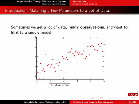
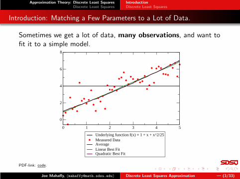
Introduction: Matching a Few Parameters to a Lot of Data.
Sometimes we get a lot of data, many observations, and want tofit it to a simple model.
0 1 2 3 4 5
0
2
4
6
8
Measured Data
Joe Mahaffy, 〈[email protected]〉 Discrete Least Squares Approximation — (3/33)

Approximation Theory: Discrete Least SquaresDiscrete Least Squares
IntroductionDiscrete Least Squares
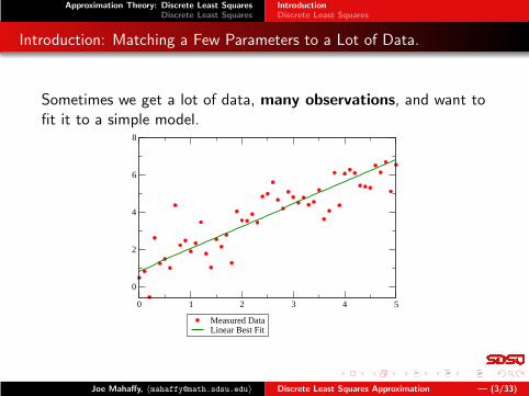
Introduction: Matching a Few Parameters to a Lot of Data.
Sometimes we get a lot of data, many observations, and want tofit it to a simple model.
0 1 2 3 4 5
0
2
4
6
8
Measured DataAverage
Joe Mahaffy, 〈[email protected]〉 Discrete Least Squares Approximation — (3/33)
Approximation Theory: Discrete Least SquaresDiscrete Least Squares
IntroductionDiscrete Least Squares
Introduction: Matching a Few Parameters to a Lot of Data.
Sometimes we get a lot of data, many observations, and want tofit it to a simple model.
0 1 2 3 4 5
0
2
4
6
8
Measured DataLinear Best Fit
Joe Mahaffy, 〈[email protected]〉 Discrete Least Squares Approximation — (3/33)

Approximation Theory: Discrete Least SquaresDiscrete Least Squares
IntroductionDiscrete Least Squares
Introduction: Matching a Few Parameters to a Lot of Data.
Sometimes we get a lot of data, many observations, and want tofit it to a simple model.
0 1 2 3 4 5
0
2
4
6
8
Measured DataQuadratic Best Fit
Joe Mahaffy, 〈[email protected]〉 Discrete Least Squares Approximation — (3/33)
Approximation Theory: Discrete Least SquaresDiscrete Least Squares
IntroductionDiscrete Least Squares
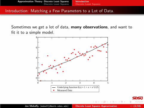
Introduction: Matching a Few Parameters to a Lot of Data.
Sometimes we get a lot of data, many observations, and want tofit it to a simple model.
0 1 2 3 4 5
0
2
4
6
8
Underlying function f(x) = 1 + x + x^2/25Measured Data
Joe Mahaffy, 〈[email protected]〉 Discrete Least Squares Approximation — (3/33)
Approximation Theory: Discrete Least SquaresDiscrete Least Squares
IntroductionDiscrete Least Squares
Introduction: Matching a Few Parameters to a Lot of Data.
Sometimes we get a lot of data, many observations, and want tofit it to a simple model.
0 1 2 3 4 5
0
2
4
6
8
Underlying function f(x) = 1 + x + x^2/25Measured DataAverageLinear Best FitQuadratic Best Fit
PDF-link: code.
Joe Mahaffy, 〈[email protected]〉 Discrete Least Squares Approximation — (3/33)

Approximation Theory: Discrete Least SquaresDiscrete Least Squares
IntroductionDiscrete Least Squares
Why a Low Dimensional Model?
Low dimensional models (e.g. low degree polynomials) are easy towork with, and are quite well behaved (high degree polynomialscan be quite oscillatory.)
All measurements are noisy, to some degree. Often, we want touse a large number of measurements in order to “average out”random noise.
Approximation Theory looks at two problems:
[1] Given a data set, find the best fit for a model (i.e. in a classof functions, find the one that best represents the data.)
[2] Find a simpler model approximating a given function.
Joe Mahaffy, 〈[email protected]〉 Discrete Least Squares Approximation — (4/33)

Approximation Theory: Discrete Least SquaresDiscrete Least Squares
IntroductionDiscrete Least Squares
Interpolation: A Bad Idea?
We can probably agree that trying to interpolate this data set:
0 1 2 3 4 5
0
2
4
6
8
Measured Data
with a 50th degree polynomial is not the best idea in the world...Even fitting a cubic spline to this data gives wild oscillations![I tried, and it was not pretty!]
Joe Mahaffy, 〈[email protected]〉 Discrete Least Squares Approximation — (5/33)

Approximation Theory: Discrete Least SquaresDiscrete Least Squares
IntroductionDiscrete Least Squares
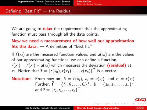
Defining “Best Fit” — the Residual.
We are going to relax the requirement that the approximatingfunction must pass through all the data points.
Now we need a measurement of how well our approximationfits the data. — A definition of “best fit.”
Joe Mahaffy, 〈[email protected]〉 Discrete Least Squares Approximation — (6/33)
Approximation Theory: Discrete Least SquaresDiscrete Least Squares
IntroductionDiscrete Least Squares
Defining “Best Fit” — the Residual.
We are going to relax the requirement that the approximatingfunction must pass through all the data points.
Now we need a measurement of how well our approximationfits the data. — A definition of “best fit.”
If f (xi ) are the measured function values, and a(xi ) are the valuesof our approximating functions, we can define a function,r(xi ) = f (xi ) − a(xi ) which measures the deviation (residual) atxi . Notice that r = {r(x0), r(x1), . . . , r(xn)}
T is a vector.
Notation: From now on, fi = f (xi ), ai = a(xi ), and ri = r(xi ).Further, f = {f0, f1, . . . , fn}
T , a = {a0, a1, . . . , an}T ,
and r = {r0, r1, . . . , rn}T .
Joe Mahaffy, 〈[email protected]〉 Discrete Least Squares Approximation — (6/33)
Approximation Theory: Discrete Least SquaresDiscrete Least Squares
IntroductionDiscrete Least Squares
What is the Size of the Residual?
There are many possible choices, e.g.
• The abs-sum of the deviations:
E1 =
n∑
i=0
|ri | ⇔ E1 = ‖r‖1
• The sum-of-the-squares of the deviations:
E2 =
√√√√
n∑
i=0
|ri |2 ⇔ E2 = ‖r‖2
• The largest of the deviations:
E∞ = max0≤i≤n
|ri | ⇔ E∞ = ‖r‖∞
In most cases, the sum-of-the-squares version is the easiest to workwith. (From now on we will focus on this choice...)
Joe Mahaffy, 〈[email protected]〉 Discrete Least Squares Approximation — (7/33)
Approximation Theory: Discrete Least SquaresDiscrete Least Squares
IntroductionDiscrete Least Squares
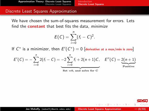
Discrete Least Squares Approximation
We have chosen the sum-of-squares measurement for errors. Letsfind the constant that best fits the data, minimize
E (C ) =n∑
i=0
(fi − C )2.
If C ∗ is a minimizer, then E ′(C ∗) = 0 [derivative at a max/min is zero]
Joe Mahaffy, 〈[email protected]〉 Discrete Least Squares Approximation — (8/33)
Approximation Theory: Discrete Least SquaresDiscrete Least Squares
IntroductionDiscrete Least Squares
Discrete Least Squares Approximation
We have chosen the sum-of-squares measurement for errors. Letsfind the constant that best fits the data, minimize
E (C ) =n∑
i=0
(fi − C )2.
If C ∗ is a minimizer, then E ′(C ∗) = 0 [derivative at a max/min is zero]
E ′(C ) = −
n∑
i=0
2(fi − C ) = −2
n∑
i=0
fi + 2(n + 1)C ,
︸ ︷︷ ︸
Set =0, and solve for C
E ′′(C ) = 2(n + 1)︸ ︷︷ ︸
Positive
Joe Mahaffy, 〈[email protected]〉 Discrete Least Squares Approximation — (8/33)
Approximation Theory: Discrete Least SquaresDiscrete Least Squares
IntroductionDiscrete Least Squares
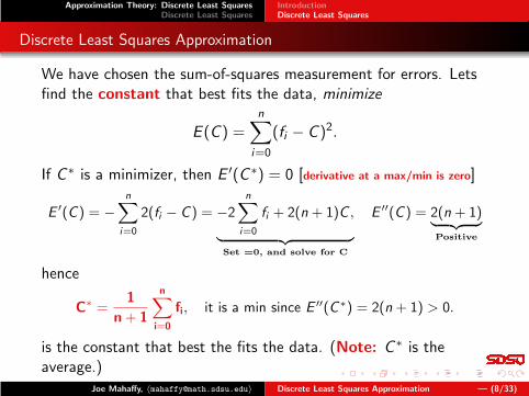
Discrete Least Squares Approximation
We have chosen the sum-of-squares measurement for errors. Letsfind the constant that best fits the data, minimize
E (C ) =n∑
i=0
(fi − C )2.
If C ∗ is a minimizer, then E ′(C ∗) = 0 [derivative at a max/min is zero]
E ′(C ) = −
n∑
i=0
2(fi − C ) = −2
n∑
i=0
fi + 2(n + 1)C ,
︸ ︷︷ ︸
Set =0, and solve for C
E ′′(C ) = 2(n + 1)︸ ︷︷ ︸
Positive
hence
C∗ =1
n + 1
n∑
i=0
fi, it is a min since E ′′(C∗) = 2(n + 1) > 0.
is the constant that best the fits the data. (Note: C ∗ is theaverage.)
Joe Mahaffy, 〈[email protected]〉 Discrete Least Squares Approximation — (8/33)
Approximation Theory: Discrete Least SquaresDiscrete Least Squares
IntroductionDiscrete Least Squares
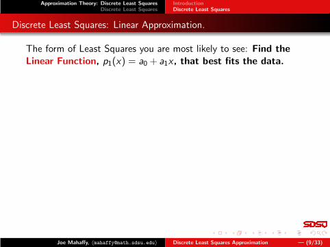
Discrete Least Squares: Linear Approximation.
The form of Least Squares you are most likely to see: Find theLinear Function, p1(x) = a0 + a1x, that best fits the data.
Joe Mahaffy, 〈[email protected]〉 Discrete Least Squares Approximation — (9/33)

Approximation Theory: Discrete Least SquaresDiscrete Least Squares
IntroductionDiscrete Least Squares
Discrete Least Squares: Linear Approximation.
The form of Least Squares you are most likely to see: Find theLinear Function, p1(x) = a0 + a1x, that best fits the data. Theerror E (a0, a1) we need to minimize is:
E (a0, a1) =
n∑
i=0
[(a0 + a1xi ) − fi ]2 .
The first partial derivatives with respect to a0 and a1 better bezero at the minimum:
∂
∂a0E (a0, a1) = 2
n∑
i=0
[(a0 + a1xi ) − fi ] = 0
∂
∂a1E (a0, a1) = 2
n∑
i=0
xi [(a0 + a1xi ) − fi ] = 0.
We “massage” these expressions to get the Normal Equations...
Joe Mahaffy, 〈[email protected]〉 Discrete Least Squares Approximation — (9/33)

Approximation Theory: Discrete Least SquaresDiscrete Least Squares
IntroductionDiscrete Least Squares
Linear Approximation: The Normal Equations p1(x)
n∑
i=0
[(a0 + a1xi ) − fi ] = 0
n∑
i=0
xi [(a0 + a1xi ) − fi ] = 0.
Joe Mahaffy, 〈[email protected]〉 Discrete Least Squares Approximation — (10/33)

Approximation Theory: Discrete Least SquaresDiscrete Least Squares
IntroductionDiscrete Least Squares
Linear Approximation: The Normal Equations p1(x)
n∑
i=0
a0 +n∑
i=0
a1xi −n∑
i=0
fi = 0
n∑
i=0
xia0 +n∑
i=0
xia1xi −n∑
i=0
xi fi = 0.
Joe Mahaffy, 〈[email protected]〉 Discrete Least Squares Approximation — (10/33)

Approximation Theory: Discrete Least SquaresDiscrete Least Squares
IntroductionDiscrete Least Squares
Linear Approximation: The Normal Equations p1(x)
a0(n + 1) + a1
n∑
i=0
xi =n∑
i=0
fi
a0
n∑
i=0
xi + a1
n∑
i=0
x2i =
n∑
i=0
xi fi .
Since everything except a0 and a1 is known, this is a 2-by-2system of equations.
(n + 1)n∑
i=0
xi
n∑
i=0
xi
n∑
i=0
x2i
[a0
a1
]
=
n∑
i=0
fi
n∑
i=0
xi fi
.
Joe Mahaffy, 〈[email protected]〉 Discrete Least Squares Approximation — (10/33)
Approximation Theory: Discrete Least SquaresDiscrete Least Squares
IntroductionDiscrete Least Squares
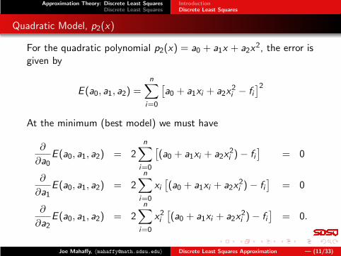
Quadratic Model, p2(x)
For the quadratic polynomial p2(x) = a0 + a1x + a2x2, the error is
given by
E (a0, a1, a2) =
n∑
i=0
[a0 + a1xi + a2x
2i − fi
]2
At the minimum (best model) we must have
∂
∂a0E (a0, a1, a2) = 2
n∑
i=0
[(a0 + a1xi + a2x
2i ) − fi
]= 0
∂
∂a1E (a0, a1, a2) = 2
n∑
i=0
xi
[(a0 + a1xi + a2x
2i ) − fi
]= 0
∂
∂a2E (a0, a1, a2) = 2
n∑
i=0
x2i
[(a0 + a1xi + a2x
2i ) − fi
]= 0.
Joe Mahaffy, 〈[email protected]〉 Discrete Least Squares Approximation — (11/33)

Approximation Theory: Discrete Least SquaresDiscrete Least Squares
IntroductionDiscrete Least Squares
Quadratic Model: The Normal Equations p2(x)
Similarly for the quadratic polynomial p2(x) = a0 + a1x + a2x2,
the normal equations are:
a0(n + 1) + a1
n∑
i=0
xi + a2
n∑
i=0
x2i =
n∑
i=0
fi
a0
n∑
i=0
xi + a1
n∑
i=0
x2i + a2
n∑
i=0
x3i =
n∑
i=0
xi fi .
a0
n∑
i=0
x2i + a1
n∑
i=0
x3i + a2
n∑
i=0
x4i =
n∑
i=0
x2i fi .
Note: Even though the model is quadratic, the resulting (normal)equations are linear. — The model is linear in its parame-ters, a0, a1, and a2.
Joe Mahaffy, 〈[email protected]〉 Discrete Least Squares Approximation — (12/33)

Approximation Theory: Discrete Least SquaresDiscrete Least Squares
IntroductionDiscrete Least Squares
The Normal Equations — As Matrix Equations.
We have:
a0(n + 1) + a1
n∑
i=0
xi + a2
n∑
i=0
x2i =
n∑
i=0
fi
a0
n∑
i=0
xi + a1
n∑
i=0
x2i + a2
n∑
i=0
x3i =
n∑
i=0
xi fi .
a0
n∑
i=0
x2i + a1
n∑
i=0
x3i + a2
n∑
i=0
x4i =
n∑
i=0
x2i fi .
Joe Mahaffy, 〈[email protected]〉 Discrete Least Squares Approximation — (13/33)

Approximation Theory: Discrete Least SquaresDiscrete Least Squares
IntroductionDiscrete Least Squares
The Normal Equations — As Matrix Equations.
We rewrite the Normal Equations as:
(n + 1)n∑
i=0
xi
n∑
i=0
x2i
n∑
i=0
xi
n∑
i=0
x2i
n∑
i=0
x3i
n∑
i=0
x2i
n∑
i=0
x3i
n∑
i=0
x4i
a0
a1
a2
=
n∑
i=0
fi
n∑
i=0
xi fi .
n∑
i=0
x2i fi .
.
It is not immediately obvious, but this expression can be written inthe form ATAa = ATf. Where the matrix A is very easy to writein terms of xi . [Jump Forward].
Joe Mahaffy, 〈[email protected]〉 Discrete Least Squares Approximation — (13/33)

Approximation Theory: Discrete Least SquaresDiscrete Least Squares
IntroductionDiscrete Least Squares
The Polynomial Equations in Matrix Form pm(x)
We can express the mth degree polynomial, pm(x), evaluated atthe points xi :
a0 + a1xi + a2x2i + · · · + amxm
i = fi , i = 0, . . . , n
as a product of an (n + 1)-by-(m + 1) matrix, A and the(m + 1)-by-1 vector a and the result is the (n + 1)-by-1 vector f,usually n ≫ m:
1 x0 x20 · · · xm
0
1 x1 x21 · · · xm
1
1 x2 x22 · · · xm
2
1 x3 x23 · · · xm
3...
......
......
1 xn x2n · · · xm
n
︸ ︷︷ ︸
A
a0
a1...
am
︸ ︷︷ ︸
a
=
f0f1f2f3...fn
︸ ︷︷ ︸
f
.
Joe Mahaffy, 〈[email protected]〉 Discrete Least Squares Approximation — (14/33)
Approximation Theory: Discrete Least SquaresDiscrete Least Squares
IntroductionDiscrete Least Squares
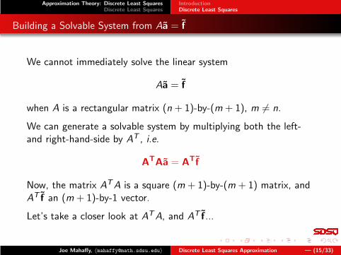
Building a Solvable System from Aa = f
We cannot immediately solve the linear system
Aa = f
when A is a rectangular matrix (n + 1)-by-(m + 1), m 6= n.
We can generate a solvable system by multiplying both the left-and right-hand-side by AT , i.e.
ATAa = ATf
Now, the matrix ATA is a square (m + 1)-by-(m + 1) matrix, andAT f an (m + 1)-by-1 vector.
Let’s take a closer look at ATA, and AT f...
Joe Mahaffy, 〈[email protected]〉 Discrete Least Squares Approximation — (15/33)

Approximation Theory: Discrete Least SquaresDiscrete Least Squares
IntroductionDiscrete Least Squares
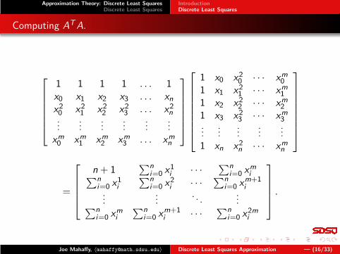
Computing ATA.
1 1 1 1 . . . 1x0 x1 x2 x3 . . . xn
x20 x2
1 x22 x2
3 . . . x2n
......
......
......
xm0 xm
1 xm2 xm
3 . . . xmn
1 x0 x20 · · · xm
0
1 x1 x21 · · · xm
1
1 x2 x22 · · · xm
2
1 x3 x23 · · · xm
3...
......
......
1 xn x2n · · · xm
n
=
n + 1 ◦ ◦ ◦◦ ◦ ◦ ◦◦ ◦ ◦ ◦◦ ◦ ◦ ◦
Joe Mahaffy, 〈[email protected]〉 Discrete Least Squares Approximation — (16/33)

Approximation Theory: Discrete Least SquaresDiscrete Least Squares
IntroductionDiscrete Least Squares
Computing ATA.
1 1 1 1 . . . 1x0 x1 x2 x3 . . . xn
x20 x2
1 x22 x2
3 . . . x2n
......
......
......
xm0 xm
1 xm2 xm
3 . . . xmn
1 x0 x20 · · · xm
0
1 x1 x21 · · · xm
1
1 x2 x22 · · · xm
2
1 x3 x23 · · · xm
3...
......
......
1 xn x2n · · · xm
n
=
n + 1 ◦ ◦∑n
i=0 xmi
◦ ◦ ◦ ◦◦ ◦ ◦ ◦◦ ◦ ◦ ◦
Joe Mahaffy, 〈[email protected]〉 Discrete Least Squares Approximation — (16/33)

Approximation Theory: Discrete Least SquaresDiscrete Least Squares
IntroductionDiscrete Least Squares
Computing ATA.
1 1 1 1 . . . 1x0 x1 x2 x3 . . . xn
x20 x2
1 x22 x2
3 . . . x2n
......
......
......
xm0 xm
1 xm2 xm
3 . . . xmn
1 x0 x20 · · · xm
0
1 x1 x21 · · · xm
1
1 x2 x22 · · · xm
2
1 x3 x23 · · · xm
3...
......
......
1 xn x2n · · · xm
n
=
n + 1 ◦ ◦∑n
i=0 xmi
◦ ◦ ◦ ◦◦ ◦ ◦ ◦
∑ni=0 xm
i ◦ ◦ ◦
Joe Mahaffy, 〈[email protected]〉 Discrete Least Squares Approximation — (16/33)
Approximation Theory: Discrete Least SquaresDiscrete Least Squares
IntroductionDiscrete Least Squares
Computing ATA.
1 1 1 1 . . . 1x0 x1 x2 x3 . . . xn
x20 x2
1 x22 x2
3 . . . x2n
......
......
......
xm0 xm
1 xm2 xm
3 . . . xmn
1 x0 x20 · · · xm
0
1 x1 x21 · · · xm
1
1 x2 x22 · · · xm
2
1 x3 x23 · · · xm
3...
......
......
1 xn x2n · · · xm
n
=
n + 1 ◦ ◦∑n
i=0 xmi
◦ ◦ ◦ ◦◦ ◦ ◦ ◦
∑ni=0 xm
i ◦ ◦∑n
i=0 x2mi
Joe Mahaffy, 〈[email protected]〉 Discrete Least Squares Approximation — (16/33)
Approximation Theory: Discrete Least SquaresDiscrete Least Squares
IntroductionDiscrete Least Squares
Computing ATA.
1 1 1 1 . . . 1x0 x1 x2 x3 . . . xn
x20 x2
1 x22 x2
3 . . . x2n
......
......
......
xm0 xm
1 xm2 xm
3 . . . xmn
1 x0 x20 · · · xm
0
1 x1 x21 · · · xm
1
1 x2 x22 · · · xm
2
1 x3 x23 · · · xm
3...
......
......
1 xn x2n · · · xm
n
=
n + 1∑n
i=0 x1i · · ·
∑ni=0 xm
i∑ni=0 x1
i
∑ni=0 x2
i · · ·∑n
i=0 xm+1i
......
. . ....
∑ni=0 xm
i
∑ni=0 xm+1
i · · ·∑n
i=0 x2mi
.
Joe Mahaffy, 〈[email protected]〉 Discrete Least Squares Approximation — (16/33)

Approximation Theory: Discrete Least SquaresDiscrete Least Squares
IntroductionDiscrete Least Squares
Computing AT f .
1 1 1 1 . . . 1x0 x1 x2 x3 . . . xn
x20 x2
1 x22 x2
3 . . . x2n
......
......
......
xm0 xm
1 xm2 xm
3 . . . xmn
f0f1f2f3...fn
=
∑ni=0 fi
∑ni=0 xi fi
∑ni=0 x2
i fi...
∑ni=0 xm
i fi .
We have recovered the Normal Equations...
[Jump Back].
Joe Mahaffy, 〈[email protected]〉 Discrete Least Squares Approximation — (17/33)

Approximation Theory: Discrete Least SquaresDiscrete Least Squares
A Simple, Powerful Approach
Discrete Least Squares: A Simple, Powerful Method.
Given the data set (x, f), where x = {x0, x1, . . . , xn}T and
f = {f0, f1, . . . , fn}T , we can quickly find the best polynomial fit for
any specified polynomial degree!
Notation: Let xj be the vector {x j0, x
j1, . . . , x
jn}
T .
E.g. to compute the best fitting polynomial of degree 3,p3(x) = a0 + a1x + a2x
2 + a3x3, define:
A =
| | | || | | |
1 x x2 x3
| | | || | | |
, and compute a = (ATA)−1(AT f).
Joe Mahaffy, 〈[email protected]〉 Discrete Least Squares Approximation — (18/33)

Approximation Theory: Discrete Least SquaresDiscrete Least Squares
A Simple, Powerful Approach
Discrete Least Squares: Matlab Example.
I used this code to generate the data for the plots on slide 2.
x = (0:0.1:5)’; % The x-vector
f = 1+x+x.∧2/25; % The underlying function
n = randn(size(x)); % Random perturbations
fn = f+n; % Add randomness
A = [x ones(size(x))]; % Build A for linear fit
%a = (A’*A)\(A’*f); % Solve
a = A\f; % Better, Equivalent, Solve
p1 = polyval(a,x); % Evaluate
A = [x.∧2 x ones(size(x))]; % A for quadratic fit
%a = (A’*A)\(A’*f); % Solve
a = A\f; % Better, Equivalent, Solve
p2 = polyval(a,x); % Evaluate
Joe Mahaffy, 〈[email protected]〉 Discrete Least Squares Approximation — (19/33)
Approximation Theory: Discrete Least SquaresDiscrete Least Squares
A Simple, Powerful Approach
But... I do not want to fit a polynomial!!!
Fitting an exponential model g(x) = becx to the given data d, isquite straight-forward.
Joe Mahaffy, 〈[email protected]〉 Discrete Least Squares Approximation — (20/33)

Approximation Theory: Discrete Least SquaresDiscrete Least Squares
A Simple, Powerful Approach
But... I do not want to fit a polynomial!!!
Fitting an exponential model g(x) = becx to the given data d, isquite straight-forward.
First, re-cast the problem as a set of linear equations. We have:
becxi = di , i = 0, . . . , n
compute the natural logarithm on both sides:
ln b︸︷︷︸
a0
+ c︸︷︷︸
a1
xi = ln di︸︷︷︸
fi
.
Now, we can apply a polynomial least squares fit to the problem,and once we have (a0, a1), b = ea0 and c = a1.
Note: This does not give the least squares fit to the original prob-lem!!! (It gives us a pretty good estimate.)
Joe Mahaffy, 〈[email protected]〉 Discrete Least Squares Approximation — (20/33)

Approximation Theory: Discrete Least SquaresDiscrete Least Squares
A Simple, Powerful Approach
But... That is not a True Least Squares Fit!
Note: Fitting the modified problem does not give the leastsquares fit to the original problem!!!
In order to find the true least squares fit we need to know how tofind roots and/or minima/maxima of non-linear systems ofequations.
Feel free to sneak a peek at Burden-Faires chapter 10.Unfortunately we do not have the time to talk about this here...
What we need: Math 693a — Numerical OptimizationTechniques.
Some of this stuff may show up in a different context in: Math 562— Mathematical Methods of Operations Research.
Joe Mahaffy, 〈[email protected]〉 Discrete Least Squares Approximation — (21/33)
Discrete Least Squares Application: Cricket Thermometer
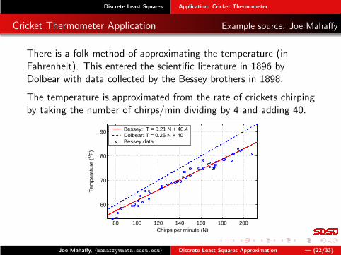
Cricket Thermometer Application Example source: Joe Mahaffy
There is a folk method of approximating the temperature (inFahrenheit). This entered the scientific literature in 1896 byDolbear with data collected by the Bessey brothers in 1898.
The temperature is approximated from the rate of crickets chirpingby taking the number of chirps/min dividing by 4 and adding 40.
80 100 120 140 160 180 200
60
70
80
90
Chirps per minute (N)
Tem
pera
ture
( o F
)
Bessey: T = 0.21 N + 40.4Dolbear: T = 0.25 N + 40Bessey data
Joe Mahaffy, 〈[email protected]〉 Discrete Least Squares Approximation — (22/33)

Discrete Least Squares Application: Cricket Thermometer
Cricket Data Analysis
C. A. Bessey and E. A. Bessey collected data on eight differentcrickets that they observed in Lincoln, Nebraska during August andSeptember, 1897. The number of chirps/min was N and thetemperature was T .
Create matrices
A1 =
1 N1
1 N2...
...
A2 =
1 N1 N21
1 N2 N22
......
...
A3 =
1 N1 N21 N3
1
1 N2 N22 N3
2...
......
...
A4 =
1 N1 N21 N3
1 N41
1 N2 N22 N3
2 N42
......
......
Joe Mahaffy, 〈[email protected]〉 Discrete Least Squares Approximation — (23/33)

Discrete Least Squares Application: Cricket Thermometer
Cricket Linear Model
If you compute the matrix which you never should!
AT1 A1 =
(52 7447
7447 1133259
)
,
it has eigenvalues
λ1 = 3.0633 and λ2 = 1, 133, 308,
which gives the condition number
cond(AT1 A1) = 3.6996 × 10⁵.
Whereascond(A1) = 608.2462.
In MatlabA1\T
gives the parameters for best linear model
T1(N) = 0.2155N + 39.7441.
Joe Mahaffy, 〈[email protected]〉 Discrete Least Squares Approximation — (24/33)

Discrete Least Squares Application: Cricket Thermometer
Polynomial Fits to the Data: Linear
Linear Fit
Joe Mahaffy, 〈[email protected]〉 Discrete Least Squares Approximation — (25/33)

Discrete Least Squares Application: Cricket Thermometer
Cricket Quadratic Model
Similarly, the matrix
AT2 A2 =
52 7447 11332597447 1133259 1.8113 × 10⁸
1133259 1.8113 × 10⁸ 3.0084 × 10¹⁰
,
has eigenvalues
λ1 = 0.1957, λ2 = 42, 706, λ3 = 3.00853 × 10¹⁰
which gives the condition number
cond(AT2 A2) = 1.5371 × 10¹¹.
Whereas,cond(A2) = 3.9206 × 10⁵,
andA2\T,
gives the parameters for best quadratic model
T2(N) = −0.00064076N2 + 0.39625N + 27.8489.
Joe Mahaffy, 〈[email protected]〉 Discrete Least Squares Approximation — (26/33)

Discrete Least Squares Application: Cricket Thermometer
Polynomial Fits to the Data: Quadratic
Quadratic Fit
Joe Mahaffy, 〈[email protected]〉 Discrete Least Squares Approximation — (27/33)

Discrete Least Squares Application: Cricket Thermometer
Cricket Cubic and Quartic Models
The condition numbers for the cubic and quartic rapidly get larger with
cond(AT3 A3) = 6.3648 × 10¹⁶ and cond(AT
4 A4) = 1.1218 × 10²³
These last two condition numbers suggest that any coefficients obtainedare highly suspect.
However, if done right, we are “only” subject to the conditon numbers
cond(A3) = 2.522 × 10⁸, cond(A4) = 1.738 × 10¹¹.
The best cubic and quartic models are given by
T3(N) = 0.0000018977N3 − 0.001445N2 + 0.50540N + 23.138
T4(N) = −0.00000001765N4 + 0.00001190N3 − 0.003504N2
= +0.6876N + 17.314
Joe Mahaffy, 〈[email protected]〉 Discrete Least Squares Approximation — (28/33)

Discrete Least Squares Application: Cricket Thermometer
Polynomial Fits to the Data: Cubic
Cubic Fit
Joe Mahaffy, 〈[email protected]〉 Discrete Least Squares Approximation — (29/33)

Discrete Least Squares Application: Cricket Thermometer
Polynomial Fits to the Data: Quartic
Quartic Fit
Joe Mahaffy, 〈[email protected]〉 Discrete Least Squares Approximation — (30/33)

Discrete Least Squares Application: Cricket Thermometer
Best Cricket Model
So how does one select the best model?
Visually, one can see that the linear model does a very good job,and one only obtains a slight improvement with a quadratic. Is itworth the added complication for the slight improvement.
It is clear that the sum of square errors (SSE) will improve as thenumber of parameters increase.
From statistics, it is hotly debated how much penalty one shouldpay for adding parameters.
Joe Mahaffy, 〈[email protected]〉 Discrete Least Squares Approximation — (31/33)

Discrete Least Squares Application: Cricket Thermometer
Best Cricket Model - Analysis
Bayesian Information Criterion
Let n be the number of data points, SSE be the sum of squareerrors, and let k be the number of parameters in the model.
BIC = n ln(SSE/n) + k ln(n).
Akaike Information Criterion
AIC = 2k + n(ln(2πSSE/n) + 1).
Joe Mahaffy, 〈[email protected]〉 Discrete Least Squares Approximation — (32/33)

Discrete Least Squares Application: Cricket Thermometer
Best Cricket Model - Analysis Continued
The table below shows the by the Akaike information criterion thatwe should take a quadratic model, while using a BayesianInformation Criterion we should use a cubic model.
Linear Quadratic Cubic Quartic
SSE 108.8 79.08 78.74 78.70
BIC 46.3 33.65 33.43 37.35
AIC 189.97 175.37 177.14 179.12
Returning to the original statement, we do fairly well by using thefolk formula, despite the rest of this analysis!
Joe Mahaffy, 〈[email protected]〉 Discrete Least Squares Approximation — (33/33)