Numerical Algorithms

•Matrix multiplication•Numerical solution of Linear System of Equations

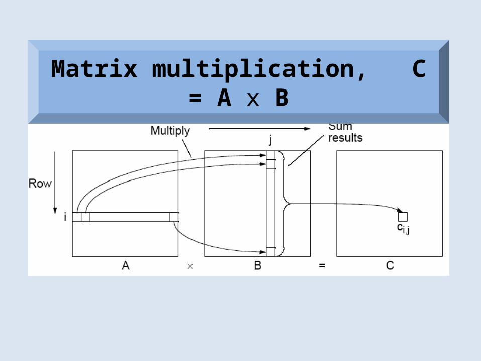
Matrix multiplication, C = A x B

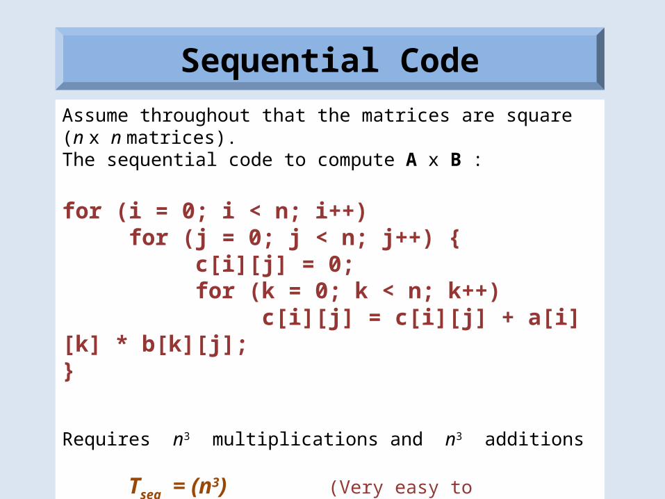
Assume throughout that the matrices are square (n x n matrices).The sequential code to compute A x B :

for (i = 0; i < n; i++)for (j = 0; j < n; j++) {

c[i][j] = 0;for (k = 0; k < n; k++)

c[i][j] = c[i][j] + a[i][k] * b[k][j];}

Requires n3 multiplications and n3 additions

Tseq = (n3) (Very easy to parallelize!)

Sequential Code

• One PE to compute each element of C - n2 processors would be needed.

• Each PE holds one row of elements of A and one column of elements of B.

Direct Implementation (P=n2)

P = n2 Tpar = O(n)

P = n3 Tpar = O(log n)

• n processors collaborate in computing each element of C - n3 processors are needed.

• Each PE holds one element of A and one element of B.

Performance Improvement (P=n3)

• P = n Tpar = O(n2) Each instance of inner loop is independent and can be done by a separate processor.Cost optimal since O(n3) = n * O(n2)

• P = n2 Tpar = O(n) One element of C (cij) is assigned to each processor.Cost optimal since O(n3) = n2 x O(n)

• P = n3 Tpar = O(log n) n processors compute one element of C (cij) in parallel (O(log n))Not cost optimal since O(n3) < n3 * O(log n)

O(log n) lower bound for parallel matrix multiplication.

Parallel Matrix Multiplication - Summary

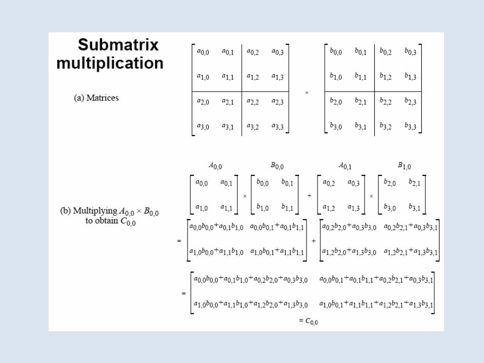
Block Matrix Multiplication

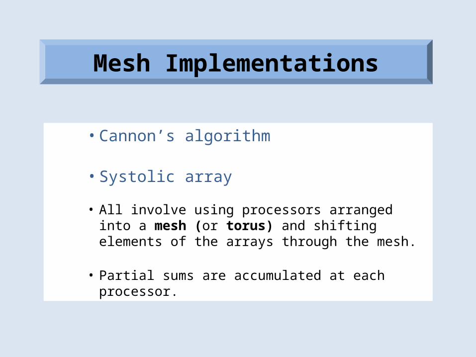
• Cannon’s algorithm

• Systolic array

• All involve using processors arranged into a mesh (or torus) and shifting elements of the arrays through the mesh.

• Partial sums are accumulated at each processor.

Mesh Implementations

Elements Need to Be Aligned

A00

B00

A01

B01

A02

B02

A03

B03

A10

B10

A11

B11

A12

B12

A13

B13

A20

B20

A21

B21

A22

B22

A23

B23

A30

B30

A31

B31

A32

B32

A33

B33

Each trianglerepresents a matrix element (or a block)

Only same-colortriangles shouldbe multiplied

Alignment of elements of A and B

Before After

A00

B00

A01

B01

A02

B02

A03

B03

A10

B10

A11

B11

A12

B12

A13

B13

A20

B20

A21

B21

A22

B22

A23

B23

A30

B30

A31

B31

A32

B32

A33

B33

Ai* (ith row) cyclesleft i positions

B*j (jth column) cycles up j positions

Alignment

Shift, multiply, addConsider Process P1,2

B02

A10A11 A12

B12

A13

B22

B32 Step 1

B12

A11A12 A13

B22

A10

B32

B02 Step 2

Shift, multiply, addConsider Process P1,2

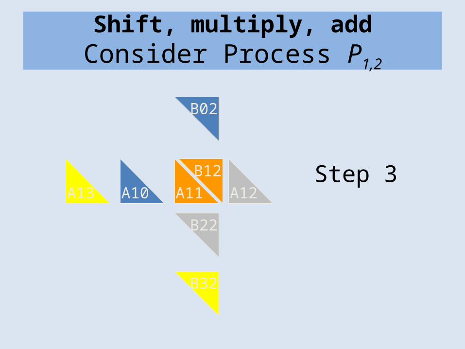
B22

A12A13 A10

B32

A11

B02

B12 Step 3

Shift, multiply, addConsider Process P1,2

B32

A13A10 A11

B02

A12

B12

B22 Step 4

Shift, multiply, addConsider Process P1,2

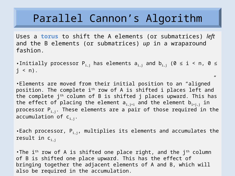
Uses a torus to shift the A elements (or submatrices) left and the B elements (or submatrices) up in a wraparound fashion.

•Initially processor Pi,j has elements ai,j and bi,j (0 ≤ i < n, 0 ≤ j < n).

•Elements are moved from their initial position to an “aligned” position. The complete i th row of A is shifted i places left and the complete jth column of B is shifted j places upward. This has the effect of placing the element ai,j+i and the element bi+j,j in processor Pi,j. These elements are a pair of those required in the accumulation of c i,j.

•Each processor, Pi,j, multiplies its elements and accumulates the result in c i,j

•The ith row of A is shifted one place right, and the jth column of B is shifted one place upward. This has the effect of bringing together the adjacent elements of A and B, which will also be required in the accumulation.

•Each PE (Pi,j) multiplies the elements brought to it and adds the result to the accumulating sum.

•The last two steps are repeated until the final result is obtained (n-1 shifts)

Parallel Cannon’s Algorithm

Time Complexity

• P = n2 A, B: n x n matrices with n2 elements each

One element of C (cij) is assigned to each processor.Alignment step takes O(n) steps.Therefore,

Tpar = O(n)

Cost optimal since O(n3) = n2 * O(n)Also, highly scalable!

Systolic Array

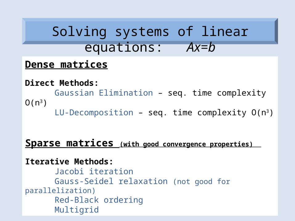
Dense matrices

Direct Methods:Gaussian Elimination – seq. time complexity O(n3)LU-Decomposition – seq. time complexity O(n3)

Sparse matrices (with good convergence properties)

Iterative Methods:Jacobi iterationGauss-Seidel relaxation (not good for parallelization)Red-Black orderingMultigrid

Solving systems of linear equations: Ax=b

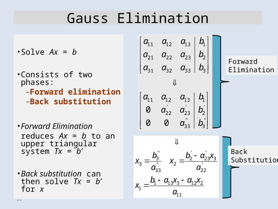
• Solve Ax = b

• Consists of two phases:–Forward elimination–Back substitution

• Forward Eliminationreduces Ax = b to an upper triangular system Tx = b’

• Back substitution can then solve Tx = b’ for x

11

21231311

22

32322

33

33

333

22322

1131211

3333231

2232221

1131211

00

0

a

xaxabx

a

xabx

a

bx

ba

baa

baaa

baaa

baaa

baaa

'

''

''

''

''''

'''

ForwardElimination

BackSubstitution

Gauss Elimination

22

Gauss Elimination

• Solve Ax = b

• Consists of two phases:–Forward elimination–Back substitution

• Forward Eliminationreduces Ax = b to an upper triangular system Tx = b’

• Back substitution can then solve Tx = b’ for x

''3

''33

'2

'23

'22

1131211

3333231

2232221

1131211

00

0

ba

baa

baaa

baaa

baaa

baaa

ForwardElimination

BackSubstitution

11

21231311

'22

3'23

'2

2''33

''3

3

a

xaxabx

a

xabx

a

bx

23

Gaussian EliminationForward Elimination

x1 - x2 + x3 = 6 3x1 + 4x2 + 2x3 = 9 2x1 + x2 + x3 = 7

x1 - x2 + x3 = 6 0 +7x2 - x3 = -9 0 + 3x2 - x3 = -5

x1 - x2 + x3 = 6 0 7x2 - x3 = -9 0 0 -(4/7)x3=-(8/7)

-(3/1)

Solve using BACK SUBSTITUTION: x3 = 2 x2=-1 x1 =3

-(2/1) -(3/7)

0

0

0

0

0

0

0

0

0

0

0

0

0

0

0

0

0

0

0

0

0

0

0

0

0

0

0

0

0

0

0

0

0

0

0 0

24

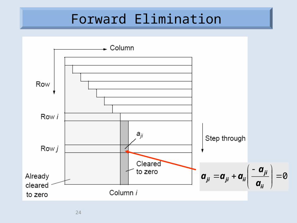
Forward Elimination

0

ii

jiiijiji a

aaaa

25

4x0 +6x1 +2x2 – 2x3 = 8

2x0 +5x2 – 2x3 = 4

–4x0 – 3x1 – 5x2 +4x3 = 1

8x0 +18x1 – 2x2 +3x3 = 40

-(2/4)

MULTIPLIERS

-(-4/4)

-(8/4)

Gaussian Elimination

26

4x0 +6x1 +2x2 – 2x3 = 8

+4x2 – 1x3 = 0

+3x1 – 3x2 +2x3 = 9

+6x1 – 6x2 +7x3 = 24

– 3x1

-(3/-3)

MULTIPLIERS

-(6/-3)

Gaussian Elimination

27

4x0 +6x1 +2x2 – 2x3 = 8

+4x2 – 1x3 = 0

1x2 +1x3 = 9

2x2 +5x3 = 24

– 3x1

??

MULTIPLIER

Gaussian Elimination

28

4x0 +6x1 +2x2 – 2x3 = 8

+4x2 – 1x3 = 0

1x2 +1x3 = 9

3x3 = 6

– 3x1

Gaussian Elimination

29

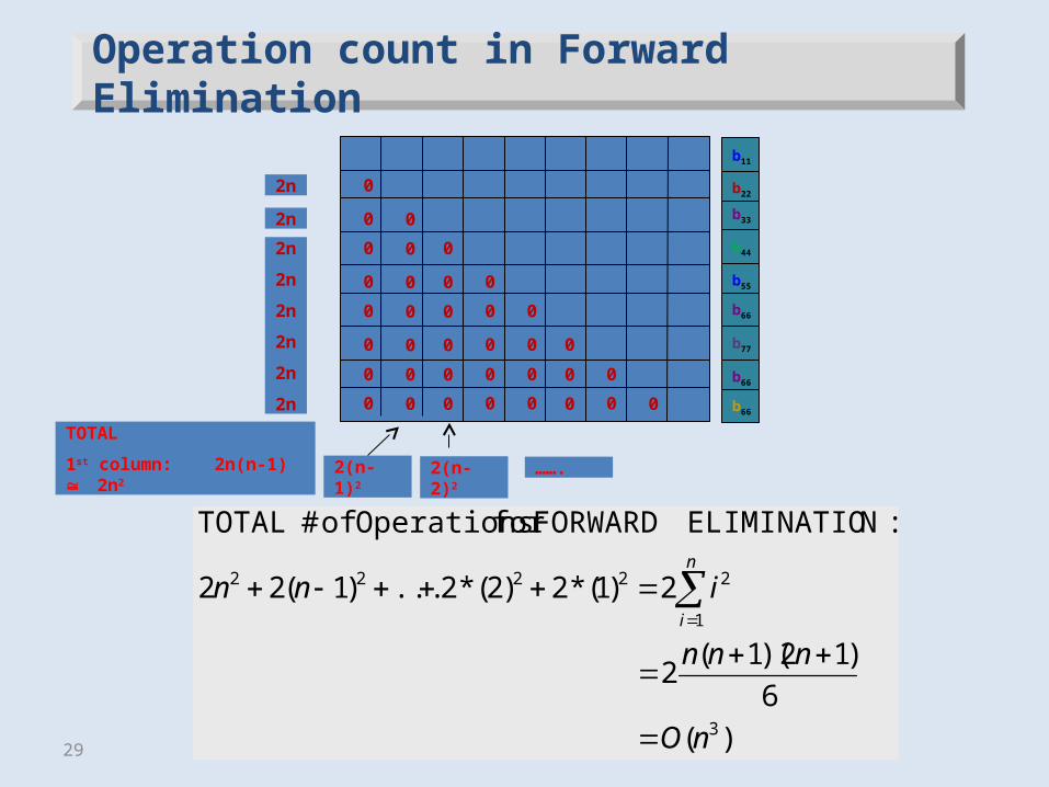
Gaussian EliminationOperation count in Forward Elimination

0

0

0

0

0

0

0

0

0

0

0

0

0

0

0

0

0

0

0

0

0

0

0

0

0

0

0

0

0

0

0

0

0

0

0 0

2n

2n

2n

2n

2n

2n

2n

2n

TOTAL

1st column: 2n(n-1) 2n2

)(

6

)12)(1(2

2)1(*2)2(*2...)1(22

:NELIMINATIO FORWARDfor Operations of # TOTAL

3

1

22222

nO

nnn

innn

i

2(n-1)2 2(n-2)2 …….

b11

b22

b33

b44

b55

b66

b77

b66

b66

30

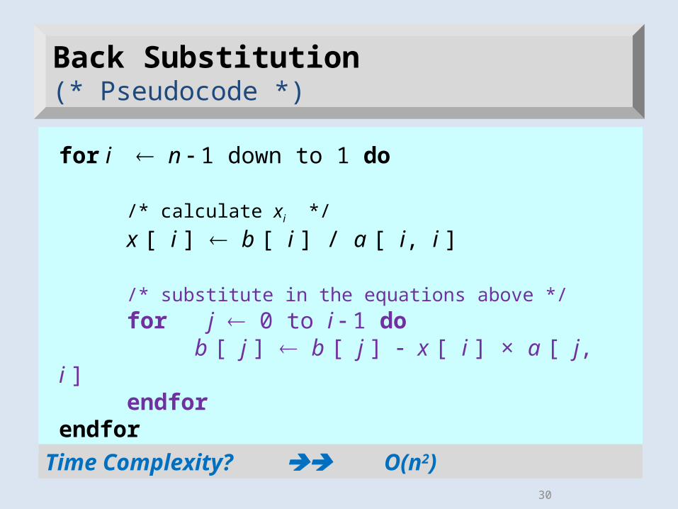
for i n 1 down to 1 do

/* calculate xi */

x [ i ] b [ i ] / a [ i, i ]

/* substitute in the equations above */for j 0 to i 1 do

b [ j ] b [ j ] x [ i ] × a [ j, i ]endfor

endfor

Back Substitution(* Pseudocode *)

Time Complexity? O(n2)

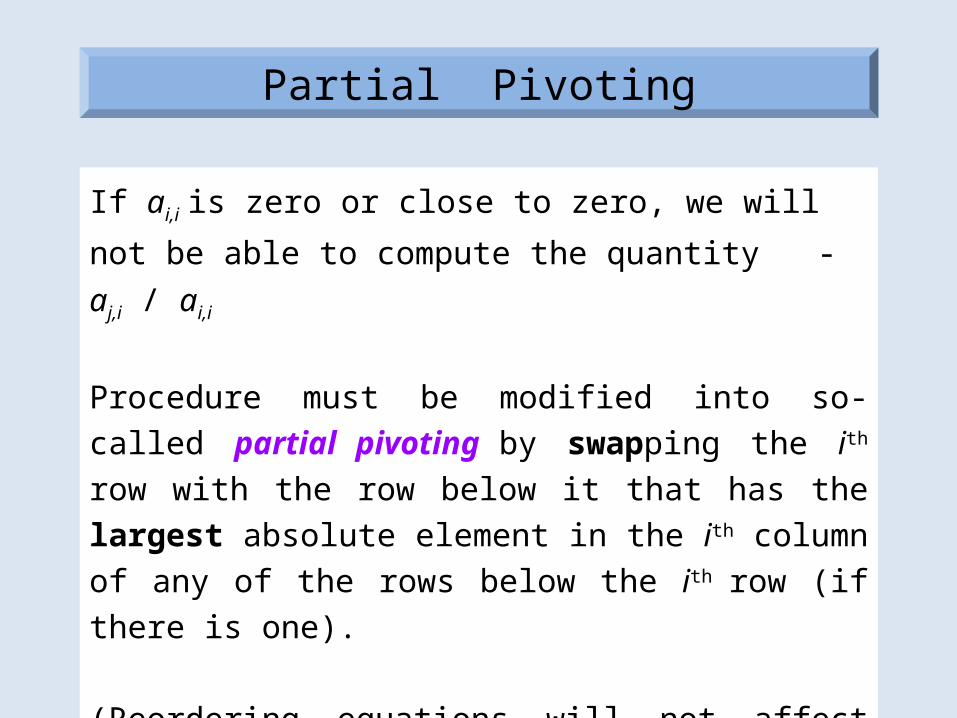
If ai,i is zero or close to zero, we will not be able to compute

the quantity -aj,i / ai,i

Procedure must be modified into so-called partial pivoting

by swapping the ith row with the row below it that has the

largest absolute element in the ith column of any of the rows

below the ith row (if there is one).

(Reordering equations will not affect the system.)

Partial Pivoting

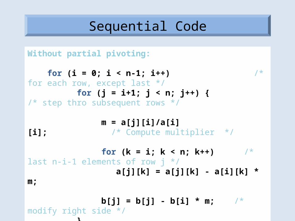
Without partial pivoting:

for (i = 0; i < n-1; i++) /* for each row, except last */ for (j = i+1; j < n; j++) { /* step thro subsequent rows */

m = a[j][i]/a[i][i]; /* Compute multiplier */

for (k = i; k < n; k++) /* last n-i-1 elements of row j */ a[j][k] = a[j][k] - a[i][k] * m;

b[j] = b[j] - b[i] * m; /* modify right side */ }

The time complexity: Tseq = O(n3)

Sequential Code

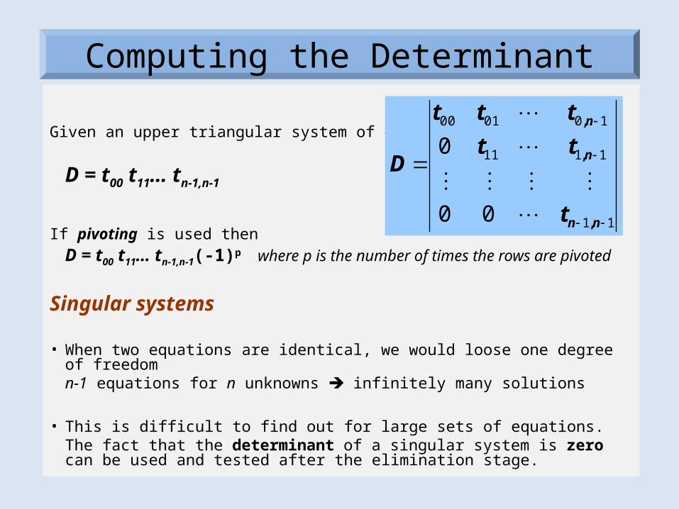
Given an upper triangular system of equations

D = t00 t11… tn-1,n-1

If pivoting is used then

D = t00 t11… tn-1,n-1(-1)p where p is the number of times the rows are pivoted

Singular systems

• When two equations are identical, we would loose one degree of freedom n-1 equations for n unknowns infinitely many solutions

• This is difficult to find out for large sets of equations. The fact that the determinant of a singular system is zero can be used and tested after the elimination stage.

11

1111

100100

00

0

nn

n

n

t

tt

ttt

D

,

,

,

Computing the Determinant

Parallel implementation

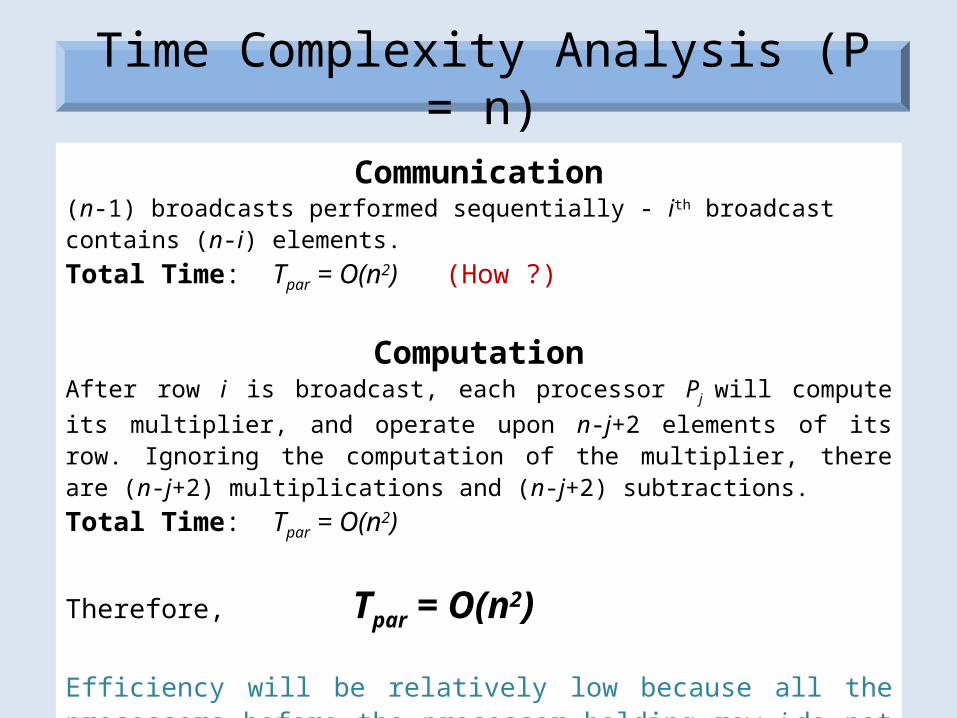
Communication(n-1) broadcasts performed sequentially - ith broadcast contains (n-i) elements.

Total Time: Tpar = O(n2) (How ?)

ComputationAfter row i is broadcast, each processor Pj will compute its multiplier, and operate

upon n-j+2 elements of its row. Ignoring the computation of the multiplier, there are (n-j+2) multiplications and (n-j+2) subtractions.

Total Time: Tpar = O(n2)

Therefore, Tpar = O(n2)

Efficiency will be relatively low because all the processors before the processor holding row i do not participate in the computation again.

Time Complexity Analysis (P = n)

Poor processor allocation! Processors do not participate in computation after their last row is processed.

Strip Partitioning

An alternative which equalizes the processor workload

Cyclic-Striped Partitioning

Jacobi Iterative Method (Sequential)

])([ )( )]([

xDAbDxxDAbDxbxDAD

a

a

a

D

aaa

aaa

aaa

AbAx

1

33

22

11

333231

232221

131211

00

00

00

33

1232

11313

322

1323

11212

211

1313

12121

1 a

xaxabx

a

xaxabx

a

xaxabx

kkk

kkk

kkk

1 11 1 12 13 1

2 22 2 21 23 2

3 33 3 31 32 3

1/ 0 0 0

0 1/ 0 * 0

0 0 1/ 0new old

x a b a a x

x a b a a x

x a b a a x

Choose an initial guess (i.e. all zeros) and Iterate until the equality is satisfied. No guarantee for convergence! Each iteration takes O(n2) time!

Iterative methods provide an alternative to the elimination methods.

• The Gauss-Seidel method is a commonly used iterative method.

• It is same as Jacobi technique except with one important difference:

A newly computed x value (say xk) is substituted in the subsequent equations (equations k+1, k+2, …, n) in the same iteration.

Example: Consider the 3x3 system below:

• First, choose initial guesses for the x’s.

• A simple way to obtain initial guesses is to assume that they are all zero.

• Compute new x1 using the previous iteration values.

• New x1 is substituted in the equations to calculate x2 and x3

• The process is repeated for x2, x3, …newold

newnewnew

oldnewnew

oldoldnew

XX

a

xaxabx

a

xaxabx

a

xaxabx

}{}{

33

23213133

22

32312122

11

31321211

Gauss-Seidel Method (Sequential)

Convergence Criterion for Gauss-Seidel Method

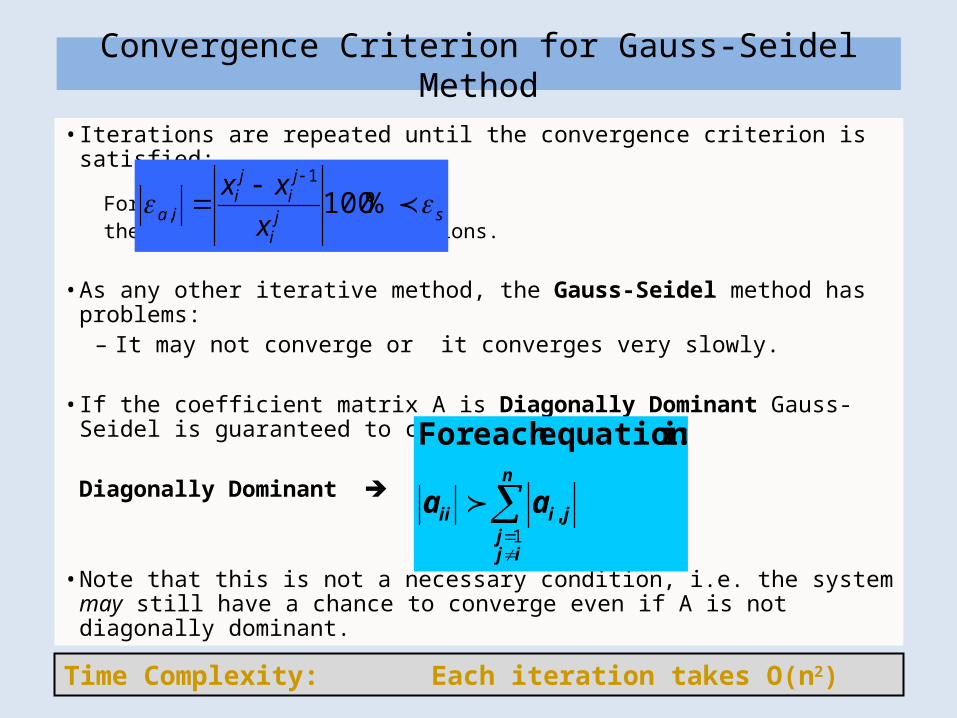
• Iterations are repeated until the convergence criterion is satisfied:

For all i, where j and j-1 are the current and previous iterations.

• As any other iterative method, the Gauss-Seidel method has problems:– It may not converge or it converges very slowly.

• If the coefficient matrix A is Diagonally Dominant Gauss-Seidel is guaranteed to converge.

Diagonally Dominant

• Note that this is not a necessary condition, i.e. the system may still have a chance to converge even if A is not diagonally dominant.

40

n

ijj

jiii aa1

,

:i equation eachFor

sji

ji

ji

ia x

xx %1001

,

Time Complexity: Each iteration takes O(n2)

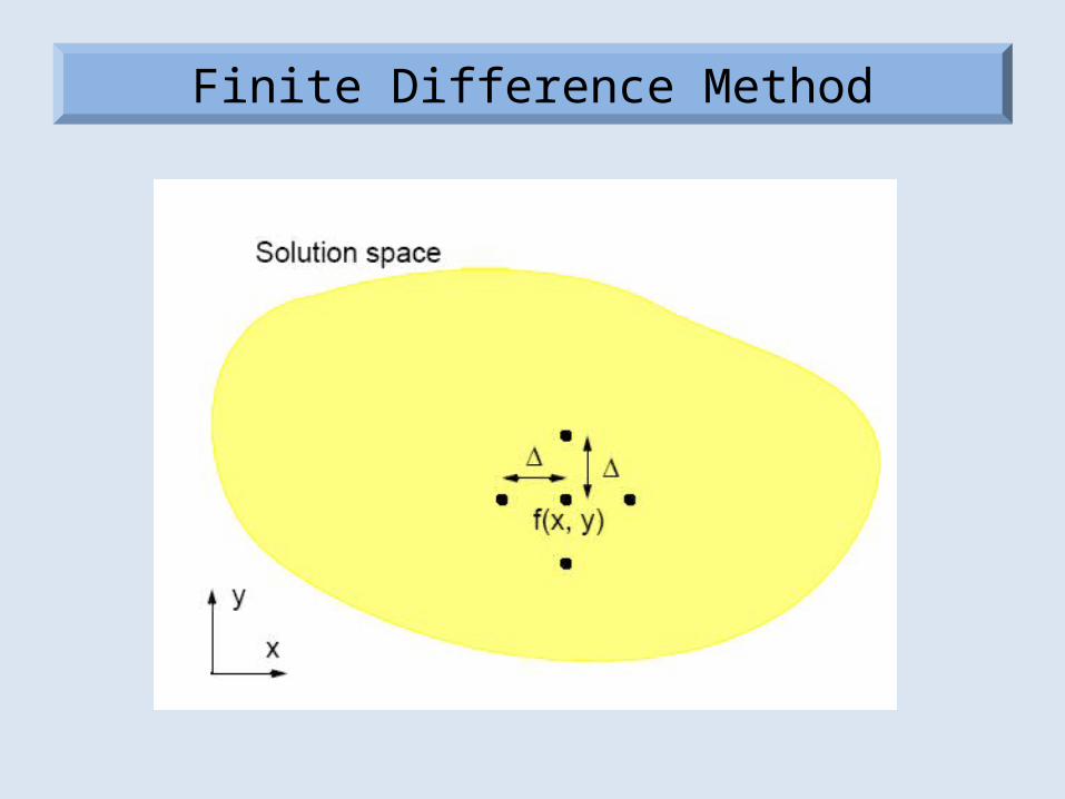
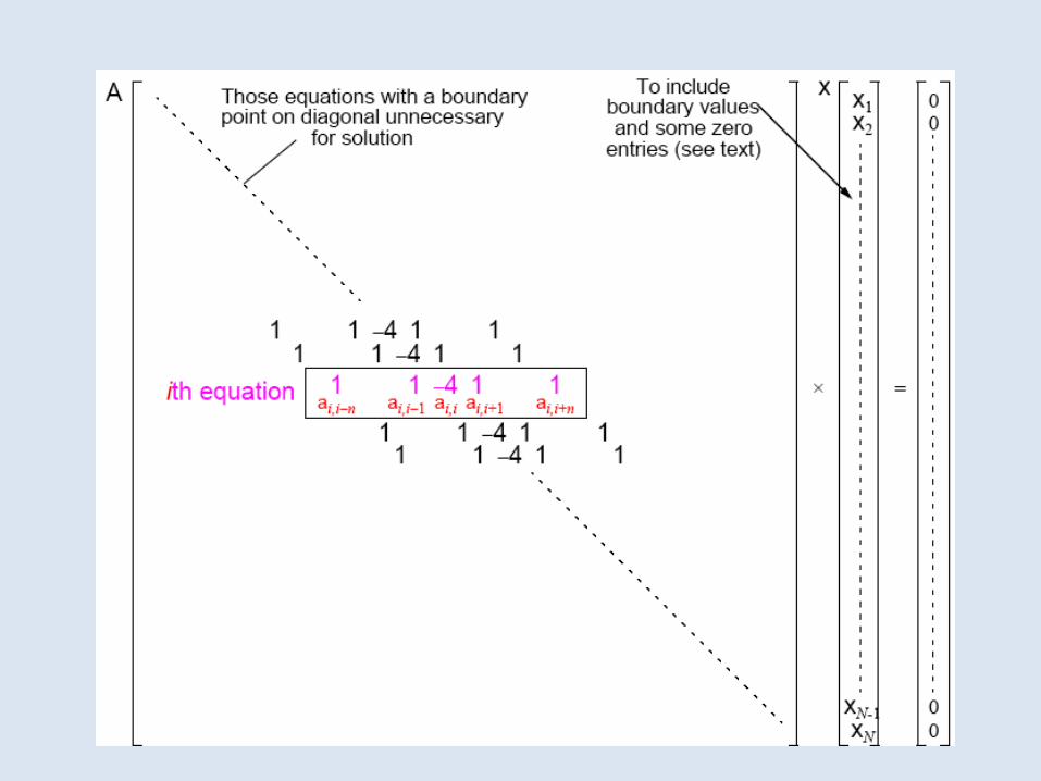
Finite Difference Method

First, black points computed simultaneously. Next, red points computed simultaneously.

Red-Black Ordering