nuclear geometries with weight-sharing deep neural networks

Solving the electronic Schrodinger equation for multiple

nuclear geometries with weight-sharing deep neural networks

Michael Scherbela†,*, Rafael Reisenhofer‡,a,*, Leon Gerard†,*, PhilippMarquetand†,§, and Philipp Grohs†,‡,¶

†Research Network Data Science @ Uni Vienna, Kolingasse 14-16, A-1090 Vienna, Austria‡Faculty of Mathematics, University of Vienna, Oskar-Morgenstern-Platz 1, A-1090 Vienna, Austria

§Faculty of Chemistry, University of Vienna, Wahringer Straße 17, 1090 Vienna, Austria¶Johann Radon Institute for Computational and Applied Mathematics, Austrian Academy of Sciences,

Altenbergerstrasse 69, 4040 Linz, [email protected]

*These authors contributed equally

Abstract

Accurate numerical solutions for the Schrodinger equation are of utmost importance inquantum chemistry. However, the computational cost of current high-accuracy methods scalespoorly with the number of interacting particles. Combining Monte Carlo methods with un-supervised training of neural networks has recently been proposed as a promising approachto overcome the curse of dimensionality in this setting and to obtain accurate wavefunctionsfor individual molecules at a moderately scaling computational cost. These methods cur-rently do not exploit the regularity exhibited by wavefunctions with respect to their moleculargeometries. Inspired by recent successful applications of deep transfer learning in machinetranslation and computer vision tasks, we attempt to leverage this regularity by introducinga weight-sharing constraint when optimizing neural network-based models for different molec-ular geometries. That is, we restrict the optimization process such that up to 95 percent ofweights in a neural network model are in fact equal across varying molecular geometries. Wefind that this technique can accelerate optimization when considering sets of nuclear geome-tries of the same molecule by an order of magnitude and that it opens a promising routetowards pre-trained neural network wavefunctions that yield high accuracy even across differ-ent molecules.

1 Introduction

Using a deep neural network-based ansatz for variational Monte Carlo (VMC) has recently emergedas a novel approach for highly accurate ab-initio solutions to the multi-electron Schrodinger equa-tion [1–5]. It has been observed that such methods can exceed gold-standard quantum-chemistrymethods like CCSD(T) [6] in accuracy, with a computational cost per step scaling only with O(N4)in the number of electrons [4]. This suggests a drastic improvement from classical quantum-chemistry methods such as CCSD(T), or CISDTQ1, which scale with O(N7) and O(N10), re-spectively. However, due to the large number of free parameters and the need for Monte Carlointegration, the constant prefactor for neural network-based methods is typically much larger thanfor classical approaches such that even systems of modest size still require days or weeks of compu-tation when using highly optimized implementations on state-of-the-art hardware [7]. This oftenrenders deep neural network (DNN)-based ansatz methods unfeasible in practice, in particularwhen highly accurate results for a large number of molecular geometries are required.

Among such tasks are computational structure search, determination of chemical transitionstates, and the generation of training datasets for supervised machine learning algorithms in quan-tum chemistry. Latter methods are applied with great success to interpolate results of established

1Configuration interaction singles, doubles, triples, quadruples

1

arX

iv:2

105.

0835

1v2

[ph

ysic

s.co

mp-

ph]

17

Dec

202

1

quantum chemistry methods such as energies and forces [8–10], properties of excited states [11],underlying objects such as orbital energies [12], or the exchange energy [13]. Given sufficient train-ing data, these interpolations already achieve chemical accuracy relative to the training method(e.g. Density Functional Theory) [14], highlighting the need for increasingly accurate ab-initiomethods which can be used to generate reference training data.

The goal of making DNN-based VMC applicable for the generation of such high-quality datasetsfor previously untractable molecules is a key motivation for this work. The apparent success ofsupervised learning in quantum chemistry suggests a high degree of regularity of the aforementionedproperties and the wavefunction itself within the space of molecular geometries.

Here, we aim to exploit potential regularities of the wavefunction within the space of moleculargeometries already during VMC optimization by applying a simple technique called weight-sharing.Throughout optimizing instances of the same neural network-based wavefunction model for dif-ferent molecular geometries, we enforce that for large parts of the model, each instance has theexact same neural network weights. In particular, this means that on the parts of the model whereweight-sharing is applied, each instance computes precisely the same function. We note that thisidea is reminiscent of (and inspired by) the ML technique deep transfer learning where parts of apre-trained model are reused for different similar tasks and which has led to breakthrough results,for example in natural language processing [15] or computer vision [16].

Weight-sharing can be viewed as a regularization technique which requires large parts of theoptimized model to work equally well for a potentially wide variety of different nuclear, or evenmolecular, geometries. Under the assumption that the wavefunctions are sufficiently regular acrossgeometries, it should therefore have a stabilizing effect on the optimization process and yieldwavefunctions that also generalize well to new molecular geometries when used as an initial guessbefore optimization. For a shared weight, each gradient descent update during optimization for aspecific geometry is applied to the complete set of considered geometries. Weight-sharing thereforehas the potential of significantly accelerating the optimization process.

Our main numerical results highlight the benefits of weight-sharing as compared to indepen-dent optimization (Sec. 2.1) and the applicability of pre-trained shared weights for new calcula-tions (Sec. 2.2). In particular, we show that by applying these techniques in combination withsecond-order optimization, it is possible to consistently reach the energies of MRCI-F12 referencecalculations – up to chemical accuracy – for molecules up to the size of ethene after only O(102) op-timization epochs per geometry. Note that for most recently proposed DNN-based VMC methods,wavefunctions are typically being optimized for O(104) - O(105) epochs. To further demonstratethe applicability of the proposed framework in practice, we calculate the transition path for H+

4 be-tween two symmetry equivalent minima, wavefunctions for a set of differently twisted and stretchedethene configurations, as well as the potential energy surface (PES) – including forces – of a H10

chain on a 2D grid of nuclear coordinates (Sec. 2.3). While nuclear forces are also available forother methods, such as domain-based local pair natural orbital (DLPNO)-Coupled-Cluster [17],they are not available for all types of systems [18], or come at a significant additional computationalcost, while our approach yields forces at a low incremental cost.

2 Results

To investigate weight-sharing for neural network-based models in VMC, we consider a framework,dubbed DeepErwin, where the trial wavefunction is modeled similar to the recently proposedPauliNet [2], with modifications leading to an overall smaller network that yields higher accuracies.The basic idea behind this model is to enhance a Slater determinant ansatz with deep neuralnetworks, where initial orbitals are obtained from a CASSCF (complete active space self-consistentfield) calculation with a small basis set and a small active space. The resulting wavefunction is thenmodified by applying a backflow transformation to the orbitals as well as to the electron coordinates,and via an additional Jastrow factor. All these enhancements depend on an embedding of theelectron coordinates into a high-dimensional feature space which takes into account interactionswith all other particles. This embedding is based on Electronic SchNet [19] and PauliNet. Cuspcorrection is performed explicitly [20]. In contrast to PauliNet, we use an additional equivariantbackflow shift for the electron coordinates, smaller embedding networks, and no residual in the

2

(a)

LiH Li2 Be B C H100

2

4

6

8

10

ener

gy e

rror /

mHa

DeepErwin w/o weight-sharing + KFAC(~110k parameters)DeepErwin w/o weight-sharing + Adam(~110k parameters)PauliNet + Adam(~150k parameters)

(b)

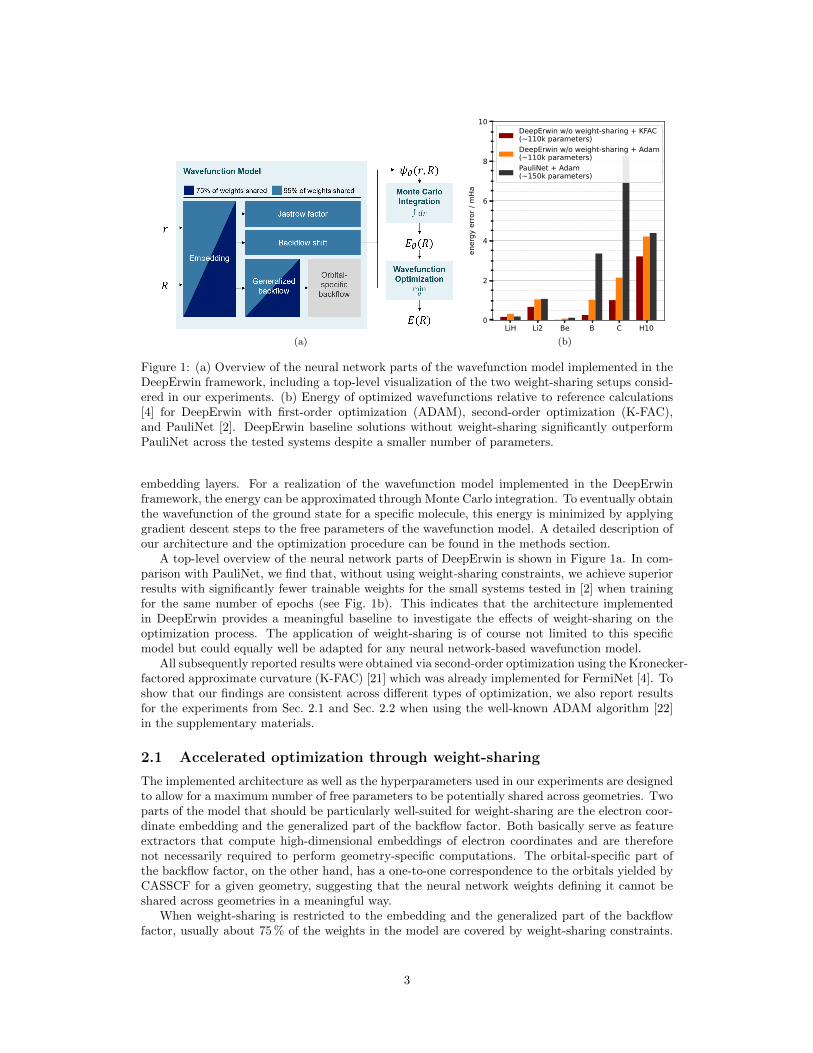
Figure 1: (a) Overview of the neural network parts of the wavefunction model implemented in theDeepErwin framework, including a top-level visualization of the two weight-sharing setups consid-ered in our experiments. (b) Energy of optimized wavefunctions relative to reference calculations[4] for DeepErwin with first-order optimization (ADAM), second-order optimization (K-FAC),and PauliNet [2]. DeepErwin baseline solutions without weight-sharing significantly outperformPauliNet across the tested systems despite a smaller number of parameters.

embedding layers. For a realization of the wavefunction model implemented in the DeepErwinframework, the energy can be approximated through Monte Carlo integration. To eventually obtainthe wavefunction of the ground state for a specific molecule, this energy is minimized by applyinggradient descent steps to the free parameters of the wavefunction model. A detailed description ofour architecture and the optimization procedure can be found in the methods section.

A top-level overview of the neural network parts of DeepErwin is shown in Figure 1a. In com-parison with PauliNet, we find that, without using weight-sharing constraints, we achieve superiorresults with significantly fewer trainable weights for the small systems tested in [2] when trainingfor the same number of epochs (see Fig. 1b). This indicates that the architecture implementedin DeepErwin provides a meaningful baseline to investigate the effects of weight-sharing on theoptimization process. The application of weight-sharing is of course not limited to this specificmodel but could equally well be adapted for any neural network-based wavefunction model.

All subsequently reported results were obtained via second-order optimization using the Kronecker-factored approximate curvature (K-FAC) [21] which was already implemented for FermiNet [4]. Toshow that our findings are consistent across different types of optimization, we also report resultsfor the experiments from Sec. 2.1 and Sec. 2.2 when using the well-known ADAM algorithm [22]in the supplementary materials.

2.1 Accelerated optimization through weight-sharing

The implemented architecture as well as the hyperparameters used in our experiments are designedto allow for a maximum number of free parameters to be potentially shared across geometries. Twoparts of the model that should be particularly well-suited for weight-sharing are the electron coor-dinate embedding and the generalized part of the backflow factor. Both basically serve as featureextractors that compute high-dimensional embeddings of electron coordinates and are thereforenot necessarily required to perform geometry-specific computations. The orbital-specific part ofthe backflow factor, on the other hand, has a one-to-one correspondence to the orbitals yielded byCASSCF for a given geometry, suggesting that the neural network weights defining it cannot beshared across geometries in a meaningful way.

When weight-sharing is restricted to the embedding and the generalized part of the backflowfactor, usually about 75 % of the weights in the model are covered by weight-sharing constraints.

3

64 256 1,024 4,096 16,384

0

1

2

3

4

5

6

ener

gy re

l. to

MRC

I / m

Ha ~6x

H +4 : 112 geometries

Independent opt.75% of weights shared95% of weights sharedChem. acc.: 1 kcal/mol

64 256 1,024 4,096 16,384

0

1

2

3

4

5

6

~8x

H6: 49 geometries

64 256 1,024 4,096 16,384training epochs / geometry

0

2

4

6

8

10

ener

gy re

l. to

MRC

I / m

Ha ~7x

H10: 49 geometries


0

5

10

15

20

25

30

~13x

Ethene: 30 geometries

Figure 2: Mean evaluation error relative to the reference calculation (MRCI-F12(Q)/cc-pVQZ-F12) as a function of training epochs per geometry for four different sets of nuclear geometries.Shadings indicate the area between the 25 % and the 75 % percentile of considered geometries. Foreach method, we plot intermediary and final results for optimizations that ran for a total numberof 16,384 epochs per geometry, respectively 8,192 epochs per geometry for shared optimization ofH10 and ethene. Note that for H10, the reference energies here differ slightly from the referenceenergy in Figure 1b, which was not available for the complete set of 49 geometries.

In the most extreme case, when all weights are being shared – except the ones defining the orbital-specific backflow – this number grows to roughly 95 % (cf. Fig. 1a). Note that precise counts forthe numbers of total and shared model parameters used for the experiments in this section slightlydiffer between different molecules (see Table 2).

We evaluate both these setups in four cases by computing the PES of four different molecules,namely H+

4 , the linear hydrogen chains H6 and H10, and ethene. For H+4 , we consider a diverse

set of 112 different configurations, covering both low-energy relaxed geometries, as well as stronglydistorted configurations. For both hydrogen chains, we calculate the wavefunction of the groundstate for 49 different nuclear geometries that lie on a regular grid with respect to a parametrizationbased on the distance a of two adjacent H-atoms and the distance x between these H2 pairs. Inthe case of twisted ethene, the set of 30 geometries iterates over ten different twist angles andthree different bond lengths for the carbon-carbon double bond. Figure 5a depicts the resultingPES for H10. Figure 4b plots the obtained energies for the minimum-energy-path from the non-twisted equilibrium geometry to the 90 rotated molecule, considering for each twist angle the CCbond-length with the lowest energy.

For all four molecules, we compare the optimization of the wavefunction models when applyingweight-sharing with the respective independent optimizations. The results of these experimentsare compiled in Figure 2. Across all physical systems, the optimization converges fastest when95 % of the weights are being shared. In particular, we find that in this case, the reference energy(MRCI-F12(Q)/cc-pVQZ-F12; see Methods section for computational details) can be reached, up

4

64 256 1,024 4,096 16,384

0

1

2

3

4

5

6

ener

gy re

l. to

MRC

I / m

Ha


Independent opt.Pre-trained by shared opt.Pre-trained by shared opt.of smaller moleculeChem. acc.: 1 kcal/mol

64 256 1,024 4,096 16,384

0

1

2

3

4

5

6H6: 23 geometries


0

2

4

6

8

10

ener

gy re

l. to

MRC

I / m

Ha

H10: 23 geometries


0

5

10

15

20

25

30Ethene: 20 geometries

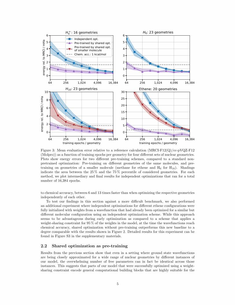
Figure 3: Mean evaluation error relative to a reference calculation (MRCI-F12(Q)/cc-pVQZ-F12(Molpro)) as a function of training epochs per geometry for four different sets of nuclear geometries.Plots show energy errors for two different pre-training schemes, compared to a standard non-pretrained optimization: Pre-training on different geometries of the same molecules, and pre-training on geometries of a smaller molecule (methane for ethene and H6 for H10). Shadingsindicate the area between the 25 % and the 75 % percentile of considered geometries. For eachmethod, we plot intermediary and final results for independent optimizations that ran for a totalnumber of 16,384 epochs.

to chemical accuracy, between 6 and 13 times faster than when optimizing the respective geometriesindependently of each other.

To test our findings in this section against a more difficult benchmark, we also performedan additional experiment where independent optimizations for different ethene configurations werefully initialized with weights from a wavefunction that had already been optimized for a similar butdifferent molecular configuration using an independent optimization scheme. While this approachseems to be advantageous during early optimization as compared to a scheme that applies aweight-sharing constraint for 95 % of the weights in the model, at the time the wavefunctions reachchemical accuracy, shared optimization without pre-training outperforms this new baseline to adegree comparable with the results shown in Figure 2. Detailed results for this experiment can befound in Figure S3 in the supplementary materials.

2.2 Shared optimization as pre-training

Results from the previous section show that even in a setting where ground state wavefunctionsare being closely approximated for a wide range of nuclear geometries by different instances ofour model, the overwhelming number of free parameters can in fact be identical across thoseinstances. This suggests that parts of our model that were successfully optimized using a weight-sharing constraint encode general computational building blocks that are highly suitable for the

5

approximation of different wavefunctions. In particular, one could hope that those building blocksalso generalize well to molecular geometries for which they were not previously optimized.

To test this hypothesis, we consider for each of the four molecules from the previous experimenta small new set of nuclear geometries that were not part of the original shared optimization. Forthese sets, we compare two types of independent optimization. In one case, a default randommethod is used to initialize the weights of the neural networks before optimization. In the secondcase, we reuse results from the previous optimization in the sense that all weights of the modelthat were shared in the first experiment are now initialized from the result of this optimization.For the remaining 5 % of weights, default random initialization is applied.

Pushing this approach even further, we also use previously optimized shared weights to initializewavefunction models for an entirely different molecule. In particular, we use shared weights thatwere optimized for the hydrogen chain H6 to initialize models for H10, and weights that wereoptmized for methane to initialize models for ethene. This is possible because the embeddingnetwork architecture is independent of the number of particles in the respective molecule. Ifsuccessful, this method can be used to pre-train weights for large and expensive molecules bysolving the Schrodinger equation for smaller, computationally cheaper systems.

The results of these experiments are shown in Figure 3. For all four considered molecules, weused weights that were optimized with a shared-weight constraint on a set of different geometries(cf. Fig. 2) for 8,192 optimization epochs per geometry. Across all systems, pre-training viashared optimization with different geometries of the same molecules dramatically accelerates thesubsequent optimization such that the reference energy can be consistently reached up to chemicalaccuracy after little more than a hundred optimization epochs. In the case of H10, the usage ofweights that were pre-trained on different configurations of a smaller molecule also yields significant,albeit much smaller improvements. When using methane configurations to pre-train a wavefunctionmodel for ethene, however, we could only find slight improvements during early optimization.

2.3 Calculating transition paths and forces

The significant speed-ups obtained through weight-sharing enable efficient computational studiesfor systems that consist of many different geometries of the same molecule. We demonstrate thecapabilities of our approach on two exemplary tasks: Finding transition paths and calculatingpotential energy surfaces. As a first example, we calculate the transition path for H+

4 between twosymmetry equivalent minima via a specific transition state previously proposed in the literature[23]. For all 19 points along the transition path, wavefunctions are optimized simultaneouslyfor 7,000 epochs per geometry using a weight-sharing constraint that covers about 95 % of totalweights in the model. We furthermore compute the energies along a reaction path for twistedethene which describes a rotation of the twist by 90. The ten geometries considered in this taskare a subsample of the 30 geometries previously used in the computations shown in Fig. 2. Asa baseline, we consider independent optimization without a weight-sharing constraint as well asclassical methods from computational chemistry.

The results of these calcualations are shown in Figure 4a and Figure 4b, respectively. We findour method to be in superior agreement with high-accuracy reference calculations: DeepErwin withweight-sharing predicts barrier heights that agree with MRCI within 1µHa (0.02%) for H+

4 , and 3.3mHa (3%) for ethene. This leads us to believe that the barrier height for H+

4 has been underesti-mated by approximately 1 mHa in previous high-accuracy calculations [23]. For the electronicallychallenging case of twisted ethene, both Hartree-Fock as well as CCSD(T)-F12 overestimate theenergy of the 90 twisted molecule. DeepErwin, however, yields barrier energies that are in muchcloser agreement with the MRCI-D-F12 calculations.

For calculating the transition paths, we used predefined sets of geometries as a given input.In many cases, however, it is not a-priori clear which nuclear geometries are of interest in a giventask, and a careful exploration of the respective PES is required. To do this efficiently, not onlyenergies, but also forces on the nuclei, that is, gradients of the energy with respect to the nuclearcoordinates, are required. For realizations of the DeepErwin wavefunction model, these forces canbe calculated in a straightforward and computationally efficient fashion via the Hellman-Feynmantheorem [24] and by applying established variance correction schemes to accelerate convergence ofthe Monte Carlo integration (see Methods section). The PES and the corresponding forces for the

6

0.0 0.2 0.4 0.6 0.8 1.0Reaction coordinate

0

1

2

3

4

5

6

7

8

ener

gy /

mHa

H +4

MRCI-D-F12Hartree-FockCCSD(T)-F12CAS AV7Z (Alijah 2008)DeepErwin w/o weight-sharingDeepErwin w/ weight-sharing

0 30 60 90Reaction coordinate

0

25

50

75

100

125

150

175

200

ener

gy /

mHa

Ethene

MRCI-D-F12Hartree-FockCCSD(T)-F12DeepErwin w/o weight-sharingDeepErwin w/ weight-sharing

(a)

0.0 0.2 0.4 0.6 0.8 1.0Reaction coordinate

0

1

2

3

4

5

6

7

8

ener

gy /

mHa

H +4

MRCI-D-F12Hartree-FockCCSD(T)-F12CAS AV7Z (Alijah 2008)DeepErwin w/o weight-sharingDeepErwin w/ weight-sharing

0 30 60 90Reaction coordinate

0

25

50

75

100

125

150

175

200

ener

gy /

mHa

Ethene

MRCI-D-F12Hartree-FockCCSD(T)-F12DeepErwin w/o weight-sharingDeepErwin w/ weight-sharing

(b)

Figure 4: (a) Energy of H+4 along reaction path between symmetry equivalent minima, via transi-

tion state 1 as defined in [23]. DeepErwin with weight-sharing constraints is in perfect agreementwith MRCI-F12(Q) and CCSD(T)-F12 after 7,000 optimization epochs per geometry. (b) Ener-gies for ten geometries that describe a rotation of the twist for twisted ethene by 90. Resultsfor DeepErwin with and without weight-sharing are plotted after 8,192 optimization epochs pergeometry.

linear hydrogen chain H10, evaluated on a regular grid of 49 geometries, are depicted in Figure 5aand Figure 5b, respectively. The corresponding wavefunctions were optimized for 8,192 epochs pergeometry using a weight-sharing constraint for approximately 95 % of the model weights. We findthat the energetic minimum is given by the dimerization into five H2 molecules with a covalentbond of a = 1.4 Bohr each, rather than for an equally spaced arrangement of atoms. This is aninstance of the well-known Peierls distortion [25].

Figure 5c shows that the force vectors obtained by DeepErwin via the Hellman-Feynman theo-rem are in perfect agreement with the forces computed from finite differences of MRCI-F12 refer-ence calculations. Our computational experiments do not show any signs of spurious Pulay forces[26], which occur when the approximated wavefunction is not an eigenfunction of the Hamiltonian.This suggests that DeepErwin yields not only highly accurate energies, but also highly accuratewavefunctions.

3 Discussion

Sharing the weights of realizations of a neural network-based wavefunction model across differ-ent nuclear geometries can significantly reduce the computational cost of VMC optimization. Forseveral molecules, we found that weight-sharing can in fact decrease the number of required op-timization epochs per geometry to reach a given reference energy up to chemical accuracy by afactor between 6 and 13. Our approach yields the best results when an overwhelming majorityof network weights is being shared, suggesting a strong regularity of wavefunctions of the consid-ered molecules within the space of nuclear geometries. Further evidence for this regularity is alsoprovided by a concurrent method named PESNet, which was released shortly after DeepErwinwas first available as a preprint [27]. PESNet is based on the FermiNet model and employs ameta graph neural network (GNN) to simultaneously learn wavefunctions for a complete potentialenergy surface (PES) such that after optimization, the model parameters for a new geometry canbe predicted via a simple forward pass through the meta GNN. The fact that this approach reli-ably yields high-accuracy results for different configurations that were sampled from a PES further

7

1.2 1.4 1.6 1.8a / bohr

1.6

1.8

2.0

2.2

2.4

2.6

2.8

x / b

ohr

0.5 0.0 0.5Force by MRCI-D-F12 / atomic. units

0.4

0.2

0.0

0.2

0.4

0.6

0.8

Forc

e by

Dee

pErw

in /

atom

ic. u

nits

Fx: (r2=0.999)Fa: (r2=1.000)

a / bohr1.8 1.6 1.4 1.2

x / bohr

1.62.0

2.42.8

E / Ha

5.8

5.7

5.6

5.5

(a)

1.2 1.4 1.6 1.8a / bohr

1.6

1.8

2.0

2.2

2.4

2.6

2.8

x / b

ohr


0.4

0.2

0.0

0.2

0.4

0.6

0.8

Forc

e by

Dee

pErw

in /

atom

ic. u

nits

Fx: (r2=0.999)Fa: (r2=1.000)

a / bohr1.8 1.6 1.4 1.2

x / bohr

1.62.0

2.42.8

E / Ha

5.8

5.7

5.6

5.5

(b)

1.2 1.4 1.6 1.8a / bohr

1.6

1.8

2.0

2.2

2.4

2.6

2.8

x / b

ohr


0.4

0.2

0.0

0.2

0.4

0.6

0.8

Forc

e by

Dee

pErw

in /

atom

ic. u

nits

Fx: (r2=0.999)Fa: (r2=1.000)

a / bohr1.8 1.6 1.4 1.2

x / bohr

1.62.0

2.42.8

E / Ha

5.8

5.7

5.6

5.5

(c)

Figure 5: (a) Potential energy surface (PES) for the H10 chain. The variable a is representingthe distance between two H-atoms and x is the distance between two H2 molecules. The lowestground state of the PES describes the dimerization. (b) Cubic interpolation of the PES withforce vectors for the H10 chain. Red arrows depict force vectors computed by DeepErwin via theHellmann-Feynman theorem, whereas black arrows represent numerical gradients that are based onfinite differences of MRCI-F12 reference calculations. (c) Forces computed by DeepErwin plottedagainst the respective forces obtained from finite differences of the MRCI-F12 reference calculation.

underlines our observation that the regularity of wavefunctions within the space of geometries canbe heavily exploited for DNN-based QMC methods by also enforcing regularity on large domainsof the parameter space.

We found that optimized shared weights yield highly applicable initial weights when consid-ering nuclear geometries for which the wavefunction model was not previously optimized. Evenfor molecules such as ethene, pre-training with shared optimization makes it possible to reachan MRCI-F12(Q)/cc-pVQZ-F12 reference calculation up to chemical accuracy after only a fewhundred optimization epochs. A possibly attractive route towards making VMC optimizationtractable for more complex molecules could be to pre-train large parts of a wavefunction modelon small, computationally cheap, systems. In our experiments, we found that the optimizationof H10 wavefunctions can in fact be improved significantly when using shared optimization fora set of H6 geometries to pre-train the respective models. In the case of ethene, however, wecould only see small improvements during early optimization when parts of the respective modelwere pre-trained on sets of smaller methane geometries. Due to the fact that any optimization ofDNN-based wavefunction models is highly sensitive to changes in the architecture and optimiza-tion hyperparameters, we would consider our findings as preliminary evidence that merits furtherresearch towards the development of a kind of universal wavefunction, whose neural network partswere optimized for a great number of diverse molecular geometries and which is therefore capableof closely of approximating wavefunctions of the ground state for many physical systems after onlya brief step of additional optimization.

Our results do not provide a conclusive answer whether for the investigated sets of moleculargeometries, the considered weight-sharing setups actually limit the capability of our model toapproximate the true wavefunctions of the ground state. In general, we would expect this tobe the case, but judging from our experimental results, the loss of expressiveness introduced byweight-sharing regularization might often be negligible. This is evidenced by the fact that acrossall experiments, sharing 95 % of model weights yields the same or even lower energies than therespective independent optimizations. It is furthermore not clear yet, what an optimal algorithmthat exploits weight-sharing for a given task could look like. Based on our results so far, for anexhaustive study of the PES of a molecule, we would suggest a procedure where – possibly guidedby estimates of the forces on the nuclei – geometries of interest are iteratively included in a sharedoptimization, and which is eventually concluded by an additional step of independent optimizationfor some or all of the considered geometries.

The proposed method of weight-sharing is not limited to the specific architecture used in this

8

work but could potentially be exploited for any neural network-based wavefunction model. Dueto the interesting regularization properties, it could even be beneficial to apply weight-sharing ina context where only the wavefunction for a single molecular geometry is of interest.

A potential drawback of the proposed method in practice is that shared optimization cannot easily be parallelized across multiple devices (GPUs or CPUs), because each geometry isdependent on updates from all other geometries. One possibility to overcome this issue would beto consider an average loss across all geometries during gradient descent. Such a loss could easilybe parallelized by using a separate device for each geometry. In our current implementation ofthe DeepErwin framework, however, for each epoch only a single geometry is considered duringshared optimization, and it is therefore only possible to distribute the Monte Carlo samples withina batch across multiple devices, as it is common practice [7].

4 Methods

For a molecule with nnuc nuclei, n↑ spin-up electrons, and n↓ spin-down electrons, we writer = (r1, . . . , rn↑ , . . . , rn↑+n↓) to denote the set of Cartesian electron coordinates, and R =(R1, . . . , Rnnuc

) for the set of coordinates of nuclei. The electron coordinates r are always as-sumed to be ordered such that the first n↑ entries correspond to spin-up electrons, while the lastn↓ entries are coordinates of spin-down electrons. We write nel = n↑ + n↓ for the total number ofelectrons and Zi for the charge of the i-th nucleus.

4.1 Wavefunction model

The model implemented in DeepErwin is closely related to the recently proposed PauliNet [2].Let θ denote the set of all free (trainable) parameters in the model and ndet the numberof enhanced Slater determinants. With a high-dimensional embedding of electron coordinatesx(r;R) = (x1, . . . , xn↑ , . . . , xn↑+n↓) and an explicit term γ(r) for cusp correction in the Jastrowfactor, a realization ψθ of the DeepErwin wavefunction model can be written as

ψθ(r) = eJ(x(r;R))+γ(r)ndet∑

d=1

αd det[Φ↑d (r,x(r;R))

]det[Φ↓d (r,x(r;R))

], (1)

where αd ∈ R is a trainable weight, the scalar function J defining the Jastrow factor is representedby two fully connected feedforward neural networks, and Slater determinants for spin-up electronsare defined via

Φ↑d (r,x(r;R)) =

ϕ↑,d1

(r1 + s1(r,x;R)

)η↑,d1 (x1) · · · ϕ↑,d1

(rn↑ + sn↑(r,x;R)

)η↑,d1 (xn↑)

.... . .

...ϕ↑,dn↑

(r1 + s1(r,x;R)

)η↑,dn↑ (x1) · · · ϕ↑,dn↑

(rn↑ + sn↑(r,x;R)

)η↑,dn↑ (xn↑)

. (2)

Matrices Φ↓d (r,x(r;R)) for spin-down electrons can be defined analogously. The single electron

orbitals ϕ↑,di are obtained from the ndet most significant Slater determinants from a CASSCFmethod and remain fixed throughout optimization. The backflow shifts si as well as the backflowfactors η↑,di are represented by fully connected feedforward neural networks. The embedded coor-dinate xi of the i-th electron takes into account all particle positions in the system independent ofparticle type and spin. An overview of the model given by eq. (1) is shown in Figure 6. Furtherdetails regarding our implementation of the coordinate embedding, the Jastrow factor, backflowtransformation, as well as cusp correction are given below.

4.1.1 Electron coordinate embedding

The embedding x(r;R) is a slightly simplified version of the SchNet embedding used for PauliNet[2, 19]. For brevity, we extend our notation to also include the nuclear coordinates in the coor-dinates rj by defining rj = Rj−nel

for nel < j ≤ nnuc. To embed the coordinates ri of the i-thelectron, we consider input features based on pairwise differences and distances with respect to allother particles in the system. Let i ∈ 1, . . . , nel, j ∈ 1, . . . , nel + nnuc, and nrbf denote the

9

Figure 6: Overview of the computational architecture implemented in DeepErwin. Spin depen-dance has been omitted for clarity, but in practice there are two parallel streams for spin-up andspin-down respectively.

number of radial basis features. We use #»r ij = ri−rj , and rij = | #»r ij | to denote pairwise differencesand distances, respectively, and define the pairwise feature vector

hij =

(e−(rij−µ1)2/σ2

1 , . . . , e−(rij−µnrbf)2/σ2

nrbf ,1

rij + 0.01

)∈ Rnrbf+1+3, (3)

where the mean and variance parameters are defined as

µk = cq2k, and σk =

1

7(1 + cqk), (4)

respectively, for an index k ∈ 1, . . . , nrbf, a parameter qk that is chosen from an equidistant gridof the interval [0, 1], and a cutoff parameter c ∈ R.

For a fixed integer L and an embedding dimension nemb, let(gl, wlsame, w

lop, w

lnuc

)Ll=0

and(f lsame, f

lop

)Ll=1

denote sequences of vector-valued functions, where each function is representedby a fully connected feedforward neural network with output dimension nemb. To embed thecoordinates of the i-th electron based on the pairwise feature vectors hij , we use to denoteelement-wise multiplication and define for i ∈ 1, . . . , nel

x0i = g0

nel∑

j=1j 6=i

w0σij

(hij) f0σij

+

nel+nnuc∑

j=nel+1

w0nuc(hij) f0

Zj−nel

, (5)

xli = gl

nel∑

j=1j 6=i

wlσij(hij) f lσij

(xl−1j ) +

nel+nnuc∑

j=nel+1

wlnuc(hij) f lZj−nel

with 1 ≤ l ≤ L, (6)

where σij = ’same’ for same-spin pairs of electrons and σij = ’op’ for pairs of electrons withopposite spin, and where f0

same, f0op, and f0

Zj−nel, . . . , fLZj−nel

denote trainable vectors of length

nemb. The embedding of the i-th electron coordinates ri is eventually defined as

xi = xLi . (7)

10

The embedding originally applied in PauliNet has an additional residual term in eq. (6) and

considers specific functions(gl)Ll=0

for same-spin, opposite-spin, and nuclear input channels.

4.1.2 Backflow transformation

Based on the embedding x(r;R), our model applies spin-dependent backflow shifts and factors tothe single electron orbitals in the Slater determinants (cf. eq. (2)). For simplicity, this section onlyconsiders the spin-up case.

Let η↑gen denote a vector-valued function that is represented by a fully connected feedforwardneural network, and ωbf ∈ R a single spin-independent trainable weight. For the i-th orbital andthe j-th electron in the d-th Slater determinant, the backflow factor is computed as

η↑,di (xj) = 1 + ωbfη↑,di

(η↑gen(xj)

), (8)

where η↑,di denotes an orbital-specific function that is also represented by a feedforward neuralnetwork.

The inner function η↑gen can be seen as an extension of the embedding layer. Apart fromelectron spin orientation, it remains unchanged across electrons and determinants and is hencecalled general backflow factor. The outer function η↑,di , on the other hand, is specific to the i-thorbital in the d-th determinant obtained from a CASSCF method. The motivation behind definingthe backflow factor via the composition of these two functions was to maximize the number ofneural networks weights than can possibly be shared across nuclear geometries. Note that for twodistinct nuclear geometries, CASSCF does in general not yield the same number of unique orbitals.While this does not raise an issue for the general backflow factor η↑gen, it implies that sharing the

neural network weights that define η↑,di across nuclear geometries is in general not possible in ameaningful way.

Based on ideas from [28], the backflow shift is based on rotation-invariant features and rotation-equivariant pairwise differences. It is furthermore split into an electron-electron and an electron-nucleus part. Besides the embedding, we additionally use side products of the embedding networkas inputs and define the following feature vectors

f eli =

(wLσi1

(hi1) fLσi1(xL−1

1 ), . . . , wLσinel(hinel

) fLσinel(xL−1nel

))

(9)

and

fnuci =

(wLnuc(hi(nel+1)) fLZ1

, . . . , wLnuc(hi(nel+nnuc)) fLZnnuc

)(10)

for i ∈ 1, . . . , nel. All features are obtained without additional cost at the end of the embeddingloop (cf. 6). The electronic part of the shift for the i-th electron is defined as

seli (r, xi, f

eli ) =

nel∑

k=1k 6=i

sel

(xi, f

eli

) #»r ik1 + r3

ik

. (11)

In contrast to the backflow factor, we do not differentiate between different spins to reduce com-plexity. Similarly, the electron-nuclear shift is computed via

snuci (r,R, xi, f

nuci ) =

nnuc+nel∑

k=nel+1

snuc

(xi, f

ioni

) #»r ik1 + r3

ik

, (12)

where sel and snuc are represented by feed-forward neural networks. A decay in the vicinity ofnuclei ensures that the applied backflow shifts do not lead to a violation of the Kato cusp condition[29]. The complete backflow shift is computed by

si(r,R, xi, feli , f

nuci ) = ωsh

∏

n

tanh (2Zn|ri −Rn|)2(seli (xi, f

eli ) + snuc

i (xi, fnuci )

), (13)

with a spin-independent trainable weight ωsh ∈ R.

11

4.1.3 Jastrow factor

With two spin-dependent scalar functions J↑ and J↓, that are both represented by fully connectedfeedforward neural networks, the Jastrow factor (cf. eq. (1)) is defined as

J (x(r;R)) =

n↑∑

i=1

J↑(xi) +

nel∑

i=n↑+1

J↓(xi). (14)

4.1.4 Cusp correction

The Kato cusp condition [29] is a necessary condition for eigenstates of the Hamiltonian H. Itensures that the local energies of a wavefunction ψ are finite by forcing the kinetic energy term∇2ψ to diverge in such a way that it exactly cancels the divergence caused by the potentialenergy term Zn/|ri − Rn| when the i-th electron approaches the n-th nucleus. The orbitals ϕ↑,di ,

respectively ϕ↓,di , yielded by a CASSCF method (cf. eq. 2), do in general not lead to enhancedSlater determinants that satisfy the cusp condition. To address this issue, we follow the approachoutlined in [20]: Within a radius Rcusp around the nuclei, we replace the molecular orbitals byan exponentially decaying function which satisfies the Kato cusp condition, transitions smoothlyinto the orbitals at Rcusp, and minimizes the variance of the local energy of this orbital. Cuspcorrection for the enhanced Slater determinants is performed after the initial set of orbitals has beenobtained from a CASSCF calculation and remains fixed during the optimization of the wavefunctionparameters θ.

To account for electron-electron cusps in the Jastrow factor (cf. eq. 1), we use an explicit term

γ(r) =

nel∑

i=1

nel∑

j=i+1

rijrij + 1

, (15)

similar to the one applied in [1].

4.2 Variational Monte Carlo

We use a standard variational Monte Carlo approach to optimize our wavefunction ansatz. Let

H = Ekin + Epot (16)

denote the electronic Hamiltonian as obtained within the Born-Oppenheimer approximation, with

Ekin = −1

2

∑

i

∇2ri , (17)

Epot =∑

i>j

1

|ri − rj |+∑

n>m

ZnZm|Rn −Rm|

−∑

i,n

Zn|ri −Rn|

, (18)

where Ekin accounts for the kinetic energy of the electrons, and Epot accounts for the attractionand repulsion between particles in the system. By the Rayleigh-Ritz variational principle, it holdsfor any wavefunction ψθ that its energy Eθ is greater than or equal to the ground state energy E0

of the eigenfunction of H associated to the smallest eigenvalue, that is

Eθ =

∫ψθ(r)Hψθ(r)

Ωθdr ≥ E0, (19)

where Ωθ =∫ψθ(r)2dr denotes a normalization factor.

To evaluate the energy Eθ for a given set of parameters θ, we use Markov chain Monte Carlointegration (MCMC) and sample electron coordinates according to the probability density

pθ(r) =ψθ(r)2

Ωθ. (20)

12

This allows us to express the total energy Eθ as the expected value of a local energy

Eloc(r) =Hψθ(r)

ψθ(r), (21)

in the sense that

Eθ =

∫Eloc(r)pθ(r)dr = 〈Eloc〉 ≈

1

N

N∑

k=1

Eloc(rk), (22)

where N denotes the number of sampled electron coordinates and rk ∼ pθ.To optimize the parameters θ, we use K-FAC [21] which was already implemented in FermiNet

[4] to minimize the local energy Eloc(rk) at the location of electron coordinates rk. DeepErwinalso supports the limited-memory Broyden–Fletcher–Goldfarb–Shanno algorithm (L-BFGS [30]),which is another second-order method, as well as standard first-order stochastic gradient descent(SGD) as implemented by the ADAM algorithm [22]. After each optmization epoch, that is, aftereach sample of coordinates was used exactly once for a gradient descent step, the coordinates rk areresampled to reflect the updated probability distribution pθ. By applying this procedure iterativelyfor a large number of epochs, we eventually obtain parameters θ such that the wavefunction ψθclosely approximates the wavefunction of the ground state for the considered molecule.

To increase numerical stability, the implementation of our ansatz does not directly model ψθ,but the logarithm of its square. The local energy can then be computed as

Eloc(r) = Epot(r)− 1

4∇2

rφθ(r)− 1

8(∇rφθ)

2(r), (23)

where φθ = log(ψ2θ).

Although the local energy already contains second derivatives (with respect to r), calculatingthe gradient with respect to θ does not require the calculation of third derivatives, because H isHermitian [31]. Precisely, it holds that

∇θEθ = 〈Eloc∇θφθ〉 − 〈Eloc〉〈∇θφθ〉 (24)

≈ 1

N

N∑

k=1

Eloc(rk)∇θφθ(rk)− 1

N2

(N∑

k=1

Eloc(rk)

)(N∑

k=1

∇θφθ(rk)

), (25)

for N samples of electron coordinates rk ∼ pθ.To approximate the distribution of electron coordinates defined by the density pθ, we typically

use about 2k independent MCMC chains (walkers), where each walker is initialized before opti-mization with a large number (∼ 1k) of burn-in steps. During optimization, walkers are updatedafter every epoch with a small number (∼ 10) of additional MCMC steps. To precisely estimatethe energy Eθ after optimization has concluded, we apply a similar procedure, but collect the localenergies for all walkers from roughly 1k intermediate steps in the respective MCMC chain.

For single steps in the MCMC chains, we use a Metropolis Hastings algorithm [32]. Given acurrent walker state r, a proposal state rprop for the Metropolis Hastings algorithm is generatedaccording to the probability density

p(rprop|r) =

nel∏

i=1

pN(rpropi |µ = ri, σ

2 = (di)2), (26)

where pN denotes the density of a three-dimensional normal distribution and the variance param-eters di are defined for fixed parameters d0, dmin, dmax, δ ≥ 0 as

di = δmin

(dmin +

|ri −Rn|d0

, dmax

), (27)

where Rn denotes the position of the nucleus closest to ri, that is, n = argminj=1,...,nnuc|ri −Rj |.

We then consider the canonical acceptance probability

pacc(rprop|r) = min

1,p(r|rprop)pθ(r

prop)

p(rprop|r)pθ(r)

, (28)

13

and for a sample α ∈ [0, 1] from a uniform distribution, the proposed sample rprop is accepted inthe case pacc(rprop|r) > α and rejected otherwise.

The parameters di defined in eq. (27) can be seen as step size parameters that regulate theaverage distance between electron coordinates r and a proposal rprop. In general, smaller stepsizes lead to higher acceptance rates for proposed samples. The parameter δ is a general step sizeparameter that is gradually adapted during optimization to yield an average acceptance rate of50%. The second factor in eq. (27) was specifically designed to take into account that wavefunctionsare usually most complex in the proximity of a nucleus. That is, the step size di is chosen for eachelectron i to depend on its distance to the closest ion to encourage smaller steps close to the nuclei,where the wavefunction varies rapidly, and larger steps, when an electron is further away from thenuclei.

Note that the step sizes di, and thus the proposal probability, depend on the electron positionsr. In general it is therefore not true that p(rprop|r) = p(r|rprop). However, due to our choice forthe acceptance probability pacc, the so-called detailed balance condition is still satisfied. That is,being in a state r and transitioning to rprop is as probable as being in rprop and transitioning tor.

4.3 Forces

For a given molecule, let ψ0 denote the wavefunction of the ground state, that is, ψ0 is the eigen-function of the Hamiltonian H associated to the smallest eigenvalue. To calculate the electronicforces acting on the m-th nuclei, we apply the Hellmann-Feynman theorem [24] and compute

Fm = −∇RmE0 = − 1

Ω0

∫ψ0(r) ((∇RmH)ψ0)(r)dr (29)

= Zm1

Ω0

∫ψ0(r)2

(∑

i

ri −Rm|ri −Rm|3

)dr −

∑

n 6=mZn

Rn −Rm|Rn −Rm|3

(30)

≈ Zm

1

N

∑

k

∑

i

rki −Rm|rki −Rm|3

−∑

n 6=mZn

Rn −Rm|Rn −Rm|3

, (31)

for N samples of electron coordinates rk ∼ ψ0(r)2/Ω0, and where Ω0 =∫ψ0(r)2dr denotes the

L2-norm of ψ0.Since it is no longer necessary to compute derivatives of the wavefunction, evaluating eq. (31)

should be relatively easy. However, unlike the local energy (cf. eq. (22)), which has zero variancefor eigenstates of the Hamiltonian, naive Monte Carlo sampling can not be applied in this case dueto the divergence of |ri −Rk|−3 when the i-th electron approaches the k-th nucleus.

This issue can be addressed by observing that for each diverging term on one side of a nucleus,there is an equally diverging term with the opposite sign on the other side of the nucleus. Differentvariance reduction methods have been proposed to exploit this property, such as fitting the forcedensity close to a nucleus with a function that is constrained to be zero at ri = Rk [33], or antitheticsampling [33, 34].

We minimize the variance of force samples by combining antithetic sampling with a truncated1/r potential: For each sample of electron coordinates rk yielded by a Markov chain, we alsoconsider an additional sample rk in which each electron within a distance of Rcore to the closestnucleus is mirrored to the opposite side of this nucleus.

rk,i = rki + 2(Rm − rki ) (32)

for i ∈ 1, . . . , nel, and m = argminn |ri − Rn|. Therefore, whenever an electron comes closeto a nucleus and thus generates a large force in one direction, there will always be a cancellingcontribution in the opposite direction. Note that the samples rk,i do not necessarily have thesame probability as the original sample rk. Their contribution to the Monte Carlo estimate is thus

weighted by ψ(rk,i)2

ψ(rk)2. Additionally we avoid numerical instabilities by replacing the raw Coulomb

14

forces with a scaled version that decays towards zero, as electrons approach a nucleus:

rki −Rm|rki −Rm|3

−→ rki −Rm|rki −Rm|3

tanh3

( |rki −Rm|Rcut-off

)(33)

4.4 Shared optimization of model parameters

For N distinct nuclear geometries R1,R2, . . . ,RN , let θsh denote the set of model parametersthat are shared across all geometries, and θk denote the set of parameters that are specific to thek-th set of nuclear coordinates Rk. The full set of parameters for the k-th geometry can thenbe written as θk = (θsh, θk), and the associated realization of the wavefunction model is denotedby ψθk . During each shared optimization epoch, we consider a single nuclear geometry Rk andupdate the respective model weights θk with respect to the local energies of the wavefunction ψθkat MCMC walker positions that were sampled from the probability density pθk (cf. eq. (20)). Thatis, during each shared optimization epoch, not only the geometry-specific weights are updated, butalso the shared weights θsh, and therefore the wavefunctions for all nuclear geometries.

A straightforward way of deciding which geometry to consider for a shared optimization epoch isto employ a simple round-robin scheme. Note that for each eigenstate of the Hamiltonian, the localenergies defined in eq. (21) have zero variance. Therefore, another approach to select geometriesfor a shared optimization epoch is to use the standard deviation of local energies as a proxy ofhow closely a realization of the wavefunction model already approximates the wavefunction ofthe ground state. By selecting the geometry for which the current wavefunction has the higheststandard deviation in the local energies, we ensure that geometries for which the parameters havenot yet been well optimized get more attention during optimization. In practice, we train a fewinitial epochs using the round-robin scheme to obtain a reliable starting point for each wavefunctionand then switch to the standard-deviation-based scheme, to ensure homogeneous convergence ofthe accuracy across all geometries.

In our implementation of the shared optimization scheme, we use a single instance of theoptimizer to update the set of shared weights θsh, as well as an additional instance for each of thegeometry-specific sets of model parameters. In particular, due to the fact that geometry-specificweights receive significantly less gradient descent updates than shared weights, the learning ratefor the geometry-specific optimizers are usually chosen about 10 times larger than the learningrate for the optimizer of the shared weights (cf. Table 1).

After the shared optimization process, the wavefunctions can again be treated as fully indepen-dent realizations of our wavefunction model and are not constrained by any additional dependen-cies. In particular, this means that the evaluation of their exact energy can easily be parallelizedacross geometries.

4.5 Reference calculations

In order to validate our deep learning method, we compared the obtained energies to referencevalues, which we computed using the MOLPRO package [35, 36]. We employed both single-and multi-reference explicitly correlated F12 methods: Coupled cluster with singles, doubles andperturbative triples (CCSD(T)-F12) [37] and multi-reference configuration interaction (MRCI-F12)[38]. The basis set cc-pVQZ-F12 [39] was used for all geometries of H+

4 , H6, and C2H4. Due toconvergence issues with this basis set for some geometries of H10, the smaller cc-pVTZ-F12 basisset was employed for this molecular system. For the MRCI-F12 calculations, a CASSCF referencewas used with a full-valence active space (H+

4 : 3 electrons in 3 orbitals abbreviated as (3, 3), H6:(6,6), H10: (10,10)). A full-valence active space was prohibitively expensive for C2H4, which is whywe resorted to an active space of (2,2). The recommended GEM BETA coefficients were used (i.e.,for MRCI-F12(Q)/cc-pVQZ-F12 calculations GEM BETA = 1.5 a−1

0 and for MRCI-F12(Q)/cc-pVTZ-F12 calculations GEM BETA = 1.4 a−1

0 ) [40]. The Davidson-corrected [41] energy values(MRCI-F12(Q)) were extracted, as provided by the energyd variable in MOLPRO.

We note that these accurate methods and basis sets were only used to validate our results, butnot as a starting point for our deep learning method. The orbitals used as a starting point for ourmethod were generated using the CASSCF method implemented in PySCF [42], using a 6-311GPople basis set.

15

4.6 Computational settings for DeepErwin

Reference values for the results shown in Fig. 2 were obtained via MRCI-F12(Q)/cc-pVQZ-F12.See Sec. 4.5 for more details.

In all cases, we used as reference the described method from section 4.5. However, for theinitialization from the H10 run two geometries were excluded from the reference set, since thesewere also included in the pre-trained geometry grid.

The main hyperparameters used for all computations are listed in Table 1. Detailed countsof total, trainable, and shared parameters for the used wavefunction models for the four mainmolecules considered in our numerical experiments are compiled in Table 2.

The DeepErwin package alongside a detailed documentation is available on the Python PackageIndex (PyPI) and github (https://github.com/mipunivie/deeperwin).

5 Acknowledgements

L.G. gratefully acknowledges support from the Austrian Science Fund (FWF I 3403) and theWWTF (ICT19-041). R.R. gratefully acknowledges support from the Austrian Science Fund (FWFM 2528). The computational results presented have been achieved using the Vienna ScientificCluster (VSC).

References

1. Han, J., Zhang, L. & E, W. Solving many-electron Schrodinger equation using deep neuralnetworks. J. Comput. Phys. 399, 108929. issn: 0021-9991. http://dx.doi.org/10.1016/j.jcp.2019.108929 (Dec. 2019).

2. Hermann, J., Schatzle, Z. & Noe, F. Deep-neural-network solution of the electronicSchrodinger equation. Nat. Chem. 12, 891–897. issn: 1755-4349. https://doi.org/10.1038/s41557-020-0544-y (Oct. 2020).

3. Manzhos, S. Machine learning for the solution of the Schrodinger equation. Mach. learn.: sci.technol. 1, 013002. https://doi.org/10.1088/2632-2153/ab7d30 (Apr. 2020).

4. Pfau, D., Spencer, J. S., Matthews, A. G. D. G. & Foulkes, W. M. C. Ab initio solution of themany-electron Schrodinger equation with deep neural networks. Phys. Rev. Res. 2, 033429.https://link.aps.org/doi/10.1103/PhysRevResearch.2.033429 (3 Sept. 2020).

5. Wilson, M., Gao, N., Wudarski, F., Rieffel, E. & Tubman, N. M. Simulations of state-of-the-art fermionic neural network wave functions with diffusion Monte Carlo 2021. arXiv:2103.12570 [physics.chem-ph].

6. Bartlett, R. J. & Musia l, M. Coupled-cluster theory in quantum chemistry. Rev. Mod. Phys.79, 291–352. https://link.aps.org/doi/10.1103/RevModPhys.79.291 (1 Feb. 2007).

7. Spencer, J. S., Pfau, D., Botev, A. & Foulkes, W. M. C. Better, Faster Fermionic NeuralNetworks. arXiv: 2011.07125 [physics.comp-ph] (2020).

8. Unke, O. T. et al. Machine Learning Force Fields. Chem. Rev. issn: 0009-2665. https :

//doi.org/10.1021/acs.chemrev.0c01111 (Mar. 2021).

9. Behler, J. Four Generations of High-Dimensional Neural Network Potentials. Chem. Rev.,DOI:10.1021/acs.chemrev.0c00868 (2021).

10. Kirkpatrick, J. et al. Pushing the frontiers of density functionals by solving the fractionalelectron problem. Science 374, 1385–1389. eprint: https://www.science.org/doi/pdf/10.1126/science.abj6511. https://www.science.org/doi/abs/10.1126/science.abj6511(2021).

11. Westermayr, J. & Marquetand, P. Machine Learning for Electronically Excited States ofMolecules. Chem. Rev. issn: 0009-2665. https://doi.org/10.1021/acs.chemrev.0c00749(Nov. 2020).

16

12. Schutt, K. T., Gastegger, M., Tkatchenko, A., Muller, K.-R. & Maurer, R. J. Unifying machinelearning and quantum chemistry with a deep neural network for molecular wavefunctions. Nat.Commun. 10, 5024. issn: 2041-1723. https://doi.org/10.1038/s41467-019-12875-2(Nov. 2019).

13. Bogojeski, M., Vogt-Maranto, L., Tuckerman, M. E., Muller, K.-R. & Burke, K. Quantumchemical accuracy from density functional approximations via machine learning. Nat. Com-mun. 11, 5223. issn: 2041-1723. https://doi.org/10.1038/s41467-020-19093-1 (Oct.2020).

14. Faber, F. A. et al. Prediction Errors of Molecular Machine Learning Models Lower thanHybrid DFT Error. J. Chem. Theory Comput. 13, 5255–5264. issn: 1549-9618. https://doi.org/10.1021/acs.jctc.7b00577 (Nov. 2017).

15. Devlin, J., Chang, M.-W., Lee, K. & Toutanova, K. Bert: Pre-training of deep bidirectionaltransformers for language understanding. arXiv preprint arXiv:1810.04805 (2018).

16. Tan, C. et al. A survey on deep transfer learning in International conference on artificialneural networks (2018), 270–279.

17. Matthews, D. A. Analytic Gradients of Approximate Coupled Cluster Methods with Quadru-ple Excitations. J. Chem. Theory Comput. 16, 6195–6206. issn: 1549-9618. https://doi.org/10.1021/acs.jctc.0c00522 (Oct. 2020).

18. Liakos, D. G., Guo, Y. & Neese, F. Comprehensive Benchmark Results for the Domain BasedLocal Pair Natural Orbital Coupled Cluster Method (DLPNO-CCSD(T)) for Closed- andOpen-Shell Systems. J. Phys. Chem. A 124, 90–100. issn: 1089-5639. https://doi.org/10.1021/acs.jpca.9b05734 (Jan. 2020).

19. Schutt, K. et al. SchNet: A continuous-filter convolutional neural network for modeling quan-tum interactions in Advances in Neural Information Processing Systems (eds Guyon, I. et al.)30 (Curran Associates, Inc., 2017). https://proceedings.neurips.cc/paper/2017/file/303ed4c69846ab36c2904d3ba8573050-Paper.pdf.

20. Ma, A., Towler, M. D., Drummond, N. D. & Needs, R. J. Scheme for adding electron–nucleuscusps to Gaussian orbitals. J. Chem. Phys. 122, 224322. eprint: https://doi.org/10.1063/1.1940588. https://doi.org/10.1063/1.1940588 (2005).

21. Martens, J. & Grosse, R. Optimizing neural networks with kronecker-factored approximatecurvature in International conference on machine learning (2015), 2408–2417.

22. Kingma, D. P. & Ba, J. Adam: A Method for Stochastic Optimization 2017. arXiv: 1412.6980[cs.LG].

23. Alijah, A. & Varandas, A. J. C. H4+: What do we know about it? J. Chem. Phys. 129, 034303.eprint: https://doi.org/10.1063/1.2953571. https://doi.org/10.1063/1.2953571(2008).

24. Feynman, R. P. Forces in Molecules. Phys. Rev. 56, 340–343. https://link.aps.org/doi/10.1103/PhysRev.56.340 (4 Aug. 1939).

25. Peierls, R. E. & Peierls, R. S. Quantum theory of solids (Oxford University Press, 1955).

26. Pulay, P. Ab initio calculation of force constants and equilibrium geometries in poly-atomic molecules. Molecular Physics 17, 197–204. eprint: https://doi.org/10.1080/

00268976900100941. https://doi.org/10.1080/00268976900100941 (1969).

27. Gao, N. & Gunnemann, S. Ab-Initio Potential Energy Surfaces by Pairing GNNs with NeuralWave Functions. arXiv preprint arXiv:2110.05064 (2021).

28. Rıos, P. L., Ma, A., Drummond, N. D., Towler, M. D. & Needs, R. J. Inhomogeneous backflowtransformations in quantum Monte Carlo calculations. Physical Review E 74, 066701 (2006).

29. Kato, T. On the eigenfunctions of many-particle systems in quantum mechanics. Commun.Pure Appl. Math. 10, 151–177. eprint: https://onlinelibrary.wiley.com/doi/pdf/10.1002/cpa.3160100201. https://onlinelibrary.wiley.com/doi/abs/10.1002/cpa.3160100201 (1957).

17

30. Liu, D. C. & Nocedal, J. On the limited memory BFGS method for large scale optimization.Mathematical Programming 45, 503–528. issn: 1436-4646. https://doi.org/10.1007/

BF01589116 (1989).

31. Ceperley, D., Chester, G. V. & Kalos, M. H. Monte Carlo simulation of a many-fermion study.Phys. Rev. B 16, 3081–3099. https://link.aps.org/doi/10.1103/PhysRevB.16.3081 (7Oct. 1977).

32. Hastings, W. K. Monte Carlo sampling methods using Markov chains and their applications.Biometrika 57, 97–109. issn: 0006-3444. eprint: https://academic.oup.com/biomet/

article-pdf/57/1/97/23940249/57-1-97.pdf. https://doi.org/10.1093/biomet/57.1.97 (Apr. 1970).

33. Chiesa, S., Ceperley, D. M. & Zhang, S. Accurate, Efficient, and Simple Forces Computedwith Quantum Monte Carlo Methods. Phys. Rev. Lett. 94, 036404. https://link.aps.org/doi/10.1103/PhysRevLett.94.036404 (3 Jan. 2005).

34. Kalos, M. H. & Whitlock, P. A. Monte Carlo methods https://cds.cern.ch/record/109491

(Wiley, New York, NY, 1986).

35. Werner, H.-J., Knowles, P. J., Knizia, G., Manby, F. R. & Schutz, M. MOLPRO: a general-purpose quantum chemistry program package. Wiley Interdiscip. Rev. Comput. Mol. Sci. 2,242–253 (2012).

36. Werner, H.-J. et al. MOLPRO, version 2012.1, a package of ab initio programs seehttps://www.molpro.net. Cardiff, UK, 2012.

37. Adler, T. B., Knizia, G. & Werner, H.-J. A simple and efficient CCSD(T)-F12 approximation.J. Chem. Phys. 127, 221106. eprint: https://doi.org/10.1063/1.2817618. https:

//doi.org/10.1063/1.2817618 (2007).

38. Shiozaki, T., Knizia, G. & Werner, H.-J. Explicitly correlated multireference configurationinteraction: MRCI-F12. J. Chem. Phys. 134, 034113. eprint: https://doi.org/10.1063/1.3528720. https://doi.org/10.1063/1.3528720 (2011).

39. Peterson, K. A., Adler, T. B. & Werner, H.-J. Systematically convergent basis sets for ex-plicitly correlated wavefunctions: The atoms H, He, B–Ne, and Al–Ar. J. Chem. Phys. 128,084102. eprint: https://doi.org/10.1063/1.2831537. https://doi.org/10.1063/1.2831537 (2008).

40. Hill, J. G., Mazumder, S. & Peterson, K. A. Correlation consistent basis sets for molecularcore-valence effects with explicitly correlated wave functions: The atoms B–Ne and Al–Ar.J. Chem. Phys. 132, 054108. eprint: https://doi.org/10.1063/1.3308483. https:

//doi.org/10.1063/1.3308483 (2010).

41. Langhoff, S. R. & Davidson, E. R. Configuration interaction calculations on the nitrogenmolecule. Int. J. Quantum Chem. 8, 61–72. eprint: https://onlinelibrary.wiley.com/doi/pdf/10.1002/qua.560080106. https://onlinelibrary.wiley.com/doi/abs/10.1002/qua.560080106 (1974).

42. Sun, Q. et al. PySCF: the Python-based simulations of chemistry framework. Wiley Interdis-cip. Rev. Comput. Mol. Sci. 8, e1340. eprint: https://onlinelibrary.wiley.com/doi/pdf/10.1002/wcms.1340. https://onlinelibrary.wiley.com/doi/abs/10.1002/wcms.1340(2018).

18

Table 1: Hyperparameter settings for DeepErwin.

Baseline method (CASSCF)# determinants 20

Basis set 6-311G

Embedding

# radial basis features nrbf 16

# hidden layers g 1

# hidden layers w 2

# hidden layers f 2

# neurons per layer f, w, g 40

# iterations L 2

Embed ding dimension x 64

Backflow / Jastrow

# hidden layers ηgen, s, J 2

# neurons per layer ηgen, s, J 40

# hidden layers ηi 0

# neurons per layer ηi 1

MCMC

# walkers 2048

# decorrelation steps 5

Target acceptance probability 50%

Optimization general

Optimizer KFAC

Damping 5× 10−4

Norm constraint 1× 10−3

Batch size 512

Independent optimizationInitial learning rate lr0 2× 10−3

Learning rate decay lr(t) = lr01+t/1000

Shared optimization(Sec. 2.1)

lr0 for non-shared weights 5× 10−3

lr0 for shared weights 5× 10−4


Training scheduler Std. deviation

Optimization after pre-training(Sec. 2.2)

lr0 for non-shared pre-trainedweights

2× 10−3

lr0 for shared pre-trained weights 2× 10−4


Force evaluationAntithetic sampling radius Rcore 0.2

Coulomb cutoff Rcut-off 0.01

19

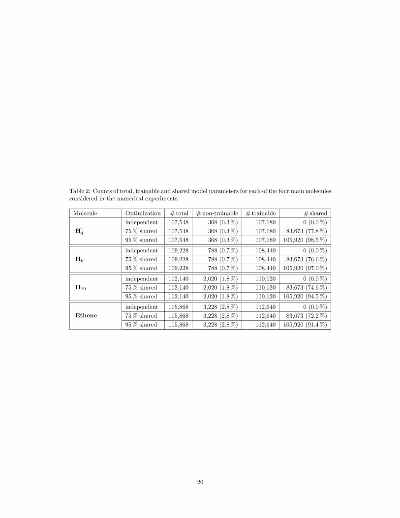
Table 2: Counts of total, trainable and shared model parameters for each of the four main moleculesconsidered in the numerical experiments.

Molecule Optimization # total # non-trainable # trainable # shared

H+4

independent 107,548 368 (0.3 %) 107,180 0 (0.0 %)

75 % shared 107,548 368 (0.3 %) 107,180 83,673 (77.8 %)

95 % shared 107,548 368 (0.3 %) 107,180 105,920 (98.5 %)

H6

independent 109,228 788 (0.7 %) 108,440 0 (0.0 %)

75 % shared 109,228 788 (0.7 %) 108,440 83,673 (76.6 %)

95 % shared 109,228 788 (0.7 %) 108,440 105,920 (97.0 %)

H10

independent 112,140 2,020 (1.8 %) 110,120 0 (0.0 %)

75 % shared 112,140 2,020 (1.8 %) 110,120 83,673 (74.6 %)

95 % shared 112,140 2,020 (1.8 %) 110,120 105,920 (94.5 %)

Ethene

independent 115,868 3,228 (2.8 %) 112,640 0 (0.0 %)

75 % shared 115,868 3,228 (2.8 %) 112,640 83,673 (72.2 %)

95 % shared 115,868 3,228 (2.8 %) 112,640 105,920 (91.4 %)

20

Supplementary information

S1 Weight-sharing and pre-training with ADAM

Figure S1 and Figure S2 show results for the experiments presented in the main text in Section 2.1and Section 2.2, respectively, when using the first-order ADAM [1] optimizer instead of second-order K-FAC optimization. The changed optimization hyperparameters are compiled in Table S1.

64 256 1,024 4,096 16,384

0

1

2

3

4

5

6

ener

gy re

l. to

MRC

I / m

Ha ~5x


Independent opt.75% of weights shared95% of weights sharedChem. acc.: 1 kcal/mol

64 256 1,024 4,096 16,384

0

1

2

3

4

5

6~10x

H6: 49 geometries


0

2

4

6

8

10

ener

gy re

l. to

MRC

I / m

Ha ~10x

H10: 49 geometries


0

5

10

15

20

25

30~9x

Ethene: 30 geometries

Optimizer: ADAM

Figure S1: Mean evaluation error relative to the reference calculation (MRCI-F12(Q)/cc-pVQZ-F12) as a function of training epochs per geometry for four different sets of nuclear geometries.Shadings indicate the area between the 25 % and the 75 % percentile of considered geometries. Foreach method, we plot intermediary and final results for optimizations that ran for a total numberof 16,384 epochs per geometry.

1

arX

iv:2

105.

0835

1v2

[ph

ysic

s.co

mp-

ph]

17

Dec

202

1

64 256 1,024 4,096 16,384

0

1

2

3

4

5

6en

ergy

rel.

to M

RCI /

mHa


Independent opt.(geom. of shared exp.)Pre-trained by shared opt.Chem. acc.: 1 kcal/mol

64 256 1,024 4,096 16,384

0

1

2

3

4

5

6H6: 23 geometries


0

2

4

6

8

10

ener

gy re

l. to

MRC

I / m

Ha

H10: 23 geometries


0

5

10

15

20

25

30Ethene: 20 geometries

Optimizer: ADAM

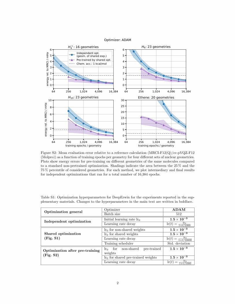
Figure S2: Mean evaluation error relative to a reference calculation (MRCI-F12(Q)/cc-pVQZ-F12(Molpro)) as a function of training epochs per geometry for four different sets of nuclear geometries.Plots show energy errors for pre-training on different geometries of the same molecules comparedto a standard non-pretrained optimization. Shadings indicate the area between the 25 % and the75 % percentile of considered geometries. For each method, we plot intermediary and final resultsfor independent optimizations that ran for a total number of 16,384 epochs.

Table S1: Optimization hyperparameters for DeepErwin for the experiments reported in the sup-plementary materials. Changes to the hyperparameters in the main text are written in boldface.

Optimization generalOptimizer ADAMBatch size 512

Independent optimizationInitial learning rate lr0 1.5× 10−3


Shared optimization(Fig. S1)

lr0 for non-shared weights 1.5× 10−3

lr0 for shared weights 1.5× 10−3


Training scheduler Std. deviation

Optimization after pre-training(Fig. S2)

lr0 for non-shared pre-trainedweights

1.5× 10−3

lr0 for shared pre-trained weights 1.5× 10−3


2

S2 Independent optimization as pre-training

In the main text, mere independent optimization was used as a benchmark for all numericalexperiments. Here, we consider an additional baseline, for which independent optimizations fordifferent ethene configurations were fully initialized with weights from a wavefunction that hadalready been optimized for a similar but different molecular configuration using an independentoptimization scheme. Optimization hyperparameters for the new benchmark are the same as theones reported in Table 1 in the main text. The respective results, including a comparison withshared optimization and independent optimzation that was pre-trained on a set of different etheneconfigurations using shared-weight constraints, are shown in Figure S3. While the new benchmarkseems to be advantageous during early optimization as compared to a scheme that applies aweight-sharing constraint for 95 % of the weights in the model, at the time the wavefunctions reachchemical accuracy, shared optimization without pre-training outperforms this new baseline to adegree comparable with the results shown in Figure 2 in the main text.


0

5

10

15

20

ener

gy re

l. to

MRC

I / m

Ha

Twisted and stretched EtheneIndependent opt.Full-weight-reuse from indep. opt.Reuse from 95%-shared opt.Shared opt. (95% shared)Chem. acc.: 1 kcal/mol

Figure S3: Mean evaluation error relative to the reference calculation (MRCI-F12(Q)/cc-pVQZ-F12) as a function of training epochs per geometry for a set of differently twisted and stretechedethene configurations. Shadings indicate the area between the 25 % and the 75 % percentile ofconsidered geometries. For each method, we plot intermediary and final results for optimizationsthat ran for a total number of 16,384, respectively 8,192, epochs per geometry.

References

1. Kingma, D. P. & Ba, J. Adam: A Method for Stochastic Optimization 2017. arXiv: 1412.6980[cs.LG].

3

nuclear geometries with weight-sharing deep neural networks

Documents