nuclear fission in monte carlo particle transport...
TRANSCRIPT

LA-UR-14-26868 - 1!
!!!
Nuclear Fission in!Monte Carlo Particle!
Transport Simulations!!
Forrest Brown!!
Senior Scientist!Monte Carlo Codes Group, XCP-3!Los Alamos National Laboratory!
FIESTA 2014 !Fission School & Workshop!Santa Fe, NM, Sept 8-12, 2014!

LA-UR-14-26868 - 2!
Abstract!
!Nuclear Fission in Monte Carlo Particle Transport Simulations!
!
Forrest B. Brown, XCP-3, LANL!!!Monte Carlo computer codes have been used to simulate neutron transport in fissionable materials since the late 1940s. Today’s MC codes such as MCNP6 can accurately model nearly any geometry and make use of detailed physics interaction data from the ENDF/B- VII libraries. For many applications today, many billions of neutrons are simulated using MC methods on parallel computers. While MC methods for neutron transport can be viewed in practical terms (i.e., just simulate particle behavior), there is a solid mathematical and physical basis founded in the linear Boltzmann transport equation. This lecture provides an overview of MC methods for simulating particle transport, with particular emphasis on the fundamental assumptions in the underlying equations and transport and collision modeling. Depending on the application, some portions of the simulations may use expected-value outcomes, while other portions require detailed modeling that conserves energy, momentum, particles, correlations, etc. Static eigenvalue calculations are compared with fixed-source time dependent approaches, and the detailed modeling of fission processes in MCNP is reviewed. !

LA-UR-14-26868 - 3!
Outline!
• Introduction!!
• Monte Carlo simulation and the transport equation!– Overview, particle simulation, theory, assumptions!– Eigenvalue problems vs. fixed-source time dependent problems !
!
• Using expected-value outcomes vs. detailed modeling!– Analog vs weighted simulation!– Transport process and Doppler broadening!– Collision physics and particle production!
!
• Fission process modeling in MCNP!– Expected-value approach for eigenvalue calculations!– Detailed modeling of multiplicity and correlated particle production!– Spontaneous vs. induced fission!– Emission spectra !

LA-UR-14-26868 - 4!
Introduction!
LA-UR-14-26868 - 5!
Monte Carlo & MCNP History!
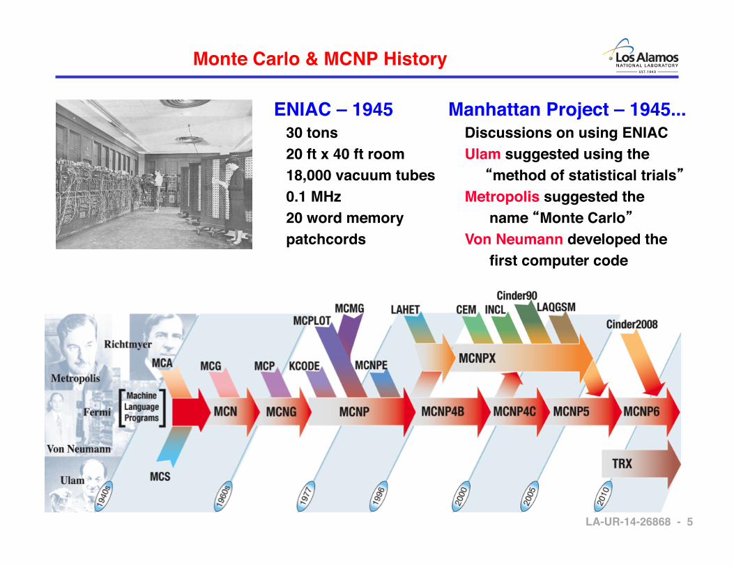
ENIAC – 1945! 30 tons! 20 ft x 40 ft room! 18,000 vacuum tubes! 0.1 MHz ! 20 word memory! patchcords!
Manhattan Project – 1945...! Discussions on using ENIAC! Ulam suggested using the! �method of statistical trials�! Metropolis suggested the! name �Monte Carlo�! Von Neumann developed the ! first computer code!

LA-UR-14-26868 - 6!
MCNP6 Features !
mcnp6! mcnpx!33 other particle types!
heavy ions!CINDER depletion/burnup!
delayed particles!!
Partisn mesh geometry!Abaqus unstructured mesh!
mcnp5 – 100 K lines of code!mcnp6 – 500 K lines of code!
High energy physics models!CEM, LAQGSM, LAHET!
MARS, HETC !
New Criticality Features!Sensitivity/Uncertainty Analysis!
Fission Matrix!OTF Doppler Broadening!
Continuous Testing System!~10,000 test problems / day!
mcnp6!protons, proton radiography!high energy physics models!
magnetic fields!
mcnp5!neutrons, photons, electrons!cross-section library physics!
criticality features!shielding, dose!
“low energy” physics!V&V history!
documentation!
Fission!MCNP5/X multiplicity!LLNL fission package!
CGM/LLNLGAM, CGMF (soon)!

LA-UR-14-26868 - 7!
MCNP & Nuclear Criticality Safety (1)!
Zeus-2, HEU-MET-INTER-006, case 2!
HEU-MET-THERM-003! PU-MET-FAST-003, case 3!
IEU-COMP-THERM-002, case 3! PNL-33 - MIX-COMP-THERM-002!

LA-UR-14-26868 - 8!
MCNP & Nuclear Criticality Safety (2)!

LA-UR-14-26868 - 9!
MCNP & Reactors (1) - PWR Analysis!
Whole-core Thermal & Total Flux from MCNP5 Analysis!
Assembly Thermal & Fast Flux from MCNP5 Analysis!
(from Luka Snoj, Jozef Stefan Inst.)!

LA-UR-14-26868 - 10!
3D geometry!
MCNP & Reactors (2) - TRIGA Reactor LEU Conversion !
Fast Flux! Thermal Flux!
Diffusion!Theory!Codes!
MCNP!Analysis!
Radial Power Density!From MCNP Analysis! (from Luka Snoj, Jozef Stefan Inst.)!

LA-UR-14-26868 - 11!
Monte Carlo Simulation!&!
the Transport Equation !

LA-UR-14-26868 - 12!
Monte Carlo - Introduction!
• Goal: !Simulate nature, ! ! ! !particles moving through physical objects!!
!Flight!!Random sampling using ΣT & exponential PDF:!• Free-flight distance! to next collision, s!!Ray-tracing in 3D computational geometry!
Collision!!Random sampling using !nuclear data:!• Collision isotope!• Reaction type!• Exit E' & Ω'!• Secondary particles!• Absorb or reduce weight!
During analysis of both flights & collisions,! tally information about distances, collisions, etc.! to use later in statistical analysis for results"

LA-UR-14-26868 - 13!
Monte Carlo Calculations!
• After a particle emerges from source or collision, or if the particle is entering a new cell:!
– Randomly sample the free-flight distance to the next interaction!
– If distance-to-interaction < distance-to-boundary, then move the particle to the interaction point!
– Collision physics at the interaction point:!• Determine which isotope the interaction is with!• Determine which reaction type for that isotope!• Determine the exit energy & direction of the particle!• Determine if secondary particles were produced!• Biasing + weight adjustments!• Tallies of quantities of interest!

LA-UR-14-26868 - 14!
Sampling the Flight Distance!
• Given a particle in a cell containing material M, sample the free-flight distance to the next interaction!
� ΣT = total macroscopic cross-section in material M!! = probability of any interaction per unit distance, units cm-1!
– PDF for flight distance s, where 0 ≤ s ≤ ∞,!!
! ! !f(s) = ΣT exp( -ΣT s )!
– Sampling procedure!!
! ! !F(s) = 1 - exp( -ΣT s ) � s = - ln(ξ) / ΣT !
ΣT (E) = N k ⋅σ Tk
k
nuclidesin material
∑ (E)

LA-UR-14-26868 - 15!
Selecting the Collision Isotope!
• ! ! !where k = isotopes in material M"
• Probability that collision is with isotope J!!!!
• { pJ } = set of discrete probabilities for selecting collision isotope!!• { PJ } = discrete CDF, !
• Discrete sampling for collision isotope k!! !table search to determine k such that Pk-1 ≤ ξ < Pk!
ΣT = NkσTk
k∑
pJ =NJσT
J
ΣT
PJ = pkk=1
J
∑

LA-UR-14-26868 - 16!
Selecting the Reaction Type!
• For collision isotope k,!
! !σT = σelastic + σinelastic + σcapture + σfission + …..!!• pJ = σJ / σT = probability of reaction type J for isotope k!
• { pJ } = set of discrete probabilities for selecting reaction type J!
• { PJ } = discrete CDF, !
• Discrete sampling for reaction type J!! !table search to determine J such that PJ-1 ≤ ξ < PJ!
PJ = pkk=1
J
∑

LA-UR-14-26868 - 17!
Sampling Exit Energy & Direction!
• Given a collision isotope k & reaction type j, the random sampling techniques used to determine the exit energy and direction, E' and (u',v',w'), depend on !– Conservation of energy & momentum!– Scattering laws - either equations or tabulated data!
• Examples !– Isotropic scattering in lab system !!– Elastic scattering, target-at-rest!– Elastic scattering, free-gas model !!– Inelastic scattering!– S(α,β) thermal scattering!– Other collision physics, MCNP!

LA-UR-14-26868 - 18!
Inelastic Scattering - MCNP!
Law 1 !- ENDF law 1 - Equiprobable energy bins!Law 2 !- Discrete photon energies!Law 3 !- ENDF law 3 - Inelastic scatter from nuclear levels!Law 4 !- ENDF law 4 - Tabular distribution!Law 5 !- ENDF law 5 - General evaporation spectrum!Law 7 !- ENDF law 7 - Simple Maxwell fission spectrum!Law 9 !- ENDF law 9 - Evaporation spectrum!Law 11 !- ENDF law 11 - Energy dependent Watt spectrum!Law 22 !- UK law 2 - Tabular linear functions of incident energy out!Law 24 !- UK law 6 - Equiprobable energy multipliers!Law 44 !- ENDF law 1, lang 2, Kalbach-87 correlated energy-angle scatter!Law 61 !- ENDF law 11, lang 0,12, or 14 - correlated energy-angle scatter!Law 66 !- ENDF law 6 - N-body phase space distribution!Law 67 !- ENDF law 7 - correlated energy-angle scatter!

LA-UR-14-26868 - 19!
Other Collision Physics - MCNP!
– Emission from fission!– Delayed neutron emission!– S(α,β) scattering for thermal neutrons!– Free-gas scattering for neutrons!– Probability tables for the unresolved resonance energy range!
– Photon interactions!• Photoelectric effect"• Pair production"• Compton scattering (incoherent)"• Thomson scattering (coherent)"• Fluorescent emission"• Photonuclear reactions"
– Electron interactions - condensed history approach!• Stopping power, straggling, angular deflections"• Bremsstrahlung"• K-shell impact ionization & Auger transitions"• Knock-on electrons"
LA-UR-14-26868 - 20!
Monte Carlo Simulation - Assumptions!
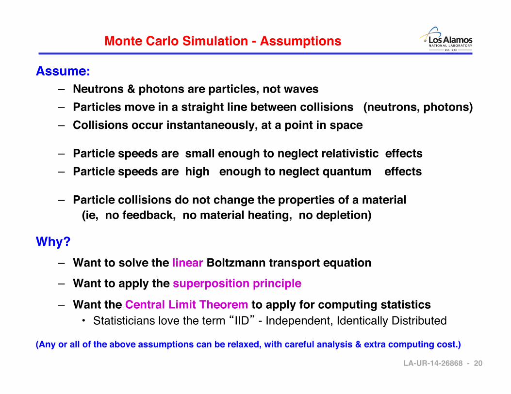
Assume:!– Neutrons & photons are particles, not waves!– Particles move in a straight line between collisions (neutrons, photons)!– Collisions occur instantaneously, at a point in space!
– Particle speeds are small enough to neglect relativistic effects!– Particle speeds are high enough to neglect quantum effects!
– Particle collisions do not change the properties of a material !(ie, no feedback, no material heating, no depletion)!
Why?!– Want to solve the linear Boltzmann transport equation!– Want to apply the superposition principle!– Want the Central Limit Theorem to apply for computing statistics!
• Statisticians love the term �IID� - Independent, Identically Distributed"!
(Any or all of the above assumptions can be relaxed, with careful analysis & extra computing cost.)!

LA-UR-14-26868 - 21!
• Time-dependent linear Boltzmann transport equation for neutrons, with prompt fission source & external source"
!!!!!!!
• This equation can be solved directly by Monte Carlo, assuming:"– Each neutron history is an IID trial (independent, identically distributed)!– All neutrons must see same probability densities in all of phase space!– Usual method: geometry & materials fixed over solution interval Δt!
Linear Boltzmann Transport Equation!
1v∂ψ(r,E,Ω,t)
∂t= Q(
r,E,Ω,t) + ψ(
r, ′E , ′
Ω ,t)ΣS(
r, ′E →E,
Ω⋅′Ω )∫∫ d′Ω d ′E
+ χ(r,E)4π
νΣF(r, ′E )ψ(∫∫
r, ′E , ′
Ω ,t)d
′Ω d ′E
−Ω⋅∇ + ΣT(
r,E)⎡⎣ ⎤⎦ ⋅ ψ(
r,E,Ω,t)
1v∂ψ(r,E,Ω,t)
∂t= Q + [S +M] ⋅ ψ − [L + T] ⋅ ψ
External source! Scattering!
Multiplication!
Leakage! Collisions!
Gains Losses

LA-UR-14-26868 - 22!
Monte Carlo & Transport Equation!
• Derive integral equation, in kernel form!– Start with integro-differential equation!– Use integrating factor!
– Define!!!
!!
!Collision density:!!!
!Transport kernel: !!!!
!Collision kernel:!!– Then!
exp − ΣT (!r − RΩ̂,E)d ′R
0
R
∫⎡
⎣⎢
⎤
⎦⎥, where RΩ̂ = !r − !′r
T ( ′!r → !r ,
!E) = ΣT (
!r ,E) ⋅exp − ΣT (!′r + sΩ̂,E)ds
0
!r−!′r
∫⎡
⎣⎢⎢
⎤
⎦⎥⎥⋅δ Ω̂i
!r−!′r!r−!′r −1( )!r−!′r 2
!E = E ⋅ Ω̂
Ψ(!r ,!E) = ΣT (
!r ,E) ⋅ψ (!r ,!E)
C(!′E →!E, !r ) = ΣS (
!r ,!′E →!E)
ΣT (!r , ′E )
+ χ(E)νΣF (!r , ′E )
4π ⋅ΣT (!r , ′E )
Ψ(!r ,
!E) = Ψ(!′r ,
!′E ) ⋅C(
!′E →!E, !′r )d
!′E + Q( ′!r ,
!′E )∫⎡⎣ ⎤⎦∫ ⋅T (!′r → !r ,
!E)d!′r
Reference: "D.C. Irving, "The Adjoint Boltzmann Equation and Its Simulation by Monte Carlo""" "Nuclear Engineering & Design 15, 273-292 (1971)"

LA-UR-14-26868 - 23!
Basis for the Monte Carlo Solution Method!!
Monte Carlo & Transport Equation!
Let p = (!r,!E) and R( ′p → p) = C(
!′E →!E,!′r ) ⋅T(!′r →
!r,!E)
Expand Ψ into components having 0,1,2,...,k collisions
Ψ(p) = Ψk(p)k=0
∞
∑ , with Ψ0(p) = Q(!′r ,!E) ⋅T(!′r →
!r,!E)d!′r∫
By definition,Ψk(p) = Ψk−1( ′p )∫ ⋅R( ′p → p)d ′p
Markovian: collision k depends only on the results of collision k-1,and not on any prior collisions k-2, k-3, ...
Ψ(!r ,
!E) = Ψ(!′r ,
!′E ) ⋅C(
!′E →!E, !′r )d
!′E + Q( ′!r ,
!′E )∫⎡⎣ ⎤⎦∫ ⋅T (!′r → !r ,
!E)d!′r

LA-UR-14-26868 - 24!
Histories!!
• After repeated substitution for Ψk !
!• A "history" is a sequence of states (p0, p1, p2, p3, …..)!
• For estimates in a given region, tally the occurrences for each collision of each "history" within a region!
Monte Carlo & Transport Equation!
Ψk(p) = Ψk−1( ′p )∫ ⋅R( ′p → p)d ′p
= ... Ψ0(p0 )∫ ⋅R(p0 → p1)∫ ⋅R(p1 → p2 )...R(pk−1 → p)dp0...dpk−1
p0
p1
p2 p3
p4 p1
p0 p2 p3
History 1!History 2"

LA-UR-14-26868 - 25!
!!!Monte Carlo approach:!!• Generate a sequence of states (p0, p1, p2, p3, …..) [i.e., a history]
by:!– Randomly sample from PDF for source: ! !Ψ0( p0 )!– Randomly sample from PDF for kth transition: !R( pk-1→pk )!
• Generate estimates of results by averaging over states for M histories:!
Monte Carlo & Transport Equation!
Ψk(p) = ... Ψ0(p0 )∫ ⋅R(p0 → p1)∫ ⋅R(p1 → p2 )...R(pk−1 → p)dp0...dpk−1
A = A(p) ⋅Ψ(p)dp∫ ≈ 1M
⋅ A(pk,m)k=1
∞
∑⎛⎝⎜⎞⎠⎟m=1
M
∑

LA-UR-14-26868 - 26!
• Random Walk for Particle!
• Particle History!
Particle Histories!
Track through geometry,"- select collision site randomly"- tallies"
Collision physics analysis,"- Select new E,Ω randomly"- tallies"
Secondary!Particles!
Source!- select r,E, Ω!
Random!Walk!
Random!Walk!
Random!Walk!
Random!Walk!
Random!Walk!
Random!Walk!

LA-UR-14-26868 - 27!
Fixed-source Monte Carlo Calculation!
!
Source!- select r,E, Ω!
Random!Walk! Random!
Walk!
Random!Walk!Random!
Walk!
Random!Walk!
Random!Walk!
Source!- select r,E, Ω!
Random!Walk! Random!
Walk!
Random!Walk!
Random!Walk!
Random!Walk!
Source!- select r,E, Ω!
Random!Walk! Random!
Walk!
Random!Walk!
Random!Walk!
Random!Walk!
Random!Walk!
History 1!
History 2!
History 3!

LA-UR-14-26868 - 28!
Keff Eigenvalue Equation !
• For problems with fission multiplication, another approach is to create a static eigenvalue problem from the time-dependent transport equation (the asymptotic or steady-state solution) !
• Introduce Keff, a scaling factor on the multiplication (ν)!
• Assume:!1. Fixed geometry & materials!2. No external source: !Q(r,E,Ω,t) = 0!3. ∂Ψ/∂t = 0:! ! !ν � ν / keff!
• Setting ∂Ψ/∂t = 0 and introducing the Keff eigenvalue gives!
!– Steady-state equation, a static eigenvalue problem for Keff and Ψk!– Keff = effective multiplication factor!– Keff and Ψk should never be used to model time-dependent problems.!
L + T[ ]Ψk(
r,E,Ω) = S+ 1
Keff
M⎡
⎣⎢
⎤
⎦⎥Ψk

LA-UR-14-26868 - 29!
Keff Eigenvalue Equation!
!!!!!!!!! ! ![ L + T ] !k != [S + 1/k M ] !k!
• The factor 1/k changes the relative level of the fission source, to balance the equation & permit a steady-state solution!
• Criticality!!Supercritical: !Keff > 1!
!Critical: ! !Keff = 1!
! Subcritical: !Keff < 1!
!Ω⋅∇ + ΣT(
!r,E)⎡⎣ ⎤⎦ ⋅ ψ(
!r,E,!Ω) = ψ(
!r, ′E , ′
!Ω )ΣS(
!r, ′E →E,
!Ω⋅!′Ω )∫∫ d!′Ω d ′E
+ 1keff
χ(E,!r )
4πνΣF(!r, ′E )ψ(∫∫
!r, ′E , ′
!Ω )d
!′Ω d ′E
Scattering!
Multiplication!
Leakage! Collisions!

LA-UR-14-26868 - 30!
Monte Carlo Eigenvalue calculation!
! Initial!Guess!
Cycle 1!Keff
(1)!Cycle 2!
Keff(2)!
Cycle 3!Keff
(3)!Cycle 4!
Keff(4)!
Cycle 1!Source!
Cycle 3!Source!
Cycle 4!Source!
Cycle 5!Source!
Cycle 2!Source!
Source!- select r,E, Ω!
Random!Walk! Random!
Walk!
Random!Walk!Random!
Walk!
Random!Walk!
Random!Walk!
Source!- select r,E, Ω!
Random!Walk! Random!
Walk!
Random!Walk!
Random!Walk!
Random!Walk!
Source!- select r,E, Ω!
Random!Walk! Random!
Walk!
Random!Walk!
Random!Walk!
Random!Walk!
Random!Walk!
Iterate (cycle) until converged, then more to accumulate tallies!

LA-UR-14-26868 - 31!
Using!Expected-value Outcomes!
vs!Detailed Modeling!

LA-UR-14-26868 - 32!
Analog vs Weighted Sumulations !
• Monte Carlo methods evaluate integrals using random sampling!– Random sampling introduces variance (noise) into the results!– More random sampling in the simulation � more variance!
• Statistical weights for particles can be used to permit replacing the random sampling of an event by the expected value for the event!
Scatter!
Absorb!Terminate!
Random selection of scatter vs absorb.!Estimate absorption for N collisions:!
S = 0"For k = 1 … N {"
"if ξ > σS/σT then S += 1"}"Absorption = S / N + statistical noise!
Always scatter, with reduced wgt.!Estimate absorption for N collisions:!
"
Absorption = [ N � (1- σS/σ T) ] / N = σS / σT!!
Replacing random sampling of an event by the expected value eliminates the variance contribution from the event. !
Analog Simulation!Scatter!
wgt’ = wgt � σS / σT!
Absorb! wgt’ = wgt · (1 – σS/σT )!
wgt = 1!
Weighted Simulation!

LA-UR-14-26868 - 33!
Typical Examples of Weighted Simulation!
• Doppler broadening!– For neutron flights through a material, we don’t randomly sample
target nuclide velocity for the ~ 1020 nuclides in the flight path!– We average the target nuclide cross-sections over a Maxwellian
distribution of nuclide velocities, and use the average cross-section to determine the flight distance!
• Criticality safety & reactor physics!– We routinely use “implicit capture”, where neutrons always survive a
collision with weight reduced by σS / σT!
– Some codes (not MCNP) model n-2n by scattering and multiply neutron weight by 2.!
– For neutrons produced by fission, routinely use expected value of wgt � ν "F / "T neutrons per collision!
– For photon production, routinely use wgt � σn�γ / σT photons produced per collision!
� Use of expected values implies uncorrelated outcomes!
LA-UR-14-26868 - 34!
Selecting the Reaction Type - Modified!
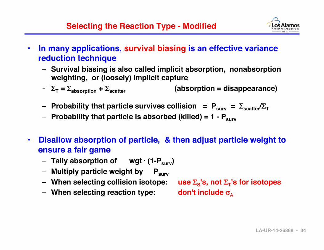
• In many applications, survival biasing is an effective variance reduction technique!– Survival biasing is also called implicit absorption, nonabsorption
weighting, or (loosely) implicit capture!� ΣT = Σabsorption + Σscatter ! !(absorption = disappearance)!
– Probability that particle survives collision = Psurv = Σscatter/ΣT !– Probability that particle is absorbed (killed) = 1 - Psurv!
• Disallow absorption of particle, & then adjust particle weight to ensure a fair game!– Tally absorption of wgt � (1-Psurv)!– Multiply particle weight by Psurv!– When selecting collision isotope: use ΣS's, not ΣT's for isotopes!– When selecting reaction type: don't include σ�-

LA-UR-14-26868 - 35!
Secondary Particle Creation!
• Consider a collision which results in fission! wgt • #ΣF / ΣT = !expected number of fission neutrons
! ! !produced per collision!
• To sample the number of neutrons produced in the collision!
– Let !r = wgt • #ΣF / ΣT!! !n = int[ r ]!
– Then, !Produce n fission neutrons with probability 1,! !and an additional fission neutron with probability r-n!
– Example:! wgt • #ΣF / ΣT = 1.75!!
! ! !If ξ < .75, produce 2 neutrons, otherwise produce 1!! ! or!! ! !Produce int[ 1.75 + ξ ] neutrons!

LA-UR-14-26868 - 36!
Fission Process!Modeling in MCNP6!

LA-UR-14-26868 - 37!
Background!
• Terrell!– probability for producing n fission neutrons!
"– Random sampling from a continuous Gaussian is easy!– Converting to integer is trivial, but does not preserve moments!– b = small adjustment, to preserve correct nu-bar!
– Traditional MCNP6 options differ only in schemes for sampling a Gaussian, converting to integer, & adjusting to preserve nu-bar!
• Measured data!– Terrell!– Zucker, Holden!– Gwin, Spencer, Ingle !
• Lestone method based on preserving moments!
LA-UR-05-0288
determined the relationships between the first threefactorial moments of the multiplicity distributions.
Table I. Neutron multiplicity distributions Pn for fast neutron induced fission of 235U [6]. Also given are themeasured mean multiplicities, [6], and the first three factorial moments of the given Pn.
P0 P1 P2 P3 P4 P5 P6 P7 1 2 3
2.55 0.0216 0.163 0.304 0.326 0.153 0.039 0.001 0.00 2.56 5.21 8.12.63 0.0190 0.140 0.307 0.316 0.164 0.043 0.002 0.00 2.59 5.40 8.72.68 0.0155 0.133 0.301 0.327 0.181 0.046 0.006 0.00 2.71 5.84 9.82.75 0.0136 0.118 0.299 0.326 0.194 0.053 0.007 0.00 2.78 6.15 10.62.81 0.0150 0.101 0.300 0.326 0.197 0.067 0.002 0.00 2.81 6.32 10.92.89 0.0100 0.091 0.290 0.312 0.233 0.053 0.017 0.00 2.91 6.82 12.73.04 0.0070 0.077 0.256 0.333 0.229 0.096 0.007 0.00 3.03 7.39 14.13.25 0.0050 0.060 0.202 0.335 0.264 0.111 0.028 0.00 3.25 8.64 18.43.42 0.0020 0.032 0.178 0.332 0.298 0.129 0.034 0.00 3.43 9.52 21.03.43 0.0024 0.041 0.174 0.329 0.278 0.140 0.037 0.00 3.41 9.57 21.53.54 0.0017 0.029 0.153 0.323 0.312 0.143 0.042 0.00 3.52 10.11 23.03.59 0.0014 0.018 0.164 0.292 0.333 0.154 0.040 0.00 3.56 10.36 23.83.67 -0.0004 0.024 0.133 0.307 0.323 0.159 0.054 0.00 3.62 10.78 25.63.74 0.0016 0.016 0.128 0.299 0.319 0.176 0.061 0.00 3.69 11.23 27.33.81 -0.0004 0.012 0.118 0.284 0.326 0.199 0.050 0.01 3.77 11.75 29.63.87 0.0001 0.007 0.113 0.278 0.332 0.197 0.073 0.00 3.82 12.01 30.23.88 -0.0002 0.012 0.104 0.270 0.324 0.218 0.054 0.02 3.88 12.54 33.23.97 0.0011 0.014 0.093 0.270 0.328 0.222 0.078 0.00 3.90 12.52 32.23.98 0.0009 0.007 0.086 0.267 0.332 0.184 0.112 0.01 3.97 13.22 36.24.09 0.0007 0.007 0.091 0.227 0.337 0.234 0.062 0.04 4.04 13.81 39.34.13 0.0001 0.008 0.070 0.243 0.312 0.260 0.071 0.04 4.13 14.35 41.54.21 0.0005 0.004 0.071 0.207 0.342 0.240 0.116 0.02 4.17 14.61 42.04.28 0.0001 0.002 0.066 0.206 0.343 0.250 0.104 0.03 4.21 14.86 43.24.35 0.0012 0.000 0.048 0.221 0.289 0.280 0.097 0.06 4.32 15.92 49.34.41 0.0000 0.003 0.044 0.186 0.280 0.377 0.018 0.10 4.46 16.84 53.64.49 0.0000 0.009 0.022 0.179 0.310 0.310 0.112 0.06 4.47 16.92 53.24.53 0.0000 0.003 0.048 0.146 0.338 0.248 0.193 0.03 4.50 17.04 53.3
III. MODELING NEUTRON MULTIPLICITYDISTRIBUTIONS
Measured neutron multiplicity distributions havebeen previously parameterized using Gaussiandistributions [8], and truncated renormalized singleand double Gaussians [9]. In the present paper therelationship between the first three factorial momentsis estimated assuming neutron multiplicitydistributions are Gaussian [8] and that the widths of these Gaussians are independent of incoming neutronenergy. By comparing the calculated relationshipbetween the factorial moments to the correspondingexperimental results [6] the validity of a fixed widthas a function of incoming neutron energy can betested.
Fig. 4 shows measured neutron multiplicitydistributions for thermal-neutron induced fission of
235U and 239Pu. Neutron multiplicity distributions canbe reasonably well represented by [8]
dxbxP 2/12
2
20 )2
)(exp(2
1 , and
dxbxP nnn
2/12/1 2
2
20 )2
)(exp(2
1 ,(1)
where is the mean multiplicity, b is a smalladjustment to make the mean equal to , and isthe root-mean-square width. To determined the valueof from experimental data many authors haveminimized the chi-squared
2
exp
exp2 )()(
n n
nn
PPP , (2)
2

LA-UR-14-26868 - 38!
MCNP6 – KCODE Calculations!
• For criticality calculations ! ![no external source, no spontaneous fission]!
– Neutron multiplicity for fission is based on expected value of wgt � ν "F
mat / "T
mat neutrons per collision in the material!Fmat
/ "Tmat neutrons per collision in the material!Tmat neutrons per collision in the material!
• If more than 1 neutron, the energy & direction for each are sampled independently (no correlation)"
– The spectrum used for the fission neutrons is randomly chosen using probabilities ν "F
iso / ν "T
mat for the nuclides in the material!Fiso
/ ν "Tmat for the nuclides in the material!Tmat for the nuclides in the material!
• Energy is sampled using ENDF spectrum data for the selected nuclide"• Prompt vs delayed neutron selected first, then energy "• If more than 1 neutron, energy is sampled independently for each one
(no correlation), using the same spectrum data"
– The direction for fission neutrons is sampled isotropically!• If more than 1 neutron, directions are sampled independently for each
neutron (no correlation in direction)"
– For KCODE problems with photons, photons are sampled independent of neutrons (no correlation between neutrons & photons)!

LA-UR-14-26868 - 39!
MCNP6 – KCODE Calculations!
• Why is the expected value approach to fission neutron production used for criticality calculations? Why not use explicit fission neutron multiplicity data?!
– Traditional MC work in the criticality safety community has focused on k-effective, reflector & control material reactivity, etc.!
– The reactor physics community has traditionally used MC for k-effective, power distributions, control material reactivity, etc.!
– Very extensive collections of verification-validation data, MC vs benchmark experiments for those applications!
� !No verification-validation work has been done to date !on using explicit fission neutron multiplicity options in !MCNP for criticality safety or reactor physics applications!

LA-UR-14-26868 - 40!
MCNP6 – Fixed-Source Calculations!
• For fixed-source problems, MCNP6 has a variety of options for treating fission neutron multiplicity !
• FMULT input card sets the option for each fissionable nuclide:!– Spontaneous fission:!
• Multiplicity: "nu-bar + Gaussian width or 10-bin distribution"• Spectrum: "Watt spectrum"
– Induced fission:!• MCNP traditional, based on expected value, ν "F
mat / "T
mat "Fmat
/ "Tmat "Tmat "
• Explicit multiplicity model options:"– Method"
» Lestone model (based on fits to moments)"» Ensslin/Santi/Beddingfield/Mayo model!» LLNL fission package (many options)"
– Data"» Terrell"» Lestone"» Ensslin/Santi/Beddingfield/Mayo !
– Shift"» Various options, preserves nu-bar
(needed when sampling integers from continuous distribution)"
LA-UR-14-26868 - 41!
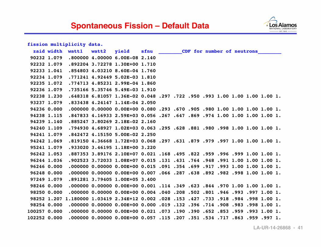
Spontaneous Fission – Default Data!
fission multiplicity data. zaid width watt1 watt2 yield sfnu ________CDF for number of neutrons________" 90232 1.079 .800000 4.00000 6.00E-08 2.140 " 92232 1.079 .892204 3.72278 1.30E+00 1.710 " 92233 1.041 .854803 4.03210 8.60E-04 1.760 " 92234 1.079 .771241 4.92449 5.02E-03 1.810 " 92235 1.072 .774713 4.85231 2.99E-04 1.860 " 92236 1.079 .735166 5.35746 5.49E-03 1.910 " 92238 1.230 .648318 6.81057 1.36E-02 0.048 .297 .722 .950 .993 1.00 1.00 1.00 1.00 1. " 93237 1.079 .833438 4.24147 1.14E-04 2.050 " 94236 0.000 .000000 0.00000 0.00E+00 0.080 .293 .670 .905 .980 1.00 1.00 1.00 1.00 1. " 94238 1.115 .847833 4.16933 2.59E+03 0.056 .267 .647 .869 .974 1.00 1.00 1.00 1.00 1. " 94239 1.140 .885247 3.80269 2.18E-02 2.160 " 94240 1.109 .794930 4.68927 1.02E+03 0.063 .295 .628 .881 .980 .998 1.00 1.00 1.00 1. " 94241 1.079 .842472 4.15150 5.00E-02 2.250 " 94242 1.069 .819150 4.36668 1.72E+03 0.068 .297 .631 .879 .979 .997 1.00 1.00 1.00 1. " 95241 1.079 .933020 3.46195 1.18E+00 3.220 " 96242 1.053 .887353 3.89176 2.10E+07 0.021 .168 .495 .822 .959 .996 .999 1.00 1.00 1. " 96244 1.036 .902523 3.72033 1.08E+07 0.015 .131 .431 .764 .948 .991 1.00 1.00 1.00 1. " 96246 0.000 .000000 0.00000 0.00E+00 0.015 .091 .354 .699 .917 .993 1.00 1.00 1.00 1. " 96248 0.000 .000000 0.00000 0.00E+00 0.007 .066 .287 .638 .892 .982 .998 1.00 1.00 1. " 97249 1.079 .891281 3.79405 1.00E+05 3.400 " 98246 0.000 .000000 0.00000 0.00E+00 0.001 .114 .349 .623 .844 .970 1.00 1.00 1.00 1. " 98250 0.000 .000000 0.00000 0.00E+00 0.004 .040 .208 .502 .801 .946 .993 .997 1.00 1. " 98252 1.207 1.180000 1.03419 2.34E+12 0.002 .028 .153 .427 .733 .918 .984 .998 1.00 1. " 98254 0.000 .000000 0.00000 0.00E+00 0.000 .019 .132 .396 .714 .908 .983 .998 1.00 1. "100257 0.000 .000000 0.00000 0.00E+00 0.021 .073 .190 .390 .652 .853 .959 .993 1.00 1. "102252 0.000 .000000 0.00000 0.00E+00 0.057 .115 .207 .351 .534 .717 .863 .959 .997 1. ""

LA-UR-14-26868 - 42!
MCNP6 – Induced Fission Neutron Multiplicity Options !
• Overly complicated – a result of recent merging of MCNP5 & MCNPX multiplicity treatments !
Comments from the MCNP6 routine acenus.F90:" ! Integer variable ifisnu determines the fission multiplicity " ! dataset for sampling the Gaussian width." ! ifisnu = abc" ! c = 1 Lestone data" ! c = 2 Terrell data" ! c = 3 Ensslin, Santi, Beddingfield, Mayo data" ! b = 0 MCNP5 shift to preserve nubar" ! b = 1 MCNPX shift to preserve nubar" ! b = 2 MCNPX threshold shift to preserve nubar" ! b = 3 MCNPX no shift to preserve nubar" ! b = 4 MCNPX nearest integer but with multiplicity prints" ! a = 0 MCNP5 normal_dist_sc Gaussian sampling" ! a >= 1 MCNPX normal_dist_po Gaussian sampling" ! a >= 2 MCNPX nu = nu + rang(), not MCNP5 nu = nu + half"
• Similar options & more also from LLNL Fission package in MCNP6!
LA-UR-14-26868 - 43!
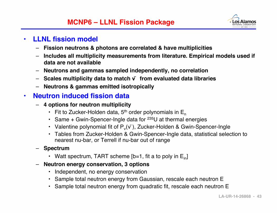
MCNP6 – LLNL Fission Package!
• LLNL fission model!– Fission neutrons & photons are correlated & have multiplicities!– Includes all multiplicity measurements from literature. Empirical models used if
data are not available!– Neutrons and gammas sampled independently, no correlation !– Scales multiplicity data to match ν ̄ from evaluated data libraries!– Neutrons & gammas emitted isotropically!
• Neutron induced fission data!– 4 options for neutron multiplicity!
• Fit to Zucker-Holden data, 5th order polynomials in En "• Same + Gwin-Spencer-Ingle data for 235U at thermal energies "• Valentine polynomial fit of Pν(ν ̄), Zucker-Holden & Gwin-Spencer-Ingle "• Tables from Zucker-Holden & Gwin-Spencer-Ingle data, statistical selection to
nearest nu-bar, or Terrell if nu-bar out of range"– Spectrum!
• Watt spectrum, TART scheme [b=1, fit a to poly in Ein]"– Neutron energy conservation, 3 options!
• Independent, no energy conservation"• Sample total neutron energy from Gaussian, rescale each neutron E"• Sample total neutron energy from quadratic fit, rescale each neutron E"

LA-UR-14-26868 - 44!
Random Sampling – Watt Spectrum!
Not widely known – !not used in MCNP!

LA-UR-14-26868 - 45!
MCNP6 – Work in Progress!
• For many years, patches to MCNP have existed for!
– Coincidence counting of fission neutrons!• Plan to incorporate the patches permanently into public version"
– Intrinsic sources – spontaneous fission!• Plan to incorporate the patches permanently into public version"
– List-mode data !• Can make use of exactly the same post-processing methods as for
experimental data"
• CGMF package will be added to MCNP6!
• Investigate use of multiplicity for MCNP criticality calculations (KCODE)!

LA-UR-14-26868 - 46!
References!
Monte Carlo References!700+ technical reports, presentations, etc., are available from the MCNP website – mcnp.lanl.gov,
under “Reference Collection”!Forrest Brown, “Fundamentals of Monte Carlo Particle Transport”, LA-UR-05-4983 (2005)"X-5 Monte Carlo Team, “MCNP - A General N-Particle Transport Code, Version 5” Volume I: Overview and Theory, LA-
UR-03-1987 (2003, updated 2005)"L.L. Carter and E.D. Cashwell, Particle Transport Simulation with the Monte Carlo Method, ERDA Critical Review Series,
TID-26607, National Technical Information Service, Springfield MA (1975).!Fission Neutrons & Physics!J. Terrell, “Distribution of Fission Neutron Numbers,” Phys. Rev., Vol. 108, No. 3, 783-789 (1957)."J. Terrell, “Fission Neutron Spectra and Nuclear Temperature”, Phys. Rev., Vol. 113, No. 2, 527-541 (1959"J.P. Lestone, “Energy and Isotope Dependence of Neutron Multiplicity Distributions”, Nucl. Sci. Eng. [also LA-UR-05-0288]"N. Ensslin, et al., “Application Guide to Neutron Multiplicity Counting”, LA-13422-M (1998)"J. Verbeke, C. Hagmann, D. M. Wright, “Simulation of Neutron and Gamma Ray Emission from Fission”, UCRL-AR-228518
(2007)"T. Wilcox, G.W. McKinney, T. Kawano, “MCNP6 Gets Correlated with CGM 3.4”, proceedings ANS RPSD 2014, LA-
UR-14-21300 (2014)."M. S. Zucker and N. Holden, “Parameters for Several Plutonium Nuclides and 252Cf of Safeguards Interest,” Proc. Sixth
Annual Symp. ESARDA, Venice, 1984, p. 341. "M. S. Zucker and N. Holden, “Energy Dependence of the Neutron Multiplicity Pν in Fast Neutron Induced Fission of
235,238U and 239Pu,” IAEA Conference on Nuclear Safeguards Technology, Vienna, November 1986, Vol. 2, p. 329. "R. Gwin, R.R. Spencer, R.W. Ingle, ”Measurements of the Energy Dependence of Prompt Neutron Emission from 233U,
235U, 239Pu, and 241Pu for En = 0.005 to 10 eV Relative to Emission from Spontaneous Fission of 252Cf,” Nucl. Sci. Eng., 87, 381 (1984). !
P. Santi, D.H. Beddingfield, D.R. Mayo, ”Revised prompt neutron emission multiplicity distributions for 236,238Pu,” Nucl. Phys. A 756, 325-332 (2005). "