The mathematics of diseases– On Modeling Hong Kong’s SARS Outbreak

Dr. Tuen Wai NgDepartment of Mathematics, HKU

Content

Basic Epidemic ModelingSIR ModelMy Recent works on Modeling of the SARS propagation in Hong Kong

Infectious disease modeling

Epidemics:

Black DeathEurope lost 1/3 of population in 1347 -

1350.Great Plague of London, 1664–66.

Killed more than 75,000 of total population of 460,000.

rat flea

Infectious disease modeling

Epidemics:

Influenza

killed 25 million in 1918-19 in Europe

influenza virus

Infectious disease modelingEpidemics:

AIDS

SARS

AIDS virus

Coronavirus

Infectious disease modelingEpidemics:

bovine spongiform encephalopathy(mad cow disease)

Chicken flu

Infectious disease modelingMathematical models can:

predict rate of spread, peak, etc., of epidemicspredict effects of different disease control strategies

.The WHO's eradication project

reduced smallpox (variola) deaths from two million in 1967 to zero in 1977–80.

Smallpox was officially declared eradicated in 1979. smallpox

virus

IndividualIndividual’’s s disease disease state :state : LatentLatent InfectiousInfectious

Immune / Immune / RemovedRemoved

timetimeEpoch :Epoch :

Serial interval

Incubation period

ttAA tBB tCC tDD tEE

Infection Infection occursoccurs

Latency to Latency to infectious infectious transitiontransition

Symptoms Symptoms appearappear

First First transmission transmission to another to another susceptiblesusceptible

Individual no Individual no longer longer

infectious to infectious to susceptiblessusceptibles(recovery or (recovery or

removal)removal)

Note : tD is constrained to lie in the interval (tB , tE), so tD > tC(as shown) and tD < tC are both possible.

SusceptibleSusceptible

Basic Assumptions of the simplest epidemic model, the SIR model

Population size is large and constant- No birth,death,immigration or emigration

No latencyHomogeneous mixing

- that is each pair of individuals has equal probability of coming into contact with one another (this is reasonable for a school or households in a building).

We divide the total population N into three groups:I) Susceptible class, St=S(t)=no. of susceptibles— those who may catch the disease but currently are not infected. II) Infective class, It=I(t)=no. of infectives— those who are infected with the disease and currently contagious. III) Removed class, Rt=R(t)=no. of removals— those who cannot get the disease, because they either have recovered permanently, are naturally immume, or have died.

Basic Assumptions of the SIR model

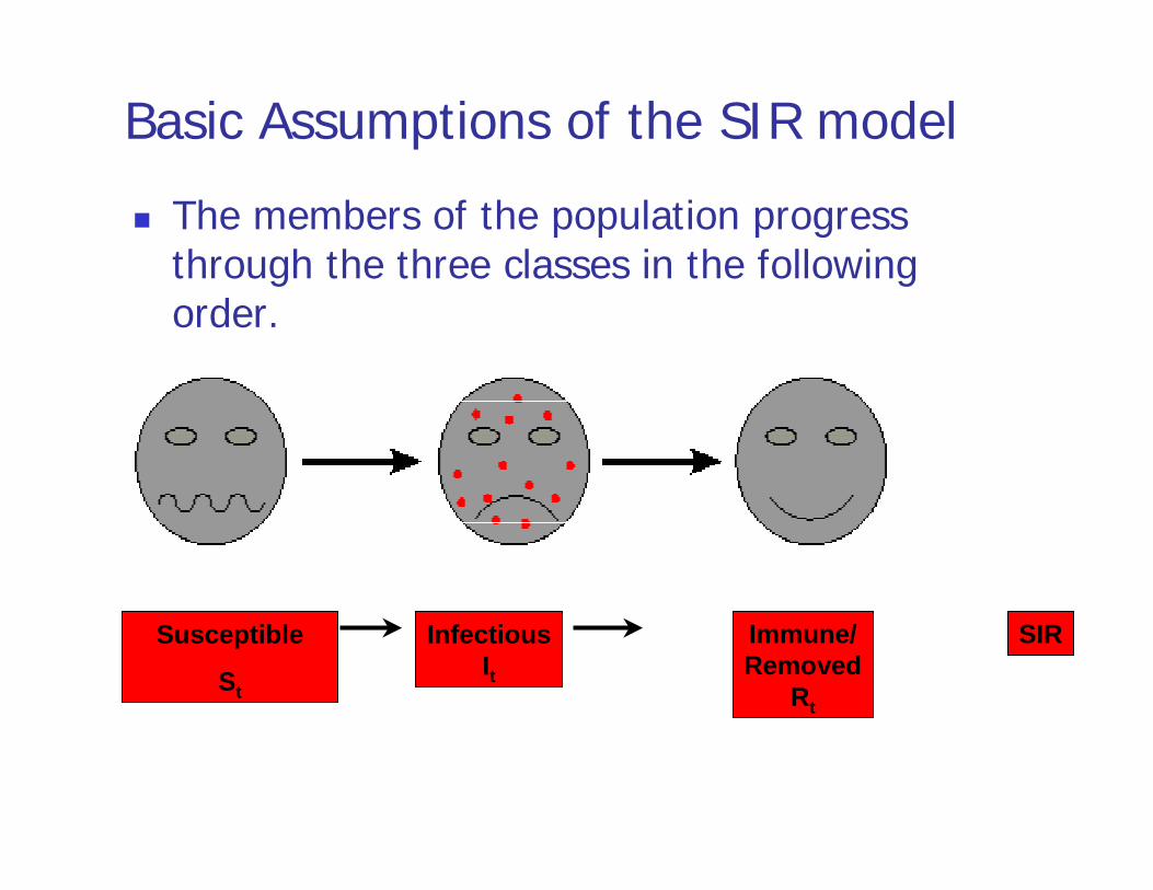
The members of the population progress through the three classes in the following order.

Basic Assumptions of the SIR model

Susceptible

St

InfectiousIt

Immune/Removed

Rt

SIR

Disease spreads when a susceptible individual comes in contact with an infected individual and subsequently becomes infected. Assuming homogeneous mixing, the mass action principle says that the number of encounters between susceptibles and infectivesis given by the product St It.However, only a proportion α of the contacts between susceptibles and infectives result in infection. Hence, in the next time interval,

Basic Assumptions of the SIR model

. 1 tttt ISSS α−=+

However, only a proportion α of the contacts between susceptibles and infectives result in infection. Hence, in the next time interval,

Basic Assumptions of the SIR model

. 1 tttt ISSS α−=+

Susceptible St

Infectious It

αStIt

During one time step, the infective class grows by the addition of the newly infected. At the same time, some infectives recover or die, and so progress to the removed stage of the disease.

The removal rate γ measures the proportion of the infective class that ceases to be infective, and thus moves into the removed class, in one step.

Basic Assumptions of the SIR model

Infectious It

Recovered / immune

Rt

γIt

Clearly the removed class increases in size by exactly the same amount that infected class decreases.

Therefore, we have

Basic Assumptions of the SIR model

,

ttt

ttttt

IRRIISII

γγα

+=−+=

+

+

1

1

Infectious It

Recovered / immune Rt

γItSusceptible St

αStIt

If we let ∆S= S t+1-St and similarly for ∆Iand ∆R, then the dynamics of the functions S,I and R are governed by the following equations.

. ,

- ,

ttt

ttttt

tttt

IRRRIISIII

ISSSS

γγα

α

=−=∆−=−=∆

=−=∆

+

+

+

1

1

1

For example, if I0 = 1, S0= 1000, R0=0, α =0.001and γ = 0.1, then S1=1000 - 0.001(1000)(1)=999

and I1= 1+ 0.001(1000)(1)-0.1(1) = 1.9 ~2.

Exercise 1: Find St,It and Rt when t =2.

Exercise 2: Use Excel to compute St,It and Rt for t from 0 to 100 and plot the graph of St,It and Rt .

0

100

200

300

400

500

600

0 4 8 12 16 20 24 28 32 36 40 44 48 52 56 60 64 68 72 76 80 84 88

I

S

R

Thread Values and Critical ParametersWe will say an epidemic occurs if ∆I >0 for some time t (i.e., if at some time t, the number of infectives grows).If ∆I < 0 for all times, then the size of the infective class does not increase and no wider outbreak of the disease takes place. Therefore, it is important to know when

)

tt

ttt

ISIISI

γαγα

−=−=∆

(

is positive, zero, or negative.

Let’s find out when ∆ I is zero.

) ttttt ISIISI γαγα −=−=∆ (

∆I =0 once It=0 (as the population is disease free). Now assume It >0, then we have

. 0 then , If

. 0 then , If

. 0 then , If

<∆<

=∆=

>∆>

IS

IS

IS

t

t

t

αγαγαγ

Note that St is a non-increasing function in t. Therefore, if , then for all t, .

αγ

<tS αγ

<0S

Thus, if S0 is below the value , then ∆ I< 0 for all times, and the disease decreases in the population. However, when , the number of infective will grow and an epidemic occurs. In other words, we have an outbreak if and only if

αγ

αγ>0S

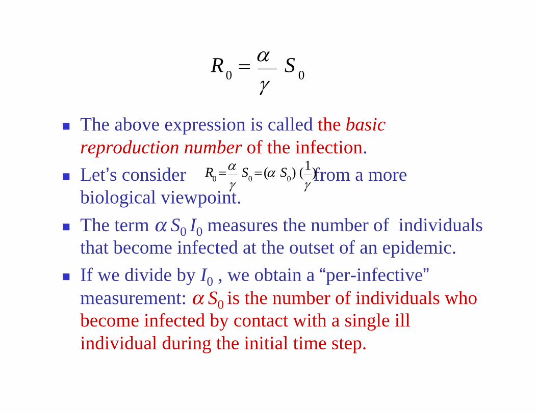
100 >= SR γα

00 SR γα=

The above expression is called the basic reproduction number of the infection. Let’s consider from a more biological viewpoint.The term α S0 I0 measures the number of individuals that become infected at the outset of an epidemic. If we divide by I0 , we obtain a “per-infective”measurement: α S0 is the number of individuals who become infected by contact with a single ill individual during the initial time step.

)1()( 000 γα

γα SSR ==

Actually, if we introduce one infective into a wholly susceptible population S0 , this ill individual may eventually infect many more than α S0 others, because an infective may remain contagious for many time steps. For example, suppose a young child remains contagious with chickenpox for about 7 days. Then, using a time step of 1 day, this child would infect about (α S0 ) (7)susceptibles over the course of a week. Moreover, if the period of contagion lasts 7 days, then each day we expect roughly or approximately 14% of the total number of infectives to move from the infective class It into the removed class Rt .

Because the removal rate γ measures the fraction of the infective class “cured” during a single time step, we have found a good estimate for γ ; we take

At the same time, we have found a good interpretation for 1/ γ : it is the average duration of infective class It into the removed class Rt .In fact, we can estimate γ for real diseases by observing infected individuals and determining the mean infectious period 1/ γ first.

1429.071≈=γ

In summary, we have

.

infection ofduration average

unit timeper infective

one from arising cases new of no.

1 ) ( 00

⎟⎟⎠

⎞⎜⎜⎝

⎛⎟⎟⎠

⎞⎜⎜⎝

⎛=

⎟⎟⎠

⎞⎜⎜⎝

⎛=

γα SR

Thus, R0 is interpreted as the average number ofsecondary infections that would be produced by an infective in a wholly susceptible population of size S0 .

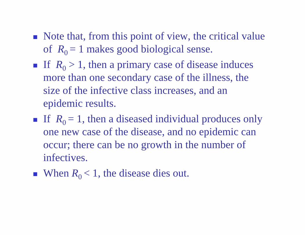
Note that, from this point of view, the critical value of R0 = 1 makes good biological sense. If R0 > 1, then a primary case of disease induces more than one secondary case of the illness, the size of the infective class increases, and an epidemic results. If R0 = 1, then a diseased individual produces only one new case of the disease, and no epidemic can occur; there can be no growth in the number ofinfectives.When R0 < 1, the disease dies out.

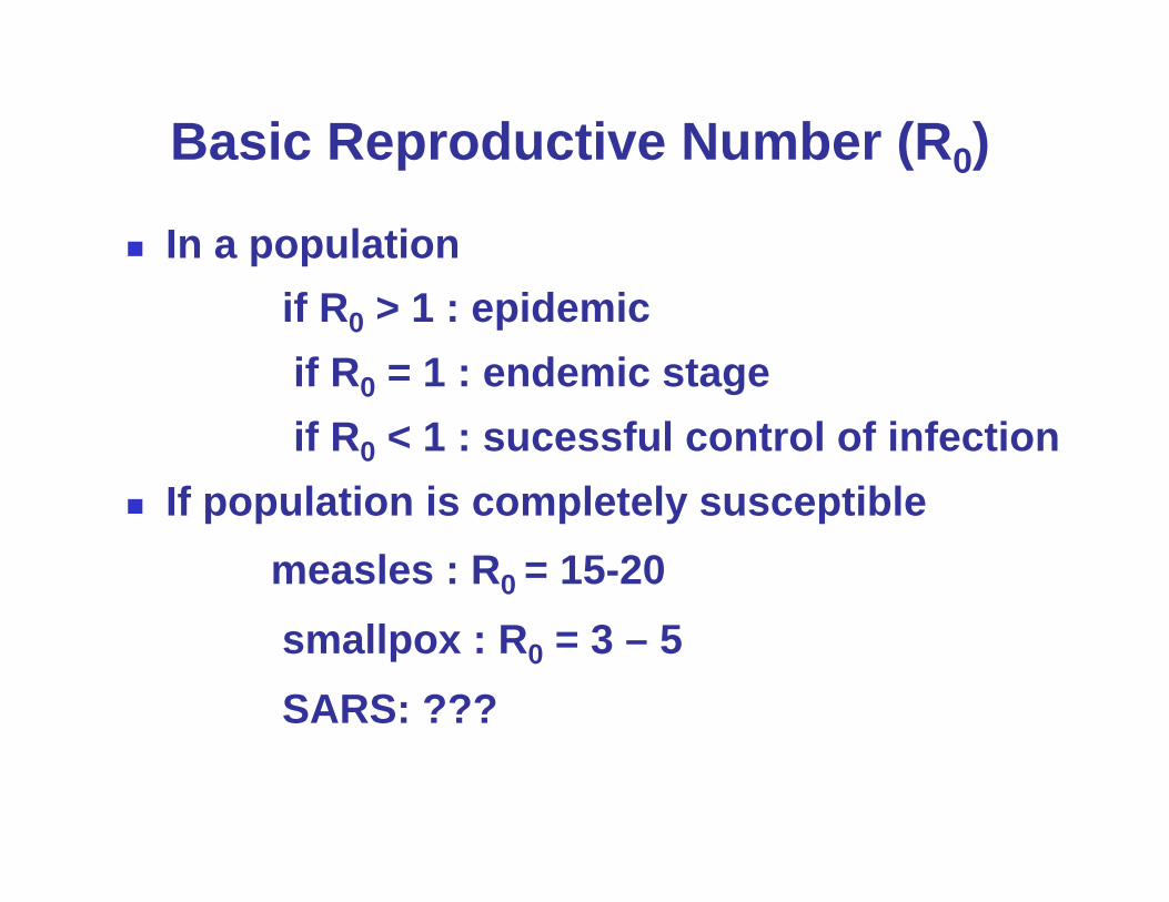
Basic Reproductive Number (R0)

In a populationif R0 > 1 : epidemicif R0 = 1 : endemic stageif R0 < 1 : sucessful control of infection

If population is completely susceptible measles : R0 = 15-20smallpox : R0 = 3 – 5SARS: ???

Continuous model

Note that so far we are using discrete time intervals (e.g. one day). Now if we let the time interval to be very small, say one second. Then ∆I is almost equal to the instinct change of I. Therefore, one may replace ∆I by dI/dt, which is the rate of change of I (also called the derivative of I). Similarly, we may replace ∆S and ∆R by dS/dt and dR/dt respectively. With these notations, our system of equations can be replaced by the following system of ordinary differential equations.

A system of three ordinary differential equations describes the SIR model:

)(

)()()(

)()(

tIdtdR

tItStIdtdI

tStIdtdS

γ

γα

α

=

−=

−=

where is α the infection rate and γ the removal rate of infectives.

Given such a system of differential equations, one would like to solve it (i.e. find functions S,I and R which satisfy the equations).In general, this system of differential

equations does not have any closed form solution. However, for given α and γ, we can solve the systems of differential equations by using some mathematical software like Mathlab. In general, the graphs of the S,I,R have the following shapes.

Graphs of S,I,R functions

Figure 1: Typical dynamics for the SIR model.

To learn more about differential calculus, you may take the following courses. MATH0801-Basic Mathematics I MATH0802-Basic Mathematics II MATH0803-Basic Mathematics III

To learn more about differential equations, you may take MATH2405-Differential Equations

To know more about how mathematics can be applied in biology, you may take MATH0011-Numbers and Patterns in Nature and Life.

Advertisement

Case study: The Hong Kong’s SARS Outbreak in 2003Since November 2002 (and perhaps earlier) an outbreak of a very contagious atypical pneumonia(now named Severe Acute Respiratory Syndrome,SARS) initiated in the GuangdongProvince of China. This outbreak started a world-wide epidemic after a medical doctor from Guangzhou infected several persons at a hotel in Hong Kong around February 21st, 2003.At the very beginning of SARS outbreak, SARS was believed to be a disease transmitted by respiratory droplets through close person-to-person contact.

Respiratory droplets are relatively large-sized particles and thus cannot travel long distances through air and therefore this mode of transmission cannot account for the rapid and wide spread of disease at Amoy Gardens, a housing estate in the Kowloon district of Hong Kong.

At that time, one may therefore ask if the modeof transmission is airborne.

It is well-known that influenza is an airborne disease.In the 4th March 1978 issue of the British

medical Journal, there was a report with detailed statistics of a flu epidemic in a boys boarding school with a total of 763 boys Of these 512 were confined to bed during the epidemic, which lasted from 22nd January to 4th February 1978. It seems that one infected boy initiated the epidemic. The SIR model was applied by J.D. Murray, to study the spread the flu epidemic in this school and he found that α= 0.00218 and γ= 0.440 and hence R0=3.78.

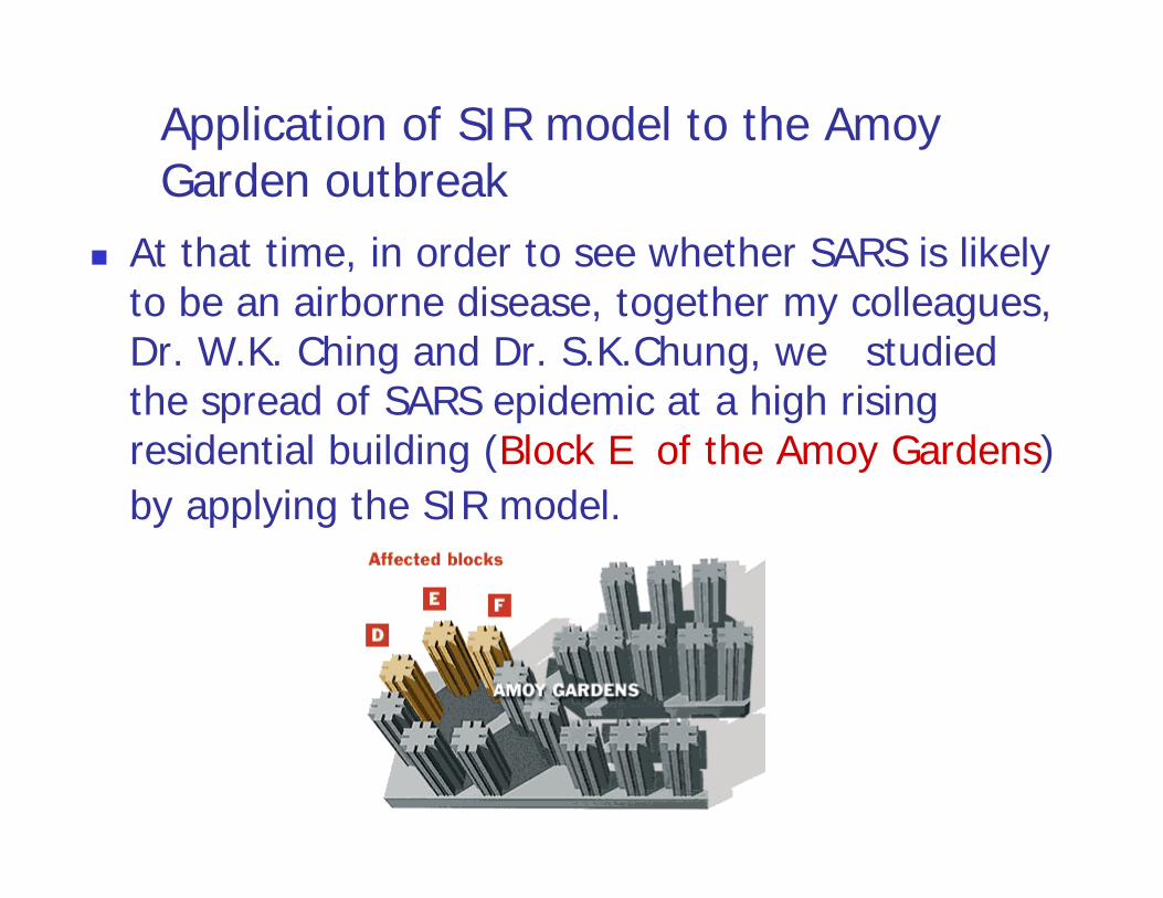
Application of SIR model to the Amoy Garden outbreak

At that time, in order to see whether SARS is likely to be an airborne disease, together my colleagues, Dr. W.K. Ching and Dr. S.K.Chung, we studied the spread of SARS epidemic at a high rising residential building (Block E of the Amoy Gardens) by applying the SIR model.

Since from 26th March 2003 to 30th March 2003, most of these confirmed cases are from Block E of the Amoy Gardens, we shall assume all of them are actually from Block E.

There are 33 floors, 8 flats each floor in Block E. Hence there are about 792 residents living in the building (we assume here that there are 3 people living in each flat and there are totally 8 ×33=264 flats in Block E). Therefore, we set S(0)= 792 - I(0).I(0) is unknown at that time.

It is believed that one infected resident (a super spreader) initiated the epidemic when he visited and stayed with his brother's family, so we assume that 0 < I(0) ≤ 4.Note that the infected number of residents I(t) at time t is unobservable (why?) and we assume R(t) is equal to the cumulative number of residents in Block E confirmed with SARS symptoms at time t.

Day 26/3/03 27/3/03 28/3/03 29/3/03 30/3/03

Confirmed Cases 7 22 56 78 112

PredictedCases 13 27 47 77 117

These numbers of confirmed cases and predicted cases (by the SIR model) are then summarized in the

table below.

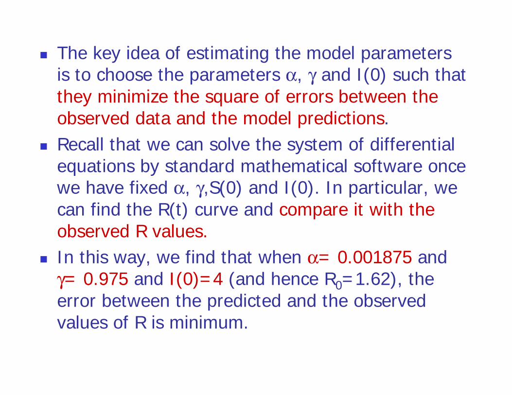
The key idea of estimating the model parameters is to choose the parameters α, γ and I(0) such that they minimize the square of errors between the observed data and the model predictions.Recall that we can solve the system of differential equations by standard mathematical software once we have fixed α, γ,S(0) and I(0). In particular, we can find the R(t) curve and compare it with the observed R values.In this way, we find that when α= 0.001875 and γ= 0.975 and I(0)=4 (and hence R0=1.62), the error between the predicted and the observed values of R is minimum.

For SARS, in the Block E of Amoy Gardens scenario, we found α= 0.001875 and γ= 0.975.For influenza, in the broadening school scenario, Murray found α= 0.00218 and γ= 0.44.We note that the value of the infection parameter α in this case is very closed to that of SARS at the Amoy Gardens. This suggests that both epidemics may have similar ways of transmission. At that time, a report of this finding was sent to the WHO.

The mystery of Amoy Gadrens remains unsolved even though there are several completing theories. Therefore, the mode of transmission is still not very clear. SARS appears to be transmitted mainly by person-to-person contact. However, it could also be transmitted by contaminated objects, air, or by other unknown ways. See the recent book “At the Epicentre”, published by Hong Kong University Press.

The pattern of the SARS outbreak in Hong Kong was puzzling after a residential estate (Amoy Gardens) in Hong Kong was affected, with a huge number of patients infected by the virus causing SARS. In particular it appeared that underlying this highly focused outbreak there remained a more or less constant background infectionlevel. This pattern is difficult to explained by the standard SIR epidemic model.

Another puzzle

This pattern is difficult to explain with the standard SIR model. Try to build another model.

0

10

20

30

40

50

60

70

80

90

03/1

7

03/2

0

03/2

3

03/2

6

03/2

9

04/0

1

04/0

4

04/0

7

04/1

0

04/1

3

04/1

6

04/1

9

04/2

2

04/2

5

04/2

8

05/0

1

05/0

4

05/0

7

05/1

0

Num

ber o

f cas

es

Hosiptal staffAmoy GardensCommunity

Figure 2: Daily new number of confirmed SARS cases from Hong Kong: hospital, community and the Amoy Gardens.

Joint Work WithGabriel TuriniciINRIA, Domaine de Voluceau,Rocquencourt, FranceAntoine DanchinGénétique des Génomes Bactériens,Institut Pasteur, Paris, France(Former director of HKU-Pasteur Institute)

A Double Epidemic Model for the SARS Propagation

Published in BMC Infectious Diseases2003, 3:19 (10 September 2003)

Can be found online at: http://www.biomedcentral.com/1471-2334/3/19

There are two epidemics, one is SARS caused by a coronavirus virus, call it virus A. Another epidemic, which may have appeared before SARS, is assumed to be extremely contagious because of the nature of the virus and of its relative innocuousness, could be propagated by contaminated food and soiled surfaces. It could be caused by somecoronavirus, call it virus B. The most likely is that it would cause gastro-enteritis.

Hypothesis of the Double Epidemic Model for the SARS Propagation

The most likely origin of virus A is a more or less complicated mutation or recombination event from virus B.Both epidemics would spread in parallel, and it can be expected that the epidemic caused by virus B which is rather innocuous, protects against SARS (so that naïve regions, not protected by the epidemic B can get SARS large outbreaks).

Hypothesis of the Double Epidemic Model for the SARS Propagation

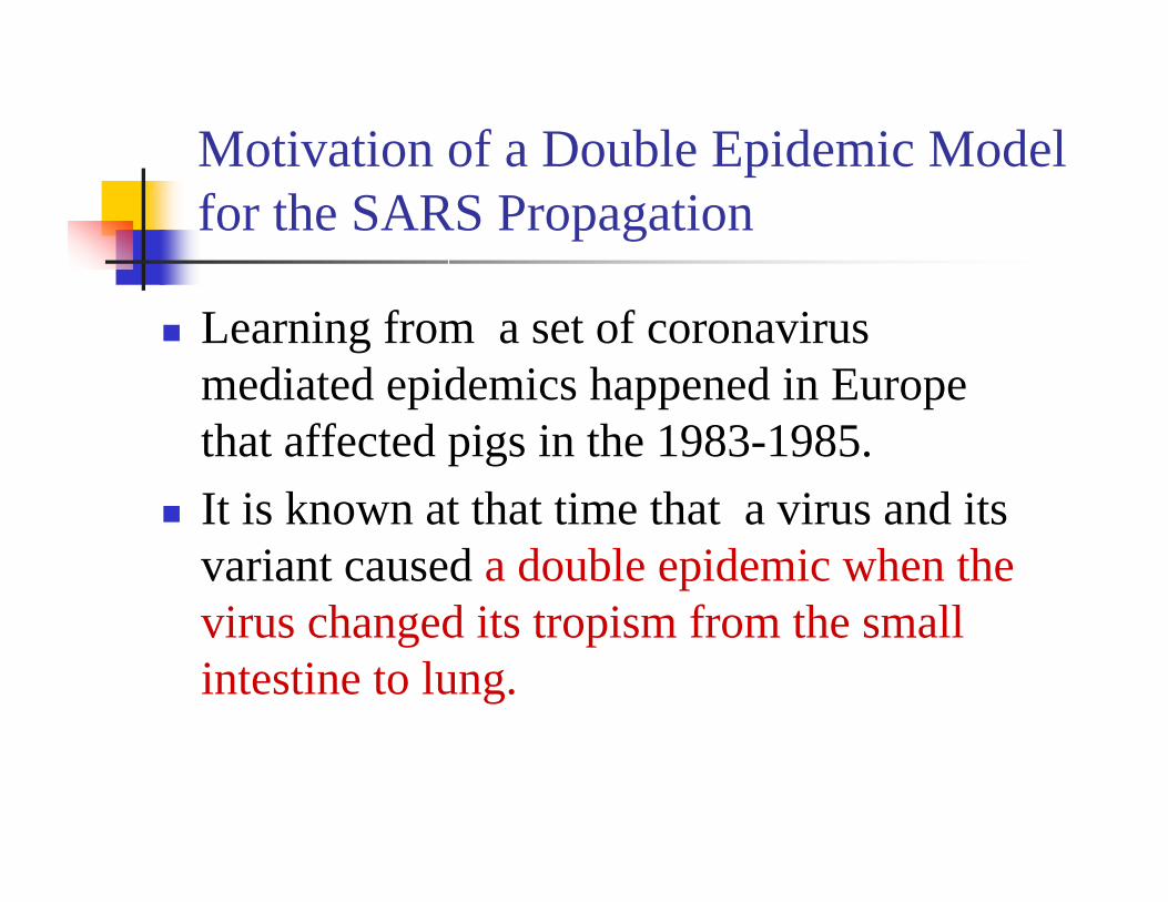
Learning from a set of coronavirusmediated epidemics happened in Europe that affected pigs in the 1983-1985.It is known at that time that a virus and its variant caused a double epidemic when the virus changed its tropism from the small intestine to lung.

Motivation of a Double Epidemic Model for the SARS Propagation

This in a way allowing the first one to provide some protection to part of the exposed population.D Rasschaert, M Duarte, H Laude: Porcine respiratory coronavirus differs from transmissible gastroenteritis virus by a fewgenomic deletions. J Gen Virol 1990, 71 ( Pt 11):2599-607.

Motivation of a Double Epidemic Model for the SARS Propagation

The hypothesis is based on:A) the high mutation and recombination

rate of coronaviruses.

SR Compton, SW Barthold, AL Smith: The cellular and molecular pathogenesis ofcoronaviruses. Lab Anim Sci 1993, 43:15-28.

A Double Epidemic Model for the SARS Propagation

B) the observation that tissue tropism can be changed by simple mutations .

BJ Haijema, H Volders, PJ Rottier: Switching species tropism: an effective way to manipulate the feline coronavirusgenome. J Virol 2003, 77:4528-38.

A Double Epidemic Model for the SARS Propagation

Assume that two groups of infected individuals are introduced into a large population. One group is infected by virus A.The other group is infected by virus B.Assume both diseases which, after recovery, confers immunity (which includes deaths: dead individuals are still counted). Assumed that catching disease B first will protect the individual from disease A.

A Double Epidemic SEIRP Model

We divide the population into six groups:— Susceptible individuals, S(t)— Exposed individuals for virus A, E(t) — Infective individuals for virus A, I(t)— Recovered individuals for virus A, R(t)— Infective individuals for virus B, Ip(t)— Recovered individuals for virus B, Rp(t)

A Double Epidemic SEIRP Model

The progress of individuals is schematically described by the following diagram.

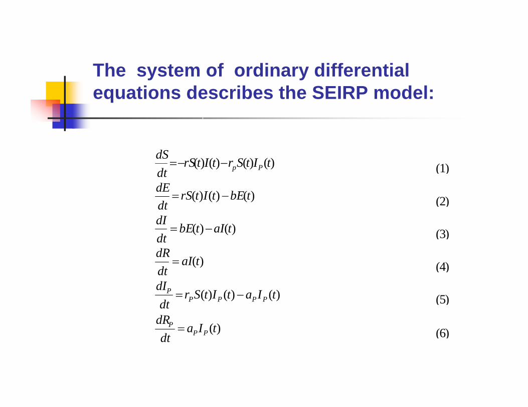
The system of ordinary differential equations describes the SEIRP model:

)()()()( tItSrtItrSdtdS

Pp−−= (1)

)()()( tbEtItrSdtdE

−= (2)

)()( taItbEdtdI

−= (3)

)(taIdtdR

= (4)

)()()( tIatItSrdt

dIPPPP

P −= (5)

)(tIadt

dRPP

P = (6)

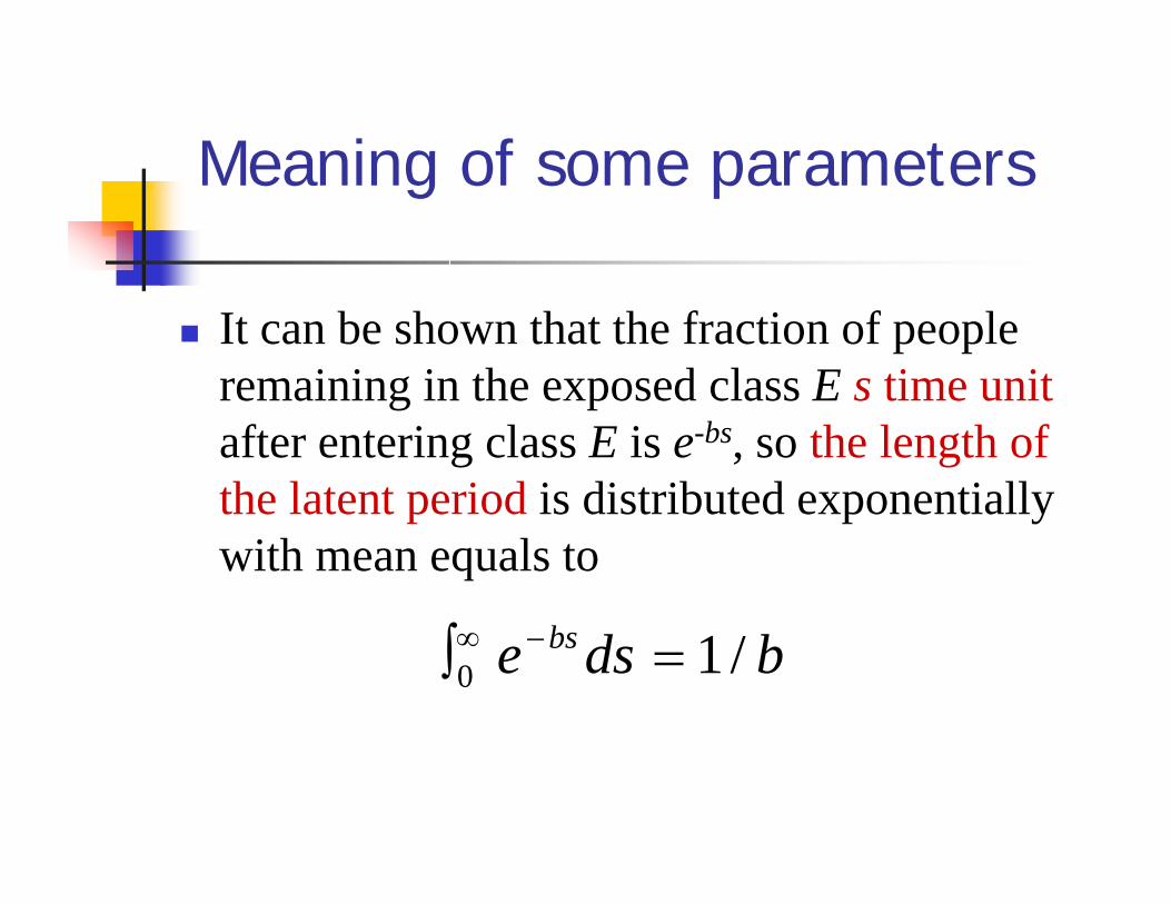
Meaning of some parameters

It can be shown that the fraction of people remaining in the exposed class E s time unitafter entering class E is e-bs, so the length of the latent period is distributed exponentially with mean equals to

bdse bs /10 =∫ −∞

Meaning of some parameters

It can be shown that the fraction of people remaining in the infective class I s time unitafter entering class I is e-as, so the length of the infectious period is distributed exponentially with mean equals to

adse as /10 =∫ −∞

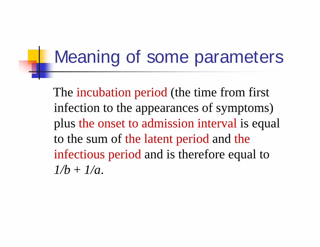
Meaning of some parameters

The incubation period (the time from first infection to the appearances of symptoms) plus the onset to admission interval is equal to the sum of the latent period and theinfectious period and is therefore equal to 1/b + 1/a.

Empirical Statistics

CA Donnelly, et al., Epidemiological determinants of spread of causal agent of severe acute respiratory syndrome in Hong Kong, The Lancet, 2003.The observed mean of the incubation period for SARS is 6.37.The observed mean of the time from onset to admission is about 3.75.Therefore, the estimated 1/a + 1/b has to be close to 6.37+3.75=10.12.

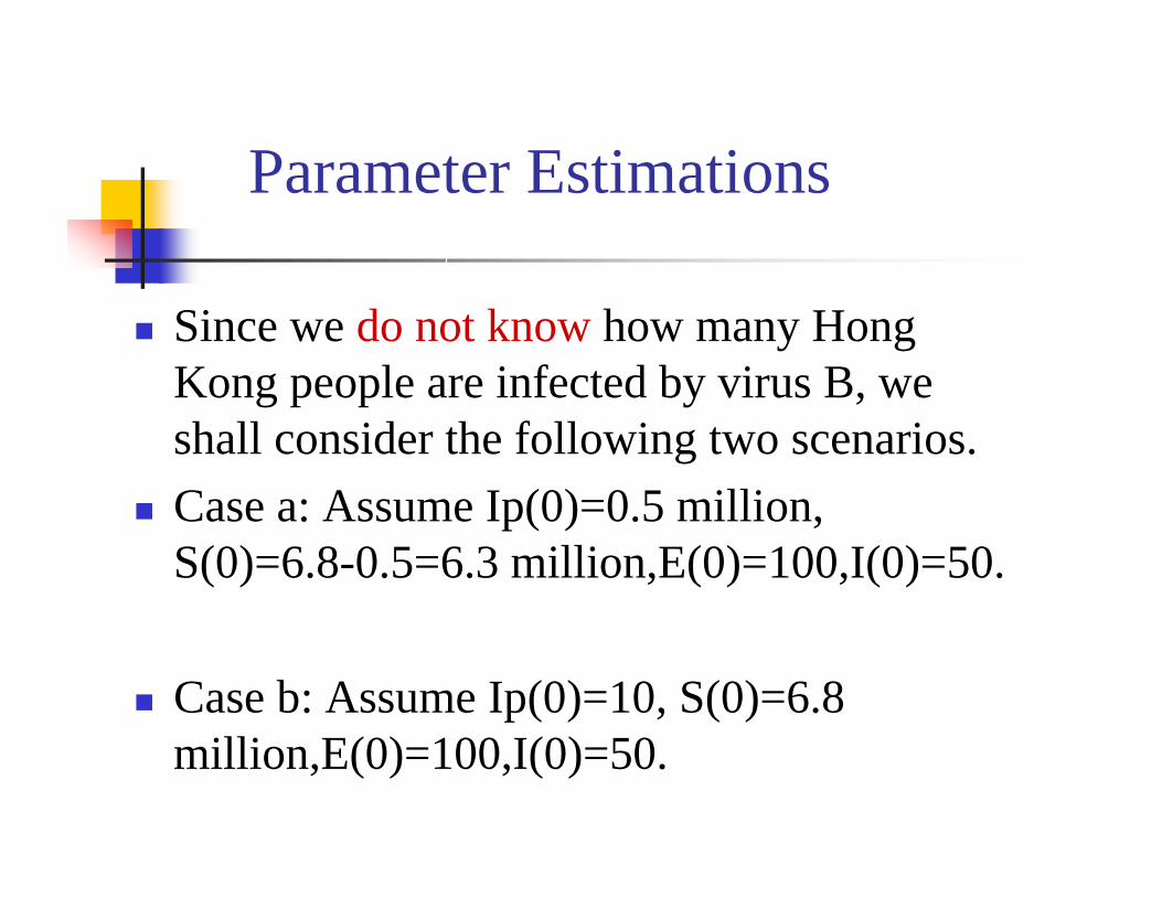
Parameter Estimations

Since we do not know how many Hong Kong people are infected by virus B, we shall consider the following two scenarios.Case a: Assume Ip(0)=0.5 million, S(0)=6.8-0.5=6.3 million,E(0)=100,I(0)=50.

Case b: Assume Ip(0)=10, S(0)=6.8 million,E(0)=100,I(0)=50.

We fit the model with the total number of confirmed cases from 17 March, 2003 to 10 May, 2003 (totally 55 days). The parameters are obtained by the gradient-based optimization algorithm.The resulting curve for R fits very well with

the observed total number of confirmed cases of SARS from the community.

Parameter Estimations

0

10

20

30

40

50

60

70

80

90

100

03/17

-03/19

03/23

-03/25

03/29

-03/31

04/04

-04/06

04/10

-04/12

04/16

-04/18

04/22

-04/24

04/28

-04/30

05/04

-05/06

05/10

-05/12

Num

ber o

f cas

es

ObservedExpected

Figure 3: Number of SARS cases in Hong-Kong community (and the simulated case “a”) per three days.

0

10

20

30

40

50

60

70

80

90

100

03/17

-03/19

03/23

-03/25

03/29

-03/31

04/04

-04/06

04/10

-04/12

04/16

-04/18

04/22

-04/24

04/28

-04/30

05/04

-05/06

05/10

-05/12

Num

ber o

f cas

esObservedExpected

Figure 4: Number of SARS cases in Hong-Kong community (and the simulated case “b”) per three days.

Parameter Estimations

Case a: Assume Ip(0)=0.5 million, S(0)=6.3 million,E(0)=100,I(0)=50.

r=10.19x10-8, r_p=7.079x10-8 .a=0.47,a_p=0.461,b=0.103.Estimated 1/a + 1/b = 11.83 (quite close to the observed 1/a+1/b= 10.12).

Parameter Estimations

Case b: Assume Ip(0)=10, S(0)=6.8 million,E(0)=100,I(0)=50.

r=10.08x10-8, r_p=7.94x10-8.a=0.52,a_p=0.12,b=0.105.Estimated 1/a + 1/b = 11.44 (quite close to the observed 1/a+1/b= 10.12).

Basic reproductive factor

R0 is the number of secondary infections produced by one primary infection in a whole susceptible population.Case a: R0=1.37.Case b: R0=1.32.

We define the basic reproductive factor R0as

R0=rS(0)/a.

ConclusionWe did not explore the intricacies of the mathematical solutions of this new epidemiological model, but, rather, tried to test with very crude hypotheses whether a new mode of transmission might account for surprising aspects of some epidemics.Unlike the SIR model, for the SEIRP model we cannot say that the epidemic is under control when the number of admission per day decreases. Indeed in the SEIRP models, it may happen that momentarily the number of people in the Infective class is low while the Exposed class is still high (they have not yet been infectious);

Thus the epidemic may seem stopped but will then be out of control again when in people in the Exposed class migrate to the Infected class and will start contaminating other people (especially if sanitary security policy has been relaxed). Thus an effective policy necessarily takes into account the time required for the Exposed (E) class to become infectious and will require zero new cases during all the period. The double epidemic can have a flat, extended peak and short tail compared to a single epidemic, and it may have more than one peak because of the latency so that claims of success may be premature.

This model assumes that a mild epidemic protects against SARS would predict that a vaccine is possible, and may soon be created.

It also suggests that there might exist a SARS precursor in a large reservoir, prompting for implementation of precautionary measures when the weather cools down.