WP/16/2015

NSE Working Paper 1

Mispricing in single stock futures:

Empirical examination of Indian markets

Shankar R.L. 2

Professor, Great Lakes Institute of Management, Chennai

Ganesh Sankar

Manager, Standard Chartered Scope International, Chennai

Kiran Kumar K

Associate Professor, Indian Institute of Management, Indore

June 2015

1The views expressed in the paper are those of the authors and do not necessarily reflect the opinion ofthe National Stock Exchange of India Ltd.

2Corresponding author. Email: shankar.rl@greatlakes.edu.in.

1

Mispricing in single stock futures:

Empirical examination of Indian markets

Abstract

We examine the dynamic relationship among liquidity, volatility and mispricing in sin-

gle stock futures. We use data from the National Stock Exchange of India, which is the

second largest global trading venue for such contracts. We compute mispricing bounds

using multi-regime models for over hundred stocks. The size of the mispricing window

- defined as the distance between these bounds - increases with decrease in liquidity.

Liquidity of the futures market has a larger impact on the size of the mispricing win-

dow compared to that of the spot market. After controlling for these liquidity effects,

the size of the mispricing window is found to increase with an increase in volatility.

This suggests that concerns related to margin calls and execution shortfalls dominate

the early exit options. Volatility has an asymmetrical effect on mispricing bounds.

We attribute this to short-sale constraints as they make early exit option less relevant

when the futures are underpriced.

Keywords: Mispricing in futures; liquidity; volatility; short sales; SETAR

JEL Classification: G13, G14, G15

2

1 Introduction

Classical no-arbitrage theories establish a linkage between the prices of a futures contract

and its underlying asset. Deviations from this relation, beyond a certain threshold, would

be eliminated by the actions of arbitrageurs. While these thresholds were traditionally

interpreted as a function of transaction costs, recent studies posit that these thresholds

could also be influenced by the strategic choices made by arbitrageurs (Liu and Longstaff,

2003; Kondor, 2009; Oehmke, 2009). However, very little is understood about how these

thresholds vary with market parameters. This paper examines how these thresholds are

affected by liquidity, volatility and short-sales constraints using data on single stock futures

from the National Stock Exchange (NSE) of India. Globally, NSE is ranked second in terms

of the number of trades in such contracts1.

To facilitate our empirical analysis, we posit that deviations in prices between a security

and its futures contract follow a multi-regime model. Specifically, mispricing is assumed to

fall under one of three regimes: (1) a regime mispricing is below a lower threshold; (2) a

regime where mispricing is above an upper threshold; or (3) an intermediate regime where

mispricing is between these bounds. We compute a model-free and a model-based estimate of

these thresholds. Estimating these bounds permits us to make several key inferences about

the drivers of path dependency in pricing errors.

Our central contributions are three-fold. First, we examine the impact of liquidity on mis-

pricing bounds. Oehmke (2009) postulates that liquidity is a key determinant of the speed

with which capital moves to arbitrage opportunities. He shows that for a given level of com-

petition, arbitrageurs would trade less aggressively when liquidity is low. Further, the level

1Source: 2010 World Federation of Exchanges Market Highlights

3

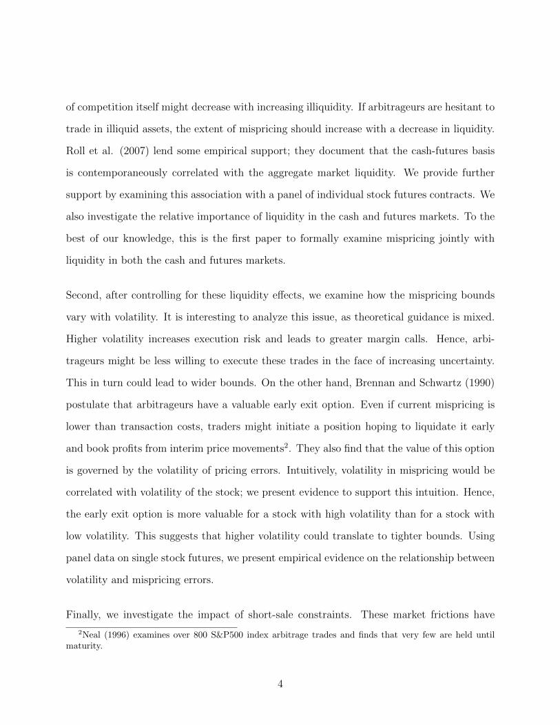
of competition itself might decrease with increasing illiquidity. If arbitrageurs are hesitant to

trade in illiquid assets, the extent of mispricing should increase with a decrease in liquidity.

Roll et al. (2007) lend some empirical support; they document that the cash-futures basis

is contemporaneously correlated with the aggregate market liquidity. We provide further

support by examining this association with a panel of individual stock futures contracts. We

also investigate the relative importance of liquidity in the cash and futures markets. To the

best of our knowledge, this is the first paper to formally examine mispricing jointly with

liquidity in both the cash and futures markets.

Second, after controlling for these liquidity effects, we examine how the mispricing bounds

vary with volatility. It is interesting to analyze this issue, as theoretical guidance is mixed.

Higher volatility increases execution risk and leads to greater margin calls. Hence, arbi-

trageurs might be less willing to execute these trades in the face of increasing uncertainty.

This in turn could lead to wider bounds. On the other hand, Brennan and Schwartz (1990)

postulate that arbitrageurs have a valuable early exit option. Even if current mispricing is

lower than transaction costs, traders might initiate a position hoping to liquidate it early

and book profits from interim price movements2. They also find that the value of this option

is governed by the volatility of pricing errors. Intuitively, volatility in mispricing would be

correlated with volatility of the stock; we present evidence to support this intuition. Hence,

the early exit option is more valuable for a stock with high volatility than for a stock with

low volatility. This suggests that higher volatility could translate to tighter bounds. Using

panel data on single stock futures, we present empirical evidence on the relationship between

volatility and mispricing errors.

Finally, we investigate the impact of short-sale constraints. These market frictions have

2Neal (1996) examines over 800 S&P500 index arbitrage trades and finds that very few are held untilmaturity.

4

a direct influence on our earlier predictions as the early exit option might be relevant only

when futures are overpriced. When they are underpriced, a trader might not be able to place

the initial trades - long futures, short stock - given the restrictions on short sales. Hence,

the effect of volatility on mispricing via the early exit option might be highly asymmetrical.

Further, short-sale constraints have impacts on mispricing that are more fundamental. For

instance, the lower bounds would be higher in magnitude compared to the upper bounds.

However, if a majority of arbitrage trades are executed by institutions that can sell stocks

from their existing holdings (as documented by Neal, 1996), these restrictions might not be a

major impediment. While extant studies examine the relations between variance, short-sale

constraints and pricing errors (Yadav and Pope, 1990, 1994; Fung and Draper, 1996), this

is the first study to provide direct evidence on how volatility and liquidity jointly vary with

the parameters that govern path dependency in mispricing.

In this study, we study mispricing in single stock futures using intra-day data from the

National Stock Exchange of India (NSE). Our findings can be briefly summarized as follows.

The size of the mispricing window increases with a decrease in liquidity. The liquidity of the

futures market has a larger impact on the size of the mispricing window compared to that of

the spot market. After controlling for liquidity effects, the size of the mispricing window is

found to increase with a increase in volatility. This suggests that concerns over margin calls

and execution shortfalls dominate the early exit options.

The examination of the impact on individual mispricing bounds offers greater insights.

Higher volatility is associated with the lower bound becoming more negative and the upper

bound becoming less positive. However, the former dominates the latter leading to a positive

association between volatility and the size of mispricing. These findings suggest that higher

volatility is associated with greater underpricing in futures contracts. We conjecture that

5

this result is driven by short-sale constraints. When futures are underpriced, an arbitrageur

would exploit the situation by going long futures and short stocks. If short selling is con-

strained, the trader might not be able to execute the trade. However, this does not mean

that the arbitrage opportunity would persist infinitely. If the extent of mispricing is very

high, traders might initiate a naked long futures position (Hull, 2014). In the face of high

volatility, such traders run a greater risk of margin call and might be reluctant to place such

bets. This leads to greater underpricing. Turning to the more fundamental effects of these

market frictions, the mean lower bound of mispricing is higher in magnitude than the mean

upper bound. This suggests that short-sale constraints also have an asymmetrical impact

on mispricing bounds .

The rest of this paper proceeds as follows. Section 2 provides an overview of Indian capital

markets and discusses our sample data. Section 3 elaborates on the empirical framework

adapted in the study and presents our main results. Section 4 concludes the paper.

2 Overview of Indian Markets and Data

Trading in the Indian derivatives markets is concentrated in one national exchange: the

National Stock Exchange (NSE) of India. It accounts for about 98% of the turnover in the

derivatives market3. The NSE commenced trading in equity derivatives in June 2000 with

the launch of index futures. Futures on individual stocks were introduced in November 2001.

As pointed by Vipul (2008), the market witnessed reasonable liquidity even during its initial

years. This could be partly attributed to the presence of an informal retail-driven forward

trading system that existed between 1972 and 2001 (Berkman and Eleswarapu, 1998). Stock

3Source: Website of Securities and Exchange Board of India (SEBI)

6

futures in India have recorded impressive growth since their inception; currently, the NSE is

ranked second in terms of the number of single stock futures contract traded, next only to

NYSE Liffe Europe.

In November 2001, the NSE introduced futures on 31 stocks. The NSE periodically adds

stocks to the derivatives segment based on their liquidity. The NSE computes the “quarter

sigma” order size for each stock; “quarter sigma” refers to the order size that is required to

cause a change in price equal to one-quarter of its standard deviation. Futures are introduced

on a stock if its quarter sigma is above a certain threshold. Our study begins from January

2007. As on this date, 170 stocks were traded in the futures segment. Of these, 30 stocks were

introduced during the last six weeks of 2006. We drop these newly introduced stocks from

our analysis to allow for a certain acclimatization phase. Further, we dropped an additional

set of 38 stocks that were either subsequently removed from the derivatives segment by the

NSE or merged in the underlying spot market. We are left with a sample of 102 stocks.

In selecting January 2007 as the start of our sample period, we have attempted to strike

a balance between the need to have a long sample period and the desire to have a wide

cross-section of stocks. We present the basic descriptive statistics for these stocks in Table

1. As is evident, the futures market witnessed higher turnover than the underlying cash

market.

The Securities and Exchange Board of India (SEBI) banned short selling in Indian bourses

in March 2001. This ban was not applicable to retail investors. In December 2007, the

SEBI allowed institutional investors to short sell stocks. However, naked short-selling was

strictly prohibited for all market participants. Investors were required to honour their de-

livery commitments mandatorily. To create a vibrant lending market, the SEBI instituted

a Securities Lending and Borrowing (SLB) scheme. Traders had to borrow the shares they

7

were short-selling from SLB. The SLB market was introduced by the National Securities

Clearing Corporation Limited in April 2008. The tenure of SLB contracts was initially lim-

ited to a week. While there were a few trades in the SLB market during the first two weeks,

there were practically no trades subsequently4. A popular Indian daily the slammed SLB,

calling it “dysfunctional [with] an average lending quantity of zero”.5

To enhance participation, the tenor of SLB contracts was extended to a month. However,

this move also failed to excite the market participants. During the calendar year 2009,

less than 0.5 million shares were lent or borrowed in the SLB market through a total of

80 transactions.6 In January 2010, the tenor of SLB contracts was extended to a year.

Subsequently, interest among market participants picked up in the second half of 2010. Over

the subsequent years, multiple regulatory reforms were introduced, which included allowing

insurance firms to participate in this market. Courtesy these reforms, the liquidity in these

markets has increased substantially. Our study spans the calendar years 2007-2009. During

this period, either short-selling was banned (January 2007 - April 2008) or the extent of

short-sales was truly negligible (April 2008 - December 2009).

Data source: Our data source is the high frequency database obtained from the NSE.

This database contains time-stamped intraday prices of all the transactions in the spot and

derivatives segment. Since intraday prices are prone to data errors, we follow Zhou (1996)

and remove spurious observations from our raw datasets. We compare each transaction

price with the median of three prices before and after the transaction. The observed price is

removed if it falls outside a threshold distance from the median by 5%. For the first and the

last observations, we take the median of three succeeding and three preceding transaction

prices respectively.

4SEBI to extend securities lending tenor, LiveMint, 04 August 2008)5Why ban short selling? Financial Express, 26 October 20086After 2 years, stock lending booms on reverse arbitrage, DNA India, 13 September 2010

8

We sample prices every five minutes. While a higher frequency would introduce greater

microstructural noise, a lower frequency might not permit us to efficiently capture the path

dependencies in mispricing. For both the futures and the spot market, we take the last price

observed in each five minute window. The time-stamped five minute samples prices from

both these markets are merged to form a matched time series. This time series is in turn

used to construct our mispricing series. The theoretical futures price (Ft) is computed using

the classical cost of carry relationship (Cornell and French, 1983):

Ft = (St − PV (D))er(T−t) (1)

where St is the spot price, PV (D) is the present value of the dividend discounted from the

ex-dividend date; r is the 14-day Mumbai Interbank Offer Rate (MIBOR); and (T − t) is the

time till maturity of the contract. Spot price is adjusted for dividends when the ex-dividend

date falls during the tenure of the contract. We use the dividend data provided by the NSE

which contains both the announcement and ex-dividend dates. MIBOR is a polled rate that

reflects the cost for unsecured borrowing and lending in the interbank market (also known

as the call market). MIBOR for various tenures is published daily by the NSE; we use the

14-day tenure since the average maturity of the contracts used for the analysis is around two

weeks.

On any given day, contracts with three different maturities are available for trading - one that

expires in the same month, one that expires the next month and one that expires the month

after. Trading in futures at the NSE tends to be concentrated in same-month contracts

(Vipul, 2009). Hence, we consider only these contracts in constructing the mispricing series.

However, to control for the well-documented expiration week effects, during the expiry week,

we consider contracts that mature in the subsequent month.

9

We then compute relative mispricing following Yadav and Pope(1994):

πt =FMt −Ft

St(2)

where FMt is the market price of the futures contract. To make cross-sectional inferences

meaningful, we normalize the mispricing with the prevailing spot price. The basic descriptive

statistics of this mispricing series are provided in Table 1. We find that the relative mispricing

varied between a fairly wide range of −273 basis points to +16 basis points. The median

mispricing is −12 basis points. Based on unreported tests, we reject the hypothesis that the

median is zero.

3 Research design and results

Our empirical analysis proceeds as follows. First, we discuss the core econometric framework

used in this study, i.e., multi-regime models. Second, we examine how short-sale constraints

affect the path dependency of pricing errors. Third, we present the results for our liquidity-

sorted portfolios. Fourth, we elaborate on our volatility measure and discuss its impact on

futures mispricing. Fifth, we examine the joint effect of liquidity and volatility by including

liquidity as an explanatory variable in our panel models. Finally, we present tests that

examine the robustness of our central findings.

3.1 Multi-regime models:

In an efficient market with no frictions, the prices of futures and the underlying asset are

linked through a no-arbitrage relation. However, arbitrageurs might find it economically

10

attractive to initiate trading positions only if the deviation from this relation exceeds a

certain threshold. These thresholds could be determined by transaction costs (Modest and

Sundaresan, 1983) and early liquidation value (Brennan and Schwartz, 1990), among other

factors. Recent studies postulate that this interval could also be endogenously influenced by

the strategic choices made by arbitrageurs (Liu and Longstaff, 2003; Kondor, 2009; Oehmke,

2009). It is then fairly intuitive to model mispricing in these contracts using a multiple-

regime model such as the Self-Exciting Threshold Auto-Regression (SETAR) model. Yadav

et al.(1994) provide an excellent overview of this class of models and their applicability to

modeling the price difference of equivalent assets such as stocks and their futures. Here, we

briefly review this approach. Mispricing (as defined in equation (2) is assumed to follow a

multi-regime process:

πt = αL +∑6

i=1 φiLπt−1 + εt, πt−1 < κL

= αM +∑6

i=1 φiMπt−1 + εt, κL < πt−1 < κM

= αH +∑6

i=1 φiHπt−1 + εt, πt−1 > κH

(3)

We first define two mispricing bounds: a lower mispricing bound (denoted by LMB or κL)

and an upper mispricing bound (denoted by UMB or κH). If the mispricing during the

last period, πt−1, is between κL and κH , the current mispricing πt is assumed to follow a

AR(6) process with persistence of φi=1...6M . However, if the past mispricing is lesser than κL

or greater than κH , πt follows a AR(6) process with the persistence co-efficients being φi=1...6L

and φi=1...6H respectively.

While it is possible to specify threshold values exogenously (say as a function of transaction

costs), it might be more appropriate to estimate them simultaneously for multiple reasons.

First, the option to liquidate early is valuable to traders. Hence, even if the current level of

mispricing is below the transaction costs, arbitrageurs would initiate trades if they believe

11

that the mispricing would reverse prior to maturity. Hence, it might be inappropriate to

constrain these thresholds to transaction costs. Second, regulatory constraints such as short-

sale constraints could have an asymmetrical impact on thresholds. For instance, we expect

κL to be higher in magnitude than κH . This is because when futures are overpriced, it is

easier to set up the arbitrage trades; on the other hand, when they are underpriced, arbitrage

could be difficult as shorting stocks is not permitted. However, it is not feasible to a priori

quantify the degree of asymmetry. Therefore, we determine the thresholds simultaneously.

It is worth clarifying three estimation issues that arise in estimating the model specified

in Equation 3. First, since the thresholds are not specified a priori, we use a grid search

procedure over a range of threshold values to obtain an estimate that minimizes the residual

sum of squares . Second, we have assumed that the variable that determines the current

regime is the one-period lagged value of mispricing. In assuming this and not simultaneously

estimating the optimal lag length, we follow Yadav et al. (1994). Working with data sampled

at 15-minute intervals, they state that one lag is sufficient to capture any likely delay in

arbitrage activity. While we work with a finer frequency (5-minute intervals), we believe

that the underlying rationale still holds. Third, mispricing in each regime is assumed to

follow a AR (6) process. While the appropriate specification could be different for each firm,

we find that a AR(6) specification is suitable for most cases. Further, this consistency greatly

enhances the presentation and interpretation of our final results. However, the assumption of

six lags prevents us from making inferences about the persistence of mispricing; it is difficult

to single out the individual effect of any one lag. Additionally, we check the robustness of

our results to this specification by estimating the model with lower AR lags.

We choose the estimation window for the SETAR model to be a week, with the week running

from Monday to Friday. For each firm, we estimate the model every week using mispricing

12

computed at five minute intervals. This yields the estimates of various parameters for each

firm-week combination. For each parameter, we then compute a firm-specific mean by aver-

aging its weekly estimates. Next, we estimate a cross-sectional mean across all firm-specific

means of this parameter. We report this mean along with the t-statistic against the two-sided

hypothesis that the mean is zero. These results are presented in Table 2.

The mean of κL and κH for the stocks in our sample is −39 and −10 basis points respectively;

both these estimates are significant at conventional levels of significance. The negative sign

on the upper bound might be surprising. If one were to assume that these bounds reflect

transaction costs, this should be a positive number. To ensure that this result is not driven by

issues with the model specification in (3), we compute model-free estimates of these bounds

in subsequent sections, and we find that the result holds.

Table 3 presents the results for two sub-sample periods. “Pre-SLB” refers to the period

prior to the introduction of the SLB contracts (January 2007 - April 2008), and “Post-SLB”

refers to the subsequent period (May 2008 - December 2009). The width of the mispricing

interval remains the same for both the sub-periods. κL and κH are statistically significant

and negative across both periods. While both κL and κH are less negative in the latter period,

the width of the mispricing band is similar across both the periods. This suggests that the

early version of SLB was not effective; this was perhaps due to the lack of participation in

these markets.

3.2 Liquidity and mispricing:

To assess the impact of liquidity on futures mispricing, we sort the stocks by their liquidity.

Specifically, we use a measure of the impact cost provided by the NSE for the underlying

13

market. Impact cost refers to the percentage price movement caused by a specific order size

(currently INR 100,000). 7 We select a pre-sample period spanning twelve months between

January 2006 and December 2006 and compute the average impact cost over this period.

Stocks are then sorted based on their impact cost; IC1 refers to the stocks with the lowest

impact cost (i.e., the most liquid stocks). In Table 4, we report the cross-sectional average

of the firm-specific means for the firms in each sub-sample. The average impact cost for

the firms in the most liquid category is 8.3 basis points; this is about half that for the least

liquid stocks in our sample. Mean mispricing for all the groups is negative; it is highest in

magnitude for the most liquid stocks.

Table 4 presents the results of SETAR estimates for the various sub-samples. Oehmke (2009)

postulates that arbitrageurs would be hesitant to trade in illiquid assets. Hence, we should

expect the width of the mispricing intervals to be higher for these stocks. Our findings

provide weak evidence for this hypothesis: the most liquid stocks have a window of 27 basis

points, compared to 29 basis points for the least liquid stocks in our sample. While the

difference is statistically significant at 99% significance level (based on unreported tests),

its economic significance is not immediately apparent. In subsequent sections, we provide

further insights by including contemporaneous liquidity as an explanatory variable in our

regression framework.

Examining the individual thresholds offers more interesting insights. The lower threshold

(κL) for the most liquid stocks is −52 basis points; in comparison, κL for the least liquid

stocks is −20 basis points. The difference is both statistically and economically significant.

We can only speculate about the reason for this difference. This is perhaps driven by short-

7To compute impact cost, NSE chooses four fixed ten-minute windows spread across the trading day.From each of these intervals, it randomly chooses an order book snapshot. This snapshot is then used asinput for calculating he impact cost. This information is published at the end of each calendar month. Thisinformation is published at the end of every calendar month.

14

sale constraints: the risk of initiating a long futures position without an offsetting short

position in the cash market is higher for liquid stocks, particularly if the underpricing in

futures is driven by differential rates of information diffusion. This possibility presents an

interesting line of research, which we leave to future work. For portfolios sorted on liquidity,

we also undertake year-wise analysis of SETAR the estimates; the results are qualitatively

similar to those of full sample and are, hence, not reported.

A potential concern with our analysis is that our inferences are based on estimates of the SE-

TAR model. To alleviate this concern, we additionally compute simple model-free estimates

of LMB and UMB. We compute mispricing from data sampled at five-minute intervals and

define the model-free upper mispricing bound (MFUMB) as the kth percentile observation

and the model-free lower mispricing bound (MFLMB) as the 100−kth percentile. We permit

k to take multiple values such as 10, 20 or 25. Table 6 presents these estimates for both

the full sample as well as the liquidity-sorted sub-samples. As would be anticipated, none of

these MF bounds perfectly match the SETAR estimates. Of greater interest to us are the

relative values across the sub-samples, the results remain qualitatively similar: liquid assets

have narrower bands of mispricing and lower MFLMB. Hence, our central results are robust

to measurement of mispricing bounds.

3.3 Volatility and mispricing:

Volatility could impact the size of the mispricing window through two channels. First, higher

volatility could increase the risk of margin calls and execution shortfalls. Traders might then

wait for the window to widen before initiating their arbitrage trades. This might lead to

wider mispricing bands. On the contrary, higher volatility could increase the value of the

early exit option. Even if current mispricing is lower than transaction costs, traders might

15

initiate a position hoping to liquidate it early and book profits from interim price movements.

Brennan and Schwartz (1990) postulate that the value of this early exit option is governed by

the volatility of pricing errors. We hypothesize that the volatility in mispricing is positively

correlated with the volatility of the stock. Under this assumption, higher volatility could

lead to tighter mispricing bands. Given these divergent views, it is interesting to examine

the impact of volatility.

We first test our hypothesis that the volatility of stock is positively correlated with that

of mispricing in futures contract. To be specific, for each stock, we compute the realized

volatility over the entire sample period. Realized volatility is measured as the square-root of

realized variance, which is defined below in (5). We also compute the volatility in mispricing

sampled at five minute intervals. For each stock, we then compute the correlation between

these two measures. We present the histogram of these correlations in Figure 1. All the

correlation measures are positive; the minimum is 0.22 and the maximum is 0.72 (based on

untabulated results). The mean and the median of this series are 0.50 and 0.51 respectively.

We conclude that these series are positively correlated. Hence, higher volatility of stocks

could potentially lead to greater value of early exit options.

Next, we next examine the association between volatility and the mispricing thresholds using

panel regression techniques. The estimate of the mispricing bounds is used as the depen-

dent variable, and the contemporaneous weekly realized variance is the primary explanatory

variable. The full specification is presented in Equation 4:

yi,t = α + βRVi,t + γyi,t−1 + θWTMt + δDSLB + εi,t (4)

where yi,t refers to the mispricing threshold estimated for firm i for week t obtained using

the SETAR models; RVi,t refers to the realized variance for firm i for week t, and yi,t−1

16

refers to the lagged estimate of the dependent variable. We use contemporaneous volatility

in this estimation, as we are interested in examining the association between volatility and

mispricing bounds. Fung and Draper (1996) and Chen et al. (1995) use a similar time-series

specification that employs a contemporaneous volatility estimate to analyze the impact of

volatility on pricing errors in index futures.

The model in Equation 4 is estimated separately for the two bounds: κL, κH and for the

mispricing band: κH − κL. As the futures approach maturity, the futures prices converge to

the stock price; hence, the arbitrage bounds tend to decline (MacKinlay and Ramaswamy,

1988). To capture this, we include week to maturity (WTM) as an independent variable.

Further, we add a dummy for SLB introduction: DSLB takes a value of 0 for the period prior

to the introduction of SLB and 1 for the period after. We use the panel data technique with

firm fixed effects; all standard errors are corrected as in Petersen (2009).

It is now well documented that the realized variance measures computed using intraday data

yield a superior estimate of the actual return variance as compared to those computed using

daily returns (Andersen and Bollerslev, 1998; Andersen et.al., 2001; Barndoff-Nielsen and

Shephard, 2002). If we denote the intra-day log return over an interval i as ri and assume

that there are N such equally spaced intervals in a given period [t, T ], then the realized

variance (RVt,T ) for this period is computed as

RVi,t =∑N

i=1 r2i

(5)

Realized variance defined as in Equation 5 is a consistent estimator of quadratic variation in

the asymptotic limit. In reality, it is neither possible nor desirable to sample continuously;

it is not desirable to do so because of the noise that arises from microstructural effects such

as bid-ask bounce. The optimal interval for sampling intraday returns has attracted much

17

attention; Jian and Tiang (2005) provide a good summary of this literature. We adapt

their recommendation and sample returns at five-minute intervals and correct for first order

autocorrelation in returns.

Table 7 presents the results of the panel regression for the estimates of the mispricing bband,

κH − κL. An increase in the weekly variance of stock returns is associated with an increase

in the mispricing interval for the entire sample. The lagged value of the mispricing band is

significant; evidently, mispricing bands are persistent. Week-to-maturity (WTM) is signif-

icant and is estimated with the correct sign. As we approach the maturity of the contract

(i.e., as WTM decreases), the mispricing band decreases. We also estimate the full model

specified in equation 4 for the liquidity-sorted subsamples. The results are qualitatively sim-

ilar: the mispricing band increases with an increase in volatility. Our findings suggest that

the risk of margin calls and execution shortfalls dominate the value of the early exit option

in determining the sensitivity of mispricing band to volatility.

Short-sale constraints could cause volatility to have an asymmetrical impact on the lower

and upper bounds. To investigate this effect, we estimate the model in equation 4 with the

estimates of the mispricing bounds as the dependent variable. These results are tabulated

in Table 8. For the sake of brevity, we report only the estimates for β, the co-efficient on

realized variance. The lower bound, κL, decreases with an increase in volatility; i.e., higher

volatility is associated with κL becoming more negative. The impact of the variance on

the upper bound, κH , is equally interesting: the upper bound also decreases with volatility;

however, the decrease in κH is lesser than that in κL. This leads to an effective widening of

the mispricing window. The explanatory power of these regressions is more than 50%.

Table 8 also presents the results for the various liquidity-sorted subsamples. The results

remain qualitatively similar across these groups, suggesting that our earlier results are robust

18

to variations in the liquidity of the underlying stocks. While comparing the impact of

volatility across these groups, we do not find any discernible trend across the liquidity groups.

To gauge the sensitivity of our results to the definition of mispricing bounds, we re-estimate

the model with our model-free estimate of LMB and UMB. For the sake of brevity, we

report the results for bounds corresponding to the 75th percentile and the 25th percentile

respectively. These results are presented in Table 9. A 1% increase in weekly variance

leads to a 9.6 basis points (bp) increase in the mispricing interval, 12.1 bp decrease in LMB

and 3.34 bp decrease in UMB. These results are mostly consistent with our earlier findings.

Hence, we conclude that our results are robust to measurement of mispricing bounds.

3.4 Joint specification of liquidity and volatility

In the earlier section, we used liquidity measured at the beginning of our sample period to

sort the samples. To better capture the joint dynamics of liquidity and volatility, we extend

our panel regressions to include a measure of contemporaneous liquidity as an explanatory

variable. To be specific, we include the impact costs for both the cash and the futures

markets. This also permits us to examine whether one has a more dominant association

with mispricing compared to the other.

To construct the time-series of the liquidity measures, we use order book data provided by

the NSE. The NSE provides snapshots of the order book at five different times during the

day. This contains all the relevant information about the sitting limit orders such as limit

price and quantity. We use the snapshot provided at 14:00 hours for our analysis. We first

define the benchmark price as the average of the best bid and the best ask prices. We then

define the execution price of an order as the weighted average price at which the order is

19

executed. Impact cost is measured as the difference between the execution price and the

benchmark price; relative impact cost (RIC) is the impact cost divided by the benchmark

price. We compute RIC for a buy order and a sell order, each of value INR 500,000. The

RIC for a stock for a day is defined as the average RIC of the buy and the sell order. The

RIC for a week is computed as the weekly average of the daily RICs.

To study the joint dynamics of volatility, liquidity and the mispricing window, we extend

our panel regression framework in equation 4 by including contemporaneous liquidity as an

additional explanatory variable. The full specification is presented in equation 6:

yi,t = α + βRVi,t + ωCRICCi,t + ωFRIC

Fi,t + γyi,t−1 + θWTMt + δDSLB + εi,t (6)

where RICCi,t and RICF

i,t denote the relative impact cost in the cash and the futures market

respectively. While we estimate the model in equation 6 for all the parameters, for the sake

of brevity we present only the results for the mispricing interval: κH − κL in Table 10.

We make several interesting inferences. First, the relative impact costs in the cash and the

futures markets are significant; they also have the correct sign. An increase in impact costs

leads to a wider mispricing window. Second, the RIC in the futures market has a larger

impact compared to that in the cash market. This suggests that arbitrageurs are more

concerned about the lack of liquidity in the futures market. Third, even after controlling

for liquidity in the cash and futures market, we find volatility to be positive and significant.

Hence, our earlier results regarding the association between volatility and mispricing survive

the inclusion of contemporaneous liquidity measures.

20

3.5 Robustness tests

In this section, we discuss three additional robustness tests that we conducted. For reasons

of brevity, we do not tabulate these results in this paper. First, we examine the robustness of

our results to the cost of carry model and the interest rates used therein. We use basis as our

dependent variable; basis is defined as the difference between the market prices of a futures

contract and its underlying, normalized by the price of the underlying. Since basis does not

take holding costs into account, a priori we expect both the bounds - LMB and UMB - to be

higher. However, the mispricing band (UMB - LMB) should remain largely unaltered. Based

on untabulated results, we find that individual bounds are indeed higher. The estimated

bands for basis and mispricing are almost equal. Further, we find that volatility has similar

impact on the parameters that govern path dependency in basis. Hence, our earlier inferences

are not influenced by interest rates or more generally the cost of carry model.

Second, we examine whether our results are sensitive to the assumption that mispricing

follows a AR(6) process in various regimes. Instead, we assume that mispricing follows a

AR(1) process. We find that the actual specification of the mispricing process in each regime

does not materially influence our results. Third, in our joint analysis of liquidity, volatility

and mispricing, we used Relative Impact Cost (RIC) as a proxy for liquidity. To verify

whether our results are sensitive to this proxy, we use an alternate measure of liquidity,

namely Relative Quoted Spread (RQS). Quoted spread is defined as the difference between

the best bid and the best ask price; RQS is quoted spread scaled by the average of the best

bid and the best ask prices. We find that our key inferences remain unaffected by the choice

of liquidity proxy.

21

4 Conclusions

In this article, we undertake a comprehensive investigation of the relationship between liq-

uidity, volatility and path dependency of mispricing in single stock futures. We use data from

the National Stock Exchange (NSE) of India, which is globally ranked second in terms of

trades in stock futures. The high liquidity in these markets permits us to examine a number

of interesting hypotheses. First, the size of the mispricing window increases with a decrease

in liquidity. Second, the liquidity of the futures market has a larger impact compared to

that of the spot market. Third, even after controlling for these liquidity effects, the size of

the mispricing window increases with an increase in volatility. These findings suggest that

concerns over margin calls and execution shortfalls dominate the early exit options.

Examining the mispricing bounds individually offers further insights. Higher volatility is

associated with the lower bound becoming more negative and the upper bound becoming

less positive. However, the former dominates the latter leading to our earlier finding that

an increase in volatility is associated with an increase in mispricing bands. We conjecture

that this result is driven by short-sale constraints. When the futures are underpriced, an

arbitrageur would respond by initiating a long position in the futures contract and a short

position in the cash market. However, if short selling is constrained, the trader might not be

able to simultaneously execute these trades. While he could initiate a naked long position,

the concerns about margin calls would be high. Hence, higher volatility pushes the lower

bound even further down.

22

References

[1] Andersen, T.G., and T. Bollerslev (1998), Answering the Skeptics: Yes, Standard

Volatility Models Do Provide Accurate Forecasts, International Economic Review, 39,

885-905.

[2] Andersen, T.G., T. Bollerslev, F. X. Diebold, and H. Ebens (2001), The Distribution

of Realized Stock Return Volatility, Journal of Financial Economics, 61, 43-76.

[3] Barndorff-Nielsen, O., and N. Shephard (2002), Econometric Analysis of Realised

Volatility and Its Use in Estimating Stochastic Volatility Models, Journal of Royal

Statistical Society, 64(B), 253-80.

[4] Berkman,H., and V.R. Eleswarapu (1998), Short-term traders and liquidity: a test using

Bombay stock exchange data, Journal of Financial Economics, 47, 339-355.

[5] Brennan, M., and E. Schwartz (1990), Arbitrage in stock index futures , Journal of

Business, 63(1), S7-S31.

[6] Chen, N., C.J.Cuny, and R.A. Haugen (1995), Stock volatility and the levels of the basis

and open interest in futures contracts, Journal of Finance, 50(1), 281-300.

[7] Cornell, B., and K.R. French (1983), The pricing of stock index futures, Journal of

Futures Market, 3, 1-14.

[8] Fung, J. K. W., and P. Draper (1999), Mispricing of index futures contracts and short

sales constraints, Journal of Futures Market, 19, 695-715.

[9] Hull, J.C. (2014), Options, futures and other derivatives, Prentice Hall, USA.

23

[10] Jiang, G. J., and Y. S. Tian (2005), The Model-Free Implied Volatility and Its Infor-

mation Content, Review of Financial Studies, 18(4), 1305-42.

[11] Kondor, P. (2009), Risk in Dynamic Arbitrage: The Price Effects of Convergence Trad-

ing, The Journal of Finance , 18(4), 64, 631-655 .

[12] Liu, J., and F.A. Longstaff (2004), Losing money on arbitrage: Optimal dynamic port-

folio choice in markets with arbitrage opportunities, Review of Financial Studies, 17(3),

611-41.

[13] MacKinlay, A.C., and K. Ramaswamy (1988), Index-futures arbitrage and the behavior

of stock index futures prices, Review of Financial Studies, 1, 137-158.

[14] Modest, D.M., and M. Sundaresan (1983), The relationship between spot and futures

prices in stock index futures markets: Some preliminary evidence, Journal of Futures

Market, 3, 15-41.

[15] Neal, R. (1996), Direct Tests of Index Arbitrage Models, The Journal of Financial and

Quantitative Analysis, 31, 541-562.

[16] Oehmke, M. (2009), Gradual Arbitrage, Working paper, Columbia University.

[17] Roll, R., E.Schwartz, and A.Subrahmanyam (2009),Liquidity and the Law of One Price:

The Case of the Futures-Cash Basis, The Journal of Finance , 62(5), 2201-34

[18] Vipul (2008), Cross-Market Efficiency in the Indian Derivatives Market: A Test of Put

Call Parity, Journal of Futures Markets, 28(9), 889-910.

[19] Vipul (2009), Box-Spread Arbitrage Efficiency of Nifty Index Options: The Indian

24

Evidence, Journal of Futures Markets, 29(6), 544-62.

[20] Yadav, P. K., and P. F. Pope (1990), Stock index futures arbitrage: International

evidence. Journal of Futures Market, 10, 573-603.

[21] Yadav, P. K., and P. F. Pope (1994), The Impact of Short Sales Constraints on Stock

Index futures Prices Evidence From FT-SE 100 Futures, The Journal of Derivatives,

1(4), 15-26.

[22] Yadav, P.K., P.F.Pope, and K.Paudyal (1994), Threshold autoregressive modeling in

finance: The price difference of equivalent assets, Mathematical Finance, 4, 205-21.

[23] Zhou, B. (1996), High-frequency data and volatility in foreign-exchange rates. Journal

of Business & Economic Statistics, 14(1), 45-52.

25

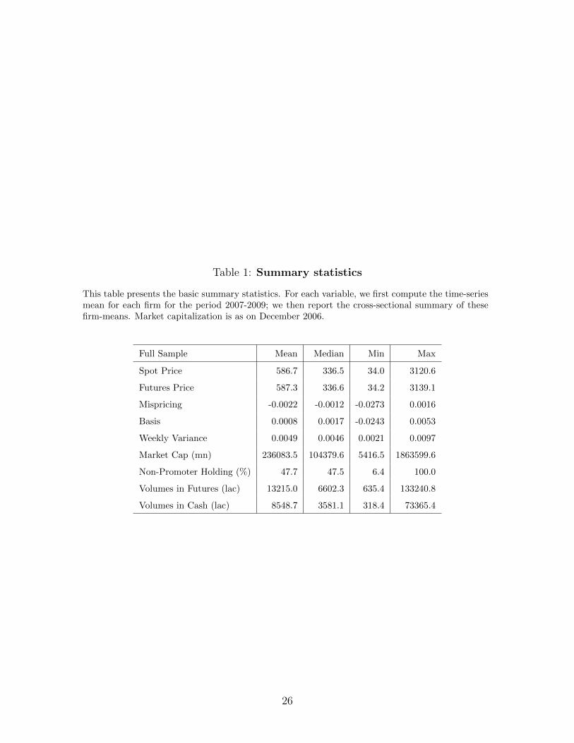
Table 1: Summary statistics

This table presents the basic summary statistics. For each variable, we first compute the time-seriesmean for each firm for the period 2007-2009; we then report the cross-sectional summary of thesefirm-means. Market capitalization is as on December 2006.

Full Sample Mean Median Min Max

Spot Price 586.7 336.5 34.0 3120.6

Futures Price 587.3 336.6 34.2 3139.1

Mispricing -0.0022 -0.0012 -0.0273 0.0016

Basis 0.0008 0.0017 -0.0243 0.0053

Weekly Variance 0.0049 0.0046 0.0021 0.0097

Market Cap (mn) 236083.5 104379.6 5416.5 1863599.6

Non-Promoter Holding (%) 47.7 47.5 6.4 100.0

Volumes in Futures (lac) 13215.0 6602.3 635.4 133240.8

Volumes in Cash (lac) 8548.7 3581.1 318.4 73365.4

26

Table 2: SETAR estimates

This table reports the estimates of the mispricing bounds and persistence parameters obtained fromthe SETAR model in equation 2. The table also reports the mean of the mispricing band (measuredas κH - κL). t-statistics are presented in parentheses.

Parameter Estimate t-stat

κL -0.0039 -57.04

κH -0.0010 -17.99

κH - κL 0.0028 127.79

φ1L 0.3399 175.21

φ2L 0.0871 34.66

φ3L 0.0922 58.32

φ4L 0.0526 32.64

φ5L 0.0502 29.21

φ6L 0.027 18.29

φ1M 0.3279 145.67

φ2M 0.089 5.07

φ3M 0.107 58.87

φ4M 0.0717 40.02

φ5M 0.0589 33.40

φ6M 0.045 25.57

φ1H 0.3197 58.55

φ2H 0.0578 20.06

φ3H 0.1005 26.20

φ4H 0.076 4.78

φ5H 0.0676 7.15

φ6H 0.0367 24.12

27

Table 3: SETAR estimates: Subsample analysis

This table reports the estimates of the mispricing bounds obtained from the SETAR model inequation 2 for two periods in our sample: Pre-SLB and Post-SLB. t-statistics are presented inparentheses.

Pre- SLB Estimate t-stat

κL -0.0053 -8.28

κH -0.0021 -3.84

κH − κL 0.0030 12.29

Post- SLB Estimate t-stat

κL -0.0039 -56.74

κH -0.0010 -17.83

κH − κL 0.0028 127.32

28

Table 4: Summary statistics for liquidity-sorted sub-samples

This table presents the basic summary statistics for the stocks that are sorted based on their liquidity,measured here using impact cost. IC1 refers to the stocks with the lowest impact cost, i.e., the mostliquid stocks in our sample. For each variable, we first compute the time-series mean for each firm forthe period 2007-2009; we then report the cross-sectional summary of these firm-means for differentliquidity groups. Market capitalization is as on December 2006.

IC1 IC2 IC3

Spot Price 907.1 399.3 453.6

Futures Price 907.5 399.6 455.0

Mispricing -0.0036 -0.0027 -0.0003

Basis -0.0004 0.0003 0.0026

Weekly Variance 0.0039 0.0047 0.0058

Impact Cost 0.0832 0.1299 0.1917

Market Cap (mn INR) 504932.1 153307.3 50011.2

Volumes in Futures (mn) 2667.8 780.3 516.5

Volumes in Cash (mn) 1706.8 513.2 344.7

29

Table 5: SETAR estimates for liquidity-sorted sub-samples

This table reports the estimates of the mispricing bounds and persistence parameters obtained fromthe SETAR model in (2) for the different liquidity-based sub-samples. IC1 refers to the stocks withthe lowest impact cost, i.e., the most liquid stocks in our sample. This table also reports the mean ofthe mispricing band (measured as κH - κL) and the difference between the persistence of mispricingin the upper and lower regimes. We also report the values for each year in our sample. t-statisticsare presented in parentheses.

κL κH κH − κL

IC1 -0.0052 -0.0025 0.0027

(-44.77) (-25.45) (76.35)

IC2 -0.0043 -0.0014 0.0029

(-32.41) (-12.78) (72.85)

IC3 -0.0020 0.0009 0.0029

(-21.48) (13.10) (72.69)

30

Table 6: Model-free estimate of mispricing bounds

This table reports the mispricing at various percentiles for the full sample and for different liquidity-sorted sub samples. IC1 refers to the stocks with the least impact cost, i.e., the most liquid stocks inour sample. This table also shows how the mispricing band, defined with respect to three differentpercentile levels, varies across the liquidity-based sub-samples. For each group, we report the cross-sectional average of the mispricing bounds and bands.

Full IC1 IC2 IC3

10% -0.0062 -0.0072 -0.0066 -0.0047

20% -0.0047 -0.0060 -0.0052 -0.0030

25% -0.0042 -0.0055 -0.0046 -0.0024

75% -0.0001 -0.0017 -0.0005 0.0019

80% 0.0003 -0.0013 -0.0001 0.0024

90% 0.0015 -0.0003 0.0011 0.0037

Mispricing band

90-10% 0.0077 0.0069 0.0077 0.0084

80-20% 0.0051 0.0047 0.0051 0.0054

75-25% 0.0040 0.0037 0.0041 0.0043

31

Table 7: Impact of variance on mispricing band

This table reports how the mispricing band is affected by weekly variance after controlling forits lagged value, week to maturity (WTM) and SLB dummies (refer equation 4). We report theestimates obtained using panel regression techniques along with the t-statistics (in parentheses). Wereport the value for the full sample and for different liquidity-sorted sub samples. IC1 refers to thestocks with the least impact cost (i.e, the most liquid stocks in our sample).

Weekly Variance Lag WTM DSLB Intercept R-Sq

Full Sample 0.1006 0.1932 0.0001 -0.0003 0.0017 0.198

(10.19) (12.35) (7.69) (-6.22) (24.16)

IC1 0.0850 0.2186 0.0002 -0.0002 0.0014 0.1474

(6.00) (7.94) (7.42) (-3.24) (11.60)

IC2 0.1054 0.1845 0.0001 -0.0006 0.0019 0.2397

(6.07) (7.20) (3.83) (-7.66) (16.65)

IC3 0.1042 0.1760 0.0001 0 0.0017 0.2036

(7.03) (6.75) (2.23) (0.63) (14.02)

32

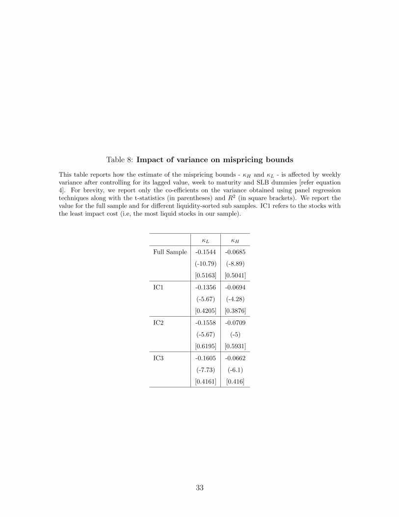
Table 8: Impact of variance on mispricing bounds

This table reports how the estimate of the mispricing bounds - κH and κL - is affected by weeklyvariance after controlling for its lagged value, week to maturity and SLB dummies [refer equation4]. For brevity, we report only the co-efficients on the variance obtained using panel regressiontechniques along with the t-statistics (in parentheses) and R2 (in square brackets). We report thevalue for the full sample and for different liquidity-sorted sub samples. IC1 refers to the stocks withthe least impact cost (i.e, the most liquid stocks in our sample).

κL κH

Full Sample -0.1544 -0.0685

(-10.79) (-8.89)

[0.5163] [0.5041]

IC1 -0.1356 -0.0694

(-5.67) (-4.28)

[0.4205] [0.3876]

IC2 -0.1558 -0.0709

(-5.67) (-5)

[0.6195] [0.5931]

IC3 -0.1605 -0.0662

(-7.73) (-6.1)

[0.4161] [0.416]

33

Table 9: Impact of variance on model-free estimates of bounds and bands

This table reports how our model-free estimates of mispricing bounds and bands are affected byweekly variance. The model-free estimate of the lower and upper bounds are the 75th and 25th

percentile values of the mispricing series respectively; the band is defined as the distance betweenthese two bounds. We control for the lagged value of the dependent variable, week to maturity andSLB dummies (refer equation 4). For brevity, we report only the co-efficients on variance obtainedusing panel regression techniques along with the t-statistics (in parentheses) and R2 (in squarebrackets). We report the value for the full sample and different liquidity-sorted sub samples. IC1refers to the stocks with the least impact cost (i.e, the most liquid stocks in our sample).

Weekly Variance Band 75%-25%ile LMB 25%ile UMB 75%ile

Full Sample 0.0925 -0.1252 -0.0419

(11.05) (-11.5) (-9.51)

[0.3263] [0.5505] [0.5076]

IC1 0.0950 -0.1202 -0.0399

(6.56) (-6.26) (-3.97)

[0.2391] [0.4354] [0.3514]

IC2 0.0911 -0.1225 -0.0429

(7.6) (-6.43) (-4.24)

[0.3655] [0.6550] [0.6024]

IC3 0.0926 -0.1281 -0.0420

(7.11) (-7.91) (-8.15)

[0.3612] [0.4774] [0.4656]

34

Table 10: Joint dynamics of liquidity, volatility and mispricing band

This table reports how the mispricing band, measured as κH − κL, is affected by weekly variance(RVi,t) and liquidity in the spot market (RICC

i,t) and the futures market (RICFi,t) after controlling

for its lagged value, week to maturity and SLB dummies (refer equation 6). We report estimatesobtained using panel regression techniques along with the t-statistics.

Estimate t-stat

Intercept 0.0013 10.44

RVi,t 0.0830 6.29

RICCi,t 0.0009 3.51

RICFi,t 0.0013 5.20

Lag 0.1266 5.03

WTMt 0.0001 1.77

DSLB -0.0003 -4.08

Adjusted R2 25.13%

35

Figure 1: Correlation between volatility of stock and volatility of mispricing errors

This histogram summarizes the correlation between the volatility of a stock’s returns and the volatil-ity of the mispricing in its futures. To be specific, for each stock, we compute the realized volatilityover the entire sample period; realized volatility in turn is measured as the square-root of realizedvariance. We also compute volatility in the mispricing sampled at five minute intervals. For eachstock, we compute the correlation between these two measures. We present the histogram of thesecorrelations for our entire sample of 102 stocks.

0

5

10

15

20

25

30

35

40

-1 -0.9 -0.8 -0.7 -0.6 -0.5 -0.4 -0.3 -0.2 -0.1 0 0.1 0.2 0.3 0.4 0.5 0.6 0.7 0.8 0.9 1

Freq

uenc

y

Bin

36