FACULDADE DE ENGENHARIA DA UNIVERSIDADE DO PORTO

Ns-3 Simulation Model forUnderground Networks

Sérgio Davide Lopes Conceição

Master in Electrical and Computers Engineering

Supervisor: Manuel Alberto Pereira Ricardo (PhD)

Second Supervisor: Filipe Ribeiro (MSc)

February, 2014

c© Sérgio Conceição, 2014

Abstract

Underground communications networks have many interesting applications such as bordersurveillance, agriculture monitoring and infrastructure monitoring. The first networks used inthese applications were wired networks, but recent studies have shown that wireless undergroundnetworks are feasible and have deployment advantages.

Wireless underground networks can have nodes buried in the soil, which establishcommunication between them or have some nodes aboveground as data sinks; in the later case,the communication is between aboveground and underground devices.

The goal of this dissertation is to study propagation models for the communication scenarioswhere at least one of the nodes is buried and then develop a simulation environment for wirelessunderground networks based on ns-3 simulator, using those propagation models as basis. As afinal step the developed simulation environment will be validated by simulating some experimentalscenarios found in literature and comparing the simulation results against the experimental resultspreviously obtained. This will also be used to conclude about the accuracy of the simulator.

i

ii

Contents

1 Introduction 11.1 Context . . . . . . . . . . . . . . . . . . . . . . . . . . . . . . . . . . . . . . . 11.2 Motivation . . . . . . . . . . . . . . . . . . . . . . . . . . . . . . . . . . . . . . 11.3 Objectives . . . . . . . . . . . . . . . . . . . . . . . . . . . . . . . . . . . . . . 21.4 Document Structure . . . . . . . . . . . . . . . . . . . . . . . . . . . . . . . . . 2

2 State of the art 52.1 Wireless Underground Networks . . . . . . . . . . . . . . . . . . . . . . . . . . 52.2 Wireless Underground communication scenarios . . . . . . . . . . . . . . . . . 62.3 Underground channel models for WUNs . . . . . . . . . . . . . . . . . . . . . . 7

2.3.1 Dielectric soil properties model . . . . . . . . . . . . . . . . . . . . . . 72.3.2 Underground-to-underground propagation model . . . . . . . . . . . . . 102.3.3 Underground-to-aboveground propagation model . . . . . . . . . . . . . 122.3.4 Aboveground-to-underground propagation model . . . . . . . . . . . . . 13

2.4 Wireless Underground Networks in mines and tunnels . . . . . . . . . . . . . . . 142.5 Ns-3 Simulator . . . . . . . . . . . . . . . . . . . . . . . . . . . . . . . . . . . 142.6 Summary . . . . . . . . . . . . . . . . . . . . . . . . . . . . . . . . . . . . . . 15

3 Methodology 173.1 Ns-3 propagation model details . . . . . . . . . . . . . . . . . . . . . . . . . . . 173.2 Simulation scenarios . . . . . . . . . . . . . . . . . . . . . . . . . . . . . . . . 183.3 Summary . . . . . . . . . . . . . . . . . . . . . . . . . . . . . . . . . . . . . . 19

4 Workplan 21

5 Conclusion 23

References 25

iii

iv CONTENTS

List of Figures

1.1 Example of a wireless underground network with aboveground and undergroundnodes. [1] . . . . . . . . . . . . . . . . . . . . . . . . . . . . . . . . . . . . . . 1

2.1 Example of WUN used in agriculture. [2] . . . . . . . . . . . . . . . . . . . . . 62.2 Hybrid wireless sensor network for border patrol. [3] . . . . . . . . . . . . . . . 62.3 Types of communications in WUNs. [4] . . . . . . . . . . . . . . . . . . . . . . 72.4 Soil texture triangle. [2] . . . . . . . . . . . . . . . . . . . . . . . . . . . . . . . 82.5 Two path channel model. [5] . . . . . . . . . . . . . . . . . . . . . . . . . . . . 112.6 Underground-to-aboveground channel model. [5] . . . . . . . . . . . . . . . . . 122.7 Aboveground-to-underground channel model. [5] . . . . . . . . . . . . . . . . . 13

3.1 Ns-3 Architecture. [6] . . . . . . . . . . . . . . . . . . . . . . . . . . . . . . . 173.2 The basic simulation scenarios: (a) Underground-to-underground (U2U), (b)

Underground-to-aboveground (U2A), (c) Aboveground-to-underground (A2U). [7] 19

4.1 The workplan for this dissertation. . . . . . . . . . . . . . . . . . . . . . . . . . 21

v

vi LIST OF FIGURES

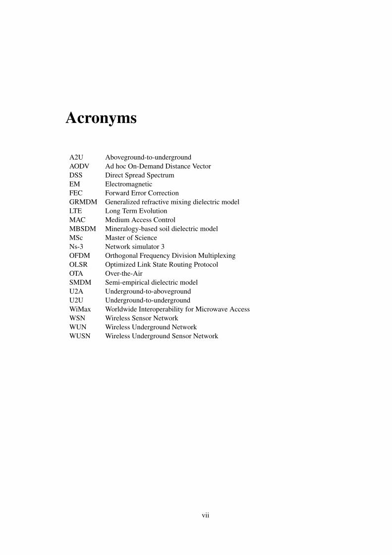
Acronyms

A2U Aboveground-to-undergroundAODV Ad hoc On-Demand Distance VectorDSS Direct Spread SpectrumEM ElectromagneticFEC Forward Error CorrectionGRMDM Generalized refractive mixing dielectric modelLTE Long Term EvolutionMAC Medium Access ControlMBSDM Mineralogy-based soil dielectric modelMSc Master of ScienceNs-3 Network simulator 3OFDM Orthogonal Frequency Division MultiplexingOLSR Optimized Link State Routing ProtocolOTA Over-the-AirSMDM Semi-empirical dielectric modelU2A Underground-to-abovegroundU2U Underground-to-undergroundWiMax Worldwide Interoperability for Microwave AccessWSN Wireless Sensor NetworkWUN Wireless Underground NetworkWUSN Wireless Underground Sensor Network

vii

Chapter 1

Introduction

1.1 Context

Underground communications are common in mines and tunnels. In the past years the research

work has been increasing in this area. Although these scenarios are different from the

aboveground over-the-air (OTA) communications, the propagation medium is still the air.

Wireless communications through soil with applications such as agriculture and maintenance of

playing fields are an emerging topic. Since this type of communications involve using the soil as

the propagation medium, new propagation models have to be created and new challenges have to

be addressed. The soil is characterized by several properties that we need to take into account,

such as texture and water content. In particular, the water content is a property that depends on

the weather and so it can vary from low water content in a sunny day to high water content in a

rainy day.

A wireless underground network typically includes underground and aboveground nodes, as

we can see in the Figure 1.1

Figure 1.1: Example of a wireless underground network with aboveground and undergroundnodes. [1]

Although there is significant research work produced in the last years, wireless underground

networks are an emerging topic and there are still many challenges and problems to be addressed.

1.2 Motivation

A number of research works have been made in the past few years regarding wireless underground

communications because they revealed to be a good alternative to wired solutions. However,

1

2 Introduction

the propagation medium is the soil, the communications properties vary from soil to soil, and

the amount of water also has significant influence in the propagation; for instance, the medium

characteristics will vary a lot with weather conditions.

In order to overcome the difficulties to design a network of this type we need to be able to

simulate the target network for several scenarios. Then, with the results we can determine, for

example, the minimum distance between nodes that can guarantee connectivity between nodes

for different amounts of water in the soil. Also, before doing field experiments, new wireless

underground networking solutions need to be evaluated in simulations, for the sake of easy control

of the tests. These difficulties in design a network are mainly due to the non-existence of simulators

for these scenarios.

The Ns-3 will be the simulator chosen for implement the simulation environment for

underground networks because it is widely used by the research community including our

research group. This implementation in a network simulator is an important step when designing

new networking solutions for this environment and also for research purposes.

1.3 Objectives

The goal of this dissertation is to develop a new simulation model for ns-3 that allows simulation

of wireless underground networks for different frequencies, types of soils and depths of the nodes.

The ns-3 model has to be able to simulate communications between buried nodes and between

buried nodes and aboveground nodes. To achieve this goal the work was divided into some specific

objectives:

• Study the major properties characterizing the soil and models;

• Study some experiments and the existing radio propagation models for underground

networks;

• Study the ns-3 simulation environment, in particular the methodology that shall be used to

implement and add new models to the simulator;

• Implement the propagation models in ns-3;

• Simulate the same experimental scenarios found in literature and compare the obtained

results with the documented ones;

• Conclude about the accuracy of the implemented wireless underground simulation

environment.

1.4 Document Structure

This document is organized in five chapters. Chapter 2 presents the state of the art in Wireless

Underground Networks (WUN) and the ns-3 network simulator. Chapter 3 shows the methodology

1.4 Document Structure 3

that will be used in order to achieve the goals described in this chapter. Chapter 4 describes the

work plan. Finally, Chapter 5 draws the major conclusions.

4 Introduction

Chapter 2

State of the art

In this chapter we present the state of the art on wireless underground networks. We start by

defining some concepts about these networks, and point out some recent applications. Then, we

present the major radio propagation models in underground networks, and also soil models for

estimate the soil dielectric constant. We also make an introduction to wireless networks in tunnels

and caves for the sake of completeness. Next, we present the ns-3 network simulator, since it will

be the simulator used as a basis to develop the simulation environment for WUNs, and we discuss

some important aspects of ns-3 in order to justify its use. Finally, we discuss the major topics

presented in this chapter.

2.1 Wireless Underground Networks

Wireless Underground Networks (WUN) are networks in which some or all the nodes are located

underground and use some wireless technology to communicate with each other. The

communication medium is the soil or hybrid (soil plus air) when some of the nodes are located

aboveground.

Since the medium in WUNs is different from the traditional wireless networks it requires the

definition of new propagation models, which have been proposed in the past few years. This type

of networks are mainly implemented with sensors that are monitoring some variable or process.

For this reason they are also called Wireless Underground Sensor Networks (WUSN) because

they are an extension of the traditional Wireless Sensor Networks (WSN). There are several

applications of WUSNs to improve some sort of monitoring [8]:

• Agriculture — sensors can be used to monitor the soil parameters, such as water content,

mineral content, salinity, and temperature, and then communicate these values in real time

to a control station aboveground, in order to have soil parameters in optimal values. This

type of monitoring can also be used in sports fields;

• Security — sensors buried at a shallow depth can detect movement at the surface. This is

useful for home security as well as military applications such as border patrol. Although

5

6 State of the art

this tasks can be done with aboveground sensors they benefit if they are underground since

in this case they remain hidden;

• Infrastructure Monitoring — a WUN can be used to monitor underground plumbing

leakage as well as electrical and communication wiring.

Figure 2.1: Example of WUN used in agriculture. [2]

Figure 2.2: Hybrid wireless sensor network for border patrol. [3]

Compared to wired underground networks, WUN has some advantages: they are easier to

deploy since the nodes don’t require a physical connection with each other and they are harder to

detect because there are no cables connecting the nodes.

2.2 Wireless Underground communication scenarios

In a wireless underground network there are buried nodes that communicate between them using

the soil as propagation medium, but there are also aboveground nodes communicating with

underground nodes; in the later case, the propagation medium is hybrid (the soil and the air).

Assuming bidirectional communication we will see that between a node aboveground and a node

underground the link aboveground-underground is different from the link

underground-aboveground and, for that reason we consider three different scenarios as we can

see in the figure 2.3:

• Underground-to-underground (U2U) — Communication between two nodes when both

of them are buried underground. In this scenario the propagation medium is always the soil.

This scenario is used in multi hop underground networks;

• Aboveground-to-underground (A2U) — Communication between an aboveground node

(the sender) and an underground node (the receiver). In this scenario the propagation

2.3 Underground channel models for WUNs 7

Figure 2.3: Types of communications in WUNs. [4]

medium is hybrid. This link is typically used to send control information to the

underground nodes;

• Underground-to-aboveground (U2A) — In this link the underground node is the sender

and the aboveground the receiver. The propagation medium is hybrid. This link is normally

used to send the data measured to the aboveground data station that behaves as a data sink.

2.3 Underground channel models for WUNs

In this section we present the propagation models for the three different links referred in Section

2.2. Since the soil is a very different medium compared to the air we also present models to

estimate its dielectric properties based on water content, percentage of sand and clay, and the

frequency used for transmission. In turn, these models are important to estimate the parameters of

the radio propagation models.

2.3.1 Dielectric soil properties model

In order to estimate the soil dielectric constant first we need to classify the kind of soil that we

are using, which can be done by collecting a sample of that soil and analyse it in a laboratory to

measure the percentage of sand, clay and silt. Based on these three parameters we can classify the

soil using the texture triangle that is presented in the Figure 2.4.

Besides these three parameters the soil also has an amount of water which can be expressed as

the Volumetric Water Content (VWC) that represents the fraction of water in the soil sample; as a

final input parameter for the dielectric model, we need the operating frequency.

In [9] the authors compare the semi-empirical mixing dielectric model (SMDM) proposed

by Dobson and the generalized refractive mixing dielectric model (GRMDM) in terms of their

precision for determining the soil dielectric constant of several types of soils, including types of

soils used to build the model and other types of soils. They conclude that the SMDM model is not

very accurate for types of soils other than those used to derive the model. The GRMDM prove to

be much more accurate in these tests, because it has the same accuracy to estimate the dielectric

constant of the soils used to build the model but specially because it has much more accuracy when

it comes to other soil types that are not the ones used to build the model.

8 State of the art

Figure 2.4: Soil texture triangle. [2]

The authors also present a model based on the GRMDM but with extra equations (Equation

2.9 to 2.17) to estimate some parameters that the GRMDM model requires to be measured. This

model, named mineralogy-based soil dielectric model (MBSDM), is described below and is the

one we selected to be our model to estimate the soil dielectric constant. The selection is based on

the simplicity of the SMDM model, which uses only the percentage of clay as input [9] and [10].

ε′ = n2

m− k2m (2.1)

ε′′ = 2nmkm (2.2)

According to this model the complex dielectric constant ε = ε ′+ jε ′′ can be calculated using

the Equations 2.1 and 2.2 respectively, where ε ′ is the dielectric constant and ε ′′ is the loss factor.

The parameters nm and km can be calculated as follows:

nm =

{nd +(nb−1)mv, if mv ≤ mvt

nd +(nb−1)mvt +(nu−1)(mv−mvt), if mv > mvt(2.3)

km =

{kd +(kb−1)mv, if mv ≤ mvt

kd +(kb−1)mvt +(ku−1)(mv−mvt), if mv > mvt(2.4)

The parameters nm, nd , nb, nu and km, kd , kb, ku are the values of the refractive index and

normalized attenuation coefficient. The subscripts m,d,b,u stand for moist soil, dry soil, bound

soil water and free soil water respectively. The rest of the n and k parameters can be calculated

using the following equations:

2.3 Underground channel models for WUNs 9

nd,b,u√

2 =

√√(ε ′d,b,u)

2 +(ε ′′d,b,u)2 + ε ′d,b,u (2.5)

kd,b,u√

2 =

√√(ε ′d,b,u)

2 +(ε ′′d,b,u)2− ε ′d,b,u (2.6)

The ε ′d,b,u are the real part of the dielectric constant of dry soil, bound water and free water

respectively. The imaginary part of the dielectric constants are expressed with the ε ′′d,b,u. This

model also present expressions for calculating the dielectric constant for bound water and free

water which are present next:

ε′b,u = ε∞ +

ε0b,0u− ε∞

1+(2π f τb,u)2 (2.7)

ε′′b,u =

ε0b,0u− ε∞

1+(2π f τb,u)2 (2π f τb,u)+σb,u

2πε0 f(2.8)

The f is the wave frequency, the values of σb,u, τb,u and ε0b,0u are the conductivities, relaxation

times and low frequency limit of dielectric constant for bound water and free water respectively.

The GRMDM model uses the equations present above from 2.1 to 2.8. With these equations we

can estimate the dielectric properties of the soil we are considering, but for doing that we need the

following soil parameters:

• Real (ε ′d) and Imaginary (ε ′′d ) parts of the complex dielectric constant for dry soil;

• Value of the maximum bound water fraction (mvt);

• Low frequency limits of dielectric constant for bound water (ε0b) and free water (ε0u);

• relaxation times for bound water (τ0b) and free water (τ0u);

• conductivities for bound water (σ0b) and free water (σ0u).

The value ε0 is the dielectric constant for free space and ε∞ is the high frequency limit which

is equal to 4.9 for bound and free water.

Now that the GRMDM model was presented and we conclude that we need a significant

number of parameters to use it, like the dielectric constant of the soil we are using without the

presence of water (dry soil) we conclude that the model is not very easy to use when compared

with the SMDM model proposed by Dobson, which requires only the sand and clay percentage of

the soil.

After the analysis of this model and its requirements we will present next some equations that

allow us to estimate the input parameters of the GRMDM model based only on the clay mass

percentage of the soil so that this model (named MBSDM) can be as easy to use as the SMDM

[9].

10 State of the art

nd = 1.634−0.539∗10−2C+0.2748∗10−4C2 (2.9)

kd = 0.03952−0.04038∗10−2C (2.10)

mvt = 0.02863+0.30673∗10−2 (2.11)

ε0b = 79.8−85.4∗10−2C+32.7∗10−4C2 (2.12)

τb = 1.062∗10−11 +3.450∗10−12 ∗10−2C (2.13)

σb = 0.3112+0.467∗10−2 (2.14)

σu = 0.3631+1.217∗10−2C (2.15)

ε0u = 100 (2.16)

τu = 0.5∗10−12 (2.17)

With the complex dielectric constant of the soil estimated we can determine the propagation

constant γ = α + jβ , where the α is the attenuation constant and β is the phase constant, using

Equations 2.18 and 2.19.

α = ω

√√√√√µε ′

2

√1+(

ε ′′

ε ′

)2

−1

, (2.18)

β = ω

√√√√√µε ′

2

√1+(

ε ′′

ε ′

)2

+1

(2.19)

2.3.2 Underground-to-underground propagation model

The characterization of the underground channel is very important for designing new WUSNs and

developing new protocols and mechanisms, such as new medium access control (MAC) optimized

for underground communications. Here we present some models to estimate the underground-to-

underground channel attenuation, which will then be used to create the ns-3 simulation model.

The simplest model is based on the Friis propagation model for free space and consists on

taking into account the attenuation based only on the distance between the nodes. The Friis

equation estimates the received signal strength at a distance d and can be written in the

logarithmic form as follows [11]:

Pr = Pt +Gr +Gt −L0 (2.20)

where Pt is the transmission power, Gr and Gt are the gains of the receiver and transmitter antennas,

respectively, and L0 is the path loss in free space which is given by

L0 = 32.4+20log(d)+20log( f ) (2.21)

2.3 Underground channel models for WUNs 11

where d is the distance between sender and receiver and f is the operation frequency in MHz. For

the propagation in soil we need to include a correction factor to take into account the soil medium,

which adds some extra attenuation. As result the received signal strength equation is written as

follow:

Pr = Pt +Gr +Gt − (L0 +Ls) (2.22)

where Ls is the additional path loss in the soil, calculated as follows:

Ls = Lβ +Lα = 154−20log( f )+20log(β )+8.69αd (2.23)

where β is the phase shifting constant and α the attenuation constant in soil.

The total path loss in dB for the direct propagation model can be expressed as follow:

PsldB = 6.4+20log(d)+20log(β )+8.69αd−10log(GaGb) (2.24)

Using Equation 2.24 we can get an approximation of the attenuation in dBs between a sender

and a receiver when both of them are buried. However, when estimating the total path loss in the

underground channel we need also to take into account the reflecting wave that result from the

underground surface, as shown in the Figure 2.5.

Figure 2.5: Two path channel model. [5]

This reflected wave has a greater effect when the buried depth of the nodes is lower, because in

this case the reflected ray has a reduced distance to travel. For this reason, this signal component

needs to be considered when estimating the path loss of the channel. The total path loss of the

channel considering the two-ray model can be computed using Equation 2.25 [5].

Pf ldB = PsldB−10log∣∣∣∣1+ √GcGdRdeα∆r√

GaGb(r1 + r2)e− j∆φ

∣∣∣∣2 (2.25)

Where Pf l is the 2-ray path loss, Gc and Gd is the antennas gain in the r1 and r2 directions,

respectively, ∆r = (r1 + r2)−d, ∆φ = 2π(r1 + r2−d)/λand R is the reflection coefficient of the

12 State of the art

soil-air interface and can be calculated as follow:

R =

1εr

cosθ −√

1εr− sin2(θ)

1εr

cosθ +√

1εr− sin2(θ)

(perpendicularly− polarixed) (2.26)

R =cosθ −

√1εr− sin2(θ)

cosθ +√

1εr− sin2(θ)

(parallel− polarized) (2.27)

As we can see from Equation 2.25 this new model take into account the buried depth of the

nodes.

2.3.3 Underground-to-aboveground propagation model

When building a WUSN we may also have aboveground nodes that can establish a bidirectional

communication with underground nodes. The aboveground nodes may act as data sinks and/or as

control stations. In this section we present a propagation model for the underground-aboveground

communications link.

As we can see in the Figure 2.6 this situation differs from the underground-to-underground

because now the propagated wave has to travel first in the soil, cross the soil-air interface, and then

propagate in the air.

Figure 2.6: Underground-to-aboveground channel model. [5]

According to [5] the path loss can be calculated with the following equation:

Pu−adB = PudB+PadB+10log∣∣∣∣ 1νe− j2π(d1/λ+d2/λ0

∣∣∣∣2Pu = 6+10log(d1)+20log(β )+8.69αd1−10log(Ga)

Pa = 20log( f )+20log(d2)−147.56−10log(Gb)

(2.28)

(2.29)

(2.30)

where ν is the refraction coefficient from soil to air given by:

2.3 Underground channel models for WUNs 13

ν =2cosθ1√

1εr

cos(θ1)+√

1− εrsin2(θ1)(perpendicularly− polarixed) (2.31)

ν =2cosθ1

cos(θ1)+√

1εr− sin2(θ1)

(parallel− polarized) (2.32)

As we can see in Equation 2.28 the path loss is a sum of three components where the first is

the attenuation in the soil medium, the second is the attenuation in the air medium, and the third

is the attenuation in the soil-air interface.

In the underground-aboveground path we need to be aware that the relative dielectric constant

of soil is greater than the air. So, if the incident angle (θ1) is larger than the critical angle (θc =

arcsin(√

1εr)) the ray will be completely reflected. In this case the refracted angle is approximately

90o so the signal will propagates along the ground surface.

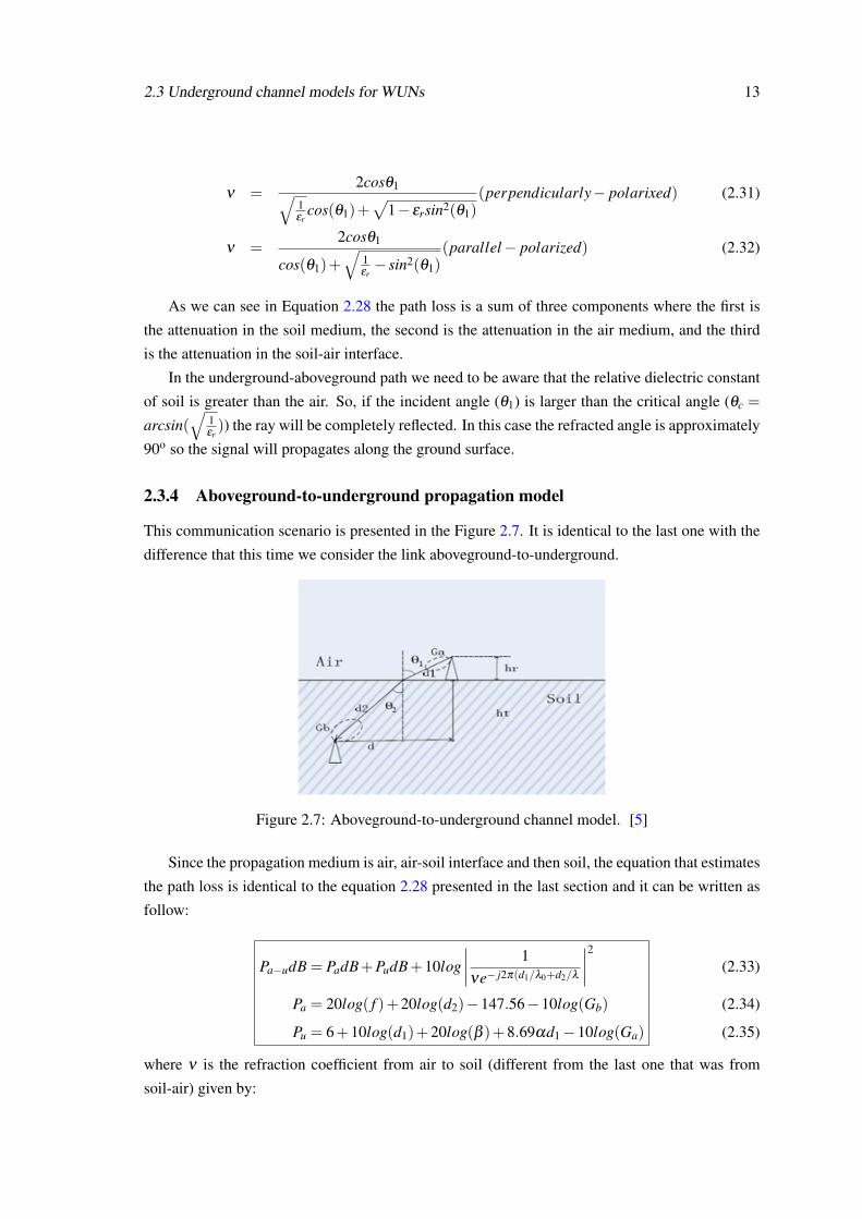
2.3.4 Aboveground-to-underground propagation model

This communication scenario is presented in the Figure 2.7. It is identical to the last one with the

difference that this time we consider the link aboveground-to-underground.

Figure 2.7: Aboveground-to-underground channel model. [5]

Since the propagation medium is air, air-soil interface and then soil, the equation that estimates

the path loss is identical to the equation 2.28 presented in the last section and it can be written as

follow:

Pa−udB = PadB+PudB+10log∣∣∣∣ 1νe− j2π(d1/λ0+d2/λ

∣∣∣∣2Pa = 20log( f )+20log(d2)−147.56−10log(Gb)

Pu = 6+10log(d1)+20log(β )+8.69αd1−10log(Ga)

(2.33)

(2.34)

(2.35)

where ν is the refraction coefficient from air to soil (different from the last one that was from

soil-air) given by:

14 State of the art

ν =2cosθ1√

1εr

cos(θ1)+√

1− εrsin2(θ1)(perpendicularly− polarixed) (2.36)

ν =2cosθ1

cos(θ1)+√

εr− sin2(θ1)(parallel− polarized) (2.37)

Now comparing Equations 2.33 and 2.28 we can see that they are basically identical. The only

difference is that in the U2A link the interface is soil-air, which means that the ray goes from a

higher refraction index to a lower refraction index; this leads to higher attenuation than in the A2U

scenario. In the U2A scenario total reflection can also occur, as we concluded in the early section.

2.4 Wireless Underground Networks in mines and tunnels

When analysing wireless underground communications scenarios we can have another scenario

which is the communication in a mine or a tunnel. In this case the communication medium is

always the air, but the propagation characteristics of the EM waves is very different from those of

the traditional aboveground communications, mostly due to the structure of the mine or the length

of the tunnel and the dielectric properties of the walls.

There are also several mathematical models to describe this scenario and one of them is present

in [1] and is named Multimode Model. This model is capable of characterizing completely the

wave propagation on a tunnel in both near and far regions. However when we are dealing with

caves the scenario can be different because in this case we need to consider the pillars that are

disposed randomly. The multimode model overcomes this problem by combining their results with

the shadow fading model in order to estimate the effects of reflections and diffractions suffered by

the signal.

These networks have been the focus of many researches and are considered underground

networks yet, since the medium is only the air they are out of scope for this MSc work.

2.5 Ns-3 Simulator

Ns-3, network simulator three, is an open-source discrete event network simulator targeted

primarily for research and education purposes. It was written using the c++ programming

language but the ns-3 library is wrapped to python thanks to the pybindgen library so if some

users feels more comfortable with python they can use it instead of c++ to interact with the

libraries.

The ns-3 is split into a couple dozens of modules and each implement one or more models for

real world network devices and protocols such as Wi-fi, WiMax, LTE for layers one and two and

also several routing protocols such as OLSR and AODV.

When compared to other network simulators the ns-3 has some distinguishing high level design

goals such as [12]

2.6 Summary 15

• C++ and Python emphasis — instead of use a domain specific modelling language to

describe the models ns-3 uses the c++ or python languages;

• Callback-driven events and connections — simulation events in ns-3 are simply function

calls that are scheduled to execute at a prescribed simulation time by use of a callback

function as in contrast to specialized "handler" functions that centralize the processing of

events in each simulation object;

• Flexible core with helper layer — ns-3 has a low level API that gives the users a lot of

flexibility to configure the objects. However it also has some helper classes with some

default configurations and easier to use functions;

• Alignment with real-world interfaces — ns-3 nodes, interfaces and objects such us

sockets and net devices are aligned with those found in a Linux computer which improves

the realism of the models and makes the comparison with real systems easier.

Since ns-3 is an open-source simulator and is widely spread over the research community and

due to the lack of simulation models for underground communications these will be implemented

and tested in this simulator during the realization of this MSc dissertation.

2.6 Summary

In this chapter we started by analysing some of the applications for WUNs and defined the

communication scenarios that will be the targeted in this MSc work. Then, we presented some

mathematical models for describing the soil properties and propagation characteristics in each of

the three communication scenarios that will be simulated. For the propagation characteristics the

main equations that are important to notice are: Equation 2.25 for the U2U scenario; Equation

2.28 for the U2A link; and Equation 2.33 for the A2U link. For concluding the state of the art in

wireless underground networks we also referred wireless networks in tunnels and mines because

although they are beyond the dissertation objectives they still belong to the WUN group.

Since the main objective of this work is to implement the theoretical models into the ns-3

simulator we also went through an explanation of ns-3 and why we have chosen it. It is also

important to notice that there is no simulation tool for these networks yet.

16 State of the art

Chapter 3

Methodology

After identifying the main goal of the dissertation, which is to create a ns-3 accurate model capable

of simulating wireless underground networks, and studying theoretical models for predicting the

soil dielectric constant and signal attenuation, in this chapter we define the strategy that will be

used to create the ns-3 model and validate it with experimental results. This chapter presents the

methodology that will be followed during the development of this dissertation.

3.1 Ns-3 propagation model details

The simulation model that will be implemented should be able to predict the signal attenuation, the

delay and the packet error ratio between two nodes in the cases of one or two buried nodes. Since

the dielectric constant of the soil vary from one soil to another, based on the soil properties and

volumetric water content, we identify another requirement for the model, which is, to estimate the

complex soil dielectric constant based on the physical soil properties and the operating frequency

of the connection nodes.

The class ns3::TwoRayUndergroundModel will be created in ns-3 to implement our model. In

Figure 3.1 we can see the ns-3 architecture and the layer where our model will be focused which

is the propagation layer.

Figure 3.1: Ns-3 Architecture. [6]

For estimating the signal attenuation we will use the mathematical equations presented in

Chapter 2. The important equations for the underground channel that will be the used are:

Equation 2.25 for the U2U communication, Equation 2.28 for the U2A link and, Equation 2.33

for the A2U link.

17

18 Methodology

For the delay calculation we will use one of the already implemented models which is the

ns3::ConstantSpeedPropagationDelayModel that considers the delay constant along the path

between the sender and the receiver. It is important to notice that this is true if we are only

considering the U2U link, since in this case the electromagnetic wave will propagate exclusively

in the soil. When we are considering one node aboveground there will be two propagation

mediums. In this case we will use two instances of this model, one for the signal component that

travels in the soil and another for the signal component that travels over the air; then we sum the

two delays and have the total delay between the two nodes.

Another important property that is interesting to estimate when we are designing a new

communication scenario is the packet error ratio, because above a threshold it is no longer

possible to establish communication between the nodes. The error ratio has dependencies not

only with the power receiver sensitivity but also with the frequency used, the modulation

techniques (OFDM, DSS) and with the forward error correction (FEC) codes used (if any). In

order to be able to take these variables into account we will use the already implemented

ns3::NistErrorRateModel for the cases where we use the OFDM technique and the

ns3::DssErrorRateModel for the cases where we use the DSS.

Another important property that needs to be estimated is the complex dielectric constant,

which is evaluated using the soil physical properties and the amount of water. In Chapter 2 we

presented two mathematical models to calculate the dielectric constant, which are the SMDM

model and the MBSDM model. With some analysis between experimental and theoretical results

found in literature we concluded that the MBSDM model is more accurate and so we focus on

this model and implement it in ns-3. However, due to the simplicity of adding another dielectric

model to our implementation, and since the SMDM model is widely spread in literature, we will

also include this model. By adding more than one mathematical model we give the user a chance

to choose which model he wants to use to compute the dielectric constant. During our

investigation on previous experiments with these networks, with the objective of validating our

model, we also found very common in these experiments the presence of the values for the

dielectric constant instead of the physical soil properties. So, we decided to give another option

for this constant which is the user be able to introduce it directly in our ns-3 model instead of

estimate it with one of the two models described above. Besides the dielectric constant values we

also find common to only characterize the soil using the terms in Figure 2.4, and, consequently

we decided to include a table with several soil types like, for example, sandy or loam and their

approximate dielectric constant. This table is a great help in obtain preliminary results before

making an analysis to a soil sample.

3.2 Simulation scenarios

After the implementation of the ns-3 propagation model presented in the Section 3.1 is completed

we will validate the model by simulating the scenarios presented in the state of the art (U2U,

A2U and U2A) for several soil types and different water content, frequencies, depths of the buried

3.3 Summary 19

nodes, lateral distance, and heights of the aboveground nodes. The simulations will be done

using the 802.11 MAC, already implemented in ns-3, and the networks will be tested in both

infrastructure and ad-hoc modes.

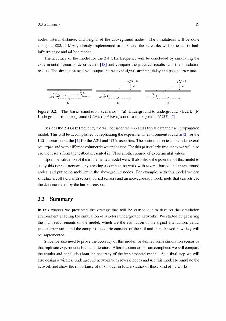
The accuracy of the model for the 2.4 GHz frequency will be concluded by simulating the

experimental scenarios described in [13] and compare the practical results with the simulation

results. The simulation tests will output the received signal strength, delay and packet error rate.

Figure 3.2: The basic simulation scenarios: (a) Underground-to-underground (U2U), (b)Underground-to-aboveground (U2A), (c) Aboveground-to-underground (A2U). [7]

Besides the 2.4 GHz frequency we will consider the 433 MHz to validate the ns-3 propagation

model. This will be accomplished by replicating the experimental environment found in [2] for the

U2U scenario and the [4] for the A2U and U2A scenarios. These simulation tests include several

soil types and with different volumetric water content. For this particularly frequency we will also

use the results from the testbed presented in [7] as another source of experimental values.

Upon the validation of the implemented model we will also show the potential of this model to

study this type of networks by creating a complex network with several buried and aboveground

nodes, and put some mobility in the aboveground nodes. For example, with this model we can

simulate a golf field with several buried sensors and an aboveground mobile node that can retrieve

the data measured by the buried sensors.

3.3 Summary

In this chapter we presented the strategy that will be carried out to develop the simulation

environment enabling the simulation of wireless underground networks. We started by gathering

the main requirements of the model, which are the estimation of the signal attenuation, delay,

packet error ratio, and the complex dielectric constant of the soil and then showed how they will

be implemented.

Since we also need to prove the accuracy of this model we defined some simulation scenarios

that replicate experiments found in literature. After the simulations are completed we will compare

the results and conclude about the accuracy of the implemented model. As a final step we will

also design a wireless underground network with several nodes and use this model to simulate the

network and show the importance of this model in future studies of these kind of networks.

20 Methodology

Chapter 4

Workplan

In this chapter we present the workplan that will be carried out during the development of this

dissertation. This plan is presented in figure 4.1 in a form of Gantt diagram and it presents the

main activities that need to be done in order for us to accomplish the dissertation goals established

in the first chapter.

• 10/02 - 18/02 - Define all the details in order to implement the ns-3 model;

• 19/02 - 01/04 - Implement the underground simulation environment in ns-3;

• 02/04 - 18/04 - Implement the experimental scenarios and simulate them;

• 21/04 - 02/05 - Conclude about the accuracy of the model based on the obtained results and

adjust model parameters;

• 05/05 - 23/05 - Simulate a complex network to study their behaviour with our simulator;

• 26/05 - 27/06 - Write the final report.

Figure 4.1: The workplan for this dissertation.

In this diagram it is possible to see the order in which the activities will be carried out and also

the start and finish dates of each one and consequently their estimated duration in days.

21

22 Workplan

Chapter 5

Conclusion

This dissertation arises in the context of establish wireless networks in the underground

environment. The goal is to develop an accurate simulation framework for this kind of networks,

which will be implemented over the ns-3 simulator.

Upon the review of the state of the art we have found several challenges in wireless

underground communications. These challenges are mainly due to the fact that the EM waves

propagates differently in the soil when compared to the over the air communications. The

propagation parameters also vary from one soil type to another or even in the same soil if we

have different amounts of water, which is dependent on weather conditions. These difficulties

together with the fact that there are no simulation tools available for WUNs, upon the writing of

this document, makes the design of wireless underground networks difficult.

After the characterization of the main objectives of the dissertation and reviewing the state of

the art, we presented in Chapter 3 the strategy that will be used to implement the simulation model

in ns-3 and to validate it by simulating some underground communications found in literature.

After this validation is completed we will also design a complex network and demonstrate the

power of this framework to study and design this type of networks.

23

24 Conclusion

References

[1] Ian F. Akyildiz, Zhi Sun, and Mehmet C. Vuran. Signal Propagation Techniques for WirelessUnderground Communication Networks. Physical Communication, 2(3):167–183, 2009.

[2] Agnelo R. Silva. Channel Characterization for Wireless Underground Sensor Networks.Thesis, 2010.

[3] Mehmet C. Vuran c Mznah A. Al-Rodhaan b Zhi Sun, Pu Wanga and Ian F. AkyildizAbdullah M. Al-Dhelaan b. BorderSense: Border Patrol Through Advanced Wireless SensorNetworks. Elsevier, page 468–477, 2011.

[4] A.R. Silva Vuran. and M.C. Communication with Aboveground Devices in WirelessUnderground Sensor Networks: An Empirical Study, 2010.

[5] Hu Xiaoya, Gao Chao, Wang Bingwen, and Xiong Wei. Channel Modeling forWireless Underground Sensor Networks. 2012 IEEE 36th Annual Computer Software andApplications Conference Workshops, pages 249–254, 2011.

[6] Ns-3 Manual.

[7] Agnelo R. Silva Vuran and Mehmet C. Development of a Testbed for Wireless UndergroundSensor Networks. EURASIP Journal onWireless Communications and Networking, page 14,2009.

[8] D. Pompili E.P. Stuntebeck and T. Melodia. Wireless Underground Sensor Networks UsingCommodity Terrestrial Motes, 2006.

[9] Lyudmila G. Kosolapova Valery L. Mironov and Sergej V. Fomin. Physicallyand Mineralogically Based Spectroscopic Dielectric Model for Moist Soils. IEEETRANSACTIONS ON GEOSCIENCE AND REMOTE SENSING, 47:2059 –2070, 2009.

[10] Lyudmila G. Kosolapova Valery L. Mironov and Sergej V. Fomin. Correction to “Physicallyand Mineralogically Based Spectroscopic Dielectric Model for Moist Soils”. IEEETRANSACTIONS ON GEOSCIENCE AND REMOTE SENSING, 47:2085, 2009.

[11] Mehmet C. Vuran and Ian F. Akyildiz. Channel Model and Analysis for WirelessUnderground Sensor Networks in Soil Medium. Physical Communication, 3(4):245–254,2010.

[12] ns-3. http://www.nsnam.org/, November 2013.

[13] José Oliveira. Wifi Underground Wireless Networks. Thesis, 2013.

25