npl report eng 32 an overview of industrial x-ray computed
TRANSCRIPT

NPL REPORT ENG 32 An overview of industrial X-ray computed tomography Sun W, Brown S B and Leach R K JANUARY 2012


NPL Report ENG 32
i
An overview of industrial X-ray computed tomography
Sun W, Brown S B and Leach R K Engineering Measurement Division
ABSTRACT Driven by the need for quality control of complex three-dimensional engineering components, and enabled by progress in medical imaging and consumer graphics processing, X-ray computed tomography (XCT) has been increasingly used for industrial inspection in recent years. A review of the recent development of industrial XCT systems in the context of traceable dimensional metrology is presented. The market trends of industrial XCT systems are briefly reviewed. Progress towards standards and methods for XCT calibration and verification are studied in detail. The report also covers the recent development of both hardware and software and discusses the challenges regarding systematic errors. Commercial systems are summarised to establish the capability available to the industrial user. Finally, what will be required to develop XCT technology in the field of dimensional metrology is considered.

NPL Report ENG 32
ii
Queen’s Printer and Controller of HMSO, 2012
ISSN 1754-2987
National Physical Laboratory Hampton Road, Teddington, Middlesex, TW11 0LW
Extracts from this report may be reproduced provided the source is acknowledged and the extract is not taken out of context.
Approved on behalf of NPLML by Dr A J Lewis, Assistant Knowledge Leader.
NPL Report ENG 32
iii
CONTENTS
1 INTRODUCTION ......................................................................................................................... 1
1.1 THE X-RAY SPECTRUM AND XCT SYSTEMS .............................................................................. 2 1.2 CLASSIFICATION OF INDUSTRIAL XCT SYSTEMS ...................................................................... 3 1.3 ADVANTAGES OF XCT .............................................................................................................. 4 1.4 ANALYSIS AND INSPECTION ..................................................................................................... 5
2 INDUSTRIAL OVERVIEW ........................................................................................................ 6
2.1 CURRENT INDUSTRIAL TRENDS ................................................................................................ 6 2.2 EMERGING MARKETS ............................................................................................................... 7
2.2.1 Food inspection ............................................................................................................... 7 2.2.2 Security ............................................................................................................................ 7 2.2.3 Microelectronics .............................................................................................................. 7
2.3 FUTURE MARKETS .................................................................................................................... 7 2.3.1 New material technologies .............................................................................................. 7 2.3.2 Military hardware ........................................................................................................... 7 2.3.3 Infrastructure ................................................................................................................... 8 2.3.4 Industrial versus medical systems ................................................................................... 8 2.3.5 Aerospace demands ......................................................................................................... 8 2.3.6 Electronics demands ........................................................................................................ 9
3 XCT HARDWARE ..................................................................................................................... 10
3.1 X-RAY SOURCE ...................................................................................................................... 10 3.2 X-RAY DETECTORS ................................................................................................................. 12 3.3 PROPERTIES OF XCT DETECTORS ............................................................................................ 14 3.4 PC HARDWARE ....................................................................................................................... 16 3.5 SHIELDING ............................................................................................................................. 17 3.6 COOLING SYSTEM................................................................................................................... 17
4 DATA PROCESSING ................................................................................................................. 18
4.1 RECONSTRUCTION OF CONE-BEAM XCT ................................................................................. 20 4.2 COMMERCIAL VISUALISATION SOFTWARE PACKAGES........................................................... 22 4.3 FREEWARE ............................................................................................................................. 22
5 SYSTEMATIC ERRORS IN XCT ............................................................................................ 24
5.1 BEAM DRIFT ........................................................................................................................... 24 5.2 RING ARTEFACTS ................................................................................................................... 24 5.3 BEAM HARDENING ................................................................................................................. 26 5.4 PARTIAL VOLUME ARTEFACTS ............................................................................................... 28 5.5 OTHER SYSTEMATIC ERRORS ................................................................................................. 29
6 XCT SYSTEM CALIBRATION AND VERIFICATION ....................................................... 30
6.1 XCT SYSTEM CALIBRATION .................................................................................................... 30 6.2 XCT SYSTEM VERIFICATION ................................................................................................... 31 6.3 INTERNATIONAL STANDARDS FOR XCT TECHNOLOGY .......................................................... 31 6.4 SYSTEM CAPABILITIES ........................................................................................................... 32
6.4.1 Spatial resolution .......................................................................................................... 33 6.4.2 Artefacts......................................................................................................................... 33 6.4.3 Statistical noise .............................................................................................................. 34
6.5 REFERENCE OBJECTS .............................................................................................................. 34 6.5.1 PTB ................................................................................................................................ 34 6.5.2 Zeiss ............................................................................................................................... 35 6.5.3 International comparison of micro-CMM and XCT systems ......................................... 36

NPL Report ENG 32
iv
6.5.4 CT Audit comparison ..................................................................................................... 36 6.5.5 Other reference objects ................................................................................................. 38
6.6 DESIGN OF REFERENCE STANDARDS ...................................................................................... 40
7 COMMERCIALLY AVAILABE INDUSTRIAL XCT SYSTEMS ....................................... 42
7.1 CARL ZEISS AG ....................................................................................................................... 43 7.2 GE SENSING & INSPECTION TECHNOLGIES ............................................................................. 43 7.3 NIKON METROLOGY NV .......................................................................................................... 44 7.4 NORDSON CORPORATION ....................................................................................................... 44 7.5 SKYSCAN ................................................................................................................................ 45 7.6 NORTH STAR IMAGING INC. .................................................................................................... 45 7.7 WERTH MESSTECHINK GMBH ................................................................................................. 46 7.8 XRADIA .................................................................................................................................. 46 7.9 UK INSTITUTIONS AND XCT RELATED WORK ......................................................................... 47
8 CONCLUSIONS .......................................................................................................................... 48

NPL Report ENG 32
v
FIGURES
Figure 1. The electromagnetic spectrum [4] ........................................................................ 2 Figure 2. Structure of XCT systems .................................................................................... 2 Figure 3. A line beam scanner ............................................................................................. 3 Figure 4. A typical cone beam scanner ............................................................................... 4 Figure 5. XCT reconstruction, from [6] .............................................................................. 5 Figure 6. Typical output plot from commercial software showing a colour map of
deviation of measured point cloud data positions from that predicted by the CAD
drawing ........................................................................................................................ 5 Figure 7. Imaging trends: diagnostic imaging procedure volume by modality [8] ............. 8 Figure 8. X-ray spectrum................................................................................................... 11 Figure 9. Transmission and reflection X-ray production .................................................. 11 Figure 10. Advances in detector technology [28] ............................................................. 13 Figure 11. Direct detection of X-ray photons .................................................................... 13 Figure 12. Structure of a scintillation detector [28] .......................................................... 14 Figure 13. XCT cubic matrix of attenuation coefficients .................................................. 18 Figure 14. Illustration of Radon transform for a square object (top) image of a square
(bottom) Radon transform of the square image from 0 to 180 ............................... 19 Figure 15. Inverse of Radon transform (left) original square image (middle) image
reconstructed using filtered backprojection process (right) image calculated using
unfiltered backprojection process .............................................................................. 19 Figure 16. Operation of typical filters [46] ....................................................................... 20 Figure 17. Structure of a reflection type X-ray tube ......................................................... 24 Figure 18. Illustration of ring artefacts (courtesy Nikon Metrology) ................................ 25 Figure 19. Image of ring artefact removed (courtesy Nikon Metrology) .......................... 25 Figure 20. Illustration of X-ray penetrating sample with different thickness [78] ............ 26 Figure 21. Beam hardening effects (left) an image without filtering (right) an image
with a 1 mm thick copper filter (courtesy Nikon Metrology) ................................... 27 Figure 22. Illustration of ring artefacts and streak artefacts .............................................. 27 Figure 23. Cupping due to beam hardening ...................................................................... 28 Figure 24. Illustration of partial volume artefacts [67], images of three 12 mm
diameter acrylic rods supported in air parallel to and approximately 15 cm from
the scanner axis, (left) image obtained with the rods partially intruded into the
section width, showing partial volume artefacts, (right) image obtained with the
rods fully intruded into the section width, showing no partial volume artefacts ....... 29 Figure 25. Example test procedure for obtaining the MTF [115] ..................................... 33 Figure 26. Reference objects developed by PTB [131, 132] ............................................. 34 Figure 27. Cast part developed by ACTech GmbH [133] (left) work-piece-near
reference object on holding plate (right) two of the four segments of the reference
object ......................................................................................................................... 35 Figure 28. Zeiss calibration reference sphere [134] .......................................................... 35 Figure 29. 4 mm diameter sphere ...................................................................................... 36 Figure 30. 1 mm diameter sphere ...................................................................................... 36 Figure 31. Tetrahedral group of 0.5 mm spheres .............................................................. 36 Figure 32. CT Audit items [136] ....................................................................................... 37 Figure 33. Reference objects developed by Carmignato et al [138] ................................. 38 Figure 34. Determining the threshold value [138] ............................................................ 39 Figure 35. The aluminium cactus block [139] (left) front view (right) 3D model of the
sample ........................................................................................................................ 39 Figure 36. CAD model of workpiece [140]....................................................................... 39

NPL Report ENG 32
vi
TABLES Table 1. XCT classification ................................................................................................. 4 Table 2. Comparison of reconstruction algorithms [48] ................................................... 21 Table 3. Examples of error sources in 3D XCT measurements ........................................ 30 Table 4 XCT related international standards ..................................................................... 32 Table 5. Manufacturers of industrial XCT systems ........................................................... 42 Table 6. Summary of Carl Zeiss XCT systems ................................................................. 43 Table 7. Summary of GE XCT systems ............................................................................ 43 Table 8. Summary of Nikon XCT systems ....................................................................... 44 Table 9. Summary of Nordson Dage XCT systems .......................................................... 44 Table 10. Summary of Skyscan XCT systems .................................................................. 45 Table 11. Summary of North Star Imaging XCT systems ................................................ 46 Table 12. Summary of Werth Messtechnik XCT systems ................................................ 46 Table 13. Summary of Xradia XCT systems..................................................................... 47 Table 14. Summary of UK universities that with XCT systems ....................................... 47

NPL Report ENG 32
1
1 INTRODUCTION
X-ray computed tomography, abbreviated as XCT or CT, uses X-rays to take multiple two
dimensional (2D) transmission images of an object from different orientations. These images
are then processed, using computers, to construct a three dimensional (3D) image of the
object, including its interior geometry. The word ‘tomography’ is derived from two Greek
words, ‘tomos’ meaning ‘slice’ — images are taken through the volume of the object — and
‘graphein’ meaning ‘to write’ or record the image.
The idea that the inside structure of an object could be determined from multiple X-ray
images and from various angles around that object was developed by Godfrey Hounsfield
while working for EMI in the UK [1]. Hounsfield was not aware that, at the same time he was
developing his system, Allan Cormack from Tufts University in the USA was working on the
theory for such a device. In 1979, Hounsfield and Cormack were awarded the Nobel Prize for
Physiology or Medicine, in recognition of the development of XCT. The ‘Hounsfield’ was
subsequently introduced in the medical field as a unit for the measurement of radiodensity, or
the absorption of X-rays as they pass through a given material [2]. The Hounsfield is given
the symbol HU and is defined such that the radiodensity of distilled water at standard
temperature and pressure (STP) is equal to zero Hounsfield units (HU), while the radiodensity
of air at STP is equal to -1000 HU. On this scale, compact bone has a value of +1000 HU.
XCT systems have been in existence since the 1970s and were first used in medical imaging
to supplement 2D X-ray images (also known as radiographs) and ultrasound. Although XCT
and magnetic resonance imaging (MRI) techniques are similar, in that both employ
electromagnetic radiation, they differ in that XCT uses ionizing radiation whereas MRI uses
non-ionizing radiation, for example radio frequency radiation. XCT relies on absorption of X-
rays, whereas MRI uses the magnetic resonance of hydrogen molecules. Consequently, both
techniques have different areas of application. XCT is a useful tool for examining compounds
of elements with high atomic number whereas MRI is used in examining soft animal tissue.
In the area generally referred to as medical XCT, systems can be used as full body scanners or
in the targeted investigation of parts of the body, head, lungs, heart, etc. Although there are
many advantages from the use of XCT systems, there is also the disadvantage that exposure
to radiation may cause cancers. It is reported [3] that, in the United States in 2007, seventy-
two million scans were carried out and that 0.4 % of current cancers are due to XCT scans
preformed in the past, with this figure rising to as high as 1.5 % to 2 % with the current rate of
XCT scans. Knowing, through calibration, the correct dosage to apply will help dramatically
reduce the risk of initiating cancers.
Another area of use for XCT is classed as ‘industrial XCT scanning’ where it is used in the
detection of material flaws such as voids, cracks and for dimensional measurements. With
advances in software, the capability of XCT as a metrology tool has grown to allow
measurements of the internal and external geometry of complex parts. Prior to the use of XCT
systems, to measure internal dimensions, companies relied on either disassembly or
destructive testing of the object. XCT systems can measure these objects and verify that they
conform to the original design specification.
This report is a review of the application of XCT as a measuring tool for industrial
applications. This review will highlight trends, from current and emerging markets and areas
where XCT systems are used as a metrology tool. The review will highlight the need for
traceability of XCT systems, including some current work in this field. An overview of the
hardware and software that make up XCT systems is included. Some known errors, random
and systematic, will be discussed. An overview of some of the XCT systems that are currently
available on the market will be listed. The review will finally draw a conclusion to its findings
and highlight areas that it deems need further research work.
NPL Report ENG 32
2
1.1 THE X-RAY SPECTRUM AND XCT SYSTEMS
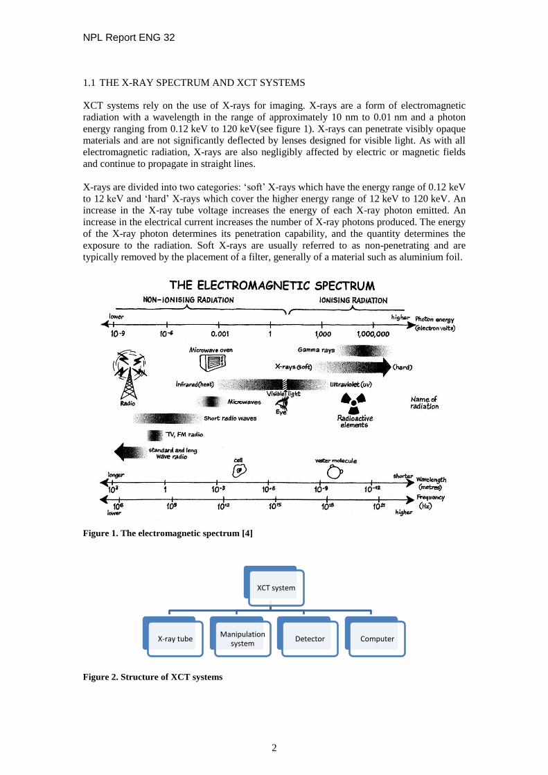
XCT systems rely on the use of X-rays for imaging. X-rays are a form of electromagnetic
radiation with a wavelength in the range of approximately 10 nm to 0.01 nm and a photon
energy ranging from 0.12 keV to 120 keV(see figure 1). X-rays can penetrate visibly opaque
materials and are not significantly deflected by lenses designed for visible light. As with all
electromagnetic radiation, X-rays are also negligibly affected by electric or magnetic fields
and continue to propagate in straight lines.
X-rays are divided into two categories: ‘soft’ X-rays which have the energy range of 0.12 keV
to 12 keV and ‘hard’ X-rays which cover the higher energy range of 12 keV to 120 keV. An
increase in the X-ray tube voltage increases the energy of each X-ray photon emitted. An
increase in the electrical current increases the number of X-ray photons produced. The energy
of the X-ray photon determines its penetration capability, and the quantity determines the
exposure to the radiation. Soft X-rays are usually referred to as non-penetrating and are
typically removed by the placement of a filter, generally of a material such as aluminium foil.
Figure 1. The electromagnetic spectrum [4]
Figure 2. Structure of XCT systems
XCT system
X-ray tube Manipulation
system Detector Computer

NPL Report ENG 32
3
An XCT system usually consists of an X-ray source, a sample manipulation system, a
radiation detector and a computer system to analyse data. Figure 2 shows the structure of
XCT systems. In operation, an X-ray tube emits an X-ray beam. The detector collects
projection images of the sample from different angles when either the sample or the X-ray
source and the detector rotate. The data can then be analysed in a computer and the image of
the sample under test reconstructed.
1.2 CLASSIFICATION OF INDUSTRIAL XCT SYSTEMS
According to the shape of the X-ray beam, industrial XCT systems on the market can be
divided into fan/line beam scanners and cone beam scanners, and then subdivided into their
energy range.
Fan/line beam scanners
Fan/line beam scanners were the first generation X-ray scanners and employ the use of a
beam of X-rays to scan through the volume of the object as it is rotated (see figure 3). All of
the resulting 2D slices are then used to construct a 3D representation of the object. Fan beam
tomography (2D tomography) tends to use linear X-ray detectors.
Figure 3. A line beam scanner
Cone beam scanners
Cone beam scanners use a cone beam of X-rays (see figure 4), to take over a thousand images
of the object as it is rotated around a fixed axis. These 2D images are then processed to create
a 3D reconstruction of the object (see section 4.1). These scanners tend to use 2D flat panel
X-ray detectors. In most cases the projected beam passes through the object and onto a
detector. The reconstruction method is usually based on the Feldkamp algorithm (FDK) [5].
Information on image reconstruction is discussed in section 4.1.

NPL Report ENG 32
4
Figure 4. A typical cone beam scanner
Energy range
There are generally four energy levels for XCT systems, which are commonly grouped by
their source energy (here energy is expressed in units of electron-volts) and these are
summarised in table 1. For an overview of resolution, please refer to sections 3.3 and 6.4.1.
Table 1. XCT classification
Type Energy range Resolution
Nano n/a < 1 µm
Low-power 0 to –110 keV > 1 µm
Mid-power 110 keV to –999 keV > 1 µm
High-power > 1 MeV > 1 µm
1.3 ADVANTAGES OF XCT
XCT systems are beginning to surpass conventional tactile co-ordinate measuring machines
(CMMs) or laser scanners in some areas due to advantages that are listed below:
capability for non-destructive-testing (NDT) for inspection and metrology;
significant reduction of inspection and analysis costs from first article to production;
ability to quickly and accurately validate design requirements for both internal and
external components;
precision measurement of complex internal features without destructive testing;
fixture requirements - parts are scanned in a free-standing state, minimising risk of
damage or clamping deformation errors;
ability to reverse engineer enclosed geometries and components; and
reduction in development costs in creating the first CAD model.

NPL Report ENG 32
5
1.4 ANALYSIS AND INSPECTION
XCT systems generate volumetric images from 2D images of the object under investigation
where these image stacks are individually referred to as radiographs (see figure 5). By
reconstructing the image stacks (see section 4) the volumetric image is constructed. A voxel is
a unit of graphical information that defines a point in a 3D space. In the case of an XCT scan,
a voxel also has a value that represents the density of the material at the point represented by
the voxel.
Figure 5. XCT reconstruction, from [6]
Measurements can be performed on individual parts or the assembly of parts, with
comparisons easily made with the original design drawings (CAD models). Colour-coded
deviation plots (see an example in figure 6) facilitate rapid visual inspection of the object,
often saving time and cost. One of the advantages of XCT over alternative inspection
techniques is the fact that failed objects (for example a pump) can be scanned in their failed
state without the need to disassemble the part - disassembly might cause further failures that
could disguise the initial problem.
Figure 6. Typical output plot from commercial software showing a colour map of deviation of
measured point cloud data positions from that predicted by the CAD drawing

NPL Report ENG 32
6
2 INDUSTRIAL OVERVIEW
As awareness of the benefits of XCT systems has increased, and additional distinct user
applications identified, the demand for higher resolution and more accurate measurements has
become apparent. This increase in the applications of XCT systems has initiated research into
the worldwide markets for XCT scanners (see for example, [7]).
In its infancy XCT was a diagnostic tool, generally used in medical applications for the
investigation of tumours in the human body. Today, there are film-based X-ray inspection
systems, XCT inspection systems and computed radiography inspection systems. The market
for such systems is growing and includes industries such as aerospace and defence,
automotive, and energy and electronics. Sales of XCT systems were affected during the 2008
to 2009 peak of the current global financial crisis, but are recovering. It is estimated that the
world market earned revenues for X-ray inspection systems in 2009 was $344 million and it is
predicted that this will grow to $450 million in 2014 [8]. It is estimated that global
installations of XCT scanners will reach 60 000 units by 2015 [9]. Industrial requirements can
be subdivided into three trends, which will be discussed in section 2.1.
A survey produced by Frost & Sullivan [8], states that of the total X-ray inspection system
market, the percentage of revenues by geographical region in 2009 was 32.2 % from North
America, 27.5 % from Europe, 27.3 % from Asia Pacific and the remaining 13 % from the
rest of the world.
The entire application of XCT for NDT has been enabled by medical funding and R&D as
well as consumer camera and graphics cards development. The XCT NDT development path
has been limited by progress in these industries.
2.1 CURRENT INDUSTRIAL TRENDS
Requirements for quality and safety have led the aerospace industry to maintain its position as
the largest user of X-ray inspection systems through its use in NDT. However, disasters in the
oil industry, such as that in the Gulf of Mexico, have led the oil and gas industry to have a
more critical approach to the maintenance of its equipment. The oil and gas industry is also a
user of XCT for on-site and field inspection, to estimate the viability of oil extraction.
Emerging from the economic crisis, the automotive industry is also placing greater emphasis
on improving the overall productivity and efficiency of manufacturing operations.
The digital age has had a crucial influence on the capture and analysis side of X-ray
inspection techniques. Digital cameras have made the capture of images easier, the use of
computers to analyse these images has made diagnostics more repeatable and the ability to
generate 3D images has given the operator a different view on the data. Software packages
have sufficiently simplified the acquisition and analysis of the images that these systems can
now be operated by a non-specialist.
The profound economic, human and environmental impact of recent industrial disasters, such
as the 2011 Fukushima nuclear plant incident in Japan, the 2010 BP fire and oil spill in the
Gulf of Mexico, the 1984 Bhopal tragedy in India and 1988 Piper Alpha explosion in the
North Sea, have led to increased pressure on industry to ensure that such catastrophes do not
happen again. Cost-effective adherence to resultant regulation and legislation demands faster
and more informative NDT systems. Specific inspection challenges include the optimisation
of fracture identification and the accuracy of measurement of geometry of concealed parts,
tasks for which XCT systems would be suitable.
NPL Report ENG 32
7
2.2 EMERGING MARKETS
Demand for more sophisticated XCT systems is being driven by the fields and technologies in
which the systems are finding growing applications. Examples of such fields and technologies
include dual energy techniques, molecular characterisation of substances, slice scanners and
positron emission scanners.
2.2.1 Food inspection
X-ray inspection systems are being used in the food industry for the detection and elimination
of contaminants such as stone, glass, bone and plastic regardless of the type of packaging
used. X-ray systems are generally integrated within the food packing system and typically
inspect every can or package produced.
2.2.2 Security
The increased emphasis on security of transportation networks as a result of terrorist activity
has ensured the introduction of so-called ‘full-body scanners’ at airports and other transport
hubs. Such scanners are based on X-ray imaging technologies and facilitate detection of
concealed narcotics, weapons and explosives. Additionally, X-ray detectors are used by
immigration officials at border crossings to detect people purposely concealed within
vehicles. There is also a great demand from port authorities to have X-ray equipment capable
of examining 100 % of incoming containers. The limiting factor to container scan rate it is not
the 20 s required to scan a container, but rather the time consumed by the operator
interpretation of the images. Manufacturers, such as Rapiscan [10], are developing systems
that do not output images for inspection but detect specific chemical elements, see also
TEDDI [11]. Here neutrons create gamma radiation when they interact with the elements of
the inspected object. These gamma-ray energies are unique to the atoms in the inspected
object. If the gamma-ray signatures match those in a threat database, the system automatically
sends out an alarm.
2.2.3 Microelectronics
X-rays inspection systems may be used in industry to characterise critical material properties
of a wide variety of materials, such as gate materials, under development for the
semiconductor industry. XCT systems are routinely used to examine electronic circuits to
measure and verify that circuit tracks conform to their design criteria.
2.3 FUTURE MARKETS
Greater awareness of the capabilities of X-ray inspection technology and improvements to
available diagnostic tools will result in broader application of the technology. Key potential
markets for which X-ray inspection technologies are suitable, in principle, are discussed in
this section.
2.3.1 New material technologies
NDT uses X-ray inspection technologies to facilitate the development and characterisation of
new materials, such as semiconductors, superconductors and energy storage nanomaterials.
2.3.2 Military hardware
In general, national defence policies motivate and financially support a significant fraction of
research and development. It is envisaged that X-ray inspection systems will become a
NPL Report ENG 32
8
routine tool in defensive military hardware.
2.3.3 Infrastructure
In 2010, American Science and Engineering, Inc [12], received an $8.2 million order to
supply cargo inspection systems to secure critical infrastructure in the Middle East. The cargo
inspection systems will be used to detect explosive threats and contraband concealed within
vehicles entering high-risk facilities.
2.3.4 Industrial versus medical systems
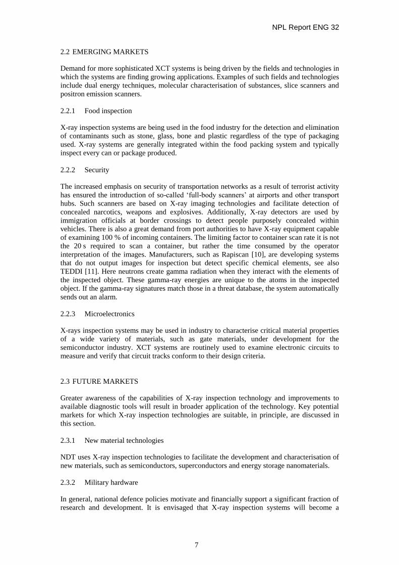
Although technologies such as computed radiography (CR) and XCT are now becoming more
mainstream in industrial application, their rate of adoption in emerging technologies is
comparatively slow. Advances in the healthcare industry (see figure 7) may be used to predict
the rate of adoption of such new technologies for industrial applications.
Performance specifications for X-ray inspection systems are highest for metrology, with a less
stringent requirement for industrial applications and less again for medical applications.
Figure 7. Imaging trends: diagnostic imaging procedure volume by modality [8]
2.3.5 Aerospace demands
Aerospace applications account for about 25 % of the X-ray inspection market. These
applications can be grouped into two categories: flaw detection and dimensional metrology.
Flaws to be detected include cracks, inclusions and voids. Dimensional metrology is used to
compare fabricated components with their original design requirements, to determine:
whether variation in the manufacturing process introduces significant changes to the
final products;
to what extent the final part represents the part envisaged by the designer;
whether the limit of wear on parts conforms to what is deemed acceptable; and
the optimum service period for a given designed component, with greater accuracy.

NPL Report ENG 32
9
2.3.6 Electronics demands
Use of X-ray systems in the electronics industry is growing and such systems have now
become the most widely used tool for the quality control of products such as printed circuit
boards (PCBs), integrated circuits (ICs) and high-density ball grid array (BGA) chips. For this
industry, the main use of X-ray inspection is the detection of flaws such as solder fracture,
voiding and bridging, with metrology currently a lower priority.

NPL Report ENG 32
10
3 XCT HARDWARE
The correct design of the hardware of an XCT system is critical to its ultimate performance.
Further, an understanding of the constituent parts is essential for an appropriate uncertainty
analysis. The following areas of hardware specific to XCT will be the focus of this section.
X-ray source.
Detector.
Computer.
Shielding.
Cooling system.
Sub-systems, such as the manipulation system, vibration isolation, power supply and
environmental control are of wide-spread and long-standing concern to precision dimensional
metrology and have been addressed in detail elsewhere [13-16]. Consequently, they will not
be discussed in detail in this report.
3.1 X-RAY SOURCE
The discovery of X-rays is usually credited to the German physicist Wilhelm Röntgen as he
was the first to systematically study them. He is also responsible for naming them, as in
German, they are referred to as Röntgen Strahlen.
It is believed that the first discovery of X-rays was during the use of Crookes tubes in 1895
when it was realised that the photographic plates were being blackened; for a general
introduction, see [17]. Use of the Crookes tube, invented twenty years previously and related
to modern cathode ray tube display technology, also led to the formal identification of
electrons [18].
X-rays are produced by accelerating electrons through a high voltage, in a vacuum tube, and
allowing the electrons to collide with a metal target. X-rays are produced through two distinct
processes: bremsstrahlung and characteristic radiation.
Bremsstrahlung, or ‘braking radiation’, is caused when an electron approaches very close to
the nucleus of an atom, but does not actually collide with any part of it. During this process,
the electron is affected by the strong nuclear attraction, where the positive charged nucleus
attracts the negatively charged electron. The resulting loss in energy, due to the interaction,
leads to the emission as a photon with the same energy. This sudden deceleration of the
electron gives rise to the radiation known as bremsstrahlung. The probability of this type of
radiation increases with the target’s atomic number (Z) and with increasing energy of the
electrons. The spectrum of bremsstrahlung X-rays is continuous.
NPL Report ENG 32
11
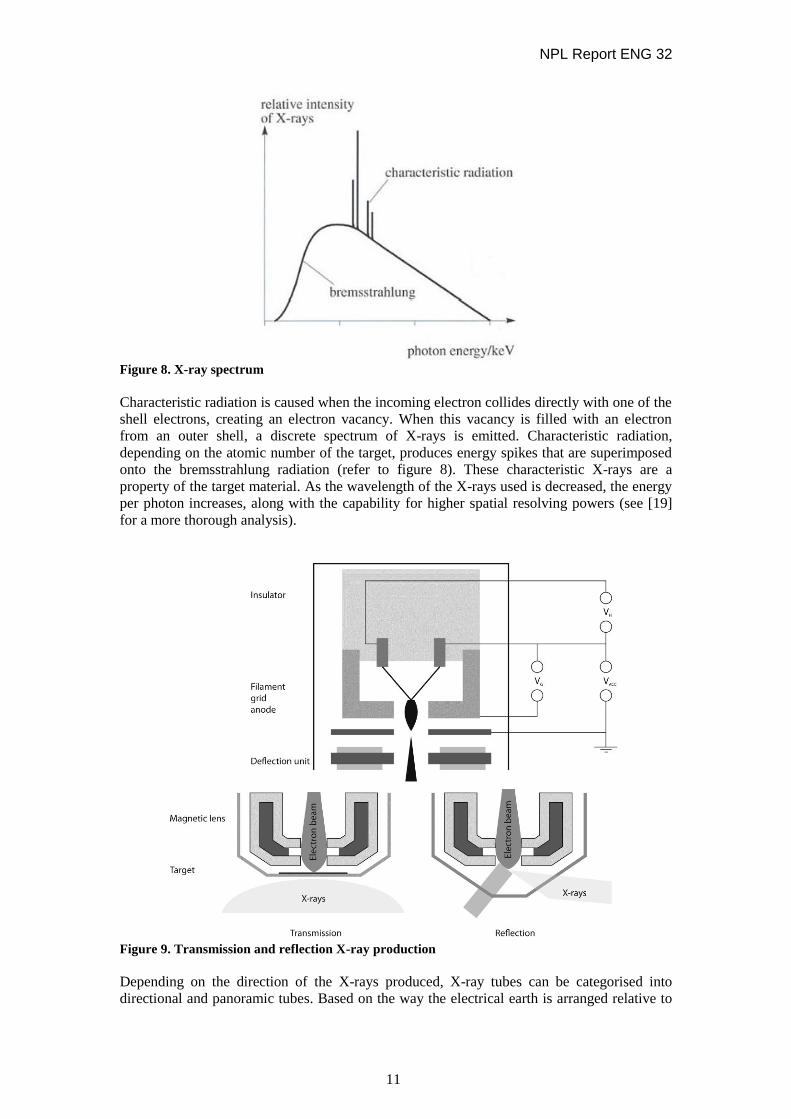
Figure 8. X-ray spectrum
Characteristic radiation is caused when the incoming electron collides directly with one of the
shell electrons, creating an electron vacancy. When this vacancy is filled with an electron
from an outer shell, a discrete spectrum of X-rays is emitted. Characteristic radiation,
depending on the atomic number of the target, produces energy spikes that are superimposed
onto the bremsstrahlung radiation (refer to figure 8). These characteristic X-rays are a
property of the target material. As the wavelength of the X-rays used is decreased, the energy
per photon increases, along with the capability for higher spatial resolving powers (see [19]
for a more thorough analysis).
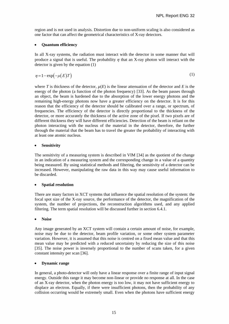
Figure 9. Transmission and reflection X-ray production
Depending on the direction of the X-rays produced, X-ray tubes can be categorised into
directional and panoramic tubes. Based on the way the electrical earth is arranged relative to

NPL Report ENG 32
12
the anode and the cathode, X-ray tubes can be divided into unipolar and bipolar X-ray tubes
[20]. The bipolar tube design can operate at voltages up to 450 kV, whereas the unipolar tube
design can only operate up to 300 kV.
The structure of an X-ray tube is shown in figure 9, where the main parts are a filament
(cathode) and a target (anode). To avoid interaction with molecules of the gas that can
produce lower energy secondary electrons, the X-ray radiation requires a vacuum
environment. The conventional design utilises a sealed evacuated glass tube, whereas metal
and ceramic tubes are increasingly used nowadays due to longer tube life expectancy and
higher heat capacity. It is also common to use open tube designs, where the tube is only
evacuated when powered up [21]. The benefit of using an open tube design is that failed parts,
for example, a burnt target, can be easily changed and the tube can be cleaned and maintained
from time to time. The open tube design is often used in high resolution XCT systems.
The cathode consists of a thin filament (usually tungsten) and the anode contains a small
amount of a tungsten, molybdenum or copper target, which has a high melting point. The
anode is also embedded in to a relatively large amount of copper [22], where the copper helps
to disperse the heat generated. When the X-ray tube is powered up, electrons are produced by
thermionic emission from the electrical heating of a filament. These free electrons are
accelerated towards the anode due to the electric potential. When the electrons hit the anode,
they collide with the atoms of a target object producing X-rays. If the target material is thin
enough, and the electron energy high enough, then X-ray photons are transmitted through the
target. The process is the so called transmission type of X-ray production. However, if the
target is sufficiently thick and the electron energy is sufficiently low, then the X-rays are
emitted in a manner imitating reflection, which is the reflection type of X-ray production.
When the X-ray tube is working, approximately 1 % of the energy generated is emitted as X-
rays and the remaining energy is released as heat. The significant amount of heat generated
can produce damage and can affect the stability of the X-rays generated. Modern designs use
rotating anode tubes so that heat can be dispersed on different parts of the target plate. Apart
from using rotating anode and copper for heat dispersion, recirculating systems of water, oil
or other thermal conductive materials are often used to cool X-ray tubes.
The output X-rays usually pass through a circular aperture or diaphragm (for cone beam) or
through collimating plates (for fan beam) [23].
The focal spot size is important in determining the image quality. Conventional XCT systems
have a focal spot of larger than 1 mm. Microfocus systems have a spot size of between 1 µm
to 1000 µm [23] and nanofocus systems have a spot size of less than 1 µm [24, 25]. Generally
speaking, focal spot size is smaller when lower power is applied. However, with lower power,
the ability for imaging is limited.
The voltage and the current supplied to an X-ray tube are important parameters for controlling
the X-rays that are produced. The voltage (usually in kilovolts), determines the X-ray
spectrum [20]. Increasing the voltage effectively decreases the wavelength of the X-rays
emitted [26] and increasing the current at constant voltage increases the X-ray intensity
without changing the X-ray spectrum.
3.2 X-RAY DETECTORS
As discussed above, the first evidence for X-rays was found unexpectedly by exposing
photographic plates. However, Röntgen also noticed that a barium cyanide coated screen,
stored in the vicinity of the experiment, glowed when the apparatus was energised and ceased
to glow when the apparatus was switched off - this was probably the first encounter with X-

NPL Report ENG 32
13
ray scintillation. There have been several papers investigating the accuracy and reliability of
X-ray detectors, for example [27]. Figure 10 outlines the advances in detectors over the last
forty years [28], where the sensitivity and dynamic range increase significantly.
Figure 10. Advances in detector technology [28]
There are many different types of X-ray detectors. ISO 15708 part 1 [29] splits X-ray
detectors into two groups: ionization detectors and scintillation detectors. More information
about different types of detectors is given in [30], for example, semiconductor detectors and
CCD detectors.
Direct semiconductor detectors
As photographic detectors have evolved, their use in the detection of radiation, both in the
optical and X-ray frequency range, has become commonplace. Semiconductor detectors,
using silicon or germanium doped with lithium, have been around since the 1970s. These
devices produce an electrical current when exposed to X-rays and are generally referred to as
solid state detectors or direct detectors (see figure 11). Some modern direct detectors use
photoconductors, such as amorphous selenium or cadmium telluride coatings on a multi-pixel
microelectronic plate, and the output current is collected by an array of thin film transistors
(TFTs). Currently available systems on the market, such as the FT50m detector [31],
manufactured by Teledyne Dalsa, have claimed pixel size of 5.6 µm × 5.6 µm.
Figure 11. Direct detection of X-ray photons
Direct detection is beneficial due to the increased sensitivity. The detector acts as a single
photon counter. When flux levels are low and a single photon is acting on a single pixel,
direct detection makes it possible to resolve the energies of the incident photons using the
number of counts generated from the detector. This method is known as energy dispersive X-
ray spectroscopy. However, when the photon energy is high (greater than 20 keV), the photon

NPL Report ENG 32
14
passes straight through the detector without any interaction between the detector and the
photon. Overexposure to X-rays may also damage the CCD. This can manifest itself as an
increase in dark current [32] and a voltage shift of the sensor. Sensors are generally small in
area, for example 25 mm × 25 mm; cost increases dramatically with size. To reduce shot
noise, detectors are sometimes cooled using liquid nitrogen, Peltier cooling or other methods.
Scintillation detectors
In general, scintillation is a flash of visible light produced in a transparent material by an
ionisation event. Scintillation detectors can convert high-energy X-ray photons into lower
energy photons in the visible wavelength range, and these optical photons can then be
detected by means of a photomultiplier tube or a photodiode. Scintillation detectors use this
principle, and have the advantage that they are more sensitive to lower doses of X-rays.
A scintillator and a flat panel detector (FPD) together form an indirect FPD. The scintillator
coating converts the X-rays to visible light and the photo diode or photomultiplier tube then
converts the visible light to a digital output. Hence, this type of detector is also termed an
‘indirect’ detector. Typical materials used for indirect FPDs would be sodium-activated
caesium iodide on a substrate of an amorphous silicon detector (see figure 12).
Figure 12. Structure of a scintillation detector [28]
3.3 PROPERTIES OF XCT DETECTORS
The most important detector characteristics are: field coverage, geometrical characteristics,
quantum efficiency, sensitivity, spatial resolution, noise characteristics, dynamic range,
uniformity, acquisition speed, frame rate and cost [33].
Field coverage
If parts of the object under examination are not detected at every position, there will be an
error in the final computation that cannot be determined. This lack of information causes
errors in XCT scanning – see section 5.4 for more details.
Geometrical characteristics
Due to the presence of sensor circuitry adjacent to each pixel, a small but significant, fraction
of the display area is insensitive to incoming radiation. This area is referred to as the ‘dead’
NPL Report ENG 32
15
region and is not used in analysis. Distortion due to non-uniform scaling is also considered as
one factor that can affect the geometrical characteristics of X-ray detectors.
Quantum efficiency
In all X-ray systems, the radiation must interact with the detector in some manner that will
produce a signal that is useful. The probability η that an X-ray photon will interact with the
detector is given by the equation (1)
1 exp η μ E T (1)
where T is thickness of the detector, µ(E) is the linear attenuation of the detector and E is the
energy of the photon (a function of the photon frequency) [33]. As the beam passes through
an object, the beam is hardened due to the absorption of the lower energy photons and the
remaining high-energy photons now have a greater efficiency on the detector. It is for this
reason that the efficiency of the detector should be calibrated over a range, or spectrum, of
frequencies. The efficiency of the detector is directly proportional to the thickness of the
detector, or more accurately the thickness of the active zone of the pixel. If two pixels are of
different thickness they will have different efficiencies. Detection of the beam is reliant on the
photon interacting with the nucleus of the material in the detector, therefore, the further
through the material that the beam has to travel the greater the probability of interacting with
at least one atomic nucleus.
Sensitivity
The sensitivity of a measuring system is described in VIM [34] as the quotient of the change
in an indication of a measuring system and the corresponding change in a value of a quantity
being measured. By using statistical methods and filtering, the sensitivity of a detector can be
increased. However, manipulating the raw data in this way may cause useful information to
be discarded.
Spatial resolution
There are many factors in XCT systems that influence the spatial resolution of the system: the
focal spot size of the X-ray source, the performance of the detector, the magnification of the
system, the number of projections, the reconstruction algorithms used, and any applied
filtering. The term spatial resolution will be discussed further in section 6.4.1.
Noise
Any image generated by an XCT system will contain a certain amount of noise, for example,
noise may be due to the detector, beam profile variation, or some other system parameter
variation. However, it is assumed that this noise is centred on a fixed mean value and that this
mean value may be predicted with a reduced uncertainty by reducing the size of this noise
[35]. The noise power is inversely proportional to the number of scans taken, for a given
constant intensity per scan [36].
Dynamic range
In general, a photo-detector will only have a linear response over a finite range of input signal
energy. Outside this range it may become non-linear or provide no response at all. In the case
of an X-ray detector, when the photon energy is too low, it may not have sufficient energy to
displace an electron. Equally, if there were insufficient photons, then the probability of any
collision occurring would be extremely small. Even when the photons have sufficient energy
NPL Report ENG 32
16
and number to generate a signal, this signal may be lost in the noise. The lower level of this
input that cannot be discriminated from the detector noise is termed the noise equivalent
input.
At the other end of the scale, for the case where the energy of the photon is high and the
number of photons large, the detector may be unable to discriminate between two adjacent
photons, resulting in a saturation effect known as blooming. In some cases the dynamic range
of a detector is related to the signal-to-noise ratio, which is equal to the ratio of the average
signal intensity over the standard deviation of the noise.
Uniformity
Uniformity describes the variation of response to a constant, spatially uniform incident X-ray
illumination across the face of the total receptor area. Areas where the detector does not have
the same sensitivity can be corrected for in software, generally by using a look-up table
derived from a characterisation of the detector.
Capture duration
There are many individual parts that contribute to the capture and processing of the data for
XCT systems. Measuring volume, resolution and speed of processing are some examples.
Currently, objects as large as automobile cylinder heads can be scanned, using medical XCT
systems in a few minutes with a resolution on the order of 100 µm. On an industrial XCT
system, the scan can take ten to twenty hours with a resolution of a few micrometres.
Weight limit
As a general rule, if the measuring volume of an XCT increases, so too does the weight
carrying capability. However, XCT systems rely on the relative absorption of the photons - if
all the X-ray photons are absorbed before reaching the detector then there are no data for
analysis. Materials with high atomic number are more efficient absorbers of X-ray photons.
The largest volume that can be measured is that volume that allows sufficient X-ray photons
to reach the detector, to allow a confident analysis. As different materials have different
densities, this means that the maximum volume of the object is dependent on the object’s
density.
3.4 PC HARDWARE
After the images have been acquired from the detector for each of the rotational positions, the
set of images are passed through a series of computations that translate this information into
voxels. The process can be time-consuming and requires a lot of computing power. Hence,
the capability of the computer is critical. Generally, three components have to be considered
when building a computer for XCT data reconstruction and data analyses. These components
are central processing unit (CPU), random-access memory (RAM) and graphic cards. Recent
development in multi-core processors and advanced graphic cards with graphics processing
units (GPUs) can significantly accelerate the speed when handling large amounts of data and
increase speed of image decoding. The flexibility for the user to choose a suitable size of
computer memory allows large amounts of data to be read. At the time of writing, it is
common to use a computer with 96 gigabyte of RAM in the computers for XCT systems. It is
believed that this figure will be dramatically increased shortly. It is also noticed that super-
computing power is expensive. However, the development of grid computing offers other
chances to significantly improve the efficiency of data analyses, where the cost can be shared
between a few users.

NPL Report ENG 32
17
3.5 SHIELDING
Health and safety is important when operating an XCT system. Critical parameters, such as
beam power, workload, scatter and leakage, must be taken into account when calculating the
required shielding [37]. The traditional material used in the shielding of harmful X-rays is
lead, due to its high density (11340 kg m-3
) and atomic number (82). As the energy of the X-
ray beam increases then the resultant thickness of the shielding needs to be increased.
3.6 COOLING SYSTEM
Because of the low efficiency of the X-ray production process, XCT systems, especially
systems generating high power, require cooling systems due to the amount of heat dissipated
by the target. By keeping the system at a fixed temperature, the instability of the system
through thermal effects may be greatly reduced. By cooling the detector, the signal-to-noise
ratio may also be increased. As discussed in section 3.1, the cooling of an X-ray tube is
critical in XCT systems. However, an external cooling system is also important to maintain
temperature stability in the measurement chamber. More detailed information regarding
cooling can be found elsewhere [38-41].
NPL Report ENG 32
18
4 DATA PROCESSING
Data processing plays an important role in XCT technology. Without the reconstruction
process, the XCT images are simply radiographs as provided by conventional radiology. This
section reviews the data reconstruction process and the software available on the market.
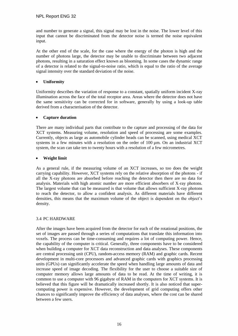
Assuming an XCT system with a detector of M N pixels and P projections with different
rotation angles has been taken for one measurement, the reconstruction process involves
solving an M N P cubic matrix of attenuation coefficients (see figure 13).
Figure 13. XCT cubic matrix of attenuation coefficients
For XCT systems, the X-ray beam penetrates the sample and projects on to the detector. The
resultant radiography image is the projection of the sample and the intensity of each pixel is a
function of the attenuation coefficient and the distance the X-ray travels within the sample.
The projection can be calculated using a Radon transforms, see equation (2) [42], where the
Radon transform of a ray passing through a medium f(x) with length L is the line integral and
projection is given by
xx dfLpfL (2)
The task of XCT reconstruction is to find )(xf given a knowledge of )(Lpf . This process is
called backprojection, which can be solved using an inverse Radon transform.
The Radon transform and its inverse function form the mathematical basis for reconstructing
tomographic images from the projection data. The images in figure 14 and figure 15 illustrate
the Radon transform and inverse Radon transform of the image of a square object. However,
the backprojection based on an inverse Radon transform process results in a blurred image.
This can be minimised by applying a filtering process before backprojection (see figure 15).
The filtering used in the reconstruction is generally a low pass filter type. There are many
filters that can be used for reconstruction purposes. Examples include the Shepp-Logan, Laks,
Ramachandran and Ramp filters [43-45]. Some typical filters are presented in figure 16.

NPL Report ENG 32
19
Figure 14. Illustration of Radon transform for a square object (top) image of a square (bottom)
Radon transform of the square image from 0 to 180
Figure 15. Inverse of Radon transform (left) original square image (middle) image reconstructed
using filtered backprojection process (right) image calculated using unfiltered backprojection
process
20 40 60 80 100
10
20
30
40
50
60
70
80
90
100 0
0.2
0.4
0.6
0.8
1
(degrees)
Pro
jection d
ispla
cem
ent
0 50 100 150
-60
-40
-20
0
20
40
6010
20
30
40
50
60
70
Original Filtered backprojection Unfiltered backprojection

NPL Report ENG 32
20
Figure 16. Operation of typical filters [46]
Given the potential benefits, it is common to filter the projection data before applying the
backprojection process. However, variants exist where the backprojection is performed before
the filtering procedure. Filtered backprojection algorithms are more accurate than the image
reconstructed by backprojection filtering algorithms. The differences resulting from this
change in processing order is discussed elsewhere [47].
4.1 RECONSTRUCTION OF CONE-BEAM XCT
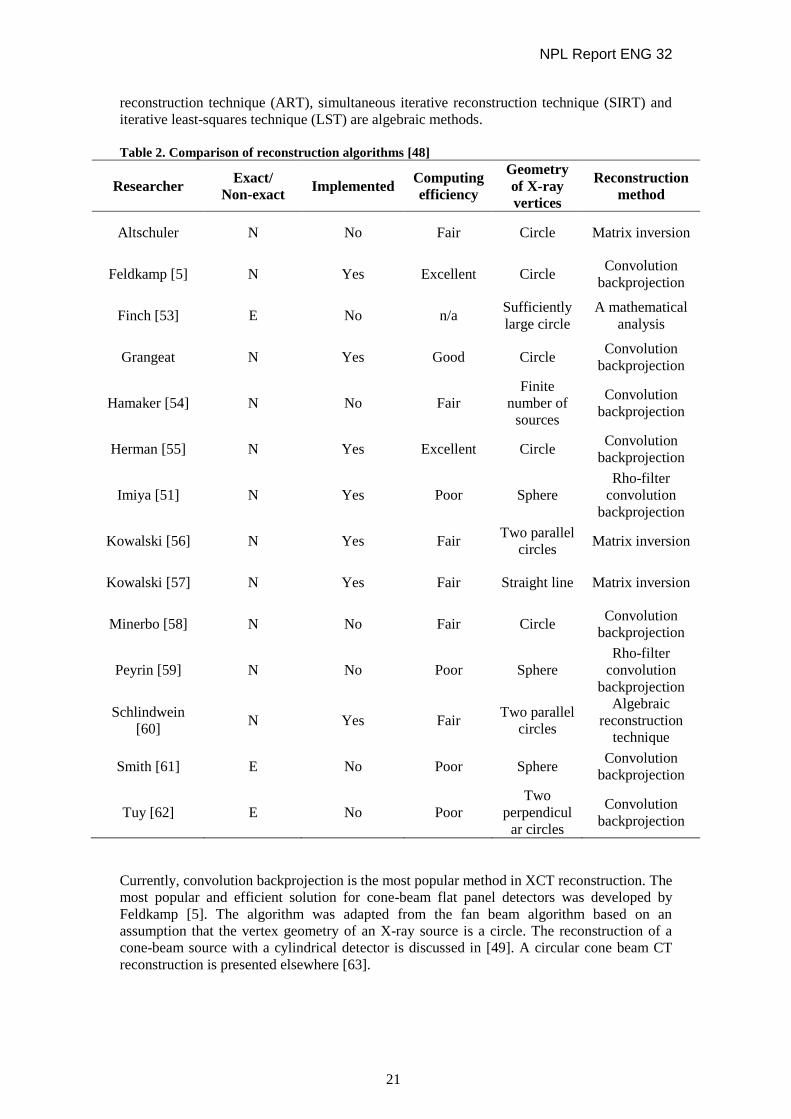
Many researchers have considered the reconstruction of cone-beam data. Key algorithms are
compared in [48] (and see table 2). The following discussion is based on the algorithms listed
in table 2.
There are a number of aspects that should be considered when evaluating different
reconstruction algorithms. The first aspect is whether the algorithm is exact or non-exact. An
exact algorithm is mathematically correct if the data are noise-free and captured with
sufficient density along the source trajectory with a detector array having sufficient detector
element density. Non-exact algorithms are more flexible in the case where there are missing
data points or there are insufficient projection data in a given angular interval [49]. The
geometry (trajectory or path) of the X-ray vertex point is also important. The term vertex
point refers to the position of the X-ray source [50]. Smith [48] concluded that one scan has
complete information about an object if, on every plane that intersects the object, there lies a
vertex. For example, vertex geometries of two periods of a sinusoid on a cylinder provide
complete information about an object. However, the implementation of scan with complex
vertex geometry can be poor. For example, the method developed in reference [51], which
requires a sphere vertex geometry, is difficult to achieve in practice. Apart from those aspects
considered above, the implementation and efficiency of those algorithms have been
considered in table 2.
The two main categories of algorithms are ‘analytic’ and ‘algebraic’, where algebraic
algorithms demand more computing power than analytic algorithms. Thus, due to high
reconstruction speed, the analytic algorithms are more efficient in practice [52]. Convolution
backprojection, matrix inversion and Fourier transform are analytic algorithms. The algebraic
NPL Report ENG 32
21
reconstruction technique (ART), simultaneous iterative reconstruction technique (SIRT) and
iterative least-squares technique (LST) are algebraic methods.
Table 2. Comparison of reconstruction algorithms [48]
Researcher Exact/
Non-exact Implemented
Computing
efficiency
Geometry
of X-ray
vertices
Reconstruction
method
Altschuler N No Fair Circle Matrix inversion
Feldkamp [5] N Yes Excellent Circle Convolution
backprojection
Finch [53] E No n/a Sufficiently
large circle
A mathematical
analysis
Grangeat N Yes Good Circle Convolution
backprojection
Hamaker [54] N No Fair
Finite
number of
sources
Convolution
backprojection
Herman [55] N Yes Excellent Circle Convolution
backprojection
Imiya [51] N Yes Poor Sphere
Rho-filter
convolution
backprojection
Kowalski [56] N Yes Fair Two parallel
circles Matrix inversion
Kowalski [57] N Yes Fair Straight line Matrix inversion
Minerbo [58] N No Fair Circle Convolution
backprojection
Peyrin [59] N No Poor Sphere
Rho-filter
convolution
backprojection
Schlindwein
[60] N Yes Fair
Two parallel
circles
Algebraic
reconstruction
technique
Smith [61] E No Poor Sphere Convolution
backprojection
Tuy [62] E No Poor
Two
perpendicul
ar circles
Convolution
backprojection
Currently, convolution backprojection is the most popular method in XCT reconstruction. The
most popular and efficient solution for cone-beam flat panel detectors was developed by
Feldkamp [5]. The algorithm was adapted from the fan beam algorithm based on an
assumption that the vertex geometry of an X-ray source is a circle. The reconstruction of a
cone-beam source with a cylindrical detector is discussed in [49]. A circular cone beam CT
reconstruction is presented elsewhere [63].

NPL Report ENG 32
22
Most XCT manufacturers develop proprietary reconstruction software. For example, Nikon
provides CT pro [64] and GE provides phoenix datos|x [65] to reconstruct data. The most
common reconstruction algorithm used in practice is the filtered backprojection algorithm.
4.2 COMMERCIAL VISUALISATION SOFTWARE PACKAGES
There are a number of commercial software packages available for volumetric visualisation of
reconstructed XCT data. Most of these packages provide basic functions such as visualisation
and segmentation. Some brief information on these software packages is provided in this
section.
VGStudio MAX was developed by Volume Graphics for the visualization and analysis of
XCT data. The company was founded in 1997 in Heidelberg, Germany. Four add-on modules
are available for end-users. These modules are “Coordinate Measurement”, “Nominal/Actual
Comparison”, “Porosity/Inclusion Analysis” and “Wall Thickness Analysis”.
Website: www.volumegraphics.com/ Accessed on 1st August 2011
Avizo is a commercial software package that is available to visualise volumetric data. Its
predecessor was Amira and it was originally developed by Visualization and Data Analysis
Group. Avizo has been commercially developed and distributed by Visualization Sciences
Group. The software also has four extension modules designed for different purposes. These
are Avizo Earth for geosciences and the oil and gas industries, Avizo Wind for simulation
data, Avizo Fire for materials science and Avizo Green for environmental data.
Website: www.vsg3d.com/ Accessed on 1st August 2011
Simpleware is a volumetric data processing software package with a focus on converting
volumetric data into CAD and finite element models. Simpleware was developed by
Simpleware Ltd., a privately owned company based in Exeter, UK. The core software is
ScanIP, in which the user can segment and export the data. Simpleware has two extended
modules, ScanCAD for mesh generation and ScanFE for CAD integration.
Website: www.simpleware.com/ Accessed on 1st August 2011
4.3 FREEWARE
Apart from commercial software, there are also many freeware packages available over the
Internet. Many of the freeware packages are capable of running on multiple software
platforms and the source code is freely available to end-users.
Drishiti was developed by Ajay Limaye at the Australian National University. The software
offers many useful visualisation features for volumetric data.
Website: anusf.anu.edu.au/Vizlab/drishti/index.shtml Accessed on 1st August 2011
VolPack was developed by Philippe Lacroute at the Stanford Computer Graphics Laboratory.
The software was based on a family of fast volume rendering algorithms [66]. The library is
intended for use in C or C++ programs.
Website: graphics.stanford.edu/software/volpack/ Accessed on 1st August 2011
ImageJ was developed by Wayne Rasband at the National Institutes of Health in United
States. It was written in Java and the source code is free and in the public domain. The
software offers users simple solutions to calculate area and pixel values of user-defined
selections. It can also calculate distances and angles and provides plugins such as filters and
segmentation for advanced users.
Website: rsbweb.nih.gov/ij/index.html Accessed on 1st August 2011

NPL Report ENG 32
23
Visualization Toolkit (VTK) is an open-source software system for volumetric computer
graphics, imaging processing and visualization. It utilises a C++ class library and interpreted
interface layers including Java and Python. VTK supports many features such as polygon
reduction, mesh smoothing and parallel processing.
Website: www.vtk.org/ Accessed on 1st August 2011
Paraview is an open-source, multi-platform software for visualization and data analyses,
developed by Sandia National Laboratories, in conjunction with NVIDIA Corporation and
Kitware Inc. As it uses distributed memory computing resources, the software is capable of
parallel rendering and can be used to process very large datasets.
Website: www.paraview.org/ Accessed on 1st August 2011
NPL Report ENG 32
24
5 SYSTEMATIC ERRORS IN XCT
There are many sources of systematic error related to XCT technologies. These errors have
been reviewed previously [23, 67]. The most common systematic errors are reviewed in this
section, for example, the errors related to the X-ray tube, the detector and the physical
characteristic of XCT systems. Errors related to the setup of the sample are also briefly
discussed.
The definition of the term ‘artefact’ used in the following is given in ISO 15708 part 1 [29]
as: the discrepancy between the actual value of some physical property of an object and the
map of that property generated by a XCT imaging process.
5.1 BEAM DRIFT
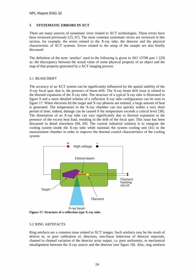
The accuracy of an XCT system can be significantly influenced by the spatial stability of the
X-ray focal spot, that is, the presence of beam drift. The X-ray beam drift issue is related to
the thermal expansion of the X-ray tube. The structure of a typical X-ray tube is illustrated in
figure 9 and a more detailed schema of a reflection X-ray tube configuration can be seen in
figure 17. When electrons hit the target and X-ray photons are emitted, a large amount of heat
is generated. The temperature in the X-ray chamber can rise quickly within a very short
period of time; indeed, damage can be caused if the temperature exceeds a critical level [38].
The dimensions of an X-ray tube can vary significantly due to thermal expansion in the
presence of the excess heat load, resulting in the drift of the focal spot. This issue has been
discussed in detail elsewhere [68, 69]. The current industrial solution is to integrate the
cooling system inside the X-ray tube while maintain the system cooling unit [41] in the
measurement chamber in order to improve the thermal control characteristics of the cooling
system.
Figure 17. Structure of a reflection type X-ray tube
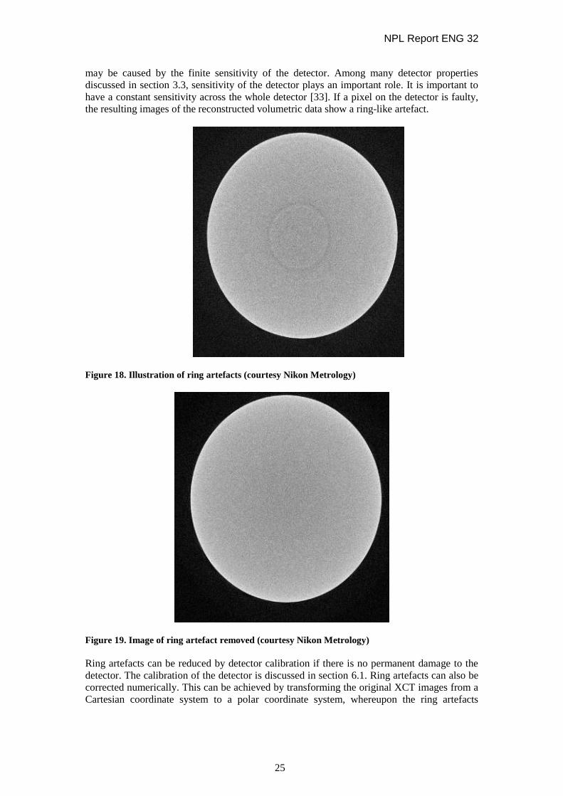
5.2 RING ARTEFACTS
Ring artefacts are a common issue related to XCT images. Such artefacts may be the result of
defects in, or poor calibration of, detectors, non-linear behaviour of detector materials,
channel to channel variation of the detector array output, i.e. poor uniformity, or mechanical
misalignment between the X-ray source and the detector (see figure 18). Also, ring artefacts
NPL Report ENG 32
25
may be caused by the finite sensitivity of the detector. Among many detector properties
discussed in section 3.3, sensitivity of the detector plays an important role. It is important to
have a constant sensitivity across the whole detector [33]. If a pixel on the detector is faulty,
the resulting images of the reconstructed volumetric data show a ring-like artefact.
Figure 18. Illustration of ring artefacts (courtesy Nikon Metrology)
Figure 19. Image of ring artefact removed (courtesy Nikon Metrology)
Ring artefacts can be reduced by detector calibration if there is no permanent damage to the
detector. The calibration of the detector is discussed in section 6.1. Ring artefacts can also be
corrected numerically. This can be achieved by transforming the original XCT images from a
Cartesian coordinate system to a polar coordinate system, whereupon the ring artefacts
NPL Report ENG 32
26
become a line and can be removed [70]. Figure 18 shows an image with ring artefacts and
figure 19 shows the image with the ring artefacts removed.
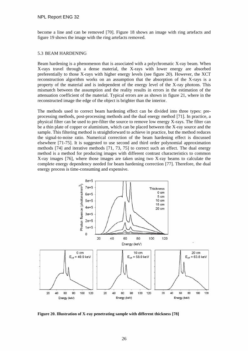
5.3 BEAM HARDENING
Beam hardening is a phenomenon that is associated with a polychromatic X-ray beam. When
X-rays travel through a dense material, the X-rays with lower energy are absorbed
preferentially to those X-rays with higher energy levels (see figure 20). However, the XCT
reconstruction algorithm works on an assumption that the absorption of the X-rays is a
property of the material and is independent of the energy level of the X-ray photons. This
mismatch between the assumption and the reality results in errors in the estimation of the
attenuation coefficient of the material. Typical errors are as shown in figure 21, where in the
reconstructed image the edge of the object is brighter than the interior.
The methods used to correct beam hardening effect can be divided into three types: pre-
processing methods, post-processing methods and the dual energy method [71]. In practice, a
physical filter can be used to pre-filter the source to remove low energy X-rays. The filter can
be a thin plate of copper or aluminium, which can be placed between the X-ray source and the
sample. This filtering method is straightforward to achieve in practice, but the method reduces
the signal-to-noise ratio. Numerical correction of the beam hardening effect is discussed
elsewhere [71-75]. It is suggested to use second and third order polynomial approximation
methods [74] and iterative methods [71, 73, 75] to correct such an effect. The dual energy
method is a method for producing images with different contrast characteristics to common
X-ray images [76], where those images are taken using two X-ray beams to calculate the
complete energy dependency needed for beam hardening correction [77]. Therefore, the dual
energy process is time-consuming and expensive.
Figure 20. Illustration of X-ray penetrating sample with different thickness [78]

NPL Report ENG 32
27
Two common artefacts resulting from beam hardening effects are ‘streak’ artefacts and
‘cupping’ artefacts [67].
Figure 21. Beam hardening effects (left) an image without filtering (right) an image with a 1 mm
thick copper filter (courtesy Nikon Metrology)
An example of streak artefacts can be seen in figure 22. Streak (or metal) artefacts are
common in XCT images with typical black and white lines, which cause significant
degradation in the X-ray image. Streak artefacts can be caused by many factors. For example,
a sample with high-density metal parts can attenuate part or all X-ray energies, which leads to
incorrect measurements of the objects behind the metal part. This can be corrected by raising
the energy level of the X-ray source [79]. Streak artefacts can also be caused if the object is
moved during measurement, insufficient rotational sampling points are specified, or if the
instrument coordinate system is misaligned [80]. Streak artefacts can be corrected using a
linearization technique based on a physical model [81].
Figure 22. Illustration of ring artefacts and streak artefacts
NPL Report ENG 32
28
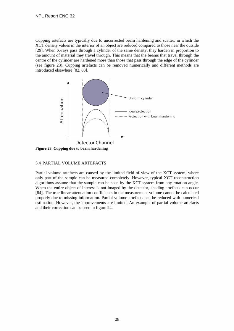
Cupping artefacts are typically due to uncorrected beam hardening and scatter, in which the
XCT density values in the interior of an object are reduced compared to those near the outside
[29]. When X-rays pass through a cylinder of the same density, they harden in proportion to
the amount of material they travel through. This means that the beams that travel through the
centre of the cylinder are hardened more than those that pass through the edge of the cylinder
(see figure 23). Cupping artefacts can be removed numerically and different methods are
introduced elsewhere [82, 83].
Figure 23. Cupping due to beam hardening
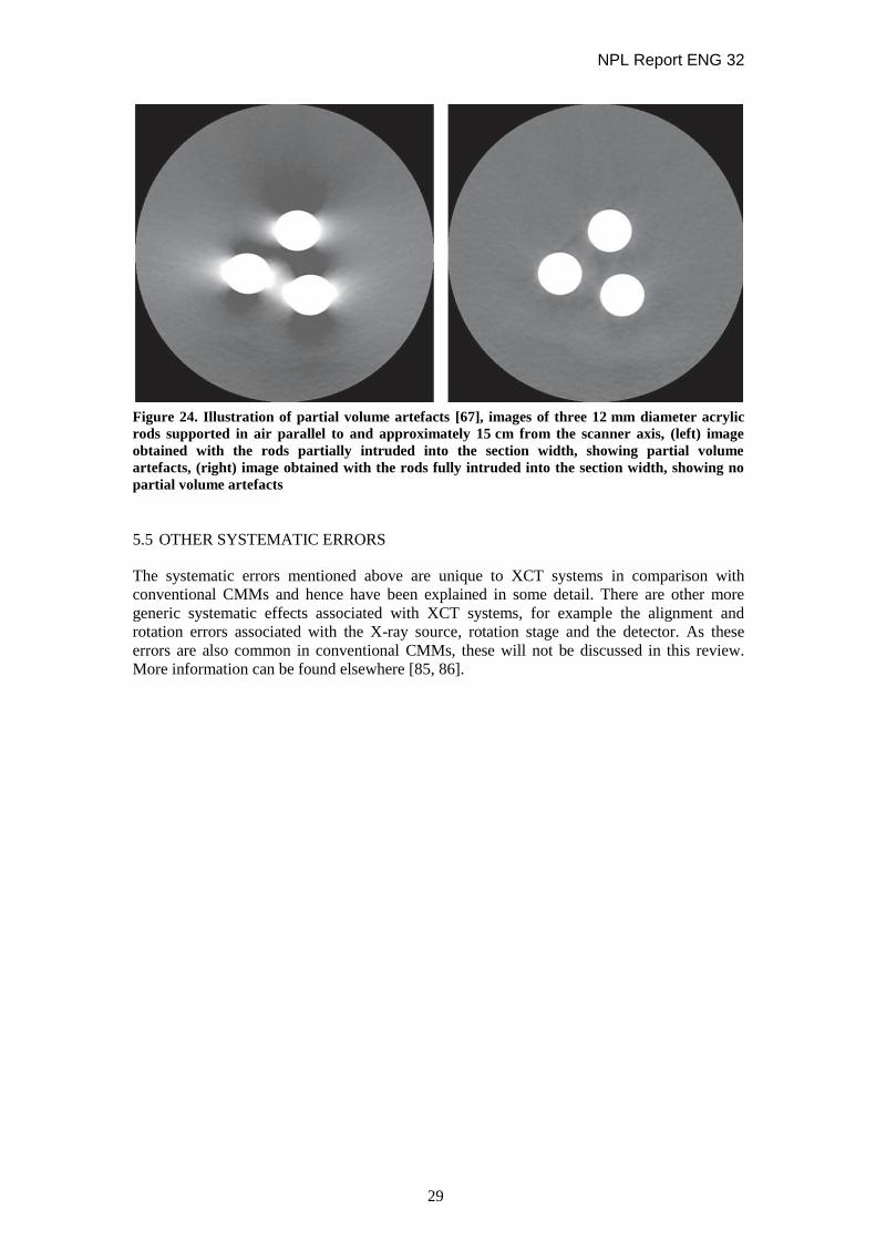
5.4 PARTIAL VOLUME ARTEFACTS
Partial volume artefacts are caused by the limited field of view of the XCT system, where
only part of the sample can be measured completely. However, typical XCT reconstruction
algorithms assume that the sample can be seen by the XCT system from any rotation angle.
When the entire object of interest is not imaged by the detector, shading artefacts can occur
[84]. The true linear attenuation coefficients in the measurement volume cannot be calculated
properly due to missing information. Partial volume artefacts can be reduced with numerical
estimation. However, the improvements are limited. An example of partial volume artefacts
and their correction can be seen in figure 24.
NPL Report ENG 32
29
Figure 24. Illustration of partial volume artefacts [67], images of three 12 mm diameter acrylic
rods supported in air parallel to and approximately 15 cm from the scanner axis, (left) image
obtained with the rods partially intruded into the section width, showing partial volume
artefacts, (right) image obtained with the rods fully intruded into the section width, showing no
partial volume artefacts
5.5 OTHER SYSTEMATIC ERRORS
The systematic errors mentioned above are unique to XCT systems in comparison with
conventional CMMs and hence have been explained in some detail. There are other more
generic systematic effects associated with XCT systems, for example the alignment and
rotation errors associated with the X-ray source, rotation stage and the detector. As these
errors are also common in conventional CMMs, these will not be discussed in this review.
More information can be found elsewhere [85, 86].
NPL Report ENG 32
30
6 XCT SYSTEM CALIBRATION AND VERIFICATION
Calibration and verification are two processes that are used to evaluate a measurement
system. Information on related terminology and definitions can be found in ISO 9000 [87]
and VIM [34].
Calibration
Calibration is the process of comparing the measurement result obtained from the instrument
under investigation against that of a known standard, which has an unbroken chain back to
national or international standards, with each comparison having a stated uncertainty.
Verification
Verification is analogous to calibration but returns only a pass/fail result that indicates
whether the instrument has been found to be operating within a defined specification, such as
published performance data provided by the instrument manufacturer.
6.1 XCT SYSTEM CALIBRATION
When calibrating a system, it is important to know the influence factors that may lead to
systematic errors. Examples of influence factors that are known to contribute to errors in
dimensional data obtained from a XCT system are listed in table 3. This is not an exhaustive
list and, as the subtleties of operation of each XCT system become better understood, more
error sources are likely to be added.
Table 3. Examples of error sources in 3D XCT measurements
Type of cause Influence factors
Environment temperature, humidity, vibration, dust
Object surface roughness, penetration depth, material composition
Detector sensitivity, dynamics, quantum efficiency, internal scattering
X-ray source spectral characteristics, focus properties, opening angle,
stability and thermal drift
Manipulation system geometrical errors, mechanical stability, wobbling
Data processing reconstruction, threshold determination, filtering, algorithm
implementation, artefacts
Other factors clamping system, object orientation, source current, image
statistics
There is increasing interest in XCT calibration in recent years, see for example [14, 15, 88-
99]. Due to the importance of the X-ray source and detectors, their calibration is discussed in
detail in this section.
Current studies of X-ray sources focus on the characteristics of the focal spot, i.e., the size
and shape [92]. Measurement methods for spot size are discussed elsewhere [93-95].
International standard BS EN 12543 part 5 [96] specifies a method for the measurement of
focal spot dimensions between 5 µm and 300 µm and the study has been extended to sub-
micrometre spot sizes in [97]. However, the effect of X-ray tube current and voltage on focal
spot size should be taken into account [100, 101]. Also, the dimensional stability of the focal
spot is important as discussed in sections 3.1 and 5.1.
NPL Report ENG 32
31
XCT systems operate by determining the difference in intensity between the initial emitted
radiation and the absorbed radiation. It is, therefore, critical that these two intensity values are
accurately determined. To this end, the detector system needs to be evaluated [102] with and
without the presence of radiation. There is commercially available equipment for the
calibration of cone beam XCT detectors [103] through the use of calibration standards.
Defining the boundary between one material and the other becomes more difficult if the
atomic numbers of the two interfacing materials are closely matched - this is due to the
variation in what is referred to as the greyscale.
The calibration of a detector is generally carried out by analysing the detector signals with
and without incident X-ray illumination. Each pixel in the detector is examined for each case,
and its output used to give a calibration response for the radiation dose. Pixels that have no
response are assigned the average value of the adjacent pixels in order to compute the
associated voxel densities. Noise in the detector has a tendency to decrease the difference in
the greyscale between the two materials.
6.2 XCT SYSTEM VERIFICATION
CMMs are generally categorised into two types: contact and non-contact systems. Tactile
CMM systems belong to the contact type, and optical systems and XCT systems effectively
belong to the non-contact type.
In 2000, the release of ISO 10360 part 1 [104] provided the latest definition of ‘acceptance
test’ and ‘reverification test’ for CMMs. ISO 10360 part 1 was further extended with the
focus on tactile systems [105-109] and recently added guidance for CMMs with imaging
probing systems [110]. Based on the ISO 10360 standards, the verification of CMM systems
was detailed in [111]. The definition of CMM verification is given as ‘a task carried out at
periodic intervals (often annually) to determine if the CMM still meets the manufacturer’s
specification.’
The principle of tactile system verification is detailed in ISO 10360 part 2 and part 5 [105,
108]. The standard recommends comparing the indicated value of five different calibrated and
traceable test lengths relative to their calibrated values. The acceptance criterion is that the
length error and repeatability, with the consideration of uncertainty, is within the maximum
permissible errors specified by the manufacturer. The procedure of imaging probing system
verification in ISO 10360 part 7 [110] and contains more detail compared to that related to
tactile systems. ISO 10360 part 7 requires the investigation of squareness errors and probing
errors.
Currently, there is no international standard that provides comprehensive guidance for system
verification for XCT. Although an XCT system is effectively a CMM, its operation is not
straightforward compared to conventional tactile and optical systems and the errors associated
with the measurements are of a different nature as discussed in section 5.
6.3 INTERNATIONAL STANDARDS FOR XCT TECHNOLOGY
Although there is no published international standard that covers the calibration and
verification of XCT systems as discussed in section 6.1 and 6.2, more awareness is being
given to the field by a number of international standard committees. There are currently a
number of standards related to XCT technology in published or draft form (see table 4).
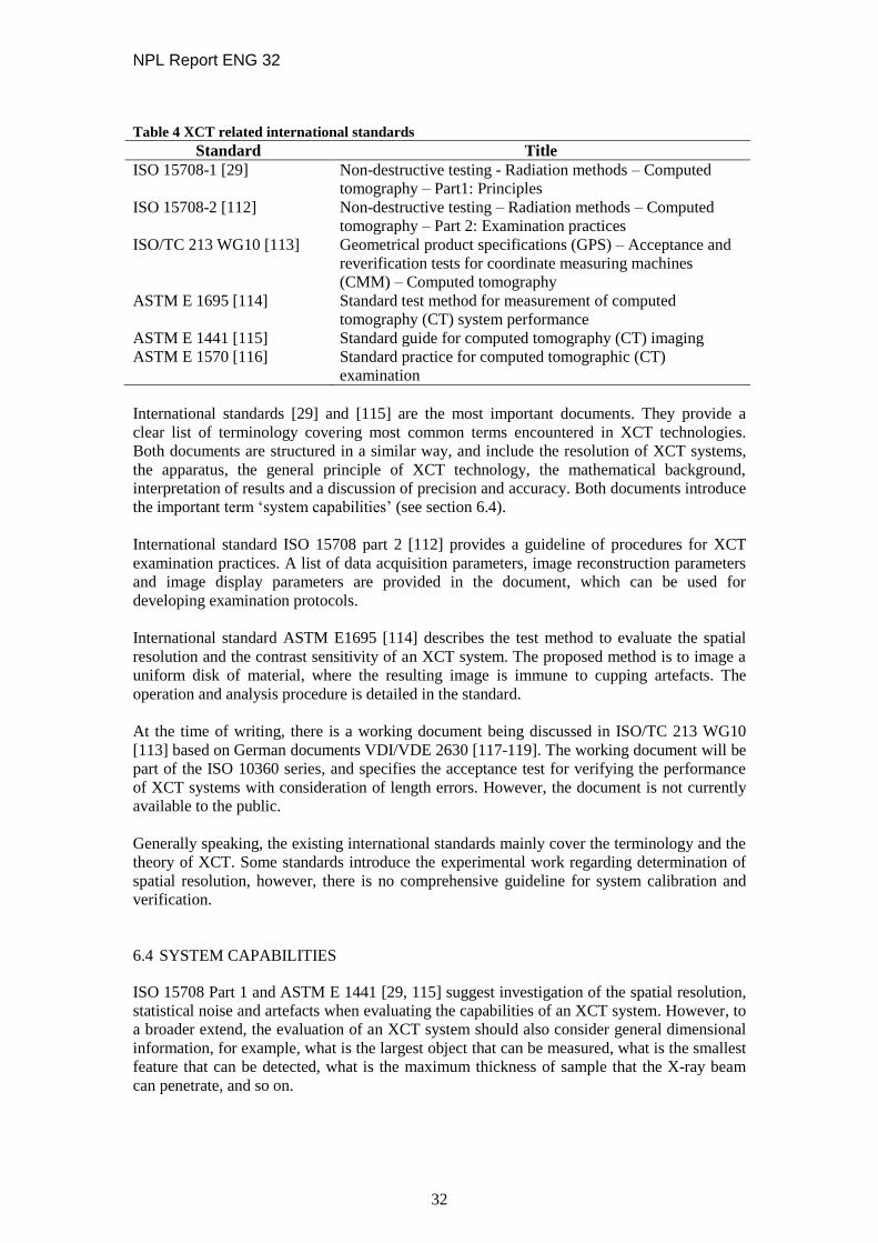
NPL Report ENG 32
32
Table 4 XCT related international standards
Standard Title
ISO 15708-1 [29] Non-destructive testing - Radiation methods – Computed
tomography – Part1: Principles
ISO 15708-2 [112] Non-destructive testing – Radiation methods – Computed
tomography – Part 2: Examination practices
ISO/TC 213 WG10 [113] Geometrical product specifications (GPS) – Acceptance and
reverification tests for coordinate measuring machines
(CMM) – Computed tomography
ASTM E 1695 [114] Standard test method for measurement of computed
tomography (CT) system performance
ASTM E 1441 [115] Standard guide for computed tomography (CT) imaging
ASTM E 1570 [116] Standard practice for computed tomographic (CT)
examination
International standards [29] and [115] are the most important documents. They provide a
clear list of terminology covering most common terms encountered in XCT technologies.
Both documents are structured in a similar way, and include the resolution of XCT systems,
the apparatus, the general principle of XCT technology, the mathematical background,
interpretation of results and a discussion of precision and accuracy. Both documents introduce
the important term ‘system capabilities’ (see section 6.4).
International standard ISO 15708 part 2 [112] provides a guideline of procedures for XCT
examination practices. A list of data acquisition parameters, image reconstruction parameters
and image display parameters are provided in the document, which can be used for
developing examination protocols.
International standard ASTM E1695 [114] describes the test method to evaluate the spatial
resolution and the contrast sensitivity of an XCT system. The proposed method is to image a
uniform disk of material, where the resulting image is immune to cupping artefacts. The
operation and analysis procedure is detailed in the standard.
At the time of writing, there is a working document being discussed in ISO/TC 213 WG10
[113] based on German documents VDI/VDE 2630 [117-119]. The working document will be
part of the ISO 10360 series, and specifies the acceptance test for verifying the performance
of XCT systems with consideration of length errors. However, the document is not currently
available to the public.
Generally speaking, the existing international standards mainly cover the terminology and the
theory of XCT. Some standards introduce the experimental work regarding determination of
spatial resolution, however, there is no comprehensive guideline for system calibration and
verification.
6.4 SYSTEM CAPABILITIES
ISO 15708 Part 1 and ASTM E 1441 [29, 115] suggest investigation of the spatial resolution,
statistical noise and artefacts when evaluating the capabilities of an XCT system. However, to
a broader extend, the evaluation of an XCT system should also consider general dimensional
information, for example, what is the largest object that can be measured, what is the smallest
feature that can be detected, what is the maximum thickness of sample that the X-ray beam
can penetrate, and so on.

NPL Report ENG 32
33
6.4.1 Spatial resolution
Spatial resolution is a term defining the ability to image fine structural detail in an object. It is
generally quantified in terms of the smallest separation at which two points can be
distinguished as separate entities [115]. As with optical systems, the resolution is generally
defined in terms of either the Rayleigh or the Sparrow criteria [120-122], which are functions
of the wavelength of light used and the numerical aperture of the optical system. In practice,
spatial resolution can be characterised by the point spread function (PSF) in the space domain
or in terms of the modulation transfer function (MTF) in the frequency domain (see [29, 115,
123] for more information).
An experimental procedure for obtaining the MTF is given in [115], where the MTF can be
obtained by following the procedure shown in figure 25. Different experimental methods are
also available to determine the MTF [124, 125].
Figure 25. Example test procedure for obtaining the MTF [115]
The report [126] discusses the difference between the MTF and the contrast measurements at
line-pair structures [126, 127]. One disadvantage in using the wire (cylinder) is that its profile
is only a few pixels in width, and thus the radial PSF is highly under-sampled. Another
disadvantage is that the use of the wire does not allow the longitudinal PSF to be calculated
[125]. Grimmer et al [125] recommend the use of a large sphere (25.4 mm diameter
polyoxymethylene sphere) to assess the PSF and the MTF from a single image. This is a
divergence from the more prominent method of using a wire, whose diameter is far less than
the spatial resolution of the scanner. They also show that through just one image and one
reconstruction, both the lateral and the longitudinal PSF can be calculated.
It should be noted that the other term ‘detectability’ often used is defined differently to spatial
resolution. The definition given by ISO 15708 part 1 [29] is the presence of a feature that can
be reliably inferred from a tomographic inspection image. It is dependent on system
resolution, system noise and size of the feature. A small feature cannot be resolved but may
be able to be detected if the contrast is sufficient. A feature can be discriminated only if it can
be detected and resolved [29].
6.4.2 Artefacts
Artefact is the term used by the XCT community to denote any systematic discrepancy
between the XCT measurement value in the reconstructed image and the true attenuation
coefficients of the object (refer to section 5 for more detail). Artefacts can be grouped into
subsets such as:
physics-based artefacts, which result from the physical processes involved in the
acquisition of XCT data;
scanner-based artefacts, which result from imperfections in the motion control
system; and
computer-based artefacts, which are produced by the image reconstruction process.
Edge response
function (ERF)
Line spread
function (LSF) MTF Edge profile of an
imaged cylinder
Align and average
edge profiles
Differentiate
ERF
Fourier transform
LSF

NPL Report ENG 32
34
6.4.3 Statistical noise
Statistical noise arises due to the finite number of photons and the instrumentation and
processing used [115]. Noise can be reduced by increasing the scan time, the output of the X-
ray source, or the size of the X-ray source and detectors [115, 128]. The impact of statistical
noise on different image reconstruction algorithms has been studied elsewhere [128, 129].
6.5 REFERENCE OBJECTS
Reference objects are necessary for system calibration and verification. There are many
reference objects of differing dimensions and materials that are currently used to assess
different CT systems. They are reviewed in the following sections.
6.5.1 PTB
Scientists at the Physikalisch-Technische Bundesanstalt (PTB), the German national
metrology institute, have been investigating uncertainty and traceability of XCT systems for
some time, both on their own and in collaboration with other laboratories. PTB is working in
a number of relevant areas including uncertainties [130], development of reference objects
[131, 132], freeform measurement [133] and general view of XCT technology for
dimensional metrology [23].
a. Aluminium hollow cylinders (outer diameters
30 mm and 20 mm, respectively)
b. Sphere calotte plate made
from Zerodur
c. Micro-ball plate
d. Calotte cube
e. Ball-bar (ceramic ball diameter of 30 mm, 100 mm
apart, with carbon fibre rod), to assess scale errors
f. Aluminium step-cylinder
(outer diameter of 300 mm)
Figure 26. Reference objects developed by PTB [131, 132]
PTB has developed several XCT reference objects [131, 132], which can be seen in figure 26.
The procedures for testing tactile and XCT systems are summarised in [131] and the
traceability is discussed in [130] (refer to section 6.6 for more information of traceability).

NPL Report ENG 32
35
PTB scientists also reported on the use of a cast part of size 120 mm × 90 mm × 60 mm made
of aluminium as a reference object [133] (see figure 27). Different to other reference objects
developed, this object is dismountable and each segment contains reference objects of
standard geometry (ruby spheres of 3 mm diameter) to determine the relative position of each
segment.
Figure 27. Cast part developed by ACTech GmbH [133] (left) work-piece-near reference object
on holding plate (right) two of the four segments of the reference object
6.5.2 Zeiss
Zeiss has also developed dedicated calibration objects and software for the initial
configuration and verification of XCT systems. Figure 28 shows one such calibration object,
consisting of twenty-seven ruby spheres used to determine the accuracy and repeatability of
measurements [134]. The traceability of the form and coordinates of the centre of the spheres
is derived from tactile CMM measurements.
Figure 28. Zeiss calibration reference sphere [134]
Where XCT systems incorporate rotary and translation tables, the performance of the tables
needs to be evaluated so that results can be included in the overall performance evaluation of
the system. Zeiss have developed several objects for investigating the squareness of their
translation stages, as well as the squareness and precession of the rotation axis of their rotary
stage with respect to the X-ray source. Included in their software are routines that calculate
and correct for the effects of beam hardening. There is also the facility to incorporate different
materials, allowing the software to evaluate and store different threshold values.

NPL Report ENG 32
36
6.5.3 International comparison of micro-CMM and XCT systems
In 2009 an international comparison of micro-CMMs and micro-XCT was initiated.
Participants were VSL (Netherlands), NPL, PTB and METAS (Switzerland), where METAS
performed the function of the pilot laboratory. Reported as the first comparison of such
systems, this comparison used five comparatively simple objects. These objects are as
follows.
1. 85 mm × 85 mm ballplate.
2. 4 mm diameter sapphire sphere.
3. 1 mm diameter silicon nitride sphere.
4. 3 mm diameter by 4.6 mm tungsten carbide ring gauge.
5. Tetrahedral group of four 0.5 mm diameter sapphire spheres.
Of the five objects, two were not measured using XCT; the ballplate due to its size and the
ring gauge due to the aspect ratio of the object that led to too much beam hardening. The
objects that were measured by XCT systems are shown in figure 29, figure 30 and figure 31.
The results from this comparison are yet to be published.
Figure 29. 4 mm diameter
sphere
Figure 30. 1 mm diameter
sphere
Figure 31. Tetrahedral group
of 0.5 mm spheres
6.5.4 CT Audit comparison
The international comparison ‘CT audit’ [135] is the first international comparison on XCT
systems for dimensional metrology. The project is a round robin format comparison organized
by the Laboratory of Industrial and Geometrical Metrology at the University of Padova, Italy.
The participants in the comparison are institutions, companies and national measurement
institutes in Europe, America and Asia [136]. There are four objects that were used in the
comparison, as shown in figure 32.
The ‘CT Tetrahedron’ is a carbon fibre frame with four calibrated ruby spheres. It is provided
by the University of Padova. The sample consists of four ruby spheres of size 0.5 mm,
attached to the end of a stem. The ‘Pan Flute Gauge’, also provided by the University of
Padova, is a carbon fibre frame with five calibrated glass tubes of different lengths. The
‘Calotte Cube’ provided by PTB, is a 10 mm × 10 mm × 10 mm titanium cube manufactured
using electro-discharge machining. The calottes are 0.8 mm in diameter with a nominal form
deviation of less than 2 µm. The ‘QFM Cylinder’ is a titanium cylinder and a ball plate with
five sapphire balls provided by the University Erlangen-Nuremberg. More information can be
found on the CT Audit’s official website [135].
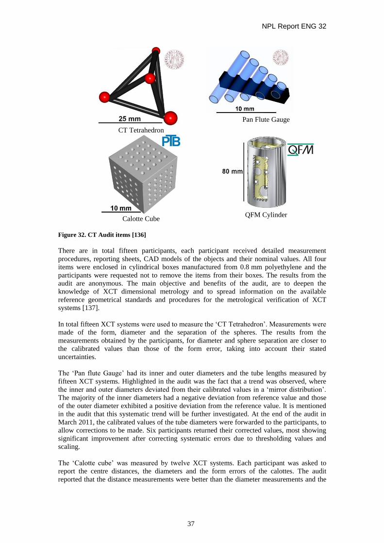
NPL Report ENG 32
37
CT Tetrahedron
Pan Flute Gauge
Calotte Cube
QFM Cylinder
Figure 32. CT Audit items [136]
There are in total fifteen participants, each participant received detailed measurement
procedures, reporting sheets, CAD models of the objects and their nominal values. All four
items were enclosed in cylindrical boxes manufactured from 0.8 mm polyethylene and the
participants were requested not to remove the items from their boxes. The results from the
audit are anonymous. The main objective and benefits of the audit, are to deepen the
knowledge of XCT dimensional metrology and to spread information on the available
reference geometrical standards and procedures for the metrological verification of XCT
systems [137].
In total fifteen XCT systems were used to measure the ‘CT Tetrahedron’. Measurements were
made of the form, diameter and the separation of the spheres. The results from the
measurements obtained by the participants, for diameter and sphere separation are closer to
the calibrated values than those of the form error, taking into account their stated
uncertainties.
The ‘Pan flute Gauge’ had its inner and outer diameters and the tube lengths measured by
fifteen XCT systems. Highlighted in the audit was the fact that a trend was observed, where
the inner and outer diameters deviated from their calibrated values in a ‘mirror distribution’.
The majority of the inner diameters had a negative deviation from reference value and those
of the outer diameter exhibited a positive deviation from the reference value. It is mentioned
in the audit that this systematic trend will be further investigated. At the end of the audit in
March 2011, the calibrated values of the tube diameters were forwarded to the participants, to
allow corrections to be made. Six participants returned their corrected values, most showing
significant improvement after correcting systematic errors due to thresholding values and
scaling.
The ‘Calotte cube’ was measured by twelve XCT systems. Each participant was asked to
report the centre distances, the diameters and the form errors of the calottes. The audit
reported that the distance measurements were better than the diameter measurements and the

NPL Report ENG 32
38
diameter measurements were better than the form error. However, the measurement results
showed that all participants overestimated the form error measurements of the calottes.
Measurements on the ‘QFM Cylinder’ were reported for eight XCT systems. This item was
found to be the most challenging item to measure, participants were asked to measure: inner
and outer diameters of cylinders, calotte diameters, sphere centre distances and diameter of
the smallest cylindrical micro structure. Due to the size of the item, not all the participants
were able to measure the complete sample. Results from one of the participants were
highlighted to show the difference in the measurement deviations of the top calottes diameters
using two different procedures [136]. One measurement was to scan the whole item, and the
other was to scan only the top calottes with the top calottes in the central plane of the
measurement field with a different magnification and thus voxel size. The results show that
the second measurements made are generally closer to the calibrated values.
The report concluded that the most accurate measurements were made on the distance
between spheres. The higher deviation measurements were on form error, and correct
measurement uncertainties were difficult to evaluate due to the numerous influences in XCT
measurements.
6.5.5 Other reference objects
Carmignato et al. [138] present the first results of a test procedure implemented for
determining the errors of indication for the length measurements using XCT systems, using a
reference object, referred to as the ‘fibre gauge’, featuring a regular array of inner and outer
cylindrical geometries (see figure 33).
Figure 33. Reference objects developed by Carmignato et al [138]
Carmignato et al. also describe a solution to the threshold value selection for the item shown
in figure 33. The optimal threshold value can be accurately evaluated by, for example, the
simultaneous measurement of the calibrated internal and external diameters of the cylinder.
The rotational symmetry allows a best-case threshold to be set.
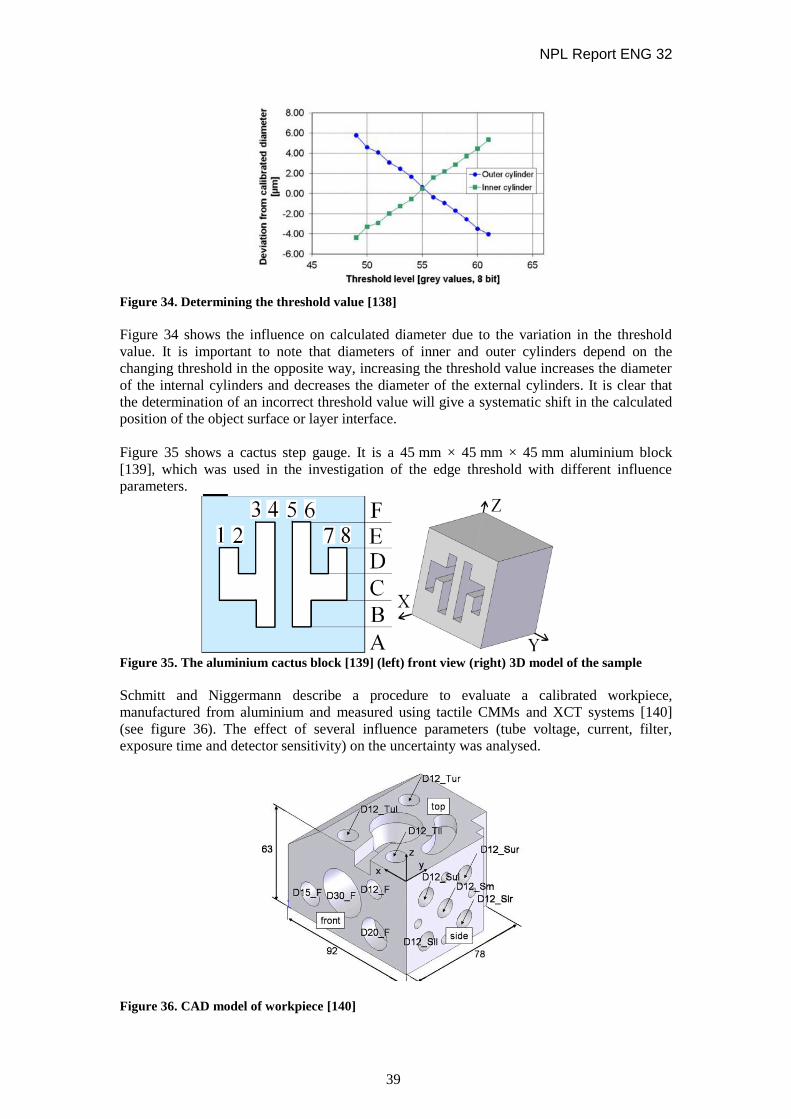
NPL Report ENG 32
39
Figure 34. Determining the threshold value [138]
Figure 34 shows the influence on calculated diameter due to the variation in the threshold
value. It is important to note that diameters of inner and outer cylinders depend on the
changing threshold in the opposite way, increasing the threshold value increases the diameter
of the internal cylinders and decreases the diameter of the external cylinders. It is clear that
the determination of an incorrect threshold value will give a systematic shift in the calculated
position of the object surface or layer interface.
Figure 35 shows a cactus step gauge. It is a 45 mm × 45 mm × 45 mm aluminium block
[139], which was used in the investigation of the edge threshold with different influence
parameters.
Figure 35. The aluminium cactus block [139] (left) front view (right) 3D model of the sample
Schmitt and Niggermann describe a procedure to evaluate a calibrated workpiece,
manufactured from aluminium and measured using tactile CMMs and XCT systems [140]
(see figure 36). The effect of several influence parameters (tube voltage, current, filter,
exposure time and detector sensitivity) on the uncertainty was analysed.
Figure 36. CAD model of workpiece [140]

NPL Report ENG 32
40
6.6 DESIGN OF REFERENCE STANDARDS
The growing use of XCT systems to quantitatively measure, as well as to inspect, the internal
and external dimensions of simple and complex parts was discussed in section 2.2. As with
any dimensional measurement technique, traceability of the measurement instrument to the
metre is essential for useful interpretation of generated data.
The VIM [34], defines metrological traceability as ‘property of a measurement result whereby
the results can be related to a reference through a documented unbroken chain of calibrations,
each contributing to the measurement uncertainty’. In the case of XCT systems, this
traceability, more often than not, is through the calibration of objects by means of tactile
CMMs. Furthermore, the document [34] continues to express, that for measurements with
more than one input quantity in the measurement model, each of the input quantity values
should itself be metrologically traceable and the calibration hierarchy involved may form a
branched structure or a network. The effort involved in establishing metrological traceability
for each input quantity value should be commensurate with its relative contribution to the
measurement result.
From section 6.5, it can be seen that there are many reference objects that are currently being
used to give traceability to XCT systems [136]. Some of these objects are being incorporated
into the standardization process [119], for example the Calotte Cube developed by PTB and
the Micro Tetrahedron developed by the University of Padova [137]. However, a few issues
need to be addressed regarding the design of reference standards:
An ideal situation would be to have an object that allows any XCT system to be
calibrated at any setting. However, XCT systems have a multitude of influence
parameters, for example, the source energy and the threshold. Unfortunately,
changing these parameters has an effect on the response of the system. To design and
build a single object that has a predictable response to these different parameters is
problematic.
Another issue that needs to be considered is the beam hardening. This effect is due to
the fact that the X-ray photons emitted from the X-ray source have a range of
energies (see figure 1). As the X-ray beam passes through the object the lower energy
photons are absorbed, which has the resultant effect of increasing the mean energy of
the beam and causes artefacts in the reconstructed image (for more information on
beam hardening, see section 5.3).
Objects consisting of multiple materials or composites can be problematic as
interfaces between different materials may become blurred or biased towards a
particular material in the event that the wrong edge threshold is used. Multiple
material objects also cause artefacts and increase noise in the analyses. In an ideal
situation, when either calibrating or verifying any XCT system, the atomic number of
the calibration object should be the same as the atomic number of the objects under
examination, so that an appropriate threshold value can be determined for the
interface under examination. An investigation into problems that can occur is given in
[23], where materials of steel, rubber and zirconium oxide have been used.
One of the advantages of XCT systems is the ability to measure, in a non-destructive
way, the internal dimensions of an object and surfaces with high aspect ratio. It is this
advantage that can become problematic when trying to achieve a traceable calibration

NPL Report ENG 32
41
chain for features with high aspect ratio, internal dimensions and positions of material
interfaces.
Due to the issues discussed above, there is no single calibration object that satisfies all the
varying parameters, such as threshold and scale, which influences the metrology of XCT
systems. There are manufacturers’ claims of the existence of such objects, but in reality they
generally only address part of the problem, such as scale.
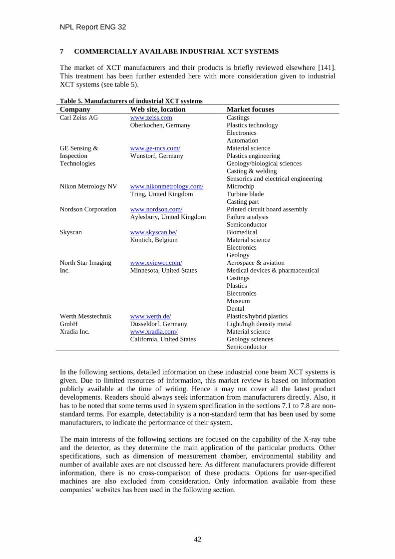
NPL Report ENG 32
42
7 COMMERCIALLY AVAILABE INDUSTRIAL XCT SYSTEMS
The market of XCT manufacturers and their products is briefly reviewed elsewhere [141].
This treatment has been further extended here with more consideration given to industrial
XCT systems (see table 5).
Table 5. Manufacturers of industrial XCT systems
Company Web site, location Market focuses Carl Zeiss AG www.zeiss.com
Oberkochen, Germany
Castings
Plastics technology
Electronics
Automation
GE Sensing &
Inspection
Technologies
www.ge-mcs.com/
Wunstorf, Germany
Material science
Plastics engineering
Geology/biological sciences
Casting & welding
Sensorics and electrical engineering
Nikon Metrology NV www.nikonmetrology.com/
Tring, United Kingdom
Microchip
Turbine blade
Casting part
Nordson Corporation
www.nordson.com/
Aylesbury, United Kingdom
Printed circuit board assembly
Failure analysis
Semiconductor
Skyscan
www.skyscan.be/
Kontich, Belgium
Biomedical
Material science
Electronics
Geology
North Star Imaging
Inc.
www.xviewct.com/
Minnesota, United States
Aerospace & aviation
Medical devices & pharmaceutical
Castings
Plastics
Electronics
Museum
Dental
Werth Messtechnik
GmbH
www.werth.de/
Düsseldorf, Germany
Plastics/hybrid plastics
Light/high density metal
Xradia Inc. www.xradia.com/
California, United States
Material science
Geology sciences
Semiconductor
In the following sections, detailed information on these industrial cone beam XCT systems is
given. Due to limited resources of information, this market review is based on information
publicly available at the time of writing. Hence it may not cover all the latest product
developments. Readers should always seek information from manufacturers directly. Also, it
has to be noted that some terms used in system specification in the sections 7.1 to 7.8 are non-
standard terms. For example, detectability is a non-standard term that has been used by some
manufacturers, to indicate the performance of their system.
The main interests of the following sections are focused on the capability of the X-ray tube
and the detector, as they determine the main application of the particular products. Other
specifications, such as dimension of measurement chamber, environmental stability and
number of available axes are not discussed here. As different manufacturers provide different
information, there is no cross-comparison of these products. Options for user-specified
machines are also excluded from consideration. Only information available from these
companies’ websites has been used in the following section.
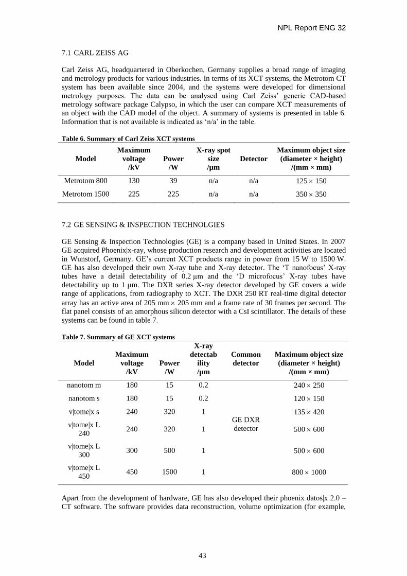
NPL Report ENG 32
43
7.1 CARL ZEISS AG
Carl Zeiss AG, headquartered in Oberkochen, Germany supplies a broad range of imaging
and metrology products for various industries. In terms of its XCT systems, the Metrotom CT
system has been available since 2004, and the systems were developed for dimensional
metrology purposes. The data can be analysed using Carl Zeiss’ generic CAD-based
metrology software package Calypso, in which the user can compare XCT measurements of
an object with the CAD model of the object. A summary of systems is presented in table 6.
Information that is not available is indicated as ‘n/a’ in the table.
Table 6. Summary of Carl Zeiss XCT systems
Model
Maximum
voltage Power
X-ray spot
size Detector
Maximum object size
(diameter × height)
/kV /W /µm /(mm × mm)
Metrotom 800 130 39 n/a n/a 125 150
Metrotom 1500 225 225 n/a n/a 350 350
7.2 GE SENSING & INSPECTION TECHNOLGIES
GE Sensing & Inspection Technologies (GE) is a company based in United States. In 2007
GE acquired Phoenix|x-ray, whose production research and development activities are located
in Wunstorf, Germany. GE’s current XCT products range in power from 15 W to 1500 W.
GE has also developed their own X-ray tube and X-ray detector. The ‘T nanofocus’ X-ray
tubes have a detail detectability of 0.2 µm and the ‘D microfocus’ X-ray tubes have
detectability up to 1 µm. The DXR series X-ray detector developed by GE covers a wide
range of applications, from radiography to XCT. The DXR 250 RT real-time digital detector
array has an active area of 205 mm 205 mm and a frame rate of 30 frames per second. The
flat panel consists of an amorphous silicon detector with a CsI scintillator. The details of these
systems can be found in table 7.
Table 7. Summary of GE XCT systems
Model
Maximum
voltage Power
X-ray
detectab
ility
Common
detector
Maximum object size
(diameter × height) /kV /W /µm /(mm × mm)
nanotom m 180 15 0.2
GE DXR
detector
240 250
nanotom s 180 15 0.2 120 150
v|tome|x s 240 320 1 135 420
v|tome|x L
240 240 320 1 500 600
v|tome|x L
300 300 500 1 500 600
v|tome|x L
450 450 1500 1 800 1000
Apart from the development of hardware, GE has also developed their phoenix datos|x 2.0 –
CT software. The software provides data reconstruction, volume optimization (for example,
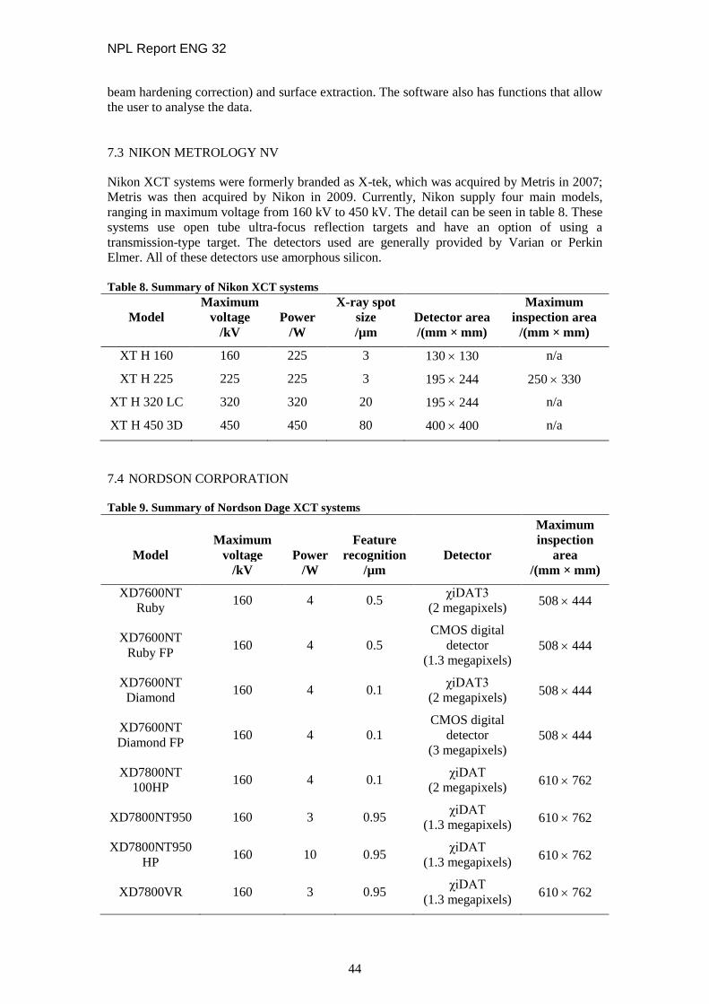
NPL Report ENG 32
44
beam hardening correction) and surface extraction. The software also has functions that allow
the user to analyse the data.
7.3 NIKON METROLOGY NV
Nikon XCT systems were formerly branded as X-tek, which was acquired by Metris in 2007;
Metris was then acquired by Nikon in 2009. Currently, Nikon supply four main models,
ranging in maximum voltage from 160 kV to 450 kV. The detail can be seen in table 8. These
systems use open tube ultra-focus reflection targets and have an option of using a
transmission-type target. The detectors used are generally provided by Varian or Perkin
Elmer. All of these detectors use amorphous silicon.
Table 8. Summary of Nikon XCT systems
Model
Maximum
voltage Power
X-ray spot
size Detector area
Maximum
inspection area /kV /W /µm /(mm × mm) /(mm × mm)
XT H 160 160 225 3 130 130 n/a
XT H 225 225 225 3 195 244 250 330
XT H 320 LC 320 320 20 195 244 n/a
XT H 450 3D 450 450 80 400 400 n/a
7.4 NORDSON CORPORATION
Table 9. Summary of Nordson Dage XCT systems
Model
Maximum
voltage Power
Feature
recognition Detector
Maximum
inspection
area
/kV /W /µm /(mm × mm)
XD7600NT
Ruby 160 4 0.5
χiDAT3
(2 megapixels) 508 444
XD7600NT
Ruby FP 160 4 0.5
CMOS digital
detector
(1.3 megapixels) 508 444
XD7600NT
Diamond 160 4 0.1
χiDAT3
(2 megapixels) 508 444
XD7600NT
Diamond FP 160 4 0.1
CMOS digital
detector
(3 megapixels) 508 444
XD7800NT
100HP 160 4 0.1
χiDAT
(2 megapixels) 610 762
XD7800NT950 160 3 0.95 χiDAT
(1.3 megapixels) 610 762
XD7800NT950
HP 160 10 0.95
χiDAT
(1.3 megapixels) 610 762
XD7800VR 160 3 0.95 χiDAT
(1.3 megapixels) 610 762

NPL Report ENG 32
45
Nordson Corporation was founded in 1954 with the headquarters in Ohio, United States. The
company acquired Dage Holdings Ltd in 2006 and the resultant operation Nordson DAGE is
headquartered in Aylesbury, UK. The XCT systems produced by Nordson DAGE use the
DAGE NT 100 sealed-transmissive, filament-free X-ray tubes. The value of feature
recognition listed in table 9 is for a tube with power below 4 W (with the exception of the
XD7800NT950HP system). The XD7600NT series systems use a 16-bit FPD with a
maximum inspection area of 508 mm 444 mm. The XD7800NT series was designed for
inspection of semiconductors and large printed circuit boards. The systems use a large FPD
with a maximum inspection area of 610 mm 762 mm. The XD7800NT 100HP system has a
frame rate of thirty frames per second. All other systems have a frame rate of twenty-five
frames per second.
7.5 SKYSCAN
SkyScan is a Belgium company that focuses on micro- and nano-XCT products. The
company was founded in 1996, with the first commercial product released a year later.
Products developed by SkyScan generally are smaller than many commercial XCT systems
on the market. For example, the size of the SkyScan 1172 system is only 1250 mm (length)
659 mm (width) 360 mm (height). The mass of SkyScan systems is generally below 500 kg.
The detail can be seen in table 10.
SkyScan has also developed its own XCT software, including NRecon, Data Viewer and
Ctvox. NRecon is the reconstruction software, Data Viewer can convert data into different
image formats and Ctvox is the visualisation software, which supports functions such as
clipping. SkyScan also provides the package CT-analyser for data analysis and CT-volume
for advanced data visualisation.
Table 10. Summary of Skyscan XCT systems
Model Voltage Power
Detail
detectability Detector
Maximum object
size (diameter ×
height)
/kV /W /µm /(mm × mm)
1172 20-100 10 0.5
11 megapixels, 12-bit
CCD fibre-optically
coupled to scintillator 50 70
1174 20-50 40 6
1.3 megapixels, 14-bit
cooled CCD with 1:6
zoom lens 30 50
1176 20-90 25 9
11 megapixels, 12-bit
CCD fibre-optically
coupled to scintillator 68 200
1178 20-65 40 80 1.3 megapixels, 12-bit
cameras 80 200
2011 20-80 n/a 0.2 1.3 megapixels, 12-bit
X-ray CCD camera 11 n/a
7.6 NORTH STAR IMAGING INC.
North Star Imaging Inc. was founded in 1986 and is headquartered in Minnesota, United
States. The company provides both open and sealed X-ray tubes. The company also

NPL Report ENG 32
46
developed software to address data acquisition, processing and archival. Details of their
systems can be found in table 11. It is also stated on the company’s website that they provide
calibrated XCT systems for dimensional metrology.
Table 11. Summary of North Star Imaging XCT systems
Model Voltage Power Focal Spot Size Detector size
Maximum
sample size
/kV /W /m /(mm × mm) /mm
ImagiX 150 n/a 5 250 250 150
X50-CT Sealed
Tube: 100,
130, 150
Open Tube:
160, 225
320, 450
n/a 1 Flat panel/
Linear array,
panel size from
100 100
to 400 400
300
X500-CT n/a 1 600
X5000-CT n/a 1 n/a.
EXPRESS-
CT n/a 1 n/a
The term ‘Maximum sample size’ used in table 11 refers to the vertical and lateral axes travel
relative to the scanning envelope.
7.7 WERTH MESSTECHINK GMBH
Werth Messtechnik GmbH was founded in 1951 in Düsseldorf, Germany. In contrast with
other XCT developers, Werth Messtechnik is focused on developing multi-sensor systems.
The first multi-sensor coordinate measuring machines with XCT was developed in 2005.
More information about their XCT systems is available in table 12. For each model, the
company allows users to choose from a range of setups.
Table 12. Summary of Werth Messtechnik XCT systems
Model
Maximum
voltage Power Resolution Detector size
Maximum object size
(diameter × height)
/kV /W /m /(mm × mm) /(mm × mm)
TomoScope
200
130
150
190
n/a 0.1 50 50
130 130 110 200
TomoCheck
200
130
150 n/a 0.1 50 50 90 200
TomoScope
HV
Compact
225 n/a 0.1 n/a 330 350
TomoScope
HV 500 225 n/a 0.1 400 400 350 500
7.8 XRADIA
Xradia was founded in 2000 and is based in California, United States. The company designs,
develops and manufactures micro- and nano-XCT systems. Apart from the systems listed in
table 13, the company also provides synchrotron X-ray microscope systems with 30 nm
resolution. However, it is unclear how the resolution has been determined. The company also
integrated a Zernike phase contrast plate to enhance the visibility of edges and interfaces

NPL Report ENG 32
47
when contrast is low. The VersaXRM-500 system also allows users to do in situ
measurements and time-dependent studies.
Table 13. Summary of Xradia XCT systems
Model
Maximum
voltage Power
Spatial
resolution Detector size Sample size
/kV /W /m /(mm × mm) /mm
MicroXCT-
200
20-90 8 1 n/a 150
MicroXCT-
400
40-150 10 1 n/a 300
Field of view
/µm
VersaXRM-
500
30-160 10 0.7 n/a n/a
UltraXRM-
L200
20-40 1200 0.05 n/a 15 to 60
7.9 UK INSTITUTIONS AND XCT RELATED WORK
XCT technology, especially with regards to industrial application, is a relatively new research
field. The recent increase in numbers of XCT systems owned by universities indicates an
increase in XCT research activities. Table 14 lists a few institutes that currently host XCT
systems. NPL is currently collaborating with the University of Southampton and the
University of Manchester. Both universities have strong research teams working on XCT and
related aspects. There are also other UK universities that own XCT facilities, such as
University of Leicester, University of Leeds and University of Nottingham, responding to a
demand for XCT in various research fields.
Table 14. Summary of UK universities that with XCT systems
Name of Institution XCT facilities
University of Southampton
(-VIS)
Nikon custom 225 kV/450 kV hutch
Nikon custom 225 kV
Nikon 160 kV benchtop
Gatan XuM/Zeiss Evo MA25
SkyScan 1176 in vivo CT
University of Manchester
(Henry Moseley X-ray Imaging Facility)
Nikon/Metris custom 320 kV bay
Nikon/Metris XTH225 kV
Xradia MicroXCT
Xradia nanoXCT
Rapiscan RTT20
University of Leicester Nikon/Metris 225 kV
University of Leeds GE/Phoenix Nanotom
University of Loughborough Nikon/Metris XT H
University of Nottingham GE/Phoenix Nanotom
University of Warwick Nikon/Metris 320 kV
University of Huddersfield Nikon XTH 225 kV

NPL Report ENG 32
48
8 CONCLUSIONS
In this report, the market trend of industrial XCT systems has been reviewed and recent
developments of both XCT hardware and software studied. Latest products on the market
have also been reviewed; the unique systematic errors associated with XCT systems discussed
and recent developments regarding the calibration and verification of XCT systems reviewed.
It is clear that the industrial XCT market is growing rapidly and there is a significant demand
to use the technology to detect faulty parts and to provide dimensional information about
measured samples. However, the development of the technology is still in its infancy.
Based on this report, there are a number of issues that need to be addressed. Using XCT as a
dimensional tool, requires the determination of the surface boundary, which is based on the
measured volumetric data. These boundaries can be significantly affected by the selection of
the threshold value, which relies heavily on the empirical knowledge of the operator. This
report has shown that there is no universal technique for predicting the correct threshold
value. It is also unclear for manufacturers, as well as end users, how to evaluate systems, as
there is no complete system verification procedure available that can be followed.
Furthermore, there are terminology issues found in the manufacturers’ literature, where terms,
such as ‘feature recognition’, ’maximum inspection area’ and ‘maximum object size’, have no
definition and are, therefore, causing confusion.
In the future, a user guide defining terminology, from both the CMM and XCT environment
would be a useful starting point. This should be followed by the development of verification
objects and surface determination methods. In parallel to this, a system verification procedure
should be developed, incorporating methods for XCT calibration based on a study of
systematic errors. All this work is required urgently to develop a traceability infrastructure for
measurements using XCT systems.
ACKNOWLEDGEMENT
This report and the underlying NPL XCT project were funded by the National Measurement
Office (NMO) Engineering Measurement and Flow Programme. The project is additionally
supported by the EPSRC Knowledge Transfer Secondments scheme, via the University of
Southampton. Many thanks are due to Professor John McBride and Professor Ian Sinclair for
providing access to -VIS XCT facilities at the University of Southampton, as well as insight
and knowledge in XCT. We would also like to thank Dr Michael McCarthy at NPL, the staff,
especially Dr Dmitry Grinev and Dr Mark Noel Mavrogordato at the University of
Southampton, Dr Fabien Leonard, Professor Phil Withers and Professor Paul Mummery at the
University of Manchester’s Henry Molesey X-ray Imaging Facility. Finally, we are grateful to
Mr Christopher Jones, Mr David Flack, Dr Andrew Yacoot and Dr Andrew Lewis, for
assistance with proofreading.

NPL Report ENG 32
49
REFERENCES
[1] Cormack A M and Hounsfield G N 1979 The Nobel Prize in Physiology or Medicine
[2] Thomas S J 1999 Relative electron density calibration of CT scanners for radiotherapy
treatment planning Brit. J. Radiol. 72 781-86
[3] Berrington de González A, Mahesh M, Kim K-P, Bhargavan M, Lewis R, Mettler F and
Land C 2009 Projected cancer risks from computed tomographic scans performed in
the United States in 2007 Arch. Intern. Med. 169 2071-77
[4] Ionising radiation Website: www.npl.co.uk/educate-explore/posters/ionising-radiation/
Accessed on 1st November 2011
[5] Feldkamp L A, Davis L C and Kress J W 1984 Practical cone-beam algorithm JOSA A:
Optics, Image Science, and Vision 1 612-19
[6] Weckenmann A, Kraemer P and Hoffmann J 2007 Manufacturing metrology - state of the
art and prospects Proc. of 9th International Symposium on Measurement and Quality
Control (IIT Madras) pp7
[7] January 2011 Computed tomography (CT) scanners: A global strategic business report
Global Industry Analysts Inc Report MCP-3321
[8] 24th March 2011 Higher standards of quality open up opportunities for X-ray inspections
systems (Frost and Sullivan)
[9] Jose S Global installed base of computed tomography (CT) scanners to reach about 60
thousand units by 2015, according to new report by global industry analysts, Inc.
Website:
www.prweb.com/releases/computed_tomography/CT_scanners/prweb8075828.htm
Accessed on 3rd August 2011
[10] Rapiscan Systems Website: www.rapiscansystems.com/ Accessed on 3rd August 2011
[11] Pollitt M 20th March 2008 How X-rays can detect cocaine or semtex in a large suitcase
The Guardian www.guardian.co.uk/technology/2008/mar/20/engineering.research
[12] (Security Media Publishing Ltd.) Website:
www.securitymiddleeast.com/news/read/american-science-and-engineering-inc-
receives-82-million-order-for-its-cargo-inspection-systems-to-secure-critical-
infrastructure-in-the-middle-east-2010-04-01 Accessed on 29 September 2011
[13] Flack D and Hannaford J 2005 Fundamental good practice in dimensional metrology
National Physical Laboratory Measurement Good Practice Guide No. 80
[14] Yang K, Kwan A L C, Miller D F and Boone J M 2006 A geometric calibration method
for cone beam CT systems Med. Phys. 33 1695-706
[15] Sun Y, Hou Y, Zhao F and Hu J 2005 A calibration method for misaligned scanner
geometry in cone-beam computed tomography Nondestructive Testing 10
[16] Holt K M 2007 Geometric calibration of third-generation computed tomography
scanners from scans of unknown objects using complementary rays Proc. of IEEE
International Conference on Image Processing (ICIP) (San Antonio)
[17] Röntgen W C 1896 On a new kind of rays Sci. 3 227-31
[18] Thomson J J 2005 Conduction of electricity through gases (Wexford College Press)
[19] Young H D, Freedman R A, Sandin T R and Ford A L 1999 Sears and Zemansky's
university physics (10th Edition) (Addison-Wesley)
[20] 2007 Industrial radiography image forming techniques (General Electric Company)
GEIT 30158EN
[21] Maur F W 2007 Lastest developments in X-ray microscopy Proc. of International
Workshop on Imaging NDE (Kalpakkam, India)
[22] X-ray tube basics Website: h2g2.com/dna/h2g2/A14017943 Accessed on 1st October
2011
[23] Kruth J P, Bartscher M, Carmignato S, Schmitt R, De Chifffre L and Weckenmann A
2011 Computed tomography for dimensional metrology Ann. CIRP 60 821-42
[24] Daneke N and Schanklies B October 2004 From microfocus to nanofocus X-ray
inspection OnBoard Technology 42-44
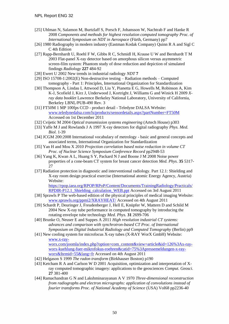
NPL Report ENG 32
50
[25] Uhlman N, Salamon M, Burtzlaff S, Porsch F, Johansson W, Nachtrab F and Hanke R
2008 Components and methods for highest resolution computed tomography Proc. of
International Symposium on NDT in Aerospace (Fürth, Germany) pp7
[26] 1980 Radiography in modern industry (Eastman Kodak Company) Quinn R A and Sigl C
C 4th Edition
[27] Rapp-Bernhardt U, Roehl F W, Gibbs R C, Schmidl H, Krause U W and Bernhardt T M
2003 Flat-panel X-ray detector based on amorphous silicon versus asymmetric
screen-film system: Phantom study of dose reduction and depiction of simulated
findings Radiology 227 484-92
[28] Ewert U 2002 New trends in industrial radiology NDT 7
[29] ISO 15708-1:2002(E) Non-destructive testing – Radiation methods – Computed
tomography - Part 1: Principles, International Organization for Standardization
[30] Thompson A, Lindau I, Attwood D, Liu Y, Pianetta E G, Howells M, Robinson A, Kim
K-J, Scofield J, Kirz J, Underwood J, Kortright J, Williams G and Winick H 2009 X-
ray data booklet Lawrence Berkeley National Laboratory, University of California,
Berkeley LBNL/PUB-490 Rev. 3
[31] FT50M 1 MP 100fps CCD - product detail - Teledyne DALSA Website:
www.teledynedalsa.com/ls/products/sensordetails.aspx?partNumber=FT50M
Accessed on 1st December 2011
[32] Cvijetic M 2004 Optical transmission systems engineering (Artech House) p303
[33] Yaffe M J and Rowlands J A 1997 X-ray detectors for digital radiography Phys. Med.
Biol. 1-39
[34] JCGM 200:2008 International vocabulary of metrology - basic and general concepts and
associated terms, International Organization for Standardization
[35] Yan H and Mou X 2010 Projection correlation based noise reduction in volume CT
Proc. of Nuclear Science Symposium Conference Record pp2948-53
[36] Yang K, Kwan A L, Huang S Y, Packard N J and Boone J M 2008 Noise power
properties of a cone-beam CT system for breast cancer detection Med. Phys. 35 5317-
27
[37] Radiation protection in diagnostic and interventional radiology. Part 12.1: Shielding and
X-ray room design practical exercise (International atomic Energy Agency, Austria)
Website:
https://rpop.iaea.org/RPOP/RPoP/Content/Documents/TrainingRadiology/Practicals/
RPDIR-P12.1_Shielding_calculation_WEB.ppt Accessed on 3rd August 2011
[38] Sprawls P The web-based edition of the physical principles of medical imaging Website:
www.sprawls.org/ppmi2/XRAYHEAT/ Accessed on 4th August 2011
[39] Schardt P, Deuringer J, Freudenberger J, Hell E, Knüpfer W, Mattern D and Schild M
2004 New X-ray tube performance in computed tomography by introducing the
rotating envelope tube technology Med. Phys. 31 2699-706
[40] Brunke O, Neuser E and Suppes A 2011 High resolution industrial CT systems:
advances and comparison with synchrotron-based CT Proc. of International
Symposium on Digital Industrial Radiology and Computed Tomography (Berlin) pp9
[41] New cooling system for microfocus X-ray tubes (X-RAY WorX GmbH) Website:
www.x-ray-
worx.com/joomla/index.php?option=com_content&view=article&id=126%3Ax-ray-
worx-kuehlung-fuer-mikrofokus-roehren&catid=75%3Apressemeldungen-x-ray-
worx&Itemid=55&lang=fr Accessed on 4th August 2011
[42] Helgason S 1999 The radon transform (Birkhauser Boston) p190
[43] Ketcham R A and Carlson W D 2001 Acquisition, optimization and interpretation of X-
ray computed tomographic imagery: applications to the geosciences Comput. Geosci.
27 381-400
[44] Ramachandran G N and Lakshminarayanan A V 1970 Three-dimensional reconstruction
from radiographs and electron micrographs: application of convolutions instead of
fourier transforms Proc. of National Academy of Science (USA) Vol68 pp2236-40
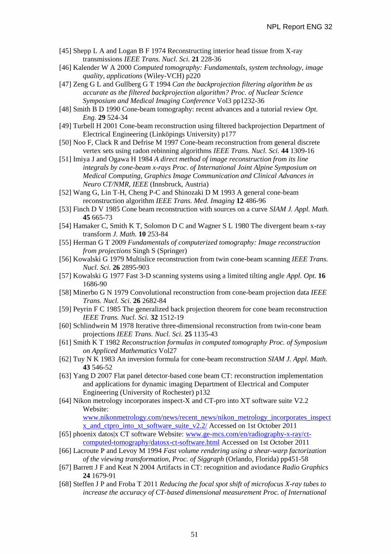
NPL Report ENG 32
51
[45] Shepp L A and Logan B F 1974 Reconstructing interior head tissue from X-ray
transmissions IEEE Trans. Nucl. Sci. 21 228-36
[46] Kalender W A 2000 Computed tomography: Fundamentals, system technology, image
quality, applications (Wiley-VCH) p220
[47] Zeng G L and Gullberg G T 1994 Can the backprojection filtering algorithm be as
accurate as the filtered backprojection algorithm? Proc. of Nuclear Science
Symposium and Medical Imaging Conference Vol3 pp1232-36
[48] Smith B D 1990 Cone-beam tomography: recent advances and a tutorial review Opt.
Eng. 29 524-34
[49] Turbell H 2001 Cone-beam reconstruction using filtered backprojection Department of
Electrical Engineering (Linköpings University) p177
[50] Noo F, Clack R and Defrise M 1997 Cone-beam reconstruction from general discrete
vertex sets using radon rebinning algorithms IEEE Trans. Nucl. Sci. 44 1309-16
[51] Imiya J and Ogawa H 1984 A direct method of image reconstruction from its line
integrals by cone-beam x-rays Proc. of International Joint Alpine Symposium on
Medical Computing, Graphics Image Communication and Clinical Advances in
Neuro CT/NMR, IEEE (Innsbruck, Austria)
[52] Wang G, Lin T-H, Cheng P-C and Shinozaki D M 1993 A general cone-beam
reconstruction algorithm IEEE Trans. Med. Imaging 12 486-96
[53] Finch D V 1985 Cone beam reconstruction with sources on a curve SIAM J. Appl. Math.
45 665-73
[54] Hamaker C, Smith K T, Solomon D C and Wagner S L 1980 The divergent beam x-ray
transform J. Math. 10 253-84
[55] Herman G T 2009 Fundamentals of computerized tomography: Image reconstruction
from projections Singh S (Springer)
[56] Kowalski G 1979 Multislice reconstruction from twin cone-beam scanning IEEE Trans.
Nucl. Sci. 26 2895-903
[57] Kowalski G 1977 Fast 3-D scanning systems using a limited tilting angle Appl. Opt. 16
1686-90
[58] Minerbo G N 1979 Convolutional reconstruction from cone-beam projection data IEEE
Trans. Nucl. Sci. 26 2682-84
[59] Peyrin F C 1985 The generalized back projection theorem for cone beam reconstruction
IEEE Trans. Nucl. Sci. 32 1512-19
[60] Schlindwein M 1978 Iterative three-dimensional reconstruction from twin-cone beam
projections IEEE Trans. Nucl. Sci. 25 1135-43
[61] Smith K T 1982 Reconstruction formulas in computed tomography Proc. of Symposium
on Appliced Mathematics Vol27
[62] Tuy N K 1983 An inversion formula for cone-beam reconstruction SIAM J. Appl. Math.
43 546-52
[63] Yang D 2007 Flat panel detector-based cone beam CT: reconstruction implementation
and applications for dynamic imaging Department of Electrical and Computer
Engineering (University of Rochester) p132
[64] Nikon metrology incorporates inspect-X and CT-pro into XT software suite V2.2
Website:
www.nikonmetrology.com/news/recent_news/nikon_metrology_incorporates_inspect
x_and_ctpro_into_xt_software_suite_v2.2/ Accessed on 1st October 2011
[65] phoenix datos|x CT software Website: www.ge-mcs.com/en/radiography-x-ray/ct-
computed-tomography/datosx-ct-software.html Accessed on 1st October 2011
[66] Lacroute P and Levoy M 1994 Fast volume rendering using a shear-warp factorization
of the viewing transformation, Proc. of Siggraph (Orlando, Florida) pp451-58
[67] Barrett J F and Keat N 2004 Artifacts in CT: recognition and aviodance Radio Graphics
24 1679-91
[68] Steffen J P and Froba T 2011 Reducing the focal spot shift of microfocus X-ray tubes to
increase the accuracy of CT-based dimensional measurement Proc. of International

NPL Report ENG 32
52
Symposium on Digital Industrial Radiology and Computed Tomography (Berlin,
Germany)
[69] Vogeler F, Verheecke W, Voet A, Kruth J-P and Dewulf W 2011 Positional stability of
2D X-ray images for computed tomography Proc. of International Symposium on
Digital Industrial Radiology and Computed Tomography (Berlin, Germany)
[70] Sijbers J and Postnov A 2004 Reduction of ring artefacts in high resolution micro-CT
reconstructions Phys. Med. Biol. 49 247-53
[71] Bock R, Hoppe S, Scherl H and Hornegger J 2007 Beam hardening correction with an
iterative scheme using an exact backward projector and a polychromatic forward
projector Proc. of Bildverarbeitung für die Medizin (Munich, Germany: Springer)
pp46-50
[72] Ramakrishna K, Muralidhar K and Munshi P 2006 Beam-hardening in simulated X-ray
tomography NDT & E Int. 39 449-57
[73] Van Gompel G, Van Slambrouck K, Defrise M, Batenburg K J, de Mey J, Sijbers J and
Nuyts J 2011 Iterative correction of beam hardening artifacts in CT Med. Phys. 38
S36-49
[74] Herman G T 1979 Demonstration of beam hardening correction in computed-
tomography of the head J. Comput. Assisted Tomogr. 3 373-78
[75] Krumm M, Kasperl S and Franz M 2010 Beam hardening correction of multi-material
objects Proc. of 10th European Conference on Non-Destructive Testing (Moskau)
pp7
[76] Pettersson H, Allison D, von Schulthess G K and Smith H-J 1998 The encyclopaedia of
medical imaging - Volume I: Physics, techniques and procedures
[77] Alvarez R E and Macovski A 1976 Energy-selective reconstruction in X-ray
computerized tomography Phys. Med. Biol. 21 733-44
[78] Seibert J A and Boone J M 2005 X-ray imaging physics for nuclear medicine
technologists. Part 2: X-ray interactions and image formation J. Nucl. Med. Technol.
33 3-18
[79] Smith C R, Holt K, Bischoff U, Georgi B, Hansen F and Jeltsch F 2007 Application of
450 kV computed tomography to engine blocks with steel liners Mater. Eval. 65 458-
61
[80] Popilock R, Sandrasagaren K, Harris L and Kaser K A 2008 CT artifact recongnition for
the nuclear technologist J. Nucl. Med. Technol. 36 279-81
[81] Van de Casteele E, Van Dyck D, Sijbers J and Raman E 2004 A model-based correction
method for beam hardening artefacts in X-ray microtomography J. X-ray Sci.
Technol. 12 53-57
[82] Kachelriess M, Sourbelle K and Kalender W 2006 Empirical cupping correction: A first-
order raw data precorrection for cone-beam computed tomography Med. Phys. 33
1269-74
[83] Zhang L, Gao H, Li S, Chen Z and Xing Y 2006 Cupping artifacts analysis and
correction for a FPD-based cone-beam CT Proc. of SPIE (San Jose, CA, USA)
Vol6065
[84] Lee R D Common image artifacts in cone beam CT Website:
www.aadmrt.com/currents/lee_summer_08_print.htm Accessed on 1st October 2011
[85] Balter S, Bassano D, McCullough E C, Payne J T and Rothenberg L 1977 Phantoms for
performance evaluation and quality assurance of CT scanners American Association
of Physicists in Medicine Report No 1
[86] Leach R K 2010 Fundamental principles of engineering nanometrology (Elsevier)
[87] ISO 9000:2005 Quality management systems — Fundamentals and vocabulary,
International Organization for Standardization
[88] Wein W, Ladikos A and Baumgartner A 2011 Self-calibration of geometric and
radiometric parameters for cone-beam computed tomography Proc. of 11th
International Meeting on Fully Three-Dimensional Image Reconstruction in
Radiology and Nuclear Medicine (Munchen, Germany) pp4
NPL Report ENG 32
53
[89] Kyriakou Y, Prell D, Kalender W A and Kachelrieß M 2010 Empirical beam hardening
correction for CT Med. Phys. 37 5179-87
[90] Grimmer R, Maaß C and Kachelrieß M 2009 A new method for cupping and scatter
precorrection for flat detector CT Proc. of Nuclear Science Symposium and Medical
Imaging Conference, IEEE (Orlando, Florida, USA) pp3517-22
[91] Zhu S, Tian J, Yan G, Qin C and Liu J 2009 Cone beam micro-CT system for small
animal imaging and performance evaluation Int. J. Biomed. Imaging 2009 9
[92] Romanov A Y 2004 Measurement of the parameters of the focal spot of an X-ray tube
using Kumakhov optics Meas. Tech. 47 670-74
[93] Robinson A and Grimshaw G M 1975 Measurement of the focal spot size of diagnostic
X-ray tubes—a comparison of pinhole and resolution methods Br. J. Radiol. 48 572-
80
[94] Chen Q, Chen Y, Chen M, Chao E, Sterpin E and Lu W 2011 A slit method to determine
the focal spot size and shape of TomoTherapy system Med. Phys. 38 2841-49
[95] Russo P and Mettivier G 2011 Method for measuring the focal spot size of an x-ray tube
using a coded aperture mask and a digital detector Med. Phys. 38
[96] BS EN 12543-5:1999 Non-destructive testing. Characteristics of focal spots in industrial
X-ray systems for use in non-destructive testing. Measurement of the effective focal
spot size of mini and micro focus X-ray tubes, British Standards Institution
[97] Salamon M, Hanke R, Krüger P, Sukowski F, Uhlmann N and Voland V 2008
Comparison of different methods for determining the size of a focal spot of
microfocus X-ray tubes Nucl. Instrum. Meth. A 591 54-58
[98] Cho Y, Siewerdsen J H and Jaffray D A 2005 Accurate technique for complete
geometric calibration of cone-beam computed tomography systems Med, Phys. 32
968-83
[99] Panetta D, Belcari N, Guerra A D and Moehrs S 2008 An optimization-based method for
geometrical calibration in cone-beam CT without dedicated phantoms Phys. Med.
Biol. 53 3841-61
[100] Chaney E L and Hendee W R 1974 Effects of X-ray tube current and voltage on
effective focalspot size Med. Phys. 1 141-47
[101] Gunnarsson M 1995 Evaluation of a new method for focal spot size measurements - A
study on mammography X-ray tubes Radiation Physics Department, University of
Gothenburg (Master Thesis) p33
[102] LaMarr B, Bautz M, Kissel S, Prigozhin G, Hayashida K, Tsuru T and Matsumoto H
2004 Ground calibration of X-ray CCD detectors with charge injection for the X-ray
imaging spectrometer on Astro-E2 Proc. of SPIE Vol15501 pp385-91
[103] CBCT electron density and image quality phantom (Computer Imaging Reference
Systems, Inc) Website: www.imagingequipment.co.uk/downloadfile/742 Accessed on
3rd August 2011
[104] ISO 10360-1:2000 Geometrical product specifications (GPS) — Acceptance and
reverification tests for coordinate measuring machines (CMM) —Part 1: Vocabulary,
International Organization for Standardization
[105] ISO 10360-2:2009 Geometrical product specifications (GPS) — Acceptance and
reverification tests for coordinate measuring machines (CMM) —Part 2: CMMs used
for measuring linear dimensions, International Organization for Standardization
[106] ISO 10360-3:2000 Geometrical product specifications (GPS) — Acceptance and
reverification tests for coordinate measuring machines (CMM) -- Part 3: CMMs with
the axis of a rotary table as the fourth axis, International Organization for
Standardization
[107] ISO 10360-4:2000 Geometrical product specifications (GPS) — Acceptance and
reverification tests for coordinate measuring machines (CMM) —Part 4: CMMs used
in scanning measuring mode, International Organization for Standardization
[108] ISO 10360-5:2010 Geometrical products specification (GPS) — Acceptance and
reverification tests for coordinate measuring machines (CMM) — Part 5: CMMs

NPL Report ENG 32
54
using single and multiple stylus probing systems, International Organization for
Standardization
[109] ISO 10360-6:2001 Geometrical product specifications (GPS) — Acceptance and
reverification tests for coordinate measuring machines (CMM) —Part 6: Estimation
of errors in computing Gaussian associated features, International Organization for
Standardization
[110] ISO 10360-7:2011 Geometrical product specifications (GPS) — Acceptance and
reverification tests for coordinate measuring machines (CMM) -- Part 7: CMMs
equipped with imaging probing systems, International Organization for
Standardization
[111] Flack D 2011 CMM verification Measurement Good Practice Guide No. 42
[112] ISO 15708-2:2002(E) Non-destructive testing – Radiation methods – Computed
tomography – Part 2: Examination practices, International Organization for
Standardization
[113] ISO/TC 213 N 1346 Geometrical product specification (GPS) - Acceptance and and
reverification tests for coordinate measuring machines (CMM) - Computed
tomography, International Organization for Standardization
[114] ASTM E1695 - 95(2006)e1 Standard test method for measurement of computed
tomography (CT) system performance, ASTM International
[115] ASTM E 1441 - 00 Standard guide for computed tomography (CT) imaging, ASTM
International
[116] ASTM E 1570 - 11 Standard practice for computed tomography (CT) examination,
ASTM International
[117] VDI/VDE 2630 Part 1.1:2009 Computed tomography in dimensional measurement -
Basics and definitions, Institute for Innovation and Technology
[118] VDI/VDE 2630 Part 1.2:2010 Computed tomography in dimensional measurement -
Influencing variables on measurement results and recommendations for computed
tomography dimensional measurements, Institute for Innovation and Technology
[119] VDI/VDE 2630 Part 1.3:2011 Computed tomography in dimensional measurement -
Guideline for the application of DIN EN ISO 10360 for coordinate measuring
machines with CT-sensors, Institute for Innovation and Technology
[120] Ronchi V 1961 Resolving power of calculated and detected images J. Opt. Soc. Am. 51
458-60
[121] den Dekker A J and van den Bos A 1997 Resolution: a survey JOSA A: Optics, Image
Science, and Vision 14 547-57
[122] Leach R K 2011 Optical measurement of surface topography (Springer) p323
[123] Yester M W and Barnes G T 1977 Geometrical limitations of computed tomography
(CT) scanner resolution Proc. of Applications of Optical instrumentation in medicine,
SPIE Vol127 pp296-303
[124] Sharma K S, Seshadri S, Feser M and Wang G 2010 Accurate resolution measurement
for X-ray micro-CT systems Proc. of X-Ray Microscopy (Chicago)
[125] Grimmer R, Krause J, Karolczak M, Lapp R and Kachelrib M 2008 Assessment of
spatial resolution in CT Proc. of Nuclear Science Symposium and Medical Imaging
Conference (Dresden, Germany) pp5562 - 66
[126] Staude A and Goebbels J 2011 Determining the spatial resolution in compute
tomography – comparison of MTF and line-pair structures Proc. of International
Symposium on Digital Industrial Radiology and Computed Tomography (Berlin,
Germany) pp9
[127] prEN 16016-3:2009: E Non destructive testing - Radiation methods - Computed
tomography - Part 3: Operation and interpretation, Austrian Standards Institute
[128] Hanson K M 1981 Radiology of the skull and brain, Vol. 5: Technical aspects of
computed tomography 113 Noise and contrast discrimination in computed
tomography Newton T H and Potts D G
[129] Lida H, Sasaki H, Inoue H, Kanno I, Miura S, Okuyama D and Uemura K 1986 A
simulation study to evaluate the statistical noise and spatial resolution in image

NPL Report ENG 32
55
reconstruction of emission computed tomography--with respect to the optimization of
the filter function in the convolution integral Radioisotopes 35 589-94
[130] Bartscher M, Neukamm M, Hilpert U, Neuschaefer-Rube U, Härtig F, Kniel K, Ehrig
K, Staude A and Goebbels J 2010 Achieving traceability of industrial computed
tomography Key. Eng. Mater. 437 79-83
[131] Neuschaefer-Rube U, Neugebauer M, Ehrig W, Bartscher M and Hilpert U 2008 Tactile
and optical microsensors: test procedures and standards Meas. Sci. Technol. 19
[132] Bartscher M, Hilpert U, Goebbels J and Weidemann G 2007 Enhancement and proof of
accuracy of industrial computed tomography (CT) measurements Ann. CIRP 56 495-
98
[133] Bartscher M, Neukamm M, Koch M, Neuschaefer-Rube U, Staude A, Goebbels J, Ehrig
K, Kuhn C and Deffner A 2010 Performance assessment of geometry measurements
with micro-CT using a dismountable work-piece-near reference standard Proc. of
10th European Conference on Non-Destructive Testing (Moscow: NDT)
[134] Lettenbauer H, Weiss D and Georgi B 17th November 2009 Verification of the
accuracy of computed tomography: systems for measuring 3-D technology Quality
Digest Magazine www.qualitydigest.com/inside/metrology-article/verification-
accuracy-computed-tomography.html#
[135] CT Audit:Interlaboratory comparison of computed tomography systems for dimensional
metrology (Laboratory of Industrial and Geometrical Metrology, University of
Padova) Website: static.gest.unipd.it/~carmignato/ct-audit/index.htm Accessed on 3rd
August 2011
[136] Pierobon A and Carmignato S 2011 Preliminary results of the ‘CT Audit’ project: First
international intercomparison of computed tomography systems for dimensional
metrology Proc. of International Symposium on Digital Industrial Radiology and
Computed Tomography (Berlin, Germany) pp8
[137] Carmignato S, Pierobon A and Savio E 2011 CT audit - interlaboratory comparison of
computed tomography systems for dimensional metrology (University of Padova)
[138] Carmignato S, Dreossi D, Mancini L, Marinello F, Tromba G and Savio E 2009 Testing
of X-ray microtomography systems using a traceable geometrical standard Meas. Sci.
Technol. 20 084021-28
[139] Kiekens K, Welkenhuyzen F, Tan Y, Bleys P, Voet A, Kruth J-P and Dewulf W 2011 A
test object with parallel grooves for calibration and accuracy assessment of industrial
computed tomography (CT) metrology Meas. Sci. Technol. 22 115502-09
[140] Schmitt R and Niggemann C 2010 Uncertainty in measurement for x-ray-computed
tomography using calibrated work pieces Meas. Sci. Technol. 21 054008-17
[141] Schambach S J, Bag S, Schilling L, Groden C and Brockmann M A 2010 Application
of micro-CT in small animal imaging Methods 50 2-13