- 1 -

STUDIES ON EFFECTS OF PERIODIC WAKE PASSING UPON A BLADE LEADING EDGE SEPARATION BUBBLE: TRANSITIONAL BEHAVIORS OF SEPARATED BOUNDARY LAYER

K. Funazaki1, K. Yamada1 and Y. Kato2

1 Department of Mechanical Engineering

Iwate University

3-5, Ueda 4, Morioka 020-8551, Japan

Phone/Fax: +81-19-621-6244, E-mail: funazaki@iwate-u.ac.jp2 Ishikawajima-Harima Heavy Industries Co.

ABSTRACTThis paper describes an experimental investigation on aerody-

namic interaction between incoming periodic wakes and leading edgeseparation bubble on a compressor or turbine blade, using a scaledleading edge model that consists of a semi-circular leading edge andtwo flat-plates. Cylindrical bars of the wake generator produce theperiodic wakes in front of the test model. The study aims at deepen-ing the knowledge on how and to what extent the periodic wakepassing suppresses the leading edge separation bubble. Special at-tention is paid to the transitional behaviors of the separated bound-ary layers. Hot-wire probe measurements are then executed underfive different flow conditions to examine effects of Reynolds num-ber, Strouhal number, direction of the bar movement and incidenceof the test model against the incoming flow. The measurements re-veal that the wake moving over the separation bubble does not di-rectly suppress the separation bubble. Instead, wake-induced turbu-lence spots and the subsequent calmed regions have dominant im-pacts on the separation bubble suppression for the all test cases.Numerical simulations are also attempted to grasp an idea how theincoming wakes interact with the separation bubble. A distinct dif-ference is also observed in terms of the bubble suppressing effect bythe wakes when the direction of the bar movement is altered.

INTRODUCTIONRecent studies of great numbers have investigated the interac-

tion between periodically incoming wakes and separation bubble oncompressor or LP (low-pressure) turbine blades, aiming at the ac-quisition of detailed information on the behaviors of the wake-af-fected separation bubble. For example, Halstead et al. (1995a-d) com-prehensively reported on ensemble-averaged quasi-wall shear stresson compressor or turbine blades to elucidate the interaction betweenupstream wakes-the blade boundary layer using test rigs for com-pressors and turbines. Cumptsy et al. (1995) investigated wake-af-fected boundary layers accompanied with separation bubble on acompressor cascade. Schulte and Hodson (1994), Kaszeta, Simonand Ashpis (2001), examined wake-separation bubble interactionusing linear turbine cascades and moving bars, aiming at the clarifi-cation of favorable effects of the wake passing upon the separationin terms of the profile loss reduction.

IGTC2003Tokyo TS-069

Copyright@2003 by GTSJ

In contrast to those enriched knowledge concerning the separa-tion bubble on the blade suction surface, there still be less informa-tion on the interaction between the incoming wakes and leading edgeseparation bubble on a compressor or a turbine blade. Except for apioneering effort done by Paxson and Mayle (1990), few attentionwas paid to the leading edge flow fields with separation bubble.Recently, Brear et al. (2001) examined flow separation occurringjust behind the blade leading edge on the pressure surface of LPturbine cascade subjected to the periodic wakes from the movingbars. Flow visualizations and aerodynamic loss measurements weremade in their study, showing that the shear layer was found to beslightly affected by the wake passing or increased free-stream tur-bulence. Funazaki and Kato (2002), using a simple scaled leadingedge model of compressor blade and the moving bar mechanism,executed detailed measurements of the separated boundary layer onthe test model affected by the periodic wake passing. Similarly, asimplified flat-plate model experiment was made by Ottavy et al.(2002), followed by Chun and Sung (2002).

The present study is an extended version of the previous study(Funazaki and Kato, 2002) using the almost similar test facility. Fo-cus is on the clarification of the wake-passing effects on transitionalbehaviors of the separated boundary layers occurring near the lead-ing edge of the test model subjected to various flow conditions. Thenone can finally observe the how and to what extent important flowparameters, such as direction of the bar movement, wake-passingStrouhal number, inlet Reynolds number and incident of the model,altered the transitional characteristics of the wake-affected transi-tional boundary layers. Special attention is paid to the emergence ofwake-induced turbulence spots, which was already reported byFunazaki and Kato (2002) with less quantitative discussion, though.Numerical simulation is also made to provide an idea on how theincoming periodic wakes interact with the separation bubble.

NOMENCLATUREd : bar diameterfbp : bar-passing frequency(=U pb )i : incidenceN : number of data segments for ensemble-averagingp : bar pitch (= 0.3175 m)R : radius of the leading edge of the test model

Manuscript received on April 29, 2003

Proceedings of the International Gas Turbine Congress 2003 TokyoNovember 2-7, 2003

- 2 -

Re : Reynolds number (= U Rin ν )t : timeT : bar-passing period (= p Ub )

T * : time length of data segment for ensemble averaging

Tu* : ensemble-averaged turbulence intensityUb : bar speedUin : inlet velocityUmax : maximum velocity attained near the surfaceU ref : reference velocity measured at y = 50mmuk , u*, u : raw velocity data, ensemble-averaged velocity and time-

averaged velocityxs : distance along the surface from the leading edgeY : vertical distance from the center line of the test modely : vertical distance from the test model surfaceymax : height where the maximum velocity Umax appearedν : kinematic viscosityδ1

* ,δ2* : ensemble-averaged displacement and momentum

thickness

EXPERIMENTAL APPARATUSTest Facility

Test facility used in this study was almost the same as that in theprevious study [15]. Figure 1 shows the experimental setup. Thewake generator, which was attached to the exit of the contractionnozzle, consisted of two long timing belts, four geared pulleys andstainless-steel bars. The bars of 6mm diameter were tightly fixed tothe belts horizontally using connecting profiles glued on both of thebelts. The pitch of the profiles was 63.5 mm and the profile numberwas 50. The induction motor drove the belts at a speed ranging from4.5 m/s to 7.5 m/s and the direction of the bar movement was revers-

ible. The distance between the upstream and downstream loci of thebars was about 300 mm.

Figure 2 depicts the test model that was in the test duct. Themodel, with a semi-circular leading edge of 100 mm radius (= R )and two flat plates, was 900 mm long and 280 mm wide. Two thinfences were attached to the test model surface near the both sidewalls of the duct to minimize side-wall contamination. The modelwas distanced by 245 mm from the downstream locus of the movingbars. A Pitot tube monitored the inlet velocity in front of the testsection. The test model could be tilted to change incidence againstthe inlet flow.

Test ConditionsTable 1 is the test conditions of this study. Test Case 1 was a

baseline experiment, where the inlet velocityUin was 10 m/s andthe bars moved upwards just in front of the model at a speed of 6 m/s. Reynolds number Re based on the radius of the model leadingedge and the inlet velocity was 6 5 104. × . Test Case 2 aimed at clari-fication on how differently the wakes generated from the bar mov-ing downwards affected the separation bubble in comparison withthe results of Test Case 1. Caution might be necessary in interpreta-tion of the results of Test Case 3 because the wake characteristicsmight have altered due to the change in relative inlet velocity againstthe bar. Test Case 4, where the bar speed increased by 25% from thebaseline experiment, was for examining the effect of wake-passingfrequency or Strouhal number. Reynolds number effects were in-vestigated in Test Case 4, where the bar speed was decreased so asto keep the Strouhal number the same as that of Test Case 1. In TestCase 5 the model was tilted as shown in Figure 3 to change theincidence from 0o to 5o .

Figure 1 Test apparatus with wake generator

Figure 2 Test model and two hot-wire probes

Test Model

Flow

245

Hot-Wire Probe for Mea-surement

Hot-Wire Probe forDetecting Wakes

30

Upward(Reverse)

Downward(Normal)

xs

y

R i

Wake Generator

TestModel

Settling Chamber

Blower

ContractionNozzle

Gear Pulley

Support

Timing Belt

Profile

Tensioner

Induction Motor

Cylindrical Bar

Flow Direction

300

1000

Gear Pulley

Rear View Side View

Figure 3 Test model and two hot-wire probes

Downstream Wake

Triggered Point Triggered Point

Data segment

T* T* T*

- 3 -

able for each of the realizations. Ensemble-averaged velocity u*

was then calculated from the extracted 50 data segments as follows;

u x y tN

u x y t Nkk

N* , ; , ;( ) = ( ) =

=∑

150

1, . (1)

The count of the segments for this ensemble-averaging was rathersmall in comparison with those commonly used in any other stud-ies, however, as discussed later, N = 50 was found to be almost asatisfying count, at least in the present case.

Ensemble-averaged velocity fluctuation ∆u x y tk* , ;( ) was also

evaluated by

∆u x y t u x y t u x yk k* *, ; , ; ,( ) = ( )− ( ) , (2)

where u x y,( ) was time-averaged velocity calculated by

u x yT

u x y t dtt

t T

, , ;*( ) = ( )+∫

1

0

0

. (3)

Ensemble-averaged turbulence intensity was also defined as,

Tu x y tN

u Ukk

N* *, ;( ) =

− =∑

1

1

2

1∆ ref , (4)

where U ref was reference velocity, and in this case time-averagedvelocity obtained at the upper limit of the measurement region y R= 0.5 was adopted as the reference velocity.

The following expressions were employed to calculate bound-ary layer integral parameters using the ensemble-averaged velocity;

δ10

1**

max;

;

;

max ;

x tu x t

U x tdy

y x t

( ) = −( )

( )

( )∫ , (5)

δ20

1**

max

*

max;

;

;

;

;

max ;

x tu x t

U x t

u x t

U x tdy

y x t

( ) =( )

( )−

( )( )

( )∫ , (6)

where δ1* and δ2

* were ensemble-averaged displacement thicknessand momentum thickness, respectively. Note that y x tmax ,( ) wasthe location where the velocity reached the maximum U x tmax ,( ) inthe vicinity of the test model surface and regarded as the boundarylayer thickness in this study.

Uncertainty AnalysisSince the calibration curve of a 4-th order polynomial matched

the velocity data measured with a pneumatic probe quite well, a majorcontributor to the uncertainty in the velocity data acquired by thehot-wire probe was the error in the pneumatic probe measurement.This error, mainly depending on the accuracy of the pressure trans-ducer used, was estimated to be about ±0.6 [m/s].

Besides, the convergence rate of the ensemble-averaging surelyhad a serious impact on the uncertainty of the resultant velocity.Figure 4 shows an example of the convergence histories of the en-semble averaging with the increase of N , using the experimentalraw data at x Rs = 1.695 and y R = 0.05. It seems that the en-semble-averaged velocity calculated from more than 50 velocitysegments almost got converged, with the average residual less than0.05 [m/s].

Single hot-wire probes cannot detect reversed flow without anymanipulations, so that the present measurements inevitably sufferedfrom the under- or overestimations of the boundary layer integralparameters given by Eqs. (5) and (6). Detailed investigations re-vealed that in the no wake case, which was the worst case, the dis-placement thickness was underestimated by 7% and the momentumthicknesses were overestimated by 50%, respectively, at the posi-tion where the reversed flow became active most.

The measurement region extended from x Rs = 0.96 (55o fromthe center line) to x Rs = 4.57 in the streamwise direction and fromy R = 0 3 10 2. × − to y R =0.5 in the vertical direction.

Data AcquisitionFigure 2 clearly indicates that the bars passed across the main

flow twice in one revolution of the belts at the different streamwisepositions. This inevitably generated two different types of the wakes,‘upstream wakes’ at the far upstream of the test model and ‘down-stream wakes’ near the model. Since this study intended to investi-gate only the effect of the ‘downstream wakes’, great care was paidto the pitch and the bar count in order to make the measurement timelength being undisturbed by the ‘upstream wakes’ as long as pos-sible. Several trials finally found that three bars with the pitch ( p )of 317.5 mm on the belts sufficed the above-mentioned requirement.

Two miniature hot-wire probes (Dantec 55P11) appeared in Fig-ure 2 , the upper of which was to measure the flow field around thetest model, called measurement probe. The lower probe, called trig-ger probe, was to detect the arrival of the downstream wakes fromthe bars. Both probes were connected to CTA unit (Dantec Stream-line) that was fully controlled by a PC. Outputs of the hot-wire probeswere first compensated to the main flow temperature fluctuation.They were then simultaneously acquired and converted from analogto digital by a built-in A/D converter, finally stored into the PC.Note that for one measurement point the system captured velocitydata of 216 word with the sampling frequency of 5kHz, where thisrelatively low sampling frequency was employed for maximizingthe bar wake count in one velocity record.

Ensemble-Average QuantitiesFigure 3 shows an example of the velocity signals acquired by

the two different probes, indicating the appearance of the two differ-ent wakes. Periodic velocity data segments of time length T * werecarefully extracted from the signal of the measurement probe so thatthe upstream wake was not included in each of the segments. In thiscase, the downstream wake detected by the trigger probe was usedto determine the starting point of each of the data segments.

The sampling frequency was 5kHz and one measurement lastedfor about 13 sec (= 216/ 5000), therefore, the total number of therevolutions of the timing belts during the one measurement was atleast 18 even for the slowest belt speed case (Test Case 3). Sinceone revolution of the belts generated 3 wakes, more than 50 signalsof the downstream wakes passing over the boundary layer were avail-

Table 1 Test condition

Test Case Bar Movement

1 Upward 10 6 0.67 0.185 02 Downward 10 6 0.67 0.185 0

4 Upward 7.5 4.5 0.50 0.185 03 Upward 10 7.5 0.67 0.231 0

5 Upward 10 6 0.67 0.185 5

Uin Ub Re x 10-4 St i[m/s] [m/s] [deg]

Figure 4 Example of convergence histories of theensemble-averaged velocity

- 4 -

0 0.2 0.4 0.6 0.8 1 1.20

0.005

0.01

0.015

0.02

0.025

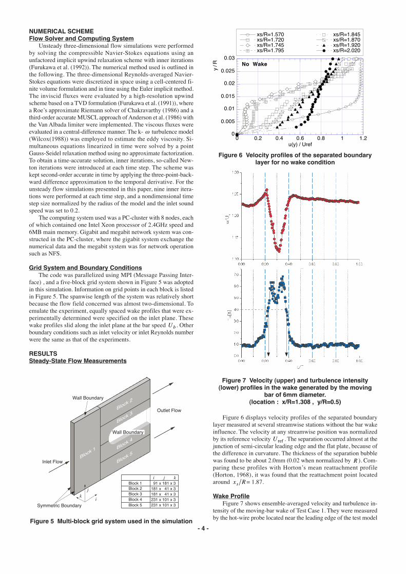
0.03No Wake

xs/R=1.570xs/R=1.720xs/R=1.745xs/R=1.795

xs/R=1.845xs/R=1.870xs/R=1.920xs/R=2.020

u(y) / Uref

y / R

NUMERICAL SCHEMEFlow Solver and Computing System

Unsteady three-dimensional flow simulations were performedby solving the compressible Navier-Stokes equations using anunfactored implicit upwind relaxation scheme with inner iterations(Furukawa et al. (1992)). The numerical method used is outlined inthe following. The three-dimensional Reynolds-averaged Navier-Stokes equations were discretized in space using a cell-centered fi-nite volume formulation and in time using the Euler implicit method.The inviscid fluxes were evaluated by a high-resolution upwindscheme based on a TVD formulation (Furukawa et al. (1991)), wherea Roe’s approximate Riemann solver of Chakravarthy (1986) and athird-order accurate MUSCL approach of Anderson et al. (1986) withthe Van Albada limiter were implemented. The viscous fluxes wereevaluated in a central-difference manner. The k- ω turbulence model(Wilcox(1988)) was employed to estimate the eddy viscosity. Si-multaneous equations linearized in time were solved by a pointGauss-Seidel relaxation method using no approximate factorization.To obtain a time-accurate solution, inner iterations, so-called New-ton iterations were introduced at each time step. The scheme waskept second-order accurate in time by applying the three-point-back-ward difference approximation to the temporal derivative. For theunsteady flow simulations presented in this paper, nine inner itera-tions were performed at each time step, and a nondimensional timestep size normalized by the radius of the model and the inlet soundspeed was set to 0.2.

The computing system used was a PC-cluster with 8 nodes, eachof which contained one Intel Xeon processor of 2.4GHz speed and6MB main memory. Gigabit and megabit network system was con-structed in the PC-cluster, where the gigabit system exchange thenumerical data and the megabit system was for network operationsuch as NFS.

Grid System and Boundary ConditionsThe code was parallelized using MPI (Message Passing Inter-

face) , and a five-block grid system shown in Figure 5 was adoptedin this simulation. Information on grid points in each block is listedin Figure 5. The spanwise length of the system was relatively shortbecause the flow field concerned was almost two-dimensional. Toemulate the experiment, equally spaced wake profiles that were ex-perimentally determined were specified on the inlet plane. Thesewake profiles slid along the inlet plane at the bar speed U b . Otherboundary conditions such as inlet velocity or inlet Reynolds numberwere the same as that of the experiments.

RESULTSSteady-State Flow Measurements

Figure 7 Velocity (upper) and turbulence intensity(lower) profiles in the wake generated by the moving

bar of 6mm diameter.(location : x/R=1.308 , y/R=0.5)

Figure 6 displays velocity profiles of the separated boundarylayer measured at several streamwise stations without the bar wakeinfluence. The velocity at any streamwise position was normalizedby its reference velocity U ref . The separation occurred almost at thejunction of semi-circular leading edge and the flat plate, because ofthe difference in curvature. The thickness of the separation bubblewas found to be about 2.0mm (0.02 when normalized by R ). Com-paring these profiles with Horton’s mean reattachment profile(Horton, 1968), it was found that the reattachment point locatedaround x Rs = 1.87.

Wake ProfileFigure 7 shows ensemble-averaged velocity and turbulence in-

tensity of the moving-bar wake of Test Case 1. They were measuredby the hot-wire probe located near the leading edge of the test model

Figure 6 Velocity profiles of the separated boundarylayer for no wake condition

Symmetric Boundary

Inlet Flow

Wall Boundary

Outlet Flow

Wall Boundary

Block 1

Block 2

Block 3

Block 4

Block 5

Block 1 91 x 181 x 3181 x 41 x 3181 x 41 x 3231 x 101 x 3231 x 101 x 3

Block 2Block 3Block 4Block 5

i

j k

i j k

Figure 5 Multi-block grid system used in the simulation

- 5 -

1.40

1.6

1.8

2.0

2.2

0.25 0.50 0.75 1.0 t / T

xs / R

90%%

%

100%U 1.40

1.6

1.8

2.0

2.2

0.25 0.50 0.75 1.0 t / T

xs / R

90%%

%

100%U

( x Rs = 1.308 and y R = 0.5) during one wake passing period.The data shown here was normalized by the inlet velocity U in . De-spite a flow acceleration near the leading edge, the velocity deficitof the wake retained about 0.2U in and the maximum wake turbu-lence was about 7%. Note that two peaks in the turbulence intensitydue to the shear layer of the wake were clearly observed. It followsfrom this figure that the wake with more than 4% turbulence inten-sity, which can be regarded as an effective turbulence intensity ac-cording to the suggestion of Funazaki et al. (1997), lasted for about15% of the bar passing period.

Emergence of Turbulence Spots and Calmed RegionDiscussion using boundary layer parameters Figure 8 shows con-tours of the ensemble-averaged displacement and momentum thick-nesses on the xs -time plane for Test Case 1 (the bar moving up-wards). Also shown in this figure are five lines on each of the con-tours, which represent traces of the fluid particles moving at 100%,90%, 50% and 30% speed of U ref , streamwisely averaged velocityof U ref over the measurement region. In Figure 8, the wide zone of

large displacement thickness appeared from x Rs = 1.6 to x Rs =1.8, which was caused by the separation bubble.

Before going into detail of the wake interaction with the separa-tion bubble, a brief comment seems necessary on how the positionsof those lines were determined. Because of its low velocity and con-sequently large value of ymax , the incoming wake tended to leaveits footprint in terms of a strip of relatively large displacement thick-ness. Taking advantage of this tendency, the wake path on the con-tour of the displacement thickness was easily spotted as shown inthe left contours of Figure 8. The positions of the 100% speed traceswere accordingly determined so that they fitted the strip of largedisplacement thickness. There appeared a triangle zone of large valueon the displacement thickness contours. Since this zone could beregarded as a consequence of wake-induced turbulence spots grow-ing towards the downstream, particle traces of 90% and 50% speedwere chosen to sketch out the zone, where the starting points of eachof the traces were placed on the same position. A trace of 30 %speed, which may represent the rear end of calmed region [1], alsostarted from the same point as the 90% and 50% traces. The sametraces were used in the momentum thickness contours without anymodifications. It turned out that the procedure to determine the po-sitions of the traces worked quite well in Test Case 1, and as will beshown in the following, the same approach was actually found to bevalid in other test cases, except for Test Case 2.

From the above discussions, it can be concluded that the tri-angle-shaped zone of large displacement thickness identified afterthe wake passage was the consequence of wake-induced turbulencespots. Besides, the momentum thickness data elucidated an areamarked by the circle. This area, which had relatively larger momen-tum thickness inside, almost laid itself underneath the path enclosedby 90% and 50% speed traces. Since increase in momentum thick-ness usually means the progress of boundary layer transition, theappearance of this area also supports the conclusion here that theincoming wake induced turbulent spots that strongly affected theseparation bubble. The important point here is that the spots in thiscase abruptly emerged almost at or rather upstream of the separationpoint. This was probably because of the adverse pressure gradientobserved by Funazaki et al. (2000) or the change in curvature as acatalyst of the transition, although much remains to be studied in thefuture. As discussed in the following, onset points of the turbulentspots, which were determined by the curve-fitting approach, exhib-ited a slight dependency to the flow conditions such as Reynoldsnumber or Strouhal number.

Figure 8 Ensemble-averaged displacement and mo-mentum thicknesses on xs - time planes for Test case 1(left : Displacement thickess / right : Momentum Thick-

ness)

0.00 0.50 1.00 1.50 2.00 x 10-2δ1 / R

0.10 0.40 0.70 1.00 1.30 x 10-2

δ2 / R

Figure 9 Composite 3D representation showing velocityfluctuation, turbulence intensity and velocity profile for

Test case 1

time

xs

Decelerated Zone (Wake)

Decelerated Zone (Turbulent Spot)

Decelerated Zone (Separation Bubble)

High Turbulence Intensity Zone

Velocity Contours

y

u / Uref0.00 0.25 0.50 0.75 1.00 1.25

Figure 10 Ensemble-averaged velocity on xs - timeplanes for Test case 1

(left : y/R = 0.005 / right : y/R = 0.020)

y/R=0.0051.40

1.6

1.8

2.0

2.2

0.25 0.50 0.75 1.0 t / T

xs / R

90%%

%

100%Uap

y/R=0.0201.40

1.6

1.8

2.0

2.2

0.25 0.50 0.75 1.0 t / T

xs / R

90%%

%

100%Uap

u / Uref0.00 0.25 0.50 0.75 1.00 1.25

- 6 -

Discussion using velocity fluctuation and turbulence intensity Fig-ure 9 shows a composite representation of velocity fluctuation, tur-bulence intensity and velocity profile in xs , y and time domain forTest Case 1. This figure clearly demonstrates the existence of theincoming wake and the appearance of the induced turbulence spotsbehind the wake in terms of the decelerated zone, where the decel-eration was measured from the local averaged velocity (see Eq. (2)).High turbulence intensity zone, which contained more than 14% lo-cal turbulence intensity and was pink-colored in this figure, startedto shrink after the passage of those decelerated zone. Since the highturbulence intensity originated mostly from unstable shear layer ofthe separation bubble, this shrinkage indicated that the wake pas-sage surely suppressed the separation bubble for relatively long pe-riod.

Effects of the Bar-Moving Direction and Strouhal NumberTest Case 1 (bar moving upwards) In Test Case 1, baseline case, thewide zone having large displacement thickness almost disappearedwhile the incoming wake swept over the test model, then recoveredafterwards. This indicates that the leading separation bubble experi-enced temporal suppression because of the passage of the incomingwake. Important features to be mentioned were found in Figure 8.The observation shows that the separation bubble with large dis-placement thickness remained almost unaffected even just beneaththe wake path. It seems that the wake passage itself did not make anexplicit contribution to the suppression of the separation bubble inthis case. In contrast, the reduction of the displacement thicknessindicates that the wake-induced turbulence spots and the followingcalmed region surely suppressed the separation bubble. A similarconclusion can be drawn from the observations of the ensemble-averaged velocity in Figure 10, where the low speed zone associ-ated with the separation bubble became small when the turbulentspots, then the calmed region passed over the separation bubble.

The turbulent spots, whose origin was identifiable from the in-tersection of the traces, slightly lagged behind the wake passage inthis case. The footprints of the wake passage could be recognized onthe near-wall plane ( y R = 0.005) as well as on the plane with itsheight from the wall almost same as that of the separation bubble( y R = 0.020) . On the plane of y R = 0.005 in Figure 10, the 100%speed traces could be shifted in the right direction from the originalposition of Figure 8 by some distance so that the traces agreed withthe wake passage footprint at the location denoted by the circle A.Since this shifting resulted in the attachment of the 100% traces to

the other traces, it can be stated that the turbulence spots actuallyemerged just after the wake passage near the surface. In other words,the upstream wake was mainly responsible for the generation of theturbulent spots. The shifted distance of the traces corresponded toabout 7% of the wake passing period, meaning that the wake suf-fered from large deformation due to the blockage effect of the testmodel and/or lagged behind the free-stream within the boundarylayer.

Circle B in Figure 10 shows that the separation bubble did notfully recover from the wake of the upstream wake passing even afterthe passage of the turbulent spots and the calmed region. One pos-sible reasoning on this phenomenon is “negative-jet effect” of theupstream wake interacting with the leading edge of the test model.

Figure 11 shows a snapshot of the numerical simulations show-ing the sequential interaction of the wake with separation bubbleson the both sides of the test model. The predicted separation bubbleexhibited considerable unsteady feature such as vortex shedding ina periodic manner. Although the code lacked ability to predict thetransitional behavior of the shear layer of the separation bubble, thesize of the bubble seemed to be reasonably predicted. The shed vor-tices moving downstream were considerably large in comparisonwith the size of the test model, which could not be verified throughthe present experiment because the shedding of the vortices was notnecessarily synchronized with the bar passing and the ensemble-averaging could not properly capture such non-synchronized flow

Figure 11 Computed result of wake-leading edgeinteraction

1.40

1.6

1.8

2.0

2.2

0.25 0.50 0.75 1.0 t / T

xs / R

100%U

%

%

%

1.40

1.6

1.8

2.0

2.2

0.25 0.50 0.75 1.0 t / T

xs / R

100%Uap

%%

Figure 12 Ensemble-averaged displacement and momen-tum thicknesses on xs - time planes for Test case 2

(left : Displacement thickess / right : Momentum Thick-ness)

0.250.00 0.50 0.75

0.02

0.04

0.06

0.08

y / R

t / T1.00 0.250.00 0.50 0.75

0.02

0.04

0.06

0.08

y / R

t / T

wake wake

turbulence spot

Test Case 1 Test Case 2

1.00

Figure 13 Bar wakes interacting with the separationbubble on y - time planes of ensemble-averaged veloc-

ity measured at xs / R = 1.745(left : Test Case 1 / right : Test Case 2)

0.00 0.50 1.00 1.50 2.00 x 10-2δ1 / R

0.10 0.40 0.70 1.00 1.30 x 10-2

δ2 / R

u / Uref0.00 0.25 0.50 0.75 1.00 1.25

Wake

- 7 -

event. Figure 11 indicates that the wake deformed around the leading

edge, interacting with the separation bubble. At a first glance, it doesnot seem that the wake passage had a drastic impact on the separa-tion bubble, which matches the experimental observation shown inFigure 9. However, the code was not able to predict the emergenceof turbulence spot. This means many subjects are left to be tackledin order to improve the ability of the code.

Test Case 2 (bar moving downwards) Figure 12 depicts contours ofthe ensemble-averaged displacement and momentum thicknesses onthe xs -time plane for Test Case 2 (the bar moving downwards) .Clearly, the wake duration in Test Case 2 was much longer than thatof Test Case 1. The separation bubble was gradually shrunk but notfully extinguished while the wake passed over it, which was in con-trast to Test Case 1. Rather surprisingly, wake-induced turbulencespots and calmed region were not clearly seen in this figure, althoughthe separation bubble was still suppressed even after the wake pas-sage. The appearance of the larger wake duration in the normal mov-ing case was already reported by Funazaki et al. (1997), which wasalso due to “negative-jet effect” . Figure 13 shows the ensemble-averaged velocities on the y-time planes for Test Case 1 (left) andTest Case 2 (right), again emphasizing the difference between thetwo cases in terms of bar-wake interaction with the separation bubble.The data in this figure was acquired at x Rs = 1.745 where theseparation bubble reached its maximum height in no wake case asshown in Figure 5. The left contours in Figure 13 clearly depict thatturbulent spots appeared behind the wake, penetrating the free-stream.Underneath the turbulent spots, the separation bubble, which wasexpressed by very low speed zone, was temporarily diminished. Onthe contrary, the wake in Test Case 2 was rather vague and did notseem to be accompanied by any turbulence spots. Furthermore, theseparation bubble in this case was not completely extinguished, whileit experienced the wake passage and its influence for longer timethan in Test Case 1. At this moment the reason for this distinct dif-ference has not been clarified yet.

Test Case 3 (higher Strouhal number) Figure 14 is the results ofTest Case 3; higher Strouhal number case. Since the Strouhal num-ber increased only by 25% of the original value, overall views of thedisplacement and momentum thickness contours quite resembled

those of Test Case 1. However, the onset of the wake-induced turbu-lence spots, which could be regarded as virtual origin of the spots,took place a little earlier than in Test Case 1, probably because ofenhanced wake turbulence.

Effects of the Mean Flow ConditionsFigure 15 shows two contours of the wake-affected displace-

ment thickness on xs -time diagrams obtained for Test Case 4 andTest Case 5. Since the Reynolds number was reduced by 25% inTest Case 4 or the incidence was increased from 0 deg to 5 deg, theseparation bubble for each of the test cases was larger than Test case1, which could be confirmed by looking at the extent of the highdisplacement thickness zone as well as at the peak value within thezone. Wake-induced turbulence spots clearly appeared, slowly be-ing lagged from the wake in both test cases. The onset of the turbu-lent spots in Test Case 4 (left of Figure 15) was found around x Rs= 1.6, while x Rs = 1.5 for Test case 1. This delay could be attrib-uted to the effect of the reduced Reynolds number. On the otherhand, the onset of the wake-induced turbulence spots in Test case 5started earlier than in Test case 1. This was probably because in ef-fect the surface length from the aerodynamic stagnation point to apoint concerned was elongated by about 0.09 in x Rs . Figure 16,ensemble-averaged velocity measured at x Rs = 1.745, indicates

Figure 14 Ensemble-averaged displacement andmomentum thicknesses on xs - time planes for Test

case 3(left : Displacement thickess / right : Momentum

Thickness)

1.4

1.6

1.8

2.0

2.2

0.25 0.50 0.75 1.0t / T

xs / R

100%Uap

%

%

%

1.4

1.6

1.8

2.0

2.2

0.25 0.50 0.75 1.0t / T

xs / R

100%Uap

%

%

%

1.4

1.6

1.8

2.0

2.2

0.25 0.50 0.75 1.0t / T

xs / R

100%Uap

%

%

%

1.4

1.6

1.8

2.0

2.2

0.25 0.50 0.75 1.0t / T

xs / R

100%Uap

%

%

%

Figure 15 Ensemble-averaged displacement andmomentum thicknesses on xs - time planes for Test

case 3(left : Test Case 4 / right : Test Case 5)

0.250.00 0.50 0.75

0.02

0.04

0.06

0.08

y / R

t / T1.00

Test Case 5

turbulence spot

wake

Figure 16 Bar wakes interacting with the separationbubble on y - time planes of ensemble-averaged veloc-

ity measured at xs / R = 1.745 (Test Case 5)

0.00 0.50 1.00 1.50 2.00 x 10-2δ1 / R

0.10 0.40 0.70 1.00 1.30 x 10-2

δ2 / R

u / Uref0.00 0.25 0.50 0.75 1.00 1.25

0.00 0.50 1.00 1.50 2.00 x 10-2δ1 / R

- 8 -

that wake-induced turbulent spots appeared behind the wake, abruptlydiminishing the separation bubble of very low speed zone. Thereaf-ter, the separation bubble started to recover in a gradual manner.

CONCLUSIONSThis study dealt with hot-wire probe measurements of separated

boundary layer around the leading edge of the blunt test model whichwas subjected to periodic wake passing. The focus of this study wason the effects of the direction of the wake-generating bar move-ment, wake-passing Strouhal number and the mean flow conditionssuch as Reynolds number. The findings in this study can be summa-rized as follows.(1) When the wake-generating bar moved upwards, the emergence

of wake-induced turbulence spot, followed by the resultantcalmed region, were identified behind the downstream wake inthe contours of the time-resolved displacement and momentumthicknesses on the distance-time planes or the ensemble-averagedvelocity.

(2) The turbulent spots emerged almost at or rather upstream of theseparation point. This rather early emergence of the turbulentspots could be reasoned by the effect of adverse pressure gradientor the change in curvature as a catalyst of the transition, althoughmuch remains to be studied in more detail. The onset of theturbulent spots onset slightly depended on the flow conditionssuch as Reynolds number or Strouhal number.

(3) The wake generated from the bar moving upwards did not makean explicit contribution to the suppression of the separationbubble. This was confirmed by the numerical simulation. Onthe contrary, the wake-induced turbulence spots and the followingcalmed region suppressed the separation bubble. The wake-affected separation bubble did not show quick recovery to thestate of no wake condition after the wake passage. One possibleexplanation on this phenomenon was “negative-jet effect” of theupstream wake interacting with the leading edge of the model.

(4) Wake-induced turbulence spots and calmed region were notclearly observed in the case when the wake-generating bar moveddownwards.

ACKNOWLEDGMENTSThe part of this work was conducted under the financial support

from the Ministry of Education and Science as Grants-in-Aid forScientific Research. The authors are indebted to invaluable supportsfrom Mr. F. Saito of Iwate University.

REFERENCESAnderson, W. K., Thomas, J. L., and van Leer, B., 1986, “Com-

parison of Finite Volume Flux Vector Splittings for the Euler Equa-tions, AIAA Journal, Vol. 24, No.9, pp. 1453-1460.

Brear, M.J., Hodson, H.P. and Harvey, N.W., 2001, “PressureSurface Separations in Low Pressure Turbines: Part 1 of 2 - MidspanBehaviour,” ASME Paper 2001-GT-0437.

Chakravarthy, S. R., 1984, “Relaxation Method for UnfactoredImplicit Upwind Schemes,” AIAA Paper No. 84-0165.

Chun, S. and Sung, J., 2002, “Influence of Unsteady Wake on aTurbulent Separation Bubble,” Experiments in Fluids, Vol. 32,pp.269-279.

Cumptsy, N.A., Dong, Y., and Li, Y.S., 1995, “CompressorBlade Boundary Layers in the Presence of Wakes,” ASME Paper95-GT-443.

Halstead, D.E., Wisler, D.C., Okiishi, T.H., Walker, G.J.,Hodson, H.P. and Shin, H.-W., 1995a, “Boundary layer Develop-ment in Axial Compressors and Turbines, Part 1 of 4: CompositePicture,” ASME Trans., Journal of Turbomachinery, Vol. 119, pp.114-127.

Funazaki, K., Harada, Y , Takahashi, E., 2000, “Control of Sepa-ration Bubble on a Blade Leading Edge by a Stationary bar Wake,”ASME Paper 2000-GT-267.

Funazaki, K. and Kato, Y., 2002, “Studies on a Blade LeadingEdge Separation Bubble Affected by Periodic Wakes: Its Transitional

Behavior and Boundary Layer Loss Reduction,”, ASME Paper GT-2002-30221.

Funazaki, K., Kitazawa, T., Koizumi, K. and Tanuma, T., 1997,“Studies on Wake-Disturbed Boundary layers under the Influencesof Favorable Pressure Gradient and Free-Stream Turbulence-PartI:Experimental Setup and Discussions on Transition Model,” ASMEPaper 97-GT-52.

Furukawa, M., Nakano, T., and Inoue, M., 1992, “UnsteadyNavier-Stokes Simulation of Transonic Cascade Flow Using anUnfactored Implicit Upwind Relaxation Scheme With Inner Itera-tions”, ASME Trans., Journal of Turbomachinery, Vol. 114, No.3,pp. 599-606.

Furukawa, M., Yamasaki, M., and Inoue, M., 1991, “A ZonalApproach for Navier-Stokes Computations of Compressible Cas-cade Flow Fields Using a TVD Finite Volume Method,” ASMETrans., Journal of Turbomachinery, Vol. 113, No.4, pp. 573-582.

Halstead, D.E., Wisler, D.C., Okiishi, T.H., Walker, G.J.,Hodson, H.P. and Shin, H.-W., 1995b, “Boundary layer Develop-ment in Axial Compressors and Turbines, Part 2 of 4: Compres-sors,” ASME Trans., Journal of Turbomachinery, Vol. 119, pp. 426-444.

Halstead, D.E., Wisler, D.C., Okiishi, T.H., Walker, G.J.,Hodson, H.P. and Shin, H.-W., 1995c, “Boundary layer Develop-ment in Axial Compressors and Turbines, Part 3 of 4: Low PressureTurbines,” ASME Trans., Journal of Turbomachinery, Vol. 119, pp.225-237.

Halstead, D.E., Wisler, D.C., Okiishi, T.H., Walker, G.J.,Hodson, H.P. and Shin, H.-W., 1995d, “Boundary layer Develop-ment in Axial Compressors and Turbines, Part 4 of 4: Computationsand Analyses,” ASME Trans., Journal of Turbomachinery, Vol. 119,pp. 225-237.

Horton, H.P., 1968, “ A Semi-Empirical Theory for the Growthand Bursting of Laminar Separation Bubbles,” Aeronautical ResearchCouncil, CP-1073.

Kaszeta, R.W., Simon, T.W. and Ashpis, D.E., 2001, “Experi-mental Investigation of Transition to Turbulence as Affected by Pass-ing Wakes,” ASME Paper 2001-GT-0195.

Ottavy, X., Vilmin, S., Opoka, M., Hodson, H. and Gallimore,S., 2002, “The Effects of Wake-Passing Unsteadiness over a HighlyLoaded Compressor-Like Flat Plate,” ASME Paper GT-2002-30354.

Paxson, D.E. and Mayle, R.E., 1990, “Laminar Boundary LayerInteraction with an Unsteady Passing Wake,” ASME Paper 90-GT-120.

Schulte, V. and Hodson, H.P., 1994, “Wake-Separation BubbleInteraction in Low Pressure Turbines,” AIAA Paper AIAA-94-2931.

Van Treuren, K. W., Simon, T., von Koller, M., Byerley, A.R.,Baughn, J.W. and Rivir, R., 2002, “Measurements in a Turbine Cas-cade Flow under Ultra Low Reynolds Number Conditions,” ASMETrans., J. Turbomachinery, 124, pp. 100-106.

Wilcox, D. C., 1988, “Reassessment of the Scale-DeterminingEquation of Advanced Turbulence Models,” AIAA Journal, Vol. 26,No. 11, pp. 1299-1310.