novel signal processing strategies for better melody
TRANSCRIPT

SIGNAL PROCESSING STRATEGIES FOR BETTER MELODY RECOGNITION AND
IMPROVED SPEECH UNDERSTANDING IN NOISE
FOR COCHLEAR IMPLANTS
APPROVED BY SUPERVISORY COMMITTEE:
Dr. Philipos C. Loizou, Chair
Dr. John H. L. Hansen
Dr. John P. Fonseka
Dr. Mohammad Saquib

© Copyright 2006
Kalyan S. Kasturi
All Rights Reserved

To my dear parents, brother and sister

SIGNAL PROCESSING STRATEGIES FOR BETTER MELODY RECOGNITION AND
IMPROVED SPEECH UNDERSTANDING IN NOISE
FOR COCHLEAR IMPLANTS
by
KALYAN S. KASTURI, B.TECH., M.S.
DISSERTATION
Presented to the faculty of
The University of Texas at Dallas
in Partial Fulfillment
of the Requirements
for the Degree of
DOCTOR OF PHILOSOPHY IN ELECTRICAL ENGINEERING
THE UNIVERSITY OF TEXAS AT DALLAS
December 2006

v
ACKNOWLEDGEMENTS I would like to thank my advisor Dr. Philip Loizou, for giving me the opportunity to work in
various research projects related to the field of cochlear implants. I have immensely benefited
from his valuable advice and constant support through out my doctoral program.
Next, I want to express my respects to Dr. John Hansen obliging to be on my defense
committee and providing valuable suggestions.
I thank Dr. John Fonseka for being kind to agree to serve on the committee and giving useful
feedback on this manuscript.
I thank Dr. Mohammad Saquib for serving on the committee, giving helpful advice and
feedback on this manuscript.
I also thank Dr. Lorenzo Turicchia, Dr. Rahul Sarpeshkar, Dr. Michael Dorman, Dr. Anthony
Spahr, Dr. Arthur Lobo and Dr. Yi Hu for their help.
Finally, I express my gratitude to NIDCD/NIH (Grant No. R01 DC03421 and R01
DC007527) for their support.
November 2006

vi
SIGNAL PROCESSING STRATEGIES FOR BETTER MELODY RECOGNITION AND
IMPROVED SPEECH UNDERSTANDING IN NOISE
FOR COCHLEAR IMPLANTS
Publication No. ___________________
Kalyan S. Kasturi, Ph.D. The University of Texas at Dallas, 2006
Supervising Professor: Dr. Philipos C. Loizou Cochlear implants are prosthetic devices, consisting of implanted electrodes and a signal
processor and are designed to restore partial hearing to the profoundly deaf community.
Since their inception in early 1970s cochlear implants have gradually gained popularity and
consequently considerable research has been done to advance and improve the cochlear
implant technology. Most of the research conducted so far in the field of cochlear implants
has been primarily focused on improving speech perception in quiet. Music perception and
speech perception in noisy listening conditions with cochlear implants are still highly
challenging problems. Many research studies have reported low recognition scores in the task
of simple melody recognition. Most of the cochlear implant devices use envelope cues to
provide electric stimulation. Understanding the effect of various factors on melody
recognition in the context of cochlear implants is important to improve the existing coding
strategies. In the present work we investigate the effect of various factors such as filter

vii
spacing, relative phase, spectral up-shifting, carrier frequency and phase perturbation on
melody recognition in acoustic hearing. The filter spacing currently used in the cochlear
implants is larger than the musical semitone steps and hence not all musical notes can be
resolved. In the current work we investigate the use of new filter spacing techniques called
the ‘Semitone filter spacing techniques’ in which filter bandwidths are varied in
correspondence to the musical semitone steps. Noise reduction methods investigated so far
for use with cochlear implants are mostly pre-processing methods. In these methods, the
speech signal is first enhanced using the noise reduction method and the enhanced signal is
then processed using the speech processor. A better and more efficient approach is to
integrate the noise reduction mechanism into the cochlear implant signal processing. In this
dissertation we investigate the use of two such embedded noise reduction methods namely,
the ‘SNR weighting method’ and the ‘S-shaped compression’ to improve speech perception
in noisy listening conditions. The SNR weighting noise reduction method is an exponential
weighting method that uses the instantaneous signal to noise ratio (SNR) estimate to perform
noise reduction in each frequency band that corresponds to a particular electrode in the
cochlear implant. The S-shaped compression technique divides the compression curve into
two regions based on the noise estimate. This method applies a different type of compression
for the noise portion and the speech portion and hence better suppresses the noise compared
to the regular power-law compression.

viii
TABLE OF CONTENTS
ACKNOWLEDGEMENTS…………………………………………………………………...v ABSTRACT………………………………..………………………………………………...vi LIST OF FIGURES…………………………………………………………………………xiv LIST OF TABLES………………………………………………………………………….xvii CHAPTER 1 INTRODUCTION………………………………………….……...…….…..1
CHAPTER 2 INTRODUCTION TO COCHLEAR IMPLANTS………..……...…….…...6
2.1 Physiology of the human ear………………………………………………………..6
2.2 Normal hearing mechanism……………………………………………………..….9
2.3 Hearing loss and cochlear implants……………………………………………….11
2.4 Basic functional mechanism of a cochlear implant……………………………….12
2.5 Classification of cochlear implant devices………………………………………..14
2.6 Performance metrics for cochlear implant………………………………………...15
2.7 Early single-channel cochlear implant devices……………………………………15
2.8 Multi-channel cochlear implants…………………………………………………..16
2.9 Commercial multi-channel cochlear implant device manufacturers……………...16
ix
2.10 Signal processing strategies for multi-channel cochlear implants………………...17
2.11 Some representative feature extraction strategies…………………………………19 2.11.1 F0/F1/F2 Strategy……………………………………………………………19 2.11.2 MPEAK Strategy…………………………………………………………….21
2.12 Some representative waveform based strategies…………………………………..22 2.12.1 Compressed Analog (CA) Strategy………………………………………….22 2.12.2 Simultaneous Analog (SAS) Strategy………………………………………..22 2.12.3 Continuous Interleaved Sampling (CIS) Strategy……………………………23 2.12.4 SPEAK Strategy……………………………………………………………...25 2.12.5 ACE Strategy………………………………………………………………...26
2.13 Currently available commercial processors……………………………………….27 2.13.1 Clarion CII / Auria device……………………………………………………27 2.13.2 Nucleus-24 / Esprit 3G / Freedom device……………………………………28 2.13.3 Combi-40+ / PULSARci100 device…………………………………………..28
CHAPTER 3 LITERATURE REVIEW………………………………..........……………29
3.1 Chapter Outline……………………………………………………………………29
3.2 Music perception with cochlear implants…………………………………………30 3.2.1 Various parameters governing music perception……………………………….30 3.2.2 Perception of pitch versus rhythm in cochlear implants………………………..31 3.2.3 Recognition of simple melodies using electrical amplitude variations in cochlear implants…………………………………………………………………………………34

x
3.2.4 Simple melody recognition using pulse rate variations to convey pitch information……………………………………………………………………………...36
3.2.5 Recognition of real world musical pieces using the current cochlear implant devices …………………………………………………………………………………..37
3.3 Strategies to better code fundamental frequency (F0) information……………….39 3.3.1 Strategies for enhancing spectral cues………………………………………….39 3.3.2 Strategies for enhancing temporal cues………………………………………...41
3.4 Effect of background noise on speech perception with cochlear implants………..42 3.4.1 Effect of speech-shaped noise on consonant and sentence recognition using the CIS strategy……………………………………………………………………………..42
3.4.2 Effect of speech-shaped noise on consonant and vowel recognition using SPEAK strategy………………………………………………………………………...43
3.4.3 Effect of speech-shaped noise on consonant, vowel and sentence recognition using SPEAK, CIS and SAS strategies…………………………………………………44
3.4.4 Effect of multi-talker babble noise on sentence recognition using SPEAK, CIS and SAS strategy………………………………………………………………………..45
3.5 Review of various techniques used in the general area of speech enhancement….46 3.5.1 Spectral subtraction technique for speech enhancement……………………….47 3.5.2 Nonlinear Spectral subtraction technique for speech enhancement……………48 3.5.3 Use of Wiener filtering for performing speech enhancement…………………..49 3.5.4 MMSE estimation of spectral amplitude for speech enhancement……………..51
3.5.4.1 Decision directed estimation for computation of a priori SNR…………...52
3.5.5 Maximum likelihood envelope estimation for speech enhancement…………...53
3.6 Noise reduction techniques implemented for Cochlear implants…………………53 3.6.1 Use of adaptive beam forming for noise reduction in cochlear implants………54

xi
3.6.2 Use of nonlinear spectral subtraction for noise reduction in cochlear implants..55 3.6.3 Use of signal subspace technique for noise reduction in cochlear implants……58
3.7 Use of amplitude compression in cochlear implants……………………………...60 3.7.1 Effect of power law compression on phoneme recognition in cochlear implants…………………………………………………………………………………60 3.7.2 Effect of power exponent variations on consonant recognition in cochlear implants…………………………………………………………………………………62 3.7.3 Effect of compression on speech perception in noise with cochlear implants…63
CHAPTER 4 STRATEGIES FOR IMPROVING MELODY RECOGNITION WITH COCHLEARIMPLANTS…………..…………………………………………………….….65
4.1 Motivation…………………………………………………………………………65
4.2 Investigation of various factors affecting music perception………………………67 4.2.1 Effect of filter spacing on melody recognition in acoustic hearing…………….68
4.2.1.1 Experimental Method……………………………………………………..68 4.2.1.2 Results and Discussion……………………………………………………78
4.2.2 Effect of Spectral shift on melody recognition in acoustic hearing…………….82
4.2.2.1 Experimental Method……………………………………………………..82
4.2.2.2 Results and discussion…………………………………………………….85
4.2.3 Effect of relative phase on melody recognition in acoustic hearing……………87
4.2.3.1 Experimental Method……………………………………………………..87 4.2.3.2 Results and Discussion……………………………………………………91
4.2.4 Effect of carrier frequency for synthesis on melody recognition in acoustic hearing…………………………………………………………………………………..96

xii
4.2.4.1 Experimental Method……………………………………………………...97 4.2.4.2 Results and Discussion…………………………………………………....98
4.2.5 Effect of perturbation in phase information on melody recognition in acoustic hearing…………………………………………………………………………………100
4.2.5.1 Experimental Method…………………………………………………….101 4.2.5.2 Results and Discussion…………………………………………………..102
4.3 Novel filter spacing techniques for better music perception in electric hearing…103 4.3.1 Experimental Method…………………………………………………………103 4.3.2 Results and Discussion………………………………………………………..117
CHAPTER 5 STRATEGIES FOR BETTER SPEECH PERCEPTION IN NOISE WITH COCHLEAR IMPLANTS………………………………………………………………….124
5.1 Motivation………………………………………………………………………..124
5.2 SNR weighting noise reduction method…………………………………………126 5.2.1 Experimental Method………………………………………………………….126 5.2.2 Results and discussion………………………………………………………...132
5.3 Effect of SNR estimation in individual channels on SNR weighting method…...135
5.3.1 Experimental Method………………………………………………………….136 5.3.2 Results and Discussion………………………………………………………..138
5.4 Novel S-shaped compression techniques for noise suppression…………………141 5.4.1 Theoretical derivation of various S-shaped compression curves……………...141
5.4.1.1 S-shaped compression……………………………………………………142
5.4.2 Evaluation of S-shaped compression techniques for noise reduction in cochlear implants………………………………………………………………………………..146

xiii
5.4.2.1 Experimental Method…………………………………………………….146 5.4.2.2 Results and Discussion…………………………………………………..155
CHAPTER 6 CONCLUSIONS……………………………………………..…………...162
6.1 Major Contributions of this dissertation…………………………………………164
6.2 Future Work……………………………………………………………………...165
REFERENCES……………………………………………………………………………..166 VITA
xiv
LIST OF FIGURES Figure 2.1. A block diagram representation of the human hearing system…………………...7 Figure 2.2. A diagrammatic representation depicting various important parts of the human cochlea………………………………………………………………………………………...8 Figure 2.3. A diagram representing the hair cell transduction mechanism………………….10 Figure 2.4. Normal hearing systems versus impaired hearing system……………………….11 Figure 2.5. A bock diagram representation of the cochlear implant…………………………13 Figure 2.6. A block diagram representation of the Continuous Interleaved Sampling (CIS) strategy……………………………………………………………………………………….24 Figure 4.1. The filter spacing using 12 channels of semitone spacing………………………72 Figure 4.2. The filter spacing using 12 channels of log spacing with large bandwidth……...73 Figure 4.3. The filter spacing using 12 channels of log spacing with small bandwidth……..74 Figure 4.4. A block diagram representation of noise band simulation………………………77 Figure 4.5. Effect of filter spacing: Semitone Spacing versus Log Spacing on melody recognition as a function of number of spectral channels……………………………………78 Figure 4.6. Effect of Signal Bandwidth: Log Spacing with Large Bandwidth versus Log Spacing with Small Bandwidth on melody recognition as a function of number of spectral channels………………………………………………………………………………………80 Figure 4.7. Effect of upward spectral shift on melody recognition using semitone filter spacing with four channels…………………………………………………………………...86 Figure 4.8. A block diagram representation of sinusoidal synthesis incorporating phase information…………………………………………………………………………………...89 Figure 4.9. Effect of relative phase on melody recognition for music informed subjects…...91 Figure 4.10. Effect of relative phase on melody recognition for music naïve subjects……...92

xv
Figure 4.11. Effect of carrier frequency for synthesis on melody recognition for single-channel case………………………………………………………………………………...98 Figure 4.12. Effect of carrier frequency for synthesis on melody recognition for two-channel case………………………………………………………………………………………….99 Figure 4.13. Effect of phase perturbation on melody recognition………………………….102 Figure 4.14. The filter spacing using 16 channels of log spacing (16LOG)………………..107 Figure 4.15. The filter spacing using 6 channels of semitone spacing (6SM)……………...108 Figure 4.16. The filter spacing using 16 channels of 6SM+LOG hybrid spacing………….115 Figure 4.17. Mean percent correct scores for melody recognition………………………...117 Figure 4.18. Individual subject scores for comparison of 16LOG and 4SM strategies…….118 Figure 4.19. Individual subject scores for comparison of 16LOG and 4SM+LOG strategies……………………………………………………………………………………118 Figure 4.20. Individual subject scores for comparison of 16LOG and 6SM strategies…….119 Figure 4.21. Individual subject scores for comparison of 16LOG and 6SM+LOG strategies……………………………………………………………………………………119 Figure 4.22. Individual subject scores for comparison of 16LOG and 12SM strategies…...120 Figure 4.23. Individual subject scores for comparison of 16LOG and 12SM+LOG strategies……………………………………………………………………………………120 Figure 5.1. Block diagram representation for SNR weighting method…………………….127 Figure 5.2. A plot of the exponential weighting function depicting the gain as a function of SNR. The Wiener gain function is also shown for comparison…………………………….130 Figure 5.3. Mean vowel recognition in presence of speech-shaped noise using SNR weighting method…………………………………………………………………………...133 Figure 5.4. Individual subject scores for vowel recognition in presence of speech-shaped noise using SNR weighting method………………………………………………………...133 Figure 5.5. Mean sentence recognition in presence of speech-shaped noise using SNR weighting method…………………………………………………………………………...134

xvi
Figure 5.6. Individual subject scores for sentence recognition in presence of speech-shaped noise using SNR weighting method………………………………………………………...135 Figure 5.7. Effect of SNR estimation in individual channels for the case of multi-talker babble noise at 10 dB SNR…………………………………………………………………139 Figure 5.8. Regular power-law compression using an exponent p=-0.0001……………….142 Figure 5.9. S-shaped compression (Type 1) using power exponents p1=-0.0001, p2=1.8….143 Figure 5.10. S-shaped compression (Type 1) using power exponents p1=-0.0001, p2=1.8 (zoomed in around the knee point)…………………………………………………………144 Figure 5.11. S-shaped compression (Type 2) using power exponents p1=-0.0001, p2=1…..145 Figure 5.12. S-shaped compression (Type 2) using power exponents p1=-0.0001, p2=1(zoomed in around the knee point)…………………………………………………….146 Figure 5.13. Envelope of noise and the noise envelope estimated using the algorithm……151 Figure 5.14. Speech envelopes estimated with and without using S-shaped compression…153 Figure 5.15. Mean sentence recognition scores in presence of speech-shaped noise at 5 dB SNR using S-shaped compression………………………………………………………….155 Figure 5.16. Individual subject scores for sentence recognition in presence of speech-shaped noise at 5 dB SNR using S-shaped compression…………………………………………...156 Figure 5.17. Mean sentence recognition scores in presence of multi-talker babble noise at 10 dB SNR using S-shaped compression………………………………………………………157 Figure 5.18. Individual subject scores for sentence recognition in presence of multi-talker babble noise at 10 dB SNR using S-shaped compression…………………………………..157 Figure 5.19. Mean sentence recognition scores in presence of multi-talker babble noise at 5 dB SNR using S-shaped compression………………………………………………………158 Figure 5.20. Individual subject scores for sentence recognition in presence of multi-talker babble noise at 5 dB SNR using S-shaped compression……………………………………159

xvii
LIST OF TABLES
Table 4.1. The 3-dB frequency boundaries of the 2 bands using semitone spacing with the corresponding center frequencies (Hz) of each band.............................................................. 70 Table 4.2. The 3-dB frequency boundaries of the 4 bands using semitone spacing with the corresponding center frequencies (Hz) of each band.............................................................. 70 Table 4.3. The 3-dB frequency boundaries of the 6 bands using semitone spacing with the corresponding center frequencies (Hz) of each band.............................................................. 71 Table 4.4. The 3-dB frequency boundaries of the 12 bands using semitone spacing with the corresponding center frequencies (Hz) of each band.............................................................. 71 Table 4.5. The 3-dB frequency boundaries of the 12 bands using large bandwidth logarithmic spacing with the corresponding center frequencies (Hz) of each band. .............. 74 Table 4.6. The 3-dB frequency boundaries of the 12 bands using small bandwidth logarithmic spacing with the corresponding center frequencies (Hz) of each band. .............. 75 Table 4.7. The 3-dB frequency boundaries of the 4 bands using logarithmic spacing (Log2) with the corresponding center frequencies (Hz) of each band................................................ 84 Table 4.8. The 3-dB frequency boundaries of the 4 bands with spectral up-shifting using logarithmic spacing (Log2 - shifted) with the corresponding center frequencies (Hz). ......... 84 Table 4.9. The 3-dB frequency boundaries of the 4 bands with spectral up-shifting using semitone spacing (semitone - shifted) with the corresponding center frequencies (Hz) of each band......................................................................................................................................... 85 Table 4.10. The biographical data for the six cochlear implant subjects............................. 105 Table 4.11. The 3-dB frequency boundaries of the 16 bands for 16LOG strategy with the corresponding center frequencies (Hz) of each band............................................................ 106 Table 4.12. The 3-dB frequency boundaries of the 4 bands for 4SM strategy with the corresponding center frequencies (Hz) of each band............................................................ 109 Table 4.13. The 3-dB frequency boundaries of the 6 bands for 6SM strategy with the corresponding center frequencies (Hz) of each band............................................................ 109

xviii
Table 4.14. The 3-dB frequency boundaries of the 12 bands for 12SM strategy with the corresponding center frequencies (Hz) of each band............................................................ 110 Table 4.15. The 3-dB frequency boundaries of the 16 bands for 4SM+LOG strategy with the corresponding center frequencies (Hz) of each band............................................................ 112 Table 4.16. The 3-dB frequency boundaries of the 16 bands for 6SM+LOG strategy with the corresponding center frequencies (Hz) of each band............................................................ 113 Table 4.17. The 3-dB frequency boundaries of the 16 bands for 12SM+LOG strategy with the corresponding center frequencies (Hz) of each band...................................................... 114 Table 4.18. The percent preference scores for semitone filter spacing strategies over conventional logarithmic spacing strategy............................................................................ 122 Table 4.19. The distance measures for semitone filter spacing strategies over conventional logarithmic spacing strategy. ................................................................................................ 123 Table 5.1. The biographical data for the eight cochlear implant users who were the subjects for the experiments with SNR weighting method................................................................. 128 Table 5.2. The biographical data for the five cochlear implant users who were the subjects for the experiments with SNR estimation in individual channels......................................... 137 Table 5.3. The biographical data for the eight cochlear implant users who participated in the experiments with S-shape compression. ............................................................................... 147

1
CHAPTER 1
INTRODUCTION Perception of sound especially in the form of speech and music is one of the everyday
activities in the life of human beings. Profound hearing loss can severely affect the life of
a human being. Cochlear implants are devices designed to restore partial hearing to
profoundly deaf people. Cochlear implants consist of an electrode array inserted into the
inner ear and a signal processor that generates electrical stimuli from input speech signal.
The early cochlear implant devices were single-electrode devices. Most of the current
cochlear implant devices are multi-electrode devices that deliver electric stimuli
pertaining to the various frequency bands to the various regions in the cochlea. Many of
the research studies conducted in the field of cochlear implants so far have primarily
focused on how to improve the perception of speech with cochlear implants. Several
speech coding strategies have been developed by many research studies that present the
various features in the speech signal, for example speech envelope, fundamental
frequency (F0), first formant (F1) and second formant (F2) information in different ways
to improve speech perception with cochlear implants. A detailed literature review of
many of the research studies and signal processing strategies is presented in chapter two.
Perception of music (including simple melody recognition) and perception of
speech in noisy listening conditions are still challenging problems in the field of cochlear
implants. Many research studies have investigated the perception of common melodies
(e.g. ‘Twinkle Twinkle Little Star’, ‘Frere Jacques’) with the current cochlear implant

2
devices. Most of the studies have reported relatively poor melody recognition with
cochlear implant devices. To improve melody recognition with cochlear implants, we
need to investigate the various factors that affect melody recognition so as to add further
improvements into the existing strategies. In this dissertation, melody recognition
experiments were performed using cochlear implant simulations with normal hearing
listeners to quantify the effect of various factors on melody recognition. Most of the
current devices use a broad logarithmic spacing to perform spectral analysis. While this is
sufficient for speech perception, the same may not be true for melody recognition. Most
of the musical note’s bandwidth is relatively small compared to the logarithmic
bandwidths and hence the logarithmic spacing does not provide enough frequency
resolution to identify individual musical notes. In this dissertation we investigate the
effect of varying the filter spacing on melody recognition. We propose novel filter
spacing techniques, namely the ‘Semitone filter spacing techniques’ that use narrow
filters that correspond to musical semitone steps on the musical scale based on the
melodic center of gravity of the musical material.
Most of the cochlear implant processors mainly use envelope information and
discard phase information to deliver electrical pulses at a fixed rate to the various
electrodes. In the current work we investigate the effect of adding relative phase
information on melody recognition. We also investigate the effect of various other
factors namely spectral shifting, carrier frequency and phase perturbation on simple
melody recognition in the context of cochlear implants in acoustic hearing. As a logical
extension to these studies we conducted experiments with cochlear implant listeners to
assess the effect of the semitone filter spacing strategies on melody recognition.
3
Experiments on melody recognition and melodic preference were conducted to quantify
the performance of the semitone filter spacing techniques.
Researchers have investigated the use of noise reduction methods developed in
the general area of speech enhancement to improve speech perception in noise with
cochlear implants. Most of the noise reduction methods investigated so far use a pre-
processing approach to reduce the background noise. The corrupted speech signal is first
enhanced using a particular noise reduction method and the resulting enhanced speech is
then processed using the existing signal processing techniques to derive the electrical
stimulation for the cochlear implant. A more efficient method will be to embed the noise
reduction method into the existing cochlear signal processing strategies. In this
dissertation we investigate the use of two embedded noise reduction methods namely the
‘SNR weighting method’ and the ‘S-shaped compression’ to improve speech perception
in noise with cochlear implants. The SNR weighting noise reduction method uses an
exponential weighting similar to the generalized Wiener filter, in each frequency band to
perform noise reduction. Most of the cochlear implants use a compression function to
map the acoustic signals into the electric stimuli. Most of the devices use a power-law
function to perform the compression. In the case of speech corrupted by noise, the noise
signal portion and the speech signal portion are compressed in the same way. The
proposed S-shaped compression technique divides the compression curve into two
regions based on the computed noise estimate. The signal portion falling below the noise
estimate value is subjected to an expansive function and the signal portion falling above
the noise estimate value is subjected a compressive function to better suppress the noise
portion.

4
The major contributions of this dissertation are as follows:
Proposed a new filter spacing namely the ‘Semitone filter spacing’ that is based
on the musical semitone scale to improve melody recognition with the cochlear
implants.
Proposed the SNR weighting noise reduction method which is an exponential
weighting method that uses the instantaneous SNR estimate. This method is
embedded into the CIS strategy and has the advantages of low computational
complexity, ease of implementation and better control of noise reduction
mechanism.
Proposed new compression functions namely the S-shaped compression functions
that compress the speech and noise portions of the signal in different ways to
improve speech perception in noise. This is also a noise reduction method
embedded into the CIS strategy to effectively suppress the noise.
This dissertation is organized as follows:
In chapter two we introduce the cochlear implant devices and the research
developments made so far in the cochlear implant technology. In chapter three we review
the literature in the scientific community pertaining to melody recognition, speech
perception in noise and compression techniques used in the field of cochlear implants.
In chapter four we present the research work performed in this dissertation to
improve melody recognition. First we investigate the effect of various factors namely
filter spacing, spectral up-shifting, relative phase, carrier frequency and phase
perturbation on melody recognition in acoustic hearing. Next we investigate the effect of
the various semitone filter spacing techniques with cochlear implant users.

5
In chapter five we investigate the effect of the embedded noise reduction methods
for better speech perception in noise with cochlear implants. First we investigate the use
of the SNR weighting noise reduction method with cochlear implant users. Second we
investigate the effect of signal to noise ratio (SNR) estimation on the performance of the
noise reduction method. Finally, we present the use of the S-shaped compression
techniques to suppress noise, in order to improve speech understanding in noise with
cochlear implant recipients. In chapter six, we present the summary and conclusions from
this dissertation.

6
CHAPTER 2
INTRODUCTION TO COCHLEAR IMPLANTS Cochlear implants are prosthetic devices that restore partial hearing to the profoundly
deaf community. The ideology behind the use of cochlear implants is that partial hearing
can be restored by direct electrical stimulation of the auditory neurons. The study of
cochlear implants is a multi-disciplinary subject that covers many fields that include
signal processing, speech science, bioengineering, and physiology. One of the main
challenges in developing an efficient cochlear implant lies in deriving an optimal
electrical stimulus that can elicit neural sensations that correspond to those generated by
the normal hearing mechanism.
2.1 Physiology of the human ear
The human ear has exquisite intensity and frequency resolution capabilities. The dynamic
range of human hearing is about 120 dB, which corresponds to about 1210 intensity units
[1]. The frequency discrimination limens (DL) are about only 0.2% in the frequency
range from 1 to 2 kHz [33]. The human hearing system can be divided into four
functional units, (1) External ear, (2) Middle ear, (3) Inner ear and (4) Auditory nerve.
A diagrammatic representation of the human auditory system is shown in Figure
2.1. The first functional unit is the external ear which consists of the pinna and the
auditory canal. The second functional unit is the middle ear which consists of three small
bones called malleus, incus and stapes. The middle ear acts as acoustic impedance

7
matcher and increases the efficiency of transmission of sound by decreasing the amount
of sound reflection.
Figure 2.1. A block diagram representation of the human hearing system.
The third functional unit is the inner ear or the cochlea. The cochlea is filled with
fluids that are split in three chambers called scala vestibule, scala media and scala
External Ear
Middle Ear
Cochlea
Auditory Nerve
Incoming sound
Ensemble of neural signals
Peripheral Auditory System
Input to the System
Output of the System

8
tympani. The cochlea is a snail shaped structure with the beginning portion being called
the base and the ending portion being called the apex. A diagrammatic representation of
the human cochlea is shown in Figure 2.2.
Figure 2.2. A diagrammatic representation depicting various important parts of the human cochlea.
The cochlea is responsible to a large extent for the spectral analysis performed by
the human ear. From psychophysical experiments it is observed that the human auditory
system acts as a set of overlapping band-pass filters to perform spectral analysis. These
band-pass filters are termed as critical bands or auditory filters. The important part in the
Apex (Low frequency)
Oval window
Round window
Scala vestibule
Scala tympani
Basilar membrane (Roughly 34 mm in length)
Scala media
Base (High frequency)
Pressure gradient

9
cochlea is the basilar membrane which is situated between the scala media and the scala
tympani. The basilar membrane is roughly about 34 mm in length extending from base to
apex. The auditory filter bandwidth roughly corresponds to 0.9 mm of distance along the
basilar membrane. On top of the basilar membrane is situated the organ of corti which
carries the vital transduction hair cells. There are two types of hair cells namely outer hair
cells and inner hair cells.
2.2 Normal hearing mechanism
The sound travels through the auditory canal and impinges on the tympanic membrane
causing it to vibrate. The vibrations of the tympanic membrane are transmitted through
the bones in the middle ear to the inner ear, with the stapes causing pressure variations on
the oval window. These pressure variations cause the cochlear fluid to move to and fro in
synchrony with the sound. This pressure gradient forces the basilar membrane to vibrate
in synchrony with the sound.
The basilar membrane vibrates in a characteristic manner in response to a sound.
The traveling pressure wave reaches a peak at a particular point along the basilar
membrane, depending upon the frequency of the sound. High frequency sounds give rise
to a peak near the base and low frequency sounds give rise to a peak near the apex. Each
place along the basilar membrane responds best to one frequency although it responds to
other frequencies as well. This is called tonotopic organization of the basilar membrane.
This gives rise to the frequency/place theory which accounts for the spectral resolution
properties of the human ear.

10
The vibrations of the basilar membrane cause a shearing force on the hair cells
causing them to bend. The bending of the hair cells generates receptor potentials that
trigger the auditory nerve fibers. The transduction of the outer hair cells accounts for the
basilar membrane compression. The vibrations of the basilar membrane are selectively
amplified and compressed by the outer hair cells. The outer hair cells provide level
dependent and frequency dependent gain control and aid in the exquisite sensitivity and
frequency resolving capabilities of the ear. Finally the transduction of the inner hair cells
triggers the auditory nerve fibers that carry information to the brain. A pictorial depiction
of the hair cell transduction mechanism is given in Figure 2.3.
Figure 2.3. A diagram representing the hair cell transduction mechanism.
Basilar membrane
Basilar membrane vibrations
Auditory nerve
Hair cells
Bending of hair cells – Trigger to auditory nerve fibers

11
2.3 Hearing loss and cochlear implants
The hair cell transduction mechanism is highly nonlinear and unfortunately fragile. The
hair cells are very sensitive, fragile and are highly prone to damage. This is one of the
main reasons for the hearing loss. The inner hair cells carry the information about the
sound from the cochlea to the auditory nerve and the brain. If a lot of inner hair cells are
damaged the person is said to be profoundly hearing impaired. A diagram showing the
difference between the normal hearing system and an impaired hearing system is given in
Figure 2.4. A hearing aid cannot benefit these people since the amplified sound has no
means to reach the brain due to the loss of inner hair cells.
Figure 2.4. Normal hearing systems versus impaired hearing system.
Basilar membrane
Auditory nerve
Hair cells
Auditory nerve
Loss of Hair cells
Basilar membrane
Normal hearing Impaired hearing

12
The candidates for cochlear implants are profoundly deaf people who satisfy the
following criteria. First criterion is that hearing loss should be 90 dB or more and in both
the ears. Another criterion is that their sentence recognition should not exceed 30%.
2.4 Basic functional mechanism of a cochlear implant
The cochlear implant technology attempts to restore partial hearing by selectively
stimulating a set of electrodes that are implanted in the inner ear and conveying the
information about the sound to the auditory nerves via electric currents. The electrodes
are implanted inside the cochlea, usually near the scala tympani and in close proximity to
the auditory nerve by a surgical procedure. Due to the tonotopic nature of the cochlea,
different electrodes implanted at different distances along the cochlea stimulate auditory
nerve fibers corresponding to different frequencies. Thus each electrode is associated
with a particular best frequency region corresponding to its place/location along the
cochlea. The cochlear implant consists of four basic components that include a
microphone, a speech processor, a transmission system and an electrode array [53]. A
block diagram of the cochlear implant depicting the various functional units is shown in
Figure 2.5.
The microphone receives the incoming acoustic signal as its input and converts it
into electrical form. The signal processor operates on the input electrical signal to derive
an optimal stimulus by employing various signal processing techniques. The signal
processor usually uses a bank of band-pass filters to filter the signal into different
frequency regions corresponding to the frequency/place of the different electrodes. The
optimal electric stimulation is generated using various signal processing techniques for

13
the different electrodes. The transmitter connected to the output of the signal processor
modulates the optimal electric stimulus for transmission. The transmitted signal is
collected by a receiver implanted inside the ear along with the electrode array by a
surgeon.
The receiver usually demodulates the signal and presents the electric current
stimuli to the electrodes. The electric current stimuli injected into the electrodes
implanted inside the cochlea create electric field patterns. These electric field patterns
translate into extra-cellular voltage gradients along the auditory nerve fiber populations.
These extra-cellular voltages give rise to action potentials that trigger the auditory nerve
fibers conveying information about input acoustic signal to the brain.
Figure 2.5. A bock diagram representation of the cochlear implant.
Speech processing
unit
Body worn / Behind the ear processor
Microphone Transmitter
Implanted electronics
Receiver Implanted electrodes
Acoustic signal
RF signal
Electric current

14
2.5 Classification of cochlear implant devices
Since their inception in early 1970s cochlear implants have steadily gained popularity in
the deaf community and many advances in the technology have issued forth. The
cochlear implant can be classified in different ways depending upon several criteria.
The cochlear implant can be a single-channel device or multi-channel device
depending upon the number of electrodes used for stimulation. If only a single electrode
is used for stimulation, then it is called a single-channel device. Most of the early
cochlear implant devices were single-channel devices. If the cochlear implant uses
several electrodes for stimulation, then it is a multi-channel device. The multi-channel
devices exploit the place/frequency relationship to increase the available frequency
spectrum to the hearing impaired. Most of the current cochlear implant devices are multi-
channel devices. The current devices use any where from 16 to 22 channels of
stimulation at maximum depending on the requirement.
Another criterion is stimulation type that can be either analog or pulsatile. If the
electrical stimulation used to drive the electrodes is analog in nature, the device is said to
use analog stimulation. It the electrical stimulation is pulsatile in nature, the device is said
to use a pulsatile stimulation. The transmission link is another criterion. If the
transmission link between the signal processor and the electrode array is a direct
electrical connection, it is called a percutaneous link. If the transmission link is a radio
frequency link then it is called a transcutaneous link.

15
2.6 Performance metrics for cochlear implant
Researchers and implant device manufacturers use different kinds of acoustic test stimuli
to obtain the device performance metrics for the cochlear implants. The various
performance metrics include consonant recognition, vowel recognition, mono syllabic
word recognition and sentence recognition. Other advanced metrics for performance
include sentence recognition in noise and melody identification as well. A popular test
material for consonant recognition is the Iowa speech perception test material developed
by Tyler et al. [80]. A common test material for vowel recognition is the test set
developed by Hillenbrand et al. [35]. Common test materials for sentence recognition are
CID test material developed by Silverman and Hirsh [76] , CUNY sentences developed
by Boothroyd et al. [5] and HINT sentence database developed by Nilsson et al. [61].
2.7 Early single-channel cochlear implant devices
One of the first cochlear implant devices was the House/3M device developed in early
1970s. The House/3M device was a single-electrode cochlear implant. The signal
processor had limited capabilities and consisted of an amplifier, a band-pass filter
followed by a modulator. A limitation in this device is that the receiver does not provide
any demodulation. The input acoustic signal is first amplified and filtered using a single
band-pass filter. The band-pass filter spanned the frequency range from 340-2700 Hz.
The band-pass filtered signal is next modulated using a carrier frequency of 16 kHz. The
modulated signal is then applied as input to an output amplifier whose gain can be varied
by the cochlear implant user. The receiver does not do any demodulation and directly
presents the high frequency signal to the single electrode as the stimulus. The

16
performance obtained with the House/3M device was very limited with CID sentence
recognition scores less than 10% [8].
2.8 Multi-channel cochlear implants
One of the main problems with single-channel cochlear implants is that they stimulate
only a particular place in the cochlea due to the single electrode used. Thus single-
electrode cochlear implants can only provide very limited frequency information, since
they use only one electrode and perform crude spectral analysis. To better exploit the
place/frequency mechanism found in the peripheral auditory system, multi-channel
cochlear implants were developed. The multi-channel cochlear implants use a large
number of electrodes implanted at different locations along the cochlea that can be used
to stimulate different auditory nerve fiber populations in a selective manner. In the signal
processing unit of most of the multi-channel devices, a set of band-pass filters is
employed to perform spectral analysis in a way similar to that performed by the auditory
system. Thus the multi-channel cochlear implants exploit the frequency/place mechanism
and provide better frequency resolution. Most of the current commercial cochlear implant
devices are multi-channel devices.
2.9 Commercial multi-channel cochlear implant device manufacturers
Following are three popular cochlear implant manufacturers, (a) Advanced Bionics
Corporation that manufactures the Clarion devices, (b) Cochlear Corporation that
manufactures the Nucleus processors and (c) MED-EL Corporation that manufactures the
MED-EL processors.

17
2.10 Signal processing strategies for multi-channel cochlear implants
The signal processing for the multi-channel cochlear implants is mainly performed along
two lines of approach. The first approach is waveform representation in which the signal
is band-pass filtered and the corresponding filtered waveform is used to derive electric
stimuli for the different electrodes. The second approach is feature extraction where
important speech features like fundamental frequency and formant information are
presented.
Most of the signal processing strategies use various parameters to present the
acoustic signal information to the electrodes. The first parameter is the number of
electrodes used for stimulation. Most of the current cochlear implants use as many as 16-
22 electrodes for stimulation. The number of electrodes used for stimulation determines
the frequency resolution provided by the implant. This is also dependent on the individual
cochlear implant recipient’s surviving neuron population distribution.
The second parameter is the electrode configuration. Since the electric current
injected into the electrodes tends to spread symmetrically, various electrode
configurations are used to control the current spread. Mainly two kinds of electrode
configurations are used in the cochlear implant devices. First electrode configuration is
the mono-polar configuration. In the mono-polar electrode configuration a single
common ground is used for all the electrodes. This results in the overlapping of the
electric fields from various stimulated electrodes. The resulting electric field is not
spatially localized around the corresponding electrode and may result in channel
interaction. The second electrode configuration is the bipolar electrode configuration. In

18
the bipolar configuration each individual electrode has its ground electrode. As a result
the electric field is more localized around the individual electrode pairs. Due to the better
spatial location of electric fields the possibility for channel interaction is relatively less.
The third and most important parameter is the electric current amplitude which is
usually generated using some kind of envelope detection on the filtered waveform. The
electric current amplitude is used to control the loudness level of the perceived
stimulation. A large value of the electric current amplitude causes a large population of
nerve fibers in the vicinity of the stimulated electrode to be fired and the loudness of
perceived stimulation will be more. On the other hand a small value of the electric current
amplitude results in the perceived stimulation to be soft. The electric current amplitude
also provides spectral information in two different ways. The electric current amplitudes
provide with-in channel spectral information by the time varying current amplitude levels
on each electrode. The electric current amplitudes also provide across-channel spectral
information by the varying current levels on different electrodes stimulated in the same
time cycle.
Another important parameter is the compression table used for compressing the
acoustic signal amplitudes in order to generate the electrical current amplitudes. In
everyday conversational speech, the acoustic amplitudes may vary within a range of 30-
50 dB (Zeng et al. [87]). In the case of electrical stimulation of the auditory nerve as with
the case of cochlear implants, the dynamic range between the barely perceivable and
uncomfortably loud stimulation can be about 15-25 dB. Some cochlear implant listeners,
however, may have a dynamic range as small as 5 dB [7]. Hence the acoustic signal
amplitudes are usually custom compressed to fit the electrical dynamic range of

19
individual cochlear implant users by using various psychophysical measures. In the
cochlear implant devices two kinds of compression tables are usually used to compress
the acoustic signal amplitudes and generate the electric current amplitudes. One type of
compression employs a logarithmic function to obtain the electric current amplitudes.
Another type of compression uses a power-law function to obtain the electric current
amplitudes.
Other parameters involved in the signal processing, specific to the pulsatile
stimulation are pulse rate and pulse width. In pulsatile stimulation the pulse rate governs
the number of pulses delivered per second or the rate of stimulation of electrodes. The
pulse width is the duration of single stimulation time instant usually specified in micro-
seconds. Pulse width and pulse rate are interconnected quantities and of opposite
dimensions. A large pulse width results in a small pulse rate and a small pulse width
results in a large pulse rate. The pulse rate used is determined in part by the various
strategies used for signal processing and by the individual patient psychophysics. The
pulse shape can generally be of two types, monophasic pulse shape and biphasic pulse
shape. Most of the current signal processing strategies use biphasic pulses to balance the
charge distribution.
2.11 Some representative feature extraction strategies
2.11.1 F0/F1/F2 Strategy
F0/F1/F2 Strategy is a feature extraction strategy that is developed to provide information
about speech features including fundamental frequency (F0), first formant (F1) and
second formant (F2) that are important for speech recognition. The F0/F1/F2 strategy is a

20
pulsatile strategy that uses two pulses in each time cycle to convey information about first
and second formants to two corresponding implanted electrodes respectively. The
fundamental frequency is used to determine the pulse rate of stimulation for the voiced
portion of the speech signal. The pulse rate for the unvoiced portion is fixed at a nominal
value of 100 pulses per second. The fundamental frequency (F0) is determined using a
low-pass filter with a cut off frequency of 270 Hz followed by a zero crossing detector.
The first formant (F1) is determined by using band-pass filter with frequency boundaries
from 300-1000 Hz, followed by a zero crossing detector. The amplitude of the first
formant (A1) is obtained by performing envelope detection of the corresponding filtered
output. The second formant (F2) is obtained by using another band-pass filter with
frequency boundaries from 1000-3000 Hz, followed by a zero crossing detector. The
amplitude of the second formant (A2) is obtained by envelope detection of the
corresponding filter output. This strategy was employed in the Nucleus wearable speech
processor (WSP) in 1985. The first five apical electrodes in the implant were used for
transmitting first formant information and the remaining fifteen electrodes were used for
transmitting second formant information. Thus in a time cycle two electrodes are
stimulated, one carrying the first formant (F1) information and the other carrying the
second formant (F2) information with the pulse rate coding the fundamental frequency
(F0). Hollow et al. [36] reported that the mean sentence recognition measured using CID
sentence lists was 38.5% using the F0/F1/F2 strategy for a group of 32 cochlear implant
users.

21
2.11.2 MPEAK Strategy
MPEAK Strategy is an extension of the F0/F1/F2 strategy to include high frequency
information in addition to the first and second formant information. The MPEAK strategy
uses three additional band-pass filters to provide high frequency information which is
important for consonant recognition. The MPEAK strategy performs fundamental
frequency (F0), first formant (F1, A1) and second formant (F2, A2) extraction in the
same way as the F0/F1/F2 strategy using zero crossing detectors and envelope detectors.
Three additional high frequency channels are designed using band-pass filters in the
frequency range 2000-2800 Hz, 2800-4000 Hz and 4000-6000 Hz respectively. The
amplitudes for these high frequency channels are generated by performing envelope
detection on the corresponding band-pass filtered output. The high frequency channel
outputs were always delivered to three fixed electrodes. This strategy was used in the
Nucleus miniature speech processor (MSP). For the voiced portion of the signal first
formant, second formant and two high frequency channels (excluding the 4-6 kHz
channel) were used to deliver the stimulation at the appropriate four electrodes using a
pulse rate corresponding to the fundamental frequency. For the unvoiced signal portion
the three high frequency channels and the second formant channel were used to deliver
the stimulation to the corresponding four electrodes at a nominal pulse rate of 250 pulses
per second. Hollow et al. [36] reported that the mean sentence recognition with MPEAK
strategy was about 59% using CID sentences for a group of 27 cochlear implant users.

22
2.12 Some representative waveform based strategies
2.12.1 Compressed Analog (CA) Strategy
The compressed analog strategy is a waveform based strategy developed by the
researchers at Symbion, Inc., that manufactured the Ineraid cochlear implant. The signal
processing is performed using a band-pass filter bank with four channels. The input
signal is first subjected to automatic gain control (AGC). Next the signal is filtered into
four channels using band-pass filters with filter bandwidths ranging from 100-700 Hz,
700-1400 Hz, 1400-2300 Hz, and 2300-5000 Hz respectively. The filtered signals are
given as inputs to gain control units, one for each channel whose gain can be adjusted by
the cochlear implant users. The gain adjusted filtered signals are given as stimulation to
four implanted electrodes. The compressed analog strategy presents useful spectral
information to the appropriate electrodes. One of the problems with the compressed
analog approach is the current spread and the resulting channel interaction. Since the
stimulation is analog, current stimulus is delivered continuously to all the four electrodes
at the same time instant. This simultaneous stimulation can result in channel interaction
due to the current spread and can negatively affect the performance of the device.
Dorman et al. [10] reported that the mean sentence recognition using CID sentences was
45% with the CA strategy for a group of 50 cochlear implant users.
2.12.2 Simultaneous Analog (SAS) Strategy
The simultaneous analog strategy is also a waveform based strategy that provides
continuous and simultaneous stimulation to all the electrodes. This strategy was

23
developed based on the compressed analog technique with some improvements. The SAS
strategy uses up to seven band-pass channels to provide more spectral information. The
input signal is passed through automatic gain control followed by pre-emphasis to
enhance the high frequency content. This is followed by analog to digital conversion of
the signal. The band-pass filtering is performed in digital domain using a set of seven
digital band-pass filters. The band-pass signals are then multiplied by a gain factor.
Following this compression is performed to fit the band-pass signals into the electrical
dynamic range. The compression is tailored to each cochlear implant user to optimize the
processor performance. A user control gain is provided that can scale the signal
amplitude in a linear way for volume control. The compressed band-pass signals are then
delivered to the electrodes simultaneously in analog form. The stimulation is delivered at
13000 samples per second for each electrode. The SAS strategy was used in the Clarion
S-series processor and is described in detail by Kessler [45].
2.12.3 Continuous Interleaved Sampling (CIS) Strategy
The continuous interleaved sampling strategy was developed to overcome the problems
with the channel interaction. The continuous interleaved sampling strategy delivers
biphasic pulse stimuli to the various electrodes in a non-overlapping way to avoid
channel interaction. At any time instant only one electrode is stimulated and the
stimulation is cycled through various electrodes in a continuous way. The continuous
interleaved sampling strategy first performs a pre-emphasis operation to enhance the high
frequency signal content. Next a band-pass filter bank with six channels is used to filter
the signal into different channels. The channel envelopes are extracted using a rectifier in

24
combination with a low-pass filter for each channel. The resulting channel envelopes are
subjected to a non linear compression mapping to fit the electrical dynamic range of the
cochlear implant user.
Finally biphasic pulses are generated using the compressed channel outputs to
stimulate the corresponding electrodes in the assigned time slots. Unlike the F0/F1/F2
and MPEAK strategies the CIS strategy delivers the stimulation to all the electrodes at a
constant fixed pulse rate for both the voiced and unvoiced portion of the speech signal. A
diagrammatic representation of the CIS strategy is shown in Figure 2.6.
Figure 2.6. A block diagram representation of the Continuous Interleaved Sampling (CIS) strategy.
The continuous interleaved sampling strategy was developed by the researchers at
the Research Triangle Institute and has been widely used for its effectiveness to combat
channel interaction [83]. This type of strategy is used in the Clarion cochlear implant
Pre-emphasis
Input signal
BPF 1
BPF 2
BPF n
LPF + Rectifier
LPF + Rectifier
LPF + Rectifier
Log compression
Log compression
Log compression

25
processors developed by the Advanced Bionics Corporation. A research study with the
Clarion processor reported moderate to high speech recognition scores ranging from 30 to
100% using CID sentences with the CIS strategy for 32 cochlear implant patients [52].
2.12.4 SPEAK Strategy
The SPEAK strategy is a waveform based strategy that delivers the maximum spectral
amplitudes to the electrodes. The SPEAK strategy uses a 20-channel band-pass filter
bank to perform the spectral analysis. The outputs of the filtered signals are passed
through an amplitude detection module that generates the channel amplitudes. Following
this, maxima detection is performed on the channel amplitudes to detect the spectral
maxima. The channel amplitudes are compared against a base value to be detected as
spectral maxima. The number of spectral maxima varies in time depending on the
spectral composition of the input signal. The number of maxima can vary from five to
ten. The channel amplitudes greater than the base value are used to stimulate the
corresponding electrodes in a tonotopic order. Thus the electrodes corresponding to the
spectral maxima are stimulated in the order from base to apex. Thus in each stimulation
cycle any where from five to ten electrodes will be stimulated depending on the input
signal. Due to the variable number of electrodes stimulated in each cycle, the pulse rate
varies from cycle to cycle. The pulse rate used to stimulate the electrodes varies
adaptively and is usually jittered around 250 pulses per second. The SPEAK strategy was
used in the Nucleus Spectra 22 processor and is described in detail by Seligman and
McDermott [72].

26
2.12.5 ACE Strategy
The ACE strategy is similar to the SPEAK strategy but uses 22 channels and has the
capability to provide stimulation at higher pulse rates of up to 2400 per channel. The
ACE strategy uses the Fast Fourier Transform (FFT) to perform filtering of the input
signal into different frequency channels. Filtering is performed using a 128 point FFT at a
sampling frequency of 16000 Hz. This gives rise to a frequency spacing of 125 Hz in the
adjacent FFT bins. Filtering is performed by combining the FFT outputs corresponding to
the FFT bins falling inside the corresponding channel frequency bandwidths. The
envelopes are extracted for each frequency channel using a low-pass filter with cut-off
frequency of 180 Hz. The pulse rate can be varied in each frequency channel from 250 to
2400 pulses per second. The pulse rate can also be set to be at a constant rate or a random
jitter can be introduced into the pulse rate. In the constant pulse rate scenario the inter-
pulse interval is constant and the resulting pulse rate is fixed at all times of stimulation. In
the jittered pulse rate scenario the inter-pulse interval is varied in time by adding a small
random variation. In this case the resulting pulse rate varies from one time instant to the
other about a mean pulse rate value. The number of electrodes used for stimulation can be
varied in two different ways. The stimulation can be either delivered in a SPEAK like
fashion to the selected electrodes or to all the electrodes in a continuous way as in CIS
strategy. The ACE strategy is used in the Nucleus 24 cochlear implant system and is
described in detail by Vandali et al. [81].

27
2.13 Currently available commercial processors
At present there are three commercial cochlear implant devices in common use among
the cochlear implant users. They are (a) Clarion CII / Auria device manufactured by
Advanced Bionics Corporation, (b) Nucleus-24 / Esprit 3G / Freedom device
manufactured by Cochlear Corporation and (c) Combi-40+ / PULSARci100 device
manufactured by Med-El Corporation.
2.13.1 Clarion CII / Auria device
The current signal processing strategy used in the Clarion CII device is called the HiRes
strategy which is similar to the CIS strategy. The Clarion CII device uses a 16 electrode
array. The input acoustic signal is first subjected to automatic gain control and pre-
emphasis. The pre-emphasized signal is then subjected to band-pass filtering into 16 filter
bands ranging in frequency from 250 to 8000 Hz [16]. The main difference between the
HiRes strategy and the CIS strategy is the envelope detection mechanism. In the HiRes
strategy the filtered signals are subjected to half wave rectification and then averaging in
time over a small window to obtain the channel envelopes, instead of using the low-pass
filter. The channel envelopes are compressed according to the individual patient dynamic
range. The compressed channel envelope values are used to generate biphasic pulses that
are used to stimulate the 16 electrodes. The stimulation can be performed in a non-
simultaneous or partially simultaneous fashion. In non-simultaneous stimulation the
device can operate at a maximum pulse rate of 2800 pulses per second, while stimulating
all the 16 electrodes. Spahr and Dorman [78] reported that mean sentence recognition as

28
measured using HINT sentences and CUNY sentences in quiet was above 90% for 15
Clarion CII cochlear implant users programmed with the HiRes strategy.
2.13.2 Nucleus-24 / Esprit 3G / Freedom device
The Nucleus-24 device is 22-channel cochlear implant device. The signal processing
strategy used in the Nucleus-24 device can be either the ACE strategy or the CIS strategy.
The pulse rate can range from 250 to 2400 pulses per second while stimulating all the 22
electrodes. The pulse rate can also be jittered around an average value by varying the
inter-pulse gap, as discussed earlier in the ACE strategy [81]. Mean sentence recognition
as measured using both HINT and CUNY sentences in quiet was above 90% for 15
ESPrit 3G cochlear device users programmed with the ACE strategy [78].
2.13.3 Combi-40+ / PULSARci100 device
The Med-El device is a 12-channel cochlear implant device. Two types of signal
processing strategies are used in the Med-El device. The first strategy is the CIS strategy.
The second is a spectral maxima strategy which is very similar to the SPEAK strategy
[3]. The device can operate at a maximum pulse rate of 4230 pulses per second across all
the 12 electrodes.

29
CHAPTER 3
LITERATURE REVIEW 3.1 Chapter Outline
Several researchers have investigated music perception and speech perception in noise
with the cochlear implants. Many cochlear implant users still have difficulty in
appreciating music and understanding speech in presence of noise. In this chapter we
present a detailed review of the scientific literature pertaining to music perception and
speech perception in noise with the cochlear implants. We also review the literature
pertaining to various noise reduction methods and amplitude compression performed in
the cochlear implants. In section 3.2 we first review some of the literature in the scientific
community pertaining to the music perception by cochlear implant recipients. In section
3.3 we present the recent literature pertaining to filter bank modification and temporal
envelope modification to better code fundamental frequency and pitch in cochlear
implants. In section 3.4 we review the literature pertaining to the speech perception in
noisy listening conditions by cochlear implant patients. In section 3.5 we review the
various techniques used in the general area of speech enhancement. In section 3.6 we
review the use of some speech enhancement techniques for noise reduction in cochlear
implants. Finally in section 3.7 we present the literature concerning the amplitude
compression performed in the cochlear implant systems and its limitations in noisy
listening conditions.

30
3.2 Music perception with cochlear implants
3.2.1 Various parameters governing music perception
Music perception is mainly governed by three attributes (a) pitch, (b) rhythm and (c)
timbre. Both pitch and timbre are frequency related attributes. Rhythm on the other hand
is a temporal attribute. The higher the frequency the higher the pitch, but the relationship
between pitch and frequency is not a linear one. Stevens et al. [78] proposed the ‘Mel
scale’ that uses empirical data to relate pitch and frequency. The frequency range from 0-
10 kHz is mapped into a pitch range of 0-3000 mels. The timbre on the other is a more
complex attribute that relates to the harmonic structure of frequency spectrum of musical
instruments that characterizes a particular instrument. Rhythm signifies the time
durations of the different notes in the musical piece. Short note durations give rise to
faster rhythm patterns and long note durations give rise to slower rhythm patterns.
Bregman [6] attempted to use auditory scene analysis to explain the perception of
music. Music is supposed to have a horizontal and a vertical dimension. The horizontal
dimension corresponds to the note durations and hence the time. The vertical dimension
corresponds to the variations in pitch and hence the spectrum. The perceptual integration
of music elements along the dimensions of time and spectrum governs the perception of
music. A sequential pattern of note durations and pitch can represent a stream of music.
We perceive different melodies to be higher in pitch or lower in pitch using stream
segregation based on peripheral channeling. We perceive different melodies to be faster
in rhythm or slower in rhythm using stream segregation based on integration of note
durations in time. Rhythm, pitch and timbre are the major factors that govern the
perceptual grouping of music.

31
3.2.2 Perception of pitch versus rhythm in cochlear implants
One of the earlier studies by Gfeller and Lansing [25] reported that cochlear implant
patients are able to use rhythmic and pitch information in music in different proportions
by the current implant devices. They tested 18 postlingually deafened adults using
Nucleus and Ineraid devices on primary measures of music audiation (PMMA) test. 10
subjects were users of the Nucleus device and 8 subjects were users of the Ineraid device.
The PMMA test is a standardized test developed to assess music perception [28].
The test consists of two parts. The first is a tonal test and the other is a rhythmic pattern
test. Each test consists of 40 stimuli, where each stimulus is a pair of musical patterns.
Each musical pair is separated by a silence period of 1.5 secs in duration.
The tonal test consisted of musical stimuli that had similar temporal pattern but
differed in the frequency of the notes. The frequency of the notes was in the range 260-
694 Hz. In the rhythm test all the stimuli consisted of notes at the same frequency 520 Hz
but the differences were in the duration of the various notes. The subjects were tested in a
quiet room and the PMMA test was played using a cassette tape recorder over the sound
field at the most comfortable level of loudness. The subject’s task was to identify if the
musical patterns in the pair are same or different. The mean percent correct recognition
score on the rhythm test was 88% and that on the tonal was 78%. Thus the rhythmic
structure of music is better presented than the melodic structure of music with the
cochlear implant devices.
The subjects were also tested on musical instrument quality ratings. In this
experiment, 9 common melodies were presented over 9 different musical instruments that
included violin, cello, flute, clarinet, saxophone, oboe, bassoon, trumpet and trombone.

32
The task of the subjects was to classify the quality of the perceived melody as either
beautiful or ugly. The subjects using the Ineraid device preferred the quality of the
perceived melodies better than the subjects using the Nucleus device. The subjects also
had to identify the name of the melody and the instrument. The mean percent correct
recognition score for melody identification was very poor at 5%. The percent correct
recognition for instrument identification was also relatively poor at 13.5%.
Another study by Schulz and Kerber [71] about music perception with MED-EL
device reported similar results. They tested 8 cochlear implant patients using the MED-
EL device on various music perception tasks that included tests on pitch perception, tune
recognition and rhythmic pattern identification. The musical test material was presented
over free field and the implant patients perceived the melodies using the MED-EL
devices. They also tested 7 normal hearing subjects on the same tasks for comparison.
On the pitch perception task three tone sequences, one ascending in pitch, other
descending in pitch and another even in pitch, were played 4 times each in a random
order. The subject’s task consisted of recognizing if the presented tone sequence is
ascending, descending or even in pitch. Two types of tone sequences were employed, one
was a sequence of narrowly spaced tones and another was a widely spaced tone sequence.
The normal hearing subjects scored about 100% in recognizing the tone sequences for
both narrow and wide spaced tone stimuli. The mean percent correct recognition scores
for the cochlear implant patients were 68% and 84% for wide spaced and narrow spaced
tone sequences respectively. Thus on this pitch perception task the implant patients
performed poorly than the normal hearing patients.

33
In another task the subjects had to recognize four musical tunes played on a piano.
Among the four musical tunes presented, two musical tunes did not contain any rhythm
information, and the other two musical tunes did contain the associated rhythmic pattern.
Each tune was repeated four times and tunes were played in a random order. The tunes
were presented in three different musical ways. One being single voiced tunes, the other
case consisted of double voiced tunes and another consisted of single voiced tunes with
accompanying band. The normal hearing listeners scored above 95% in all the tune
recognition tasks. The cochlear implant patients scored relatively poor at about 55%, 47%
and 40% in the single voiced, double voiced and single voiced with band conditions
respectively. Moreover the performance in recognizing the rhythm-less melodies was
lower than tunes containing rhythm by 9%, 13% and 21% respectively for the three
different cases.
In another task the subjects were tested on rhythmic pattern identification. In one
subtest, three different rhythmic patterns of three beats were presented. In another subtest
three different rhythmic patterns with five beats were employed. The patterns were
repeated 4 times each and presented in a random order for identification. The mean
percent recognition scores for normal hearing listeners were about 90%. In this rhythmic
pattern identification test, the cochlear implant patients scored at a high level nearly about
100%.
In another rhythmic pattern test, the subjects were asked to identify the correct
rhythmic pattern among 4 familiar rhythmic structures that included waltz, polska, salsa
and tango. In the identification task, each rhythmic sequence was repeated 4 times and
rhythmic sequences were presented in a random order. The normal hearing listeners

34
scored at about 95% on this task. The mean percent correct recognition score for cochlear
implant patients was again high at about 85%.
3.2.3 Recognition of simple melodies using electrical amplitude variations in
cochlear implants
A recent study by Kong et al. [46] investigated music perception with both normal
hearing listeners and cochlear implant users. Three different experiments namely, tempo
recognition, rhythmic pattern recognition and recognition of common melodies were used
to asses music perception capabilities of the cochlear implant users. The test was
conducted with cochlear implant subjects selected from a pool of 9 cochlear implant
users. Four subjects used the Clarion I device, three subjects used the Nucleus 22 device
and two subjects used the Ineraid device. Also the same music perception tasks were
conducted on normal hearing listeners selected from a pool of 10 normal hearing people,
for comparison purposes.
In the tempo discrimination task, four normal hearing subjects and five cochlear
implant patients were tested on four standard tempos played at 60, 80, 100 and 120 beats
per minute. The tempo discrimination task involved listening to a pair of tempo patterns
and identifying which one was the faster tempo in a two-interval forced choice manner.
For each standard tempo, around 20 tempo pairs were generated that served as the stimuli
for the tempo discrimination task. The tempos were generated using an Alesis SR-16
drum machine and then converted into the digital format for processing. For each
standard tempo, discrimination for each pair was tested over 20 blocks of trials. The
thresholds for 75% correct tempo recognition were computed using a sigmoid fit to the

35
recognition score data. The thresholds were not significantly different between the
normal hearing group and the cochlear implant patient group. Thus most of the cochlear
implant users performed very well at the tempo recognition task.
In the rhythmic pattern recognition task, four normal hearing listeners and three
cochlear implant users were tested on seven different rhythmic patterns. The standard
rhythm pattern consisted of four quarter notes. Six other patterns were generated by
manipulating the note durations of the second note. During the test the subject was
presented with a pair of rhythmic patterns the first always being the standard pattern. The
subject was instructed to indicate the musical notation of the second pattern. All the
subjects were given training in reading the musical notation. The rhythmic pattern
identification was performed at four different tempos namely 60, 90, 120 and 150 beats
per minute. The normal hearing listeners scored greater than 98% correct in the rhythmic
pattern test at all the different tempos. The performance of the cochlear implant users was
lower than that of the normal hearing listeners at about 80% correct at all the tempo
levels. Statistical analysis did not show any significant differences in the rhythmic pattern
identification at the various tempos for the cochlear implant users.
In the melody recognition experiment six cochlear implant users and six normal
hearing listeners were tested on a set of twelve familiar melodies. The melody
recognition test was performed in two different ways. In one case the rhythm cues were
provided, giving rise to the with-rhythm condition and in another case the rhythm
information was removed by using equal duration notes, giving rise to the no-rhythm
condition. Thus in the no-rhythm condition only the pitch cues were available for melody
identification.

36
The mean percent correct recognition scores for the normal hearing listeners on
melody recognition were relatively high in both with-rhythm and no-rhythm conditions at
about 98% and 97% respectively. The mean percent correct recognition score in the with-
rhythm condition for the cochlear implant users group was about 63% significantly lower
than that of normal hearing listeners. However in the no-rhythm condition the melody
recognition by cochlear implant users further dropped significantly to about 12%. Thus
cochlear implant users were able to perceive the rhythm cues significantly better than the
pitch cues.
3.2.4 Simple melody recognition using pulse rate variations to convey pitch
information
Another study by Pijl and Schwarz [67] investigated the perception of common melodies
using pulse rate as the major cue for representing musical notes. They tested 17 Nucleus
cochlear implantees on open set melody recognition task. Thirty common melodies with
rhythmic structure were used for the test. The pulse rate for the note duration was
proportional to the frequency of the note and only one electrode in the implant was used
for presenting the melody. The pulse rate for a particular note was derived using the
following equation:
12/0 2n
n ff ⋅= (3.1)
where nf is the pulse rate for the note under consideration and 0f is the pulse rate for the
lowest note and n is the number of semitone difference between the note under
consideration and the lowest note. A pulse rate of 100 was assigned to the lowest note, 0f

37
and the note pulse rates were derived from that base pulse rate. Thus each note in the
melody was assigned a particular pulse rate and a single apical electrode was used for
stimulation.
During the melody recognition experiment, the 30 common melodies were
presented each one for identification. The subjects were instructed to identify the name of
the melody presented. At the conclusion of the experiment the subjects were asked to
indicate the songs they were familiar from the 30 melodies used for the test. Based on the
number of songs they reported they were familiar with, an absolute recognition score and
a relative recognition score were computed for each subject.
The mean absolute recognition score for the 17 cochlear implant subjects was
about 34%. The mean relative recognition score, based on their performance on the
familiar songs was about 44%.
3.2.5 Recognition of real world musical pieces using the current cochlear implant
devices
Gfeller et al. [26] recently tested cochlear implant users on real world musical excerpts
using the MERT test (Musical Excerpt Recognition Test) and evaluated the cochlear
implant users’ performance in classical, country and pop genres. The subjects for the
experiment were 79 cochlear implant users who were recipients of Nucleus, Clarion or
Ineraid cochlear implant devices. For comparison purposes 30 normal hearing listeners
were also recruited to participate in the same experiments. The cochlear implant users
were using either ACE, CIS or SPEAK strategies with their processors. Another goal of

38
the study was to compare the performance of above mentioned strategies with regards to
music perception.
The test material consisted of 50 musical pieces collected as per their familiarity
in the American society. Five musical pieces served as practice material. The rest 45
musical pieces incorporated the test with15 musical pieces each in classical, country and
pop genres. The test was conducted in a sound proof chamber and musical pieces were
played using a Macintosh computer using Altec Lansing speakers. The cochlear implant
users listened to the test material via their daily processors. At the beginning of the test,
the subjects were given practice using the five practice stimuli. After the practice, the
music perception test was conducted by playing the musical pieces in a random order for
identification. The subject responses were recorded by a monitor and used to compute the
percent correct recognition for each subject.
The group of normal hearing listeners scored at 54.7% on average on the MERT
test. The cochlear implant user group’s performance was significantly lower at 15.6%.
The cochlear implant users identified the musical pieces pertaining to country genre and
pop genre better than the musical pieces pertaining to classical genre.
The statistical analysis of music perception scores did not show any significant
difference between ACE, CIS or SPEAK strategies. Also the statistical analysis did not
show any significant effect of the various devices (Clarion, Nucleus or Ineraid) used in
the experiments on music perception scores.

39
3.3 Strategies to better code fundamental frequency (F0) information
3.3.1 Strategies for enhancing spectral cues
Geurts and Wouters [24] investigated the effect of using narrow triangular shaped filters
to improve F0 discrimination using synthetic vowel stimuli. They tested four LAURA
cochlear implant users [66] programmed with CIS strategy on F0 discrimination task
using conventional logarithmic spacing and the triangular filter spacing. The test
material consisted of eight synthetic vowel stimuli comprising of vowels ‘a’ and ‘i’ with
F0 values of 110, 145, 172 and 189 or 263 Hz. The triangular shaped filters were
computed based on a simple loudness model and implemented using a tree-structure. The
filters are designed such that a pure tone increases in loudness from lower cut-off
frequency (LCF) to the center frequency (CF) and decreases in loudness from center
frequency to the upper cut-off frequency (UCF).
The filters are designed such that the loudness in each of the filters is given by the
following equations:
CFfLCFforLCFfkL ≤≤−⋅= )(1 (3.2)
UCFfCFforfUCFkL ≤≤−⋅= )(1 (3.3)
The triangular shaped filter bank resulted in more filters in the low-frequency
region (<350 Hz) compared to the conventional logarithmic spacing. The outputs of the
filter bands were subjected to rectification and low-pass filtering to obtain channel
envelopes. Both the triangular shaped filter bank and the conventional logarithmic filter
bank were tested in two different ways. In one case the low-pass filter cut-off frequency
was 250 Hz and in another scenario temporal information was reduced by using a low-
pass filter cut-off frequency of 20 Hz. The cochlear implant users were tested on 32

40
conditions using the two phonemes and four F0 values and four strategies. The subjects
were tested on F0 discrimination using a 2-down and 1-up as described by Levitt [49].
Just-noticeable F0 differences were found to be smaller for the case of triangular shaped
filters compared to the conventional logarithmic filters in both the regular condition and
the reduced temporal information condition.
Laneau et al. [48] studied the effect of filter bank shape on F0 discrimination in
cochlear implant recipients. They tested four Nucleus CI24 cochlear implant patients
programmed with ACE strategy on F0 discrimination task using four different types of
filter banks. The test material consisted of synthetic harmonic complexes with F0 value
of 133 and 165 Hz and resembling synthetic vowels. Four different filter banks were used
in the experiments namely ACE filters, Gamma Tone filters, Modified Gamma Tone
filters and Butterworth filters. Both ACE and Modified Gamma Tone filters are relatively
broad filters. Gamma Tone and Butterworth filters are narrowly spaced filters and
provide more low-frequency representation. Experiments with the four kinds of filter
banks were done in two types of conditions. In one condition the temporal information
was reduced using a low-pass filter cut-off frequency of 10 Hz. In the other condition,
the temporal cues were made available using a low-pass filter cut-off frequency of 200
Hz. Frequency discrimination was measured using a two-interval, two-alternative forced
choice procedure in which the subjects had to indicate which of the pair of stimuli was
higher in pitch. F0 discrimination was nearly the same using all four types of filter banks
for the condition in which temporal information was provided. Results indicated that the
performance in terms of F0 discrimination was higher using the narrowly spaced Gamma

41
Tone filters and the Butterworth filters compared to the relatively broadly spaced ACE
filters for the case of reduced temporal information condition.
3.3.2 Strategies for enhancing temporal cues
Green et al. [30] investigated the effect of modulating the temporal envelopes with a
modulation waveform whose period corresponded to the F0 to better code pitch
information. In one condition the signal processing was the same as that used in the
regular CIS processing. In other method the temporal envelope was modulated by a
modified saw tooth waveform whose period corresponded to the F0 value. They
conducted glide labeling experiments using eight cochlear implant users who were
recipients of the Clarion 1.2 cochlear implant. The test material for glide labeling
experiments consisted of 48 glides. The stimuli were composed of four diphthongs with
mean F0 values of 113 and 226 Hz using 3 different frequency ratios in both ascending
and descending format. The subjects listened to the glide stimuli and were to identify if
the glide is either ‘rising’ or ‘falling’. The results showed that the performance on the
glide labeling task with the saw tooth modulation method to enhance eF0 information
was better than the performance obtained with the regular CIS method.
Geurts and Wouters [23] investigated the effect of increasing the modulation depth
of the temporal envelopes to better code the F0 information. They conducted F0
discrimination experiments with four LAURA cochlear implant users with both the
regular CIS strategy and another strategy in which the modulation depth of the envelopes
was increased. In the regular CIS method the temporal envelopes were extracted using a
low-pass filter with cut-off frequency of 400 Hz. In the other method the envelopes were

42
estimated using the difference between the envelopes obtained using a 400 Hz low-pass
filter and a 50 Hz low-pass filter. Taking the difference between the two low-pass filter
outputs increases the modulation depth of the temporal waveform. F0 discrimination
experiments were conducted with the cochlear implant subjects using synthetic vowel
stimuli. Smallest discriminable F0 differences were conducted using a 2-down and 1-up
adaptive procedure as described by Levitt [49]. The results showed that the performance
with the condition in which the modulation depth was increased was nearly the same as
that obtained with the regular CIS method.
A more detailed review about various methods to enhance the fundamental
frequency information using the spectral and temporal cues can be found in Loizou [54].
3.4 Effect of background noise on speech perception with cochlear implants
Addition of noise significantly affects the perception of speech by cochlear implant
recipients. Speech perception by cochlear implant users in noisy listening conditions has
been investigated by several researchers.
3.4.1 Effect of speech-shaped noise on consonant and sentence recognition using
the CIS strategy
Eddington et al. [12] experimented with consonant and sentence material corrupted by
speech-shaped noise using cochlear implant recipients. The consonant test material
consisted of 24-intial consonant test stimuli. The sentence test material consisted of lists
of sentences from the HINT sentence database [61]. Two of the cochlear implant users
were using a Clarion processor with eight channels and were programmed with the CIS

43
signal processing strategy. The third subject was using an Ineraid processor with six
channels and was programmed using a CIS strategy. The mean consonant recognition
score was about 76% in quiet. The mean consonant recognition dropped significantly to
about 35% in 0 dB SNR condition. The mean sentence recognition was about 90% in
quiet and dropped significantly to about 44% in 0 dB SNR condition.
3.4.2 Effect of speech-shaped noise on consonant and vowel recognition using
SPEAK strategy
Fu et al. [22] studied the effect of addition of speech-shaped noise on the recognition of
consonant and vowel recognition with cochlear implant recipients. They tested three
Nucleus cochlear implant users on consonant and vowel stimuli degraded to various SNR
levels using speech-shaped noise. All the three Nucleus cochlear implant recipients were
using the SPEAK signal processing strategy. The test material for vowel recognition was
stimuli created by Hillenbrand et al. [35] consisting of ten presentations of twelve vowels
each. The consonant test material consisted of six presentations of sixteen consonants
each. The vowel and consonant stimuli were corrupted using speech-shaped noise to
various degrees at 24, 18, 12, 6, 0, -3, -6, -9, -12 and -15 dB SNR levels. Thus the
subjects were tested on a total of eleven experimental conditions. The mean vowel
recognition score was about 66% in the quiet listening condition. The mean vowel
recognition dropped significantly to about 27% in the 0 dB SNR listening condition. The
mean consonant recognition was about 70% in the quiet listening condition. The addition
of noise caused the consonant recognition to drop significantly to about 37% in the 0 dB
SNR condition.

44
3.4.3 Effect of speech-shaped noise on consonant, vowel and sentence recognition
using SPEAK, CIS and SAS strategies
A study by Friesen et al. [18] investigated speech recognition in presence of speech-
shaped noise for vowel, consonant, word and sentence recognition. 10 Nucleus and 9
Clarion implant users participated in the study. All the Nucleus cochlear implant
recipients were using the SPEAK signal processing strategy. Five of the Clarion cochlear
implant recipients were users of CIS strategy and the remaining four were the users of
SAS strategy.
The test material for the vowel recognition included the stimuli generated by
Hillenbrand et al. [35] that consisted of twelve vowels, each spoken by ten different
speakers. The consonant test material consisted of twelve presentations of fourteen
consonants. The word recognition experiment used the CNC word test from the
recordings created by House Ear Institute and Cochlear Corporation, 1996 that consisted
of ten lists of 50 words. The sentence recognition material consisted of the HINT
sentences created and consisting of lists of ten sentences. For the experiments the test
material was corrupted using speech-shaped noise at 15, 10, 5 and 0 dB SNR levels. The
experiments with speech-shaped noise corrupted stimuli were conducted by varying the
number of channels as per the individual device constraints. The Clarion cochlear implant
users were tested by varying the number of channels from 2, 3, 4, 6 and 8. The Nucleus
cochlear implant users tested over 2, 4, 7, 10 and 20 channels.
The experiments were conducted in a sound-proof room with the test material
presented over a loud speaker via a compact disk player. The addition of speech-shaped

45
noise significantly affected the recognition of all the speech material. The extent of
degradation increased with increasing levels of corrupting noise. Among the various test
materials, vowel recognition was relatively robust to the corrupting influence of speech-
shaped noise. The statistical analysis did not show a significant difference between the
Nucleus and Clarion processors. The best scenario recognition scores using 20 channels
with the Nucleus processor are as follows. The vowel recognition was about 60% in quiet
and dropped to about 43% in presence of speech-shaped noise at 0 dB SNR. The
consonant recognition was 60% in quiet and dropped to about 30% in presence of speech-
shaped noise at 0 dB SNR. The word recognition was about 47% in quiet and dropped to
about 20% in presence of speech-shaped noise at 5 dB SNR and 5% in presence of
speech-shaped noise at 0 dB SNR respectively. The Sentence recognition in quiet was
about 85% and dropped significantly in presence of speech-shaped noise at 10 dB SNR to
about 60%. Addition of speech-shaped noise at 5 dB and 0 dB SNR levels caused the
sentence recognition to drop further to 40% and nearly 10% respectively.
3.4.4 Effect of multi-talker babble noise on sentence recognition using SPEAK,
CIS and SAS strategy
A study by Fetterman and Domico [15] reported the extent of degradation in speech
recognition in presence of multi-talker babble noise. The participants in the experiment
were sixty six Nucleus and thirty Clarion cochlear implant users. The Nucleus cochlear
implant users were using the SPEAK signal processing strategy. Twenty five of the
Clarion cochlear implant users were using the CIS signal processing strategy and the
other five were using the SAS strategy. The test material for sentence recognition

46
included several lists from the City University of New York (CUNY) sentences. The
corrupting noise used was an eight-talker babble noise. The sentences were corrupted by
multi-talker babble noise at 10 dB and 5 dB levels of SNR. Thus the experiment
consisted of three test conditions that included sentences in quiet, sentences corrupted by
multi-talker babble noise at 10 dB and 5 dB SNR levels.
All the experiments were conducted in an acoustically enclosed chamber
(Tracoustics, Model RS-252). The sentences were played to the cochlear implant users
via SONY TC FX170 cassette decks. The order of presentation of the test material was
randomized across the three different test conditions. The mean sentence recognition
score across the ninety six cochlear implant users was 82.1% in quiet. The average
sentence recognition score significantly dropped and was 73.04% in the presence of
multi-talker babble noise at 10 dB SNR. Speech recognition in presence of multi-talker
babble noise at 5 dB SNR resulted in further drop in performance to 47.36%.
3.5 Review of various techniques used in the general area of speech enhancement
Extensive research has been done in the general area of speech enhancement over the last
three decades. Several enhancement techniques have been developed based on the
spectral amplitude estimation, wiener filtering, adaptive noise canceling and more
recently subspace methods. In this section we discuss some of these speech enhancement
techniques relevant to the techniques implemented in the current work. The corrupting
noise is assumed to be additive and uncorrelated to the speech signal.

47
3.5.1 Spectral subtraction technique for speech enhancement
One of the popular speech enhancement techniques is spectral subtraction technique due
to its ease of implementation. Berouti et al. [4] proposed a spectral noise subtraction
method that is based on over subtraction to reduce musical noise. If the speech signal x(t)
is corrupted by uncorrelated noise n(t), the resultant noisy speech can be represented as:
)()()( tntxty += (3.4)
The frequency domain representation of the noisy speech is given as follows:
)()()( ωωω NXY += (3.5)
Since noise is additive and uncorrelated to the speech, the corresponding spectral
representation can be formulated as:
)()()( ωωω NXY PPP += (3.6)
where .)()()()( 22 lyrespectiveXPandYP XY ωωωω == In most of the cases, the
power spectrum is computed over short time windows ranging from 20 to 30 msecs, over
which the speech signal is assumed to be stationary.
The spectral subtraction method is implemented by subtracting the noise power
spectrum from the power spectrum of corrupted speech to obtain an estimate of the power
spectrum of the original speech is given as follows:
.),()()()()()(
otherwisePPPifPPP
N
NXNYX
ωβωβωωαωω
⋅=⋅>⋅−=
(3.7)
The enhanced signal is obtained by taking the inverse Fourier transform of the
square root of the obtained power spectrum after spectral subtraction combined with the
phase of the noisy signal.

48
In the preceding equation α is termed as the over subtraction factor and β is
called the spectral floor. The over subtraction factor α was calculated as given below:
sSNR /0 −= αα (3.8)
where SNR is the segmental signal to noise ratio computed for each time window and
some representative values used for the speech enhancement method are as follows:
01.03/20,40 === βα ands (3.9)
The noise power spectrum is obtained by taking the average of the power
spectrum of the noisy signal over several frames during silence period and smoothing is
done across frequency as well to obtain a relatively flat spectrum.
Another approach that uses exponent of the power spectrum for speech
enhancement was also reported. In this approach spectral subtraction is done by taking
the difference between an arbitrary exponent of power spectrum of the noisy speech and
power spectrum of the noise estimate as follows:
γγ
γγ
ωαωω
ωβωβωωω
)()()(
.),()()()()( /1/1
NY
N
NX
PPDwhere
otherwisePPDifDP
⋅−=
⋅=⋅>=
(3.10)
3.5.2 Nonlinear Spectral subtraction technique for speech enhancement
Lockwood and Boudy [51] proposed another nonlinear spectral subtraction method which
uses a noise model to perform the speech enhancement. Here the enhanced speech in the
spectral domain is given by:
)()()( ωωω iii YHX ⋅= (3.11)

49
A general weighting function to subtract noise is given by the following equation:
⎣ ⎦ ⎣ ⎦ ⎣ ⎦)(/))()(()( ωωωω iiii YNYH −= (3.12)
where ⎣ ⎦)(ωiY and ⎣ ⎦)(ωiN are the smoothed spectrum estimates of corrupted signal and
noise respectively.
The over subtraction factor is computed as given below:
⎣ ⎦( ))(40max
)(ω
ωα Ti
NiTi ≤≤−
= (3.13)
In this method, enhanced speech is obtained using a nonlinear subtractive process as
given in the following equation:
⎣ ⎦ ⎣ ⎦ ⎣ ⎦)(/)))(),(),(()(()( ωωωαωρωω iiiiii YNYH Ω−= (3.14)
In the above equation ⎣ ⎦ ⎣ ⎦)(/)()( ωωωρ iii NY= is the signal noise ratio estimate of the
current segment.Ω is a nonlinear subtractive function which can be computed in several
ways in accordance with the following equation:
⎣ ⎦ ))(1/()())(),(),(( ωργωαωωαωρ iiiii N ⋅+=Ω (3.15)
3.5.3 Use of Wiener filtering for performing speech enhancement
Another popular technique for speech enhancement is Wiener filtering. In this method
optimum frequency weighting which leads to the minimum mean square error (MMSE)
estimator is determined from the noisy speech. Next this frequency weighting is applied
either in time domain or frequency domain to obtain the enhanced speech.

50
If the noisy speech is denoted as )()()( tntxty += , then the minimum mean square error
(MMSE) estimator of x(t) is obtained by filtering y(t) with the so called Wiener filter
whose frequency response is given by:
))()(/()()( ωωωω NXX PPPH += (3.16)
where 22 )()()()( ωωωω XPandYP XY == are the corresponding power spectrums of
the clean signal and the noise respectively [50].
The power spectrum of the noise is usually estimated using the first few frames of
the noisy speech which corresponds to the silence period. The power spectrum of the
clean signal is usually estimated using various techniques. One approach commonly used
is to subtract the estimated noise power spectrum from the power spectrum of the noisy
signal.
Finally the enhanced speech signal is obtained by filtering the noisy signal using
the MMSE Wiener filter as given by the following equation:
)()()(ˆ ωωω YHX ⋅= (3.17)
The Wiener filter can be expressed in a more generalized form as given below:
βωαωωω )))()(/()(()( NXX PPPH ⋅+= (3.18)
In the above equation α and β are called the parameters of the Wiener filter.
Another form of the generalized Wiener filter is to use an exponential function
to represent the filter [14]. The exponential function that is used to implement the Wiener
filter is given by the following equation:
)(/))((exp)( ωωβω XN PPH ⋅−= (3.19)

51
In the preceding equation β is an experimentally determined parameter. Increasing the
value of β causes the filer to suppress the noise more aggressively but might result in
speech distortion.
3.5.4 MMSE estimation of spectral amplitude for speech enhancement
In another work by Ephraim and Malah [13] the use of minimum mean square error
estimation of the spectral amplitude is performed. In this method the MMSE spectral
amplitude estimator is again combined with the noisy phase to obtain the enhanced
spectral signal estimate. The noisy speech signal is denoted as )()()( tntxty += . The
corresponding spectral components are given by:
)exp( kkk jAX α⋅= , )exp( kkk jRY θ⋅= . (3.20)
The minimum mean square error estimate of Ak is obtained as:
kkkkkkk
kkkkkkkk
kk
ddaapaYp
ddaapaYpatyAEA
ααα
ααα
π
π
),(),/(
),(),/()(/ˆ
0
2
0
0
2
0
∫ ∫
∫ ∫∞
∞
==
(3.21)
The individual probability densities are given as follows:
))(
1exp()(
1),/(2
kjkk
nnkkk eaY
kkaYp α
λπλα −−⋅=
(3.22)
))(
1exp()(
1),( 2k
xxkk a
kkap
λπλα −⋅=
(3.23)

52
The MMSE spectral amplitude estimator of the enhanced signal is derived as follows:
kk
kk
kk
k
kk RIIA •⎥⎦
⎤⎢⎣⎡ ++−⋅⋅Γ= )
2()()
2()1()
2exp()5.1(ˆ
10ν
νν
νν
γν
(3.24)
In the above equation (.)Γ refers to the gamma function and (.),(.) 10 II are the modified
Bessel functions of zero and first order respectively.
In the above equation, kk
kk γ
ξξ
ν ⋅+
=)1(
, )()(
kk
d
xk λ
λξ = and
)(
2
kR
d
kk λ
γ =
kξ is termed as the a priori SNR and kγ is termed as the a posteriori SNR.
3.5.4.1 Decision directed estimation for computation of a priori SNR
The a posteriori SNR can be computed directly from the noisy signal spectral amplitude
and the noise spectral estimate. The value of the a priori SNR is not readily available
since it based on the clean speech signal spectral amplitude. Ephraim and Malah [13]
proposed a method for the estimation of the a priori SNR kξ . The a priori SNR is
estimated in a recursive manner using the known value of the a posteriori SNR as given
below:
[ ]1)()1()1,(
)1(ˆ)(ˆ
2
−⋅−+−−
⋅= nPnk
nAn k
d
kk γα
λαξ
(3.25)
In the above equation )1(ˆ −nAk is the MMSE spectral amplitude estimator of the previous
time frame and [ ]⎭⎬⎫
⎩⎨⎧ ≥
=otherwise
xifxxP
00

53
3.5.5 Maximum likelihood envelope estimation for speech enhancement
Macaulay and Malpass [57] used maximum likelihood envelope estimation to perform
speech enhancement. In this method the speech signal is assumed to be deterministic
signal as per the following equation:
nnn wsy += (3.26)
where yn is the noisy signal in the nth channel, )exp( θjAsn ⋅= is the speech signal and
wn is the corrupting noise. Here A is the signal amplitude and θ is the corresponding
phase.
The probability distribution of the nth channel noisy signal is given as follows:
( )[ ])(/)Re(2exp))(*/1(),/( 22 nAyeAynAyp wnj
nwn λλπθ θ +−−⋅= − (3.27)
The maximum likelihood estimate is obtained by maximizing the above probability
distribution and leads to the following amplitude estimator:
])([2/1ˆ nyyA wnn λ−+⋅= (3.28)
Finally the estimate of the clean speech signal is obtained by multiplying with the noisy
phase as follows:
)/(ˆˆ nnn yyAs ⋅= (3.29)
3.6 Noise reduction techniques implemented for Cochlear implants
Use of noise reduction techniques for improving speech perception with cochlear
implants is a relatively new and ongoing development. Implementation of noise reduction
algorithms on the cochlear implant processors is a very challenging topic due to the
computational complexity and the power limitations of the processor. Many of the speech

54
enhancement algorithms require complex mathematical computations which consume a
lot of processing power, which can severely affect the battery life of the cochlear implant
processor. Several research studies have been conducted in the scientific community to
assess the application of some of the popular speech enhancement techniques to perform
noise reduction for cochlear implant processors.
3.6.1 Use of adaptive beam forming for noise reduction in cochlear implants
Some of the early research to perform noise reduction for cochlear implants was done
using adaptive beam forming that requires two microphones. Hamacher et al. [32] used
two-channel adaptive beam forming techniques for performing noise reduction for
cochlear implants. Four cochlear implant recipients who were users of Cochlear
Corporation’s Spectra processor participated in these studies. They reported that using
the beam forming techniques the SNR was improved by about 6 dB.
Van Hossel and Clark [82] also used the adaptive beam forming to perform
noise reduction for cochlear implants. Four cochlear implant patients who were using
spectral maxima signal processing strategy participated in these experiments. The test
material consisted of sentences corrupted by multi-talker babble noise at 0 dB SNR. The
adaptive beam forming was performed as described by Griffiths and Jim 0 using two
microphones. The input signals from the two microphones were added and subtracted to
create the ‘sum’ and ‘difference’ signals. The ‘difference’ signal which corresponds to
the noise was minimized using the least mean square (LMS) error criterion. The adaptive
beam forming was implemented using an adaptive finite impulse response filter whose
coefficients were updated using the LMS criterion. The four subjects were tested on the

55
adaptive beam forming strategy and a reference strategy. The reference strategy was
implemented by simply adding the two microphone input signals.
All the experiments were conducted in a sound proof chamber. The target
sentence material was presented by a loudspeaker directly in front of the cochlear implant
subject and multi-talker babble noise was presented at 90o to the left of the subject. A
practice session that lasted about five minutes preceded the experiments. The subjects
were tested on a total of four conditions that included the adaptive beam forming strategy
and the reference strategy both in quiet and 0 dB SNR conditions. The subjects were
tested on a list of fifteen sentences on each condition. The block of four experiments was
repeated three times with one week time gap between each block of test. The mean
sentence recognition was about 80% in quiet listening conditions using both the
strategies. Addition of multi-talker babble noise at 0 dB SNR resulted in mean sentence
recognition of 10% and 40% in the case of the reference strategy and the adaptive beam
forming strategy respectively. Thus the noise reduction performed by the use of adaptive
beam forming resulted in a gain of 30% in sentence recognition over the reference
condition.
3.6.2 Use of nonlinear spectral subtraction for noise reduction in cochlear implants
A recent paper by Yang and Fu [85] reported the use of a spectral subtractive algorithm
for improving speech perception in presence of noise for cochlear implant users. This
method is based on nonlinear spectral subtraction approach where the subtraction factor
is computed in a nonlinear way. In this method the spectrum is computed using sub-
blocks of the input speech frame to reduce the variance [62]. If the input frame length is

56
denoted by L, the spectrum is computed using several sub-blocks each of length M,
where LM << .
If the signal corrupted by noise can be represented as )()()( tntxty += . Then the
spectrum of the enhanced signal using an FFT size of N using this method can be
represented as:
),()),((),( iYiGiX NLNMN ωωω ↑↑= (3.30)
In this method L=320, M=64 and N=512 were employed to perform the noise reduction
and )),(( iG NM ω↑ and ),( iY NL ω↑ are corresponding interpolated functions.
The gain function is obtained using the following equation:
⎣ ⎦a
aM
aM
MiY
iNikiG
/1
),(
),(),(1),(
⎥⎥⎦
⎤
⎢⎢⎣
⎡⋅−=
ω
ωωω
(3.31)
where ⎣ ⎦)(ωiN is the smoothed spectrum estimate of the noise estimate.
The over subtraction factor is computed as given below:
⎣ ⎦( )
⎟⎟⎟⎟⎟⎟⎟⎟
⎠
⎞
⎜⎜⎜⎜⎜⎜⎜⎜
⎝
⎛
⎥⎦
⎤⎢⎣
⎡⋅+
≤≤−
⋅=
),(),(
1
),(
),(20max
),(
iNiY
iN
TNiTi
kik
M
M
M
M
c
ωω
γ
ω
ω
ω
(3.32)
In the above equation ),( ik ω is the subtraction constant and γ is the scaling
factor. The gain function is further subjected to smoothing as given by the following
equations:
),())(1()1,()(),( 2,2, iGiiGiiG MMM ωαωαω ⋅−+−⋅= (3.33)

57
⎭⎬⎫
⎩⎨⎧ <−⋅−+−⋅
=otherwisei
iiiii
),()()1(),()1()1(
)(ν
νανηαηα
(3.34)
))(1()( ii θν −= (3.35)
⎪⎪⎭
⎪⎪⎬
⎫
⎪⎪⎩
⎪⎪⎨
⎧−
=
∑
∑−
=
−
=1
0
1
0
),(
),(),(min)( M
M
MM
iN
iNiYi
ω
ω
ω
ωωθ
(3.36)
Next spectral flooring is employed as given by the following equation:
( )),(,max),( 2,3, iGiG MM ωβω = (3.37)
In this method the following values were used for the various constants in the given
order, 1.0,3.0,8.0,8.1 ==== βγηck
Finally the enhanced spectrum is obtained using interpolation as given by the
following equation:
),()),((),( iYiGiX NLNMN ωωω ↑↑= (3.38)
The enhanced signal in time domain is obtained by combining the enhanced spectrum
with the noisy phase followed by inverse FFT.
Experiments with seven cochlear users were conducted to evaluation the
performance of the noise reduction algorithm. Out of the seven cochlear implants users
who participated in the experiments, four were recipients of Nucleus 22 device, two were
users of Clarion device and the other was using Med-El device. Sentence recognition
using HINT sentence test material was assessed with and without the use of the noise
reduction algorithm. Experiments were conducted using both speech-shaped noise and
multi-talker babble noise at 9, 6, 3 and 0 dB SNR levels. The speech test material was
presented for identification over free field using loud speakers (Tannoy Reveal).

58
For speech-shaped noise, mean percent sentence recognition over all subjects and
noise levels using the noise reduction algorithm was significantly higher by about 20%
than that without using the algorithm. For the case of multi-talker babble noise, mean
percent sentence recognition over all subjects and noise levels was not significantly
greater (about 7.75%) than that without using the noise reduction. Thus the algorithm
yielded better performance for speech-shaped noise and moderate improvement for multi-
talker babble noise.
3.6.3 Use of signal subspace technique for noise reduction in cochlear implants
A recent paper by Loizou et al. [55] examined the use of a noise reduction algorithm
based on subspace technique for cochlear implant users. The subspace approach for noise
reduction of speech corrupted by white noise was first proposed by Ephraim and Van
Trees [14]. The subspace method for noise reduction involves decomposition of the
corrupted speech vector into ‘clean signal’ subspace and ‘noise’ subspace respectively
and the approach is similar to Eigen value decomposition. For the more complex case of
speech corrupted with colored noise the subspace approach was modified and extended
by Hu and Loizou [38]. In the subspace approach noise reduction is performed by
nullifying the noise subspace with some constraints based on tolerable speech distortion
and amount of residual noise.
In vector notation if nxy += represents the speech corrupted by noise, the
enhanced speech can be represented as given below in matrix notation:
yHx ⋅=ˆ (3.39)
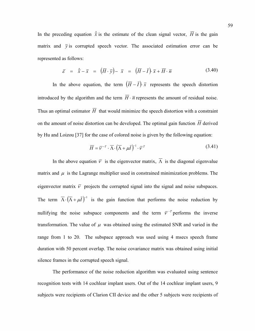
59
In the preceding equation x is the estimate of the clean signal vector, H is the gain
matrix and y is corrupted speech vector. The associated estimation error can be
represented as follows:
( ) ( ) nHxIHxyHxx ⋅+⋅−=−⋅=−= ˆε (3.40)
In the above equation, the term ( ) xIH ⋅− represents the speech distortion
introduced by the algorithm and the term nH ⋅ represents the amount of residual noise.
Thus an optimal estimator H that would minimize the speech distortion with a constraint
on the amount of noise distortion can be developed. The optimal gain function H derived
by Hu and Loizou [37] for the case of colored noise is given by the following equation:
( ) TT IH νµν ⋅+Λ⋅Λ⋅=−− 1 (3.41)
In the above equation ν is the eigenvector matrix, Λ is the diagonal eigenvalue
matrix and µ is the Lagrange multiplier used in constrained minimization problems. The
eigenvector matrix ν projects the corrupted signal into the signal and noise subspaces.
The term ( ) 1−+Λ⋅Λ Iµ is the gain function that performs the noise reduction by
nullifying the noise subspace components and the term T−ν performs the inverse
transformation. The value of µ was obtained using the estimated SNR and varied in the
range from 1 to 20. The subspace approach was used using 4 msecs speech frame
duration with 50 percent overlap. The noise covariance matrix was obtained using initial
silence frames in the corrupted speech signal.
The performance of the noise reduction algorithm was evaluated using sentence
recognition tests with 14 cochlear implant users. Out of the 14 cochlear implant users, 9
subjects were recipients of Clarion CII device and the other 5 subjects were recipients of

60
Clarion S-series device. The Clarion CII device recipients were using the CIS strategy
and the Clarion S-series device recipients were using the SAS strategy. The test material
consisted of HINT sentences corrupted by speech-shaped noise at 5 dB SNR level. The
subjects were tested on sentence recognition with and without using the noise reduction
strategy. The test sentences were delivered via the auxiliary input connection of the
cochlear implant processor. The mean sentence recognition without the use of noise
reduction was about 19%. The mean sentence recognition using the subspace noise
reduction algorithm was significantly greater at 44%.
3.7 Use of amplitude compression in cochlear implants
The compression of envelope amplitudes is an essential component of cochlear implant
(CI) processors because it transforms acoustic amplitudes into electrical amplitudes. This
transformation is necessary because the range in acoustic amplitudes in conversational
speech is considerably larger than the CI patient's electrical dynamic range.
3.7.1 Effect of power law compression on phoneme recognition in cochlear
implants
The logarithmic function is commonly used for compression because it matches the
loudness between acoustic and electrical stimulation and restores the normal loudness
growth. Fu and Shannon [19] studied the effect of varying the power exponent on vowel
and consonant recognition with three cochlear implant listeners. All the three subjects
were recipients of the Nucleus 22 cochlear implant device and were using the SPEAK
strategy. The test material for vowel recognition consisted of 12 vowel stimuli taken from

61
the set created by Hillenbrand et al. [35]. The consonant test material consisted of 16
consonant stimuli. The subjects were tested on a total of 180 vowel tokens, 12 vowels
each spoken by 15 different talkers. For the case of consonant recognition, the subjects
were tested on a total of 96 tokens consisting of 2 repetitions of 16 consonant stimuli
spoken by 3 different talkers. The experiments were conducted using a custom implant
interface system developed by Shannon et al. [73]. The subjects were tested on the
various compression functions using a CIS strategy with four channels of stimulation.
The compression functions were implemented using the following equation:
⎪⎭
⎪⎬
⎫
⎪⎩
⎪⎨
⎧
><<−⋅+<
=
maxmax
maxminminmin
minmin
,,)(
,
AAEAAAAAkEAAE
Eii
ipiii
ii
i
(3.42)
In the above equation iE is the final compressed electric amplitude
corresponding to the uncompressed acoustic amplitude iA , whose dynamic range falls
between .maxmin AandA The power exponent is p and was varied between 0.05, 0.1, 0.15,
0.2, 0.25, 0.3, 0.4, 0.5 and 0.75. The constant ik is chosen so that the compressed output
is iEmax when the input is .maxA
The mean percent vowel recognition score was about 36.8% with a power
exponent value of 0.05. The mean vowel recognition was about 50% for all the power
exponent values ranging from 0.2 to 0.5. The power exponent value of 0.75 resulted in a
drop in mean vowel recognition to about 40.7%. In the case of consonant identification,
the mean percent recognition score was about 56% with a power exponent value of 0.05.
Mean consonant recognition increased to about 70.7% for the power exponent value of
0.2. The power exponent value of 0.75 resulted in a drop in consonant recognition to

62
about 43.5%. The results thus indicate that high vowel and consonant recognition scores
are obtained using the compressed amplitude function, which is in contrast to the linear
amplitude function in normal hearing.
3.7.2 Effect of power exponent variations on consonant recognition in cochlear
implants
Loizou et al. [56] modified the shape of the amplitude mapping functions from strongly
compressive to weakly compressive (nearly linear) by varying the exponent of a power-
law function. Results indicated that, in quiet, the shape of the compression function had
only a minor effect on performance, with the lowest performance obtained for nearly
linear mapping functions.
The subjects for the experiments were four Ineraid cochlear implant users. The
experiments were conducted using a custom laboratory speech processor developed by
Poroy and Loizou [68]. The stimuli were delivered using the CIS strategy. The consonant
test material consisted of 20 consonant stimuli developed at the House Ear Institute [74].
The amplitude compression was performed as per the following equation:
dAcE pii +⋅= (3.43)
In the above equation iE is the compressed electric amplitude corresponding to
the uncompressed acoustic amplitude iA . In the equation c, d are the constants used so
that the electric amplitudes fall within the threshold and most comfortable level. The
power exponent is p which is varied to obtain various compression functions. In the
experiments the power exponent p value was changed between -0.1, -0.0001, 0.2 and 0.6.

63
The mean consonant recognition for all the conditions in which the power exponent was -
0.1, -0.0001 and 0.2 was nearly the same at about 70%. However the mean consonant
recognition dropped to about 40% for the condition in which the power exponent value
was 0.6, which corresponds to a more linear mapping.
3.7.3 Effect of compression on speech perception in noise with cochlear implants
The effect of the shape of the compression function on speech recognition in noise was
investigated by Fu and Shannon [20]. Three Nucleus 22 cochlear implant listeners using
the SPEAK strategy participated in these experiments. The subjects were assessed on
vowel and consonant recognition in presence of speech-shaped noise. The vowel material
consisted of 12 vowel stimuli created by Hillenbrand et al. [35] and the consonant test
material consisted of 16 consonant stimuli. The total vowel test stimuli composed of 180
vowel stimuli consisting of the 12 vowel stimuli each spoken by 15 different talkers. The
total consonant test stimuli consisted of 96 consonant tokens composed of 2 repetitions of
the 16 consonant stimuli each spoken by 3 different talkers.
The experiments were conducted using a custom implant interface system
described by Shannon et al. [73] . The stimuli were delivered to the cochlear implants
listeners using the CIS strategy with 4 channels of stimulation. The compression was
performed in the same way as given by Equation 3.42. The value of minA was set to the
value of noise floor in the absence of speech in all channels. The value of maxA was set to
99 percentile of all amplitude levels in all channels.
The experiments were conducted in quiet and in presence of noise at 6 and 0 dB
SNR levels. In each of these cases, the power exponent value was varied between 0.05,

64
0.1, 0.2, 0.4 and 0.8. In quiet for all the conditions in which power exponent was varied
from 0.05 to 2, mean consonant recognition was nearly the same at about 70% and
dropped to about 46% for the case in which the power exponent was 0.8. In the case of
vowel recognition, the mean scores were about 50% for all the cases in which power
exponent varied from 0.05 to 0.4 and dropped to about 41.7% for the case in which the
power exponent was 0.8. However in the presence of noise, both vowel recognition and
consonant recognition declined dramatically for strongly compressive functions. For the
highly compressive function in which the power exponent value was 0.05, in the case of
6 dB SNR condition; vowel recognition dropped by 20% and consonant recognition
dropped by 30% compared to recognition scores in quiet. For the least compressive
function in which the power exponent value was 0.8, in the case of 6 dB SNR condition;
vowel and consonant recognition were nearly the same as in the quiet condition.

65
CHAPTER 4
STRATEGIES FOR IMPROVING MELODY RECOGNITION WITH COCHLEAR IMPLANTS
4.1 Motivation
One of the challenging problems in cochlear implant research field is music perception.
Despite several advancements made in the technology music perception and appreciation
is still lacking among the implant users. Several research studies involving perception of
music in terms of recognition of familiar melodies have reported poor performance [46].
One important task is to investigate what are the factors in the context of cochlear
implants that contribute to music perception in normal hearing. This will give us
important insights into what additional features need to be incorporated into the future
cochlear implant devices to improve music perception.
Research studies clearly indicate that the rhythmic cues are better presented by the
current implant devices than the melodic cues. Better representation of pitch structure and
melodic elements is lacking in the current devices. One of main reasons for low pitch
perception with the cochlear implant processors is the filter spacing employed in the
current devices. Most of the cochlear implant processors use logarithmic filter spacing in
the frequency range from 300-6000 Hz. Other filter spacing such as the equivalent
rectangular bandwidths ([27], [65]) spacing can potentially be used. While these filter
spacings are highly suitable for speech perception, they are not suitable for music
perception. One of the obvious disadvantages is that musical notes below middle C (262

66
Hz) will not be represented. Another disadvantage is the large filter bandwidths for low
frequency portion (<3 kHz). The filter bandwidths are significantly greater than the
musical semitone steps that quantify the various note positions on the keyboard. A direct
consequence is that distinguishing between adjacent notes on the keyboard might be
highly difficult using the current implant processors. Hence low level of melody
recognition with only the aid of predominantly pitch cues is not surprising.
As a first step forward in this direction, in the current work we investigate the
effect of using new filter spacing with filter bandwidths corresponding to the musical
semitone steps calculated based on the melodic center of gravity of the musical notes
employed in the experiment. We call this filter spacing ‘Semitone filter spacing’ since the
filter band widths are in proportion to the semitone steps on the musical scale.
In the current work, we investigate the effect of filter spacing on melody
recognition in a systematic manner. We experiment with different types of filter spacing
using cochlear implant simulations with normal hearing listeners using noise-band
synthesis as described by Shannon et al. [75]. We attempt to find the minimum number of
filters (2, 4, 6 or 12) based on semitone filter spacing that are sufficient to obtain nearly
asymptotic performance in melody recognition. We also investigate the effect of using a
low frequency bandwidth versus a large frequency bandwidth for melody recognition.
Using a low frequency bandwidth entails more filters in the low frequency region more
important for melody recognition and hence better performance is expected.
Another problem with pitch perception using cochlear implants is the place
mismatch due to the limitations in the electrode array design and corresponding insertion
depths. Oxenham et al. [62] reported that frequency up-shifting can severely affect pitch

67
perception. We also investigate the effect of place mismatch on melody recognition using
frequency up-shifting of simple melodies processed using the semitone filter spacing in
normal hearing. Finally we investigate the effect of the ‘Semitone filter spacing’
strategies on melody recognition by cochlear implant users. The proposed semitone filter
spacing yields filter bands that are primarily located in the low frequency region (<1 kHz)
due to the musical notes employed in the experiments. Hence, we also investigate the
effect of using a hybrid strategy. The hybrid filter spacing employs the narrow semitone
spaced filters in the low-frequency regions and the broad logarithmic filters in the high
frequency region.
In section 4.2 we first investigate the effect of filter spacing, relative phase, carrier
frequency and phase perturbation on melody recognition in a systematic manner in
acoustic hearing. In section 4.3 we investigate the effect of two new filter spacing
strategies, one being the semitone based filter spacing and the other being a hybrid
strategy, to improve music appreciation with cochlear implants.
4.2 Investigation of various factors affecting music perception
In most of the current implants the filter spacing being used is not suitable for music
perception. In the section 4.2.1, we investigate the effect of filter spacing on melody
recognition in acoustic hearing. In section 4.2.2 we investigate the effect of spectral
shifting on melody recognition using the semitone spaced filter structure. In section 4.2.3
we study the effect of relative phase on melody recognition. In section 4.2.4 we study the
effect of carrier frequency on melody recognition. Finally in section 4.2.5 we investigate
the effect of phase perturbation on melody recognition.

68
4.2.1 Effect of filter spacing on melody recognition in acoustic hearing
The perception of common melodies from which the rhythm cues were removed was
investigated using a new filter spacing corresponding to musical semitone structure with
normal-hearing listeners. A noise-band synthesis was performed where analysis and
synthesis filter spacings were varied in steps of a semitone scale based on center of
gravity of melodic information (Kasturi and Loizou [41]). For comparison purposes a
noise-band synthesis using a conventional logarithmic spacing was performed, while
varying the bandwidth. In one scenario, a large bandwidth (300-10525 Hz) was used, and
in another case a smaller bandwidth (225-4500 Hz) was employed. Melody recognition
was evaluated for the three different filter spacings as a function of spectral resolution
using various numbers of channels (2, 4, 6, 12 and 40).
4.2.1.1 Experimental Method
A. Subjects
Ten normal-hearing listeners participated in this experiment. All subjects were native
speakers of American English. The subjects were paid for their participation. All ten
subjects participated in melody recognition experiments using semitone spacing and
logarithmic spacing with large bandwidth. Five subjects participated in the melody tests
using logarithmic spacing with smaller bandwidth.
B. Test Material
A set of 34 simple melodies (e.g., “Twinkle Twinkle”, “Old McDonald”) with all rhythm
information removed was used (Hartmann and Johnson [34]). Melodies consisted of 16

69
equal-duration notes synthesized using samples of a grand piano. The melodic center of
gravity for each tune was concert A (440 Hz) plus or minus a semitone. The largest
difference between the highest and lowest notes was 12 semitones. Subjects were asked
to select 10 melodies they were familiar with.
C. Signal Processing
Test material was first low-pass filtered using a sixth order elliptical filter with a cut-off
frequency of 6000 Hz. Filtered speech was passed though a pre-emphasis filter with a
cut-off frequency of 2000 Hz. This was followed by band-pass filtering into N frequency
bands (where N varied from 2, 4, 6, 12 and 40) using sixth-order Butterworth filters
respectively. The filter bank design using semitone spacing is presented next.
Semitone based filter structure
The semitone based filter bank was designed by using narrow filters that roughly
corresponded to semitone increments with reference to the melodic center of gravity of
the musical notes employed. Number of channels varied was from 2 to 12 with the
following filter bandwidths. For 2-channel case, each filter had a bandwidth of 6
semitones. The filter edges for the two filters are depicted in Table 4.1. For 4-channel
case, each filter had a bandwidth of 3 semitones. The filter edges for the four filters are
depicted in Table 4.2. For 6-channel case, each filter had a bandwidth of 2 semitones.
The filter edges for the six filters are shown in Table 4.3. For 12-channel case, each filter
had a bandwidth of 1 semitone as depicted in Figure 4.1. The filter edges are shown in
Table 4.4.

70
Table 4.1. The 3-dB frequency boundaries of the 2 bands using semitone spacing with the corresponding center frequencies (Hz) of each band. ___________________________________________________________
Band Lower Upper Center
Frequency (Hz) Frequency (Hz) Frequency (Hz)
________________________________________________________________________________________
________________________________________________________________________________________________________________________________________________________________________________
1 300 424 362
2 424 600 512
___________________________________________________________
Table 4.2. The 3-dB frequency boundaries of the 4 bands using semitone spacing with the corresponding center frequencies (Hz) of each band. ___________________________________________________________
Band Lower Upper Center
Frequency (Hz) Frequency (Hz) Frequency (Hz)
________________________________________________________________________________________
________________________________________________________________________________________________________________________________________________________________________________
1 300 357 328
2 357 424 391
3 424 505 464
4 505 600 552
___________________________________________________________

71
Table 4.3. The 3-dB frequency boundaries of the 6 bands using semitone spacing with the corresponding center frequencies (Hz) of each band. ___________________________________________________________
Band Lower Upper Center
Frequency (Hz) Frequency (Hz) Frequency (Hz)
________________________________________________________________________________________
________________________________________________________________________________________________________________________________________________________________________________
1 300 337 318
2 337 378 357
3 378 424 401
4 424 476 450
5 476 535 505
6 535 600 567
__________________________________________________________
Table 4.4. The 3-dB frequency boundaries of the 12 bands using semitone spacing with the corresponding center frequencies (Hz) of each band. ___________________________________________________________
Band Lower Upper Center
Frequency (Hz) Frequency (Hz) Frequency (Hz)
________________________________________________________________________________________
________________________________________________________________________________________________________________________________________________________________________________
1 300 318 309
2 318 337 327
3 337 357 347

72
Table 4.4 - Continued.
4 357 378 367
5 378 400 389
6 400 424 412
7 424 449 437
8 449 476 463
9 476 505 490
10 505 535 520
11 535 566 550
12 566 600 583
___________________________________________________________
Figure 4.1. The filter spacing using 12 channels of semitone spacing.
200 400 600 800 1000 1200
-25
-20
-15
-10
-5
0
Frequency (Hz)
Mag
nitu
de (d
B)
Semitone spacing for 12 channels

73
Conventional logarithmic filter structure
For the conventional logarithmic filter design the number of frequency bands was varied
from 2, 4, 6, 12, and 40. For the large bandwidth conditions, the filters were designed to
span the frequency range from 300 to 10525 Hz in a logarithmic fashion as depicted in
Figure 4.2. The corresponding filter edges for the 12-channel case are shown in Table
4.5. For the small bandwidth conditions, the filters were designed to span the frequency
range from 225 to 4500 Hz in a logarithmic fashion as depicted in Figure 4.3. The filter
edges for the 12-channel case are depicted in Table 4.6.
Figure 4.2. The filter spacing using 12 channels of log spacing with large bandwidth.
1000 2000 3000 4000 5000 6000 7000 8000 9000 10000 11000
-20
-15
-10
-5
0
Frequency (Hz)
Mag
nitu
de (d
B)
Large bandwidth logarithmic spacing for 12 channels

74
Figure 4.3. The filter spacing using 12 channels of log spacing with small bandwidth.
Table 4.5. The 3-dB frequency boundaries of the 12 bands using large bandwidth logarithmic spacing with the corresponding center frequencies (Hz) of each band. ___________________________________________________________
Band Lower Upper Center
Frequency (Hz) Frequency (Hz) Frequency (Hz)
________________________________________________________________________________________
________________________________________________________________________________________________________________________________________________________________________________
1 300 404 352
2 404 543 473
3 543 730 636
0 1000 2000 3000 4000 5000 6000 7000 8000 9000 10000
-20
-15
-10
-5
0
Frequency (Hz)
Mag
nitu
de (d
B)
Small bandwidth logarithmic spacing for 12 channels

75
Table 4.5 - Continued.
4 730 982 856
5 982 1321 1152
6 1321 1777 1549
7 1777 2390 2084
8 2390 3215 2803
9 3215 4325 3770
10 4325 5817 5071
11 5817 7825 6821
12 7825 10525 9175
___________________________________________________________
Table 4.6. The 3-dB frequency boundaries of the 12 bands using small bandwidth logarithmic spacing with the corresponding center frequencies (Hz) of each band. ___________________________________________________________
Band Lower Upper Center
Frequency (Hz) Frequency (Hz) Frequency (Hz)
________________________________________________________________________________________
________________________________________________________________________________________________________________________________________________________________________________
1 225 289 257
2 289 371 330
3 371 476 423
4 476 611 543
5 611 784 697

76
Table 4.6 - Continued.
6 784 1006 895
7 1006 1292 1149
8 1292 1658 1475
9 1658 2128 1893
10 2128 2731 2430
11 2731 3506 3119
12 3506 4500 4003
___________________________________________________________
A noise-band synthesis was performed using the various filter band conditions.
The output of each channel was passed through a rectifier followed by a second order
Butterworth low-pass filter with a center frequency of 120 Hz to obtain the envelope of
each channel output. The rectified output of each channel was modulated with white
noise and finally the melodies were synthesized by summing up the outputs of all the
channels. A block diagram of the noise band synthesis is shown in Figure 4.4.
D. Procedure
The experiments were performed on a PC equipped with a Creative Labs SoundBlaster
16 soundcard. Stimuli were played to the listeners monaurally through Sennheiser HD
250 Linear II circumaural headphones. The names of the melodies were displayed on a
computer monitor, and a graphical user interface enabled the subjects to indicate their
response. Prior to the test, each subject was asked to select ten familiar tunes from the
list of thirty-four melodies. A pilot test session with the ten selected melodies, six

77
repetitions each, was performed using the original unprocessed melodies. It was
mandatory for the subject to score above 90 percent with unprocessed melodies to
participate in the experiment.
Figure 4.4. A block diagram representation of noise band simulation.
After the pilot sessions, the subjects were tested with the melodies processed
through the various conditions of filter spacings using different number of channels. All
the ten subjects were tested on semitone spacing and logarithmic spacing with large
bandwidth. The order of test conditions was partially counterbalanced between subjects.
In a separate session, five of the ten subjects were tested on the conditions with
logarithmic spacing with small bandwidth. Again the order of test conditions was
randomized from subject to subject.
Pre-emphasis
LPF
BPF 1
BPF 2
BPF n
LPF + Rectifier
LPF + Rectifier
LPF + Rectifier
BPF 1
BPF 2
BPF n
White noise
White noise
White noise
Output
Input

78
4.2.1.2 Results and Discussion
(a) Effect of Filter Spacing: Semitone Spacing versus Log Spacing
The mean percent correct scores for melody recognition for the semitone filter spacing
and logarithmic spacing with large bandwidth, are depicted in Figure 4.5, as a function
of number of spectral channels. The standard errors of mean bars are shown along with
the mean recognition scores.
Figure 4.5. Effect of filter spacing: Semitone Spacing versus Log Spacing on melody recognition as a function of number of spectral channels. Two-way ANOVA (repeated measures) indicated a significant effect of spectral
resolution (number of channels), a significant effect of frequency spacing and a
significant interaction (p<0.005). For semitone-spacing Post-hoc tests (Fisher’s LSD)
showed that performance asymptoted (p>0.5) with 4 channels. Performance with 4
channels based on semitone filter spacing was as good as performance with 12 channels
based on logarithmic filter spacing.
0 10 20 30 40 50
60 70 80 90
100
0 5 10 15 20 25 30 35 40
Number of channels
Perc
ent c
orre
ct
Log spacing
Semitone spacing

79
(b) Effect of Signal Bandwidth: Log Spacing with Large Bandwidth versus Log
Spacing with Small Bandwidth
The mean percent correct scores for melody recognition using logarithmic spacing with
small bandwidth, while varying the number of frequency bands are presented in Figure
4.6. The results with semitone spacing and logarithmic spacing with large bandwidth are
also shown for comparison purposes. The standard errors of mean bars are shown along
with the mean recognition scores.
Two-way ANOVA (repeated measures) indicated a significant effect of spectral
resolution (number of channels), a significant effect of bandwidth and a significant
interaction (p<0.005). Post-hoc tests (Fisher’s LSD) indicated that for the 4-channel case,
performance with log spacing using small bandwidth was significantly greater than that
with log spacing using large bandwidth (p=0.013). For the 6-channel case, performance
with semitone spacing was significantly greater than that with log spacing using small
bandwidth (p=0.029). Performance with log spacing using small bandwidth was better
than that with log spacing using large bandwidth (p<0.005).
C. Discussion
The results clearly demonstrate that filter spacing is extremely important for melody
recognition. Using the semitone filter spacing with just 4 channels nearly perfect melody
recognition was achieved. This clearly indicates that the correct frequency placement of
the filters is more important for melody recognition than speech recognition.

80
Figure 4.6. Effect of Signal Bandwidth: Log Spacing with Large Bandwidth versus Log Spacing with Small Bandwidth on melody recognition as a function of number of spectral channels.
The temporal envelope of speech signal has sufficient information for perception
with reduced spectral cues (Shannon et al. [75]). But that is clearly not the case for
melody recognition. For simple melodies the temporal envelope does not provide enough
information for melody identification. Smith et al. [77] reported that the envelope cues
provide insufficient information for melody identification and fine structure cues are
more important. Most crucial information needed for melody identification is coded in
the frequency variations of various notes and pitch contour (Moore and Rosen [60]).
Hence using a large number of channels does not necessarily result in better
melody recognition if the frequency placement of filters is incorrect. Since pitch of
0
10 20
30
40 50
60
70
80 90
100
0 5 10 15 20 25 30 35 40
Number of channels
Perc
ent c
orre
ctLog spacing - Large BWLog spacing - Small BWSemitone spacing

81
complex tones is determined to a large extent by spectral analysis (Hartmann [33]). The
results indicate that the performance with 4-channel semitone spacing is as good as 12-
channel logarithmic spacing. Hence using fewer number of filters but that were more
optimally placed lead to a dramatic increase in melody recognition. The semitone spaced
filters better code the fine structure information and hence better melody recognition is
achieved. For the simple melodies we used in this experiment four optimally placed
filters were sufficient for nearly perfect identification.
The results from experiments by varying the signal bandwidth provide further
evidence that spectral cues are more important than temporal cues for melody
identification. By using a small signal bandwidth (4500 Hz) more filters fall into the low
frequency region corresponding to the majority of note frequencies in the melodies. This
results in better spectral analysis of the melodic frequency content and hence better
recognition when compared to using a large signal bandwidth (10 kHz). For the 4-
channel case, the performance with small signal bandwidth is nearly twice than the
performance with large signal bandwidth.
Hence when a small number of channels are available, which is usually the case
with cochlear implant users (Fishman et al. [17]) using a small bandwidth with log
spaced filters can bring significant benefits to melody recognition. More optimally placed
filters as obtained using the semitone filter spacing can dramatically increase melody
identification.

82
4.2.2 Effect of Spectral shift on melody recognition in acoustic hearing
In the present experiment, we investigate the effect of upward spectral shift on the
identification of simple melodies. The motivation for this experiment was to study the
effect of tonotopic shift due to the inherent place/mismatch in the cochlear implants on
the semitone filter spacing. The spectral shift was introduced by changing the frequency
band width of synthesis filters with respect to the analysis filters. The spectral shift was
studied using a four channel synthesis that simulated the effect of a basal shift of 6.46
mm along the length of the cochlea using the semitone spacing (Kasturi and Loizou [42]).
The same experiments with spectral upward shift were also done with a logarithmic
spacing for comparison purposes.
4.2.2.1 Experimental Method
A. Subjects
Five normal-hearing listeners participated in this experiment.
B. Test Material
The test material was the same as in Experiment 4.2.1.
C. Signal Processing
The un-shifted conditions for the logarithmic spacing used a narrow filter band width
ranging in frequency from 50 to 4000 Hz which is the same filter structure used by Rosen
et al. [70]. This is referred to as ‘Log2’ spacing and corresponding filter edges are shown
in Table 4.7. In the un-shifted condition, the log spacing with large bandwidth as

83
described in Experiment 4.2.1 was also used and is referred to as ‘Log1’ spacing for
comparison. The methodology for signal processing in the un-shifted conditions for
semitone spacing using 4 spectral channels was the same as that described in Experiment
4.2.1. The spectral up-shifting experiments were performed using the Log2 and Semitone
filter spacings by changing the synthesis filters.
For the spectrally shifted conditions, the analysis filters were the same as in un-
shifted condition but the synthesis filter edges were altered. The signal processing used to
simulate the spectral shift is the same as that described by Rosen et al. [70]. The
relationship between the frequency ‘f’’ and the distance ‘d’ along the cochlea is given by
the following equation:
)110(4.165 *06.0 −⋅= df (4.1)
In the above equation the frequency is in Hertz and the distance is in millimeters.
The basal upward shifts of 6.46 mm were simulated by increasing the distance by 6.46
and using the resulting shifted frequencies to generate the altered synthesis filter edges as
given by the following equations:
46.6+= dd (4.2)
)110(4.165 *06.0 −⋅= df (4.3)
The filter edges for the spectrally shifted conditions using the ‘Log2 – shifted’ and
‘semitone – shifted’ filters are shown in Table 4.8 and Table 4.9 respectively.
D. Procedure
The experimental procedure was the same as that described in Experiment 4.2.1.

84
Table 4.7. The 3-dB frequency boundaries of the 4 bands using logarithmic spacing (Log2) with the corresponding center frequencies (Hz) of each band. ___________________________________________________________
Band Lower Upper Center
Frequency (Hz) Frequency (Hz) Frequency (Hz)
________________________________________________________________________________________
________________________________________________________________________________________________________________________________________________________________________________
1 50 286 168
2 286 782 534
3 782 1821 1302
4 1821 4000 2911
___________________________________________________________
Table 4.8. The 3-dB frequency boundaries of the 4 bands with spectral up-shifting using logarithmic spacing (Log2 - shifted) with the corresponding center frequencies (Hz). ___________________________________________________________
Band Lower Upper Center
Frequency (Hz) Frequency (Hz) Frequency (Hz)
________________________________________________________________________________________
________________________________________________________________________________________________________________________________________________________________________________
1 360 937 649
2 937 2147 1542
3 2147 4684 3416
4 4684 10000 7342
___________________________________________________________

85
Table 4.9. The 3-dB frequency boundaries of the 4 bands with spectral up-shifting using semitone spacing (semitone - shifted) with the corresponding center frequencies (Hz) of each band. ___________________________________________________________
Band Lower Upper Center
Frequency (Hz) Frequency (Hz) Frequency (Hz)
________________________________________________________________________________________
________________________________________________________________________________________________________________________________________________________________________________
1 971 1110 1041
2 1110 1273 1192
3 1273 1471 1372
4 1471 1703 1587
___________________________________________________________
4.2.2.2 Results and discussion
The mean percent correct scores for melody recognition are depicted in Figure 4.7, for
the various conditions in the experiment. The standard errors of mean bars are shown
along with the mean recognition scores. ANOVA (repeated measures) indicated a
significant effect [F(4,20)=84.6, p<0.0005] of the various conditions used for processing
on melody recognition. For both the un-shifted and spectrally shifted conditions, post hoc
tests as per Tukey indicated that performance with Semitone spacing was significantly
(p<0.0005) better than Log1 and Log2 filter spacings. Post hoc tests as per Tukey also
indicated that performance with ‘Semitone - shifted’ condition was the same as the
performance with ‘Semitone’ condition (p=1).

86
Figure 4.7. Effect of upward spectral shift on melody recognition using semitone filter spacing with four channels.
One of the inherent problems for pitch perception with cochlear implants is the
place mismatch due to the limitations in electrode insertion mechanism. Several
researchers have attempted to study this effect using frequency transposed or spectrally
up-shifted stimuli (Dorman et al. [11]). It has been demonstrated that spectral up-shifting
has negative impact on speech identification. Fu et al. [21] reported that the upward
spectral shifts of about 6 mm did not severely degrade the recognition of vowels. Not
much research has been done to study the effect of spectral shifting on simple melodies.
It was of interest to investigate the effect of spectral shifts of similar magnitude on
melody recognition using the semitone filter spacing. The results show that the semitone
filter spacing is not significantly affected by basal upward shifts of about 6 mm.
0 10 20 30 40 50 60 70 80 90
100
Log1 Log2 Log2 - shifted Semitone Semitone - shifted
Conditions
Perc
ent c
orre
ct

87
4.2.3 Effect of relative phase on melody recognition in acoustic hearing
The perception of common melodies from which the rhythm cues were removed was
investigated for different phase conditions using normal-hearing listeners. Three different
phase conditions, where the phases were either set to zero, randomly chosen or estimated
using the FFT, namely zero phase, random phase and Fourier phase respectively, were
used to synthesize the melodies. A noise-band synthesis was also performed for
comparison purposes with the random phase condition. For each phase condition as well
as noise-band condition, melody recognition was evaluated as a function of spectral
resolution using various numbers of channels (1, 2, 3, 4, 5, 6, 8, 16 and 32) for synthesis.
4.2.3.1 Experimental Method
A. Subjects
Eighteen normal-hearing listeners (20 to 35 years of age) participated in this experiment.
The subjects were formed into two groups a) ‘Music-informed’ and b) ‘Music-naïve’,
according to their training and background in music. Ten subjects who received five or
more years of training in music were grouped into Music-informed group. Other eight
subjects received less than three years of training in music and were grouped into Music-
naïve group. All subjects were native speakers of American English. The subjects were
paid for their participation.
B. Test Material
Subjects were tested on melody recognition. The melody test used thirty-four common
melodies each consisting of sixteen isochronous notes as used by Hartmann and Johnson

88
[34]. Isochronous notes were used to remove the rhythm cues from the melodies. The
notes were synthesized using samples of acoustic grand piano available with Midi
Software.
C. Signal Processing
Test material was first low-pass filtered using a sixth order elliptical filter with a cut-off
frequency of 6000 Hz. Filtered speech was passed though a pre-emphasis filter with a
cut-off frequency of 2000 Hz. This was followed by band-pass filtering into N
logarithmic frequency bands (where N varied from 1, 2, 3, 4, 5, 6, 8, 16 and 32) using
sixth-order Butterworth filters respectively. The filters were designed to span the
frequency range from 300 to 5500 Hz in a logarithmic fashion. The output of each
channel was passed through a rectifier followed by a second order Butterworth low-pass
filter with a center frequency of 120 Hz to obtain the envelope of each channel output.
Corresponding to each channel a sinusoid was generated with frequency set to the center
frequency of the channel and with amplitude set to the root-mean-squared (rms) energy
of the channel envelope estimated every 4 msecs.
The phase estimation central to this work was performed in three different ways.
The short-term (every 4 msecs) phases were either set to zero, randomly chosen or
estimated using the FFT, henceforth referred to as zero phases, random phases and
Fourier phases respectively. The sinusoids of each band were finally summed and the
level of the synthesized speech segment was adjusted to have the same rms value as the
original speech segment. A block diagram of the sinusoidal synthesis used for the various
phase experiments is shown in Figure 4.8.

89
Figure 4.8. A block diagram representation of sinusoidal synthesis incorporating phase information.
It is worth mentioning that the Fourier phases as used here are a quantized version
of the solution to the sinusoidal phase estimation obtained using the classical Maximum
likelihood estimation [44]. In that sense the Fourier phases represent an optimal solution
for the problem at hand, namely phase estimation and hence better melody recognition is
expected when compared to the other two approaches used to incorporate the phase
information.
A noise-band synthesis was performed for comparison purposes. The stimuli were
filtered using band-pass filters as described earlier. Next the filtered output was half wave
rectified using a low-pass filter with cut-off frequency of 120 Hz. The rectified output of
each channel was modulated with white noise and finally the melodies were synthesized
by summing up the outputs of all the channels.
Pre-emphasis
LPF
BPF 1
BPF 2
BPF n
LPF + Rectifier
LPF + Rectifier
LPF + Rectifier
sin(2πfnt+φn)
Output sin(2πf2t+φ2)
sin(2πf1t+φ1)
Input
RMS1
RMS2
RMSn

90
D. Procedure
The experiments were performed on a PC equipped with a Creative Labs SoundBlaster
16 soundcard. Stimuli were played to the listeners monaurally through Sennheiser HD
250 Linear II circumaural headphones. The names of the melodies were displayed on a
computer monitor, and a graphical user interface was used that enabled the subjects to
indicate their response by clicking a button corresponding to the melody played.
At the beginning of the test, each subject was presented with the full list of thirty-
four melodies and asked to pick ten tunes the subject was familiar with. A pilot test
session with the ten selected melodies, six repetitions each, was performed using the
original melodies. It was mandatory for the subject to score above 90 percent with
original melodies to participate in the phase tests. In order to get the subject familiar with
the processed melodies, the subject was next tested with the Fourier phase condition
using sixteen channels for synthesis. Each token was repeated three times and feedback
was provided. Again, it was mandatory for the subject to score above 90 percent to
participate in the phase tests.
After the pilot sessions, the subjects were tested with the phase manipulated
stimuli. In each test the subject was tested for four conditions that included the three
phase conditions namely zero phase, random phase and Fourier phase as well as the
noise-band synthesis. For each condition the subject was tested for different number of
channels ranging from 1, 2, 3, 4, 5, 6, 8, 16 and 32 in a random order. Each token was
repeated six times and no feedback was provided during the test. The order of the four
conditions was randomized from subject to subject. Thus each subject was tested for a
total of 36 conditions incorporating 4 conditions and 9 channel combinations for each

91
phase condition. The purpose of the experiment was two-fold. The first motivation was to
determine if the melody recognition varied with the different phase manipulations and if
so to what extent. The second motivation was to assess how many channels were required
to obtain nearly perfect recognition of melodies for each phase condition.
4.2.3.2 Results and Discussion
The mean percent correct scores for the different phase conditions for subjects with
musical background are shown in Figure 4.9 and for subjects with no musical
background in Figure 4.10. The standard errors of mean bars are shown along with the
mean recognition scores.
0
10
20
30
40
50
60
70
80
90
100
1 2 3 4 5 6 8 12 16 32
Number of channels
Perc
ent c
orre
ct
Fourier phaseZero phaseRandom phaseNoise band
Figure 4.9. Effect of relative phase on melody recognition for music informed subjects.

92
Statistical analysis showed a significant effect of the phase on melody
recognition. Poor performance was obtained with zero phases showing no benefit in
melody identification with increasing number of channels. Performance with random
phases improved with increasing number of channels, consistent with the performance
obtained with noise-band simulations. Best performance was obtained with the Fourier
phases. Three channels were sufficient in achieving perfect melody identification.
Two-channel condition however showed a significant drop in performance which
can be attributed to the nature of frequency information available in that case. The
dependence of the performance in melody recognition task on the center frequencies of
the frequency bands used for synthesis is discussed in the following experiment.
0
10
20
30
40
50
60
70
80
90
100
1 2 3 4 5 6 8 12 16 32
Number of channels
Perc
ent c
orre
ct
Fourier phaseZero phaseRandom phaseNoise band
Figure 4.10. Effect of relative phase on melody recognition for music naïve subjects.

93
We first discuss the results on melody recognition with the ‘Music informed’
subjects. Statistical analysis using Fisher’s LSD showed that performance on melody
recognition peaked using just 3 channels with the Fourier phase condition (p>0.5). For
the case of noise-band synthesis performance on melody recognition asymptoted using 16
channels. Using the random phase condition, 32 channels were required to reach
asymptotic performance. For the zero phase condition, performance on melody
recognition did not asymptote even with 32 channels.
For the 6-channel case, the performance with the noise-band synthesis was
significantly lower than that with the Fourier phase condition (p=0.011). The
performance with the random phase condition was significantly less than that with the
noise-band synthesis (p=0.011). Finally the performance with the zero phase condition
was significantly lower than that with the random phase condition (p<0.0005).
For the 16-channel case, the performance on melody recognition using the noise-
band synthesis was the same as that with the Fourier phase condition (p=0.477). The
performance with random phase condition was significantly lower than that with the
Fourier phase condition (p=0.001). Finally the performance with the zero phase condition
was significantly lower than the random phase condition (p<0.0005).
Next we discuss the results with ‘Music naïve’ subjects. Statistical analysis using
Fisher’s LSD showed that performance asymptoted with Fourier phase using 3 channels
(p>0.5). For the case of noise-band synthesis, performance on melody recognition
asymptoted with 32 channels. For the case of random phase and zero phase conditions,
performance on melody recognition did not asymptote even with using 32 channels.

94
These results clearly show that the coding of phase information has a significant impact
on melody recognition.
For the 6-channel case, the performance on melody recognition with the noise-
band synthesis was significantly lower than the performance with the Fourier phase
condition (p<0.0005). The performance on melody recognition with the random phase
condition was not significantly different than the performance with noise-band synthesis
(p=0.096). Finally the performance on melody recognition using the zero phase
condition was not significantly different than the performance with the random phase
condition (p=0.473).
For the 16-channel case, the performance on melody recognition with noise-band
synthesis was significantly lower than the performance with the Fourier phase condition
(p<0.0005). The performance on melody recognition with the random phase condition
was significantly lower than the performance with noise-band synthesis (p=0.019). The
performance on melody recognition with zero phase condition was not significantly
different than the performance with the random phase condition (p=0.249).
Statistical analysis comparing the performance on melody recognition with the
Music informed subjects and the Music naïve subjects showed that musical background
had a significant effect on melody recognition with noise-band synthesis and random
phase condition. Musical background did not have a significant effect on melody
recognition with Fourier phase and zero phase conditions. Mean melody recognition for
the music informed subjects was significantly greater than that for the music naïve
subjects for noise-band synthesis for 16-channel condition (p=0.002) and 6-channel
condition (p<0.0005). Performance on melody recognition with the Music informed

95
subjects was significantly greater than that with the music naïve subjects for the random
phase condition for 32-channel case (p=0.007), 16-channel case (p=0.001) and 6-channel
case (p<0.0005).
These results indicate that addition of the phase information as provided by the
Fourier phase significantly improves the performance on melody recognition when
compared to that in the absence of the phase information as in zero phase condition.
These results are again in agreement with the findings of Smith et al. [77] that fine
structure information is more important for pitch perception. In their studies they extract
envelope and fine structure information using the Hilbert transform in each channel. They
created auditory chimeras in which the signal is composed of envelopes cues
corresponding to one melody and fine structure cues corresponding to another melody.
The subjects were tested on melody recognition based on the auditory chimeras presented
to them. For the case of fewer number of channels (<16) the fine structure information
was found to be more important than the envelope information. This is consistent with
the high melody recognition scores obtained using the Fourier phase condition for smaller
number of channels. As the number of channels is increased (>32) they observed that
envelope cues dominate the fine structure cues. This is again consistent with the fact that
melody recognition with random phase conditions is close to Fourier phase condition for
the 32-channel case.
Kong et al. [47] investigated the effect of combining the fine structure
information and the envelope information on melody recognition. In their studies they
used frequency modulation cues to incorporate the fine structure information. They did
melody recognition experiments with normal hearing listeners to assess the importance of

96
frequency modulation information. With the addition of the frequency modulation cue
nearly perfect melody recognition was achieved using 4 channels for synthesis. This is
again in agreement with the results obtained with the Fourier phase conditions.
de Cheveigne [9] discusses the use of a cancellation model for pitch perception
which is also sensitive to phase. The cancellation models can account for the perception
of multiple pitches evoked by concurrent harmonic sounds as in the case of common
musical pieces. The cancellation model based on subtraction in time building block and is
highly sensitive to phase. Computer generated models for the auditory periphery by
Meddis and Hewitt ([58], [59] ) use hair cell transduction stages that introduce phase
sensitivity. Thus incorporation of phase information into the electrical stimulation for
cochlear implants can benefit music perception.
4.2.4 Effect of carrier frequency for synthesis on melody recognition in acoustic
hearing
This experiment assessed the effect of frequency bands employed in synthesis on the
melody recognition. Melodies were synthesized using a single channel and two channels
and performance was measured by varying the center frequencies of the filters employed
in the synthesis. Questioning whether the single-channel performance was sensitive to the
frequency of the sine wave, we conducted an experiment in which the sine wave
frequency was varied from 250 to 1000 Hz. Similarly for two-channel condition, two
different sets of center frequencies were employed.

97
4.2.4.1 Experimental Method
A. Subjects
Seven normal-hearing listeners (20 to 35 years of age) participated in this experiment.
Four subjects were from Music-informed group and the remaining three from Music-
naïve group. All subjects were native speakers of American English. The subjects were
paid for their participation.
B. Test Material
The test material consisted of thirty-four common melodies as used in Experiment 4.2.3.
C. Signal Processing
All the stimuli were processed in the same way as described in Experiment 4.2.3 using
Fourier phase for the synthesis of melodies. For the single-channel conditions, the signal
processing varied only in the frequency of the sine wave used for synthesis. Four
different conditions of single-channel synthesis were generated using sine wave
frequencies of 250, 500, 750 and 1000 Hz respectively. For the two-channel cases, two
different sets of frequency bands were employed. In first case, the center frequencies for
the two channels were 792 and 3400 Hz respectively. In the second case the center
frequencies were 500 and 3400 Hz respectively. However, the two bands were not
continuous and there was a hole from 700 to 1284 Hz in between the two bands.

98
D. Procedure
The general experimental procedures were the same as in Experiment 4.2.3. The subjects
were tested on four conditions spanning different sine wave frequencies for single cannel
synthesis and two conditions for the two-channel synthesis. Thus each subject was tested
on a total of six conditions. During the test, each token was repeated six times and no
feedback was provided during the test.
4.2.4.2 Results and Discussion
The mean percent correct scores (along with the standard errors of mean) for the single-
channel conditions versus the sine wave frequency are shown in Figure 4.11.
Figure 4.11. Effect of carrier frequency for synthesis on melody recognition for single-channel case.
0
20
40
60
80
100
250 500 750 1000
Center frequency (Hz)
Perc
ent c
orre
ct
Music naive
Music informed

99
Statistical analysis using Fisher’s LSD indicated a significant effect of the sine
wave frequency, with a peak in performance obtained at 500 Hz (p<0.05). Perfect melody
identification was obtained using a single sine wave with frequency set to 500 Hz. No
significant difference in performance on melody recognition using sine wave frequencies
of 250, 750 and 1000 Hz was observed (p>0.5).
The mean percent correct scores for the two-channel conditions are plotted versus
the center frequency of the first channel, since the second channels were identical in both
the conditions. The results for the two-channel conditions are shown in Figure 4.12. The
standard errors of mean bars are shown along with the mean recognition scores.
Figure 4.12. Effect of carrier frequency for synthesis on melody recognition for two-channel case.
0
20
40
60
80
100
500 800
Center frequency (Hz)
Perc
ent c
orre
ct
Music naive
Music informed

100
Statistical analysis using Fisher’s LSD showed that the performance was
significantly better when the center frequency of the first channel was 500 Hz than when
it was 792 Hz for the Music naïve group (p<0.05). For the Music informed subjects the
performance was not significantly different between 500 and 792 Hz conditions
(p=0.137). The mean performance with 500 Hz condition was greater than the mean
performance with 792 Hz condition, with the mean difference being 19.
These results again signify the importance of frequency place in pitch perception.
A variation in the carrier frequency can result in the wrong place in the auditory
periphery to be excited and can cause problems in pitch perception and hence melody
recognition. Oxenham et al. [63] conducted similar experiments on pitch perception using
frequency transposed stimuli. They conducted frequency discrimination experiments with
pure tones and frequency transposed tones. The performance on frequency discrimination
was relatively poor with frequency transposed stimuli compared to the pure tone stimuli.
The low melody recognition scores obtained with the perturbations in carrier frequency
are in agreement with these results.
4.2.5 Effect of perturbation in phase information on melody recognition in
acoustic hearing
In this experiment we took the next logical step to quantify the amount of perturbation in
phase information that is tolerable for melody recognition in normal hearing listeners.
The optimal phase information as given by Fourier phase was distorted by adding a
random jitter varying from zero to pi degrees in extent and the corresponding melody
recognition was investigated.

101
4.2.5.1 Experimental Method
A. Subjects
Nine normal-hearing listeners participated in this experiment. All subjects were native
speakers of American English. The subjects were paid for their participation.
B. Test Material
The test material consisted of thirty-four common melodies as used in Experiment 4.2.3.
C. Signal Processing
All the stimuli were processed in the same way as described in Experiment 4.2.3 using
Fourier phase and a single channel for the synthesis of melodies. Single channel was used
so as to restrict the number of phase parameters involved in the experiment and to better
identify the effect of phase jitter on melody perception. The signal processing varied only
for the phase estimation. Here a random phase jitter was added to the estimated Fourier
phase. The optimal Fourier phase was perturbed to various levels using 0, 45, 90, 120,
150 and 180 degrees of random jitter to investigate the melody recognition for different
extents of phase perturbation.
D. Procedure
The general experimental procedures were the same as in Experiment 4.2.3. The subjects
were tested for six conditions of phase perturbations where the added random phase jitter
varied from 0, 45, 90, 120, 150 and 180 degrees. The subjects were first tested with the 0
phase jitter condition which served as the baseline. The other five conditions were played

102
in random order from subject to subject. Each token was repeated six times and no
feedback was provided during the test.
4.2.5.2 Results and Discussion
The mean percent correct scores for the different phase jitter conditions are shown in
Figure 4.13. The standard errors of mean bars are shown along with the mean
recognition scores. Melody recognition remained very high till 90 degrees of phase
perturbation. Relatively low recognition scores were obtained for 150 and 180 degrees.
The 50 percent point of melody recognition seems to be somewhere between 120 and 150
degrees.
Figure 4.13. Effect of phase perturbation on melody recognition.
Statistical analysis using Fisher’s LSD indicated that melody recognition scores
were nearly the same for 0, 45 and 90 degrees of phase perturbation (p>0.5). Statistical
0
20
40
60
80
100
120
0 20 40 60 80 100 120 140 160 180 200
Phase perturbation (degrees)
Perc
ent c
orre
ct

103
analysis indicated that melody recognition with 120 degrees of phase perturbation was
significantly lower than that with 90 degrees of perturbation (p<0.0005). Melody
recognition further dropped with 150 and 180 degrees of perturbation compared to 120
degrees of perturbation (p<0.0005). These results again indicate the significant effect of
phase on melody recognition. Moreover it is worth noting that keeping the amplitude
information the same, the phase information can be perturbed to an extent where the
melody can no longer be identified.
4.3 Novel filter spacing techniques for better music perception in electric hearing
In this experiment cochlear implant recipients were tested on melody recognition task
without the aid of rhythm cues, using the conventional log spacing and the semitone
spacing described earlier. The conventional logarithmic spacing was employed using 16
spectral channels and hence 16 stimulation electrodes. The novel semitone spacing was
employed using 4, 6 and 12 spectral bands and correspondingly 4, 6, and 12 stimulation
electrodes. Another filter spacing which incorporated both the narrow semitone filter
spacing and the relatively broad logarithmic spacing was also investigated. The hybrid
filter spacing employed the narrow semitone spaced filters in the low-frequency regions
and the broad logarithmic filters in the high frequency region (Kasturi and Loizou [42]).
4.3.1 Experimental Method
A. Subjects
Six cochlear implant users who were recipients of Clarion CII (Advanced Bionics)
processor participated in this experiment. All the subjects were postlingually deafened

104
adults who used the cochlear implant for a minimum of 2 to 3 years. The biographical
data for the six subjects is presented in Table 4.10.
B. Test Material
The test material consisted of the same melodies with rhythm cues removed that were
used in Experiment 4.2.3.
C. Signal Processing
The test material was first passed through a pre-emphasis filter with a cut-off frequency
of 2000 Hz. This was followed by band-pass filtering in N (4, 6, 12, and 16) channels
using sixth order Butterworth filters. Band-pass filtering was done in three different ways
using three different filter spacings, namely conventional log spacing, semitone filter
spacing and hybrid filter spacing. The filter bank design for each of the different filter
spacing strategies is described later. The channel envelopes for each filter were extracted
using rectification and followed by a low-pass filter with cut-off frequency of 1200 Hz.
The envelope outputs of each channel were compressed using a power-law
function (Loizou et al. [56]) to obtain the amplitudes of stimulation pulses in micro
amperes. The compression of channel outputs was tailored to each cochlear implant
recipient using the individual threshold (THR) and most comfortable level (MCL) values
for that subject. Finally the pulses were delivered to the subject using the continuous
interleaved sampling (CIS) strategy at a rate determined by the subject’s pulse width.

105
Table 4.10. The biographical data for the six cochlear implant subjects.
Subject Gender Age at the
time of
testing
Years of
experience
using the
cochlear
implant
Percentage
sentence
recognition
in quiet
Probable
cause of
hearing loss
S1 Male 69 4 88 Unknown
S2 Female 49 4 96 Otosclerosis
S3 Female 52 3 93 Unknown
S4 Female 59 3 87 Prescription
drugs
S5 Female 46 4 90 Unknown
S6 Female 38 4 87 Genetics
(adolescent
onset loss)
Incorporation of Various Filter Spacing Strategies
(i) Conventional Logarithmic Spacing Strategy (LOG)
For the conventional logarithmic spacing 16 analysis filters were used spanning the
frequency range 350-5500 Hz in a logarithmic fashion. All the filters were band-pass
filters, except for the last filter (filter 16) which was a high-pass filter as depicted in
Figure 4.14. In this strategy 16 stimulation electrodes were used and the filter edges are
depicted in Table 4.11.

106
Table 4.11. The 3-dB frequency boundaries of the 16 bands for 16LOG strategy with the corresponding center frequencies (Hz) of each band. ___________________________________________________________
Band Lower Upper Center
Frequency (Hz) Frequency (Hz) Frequency (Hz)
________________________________________________________________________________________
________________________________________________________________________________________________________________________________________________________________________________
1 350 416 383
2 416 494 455
3 494 587 540
4 587 697 642
5 697 828 762
6 828 983 906
7 983 1168 1076
8 1168 1387 1278
9 1387 1648 1518
10 1648 1958 1803
11 1958 2326 2142
12 2326 2762 2544
13 2762 3281 3022
14 3281 3898 3590
15 3898 4630 4264
16 4630 11025 -
___________________________________________________________

107
Figure 4.14. The filter spacing using 16 channels of log spacing (16LOG).
(ii) Semitone Spacing Strategies (SM)
For the semitone spacing the analysis filters were varied in semitone steps around the
center of gravity of melodic frequency content. Three strategies namely 4SM, 6SM,
12SM were developed based on semitone spacing.
4SM - First strategy used 4 channels of stimulation. In this strategy four analysis filters as
shown in Table 4.12, based on semitone spacing were used. The 4 most apical electrodes
in the implant were used to deliver the current pulses of stimulation.
1000 2000 3000 4000 5000 6000
-20
-18
-16
-14
-12
-10
-8
-6
-4
-2
0
Frequency (Hz)
Mag
nitu
de (d
B)
Filter spacing for 16LOG strategy

108
6SM - Second strategy used 6 channels of stimulation. Here six analysis filters using
semitone spacing as shown in Figure 4.15 were employed. The 6 most apical electrodes
were used for stimulation. The filter edges are shown in Table 4.13.
12SM - Third strategy employed 12 channels of stimulation. In this case twelve
semitone-spaced analysis filters as depicted in Table 4.14 were employed. The 12 most
apical electrodes were used for the stimulation.
Figure 4.15. The filter spacing using 6 channels of semitone spacing (6SM).
300 350 400 450 500 550 600 650-20
-18
-16
-14
-12
-10
-8
-6
-4
-2
0
Frequency (Hz)
Mag
nitu
de (d
B)
Filter spacing for 6SM strategy

109
Table 4.12. The 3-dB frequency boundaries of the 4 bands for 4SM strategy with the corresponding center frequencies (Hz) of each band. ___________________________________________________________
Band Lower Upper Center
Frequency (Hz) Frequency (Hz) Frequency (Hz)
________________________________________________________________________________________
________________________________________________________________________________________________________________________________________________________________________________
1 311 370 341
2 370 440 405
3 440 523 482
4 523 622 573
___________________________________________________________ Table 4.13. The 3-dB frequency boundaries of the 6 bands for 6SM strategy with the corresponding center frequencies (Hz) of each band. ___________________________________________________________
Band Lower Upper Center
Frequency (Hz) Frequency (Hz) Frequency (Hz)
________________________________________________________________________________________
________________________________________________________________________________________________________________________________________________________________________________
1 311 349 330
2 349 392 371
3 392 440 416
4 440 494 467
5 494 554 524

110
Table 4.13 - Continued.
6 554 622 588
___________________________________________________________
Table 4.14. The 3-dB frequency boundaries of the 12 bands for 12SM strategy with the corresponding center frequencies (Hz) of each band. ___________________________________________________________
Band Lower Upper Center
Frequency (Hz) Frequency (Hz) Frequency (Hz)
________________________________________________________________________________________
________________________________________________________________________________________________________________________________________________________________________________
1 311 329 320
2 329 349 339
3 349 370 360
4 370 392 381
5 392 415 404
6 415 440 428
7 440 460 450
8 460 494 477
9 494 523 509
10 523 554 539
11 554 587 571
12 587 622 605
___________________________________________________________

111
(iii) Hybrid Strategies (SM+LOG)
In the hybrid strategies, both the semitone spaced filters and the logarithmic spaced filters
were used. In the low frequency regions corresponding to the fundamental frequency, the
narrow band semitone filters were employed. The most apical electrodes were used to
deliver the channel envelopes corresponding to these analysis filters. In the high
frequency regions, relatively broad band logarithmic filters were used. All the hybrid
strategies involved 16 channels of stimulation. Three different strategies, namely
4SM+LOG, 6SM+LOG, 12SM+LOG were developed each using different number of
semitone spaced filters and logarithmic spaced filters.
4SM+LOG - In the first strategy, 4 most apical electrodes were stimulated using the
channel envelopes corresponding to 4 semitone spaced filters. The rest 12 electrodes
were stimulated using relatively broad logarithmic spaced filters, whose filter edges are
shown in Table 4.15.
6SM+LOG - In the second strategy, 6 most apical electrodes delivered stimulation
corresponding to the outputs of 6 semitone spaced filters. The rest 10 electrodes were
stimulated using 10 logarithmic filters as depicted in Figure 4.16 and the filter edges are
shown in Table 4.16.
12SM+LOG - In the third strategy, 12 semitone spaced filters were used to stimulate the
most apical 12 electrodes. The rest 4 electrodes were stimulated using 4 logarithmic
filters as shown in Table 4.17.

112
Table 4.15. The 3-dB frequency boundaries of the 16 bands for 4SM+LOG strategy with the corresponding center frequencies (Hz) of each band. ___________________________________________________________
Band Lower Upper Center
Frequency (Hz) Frequency (Hz) Frequency (Hz)
________________________________________________________________________________________
________________________________________________________________________________________________________________________________________________________________________________
1 311 370 341
2 370 440 405
3 440 523 482
4 523 622 573
5 622 734 678
6 734 865 799
7 865 1020 943
8 1020 1203 1112
9 1203 1419 1311
10 1419 1673 1546
11 1673 1973 1823
12 1973 2327 2150
13 2327 2744 2535
14 2744 3236 2990
15 3236 3816 3526
16 3816 4500 4158
___________________________________________________________

113
Table 4.16. The 3-dB frequency boundaries of the 16 bands for 6SM+LOG strategy with the corresponding center frequencies (Hz) of each band. ___________________________________________________________
Band Lower Upper Center
Frequency (Hz) Frequency (Hz) Frequency (Hz)
________________________________________________________________________________________
________________________________________________________________________________________________________________________________________________________________________________
1 311 349 330
2 349 392 371
3 392 440 416
4 440 494 467
5 494 554 524
6 554 622 588
7 622 758 690
8 758 924 841
9 924 1126 1025
10 1126 1373 1249
11 1373 1673 1523
12 1673 2039 1856
13 2039 2485 2262
14 2485 3029 2757
15 3029 3692 3361
16 3692 4500 4096
___________________________________________________________

114
Table 4.17. The 3-dB frequency boundaries of the 16 bands for 12SM+LOG strategy with the corresponding center frequencies (Hz) of each band. ___________________________________________________________
Band Lower Upper Center
Frequency (Hz) Frequency (Hz) Frequency (Hz)
________________________________________________________________________________________
________________________________________________________________________________________________________________________________________________________________________________
1 311 329 320
2 329 349 339
3 349 370 360
4 370 392 381
5 392 415 404
6 415 440 428
7 440 460 450
8 460 494 477
9 494 523 509
10 523 554 539
11 554 587 571
12 587 622 605
13 622 1020 821
14 1020 1673 1347
15 1673 2744 2208
16 2744 4500 3622
___________________________________________________________

115
Figure 4.16. The filter spacing using 16 channels of 6SM+LOG hybrid spacing.
D. Procedure
The cochlear implant subjects were tested using the Clarion research interface-II
(Advanced Bionics). The names of the melodies were displayed on a computer monitor,
and a graphical user interface enabled the subjects to indicate their response.
Melody recognition task
Prior to the test, the subjects were asked to indicate ten known melodies from the list of
melodies. The subjects were given a practice session that lasted for 5 minutes. Following
the practice session, the subjects were tested on the ten selected melodies using the
500 1000 1500 2000 2500 3000 3500 4000 4500 5000-20
-18
-16
-14
-12
-10
-8
-6
-4
-2
0
Frequency (Hz)
Mag
nitu
de (d
B)
Filter spacing for 6SM+LOG strategy
116
logarithmic spacing, semitone spacing and hybrid strategies. The subjects were tested for
a total of seven different strategies. Each strategy was tested in 2 blocks of 3 repetitions.
The order of test melodies was randomized during the presentation of test. The various
strategies were tested in a partially counterbalanced manner from subject to subject.
Melodic preference task
Following the melody recognition test, the subjects participated in the preference test. In
one scenario, the task was to compare the LOG and 6SM strategies. In another scenario,
the task was to compare the LOG and 6SM+LOG strategies. In each presentation of the
test the subjects listened to two tokens, each processed using a particular strategy (A, B).
The melody in both the tokens was the same, but the tokens differed in the processing
strategy. The preference test was done over 10 test pairs using 5 melodies and order of
processing strategies was balanced.
The subjects were instructed to make a preference statement as to which token
sounded more musical and instructed to rate the amount of preference in three levels
(Slightly Better, Better, Much Better). Based on this, 6 (signed) confidence ratings were
assigned and a distance measure was computed as described by Baer et al. [2]. The
percentage preference was computed as the percentage of the number of times token B is
preferred over token A. The percentage preference value ranges from 0 to 100. The
distance measure was computed to measure how much better token B sounded than token
A. For instance the rating, token B is ‘Much Better’ than token A is coded as 3 to
compute the distance measure. On the other hand, the rating token A is ‘Much Better’
than token B is coded as -3 to compute the distance measure. Since distance measure is

117
computed over 10 test pairs, its value ranges from -30 to 30. For a strategy pair (A, B), a
positive value of the distance measure indicates that the strategy A is preferred, and a
negative value indicates otherwise.
4.3.2 Results and Discussion
The mean percent correct recognition scores for melody recognition are depicted for the
different strategies in Figure 4.17. The standard errors of mean bars are shown along
with the mean recognition scores. Individual subject scores are shown in Figure 4.18 -
Figure 4.23 for the comparison of different semitone filter spacing strategies against the
conventional logarithmic spacing strategy.
Figure 4.17. Mean percent correct scores for melody recognition.
0 10 20 30 40 50 60 70 80 90
100
16LOG 4SM 6SM 12SM 4SM+LOG 6SM+LOG 12SM+LOG
Conditions
Perc
ent c
orre
ct

118
Figure 4.18. Individual subject scores for comparison of 16LOG and 4SM strategies.
Figure 4.19. Individual subject scores for comparison of 16LOG and 4SM+LOG strategies.
0 10 20 30 40 50 60 70 80 90
100
S1 S2 S3 S4 S5 S6 Subjects
Perc
ent c
orre
ct
16LOG
4SM
0 10 20 30 40 50 60 70 80 90
100
S1 S2 S3 S4 S5 S6 Subjects
Perc
ent c
orre
ct
16LOG
4SM+LOG

119
Figure 4.20. Individual subject scores for comparison of 16LOG and 6SM strategies.
Figure 4.21. Individual subject scores for comparison of 16LOG and 6SM+LOG strategies.
0 10 20 30 40 50 60 70 80 90
100
S1 S2 S3 S4 S5 S6 Subjects
Perc
ent c
orre
ct
16LOG
6SM
0 10 20 30 40 50 60 70 80 90
100
S1 S2 S3 S4 S5 S6 Subjects
Perc
ent c
orre
ct
16LOG
6SM+LOG

120
Figure 4.22. Individual subject scores for comparison of 16LOG and 12SM strategies.
Figure 4.23. Individual subject scores for comparison of 16LOG and 12SM+LOG strategies.
0 10 20 30 40 50 60 70 80 90
100
S1 S2 S3 S4 S5 S6 Subjects
Perc
ent c
orre
ct
16LOG
12SM
0 10 20 30 40 50 60 70 80 90
100
S1 S2 S3 S4 S5 S6 Subjects
Perc
ent c
orre
ct
16LOG
12SM+LOG

121
The mean recognition (54.79%) with the 12SM strategy was higher than the mean
recognition (41.74%) with the 16LOG strategy. The statistical analysis using Paired-
samples T-test showed that the performance with 12SM strategy was significantly better
than the performance with the 16LOG strategy (p=0.021). The mean recognition with the
6SM strategy was higher than the mean recognition with the 16LOG strategy but the
difference just missed significance (p=0.067). The mean recognition with the 4SM
strategy was better than the mean recognition with the 16LOG strategy but the difference
was not statistically significant (p=0.125).
The mean recognition with the 4SMPLOG strategy was higher than the
performance with the 16LOG strategy but the difference just missed significance
(p=0.075). The performance with the 6SMPLOG strategy was better than the
performance with the 16LOG strategy but the difference just missed significance
(p=0.055). The performance with the 12SMPLOG strategy was better than the
performance with the 16LOG strategy but the difference just missed significance
(p=0.064).
The melody recognition with the various semitone spacing strategies 4SM, 6SM
and 12SM was nearly the same which is consistent with the result in Experiment 4.2.1
that performance with 4 channels semitone filter spacing was the same as that with 12-
channel semitone filter spacing. The melody recognition with the hybrid strategies was
nearly the same as that with the semitone spacing strategies, which indicates that the
addition of high frequency channels (presenting overtone information) did not result in
additional benefit at least for the melodies employed in this experiment. This is analogous
to the common observation in normal hearing that higher order harmonics do not

122
contribute much to the pitch percept [37]. Other possible reasons might be the limited
number of available frequency channels and frequency/place mismatch in the cochlear
implants
The percentage preference results in terms of the number of selections or positive
ratings are depicted in Table 4.18 for 16LOG versus 6SM comparison and 16LOG versus
6SMPLOG comparison. The results indicated that the semitone filter spacing strategies
were preferred over the logarithmic spacing strategy. The mean preference score was
96.67% for the 6SM strategy over the 16LOG strategy. The mean preference score was
58.33% for the 6SMPLOG over the 16LOG strategy.
Table 4.18. The percent preference scores for semitone filter spacing strategies over conventional logarithmic spacing strategy.
% preference S1 S2 S3 S4 S5 S6 Mean
16LOG Vs 6SM 100 100 100 90 90 100 96.67
16LOG Vs
6SM+LOG 100 80 0 20 100 50 58.33
The preference results in terms of the distance measure are depicted in Table 4.19
for 16LOG versus 6SM comparison and 16LOG versus 6SMPLOG comparison. Positive
distance metrics were obtained for both the semitone spacing strategies. For the 6SM
strategy the distance measure was 18.83 over the 16LOG strategy. The distance measure
for the 6SMPLOG strategy was 2.67 for the 6SMPLOG strategy over the 16LOG
strategy. The 6SM semitone spacing strategy was highly preferred over the 16LOG
strategy with mean preference over 95%. This indicates that a small number of optimally
placed filters can increase melodic quality and music appreciation with cochlear implants.

123
Table 4.19. The distance measures for semitone filter spacing strategies over conventional logarithmic spacing strategy. Distance measure S1 S2 S3 S4 S5 S6 Mean
16LOG Vs 6SM 25 20 20 14 14 20 18.83
16LOG Vs
6SM+LOG 12 8 -19 -10 25 0 2.67
This is again consistent with the findings of Smith et al. [77] and Kong et al. [47]
that only a few number of channels with fine structure information are enough for perfect
melody recognition in normal hearing. Results from Experiment 4.2.1 indicated a
significant difference in melody recognition scores between the conventional logarithmic
spacing strategies and semitone based filter spacing strategies. The 6SM strategy
delivered stimulation only to the apical electrodes and was highly preferred over 16LOG
strategy. This indicates that individual frequency note separation and finer encoding of
frequency information is highly essential for melody perception and needs to be
incorporated in the future cochlear implant processors.

124
CHAPTER 5
STRATEGIES FOR BETTER SPEECH PERCEPTION IN NOISE WITH COCHLEAR IMPLANTS
5.1 Motivation
Most noise reduction methods proposed for cochlear implants, including the multi-
microphone methods (Van Hoesel and Clark [82]), are based on pre-processing the noisy
signal and presenting the enhanced signal to the cochlear implant users. The pre-
processing approach has several drawbacks. The first disadvantage is that pre-processing
algorithms sometimes introduce unwanted distortion (e.g., musical noise in spectral
subtractive algorithms [4]) in the signal despite the fact that these algorithms improve the
SNR. The second disadvantage is that pre-processing algorithms can be computationally
complex and do not work synergistically with existing cochlear implant strategies.
Finally, there is no simple approach for optimizing the algorithm to individual users due
to the large number of parameters involved in the enhancement and consequently it
remains unknown as to why some users benefit while others do not.
Ideally, noise reduction algorithms should be easy to implement and be integrated
into existing coding strategies. In this dissertation, we propose a low complexity noise
reduction algorithm that can be easily integrated in existing strategies used in
commercially available devices. The proposed algorithm is based on the idea of applying
an exponential weighting function to the noisy envelopes of each channel, in proportion
to the estimated SNR of that channel. The exponential weighting noise reduction method

125
has been embedded into the existing CIS strategy so that the noise reduction can be
performed in a convenient way tailored for implementation on the cochlear implant
devices. The computational complexity of the proposed method is very low and is thus
highly suitable for implementation in the current processors.
The research studies pertaining to amplitude compression have considered only
logarithmic-shape functions for mapping acoustic to electrical amplitudes. These
functions are compressive for the most part, and as such, tend to amplify low-level
signals. Use of compressive functions for transforming acoustic to electrical amplitudes
ought to be beneficial in quiet as it renders soft sounds audible to cochlear implant
patients. It is therefore not surprising that cochlear implant listeners perform, at least in
quiet, very well with logarithmic mapping functions. The situation in noise, however, is
quite different. Compressive functions amplify both noise and weak speech segments
making segregation of speech from noise extremely difficult. Some experimental results
indicate that while a strongly compressive mapping between acoustic and electric
amplitudes produces better performance in quiet, a less compressive mapping may be
beneficial for cochlear implant listeners in noise [20]. In the present study, we examine
the performance of two new compression functions which may be potentially more
suitable for noisy environments. The first input-output function is partly compressive and
partly expansive, and has the shape of the letter ‘S’, hence we refer to it as ‘S-shaped’
compression function. The second compression function is similar to the basilar
membrane’s input-output function and is linear up to a knee-point and compressive
thereafter.

126
In section 5.2 we present SNR weighting noise reduction method which is an
exponential weighting based algorithm that uses the SNR estimates to perform noise
reduction for the cochlear implant processors. The strategy is embedded into the existing
CIS strategy for efficient implementation in cochlear implant processors. In section 5.3
we investigate the effect of SNR estimation in individual frequency regions on the noise
reduction algorithm. In section 5.4 we present S-shaped compression techniques that
perform noise reduction by performing better compression of speech corrupted by noise.
5.2 SNR weighting noise reduction method
A noise reduction strategy that uses an exponential weighting function based on the SNR
estimate was developed (Hu et al. [39]). The block diagram representation of the strategy
is shown in Figure 5.1. Nine cochlear implant recipients were tested on vowel and
sentence recognition in presence of speech-shaped noise with the SNR weighting noise
reduction algorithm. Vowel recognition in noise was investigated at 0 dB and -5 dB SNR
levels. Sentence recognition in noise was investigated at 10 dB, 5 dB and 0 dB SNR
levels.
5.2.1 Experimental Method
A. Subjects
Eight cochlear implant users who were recipients of Clarion CII (Advanced Bionics)
processor participated in this experiment. All the subjects were postlingually deafened
adults who used the cochlear implant for a minimum of 2 to 3 years. The biographical
data for the nine subjects is presented in Table 5.1.
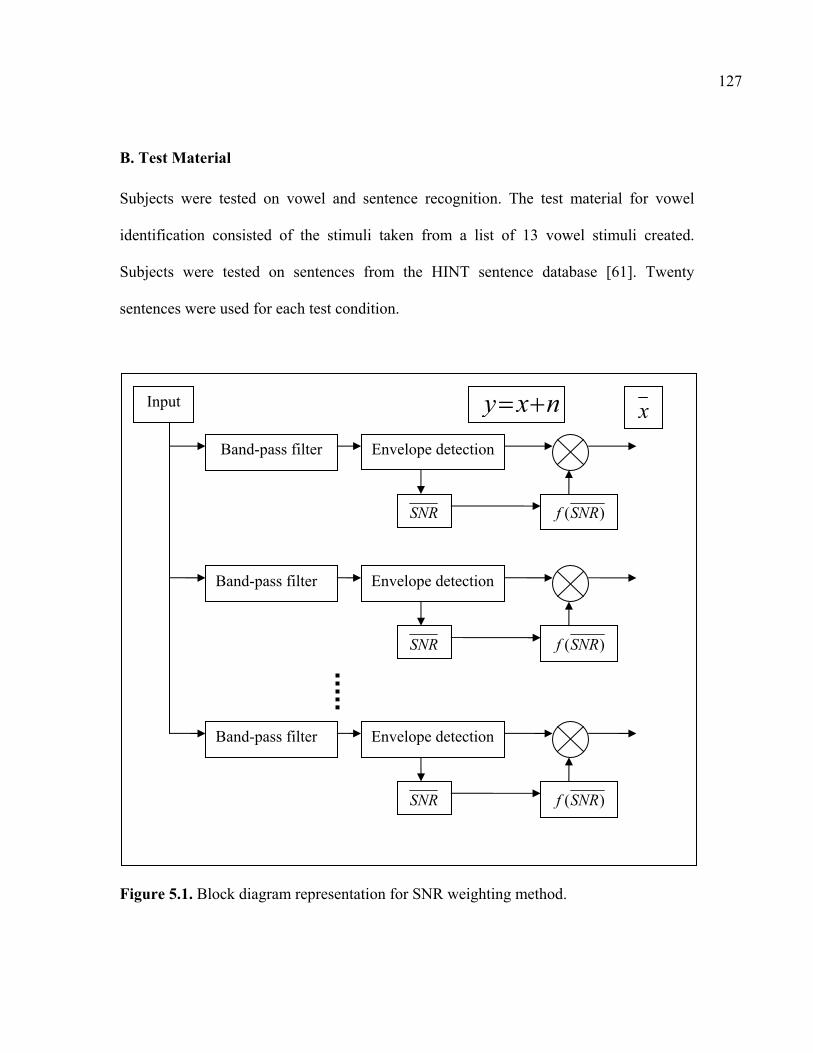
127
B. Test Material
Subjects were tested on vowel and sentence recognition. The test material for vowel
identification consisted of the stimuli taken from a list of 13 vowel stimuli created.
Subjects were tested on sentences from the HINT sentence database [61]. Twenty
sentences were used for each test condition.
Figure 5.1. Block diagram representation for SNR weighting method.
Band-pass filter
Band-pass filter
Envelope detection
Envelope detection
Band-pass filter Envelope detection
SNR
Input
)(SNRf
SNR )(SNRf
SNR )(SNRf
nxy += x

128
Table 5.1. The biographical data for the eight cochlear implant users who were the subjects for the experiments with SNR weighting method. Subject Gender Age at the
time of
testing
Years of
experience
using the
cochlear
implant
Percentage
sentence
recognition
in quiet
Probable
cause of
hearing loss
S1 Male 69 4 88 Unknown
S2 Female 49 4 96 Otosclerosis
S3 Female 52 3 93 Unknown
S4 Female 36 6 96 Unknown
S5 Female 59 3 87 Prescription
drugs
S6 Male 41 3 90 Prenatal
Rubella
S7 Female 46 4 90 Unknown
S8 Female 38 4 87 Genetics
(adolescent
onset loss)
C. Signal Processing
For vowel recognition tests in presence of noise, vowel stimuli were corrupted by speech-
shaped noise at 0 dB and -5 dB SNR levels. For sentence recognition tests in presence of

129
noise, sentence material was corrupted by speech-shaped noise at 10 dB, 5 dB and 0 dB
SNR levels. The noisy input signal was passed through a band-pass filter bank using
sixteen sixth-order Butterworth filters corresponding to the sixteen stimulation electrodes.
The filters were designed to span the frequency range from 350-5500 Hz in a logarithmic
fashion. All the filters were band-pass in nature except the last filter which was high-pass
in nature. The filter edges for the sixteen filters are depicted in Table 4.11. The channel
envelopes were extracted using a rectifier followed by a low-pass filter with 200 Hz cut-
off frequency. The instantaneous SNR was computed by taking the ratio of the
instantaneous signal power and estimated noise power.
The SNR estimation was performed on a sample by sample basis using a decision
directed approach in a way similar to that as done by Ephraim and Malah [13]. The
instantaneous SNR estimate iSNR corresponding to the time instant ‘ i ’ is given by the
following equation:
)0,1max()1(1 −⋅−+⋅= − iii GSNRSNR αα (5.1)
where 22 / iii nyG = , )10( << αα is a smoothing constant, yi is the envelope of noisy
signal in the ith channel and ni is the noise envelope in the ith channel.
The exponential weighting function was generated using the instantaneous SNR
estimate based on the following equation:
)/(exp)( iSNRiSNRf β−= (5.2)
A value of 2=β was used to generate the weighting function.
The resulting gain function using the SNR weighting method is depicted in Figure 5.2.
The gain function using the Wiener filter is also depicted for comparison.

130
Figure 5.2. A plot of the exponential weighting function depicting the gain as a function of SNR. The Wiener gain function is also shown for comparison.
The enhanced signal ix was obtained by multiplying the noisy signal iy by the
exponential weighting function )( iSNRf as given below:
iii ySNRfx ⋅= )( (5.3)
The enhanced signals in each channel were subjected to power law compression
with an exponent value of -0.0001. The compression was tailored to each subject so that
-15 -10 -5 0 5 10 15 20 25 300
0.1
0.2
0.3
0.4
0.5
0.6
0.7
0.8
0.9
1
SNR (dB)
Gai
n Wiener gain function SNR weighting function

131
the compressed output would fall with in the threshold (THR) and the most comfortable
loudness level (MCL) values of the particular cochlear implant user. The electrical
stimulation was presented to the cochlear implant users using the continuous interleaved
sampling strategy (CIS) at a pulse rate determined by the patient’s daily usage settings.
It is worth mentioning that the noise reduction is performed in each channel and is
embedded into the existing CIS strategy. This strategy provides more control over the
noise reduction mechanism since we can perform noise reduction independently on
individual channel outputs and hence provides more flexibility and robustness than the
pre-processing noise reduction methods. The SNR weighting noise reduction is also
attractive in terms of the computational complexity over the pre-processing methods. The
SNR weighting method does not require the use of the Fast Fourier Transform and
complex mathematical calculations and can be readily implemented on the current
cochlear implant processors.
D. Procedure
The cochlear implant subjects were tested on vowel and sentence recognition using the
Clarion research interface-II (Advanced Bionics). For the vowel recognition experiments
the names of the vowels were displayed on a computer monitor and a graphical user
interface enabled the subjects to indicate their response. The subjects were tested in
blocks of 3 repetitions each on the 13 vowel stimuli. The SNR for a particular subject
was chosen based on the vowel recognition score in presence of noise using the baseline
CIS strategy. For the pilot test the SNR was varied across different values (5 dB, 0 dB
and -5 dB) and a SNR value was chosen at which the vowel recognition score dropped

132
very significantly from the vowel recognition score in quiet. One subject S3 was tested
on vowel recognition at 5 dB SNR. Three subjects S1, S6 and S7 were tested on vowel
recognition at 0 dB SNR. Four subjects S2, S4, S5 and S8 were tested on vowel
recognition at -5 dB SNR.
In the case of sentence recognition the subjects were instructed to write down the
words they heard. For each condition the subjects were tested on a list of 20 sentences.
The subjects were allowed to repeat each stimulus one time if needed. The order of the
various test conditions was partially counterbalanced among the various subjects. As in
the vowel recognition test, the subjects were tested on sentence recognition in noise at a
SNR value at which the sentence recognition score dropped very significantly compared
to the sentence recognition score in quiet using the baseline CIS strategy. Two subjects
S2 and S3 were tested on sentence recognition at 10 dB SNR. Three subjects S5, S6 and
S7 were tested on sentence recognition at 5 dB SNR. Three subjects S4 and S8 were
tested on sentence recognition at 0 dB SNR.
5.2.2 Results and discussion
The mean vowel recognition scores in speech-shaped noise with the regular CIS and the
SNR weighting method are depicted in Figure 5.3. The standard errors of mean bars are
shown along with the mean recognition scores. The vowel recognition scores in presence
of speech-shaped noise were significantly higher using the SNR weighting strategy
(SNRW) than regular CIS processing (NCIS). The mean vowel recognition score with the
regular CIS in presence of noise was 42.76%. The mean vowel recognition score with the
SNR weighting noise reduction method was 73.04%.

133
Figure 5.3. Mean vowel recognition in presence of speech-shaped noise using SNR weighting method.
Figure 5.4. Individual subject scores for vowel recognition in presence of speech-shaped noise using SNR weighting method.
0 10 20 30 40 50 60 70 80 90
100
NCIS SNRW
Conditions
Perc
ent c
orre
ct
0 10 20 30 40 50 60 70 80 90
100
S1 S2 S3 S4 S5 S6 S7 S8Subjects
Perc
ent c
orre
ct
NCIS
SNRW

134
Statistical analysis using the paired samples t-test showed that vowel recognition
using the SNR weighting noise reduction method was significantly higher than the CIS
method (p<0.01). The individual subject scores are shown in Figure 5.4. Vowel
perception scores for the three subjects S2, S3 and S7 improved by about 40% with the
SNR weighting noise reduction method (SNRW) compared to the regular CIS processing
(NCIS).
The mean sentence recognition scores with the SNR weighting method and the
CIS are shown in Figure 5.5. The mean sentence recognition score in presence of speech-
shaped noise with the regular CIS method was 65.57%. The mean sentence recognition
score with the SNR weighting noise reduction method was 76.23% higher than the
regular CIS. Statistical analysis using the paired samples t-test showed that the difference
in sentence recognition scores was not statistically significant (p=0.151).
Figure 5.5. Mean sentence recognition in presence of speech-shaped noise using SNR weighting method.
0
10 20 30 40 50 60 70 80 90
100
NCIS SNRW Conditions
Perc
ent c
orre
ct
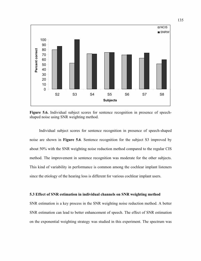
135
Figure 5.6. Individual subject scores for sentence recognition in presence of speech-shaped noise using SNR weighting method.
Individual subject scores for sentence recognition in presence of speech-shaped
noise are shown in Figure 5.6. Sentence recognition for the subject S3 improved by
about 50% with the SNR weighting noise reduction method compared to the regular CIS
method. The improvement in sentence recognition was moderate for the other subjects.
This kind of variability in performance is common among the cochlear implant listeners
since the etiology of the hearing loss is different for various cochlear implant users.
5.3 Effect of SNR estimation in individual channels on SNR weighting method
SNR estimation is a key process in the SNR weighting noise reduction method. A better
SNR estimation can lead to better enhancement of speech. The effect of SNR estimation
on the exponential weighting strategy was studied in this experiment. The spectrum was
0 10 20 30 40 50 60 70 80 90
100
S2 S3 S4 S5 S6 S7 S8Subjects
Perc
ent c
orre
ct
NCISSNRW

136
divided into three different regions namely low-frequency (LF) region, mid-frequency
(MF) region and high-frequency (HF) region.
Noise reduction was performed by varying the SNR estimation between the
decision-directed method and the computed true SNR (computed from the actual speech
and the corrupting noise signals) in the various frequency regions in a systematic manner.
Sentence recognition in the presence of noise was assessed using the SNR weighting
noise reduction algorithm using various SNR estimation methods. Sentence recognition
in noise was evaluated using multi-talker babble noise at 10 dB SNR (Hu et al. [39]).
5.3.1 Experimental Method
A. Subjects
Five cochlear implant users who were recipients of Clarion CII (Advanced Bionics)
processor participated in this experiment. All the subjects were postlingually deafened
adults who used the cochlear implant for a minimum of 2 to 3 years. The biographical
data for the five subjects is presented in Table 5.2.
B. Test Material
The test material consisted of lists of sentences taken from the IEEE database [40]. Lists
of twenty sentences were used for each test condition.
C. Signal Processing
The methodology for signal processing was the same as that described in the Experiment
5.2 except for the method of estimating the SNR. The contribution of SNR estimation in

137
individual channels was evaluated by dividing the frequency spectrum into three regions
(i) low-frequency (LF) region (<1 kHz), (ii) mid-frequency (MF) region (1-3 kHz) and
(iii) high-frequency (HF) region (> 3 kHz). The SNR calculation was performed using the
true SNR estimate in the various frequency regions. The true SNR estimate was
calculated using the clean speech signals and the true additive noise signals from the
speech database used for the experiment.
Table 5.2. The biographical data for the five cochlear implant users who were the subjects for the experiments with SNR estimation in individual channels. Subject Gender Age at the
time of
testing
Years of
experience
using the
cochlear
implant
Percentage
sentence
recognition
in quiet
Probable
cause of
hearing loss
S1 Male 69 4 88 Unknown
S2 Female 36 6 96 Unknown
S3 Female 59 3 87 Prescription
drugs
S4 Female 46 4 90 Unknown
S5 Female 58 4 59 Unknown
Noise reduction was performed in four different ways by varying the SNR
estimation method between the decision directed approach and the true SNR estimation
method in the various frequency regions. Three different noise reduction methods in

138
which the true SNR estimation was used in either low-frequency (LF) region or mid-
frequency (MF) region or high-frequency (HF) region and the decision directed SNR
estimation method was used in the remaining frequency regions. The three noise
reduction methods are denoted as LF method, MF method and HF method respectively.
In the fourth method the noise reduction was performed using the true SNR estimation
method in all the frequency regions and is denoted as ALLF method. For example, in the
LF condition, true SNR estimate was used in the frequency channels falling in low-
frequency region and decision-directed method (DD) for SNR estimation was used the
remaining frequency channels falling into other frequency regions to perform the SNR
weighting noise reduction as described earlier. Sentence recognition in noise was
evaluated for multi-talker babble noise at 10 dB SNR.
D. Procedure
The experimental procedure was the same as that described in Experiment 5.2 for the
sentence recognition tests.
5.3.2 Results and Discussion
The effect of SNR estimation in individual frequency (LF/MF/HF) regions on the SNR
weighting noise reduction method is depicted in Figure 5.7 for the case of multi-talker
babble noise at 10 dB SNR. The standard errors of mean bars are shown along with the
mean recognition scores. Better SNR estimation lead to better sentence recognition as
presented in the ALLF condition. Sentence recognition with the ALLF method improved
by 20.59% compared to the regular CIS method (NCIS).

139
Figure 5.7. Effect of SNR estimation in individual channels for the case of multi-talker babble noise at 10 dB SNR.
The statistical analysis using Tukey test showed that the increase in sentence
recognition with the ALLF method over the regular CIS method was significantly higher
(p<0.05). The improvement in sentence recognition with the LF condition was 24.91%
compared to the regular CIS method. The statistical analysis as per the Tukey test
indicated that the increase in sentence recognition with the LF method over the regular
CIS method was significantly higher (p<0.05). The sentence recognition using the MF,
HF and DD methods were not significantly higher than the regular CIS method (p>0.05).
These results indicate that using a better noise estimate can lead to an improvement in the
sentence recognition using the SNR weighting method as given by the ALLF method.
Another interesting result is that better noise estimate just in the low frequency region as
given by the LF method can lead to significant improvement in sentence recognition.
0 10 20 30 40 50 60 70 80 90
100
CIS NCIS ALLF LF MF HF DD
Conditions
Perc
ent c
orre
ct

140
These results carry important implications for performing noise reduction in the
case of cafeteria noise situation for the cochlear implants. Better noise estimation in low
frequency region alone can lead to improvement in the performance of the noise
reduction method and can significantly reduce the computational complexity of the noise
reduction method.
These results indicate that having access to a relatively “cleaner” signal in either
the mid-frequency region (Formant 2 region) or high frequency region did not provide
significant benefits to speech intelligibility. In contrast, having access to a “cleaner”
signal in the low-frequency region, where Formant 1 (and in some cases Formant 2)
resides, provided significant benefits to speech intelligibility.
The fact that performance improved significantly when the true SNR value was
used in the low frequency channels suggests that multi-talker babble noise must have
masked heavily the low-frequency region of the spectrum. This observation is contrary
to what we know about the effect of multi-talker babble on the spectrum of speech.
Generally, the low-frequency region is masked to a lesser degree than the high-frequency
region due to low-pass nature of the speech spectrum. As a result, normal-hearing
listeners are able to utilize in noisy environments reliable F1 and partial F2 information
for accurate vowel identification and stop-consonant perception (Parikh and Loizou [64]).
The situation with cochlear implant listeners, however, is quite different as they
have a relatively poor frequency resolution in the F1 region and have to rely on
information conveyed by the noise-corrupted envelope. The effect of multi-talker babble
noise on the low-frequency region of the spectrum is thus more detrimental in cochlear
implant listeners than in normal-hearing listeners.

141
We suspect that the benefit introduced in the LF condition was due to a better
representation of F1, and in some cases F2 (e.g., /o/, /u/), information. Hence, in the LF
condition although cochlear implant users might not have a coherent idea on the location
of both F1 and F2 frequencies, they have a good indication about the location of F1 and
only a vague idea about the location of F2. Having a good representation of F1 with
partially vague F2 information can have significantly improve speech perception as
indicated in the studies by Parikh and Loizou [64].
5.4 Novel S-shaped compression techniques for noise suppression
5.4.1 Theoretical derivation of various S-shaped compression curves
A new class of compression techniques that utilize the noise estimate to suppress the
background noise were developed. Most of the compression functions used in current
implant devices employ a power-law function [56] as given by the following equation:
BxAy p +⋅= (5.4)
The output of compression function for a value of 0001.0−=p is shown in
Figure 5.8.
Two compression techniques that suppress the noise to a different extent were
developed. The new techniques divide the compression function into different regions
based upon the noise estimate (Kasturi and Loizou [43]).

142
0 500 1000 1500 2000 25000
100
200
300
400
500
600
700
800
900
1000
Input signal
Com
pres
sion
out
put
Regular power-law compression using an exponent p=-0.0001
Noisy signal portion
Noise floor
Figure 5.8. Regular power-law compression using an exponent p=-0.0001.
5.4.1.1 S-shaped compression
In one approach, the input above the noise level was subjected to the regular compression
function given by Equation 5.5. The input below the estimated noise level was subjected
to an expansion function given by Equation 5.6. This is referred to as S-shaped
compression of Type 1.
1111 BxAy p +⋅= 0001.0, 1 −=pwhere (5.5)
2222 BxAy p +⋅= 8.1, 2 =pwhere (5.6)

143
The coefficients 2211 ,, BandABA are given by the following equations:
)1(/)( 11 −−= psizeTableTHRMCLA (5.7)
)( 11 ATHRB −= (5.8)
)1(/)( 22 −−= pnfTHRKneeA (5.9)
)( 22 ATHRB −= (5.10)
111 BnfAKnee p +⋅= (5.11)
0 500 1000 1500 2000 25000
100
200
300
400
500
600
700
800
900
1000
Input signal
Com
pres
sion
out
put
S-shape compression (Type 1) using exponents p1=-0.0001, p2=1.8
Knee point
Regular compression
S-shape compression
Noise floor
Figure 5.9. S-shaped compression (Type 1) using power exponents p1=-0.0001, p2=1.8.

144
In the preceding set of equations, nf is the estimated noise floor and Knee is the
knee point for the compression curve. MCL is the maximum comfortable loudness level,
THR is the threshold level of electric hearing expressed in micro-amperes and sizeTable
is the size of the compression table (sizeTable = 2048, in our study). The resulting
compression function is shown in Figure 5.9. In the figure, both the regular power-law
compression curve and the S-shape compression curve are shown for comparison
purposes. It can be observed that the s-shape compression suppresses the noise portion of
the signal compared to the regular power-law compression. The portion of the S-shape
curve zoomed in around knee point is shown in Figure 5.10.
0 50 100 150 200 250 300
0
100
200
300
400
500
600
700
Input signal
Com
pres
sion
out
put
S-shape compression (Type 1) using exponents p1=-0.0001, p2=1.8
Knee point
Regular compression
S-shape compression
Noise floor
Figure 5.10. S-shaped compression (Type 1) using power exponents p1=-0.0001, p2=1.8 (zoomed in around the knee point).

145
In another approach a linear function was used to map the noise portion of the
signal instead of the expansive function. A compression function was used for the input
above the noise level given by Equation 5.12. A linear function was used for the input
below the noise level given by Equation 5.13. The coefficients 2211 ,, BandABA are
given by Equations 5.7-5.11. The resulting compression function is shown in Figure
5.11. The portion of the curve around knee point is shown in Figure 5.12. This is referred
to as S-shaped compression of Type 2.
1111 BxAy p +⋅= 0001.0, 1 −=pwhere (5.12)
2222 BxAy p +⋅= 1, 2 =pwhere (5.13)
0 500 1000 1500 2000 25000
100
200
300
400
500
600
700
800
900
1000
Input signal
Com
pres
sion
out
put
S-shape compression (Type 2) using exponents p1=-0.0001, p2=1
Knee point
Regular compression
S-shape compression
Noise floor
Figure 5.11. S-shaped compression (Type 2) using power exponents p1=-0.0001, p2=1.

146
Figure 5.12. S-shaped compression (Type 2) using power exponents p1=-0.0001, p2=1(zoomed in around the knee point).
5.4.2 Evaluation of S-shaped compression techniques for noise reduction in
cochlear implants
5.4.2.1 Experimental Method A. Subjects
Eight cochlear implant users who were recipients of Clarion CII (Advanced Bionics)
processor participated in this experiment. All the subjects were postlingually deafened
adults who used the cochlear implant for a minimum of 2 to 3 years. The biographical
data for the eight subjects is presented in Table 5.3.
0 50 100 150 200 250 0
100
200
300
400
500
600
700
Input signal
Com
pres
sion
out
put
S-shape compression (Type 2) using exponents p1=-0.0001, p2=1
Knee point
Regular compression
S-shape compression
Noise floor

147
Table 5.3. The biographical data for the eight cochlear implant users who participated in the experiments with S-shape compression. Subject Gender Age at the
time of
testing
Years of
experience
using the
cochlear
implant
Percentage
sentence
recognition
in quiet
Probable
cause of
hearing loss
S1 Female 49 4 96 Otosclerosis
S2 Female 36 6 96 Unknown
S3 Female 59 3 87 Prescription
drugs
S4 Female 52 3 93 Unknown
S5 Female 61 3 90 Prescription
drugs
S6 Female 46 4 90 Unknown
S7 Male 69 4 88 Unknown
S8 Female 38 4 87 Genetics
(adolescent
onset loss)
B. Test Material
The sentence material consisted of several lists of phonetically-balanced IEEE sentences
[40]. Subjects were tested on twenty sentences per test condition. Sentence recognition
was tested in presence of speech-shaped noise at 5 dB SNR and multi-talker babble noise

148
at 10 dB and 5 dB SNR levels. Speech-shaped noise used in these experiments was taken
from the HINT database (Nilsson et al. [61]) and multi-talker babble noise composed of
utterances of 10 male and 10 female talkers was taken from the Auditec CD (St. Louis,
MO).
C. Signal Processing
Speech material was first band-pass filtered into 16 logarithmically-spaced frequency
bands using sixth-order Butterworth filters. The filters were designed to span the
frequency range from 350 to 5500 Hz in a logarithmic fashion. All the filters were band-
pass, except for the last filter which was high-pass. The filter edges for the sixteen filters
are depicted in Table 4.11. The output of each channel was passed through a full-wave
rectifier followed by a second order Butterworth low-pass filter with a center frequency
of 200 Hz to obtain the envelope of each channel.
The channel envelope amplitudes were finally compressed according to the
power-law compression and the various S-shaped compression functions as described in
the following section. Electrical pulses whose amplitudes were determined by the
compressed signals were delivered to the electrodes using the continuous interleaved
sampling (CIS) strategy. Electrical pulses were delivered at a rate determined based on
the pulse width used in the subject’s daily processor.
The S-shaped compression mapping of acoustic amplitudes to electrical
amplitudes involved two steps. The first step estimated the noise floor level using a
noise-estimation algorithm. Note that unlike voice-activity detection algorithms, noise
estimation algorithms track the noise continuously, even during speech-active segments.

149
The second step constructed the S-shaped mapping function based on the noise-floor
level estimated in the first step.
(i) Noise estimation method
The first step in the implementation of the proposed S-shaped compression function
involved the estimation of the noise envelope. Since the characteristics of speech-shaped
noise and multi-talker babble noise differ, we used two different methods for estimating
the noise envelope. For the case of speech-shaped noise, which is stationary, the noise
envelope was computed using the initial 120 msecs of speech-absent portion of the
corrupted speech signal. More specifically, the noise envelopes in each channel were
computed by averaging, over the initial 120 msecs segment, the envelopes extracted via
band-pass filtering and full-wave rectification. Since speech-shaped noise is stationary in
nature, the same noise envelope amplitudes were used for all subsequent segments.
A different method was used for tracking the noise envelope of multi-talker
babble and was adapted from Rangachari and Loizou [69]. The noise estimation
algorithm tracks and updates the noise envelope continuously in each speech frame
taking into account the highly non-stationary nature of multi-talker babble noise.
Let the speech corrupted by noise be represented as )()()( tntxty += where
)(tx is the clean speech and )(tn is the noise. The smoothed estimate of the spectrum of
corrupted signal in each channel is computed as given below:
2),()1(),1(),( kYkPkP ληληλ −+−= (5.14)
where ),( kP λ is the smoothed spectrum, λ is the time index and k is the channel index.

150
The local minimum of the corrupted speech signal is computed as follows:
( )
),(),(
),1(),(11),1(),(
),(),1(
min
minmin
min
kPkPotherwise
kPkPkPkP
thenkPkPIf
λλ
λβλβγλγλ
λλ
=
−−−−
+−=
<−
(5.15)
where ),(min kP λ is the local minimum of the corrupted speech and γβ , are experimental
constants.
The ratio of the noisy spectrum and its local minimum is computed as follows:
),(),(),(
min kPkPkSr λ
λλ = (5.16)
If the above ratio is less than a preset threshold, the speech frame is considered to be
speech absent otherwise it is considered to contain speech.
absentspeechkIotherwise
presentspeechkIthenkSIf r
0),(
1),(),(
=
=>
λ
λδλ
(5.17)
where δ is preset threshold.
The speech presence probability is updated according to the following equation:
),()1(),1(),( kIkPkP pp λαλαλ −+−= (5.18)
In the above equation pα is the smoothing factor. Finally the time-frequency dependent
weighting factor is computed as:
),()1(),( kPk dds λααλα −+= (5.19)

151
The value of dα is in the range .1),( ≤≤ ksd λαα The noise spectrum is updated in time
according to the following equation:
2),()),(1(),1(ˆ),(),(ˆ kYkkNkkN ss λλαλλαλ −+−= (5.20)
The following smoothing constants and parameters were used in the implementation of
the noise estimation:
125.0,998.0,8.0,5.0,5.0 ====== δβγααη anddp .
Figure 5.13 shows an example of noise envelope estimation for a sentence
corrupted by multi-talker babble noise at 10 dB SNR.
Figure 5.13. Envelope of noise and the noise envelope estimated using the algorithm.
0 0.5 1 1.5 2 0
200
400
600
Com
pres
sed
outp
ut
0 0.5 1 1.5 2 0
200
400
600
Time (secs)

152
Bottom panel shows the envelopes (thin lines) of noise (multi-talker babble noise
at 10 dB SNR) and the estimated noise envelopes (thick lines) obtained using the noise
estimation algorithm. For better clarity, the top panel shows the envelopes of the noise
alone. Only the noise envelope amplitude of channel 3 (centered at 540 Hz) is shown in
this example. As can be seen, the noise estimation algorithm is capable of tracking, for
the most part, sudden changes of the background noise envelope.
Since the noise estimation algorithm tracks the spectral minima, we considered
applying a bias factor (>1) to the estimated noise envelope amplitude in order to
artificially increase the noise floor level. More specifically, if ( , )D kl is the noise
envelope amplitude computed at time l for channel k by the proposed noise estimation
algorithm, then we considered the following biased estimate of the noise envelope:
),(),(ˆ klDbklD ⋅= (5.21)
where b is the bias factor, ( , )D kl is the estimated noise envelope amplitude and ˆ ( , )D kl
is the biased estimate of the noise envelope amplitude. The bias factor is used as a
parameter for controlling the amount of noise suppression applied. In our experiments,
we considered three different values for b: 1, 2 and 2 2b b b= = = . Use of 1b = sets
the noise floor at a low value resulting in a relatively weak suppression of the noise. The
other two values of b ( 2 and 2 2b b= = ) set the noise floor to a relatively higher
value leading to more aggressive suppression of the noise.
Figure 5.14 shows examples of envelopes estimated using the S-shaped mapping
function ( 2 and 2 2b b= = ) and the log mapping function for a sentence corrupted by
multi-talker babble noise at 10 dB SNR. Only the envelope amplitudes of channel 3
(centered at 540 Hz) are shown in this example.

153
Figure 5.14. Speech envelopes estimated with and without using S-shaped compression.
Top panel shows the envelopes computed for an IEEE sentence in quiet. The
conventional logarithmic function was used to map the acoustic to electrical amplitudes.
Bottom two panels show the envelopes (thick lines) extracted using S-shaped
compression function with 2b = (middle panel) and 2 2b = (bottom panel) for the
same IEEE sentence corrupted by multi-talker babble noise at 10 dB SNR. The
envelopes (thin lines) extracted using the log mapping function are overlaid for
comparative purposes.
It is clear that noise affected for the most part the envelope valleys, with little
effect on the envelope peaks. S-shaped mapping functions suppressed the noise in the
0 0.1 0.2 0.3 0.4 0.5 0.6 0.7 0.8 0.9 1.00
500
1000
0 0.1 0.2 0.3 0.4 0.5 0.6 0.7 0.8 0.9 1.00
500
1000
Com
pres
sed
outp
ut
0 0.1 0.2 0.3 0.4 0.5 0.6 0.7 0.8 0.9 1.00
500
1000
Time (secs)
b=2.0
b=2.8

154
valleys while preserving the peaks. Stronger noise suppression was achieved with
2 2b = than with 2b = . Also, compared to the envelopes obtained with the log
mapping function, a better temporal envelope contrast was achieved with S-shaped
mapping functions.
(ii) Construction of S-shaped mapping function
The estimated noise envelope amplitude ˆ ( , )D kl was subsequently used to construct S-
shaped mapping functions. The knee-point of S-shaped function was computed using the
estimated noise envelope amplitude by setting ),(ˆ klDnf = in Equations 5.7 – 5.11 used
to perform S-shaped compression. Two different compression strategies based on S-
shaped compression (Type 1) and S-shaped compression (Type 2) as described in Section
5.4.1 were developed. S-shaped compression (Type 1) using power exponents p1=-
0.0001, p2=1 is denoted as ‘Type 1’ strategy. S-shaped compression (Type 2) using
power exponents p1=-0.0001, p2=1.8 is denoted as ‘Type 2’ strategy.
D. Procedure
The cochlear implant subjects were tested on sentence recognition with the Clarion
research interface-II (Advanced Bionics). A practice session with ten sentences presented
in quiet was used in the beginning. The practice session lasted for about 5-10 minutes.
After the practice session, the subjects were tested on the various conditions
incorporating the different S-shaped compression functions. Speech-shaped noise was
added to the IEEE sentences at 5 dB SNR, and multi-talker babble noise was added to the
sentences at 5 dB and 10 dB SNR levels. The Type 1 strategy was run using the three
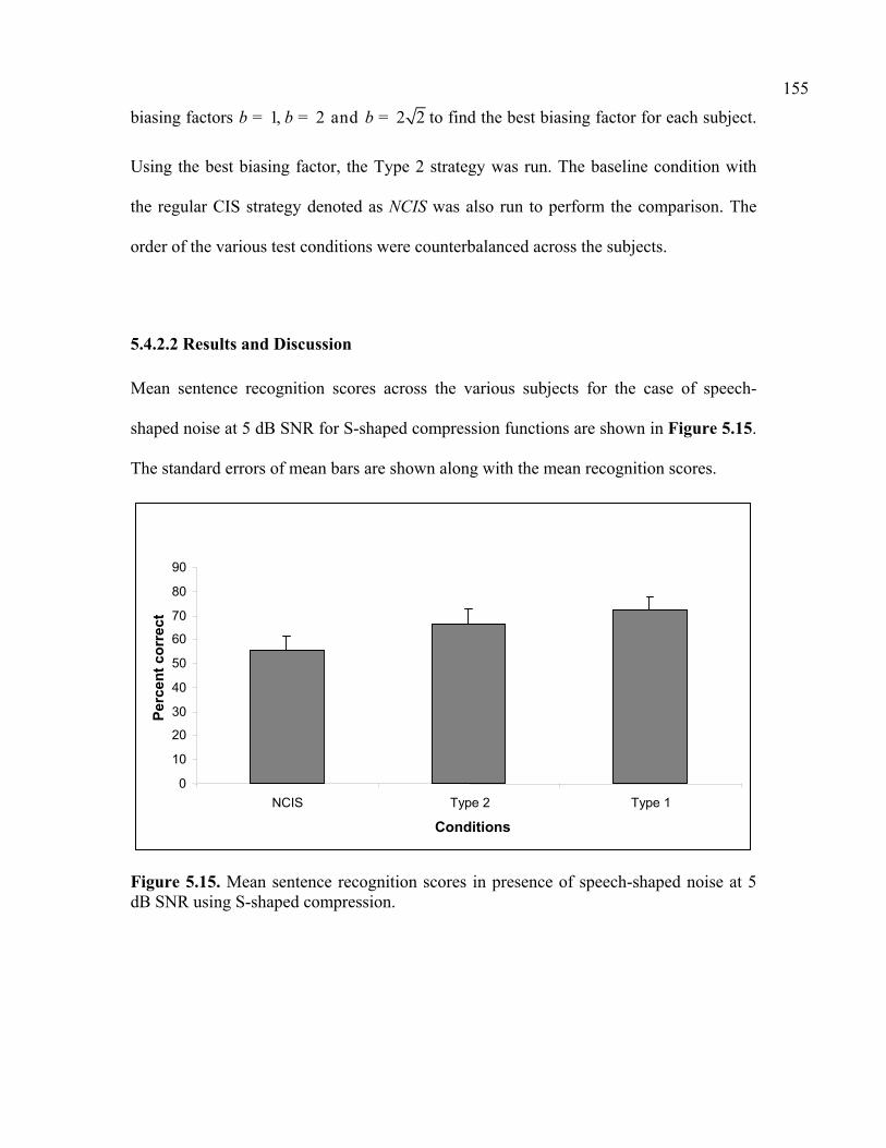
155
biasing factors 1, 2 and 2 2b b b= = = to find the best biasing factor for each subject.
Using the best biasing factor, the Type 2 strategy was run. The baseline condition with
the regular CIS strategy denoted as NCIS was also run to perform the comparison. The
order of the various test conditions were counterbalanced across the subjects.
5.4.2.2 Results and Discussion
Mean sentence recognition scores across the various subjects for the case of speech-
shaped noise at 5 dB SNR for S-shaped compression functions are shown in Figure 5.15.
The standard errors of mean bars are shown along with the mean recognition scores.
Figure 5.15. Mean sentence recognition scores in presence of speech-shaped noise at 5 dB SNR using S-shaped compression.
0 10 20 30 40 50 60 70 80 90
NCIS Type 2 Type 1 Conditions
Perc
ent c
orre
ct

156
0102030405060708090
100
S1 S2 S3 S4 S5 S6 S7 S8
Subjects
Per
cent
cor
rect
NCISType 2Type 1
Figure 5.16. Individual subject scores for sentence recognition in presence of speech-shaped noise at 5 dB SNR using S-shaped compression.
The mean sentence recognition score using the regular CIS (NCIS) was about
55.69%. The mean sentence recognition using Type 1 S-shaped compression was higher
than the regular CIS at about 72.52%. Statistical analysis using the paired samples t-test
indicated that the difference was statistically significant (p<0.05). The mean sentence
recognition using Type 2 strategy was 66.43%. Statistical analysis revealed that the
performance using Type 2 strategy was better than that with regular CIS strategy
(p<0.05). Individual subject scores are shown in Figure 5.16. Subjects S1, S4 and S8
received improvement in sentence recognition by more than 20% using the S-shaped
compression Type 1 strategy compared to the regular CIS strategy.

157
Figure 5.17. Mean sentence recognition scores in presence of multi-talker babble noise at 10 dB SNR using S-shaped compression.
0102030405060708090
100
S1 S2 S3 S4 S5 S6 S7 S8
Subjects
Perc
ent c
orre
ct
NCISType 2Type 1
Figure 5.18. Individual subject scores for sentence recognition in presence of multi-talker babble noise at 10 dB SNR using S-shaped compression.
The mean sentence recognition scores for S-shaped compression functions are
shown for the case of multi-talker babble noise at 10 dB SNR in Figure 5.17. The
0 10 20 30 40 50 60 70 80 90
NCIS Type 2 Type 1 Conditions
Perc
ent c
orre
ct

158
standard errors of mean bars are shown along with the mean recognition scores. The
mean sentence recognition score with the regular CIS condition (NCIS) was 65.44%. The
mean sentence recognition with Type 1 S-shaped compression was higher than the
regular CIS at 76.05%. Statistical analysis using the paired samples t-test showed that the
difference was statistically significant (p<0.005). The mean sentence recognition score
using S-shaped compression of Type 2 was 68.07%. Statistical analysis revealed that the
performance with Type 2 S-shaped compression was the same as that with the regular
CIS (p=0.558). Individual subject scores are shown in Figure 5.18. Subjects S4 and S7
improved in sentence recognition by about 20% using S-shaped compression of Type 1
strategy compared to the regular CIS strategy.
0
10
20
30
40
50
60
70
80
90
NCIS Type 2 Type 1
Conditions
Perc
ent c
orre
ct
Figure 5.19. Mean sentence recognition scores in presence of multi-talker babble noise at 5 dB SNR using S-shaped compression.

159
0
10
20
30
40
50
60
70
80
S1 S2 S3 S4 S5 S6 S7 S8
Subjects
Per
cent
cor
rect
NCISType 2Type 1
Figure 5.20. Individual subject scores for sentence recognition in presence of multi-talker babble noise at 5 dB SNR using S-shaped compression.
For the case of multi-talker babble noise at 5 dB SNR the results for S-shaped
mapping functions are in Figure 5.19. The standard errors of mean bars are shown along
with the mean recognition scores. The mean sentence recognition score with the regular
CIS (NCIS) condition was 30.03%. The mean sentence recognition with Type 1 S-shaped
compression was higher at 39.98%. Statistical analysis using the paired samples t-test
revealed that the difference was statistically significant (p<0.05). The mean sentence
recognition score using the Type 2 strategy was 35.16%. Statistical analysis using the
paired samples t-test showed that the difference was not statistically significant (p=0.21).
Individual subject scores are shown in Figure 5.20. Subjects S2, S3, S5 and S8 improved
in sentence recognition by about 15% with S-shaped compression Type 1 compared to
the regular CIS condition.
These results demonstrated that the shape of the non-linear acoustic-to-electric
mapping function can have a significant effect on speech perception in noise. The log
160
functions currently used in most implant processors for mapping acoustic to electric
amplitudes are not the best mapping functions for noisy environments. This is largely
because compressive functions tend to amplify low-level segments of speech along with
noise, thereby decreasing the spectral contrast and effective dynamic range. In contrast,
S-shaped mapping functions, which are partly compressive and partly expansive
depending on the signal level, are more suitable for noisy environments and can produce
significantly better performance than the log-mapping functions.
One factor has possibly contributed to the benefit of S-shaped mapping functions
and that is improved spectral contrast. As can be seen in Figure 5.14, S-shaped
compression preserves the envelope peaks and deepens the valleys, which are otherwise
filled for the most part with noise. Furthermore, S-shaped functions improve spectral
contrast without compromising loudness. Use of linear mapping functions generally
improves spectral contrast, but at the expense of reducing significantly the loudness of
the acoustic stimuli thereby rendering most speech segments inaudible or not sufficiently
loud. Several studies (e.g., Fu and Shannon [19]) have confirmed that any dramatic
deviation from a power-law (log type) compressive function will deteriorate
performance. S-shaped functions maintain the log mapping function for input levels
above the estimated noise floor (knee-point). As such, it preserves the loudness of signals
falling above the noise floor while reducing the loudness of signals falling below the
knee-point and possibly dominated by noise.
S-shaped functions suppress the signal falling below the knee-point assumed to
contain primarily noise. It is reasonable to ask why suppress and not annihilate (e.g., zero
out) any signal falling below the knee point. One would expect that that would provide

161
better suppression of the noise. We do not believe that is true for two main reasons. First,
eliminating the signal falling below the knee-point (noise floor) would be a reasonable,
and perhaps a better, approach provided that we are somehow capable of estimating the
noise level (knee point) very accurately. That is not the case in practice, as the noise level
constantly changes, and the best we can do is to estimate, at least conservatively, the
noise floor level. Any errors in over-estimating the noise floor level would wipe out
segments of speech containing useful information thereby degrading intelligibility.
Second, the frequent switching from signal-on to signal-off across and within each
channel would produce undesirable distortion effects. Hence, suppressing rather than
zeroing out the signal falling below the knee point seems to be a safer approach.
We expect larger improvements in performance of S-shaped compression
functions with more accurate estimates of the noise floor, and therefore better estimates
of the knee point. Further research is therefore needed to improve the accuracy and
adaptation time of noise tracking algorithms.

162
CHAPTER 6
CONCLUSIONS This dissertation assessed the effect of various parameters on melody recognition in the
context of cochlear implants in a systematic manner using cochlear implant simulation
experiments with normal hearing listeners. A significant effect of filter spacing employed
for synthesis on melody recognition was observed. The frequency placement of the filters
rather than the number of filters employed was found to be important for melody
recognition. Using just four optimally placed filters as given by the ‘Semitone filter
spacing’ nearly asymptotic performance in melody recognition was obtained. Frequency
up-shifting is an inherent problem with cochlear implants due to variable electrode
insertion depths. Experiments with frequency transposed melodies indicated that the
semitone filter spacing is not significantly affected by frequency up-shifting.
Cochlear implant simulation experiments also showed a significant effect of the
relative phase on melody recognition. Using optimal phase estimation nearly asymptotic
performance with mean melody recognition score of around 100% was obtained with just
three frequency channels. Mean melody recognition score was less than 40% even with
32 frequency channels, when no phase information was used. When the phase
information was systematically corrupted by increasing the random phase jitter, melody
recognition dropped from nearly perfect recognition (about 100%) to chance level
recognition (around 10%). Thus the fine structure information is very important for

163
melody recognition and needs to be coded in a better way in the future cochlear implant
processors.
Melody recognition experiments with cochlear implant patients showed that
melody recognition using just 6 semitone-spaced filter bands was better than that with
sixteen conventional logarithmic filter bands for some cochlear implant users. Preference
tests showed that the semitone filter spacing using just 6 filter bands was highly preferred
(as sounding more melodious) over the conventional logarithmic filter spacing using 16
filter bands with mean preference score of more than 95%. These results indicate that the
semitone filter spacing is a viable candidate for use with cochlear implants to improve
melody recognition.
Most of the noise reduction methods developed for cochlear implants are pre-
processing methods. In this dissertation we investigated the use of two noise reduction
methods namely the ‘SNR weighting method’ and the ‘S-shaped compression’, which are
embedded into the existing cochlear implant signal processing methodology. The
advantages of these embedded noise reduction methods include reduced computational
complexity, ease of implementation and better control of the noise reduction mechanism.
Experiments with cochlear implant patients showed that the mean vowel recognition in
presence of speech-shaped noise improved from nearly 40% using their daily strategy to
about 70% using the SNR weighting method. Thus the SNR weighting method produced
significant improvement in vowel recognition in presence of noise over the CIS strategy
used daily by the cochlear implant patients.
Experiments with SNR estimation in individual frequency regions showed that
better noise estimation can lead to significant improvement in sentence recognition as

164
well, using the SNR weighting method. Better noise estimation in the low frequency
region (<1 kHz) alone can significantly improve the performance of the SNR weighting
method. These results indicate that better noise estimation methods are needed to further
improve speech perception with cochlear implants in noisy listening conditions.
Experiments with cochlear implant patients showed that the S-shaped compression
of Type 2 yielded sentence recognition scores that were significantly higher than that
obtained by using the CIS strategy for the case of speech-shaped noise. Results indicated
that sentence recognition with the S-shaped compression of Type 1 was significantly
better than that with the CIS strategy for both speech-shaped noise and multi-talker
babble noise. Thus, using an expansive function for the noisy portion yielded better
suppression of noise than using a linear function. Sentence recognition using the S-
shaped compression of Type 1 was significantly higher than that obtained using the CIS
strategy for very high noise levels, as in the case of 5 dB speech-shaped noise and 5 dB
multi-talker babble noise. This increase in speech perception can be attributed to the
improvement of spectral contrast by the S-shaped compression of Type 1.
6.1 Major Contributions of this dissertation
In this dissertation, we proposed a novel filter spacing technique for melody
recognition, namely the ‘Semitone filter spacing’ in which filter bandwidths are
varied in correspondence to semitone steps based on melodic center of gravity.
The method is designed to enhance spectral cues and improve melody recognition
with cochlear implants.
Developed the SNR weighting method which is embedded into the CIS strategy.
The advantages of this embedded noise reduction method are reduced

165
computational complexity, ease of implementation and better control of the noise
reduction mechanism.
Developed the S-shaped compression method that divides the compression curve
into two regions based on the computed noise estimate. This is also an embedded
noise reduction method and uses different compression functions for the noise
portion and the speech portion of the signal to better suppress the noise.
6.2 Future Work
The semitone filter spacing proposed in this dissertation can be used to improve
recognition of melodies with the note frequencies falling in different frequency
regions. This can be accomplished by performing the fundamental frequency (F0)
detection and using the semitone filter spacing in that frequency range.
Results from the phase experiments performed in this dissertation indicate that
fine structure information needs to be better coded into the future cochlear
implants to improve melody recognition.
Future work is also needed to obtain better noise estimates in highly noisy
environments to improve the performance of noise reduction methods for cochlear
implants.

166
REFERENCES
[1] Bacon, S. P., Fay, R. R. and Popper, A. N., “Compression: From cochlea to cochlear implants,” Springer-Verlag, New York, 2004.
[2] Baer, T., Moore, B. C. J. and Gatehouse, S., “Spectral contrast enhancement of speech in noise for listeners with sensorineural hearing impairment: Effects on intelligibility, quality and response times,” J. Rehab. Res. Dev., vol. 30, no. 1, pp. 49-72, 1993.
[3] Bassim, M. K., Buss, E., Clark, M. S., Kolln, K. A., Pillsbury, C. H., Pillsbury, H. C. and Buchman, C. A., “MED-EL Combi40+ cochlear implantation in adults,” Laryngoscope, vol. 115, pp. 1568-1573, 2005.
[4] Berouti, M., Schwartz, R. and Makhoul, J., “Enhancement of speech corrupted by acoustic noise,” Proc. Int. Conf. Acoust., Speech, Signal Process., pp. 208-211, 1979.
[5] Boothroyd, A., Hanin, L. and Hnath, T., “A sentence test of speech perception: Reliability, set equivalence and short-term learning,” New York: City University of New York, Internal Report RCI 10, 1985.
[6] Bregman, A. S., “Auditory scene analysis: The perceptual organization of sound,” The MIT Press, Cambridge, 1999.
[7] Clark, G., “Cochlear implants: Fundamentals & Applications,” Springer-Verlag, New York, 2003.
[8] Danhauer, J., Ghadialy, F., Eskwitt, D. and Mendel, L., “Performance of 3M/House cochlear implant users on speech perception,” J. Am. Acad. Audio., vol. 1, pp. 236-239, 1990.

167
[9] de Cheveigne, A., “Cancellation model of pitch perception,” J. Acoust. Soc. Am., vol. 103, no. 3, pp. 1261-1271, 1998.
[10] Dorman, M. F., Hannley, M., Dankowski, K., Smith, L. and McCandless, G., “Word recognition by 50 patients fitted with the Symbion multi-channel cochlear implant,” Ear Hear., vol. 10, pp. 44-49, 1989.
[11] Dorman, M. F., Loizou, P. and Rainey, D “Simulating the effect of cochlear implant insertion depth on speech understanding,” J. Acoust. Soc. Am., vol. 102, no. 5, pp. 2993-2996, 1997.
[12] Eddington, D. K., Rabinowitz, W. R., Tierney, J., Noel. V. and Whearty, M., “Speech processors for auditory prostheses,” NIH contract N01-DC-6-2100, Eight Quarterly Progress Report, 1997.
[13] Ephraim, Y. and Malah, D., “Speech enhancement using a minimum mean-square error short-time spectral amplitude estimator,” IEEE Trans. Acoust., Speech, Signal Process., vol. 32, pp. 1109-1121, 1984.
[14] Ephraim, Y. and Van Trees, H. L., “A signal subspace approach for speech enhancement,” IEEE Trans. Speech and Audio Process., vol. 3, no. 4, pp. 251-266, 1995.
[15] Fetterman, B. and Domico, E., “Speech recognition in background noise of cochlear implant patients,” Otolaryngol. Head Neck Surg., vol. 126, pp. 257-263, 2002.
[16] Filipo, P., Mancini, P., Ballantyne, D., Bosco, E. and D’Elia, C., “Short-term study of the effect of speech coding strategy on the auditory performance of pre- and post-lingually deafened adults implanted with the Clarion CII,” Acta Otolaryngol., vol. 124, pp. 368-370, 2004.
[17] Fishman, K. E., Shannon, R. V. and Slattery, W. H., “Speech recognition as a function of the number of electrodes used in the SPEAK cochlear implant speech processor,” J. Speech Hear. Res., Vol. 40, no. 5, pp. 1201-1215, 1997.

168
[18] Friesen, L., Shannon, R., Baskent, D. and Wang, X., “Speech recognition in noise as a function of the number of spectral channels: Comparison of acoustic hearing and cochlear implants,” J. Acoust. Soc. Am., vol. 110, no. 2, pp. 1150-1163, 2001.
[19] Fu, Q.-J. and Shannon R. V., “Effect of amplitude nonlinearity on phoneme recognition by cochlear implant users and normal-hearing listeners,” J. Acoust. Soc. Am., vol. 104, no. 5, pp. 2570-2577, 1998.
[20] Fu, Q.-J. and Shannon R. V., “Phoneme recognition by cochlear implant users as a function of signal-to-noise ratio and nonlinear amplitude mapping,” J. Acoust. Soc. Am., vol. 106, no. 2, pp. L18-L23, 1999.
[21] Fu, Q.-J. and Shannon R. V., “Recognition of spectrally degraded and frequency-shifted vowels in acoustic and electric hearing,” J. Acoust. Soc. Am., vol. 105, no.3, pp. 1889-1900, 1999.
[22] Fu, Q.-J., Shannon R. V. and Wang, X., “Effects of noise and spectral resolution on vowel and consonant recognition: Acoustic and electric hearing,” J. Acoust. Soc. Am., vol. 104, no.6, pp. 3586-3596, 1998.
[23] Geurts, L. and Wouters, J., “Coding of the fundamental frequency in continuous interleaved sampling processors for cochlear implants,” J. Acoust. Soc. Am., vol. 109, no. 2, pp. 713-726, 2001.
[24] Geurts, L. and Wouters, J., “Better place-coding of the fundamental frequency in cochlear implants,” J. Acoust. Soc. Am., vol. 115, no. 2, pp. 844-852, 2004.
[25] Gfeller, K. and Lansing, C., “Melodic, rhythmic, and timbral perception of adult cochlear implant users,” J. Speech Hear. Res, vol. 34, pp. 916-920, 1991.
[26] Gfeller, K., Olszewski, C., Rychener, M., Sena, K., Witt, S., Knutson, J. F. and Macpherson, B., “Recognition of “real-world” musical excerpts by cochlear implant recipients and normal-hearing adults,” Ear Hear., vol. 26, no. 3, pp. 173-185, 2005.
[27] Glasberg, B. R. and Moore, B. C. J., “Derivation of auditory filter shapes from notch-noised data,” Hear. Res., vol. 47, pp. 103-138, 1990.

169
[28] Gordon, E. E., “Primary measures of music audiation,” G.I.A. Publications, Chicago, 1979.
[29] Gray, R. F., “Cochlear implants,” College-Hill Press, San Diego, 1985.
[30] Green, T., Faulkner, A. and Rosen, S., “Enhancing temporal cues to voice pitch in continuous interleaved sampling cochlear implants,” J. Acoust. Soc. Am., vol. 116, no. 4, pp. 2298-2310, 2004.
[31] Griffiths, L. J. and Jim, C. W., “An alternative approach to linearly constrained adaptive beam forming,” IEEE Trans. Antennas Propag., AP-30, pp. 27-30, 1982.
[32] Hamacher, V., Doering, W., Mauer, G., Fleischmann, H. and Hennecke, J., “Evaluation of noise reduction systems for cochlear implant users in different acoustic environments,” Am. J. Otol., vol. 18, pp. S46-S49, 1997.
[33] Hartmann, W.M., “Pitch, periodicity, and auditory organization,” J. Acoust. Soc. Am., vol. 100, no. 6, pp. 3491-3502, 1996.
[34] Hartmann, W. M. and Johnson, D., “Stream segregation and peripheral channeling,” Music perception, vol. 9, no. 2, pp. 155-184, 1991.
[35] Hillenbrand, J., Getty, L., Clark, M. and Wheeler, K., “Acoustic characteristics of American English vowels,” J. Acoust. Soc. Am., vol. 97, pp. 3099-3111, 1995.
[36] Hollow, R. D., Dowell, R. C., Cowan, R. S. C., Skok, M. C., Pyman, B. C. and Clark, G. M., “Continuing improvements in speech processing for adult cochlear implant patients,” Ann. Otol. Rhinol. Laryngol., Suppl. 166, no. 104, pp. 292-294, 1995.
[37] Houstma, A. J. M. and Smurzynski, J., “Pitch identification and discrimination for complex tones with many harmonics,” J. Acoust. Soc. Am., vol. 87, no. 1, pp. 304-310, 1990.

170
[38] Hu, Y. and Loizou, P., “A generalized subspace approach for enhancing speech corrupted with colored noise,” IEEE Trans. Speech and Audio Process., vol. 11, no. 4, pp. 334-341, 2003.
[39] Hu, Y., Loizou, P., Ning, L. and Kasturi K., “Noise reduction in cochlear implants by SNR weighting,” submitted to J. Acoust. Soc. Am., 2006.
[40] IEEE Subcommittee, “IEEE Recommended Practice for Speech Quality Measurements,” IEEE Trans. Audio and Electroacoustics, AU-17, pp. 225-246, 1969.
[41] Kasturi K. and Loizou, P., “Effect of Filter spacing and correct tonotopic representation on melody recognition: Implications for cochlear implants,’’ Proc. ARO, New Orleans, LA, 2005.
[42] Kasturi K. and Loizou, P., “Filter spacing strategies based on musical semitone scale for better music perception in cochlear implants,” in preparation for J. Acoust. Soc. Am., 2006.
[43] Kasturi K. and Loizou, P., “Use of s-shaped input-output functions for noise suppression in cochlear implants,” submitted to Ear Hear., 2006.
[44] Kay, S. M., “Fundamentals of statistical signal processing: Estimation theory,” Prentice-Hall, New Jersey, 1993.
[45] Kessler, D. K., “The Clarion multi-strategy cochlear implant,” Ann. Otol. Rhinol. Laryngol., Suppl. 177, no. 108, pp. 8-16, 1999.
[46] Kong, Y., Cruz R., Jones J. and Zeng F., “Music perception with temporal cues in acoustic and electric hearing,” Ear Hear., vol. 25, no. 2, pp. 173-185, 2004.
[47] Kong, Y., Vongphoe, M. and Zeng F., “Independent contributions of amplitude and frequency modulations to auditory perception: Melody, tone and speaker identification,” Proc. of ARO., 2003.

171
[48] Laneau, J., Moonen, M. and Wouters, J., “Relative contributions of temporal and place pitch cues to fundamental frequency discrimination in cochlear implantees,” J. Acoust. Soc. Am., vol. 116, no. 6, pp. 3606-3619, 2004.
[49] Levitt, H., “Transformed up-down methods in psychoacoustics,” J. Acoust. Soc. Am., vol. 49, no. 2B, pp. 467-477, 1971.
[50] Lim, J. S. and Oppenheim, A. V., “Enhancement and bandwidth compression of noisy speech,” Proc. of the IEEE., vol. 67, no. 12, pp. 221-239, 1979.
[51] Lockwood, P. and Boudy, J., “Experiments with a nonlinear spectral subtractor (NSS), Hidden Markov Models and the projection, for robust speech recognition in cars,” Speech Communication, vol. 11, pp. 215-228, 1992.
[52] Loeb, G. and Kessler, D., “Speech recognition performance over time with the Clarion cochlear prosthesis,” Ann. Otol. Rhinol. Laryngol., vol. 104, pp. 290-292, 1995.
[53] Loizou, P., “Mimicking the human ear: An overview of signal processing techniques for converting sound to electrical signals in cochlear implants,” IEEE Signal Process. Magazine, vol. 15, no. 5, pp. 101 – 130, 1998.
[54] Loizou, P., “Speech processing in vocoder-centric cochlear implants: in Cochlear and brainstem implants,” Moller, A. R. (ed.), Karger, Basel, pp. 109 – 143, 2006.
[55] Loizou, P., Lobo, A. and Hu, Y., “Subspace algorithms for noise reduction in cochlear implants,” J. Acoust. Soc. Am., vol. 118, no. 5, pp. 2791-2793, 2005.
[56] Loizou, P., Poroy O. and Dorman M., “The effect of parametric variations of cochlear implant processors on speech understanding,” J. Acoust. Soc. Am., vol. 108, pp. 790-802, 2000.
[57] McAulay, R. J. and Malpass, M. L., “Speech enhancement using a soft-decision noise suppression filter,” IEEE Trans. Acoust., Speech, Signal Process., ASSP-28, pp. 137-145, 1980.

172
[58] Meddis, R. and Hewitt, M. J., “Virtual pitch and phase sensitivity of a computer model of the auditory periphery. II: Pitch identification,” J. Acoust. Soc. Am., vol. 89, no. 6, pp. 2866-2882, 1991.
[59] Meddis, R. and Hewitt, M. J., “Virtual pitch and phase sensitivity of a computer model of the auditory periphery. II: Phase sensitivity,” J. Acoust. Soc. Am., vol. 89, no. 6, pp. 2883-2894, 1991.
[60] Moore, B.C.J. and Rosen, S.M., “Tune recognition with reduced pitch and interval information,” J. Exp. Psych., vol. 31, pp. 229-240, 1979.
[61] Nilsson, M., Soli S. and Sullivan J., “Development of Hearing in Noise Test for the measurement of speech reception thresholds in quiet and in noise,” J. Acoust. Soc. Am., vol. 95, pp. 1085-1099, 1994.
[62] Oppenheim, A. V. and Schafer, R. W., “Discrete-time signal processing,” Prentice-Hall, New Jersey, 1989.
[63] Oxenham, A. J., Bernstein, J. G. W. and Penagos, H., “Correct tonotopic representation is necessary for complex pitch perception,” Proc. Nat. Proc. Sc., vol. 101, no. 5, pp. 1421-1425, 2004.
[64] Parikh, G. and Loizou P., “The influence of noise on vowel and consonant cues,” J. Acoust. Soc .Am., vol. 118, no. 6, pp. 3874-3888, 2005.
[65] Patterson, R. D., “Auditory filter shapes derived with noise stimuli,” J. Acoust. Soc. Am., vol. 59, no. 3, pp. 640-654, 1976.
[66] Peeters, S., Offeciers, F. E., Joris, Ph. and Moeneclaey, L., ‘‘The Laura cochlear implant programmed with the continuous interleaved and phase-locked continuous interleaved strategies,’’ Adv. Otol. Rhinol. Laryngol., vol. 48, pp. 261–268, 1993.
[67] Pijl, S. and Schwarz D. W. F., “Melody recognition and musical interval perception by deaf subjects stimulated with electrical pulse trains through single cochlear implant electrodes,” J. Acoust. Soc .Am., vol. 98, no. 2, pp. 886-895, 1995.

173
[68] Poroy, O. and Loizou, P., “Development of a speech processor for laboratory
experiments with cochlear implant patients,” Proc. Int. Conf. Acoust., Speech, Signal Process., 2000.
[69] Rangachari, S. and Loizou P., “A noise estimation algorithm for highly non-stationary environments,” Speech Communication, vol. 28, pp. 220-231, 2006.
[70] Rosen, S., Faulkner, A. and Wilkinson L., “Adaptation by normal listeners to upward spectral shifts of speech: implications for cochlear implants,” J. Acoust. Soc .Am., vol. 106, no. 6, pp. 3629-3636, 1999.
[71] Schulz, E. and Kerber, M., “Music perception with the MED-EL implants,” Advances in Cochlear Implants, pp. 326-332, 1994.
[72] Seligman, P. M. and McDermott, H. J., “Architecture of the SPECTRA 22 speech processor,” Ann. Otol. Rhinol. Laryngol., Suppl. 166, no. 104, pp. 139-141, 1995.
[73] Shannon, R. V., Adams, D. D., Ferrel, R. L., Palumbo, R. L. and Grantgenett M., “A computer interface for psychophysical and speech research with the Nucleus cochlear implant,” J. Acoust. Soc .Am., vol. 87, no. 2, pp. 905-907, 1990.
[74] Shannon, R. V., Jensvold, A., Padilla, M., Robert, M. and Wang, X., “Consonant recordings for speech testing,” J. Acoust. Soc .Am., vol. 106, no. 6, pp. L71-L74, 1999.
[75] Shannon, R. V., Zeng, F., Kamath, V., Wygonski, J. and Ekelid, M., “Speech recognition with primarily temporal cues,” Science, vol. 270, pp. 303-304, 1995.
[76] Silverman, S. R. and Hirsh, I. J., “Problems related to the use of speech in clinical audiometry,” Ann. Otol. Rhinol. Laryngol., vol. 166, no. 64, pp. 1234-1244, 1955.
[77] Smith, Z. M., Delgutte, B. and Oxenham, A. J., “Chimaeric sounds reveal dichotomies in auditory perception,” Nature, vol. 416, pp. 87-90, 2002.

174
[78] Spahr, A. J. and Dorman, M. F., “Performance of subjects fit with the Advanced Bionics CII and Nucleus 3G cochlear implant devices,” Arch. Otolaryngol. Head Neck Surg., vol. 130, pp. 624-628, 2004.
[79] Stevens, S. S. and Volkmann, J., “A scale for the measurement of the psychological magnitude pitch,” J. Acoust. Soc .Am., vol. 8, pp. 185-190, 1937.
[80] Tyler, R., Preece, J. and Lowder, M., “The Iowa audiovisual speech perception laser videodisc. Laser Videodisc and Laboratory Report,” Dept. of Otolaryngology, Head and Neck Surgery, University of Iowa Hospital and Clinics, Iowa City, 1987.
[81] Vandali, A. E., Whitford, L. A., Plant, K. L. and Clark G. M., “Speech perception as a function of electrical stimulation rate: Using the Nucleus 24 cochlear implant system,” Ear Hear., vol. 21, pp. 608-624, 2000.
[82] Van Hoesel, R. and Clark, G., “Evaluation of a portable two-microphone adaptive beamforming speech processor with cochlear implant patients,” J. Acoust. Soc. Am., vol. 97, no. 4, pp. 2498-2503, 1995.
[83] Wilson, B. S., Finley, C. C., Lawson, D. T., Wolford, R. D., Eddington, D. K. and Rabinowitz, W. M., “Better speech recognition with cochlear implants,” Nature, vol. 352, pp. 236-238, 1991.
[84] Wouters, J. and Vanden Berghe J., “Speech recognition in noise for cochlear implantees with a two-microphone monaural adaptive noise reduction system,” Ear Hear. 22, pp. 420-430, 2001.
[85] Yang, L. and Fu, Q., “Spectral subtraction-based speech enhancement for cochlear implant patients in background noise,” J. Acoust. Soc. Am. (L), vol. 117, no. 3, pp. 1001-1004, 2005.

175
[86] Zeng, F.-G. and Galvin, J., “Amplitude mapping and phoneme recognition in cochlear implant listeners,” Ear. Hear., vol. 20, pp. 60-74, 1994.
[87] Zeng, F.-G., Grant, G., Niparko, J., Galvin, J., Shannon, R. V., Opie, J. and Segel, P., “Speech dynamic range and its effect on cochlear implant performance,” J. Acoust. Soc. Am., vol. 111, no. 1, pp. 377-386, 2002.

VITA
Kalyan Kasturi was born in Guntur, India on February 3, 1976, the son of Shri Kasturi V.
M. K. Sarma and Shrimati Amruta Valli. He has two siblings, an elder sister Hema Lata
and a younger brother Mytreya Viswanadh. After completing his pre-university education
from B. V. K. Junior College, Visakhapatnam, he joined the Nagarjuna University,
Vijayawada India, where he received the Bachelors degree in Electronics and
Communications Engineering in 1999.
He was admitted to the Masters program in the Department of Electrical
Engineering at the University of Texas at Dallas in January 2000. He has been working
with the Speech Processing Research Laboratory at the University of Texas at Dallas
since May 2000. He received the Master of Science in Electrical Engineering in August
2002. His master’s thesis was published as an article in the Journal of Acoustical Society
of America. He joined the Doctoral program in the Department of Electrical Engineering
at the University of Texas at Dallas in August 2002. He was a recipient of a Travel award
for Graduate students for the Association for Research in Otolaryngology (ARO)
meeting, 2005. He was a recipient of financial aid scholarship to attend the Conference
on Implantable Auditory Prostheses (CIAP), 2005. Currently he is employed at Texas
Instruments Inc., Dallas.