Novel Decentralized Node Failure RecoveryScheme in Virtualized Networks

by

Habib Abid

Thesis submitted to the

Faculty of Graduate and Postdoctoral Studies

In partial fulfillment of the requirements

For the M.Sc. degree in

Computer Science

School of Computer Science and Electrical Engineering

Faculty of Computer Science

University of Ottawa

c⃝ Habib Abid, Ottawa, Canada, 2013

Abstract

The current Internet infrastructure, managed by multiple stakeholders, is unable to re-

spond to the increasing new demands of services as it is hard to put the conflicted objec-

tives of multiple Internet service providers together. Network virtualization has emerged

as a new paradigm that overcomes the above challenge by partitioning the physical net-

work to multiple isolated virtual networks used by different clients. Network resources

failure is one of the issues that affect the network performance, which in turn impairs

the service offered to the clients.

This thesis addresses the problem of recovering virtual networks (VNs) affected by a

substrate node failure. A novel heuristics-based algorithm that efficiently reallocates

new resources to the affected VNs after a node failure is proposed. In this algorithm, a

manager substrate node executes a set of recovery steps to migrate all the hosted virtual

nodes in the failed substrate node in addition to the virtual paths traveling across it. The

proposed approach is executed in a distributed manner without any coordination from

the central infrastructure provider. The developed scheme efficiently minimizes the node

failure recovery cost, the time needed to recover the virtual nodes hosted on the failed

substrate node and hence significantly reduces the service interruption period. This,

in turn, results in increasing the service provider revenue and decreasing the penalty

charges paid for service level agreement violation. Performance results demonstrate the

significant reduction in VN service cost and interruption time.

ii

Acknowledgements

First and foremost I have to thank Almighty Allah, the Lord of the Worlds, the Merciful,

and the Compassionate, for providing me the determination and energy to complete this

work.

I would like to express my gratitude and appreciation to my supervisor, Professor Nancy

Samaan for her guidance and support during my research. She has been a true mentor

and a major source of support and encouragement, her feedback and input were essential

to reach my goals in this thesis.

Also, many thanks to my wife and children for their patience to be with me along the

way of my study and for providing me the hope to continue my education.

Finally, I would like to thank my mother for the life she gave me, prayer, strength and

pride she offered me.

iii

Contents

1 Introduction 2

1.1 Introduction . . . . . . . . . . . . . . . . . . . . . . . . . . . . . . . . . . 2

1.2 Contribution . . . . . . . . . . . . . . . . . . . . . . . . . . . . . . . . . . 3

1.3 Thesis Structure . . . . . . . . . . . . . . . . . . . . . . . . . . . . . . . . 4

2 Background and Related Work 5

2.1 Historical Background of VNE . . . . . . . . . . . . . . . . . . . . . . . . 5

2.2 The Reference Business Model . . . . . . . . . . . . . . . . . . . . . . . . 7

2.3 VN Mapping Problem . . . . . . . . . . . . . . . . . . . . . . . . . . . . 9

2.3.1 Network Model . . . . . . . . . . . . . . . . . . . . . . . . . . . . 10

2.4 VN Re-configuration, Re-optimization and Survivability in NVE . . . . . 11

2.4.1 Adaptive Optimization Strategies by Periodic Reconfiguration . . 11

2.4.2 Substrate Resources Optimization by Path Splitting and Migration 12

2.4.3 Topology-based Virtual Network Mapping . . . . . . . . . . . . . 14

2.4.4 Distributed Reallocation for Virtual Network Resources . . . . . . 14

2.4.5 Adaptive Virtual Network Provisioning . . . . . . . . . . . . . . . 15

2.4.6 Substrate Network Optimization by Reactive VN Reconfigurations 16

2.4.7 Topology-Awareness and Reoptimization Mechanism for Virtual

Network Embedding . . . . . . . . . . . . . . . . . . . . . . . . . 17

2.4.8 A Survivable Virtual Network Embedding (VNE)

Heuristic . . . . . . . . . . . . . . . . . . . . . . . . . . . . . . . . 17

2.4.9 Dynamically Adaptive Virtual Networks . . . . . . . . . . . . . . 18

2.4.10 The Bottleneck Virtual Network Problem in Bandwidth Allocation

for Network Virtualization . . . . . . . . . . . . . . . . . . . . . . 19

2.4.11 Service Migration in Virtual Networks . . . . . . . . . . . . . . . 20

2.4.12 Designing and Embedding Reliable Virtual Infrastructures . . . . 21

iv

2.5 Survivability in Overlay Networks . . . . . . . . . . . . . . . . . . . . . . 21

2.6 Discussion . . . . . . . . . . . . . . . . . . . . . . . . . . . . . . . . . . . 22

3 SPT & Node Failure Recovery in NVE 23

3.1 Network Model and Problem Description . . . . . . . . . . . . . . . . . . 23

3.1.1 Network Model . . . . . . . . . . . . . . . . . . . . . . . . . . . . 23

3.1.2 Node Failure Recovery Problem Description . . . . . . . . . . . . 26

3.2 Shortest Path Problem in Network Environments . . . . . . . . . . . . . 26

3.2.1 Spanning Tree . . . . . . . . . . . . . . . . . . . . . . . . . . . . . 27

3.2.2 Minimum Spanning Tree (MST) . . . . . . . . . . . . . . . . . . . 27

3.2.3 Shortest Path Tree (SPT) . . . . . . . . . . . . . . . . . . . . . . 29

3.3 Using Dijkstra’s Algorithm in the Proposed Node Failure Recovery Scheme 31

3.4 Proposed Recovery Algorithm . . . . . . . . . . . . . . . . . . . . . . . . 50

3.5 Node Failure Recovery for Overloaded Networks . . . . . . . . . . . . . . 50

3.5.1 Insufficient CPU Capacity of the Nodes Hosting SPTs Nodes . . . 52

3.5.2 SPTs Traverse Bottleneck SN Links . . . . . . . . . . . . . . . . . 52

3.6 Time Complexity Analysis of the Proposed Algorithm . . . . . . . . . . 53

4 Performance Evaluation 56

4.1 Simulation Environment . . . . . . . . . . . . . . . . . . . . . . . . . . . 56

4.2 Evaluation Results . . . . . . . . . . . . . . . . . . . . . . . . . . . . . . 58

5 Conclusion and Future Work 66

5.1 Summary of Contribution . . . . . . . . . . . . . . . . . . . . . . . . . . 66

5.2 Future Plan . . . . . . . . . . . . . . . . . . . . . . . . . . . . . . . . . . 67

v

List of Figures

2.1 An example of the network virtualization environment (NVE) [30] . . . . . . . . . 7

2.2 VN mapping . . . . . . . . . . . . . . . . . . . . . . . . . . . . . . . . . . . 9

3.1 Physical network with failed node that hosting two virtual nodes . . . . . . . . . . 24

3.2 The state of physical network after recovery . . . . . . . . . . . . . . . . . . . . 26

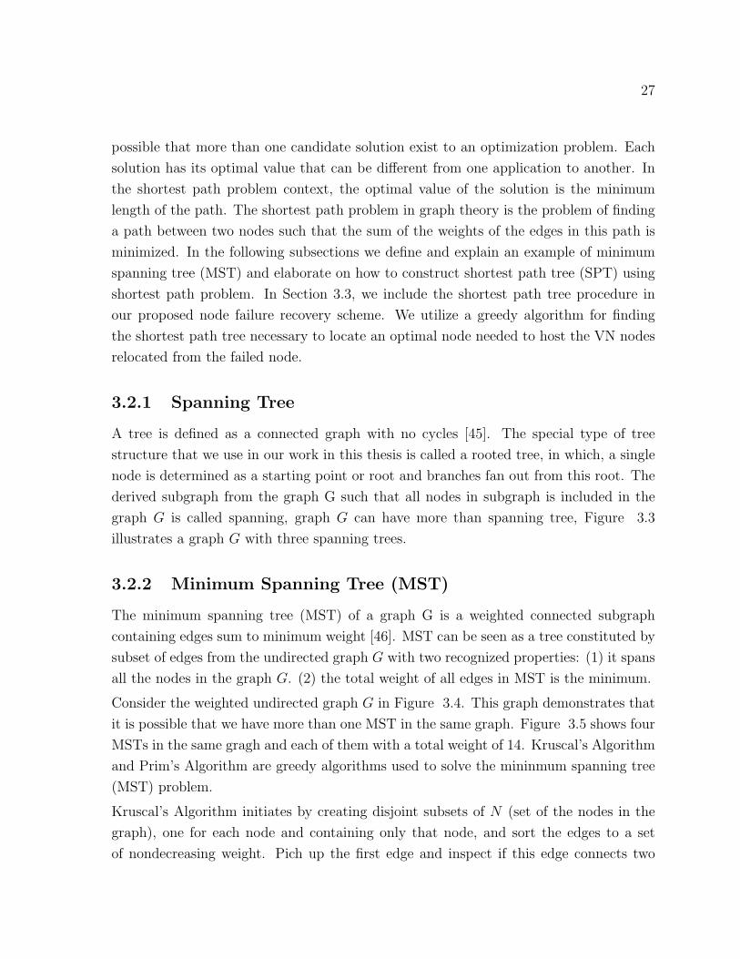
3.3 Graph G with three spanning trees (B,C and D) [45] . . . . . . . . . . . . . . . . 28

3.4 An undirected and weighted graph G [47] . . . . . . . . . . . . . . . . . . . . . 28

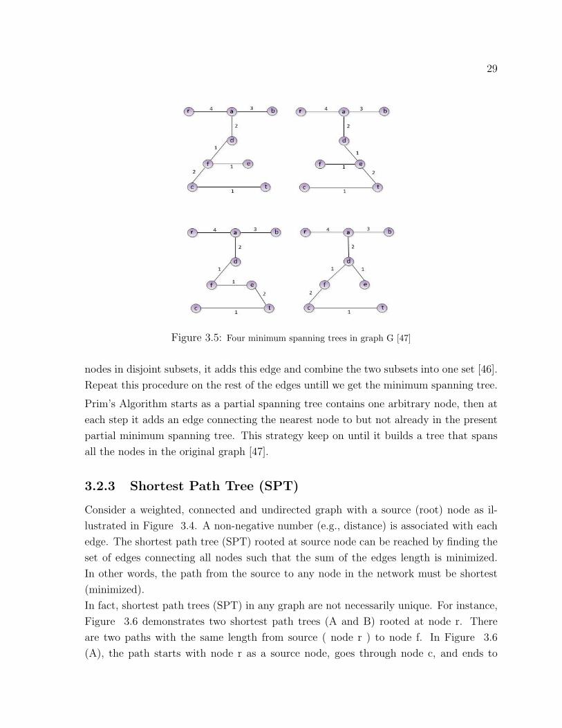
3.5 Four minimum spanning trees in graph G [47] . . . . . . . . . . . . . . . . . . . 29

3.6 Two shortest path trees in graph G [47] . . . . . . . . . . . . . . . . . . . . . . 30

3.7 A Graph G with one VN mapped and single failed node (node l) . . . . . . . . . . 31

3.8 The Graph G with the first root (node a) . . . . . . . . . . . . . . . . . . . . . 33

3.9 Choosing the root in SPT1 construction . . . . . . . . . . . . . . . . . . . . . . 33

3.10 Second step in the SPT1 construction process . . . . . . . . . . . . . . . . . . . 34

3.11 Choosing node m for SPT1 construction . . . . . . . . . . . . . . . . . . . . . . 34

3.12 Choosing node i for SPT1 construction . . . . . . . . . . . . . . . . . . . . . . 35

3.13 Choosing node d for SPT1 construction . . . . . . . . . . . . . . . . . . . . . . 35

3.14 Choosing node h for SPT1 construction . . . . . . . . . . . . . . . . . . . . . . 36

3.15 Choosing node c for SPT1 construction . . . . . . . . . . . . . . . . . . . . . . 36

3.16 Choosing node e for SPT1 construction . . . . . . . . . . . . . . . . . . . . . . 37

3.17 Choosing node n for SPT1 construction . . . . . . . . . . . . . . . . . . . . . . 37

3.18 Choosing node g for SPT1 construction . . . . . . . . . . . . . . . . . . . . . . 38

3.19 Choosing node b for SPT1 construction . . . . . . . . . . . . . . . . . . . . . . 38

3.20 Choosing node k for SPT1 construction . . . . . . . . . . . . . . . . . . . . . . 39

3.21 Choosing node f for SPT1 construction . . . . . . . . . . . . . . . . . . . . . . 39

3.22 SPT1 construction is completed for root a . . . . . . . . . . . . . . . . . . . . . 40

3.23 SPT2 construction at the second root (node b) . . . . . . . . . . . . . . . . . . 41

3.24 Choosing node e in graph G . . . . . . . . . . . . . . . . . . . . . . . . . . . 42

vi

3.25 Choosing node k in graph G . . . . . . . . . . . . . . . . . . . . . . . . . . . 42

3.26 Choosing node n in graph G . . . . . . . . . . . . . . . . . . . . . . . . . . . 43

3.27 Choosing node g in graph G . . . . . . . . . . . . . . . . . . . . . . . . . . . 43

3.28 Choosing node c in graph G . . . . . . . . . . . . . . . . . . . . . . . . . . . 44

3.29 Choosing node f in graph G . . . . . . . . . . . . . . . . . . . . . . . . . . . 44

3.30 Choosing node h in graph G . . . . . . . . . . . . . . . . . . . . . . . . . . . 45

3.31 Choosing node a in graph G . . . . . . . . . . . . . . . . . . . . . . . . . . . 45

3.32 Choosing node i in graph G . . . . . . . . . . . . . . . . . . . . . . . . . . . . 46

3.33 Choosing node m in graph G . . . . . . . . . . . . . . . . . . . . . . . . . . . 46

3.34 Choosing node j in graph G . . . . . . . . . . . . . . . . . . . . . . . . . . . . 47

3.35 Choosing node d in graph G . . . . . . . . . . . . . . . . . . . . . . . . . . . 47

3.36 The resulting SPT2 rooted at b in graph G . . . . . . . . . . . . . . . . . . . . 48

3.37 δ(ns) computation . . . . . . . . . . . . . . . . . . . . . . . . . . . . . . . . 48

3.38 σ(ns) computation . . . . . . . . . . . . . . . . . . . . . . . . . . . . . . . . 49

4.1 Average VN node degree vs. time taken for VN node relocation . . . . . . . . . . 57

4.2 Average VN node degree vs. success rate . . . . . . . . . . . . . . . . . . . . . 58

4.3 Average VN node degree vs. cost (allocated bandwidth) . . . . . . . . . . . . . . 59

4.4 Execution time against VN arrival rate . . . . . . . . . . . . . . . . . . . . . . 60

4.5 VN acceptance rate versus VN arrival rate . . . . . . . . . . . . . . . . . . . . . 61

4.6 Recovery success rate versus time (proposed approach) . . . . . . . . . . . . . . . 62

4.7 Recovery success rate versus time (Star-shaped VN component migration technique) . 63

4.8 Cost versus time (proposed approach) . . . . . . . . . . . . . . . . . . . . . . . 63

4.9 Cost versus time (Star-shaped VN component migration technique) . . . . . . . . . 64

4.10 Profit versus time (proposed approach) . . . . . . . . . . . . . . . . . . . . . . 64

4.11 Profit versus time (Star-shaped VN component migration technique) . . . . . . . . 65

vii

1

Acronyms

InP Infrastructure Network Provider

ISP Internet Service Provider

LAN Local Area Network

MST Minimum Spanning Tree

SLA Service Level Agreement

SN Substrate Network

SP Service Provider

SPT Shortest Path Tree

SVNE Survivable Virtual Network Embedding

VPN Virtual Private Network

VN Virtual Network

VNE Virtual Network Environment

VNR Virtual Network Reconfiguration

VLAN Virtual Local Area Network

WAN Wide Area Network

Chapter 1

Introduction

1.1 Introduction

The Internet’s stunning success has changed the way that people communicate and pro-

vided the effective environment for a multitude of business. However, the necessary

Internet growth has been unfortunately bounded by reliability constraints and social-

economic factors [1–4]. The implementation of any new architecture needs consensus

between ISPs. Network virtualization is introduced as a promising attribute to overcome

the above challenges and facilitate service deployment of the future inter-networking

environment [3–5].

Network virtualization is a powerful paradigm that allows multiple heterogeneous virtual

networks (VN) to efficiently share the resources in a single physical network infrastruc-

ture. Network virtualization brings several benefits to different applications. For in-

stance, multiple new network protocols or experiments can be evaluated simultaneously

in single shared substrate physical network [6].

A Virtual Network (VN) is composed of a group of virtual nodes that are hosted on their

unique substrate nodes, and are connected by virtual links that are mapped on substrate

paths [7]. Service providers (SPs) would lease resources (i.e., nodes and links) from one

or multiple infrastructure network providers(InPs) to create virtual networks and deploy

customized protocols to offer end-to-end services to the end users. A service provider

might also create child virtual networks by partitioning its resources to be leased to other

service providers [3].

A major challenge in the network virtualization context is how to efficiently use the

substrate resources (i.e., nodes CPU and links bandwidth). Mapping of virtual nodes

2

3

and virtual links onto the substrate resources is known to be an NP-hard problem [8],

even when virtual nodes are mapped already to the substrate nodes, mapping virtual

links into substrate paths is still NP-hard when the paths are unsplitable [9].

Several research efforts [10–15] addressing this challenge have been presented; a number

of these efforts introduced different heuristics to solve the problem of VN mapping in the

hopes of establishing efficient use of the substrate resources.

In addition to the heuristics needed to efficiently map the VNs in the substrate net-

work, we need techniques that manage the resources already allocated to active VNs.

Unfortunately, the literature still lacks such techniques. For instance, the infrastructure

provider (InP) may need to perform maintenance tasks for some substrate nodes and this

will require all hosted VN nodes to be migrated to other nodes in the physical network.

Clearly, if the service interruption time due to migration is too long, this operation will

cause service level agreement (SLA) violation. Furthermore, solving the problem of effi-

cient mapping of VNs in substrate network (SN) without taking into consideration the

effect of substrate node failure could decrease the InP revenue. Hence, there is a need to

develop a technique that can relocate the already hosted virtual nodes in case of node

failure or node maintenance while minimizing the relocation cost and service disruption

period.

1.2 Contribution

We introduce a novel distributed node failure recovery algorithm [16] that efficiently

reembeds the virtual nodes affected by a failed substrate node. The proposed scheme

relies on the cooperation of set of distributed managers hosted on a number of substrate

nodes to achieve this task. The process is triggered by the arrival of a substrate node

failure message from the InP. A designated manager node sends a request to the substrate

nodes hosting the neighbour nodes of the affected virtual nodes to search for a new

candidate substrate node. The search is performed by constructing shortest path trees

(SPT) from the neighboring nodes to all candidate nodes within a specific distance in the

SN. The calculated SPTs are then employed to find the optimal candidate node. The

proposed work efficiently reduces the experienced delay, service interruption time and

node failure relocation cost during this process while maximizing the InP revenue. By

applying this approach we establish the following:

4

• Reducing the time delay for recovering the substrate node from its failure by relo-

cating only the virtual nodes hosted in the failed node, and without relocating the

whole VN that possesses the virtual node hosted in the failed node.

• Lowering the cost in terms of the amount of bandwidth allocated to the affected

virtual links when relocating virtual nodes hosted on the failed node.

• Minimizing the service interruption period by reducing the time needed to recover

the failed node.

• Maximizing the InP revenue and reducing the penalty charges.

1.3 Thesis Structure

The rest of this thesis is organized as follows. In Chapter 2, network virtualization

background and related work is presented to review the literature and show how our

work is different from existing research. In Chapter 3, we formalize the node failure

recovery problem and describe the proposed scheme, and then we explain the shortest

path tree algorithm in our proposed approach. The performance evaluation of our work

is provided in Chapter 4. Finally, the conclusion and future work are presented in

Chapter 5.

Chapter 2

Background and Related Work

In this chapter we present the technologies that are relevant to network virtualization, and

describe related work in the literature. First, in Section 2.1 we begin with a background

about the virtual network environment (VNE), where we focus more into the systems

that use the concept of virtualization in their capacities. In Section 2.2, we define the

business model used in virtual network environment (VNE) and identify the important

business actors and their relations. We then demonstrate, in Section 2.3, the virtual

network (VN) mapping problem and explain the models of substrate network (SN) and

virtual network (VN). We explore, in Section 2.4, the previous work related to the VN

reconfiguration, re-optimization and survivability used in VNE. These mechanisims are

important to efficiently allocate sufficient resources to multiple virtual networks over

single substrate network, improve the performance of embedded virtual networks, and

increase the profit of the infrastructure provider (InP) in the VNE model.

2.1 Historical Background of VNE

The concept of network virtualization has been in the industry and academia communities

since quite some time. Its emergence is necessary to improve the performance of the

network and to face the challenges of internet ossification. In this section, we will briefly

discuss some capacities that network virtualization operates on and explore featurs and

objectives it aims to reach. Although all systems in virtualization context target different

purposes, they all aim at improving the Internet peformance as a common goal.

5

6

Virtual Local Area Network (VLAN)

A virtual local area network (VLAN) [17, 18] is a group of logically networked end-

stations, and perhaps multiple LAN segments in a single broadcast domain regardless of

their physical locations. VLAN is used to reach better security, improved performance,

and simplified administration. Based on the way in which VLAN membership can be

defined, the VLAN can be classified to the following types: Layer 1 VLAN (port group-

ing), Layer 2 VLAN (MAC-layer grouping), Layer 2 VLAN (Membership by Protocol),

Layer 3 VLAN (Membership by IP Subnet Address).

Virtual Private Network (VPN)

A virtual private network (VPN) [3,19–21] is a communication environment using the in-

ternet or any intermediate network (e.g., LAN/WAN) to connect multiple geographically

distributed sites (i.e., enterprises) using a non private IP data network to carry traffic

between them. Typically, sites that receive the VPN services can be Intranet, where

all the sites belong to the same enterprise, or Extranet, where sites belong to multiple

enterprises.

Programmable and Active Networks

The ability to rapidly create, deploy and manage novel services in response to user

demands is a prominont factor that attract the programmable networking research com-

munity [22]. Two separate schools of thought adopt the implementation of the concepts

of programmable and active networks:

• Open Signaling Approach: this is advocated by the opensig community [23], which

was established through a series of international workshops. The opensig commu-

nity argues that providing an open access to switches and routers can be established

by modeling communication hardware using a set of open programmable network

interfaces. By opening up the switches in this way, the development of new and

distinct architecture and services can be realized [22,23].

• Active Networks Approach [24–27]: this approach is adopted by the Defense Ad-

vanced Research Projects Agency (DARPA) research community in 1994 and 1995.

They introduced active networks approach to address the problem of the difficulty

of integrating new technologies and standards into shared network infrastructure,

and difficulty of accommodating new services in the existing architectural model.

7

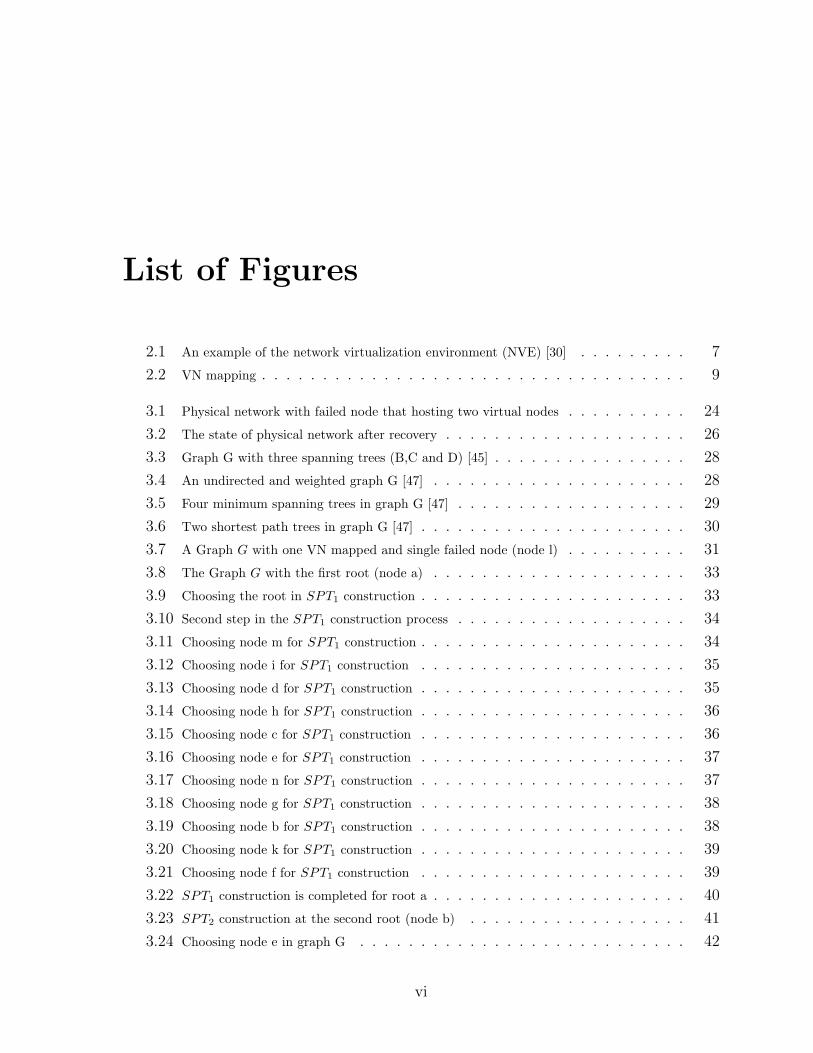
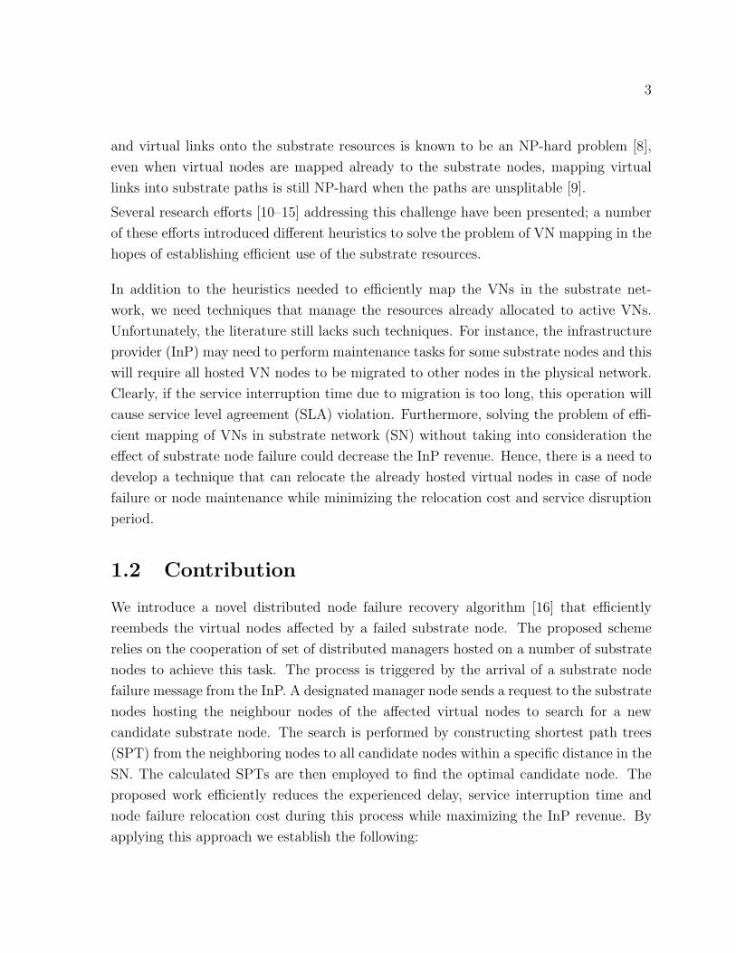
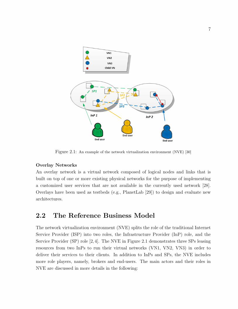
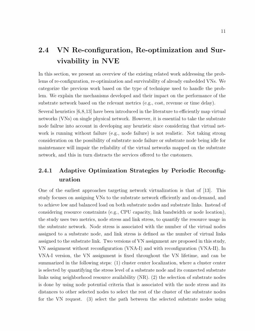
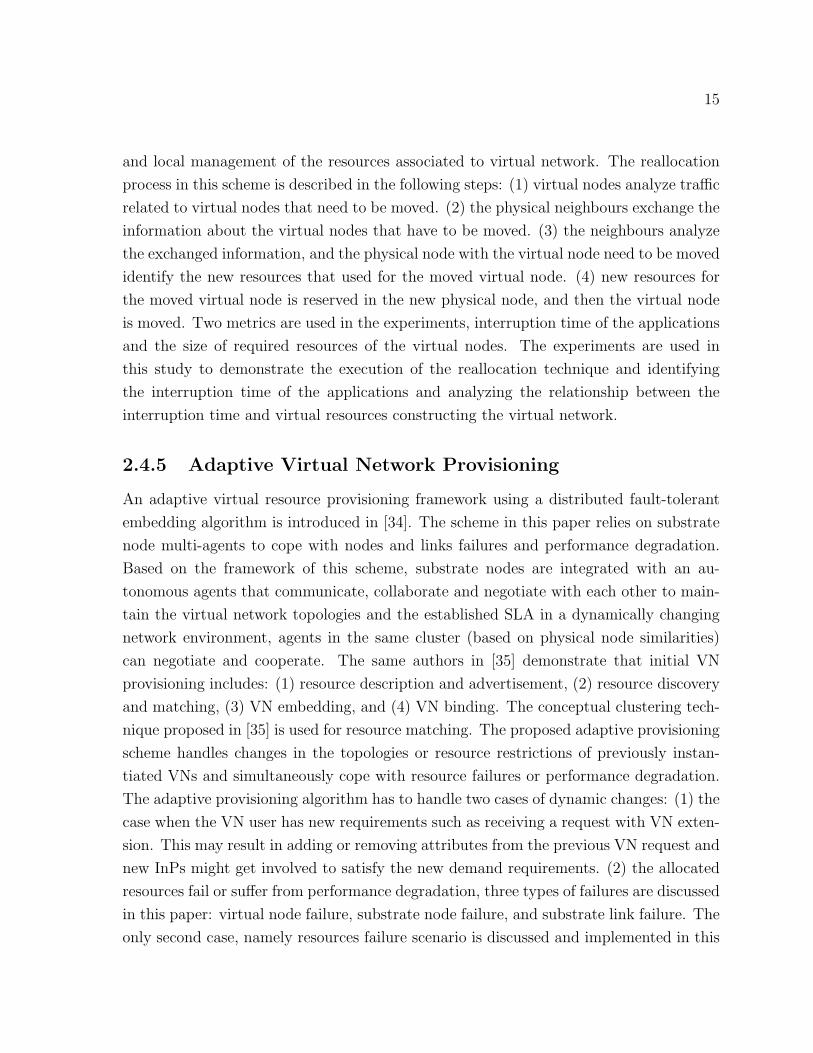
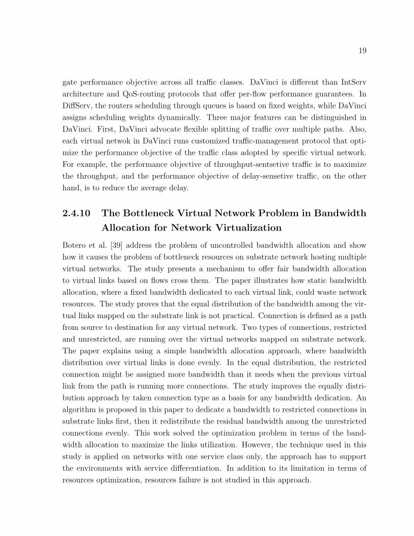
Figure 2.1: An example of the network virtualization environment (NVE) [30]

Overlay Networks

An overlay network is a virtual network composed of logical nodes and links that is

built on top of one or more existing physical networks for the purpose of implementing

a customized user services that are not available in the currently used network [28].

Overlays have been used as testbeds (e.g., PlanetLab [29]) to design and evaluate new

architectures.

2.2 The Reference Business Model

The network virtualization environment (NVE) splits the role of the traditional Internet

Service Provider (ISP) into two roles, the Infrastructure Provider (InP) role, and the

Service Provider (SP) role [2,4]. The NVE in Figure 2.1 demonstrates three SPs leasing

resources from two InPs to run their virtual networks (VN1, VN2, VN3) in order to

deliver their services to their clients. In addition to InPs and SPs, the NVE includes

more role players, namely, brokers and end-users. The main actors and their roles in

NVE are discussed in more details in the following:

8

Infrastructure Providers (InPs)

InPs are the main stakeholders in the network virtualization environment, they gain

revenue as a return to leasing physical resources to the service providers (SP) for a period

of time and based on agreement between both two parties. Along with accepting and

deploying new VN requests, InPs are responsible for physical resources maintenance and

management, for instance fixing the physical resources in failure times. InPs accepting

new VN requests that capitalize their revenue with lower cost of deploying those VNs.

Multiple InPs can interact and collaborate to accept and deploy more VN requests based

on defined terms and policies that govern their relationship.

Service Providers (SPs)

A Service Provider leases physical resources (e.g., nodes and links) from the infrastruc-

ture provider to create a virtual network (VN), with customized protocols, that provide

end-to-end services to the end users (customers), i.e., VN1, VN2, and VN3 in Figure 2.1

are created by SP1, SP2, and SP3 respectively. One or multiple infrastructure providers

might involve in creating one virtual network owned by specific service provider. Ac-

cepting or rejecting a new virtual network request depends on the availability of the

physical resources in the network, VN cost and revenue and the constraints satisfaction

of VN request. Upon instantiation of virtual network on one or multiple InPs, terms

and policies are defind in service level agreement(SLA) to make sure that InP and SP

requirements are met. Any SP could create multiple virtual networks (child VNs) from

its original virtual network and lease them to other service providers, i.e., VN3 creates

one child VN in Figure 2.1.

End-Users

The end-user in the network virtualization environment (NVE) context is one of the

main stakeholders that uses the service offered by service provider. By offering a variety

of services from different competing service providers, the end-users might choose one

among them based on their preference in terms of service price and quality. The services

are offered on the basis of terms and policies between the end-users and service providers

defined on the service level agreement (SLA). End-users consult brokers to help them

find their target of service, and they might access one or multiple service providers.

9

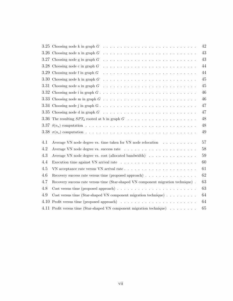
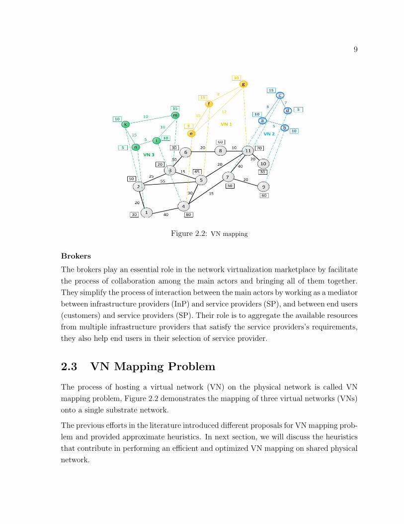
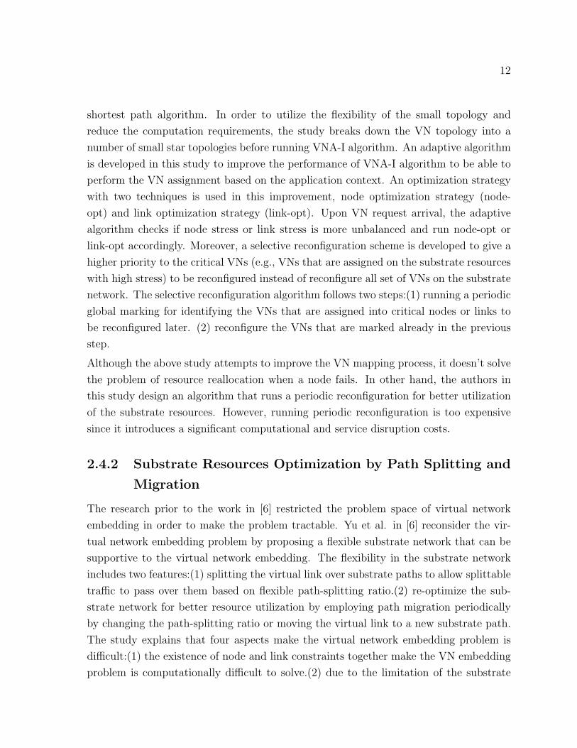
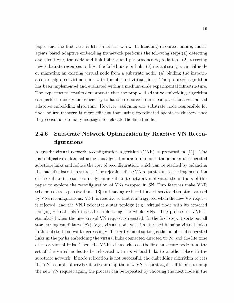
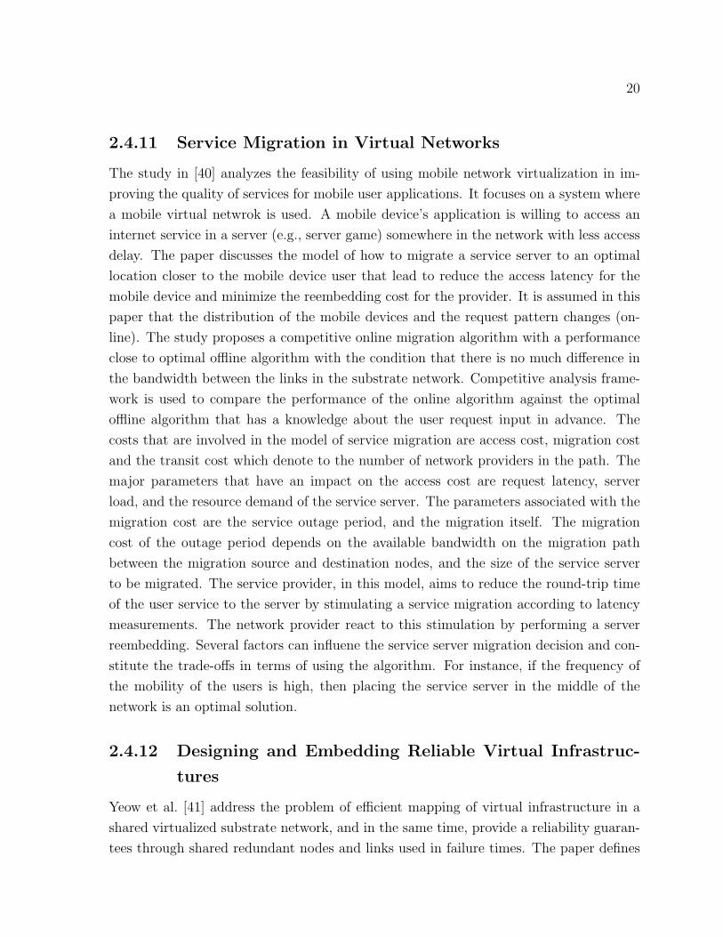
Figure 2.2: VN mapping

Brokers

The brokers play an essential role in the network virtualization marketplace by facilitate

the process of collaboration among the main actors and bringing all of them together.

They simplify the process of interaction between the main actors by working as a mediator

between infrastructure providers (InP) and service providers (SP), and between end users

(customers) and service providers (SP). Their role is to aggregate the available resources

from multiple infrastructure providers that satisfy the service providers’s requirements,

they also help end users in their selection of service provider.

2.3 VN Mapping Problem

The process of hosting a virtual network (VN) on the physical network is called VN

mapping problem, Figure 2.2 demonstrates the mapping of three virtual networks (VNs)

onto a single substrate network.

The previous efforts in the literature introduced different proposals for VN mapping prob-

lem and provided approximate heuristics. In next section, we will discuss the heuristics

that contribute in performing an efficient and optimized VN mapping on shared physical

network.

10

2.3.1 Network Model

Substrate Network

The previous work in [8] models the substrate network SN as an undirected weighted

graph denoted by Gs = (Ns, Ls) , where Ns is a set of substrate nodes, Ls is a set of

substrate links. Each substrate node ns ∈ Ns is characterized by its CPU capacity which

is denoted by cpu(ns), and each substrate link ls ∈ Ls is associated with its bandwidth

capacity bw(ls), Figure 2.2 illustrates the CPU and bandwidth capacities of the substrate

nodes and links respectively in graph G.

VN Request

A virtual network request (VN ) is represented as an undirected weighted graph Gv =

(Nv, Lv) , where Nv is a set of virtual nodes nv associated with their CPU requirements

cpu(nv) that must be satisfied, and Lv is a set of virtual links lv, each of which has its

bandwidth demand bw(lv) to be met in any VN mapping, Figure 2.2 shows three VNs

( VN1, VN2 and VN3) with their resources requirements ( i.e, CPU and bandwidth )

that have to be satisfied when mapped in a single substrate network.

Node and Link Mapping

The VN mapping process is comprised of two phases [8] [13]: Node mapping ( MN :

Nv → Ns ) and Link mapping (ML : Lv → Ps ), where Ps is a set of substrate paths.

Each virtual link can be mapped onto an unsplittable substrate path or a set of splittable

substrate paths [8].

After a VN is deployed, the remaining capacity of the substrate resources is referred

to the residual cpu capacity cpures(ns) of the substrate nodes and the residual band-

width capacity bwres(ls) of the substrate links. Those two variables (i.e., cpures(ns) and

bwres(ls) ) are two factors used to indicate the load of the physical network [6].

Having described the VN embedding process, we next discuss multiple systems and

techniques in terms of VN reconfiguration, re-optimization and survivability developed

in the prior work in the literature. We explore their pros and cons and how the previous

work related to the VN reconfiguration, re-optimization and survivability used in VNE.

11

2.4 VN Re-configuration, Re-optimization and Sur-

vivability in NVE

In this section, we present an overview of the existing related work addressing the prob-

lems of re-configuration, re-optimization and survivability of already embedded VNs. We

categorize the previous work based on the type of technique used to handle the prob-

lem. We explain the mechanisms developed and their impact on the performance of the

substrate network based on the relevant metrics (e.g., cost, revenue or time delay).

Several heuristics [6,8,13] have been introduced in the literature to efficiently map virtual

networks (VNs) on single physical network. However, it is essential to take the substrate

node failrue into account in developing any heuristic since considering that virtual net-

work is running without failure (e.g., node failure) is not realistic. Not taking strong

consideration on the possibility of substrate node failure or substrate node being idle for

maintenance will impair the reliability of the virtual networks mapped on the substrate

network, and this in turn distracts the services offered to the customers.

2.4.1 Adaptive Optimization Strategies by Periodic Reconfig-

uration

One of the earliest approaches targeting network virtualization is that of [13]. This

study focuses on assigning VNs to the substrate network efficiently and on-demand, and

to achieve low and balanced load on both substrate nodes and substrate links. Instead of

considering resource constraints (e.g., CPU capacity, link bandwidth or node location),

the study uses two metrics, node stress and link stress, to quantify the resource usage in

the substrate network. Node stress is associated with the number of the virtual nodes

assigned to a substrate node, and link stress is defined as the number of virtual links

assigned to the substrate link. Two versions of VN assignment are proposed in this study,

VN assignment without reconfiguration (VNA-I) and with reconfiguration (VNA-II). In

VNA-I version, the VN assignment is fixed throughout the VN lifetime, and can be

summarized in the following steps: (1) cluster center localization, where a cluster center

is selected by quantifying the stress level of a substrate node and its connected substrate

links using neighborhood resource availability (NR). (2) the selection of substrate nodes

is done by using node potential criteria that is associated with the node stress and its

distances to other selected nodes to select the rest of the cluster of the substrate nodes

for the VN request. (3) select the path between the selected substrate nodes using

12

shortest path algorithm. In order to utilize the flexibility of the small topology and

reduce the computation requirements, the study breaks down the VN topology into a

number of small star topologies before running VNA-I algorithm. An adaptive algorithm

is developed in this study to improve the performance of VNA-I algorithm to be able to

perform the VN assignment based on the application context. An optimization strategy

with two techniques is used in this improvement, node optimization strategy (node-

opt) and link optimization strategy (link-opt). Upon VN request arrival, the adaptive

algorithm checks if node stress or link stress is more unbalanced and run node-opt or

link-opt accordingly. Moreover, a selective reconfiguration scheme is developed to give a

higher priority to the critical VNs (e.g., VNs that are assigned on the substrate resources

with high stress) to be reconfigured instead of reconfigure all set of VNs on the substrate

network. The selective reconfiguration algorithm follows two steps:(1) running a periodic

global marking for identifying the VNs that are assigned into critical nodes or links to

be reconfigured later. (2) reconfigure the VNs that are marked already in the previous

step.

Although the above study attempts to improve the VN mapping process, it doesn’t solve

the problem of resource reallocation when a node fails. In other hand, the authors in

this study design an algorithm that runs a periodic reconfiguration for better utilization

of the substrate resources. However, running periodic reconfiguration is too expensive

since it introduces a significant computational and service disruption costs.

2.4.2 Substrate Resources Optimization by Path Splitting and

Migration

The research prior to the work in [6] restricted the problem space of virtual network

embedding in order to make the problem tractable. Yu et al. in [6] reconsider the vir-

tual network embedding problem by proposing a flexible substrate network that can be

supportive to the virtual network embedding. The flexibility in the substrate network

includes two features:(1) splitting the virtual link over substrate paths to allow splittable

traffic to pass over them based on flexible path-splitting ratio.(2) re-optimize the sub-

strate network for better resource utilization by employing path migration periodically

by changing the path-splitting ratio or moving the virtual link to a new substrate path.

The study explains that four aspects make the virtual network embedding problem is

difficult:(1) the existence of node and link constraints together make the VN embedding

problem is computationally difficult to solve.(2) due to the limitation of the substrate

13

resources, the admission control is used to accept, reject or postpone any new VN request

based on the substrate resources workload.(3) the arrival and departure of the virtual

networks are dynamic.(4) the topology of the virtual network is diverse and not known

in advance. Previous research considered one or some of these aspects to propose a new

efficient heuristics that solve VN embedding problem. This study, on the other hand,

satisfy the first three features above by allowing a flexible path splitting and migration,

and address the fourth feature by developing a customized node-embedding algorithm

for a hub-and-spoke topology. A VN mapping heuristic that aims to maximize the InP

revenue is introduced in this study as a baseline algorithm that is used for path splitting

and migration approaches. The algorithm orders the arriving virtual netwok requests

within the time window decreasingly based on their revenues and processes all the VN

requests by first mapping the virtual nodes into the substrate nodes using a greedy al-

gorithm for all considered VN requests, then map the virtual links of those considered

VNs into the substrate links using k-shortest path algorithm. VN requests would not

be mapped on the substrate netwok are sent to the request queue to be reconsidered

later. The study argues that path splitting and migration should be considered in the

future virtualization network for the following reasons: it enables better resources utiliza-

tion that allow accepting more VN requests, flexible path splitting makes link mapping

computationally tractable, load balancing, reliability and faster recovery from network

failures. The study proposed some techniques to prevent the performance disruption,

for example, hash-based splitting is used to prevent the out of order delivery, adding

some artificial delay by substrate provider to prevent the variable probogation delay and

tagging the packets with a sequence numbers.

The authors in this paper introduce a centralized mapping scheme in which a single

entity (e.g., InP) has a global knowledge about whole substrate network, and this entity

playing the major role of accepting/rejecting new VNs. However, the existence of the

centralized entity (e.g., admission control) impairs the network scability which is one of

the most important challenges that network virtualization emerged for. Furthermore,

although the paper doesn’t consider the node failure, if we have the node failure as one

of the events handled in this approach there will be a delay introduced in node failure

recovery due to the existence of admission control.

14

2.4.3 Topology-based Virtual Network Mapping

In [31], authors propose a model on how to map VNs onto the substrate network in a

least-cost way, while allocating sufficient bandwidth to the VN links that enable them to

handle any pattern of traffic in accordance with a set of constraints. The approach at-

tempts to choose the best topology in the family of backbone-star topologies that satisfy

set of traffic constraints. In backbone-star topologies, there are a subset of backnbone

nodes that constitute the VN backbone, which is formed as a complete graph, a ring or

a star. The remaining nodes, that are called access nodes, are connected to the nearest

backbone nodes via a single link. Along with distance-based constraints that bound the

amount of traffic between each node and its more distant peers, and similar to those in

the hose model [32], authors specify traffic using a combination of pairwise constraints

and termination constraints. The iterative process used in this approach to reach the

best mapping is as the following: (1) select an initial mapping of backbone nodes onto

the substrate network. (2) connect each access node to the closest backbone node. (3)

compute shortest paths between the backbone nodes and access nodes using the defined

links lengths. (4) determine link capacities using maximum flow computations. (5) ex-

plore alternative mappings of backbone nodes onto the substrate network. This iterative

process is terminated when it is not likely getting more improvements in next steps solu-

tion or when reach the pre-defined number of iterations limit. The VN configuration cost

is defined as a Mixed Integer Quadratic Programming (MIQP) problem. The objective

function in this model has to be minimized to reach the goal of least-cost VN mapping.

Although this study develops a cost-effective method for VN mapping in the substrate

network, which is essential, the resources survivability is missing in their work.

2.4.4 Distributed Reallocation for Virtual Network Resources

In [33], a virtual network resources reallocation scheme with a real-time distributed based

algorithm is proposed. A self-organizing technique is defined to migrate one virtual node

with its resources from one physical node to another in order to maximize the utilization

of the physical resources. This reallocation is executed by virtual managers inside each

physical node. An IPTV testbed scenario is adopted and Omnet++ simulator is used

to test their proposed system in terms of the IPTV services’ disruption. The paper

describes that a physical node as a node that consists of: physical resources, virtual

nodes and virtual pipes. The major management tasks are dedicated to the virtual

node, the tasks include handling the requests for deployment of a virtual node or pipe

15

and local management of the resources associated to virtual network. The reallocation

process in this scheme is described in the following steps: (1) virtual nodes analyze traffic

related to virtual nodes that need to be moved. (2) the physical neighbours exchange the

information about the virtual nodes that have to be moved. (3) the neighbours analyze

the exchanged information, and the physical node with the virtual node need to be moved

identify the new resources that used for the moved virtual node. (4) new resources for

the moved virtual node is reserved in the new physical node, and then the virtual node

is moved. Two metrics are used in the experiments, interruption time of the applications

and the size of required resources of the virtual nodes. The experiments are used in

this study to demonstrate the execution of the reallocation technique and identifying

the interruption time of the applications and analyzing the relationship between the

interruption time and virtual resources constructing the virtual network.

2.4.5 Adaptive Virtual Network Provisioning

An adaptive virtual resource provisioning framework using a distributed fault-tolerant

embedding algorithm is introduced in [34]. The scheme in this paper relies on substrate

node multi-agents to cope with nodes and links failures and performance degradation.

Based on the framework of this scheme, substrate nodes are integrated with an au-

tonomous agents that communicate, collaborate and negotiate with each other to main-

tain the virtual network topologies and the established SLA in a dynamically changing

network environment, agents in the same cluster (based on physical node similarities)

can negotiate and cooperate. The same authors in [35] demonstrate that initial VN

provisioning includes: (1) resource description and advertisement, (2) resource discovery

and matching, (3) VN embedding, and (4) VN binding. The conceptual clustering tech-

nique proposed in [35] is used for resource matching. The proposed adaptive provisioning

scheme handles changes in the topologies or resource restrictions of previously instan-

tiated VNs and simultaneously cope with resource failures or performance degradation.

The adaptive provisioning algorithm has to handle two cases of dynamic changes: (1) the

case when the VN user has new requirements such as receiving a request with VN exten-

sion. This may result in adding or removing attributes from the previous VN request and

new InPs might get involved to satisfy the new demand requirements. (2) the allocated

resources fail or suffer from performance degradation, three types of failures are discussed

in this paper: virtual node failure, substrate node failure, and substrate link failure. The

only second case, namely resources failure scenario is discussed and implemented in this

16

paper and the first case is left for future work. In handling resources failure, multi-

agents based adaptive embedding framework performs the following steps:(1) detecting

and identifying the node and link failures and performance degradation. (2) reserving

new substrate resources to host the failed node or link. (3) instantiating a virtual node

or migrating an existing virtual node from a substrate node. (4) binding the instanti-

ated or migrated virtual node with the affected virtual links. The proposed algorithm

has been implemented and evaluated within a medium-scale experimental infrastructure.

The experimental results demonstrate that the proposed adaptive embedding algorithm

can perform quickly and efficiently to handle resource failures compared to a centralized

adaptive embedding algorithm. However, assigning one substrate node responsible for

node failure recovery is more efficient than using coordinated agents in clusters since

they consume too many messages to relocate the failed node.

2.4.6 Substrate Network Optimization by Reactive VN Recon-

figurations

A greedy virtual network reconfiguration algorithm (VNR) is proposed in [11]. The

main objectives obtained using this algorithm are to minimise the number of congested

substrate links and reduce the cost of reconfiguration, which can be reached by balancing

the load of substrate resources. The rejection of the VN requests due to the fragmentation

of the substrate resources in dynamic substrate network motivated the authors of this

paper to explore the reconfiguration of VNs mapped in SN. Two features make VNR

scheme is less expensive than [13] and having reduced time of service disruption caused

by VNs reconfigurations: VNR is reactive so that it is triggered when the new VN request

is rejected, and the VNR relocates a star toplogy (e.g., virtual node with its attached

hanging virtual links) instead of relocating the whole VNs. The process of VNR is

stimulated when the new arrival VN request is rejected. In the first step, it sorts out all

star moving candidates {Ni} (e.g., virtual node with its attached hanging virtual links)

in the substrate network decreasingly. The criterion of sorting is the number of congested

links in the paths embedding the virtual links connected directed to Ni and the life time

of those virtual links. Then, the VNR scheme chooses the first substrate node from the

set of the sorted nodes to be relocated with its virtual links to anothor place in the

substrate network. If node relocation is not successful, the embedding algorithm rejects

the VN request, otherwise it tries to map the new VN request again. If it fails to map

the new VN request again, the process can be repeated by choosing the next node in the

17

sorted list until it succeed or a maximum number of allowed iterations is reached(Nmig).

2.4.7 Topology-Awareness and Reoptimization Mechanism for

Virtual Network Embedding

The differentiating between substrate resources is used as a mechanism in [12] for solving

VN mapping problem efficiently. Also, a new re-optimization technique is developed in

this study to accept any new rejected VN by fixing the bottleneck substrate resources.

The designing of the differentiating technique is based on assigning weights to substrate

nodes and links according to their residual capacity and their importance in the sub-

strate network. This mechanism allows informed decisions while mapping VNs onto the

substrate resources on critical nodes and links. The study uses the scaling factor (SF) to

the costs of the substrate resources to differentiate between them, this SF refers to their

likelihood of becoming bottleneck. SF is calculated as a linear combination of critical

index (CI) and popularity index (PI). CI of the substrate resource is used to measure

the likelihood of a residual substrate network partition due to its unavailability. Pop-

ularity index (PI) is the weighted average of used resources on links and nodes used

to measure the severity of substrate resources unavailability on the substrate network.

Furthermore, the re-optimization process used in this study follows two steps. In the

first step, the study uses two algorithms to detect the virtual resources (e.g., nodes and

links) that cause the rejection of the new virtual network request. In the second step, the

study uses two algorithms to relocate these virtual nodes/links to less critical substrate

resources in the network. The authors stress on better resources utilization and network

optimization in order to improve the overall VN acceptance ratio, however, they need

to elaborate on the VN network suvivability as well since it is important for network

optimization.

2.4.8 A Survivable Virtual Network Embedding (VNE)

Heuristic

Raihan et al. [9] addresses the substrate link failure by formulating survivable virtual

network embedding (SVNE) problem that incorporate a substrate link failures in VNE

and developing a hybrid policy heuristic to solve it. The algorithm is based on dedicating

a certain percentage of bandwidth resources on each substrate link for backup purposes.

The authors explain how their work in survivability in network virtualization is different

18

from survivability in other network technologies such as optical and multi-protocol label

switched (MPLS) networks. The VNE problem is on-line, while the survivable logical

topology design problem in Optical and MPLS networks is off-line. The other difference

is that each virtual link must stay operational in the presence of a link failure event,

however, this is not a constraint in the optical networks, where the goal is to ensure that

all virtual nodes are connected when failure occurs. The main objective of their work is

to introduce a survivable network embedding solution that can simultaneously maximize

the long term revenue gained by the InP and minimize the long term penalty charged

to InP for any service disruption caused by substrate link failures. Twofold objective

functions are formulated in a linear program, the first objective function corresponds

to the long term revenue earned by InP, and the second objective function refers to

the penalty paid by InP due to service violation. The proposed hybrid policy heuristic

follows three phases: (1) this phase initiates before the arrival of VN requests, the InP

pro-actively computes a set of backup detours for each substrate link using any path

selection technique. (2) in the second phase, which is triggered upon the arrival of VN

requests, the InP uses the existing node mapping algorithms [8] [13] to perform node

mapping and the multi-commodity flow based link embedding. (3) in the presence of a

substrate link failure, a backup detour optimization solution is triggered, this heuristic

changes the routes of the effected bandwitdh to pass over the candidate backup detours

selected earlier in the first phase. The last two policies are formulated in a linear program.

The VN resources survivablity includes both VN nodes and links survivability. There is

a limitation on this study since it presents approach that only survives failed links.

2.4.9 Dynamically Adaptive Virtual Networks

A simple and flexible architecture for supporting multiple traffic classes and efficiently

managing resources between multiple virtual networks is presentd in [36]. Optimization

is used to prove that adaptive resources allocation can bring the stability and improved

performance to the virtual networks. The study proposes the DaVinci (Dynamically

Adaptive Virtual Network for a Customized Internet) architecture in which each sub-

strate link periodically reassigns bandwidth shares between assigned virtual links based

on local information (e.g., current congestion level and the performance level of the virtual

network), and each virtual network runs its own customized packet-delivery protocol that

optimise its performance objective. Compared to traditional Quality-of-Service (QoS)

techniques, that aim to provide performance guarantees, DaVinci maximizes the aggre-

19

gate performance objective across all traffic classes. DaVinci is different than IntServ

architecture and QoS-routing protocols that offer per-flow performance guarantees. In

DiffServ, the routers scheduling through queues is based on fixed weights, while DaVinci

assigns scheduling weights dynamically. Three major features can be distinguished in

DaVinci. First, DaVinci advocate flexible splitting of traffic over multiple paths. Also,

each virtual netwok in DaVinci runs customized traffic-management protocol that opti-

mize the performance objective of the traffic class adopted by specific virtual network.

For example, the performance objective of throughput-sentsetive traffic is to maximize

the throughput, and the performance objective of delay-sensetive traffic, on the other

hand, is to reduce the average delay.

2.4.10 The Bottleneck Virtual Network Problem in Bandwidth

Allocation for Network Virtualization

Botero et al. [39] address the problem of uncontrolled bandwidth allocation and show

how it causes the problem of bottleneck resources on substrate network hosting multiple

virtual networks. The study presents a mechanism to offer fair bandwidth allocation

to virtual links based on flows cross them. The paper illustrates how static bandwidth

allocation, where a fixed bandwidth dedicated to each virtual link, could waste network

resources. The study proves that the equal distribution of the bandwidth among the vir-

tual links mapped on the substrate link is not practical. Connection is defined as a path

from source to destination for any virtual network. Two types of connections, restricted

and unrestricted, are running over the virtual networks mapped on substrate network.

The paper explains using a simple bandwidth allocation approach, where bandwidth

distribution over virtual links is done evenly. In the equal distribution, the restricted

connection might be assigned more bandwidth than it needs when the previous virtual

link from the path is running more connections. The study improves the equally distri-

bution approach by taken connection type as a basis for any bandwidth dedication. An

algorithm is proposed in this paper to dedicate a bandwidth to restricted connections in

substrate links first, then it redistribute the residual bandwidth among the unrestricted

connections evenly. This work solved the optimization problem in terms of the band-

width allocation to maximize the links utilization. However, the technique used in this

study is applied on networks with one service class only, the approach has to support

the environments with service differentiation. In addition to its limitation in terms of

resources optimization, resources failure is not studied in this approach.

20

2.4.11 Service Migration in Virtual Networks

The study in [40] analyzes the feasibility of using mobile network virtualization in im-

proving the quality of services for mobile user applications. It focuses on a system where

a mobile virtual netwrok is used. A mobile device’s application is willing to access an

internet service in a server (e.g., server game) somewhere in the network with less access

delay. The paper discusses the model of how to migrate a service server to an optimal

location closer to the mobile device user that lead to reduce the access latency for the

mobile device and minimize the reembedding cost for the provider. It is assumed in this

paper that the distribution of the mobile devices and the request pattern changes (on-

line). The study proposes a competitive online migration algorithm with a performance

close to optimal offline algorithm with the condition that there is no much difference in

the bandwidth between the links in the substrate network. Competitive analysis frame-

work is used to compare the performance of the online algorithm against the optimal

offline algorithm that has a knowledge about the user request input in advance. The

costs that are involved in the model of service migration are access cost, migration cost

and the transit cost which denote to the number of network providers in the path. The

major parameters that have an impact on the access cost are request latency, server

load, and the resource demand of the service server. The parameters associated with the

migration cost are the service outage period, and the migration itself. The migration

cost of the outage period depends on the available bandwidth on the migration path

between the migration source and destination nodes, and the size of the service server

to be migrated. The service provider, in this model, aims to reduce the round-trip time

of the user service to the server by stimulating a service migration according to latency

measurements. The network provider react to this stimulation by performing a server

reembedding. Several factors can influene the service server migration decision and con-

stitute the trade-offs in terms of using the algorithm. For instance, if the frequency of

the mobility of the users is high, then placing the service server in the middle of the

network is an optimal solution.

2.4.12 Designing and Embedding Reliable Virtual Infrastruc-

tures

Yeow et al. [41] address the problem of efficient mapping of virtual infrastructure in a

shared virtualized substrate network, and in the same time, provide a reliability guaran-

tees through shared redundant nodes and links used in failure times. The paper defines

21

the reliability as the probability that critical nodes remain in operation over all possi-

ble node failures. Guaranteeing a reliability of r, where r is the level of reliability, for

any virtual infrastructure, means that there are sufficient residual physical resources in

case of failures with a probability r. At each instantiation of virtual infrastructures, a

backup resources (e.g., virtual servers) with sufficient capacities are created to be used

by multiple virtual infrastructures in order to guarantee a level of reliability in case of

any physical failure. For better overall utilization of physical resources, the backup re-

sources are pooled and shared by multiple virtual infrastructures. The customized virtual

infrastructures with different levels of reliability over single shared physical network dy-

namically create and pool together the shared redundant virtual servers. Opportunistic

Redundancy Pooling michanism is used to develop the redundancy architecture discussed

in this paper. The number of the redundant nodes in the redundancy architecture de-

pends on the physical mapping and the failure models of the physical nodes and the

virtual infrastructure.

2.5 Survivability in Overlay Networks

Survivability in the overlay networks is essential since they are hosted on an unstable

underlay network environment in which resources are subject to fail. In fact, virtual

networks are similar to overlay networks since both are hosted on an underlay network.

On the other hand, network survivability in overlay networks is more studied in the

literature than network virtualization. Therefore, we discuss some algorithms used to

survive overlay networks affected by failed resources. These algorithms provide self-repair

techniques which are similar to our work.

Porter et al. [42] present an algorithm that runs a decentralized repair operation of failed

nodes in overlay networks. This algorithm is designed as a generic, flexible and robust

framework that is deployed to include different repair techniques used by the overlay

networks (e.g., large-scale distributed systems). The authors design a three-phases repair

technique that enables the border nodes of the failed section of the overlay network to

perform the following: (1) determining the extent of the crashed section (2) identifying

the repair coordinator (3) executing the repair procedure.

Stoica et al. [43] develop Chord, an algorithm for peer to peer distributed applications,

that deals with nodes joining the system and with nodes that leave or fail dynamically.

Chord is characterized with its simplicity, provable performance and proven correctness.

22

Chord solves the problem of locating a data item in a set of distributed nodes, considering

dynamic node arrivals and departures.

2.6 Discussion

The aforementioned approaches design algorithms for better utilization of substrate re-

sources. The main objective of the algorithms is to increase the InP revenue by accepting

more VNs. They design optimization heuristics that lead the substrate network to host

more VNs. Different reconfiguration algorithms that take different patterns (e.g., reac-

tive or proactive) are developed for re-mapping the VNs to enable the substrate network

to accept more VN requests.

One interesting observation is that the majority of existing approaches don’t consider

resource failure while they handle the VN embedding. Addressing the problem of re-

sources survivability is fundamental in VN mapping problem to maintain the reliability

of the services offered to the clients and to increase the InP revenue. Raihan et al. [9]

present a technique that solves the problem of substrate link failure, however, the node

failure recovery is another issue that need to be investigated further.

Furthermore, it is worth noting that most of the work in the literature focuses on design-

ing centralized mapping and optimization schemes. However, centralization might cause

delay and affect the network scalability since only one entity coordinates the mapping

and optimization processes.

In contrast, there are more research efforts in the literature in terms of resources surviv-

ability in overlay networks. Distributed algorithms for self-repair is presented in overlay

networks. For example, the authors in [42] present an algorithm that achieves decentral-

ized repair of failed nodes in large-scale distributed systems. However, these solutions

are not suitable for virtual networks.

In order to address the problems above, we create self-management nodes that are able

to manage the node failure recovery task. In Chapter 3, we develop a novel node failure

recovery scheme in a decentralized manner.

Chapter 3

SPT & Node Failure Recovery in

NVE

In this chapter, we introduce an overview of shortest path problem in network envi-

ronments in general and present the proposed node failure recovery scheme. In Section

3.1 we begin with defining the network model used in the proposed scheme and explain

the node failure recovery problem description. In Section 3.2, we define the spanning

tree algorithm and explain it with example. Then, we describe the shortest path tree

technique in more details. In Section 3.3, Dijkstra’s Algorithm used in our proposal is

explained with an example provided to show how it works. We present the proposed

recovery algorithm in Section 3.4. In Section 3.5, we extend the proposed solution to the

case of the node failure recovery in overloaded networks. Finally, we compute the time

complexity of the proposed node failure recovery approach in Section 3.6.

3.1 Network Model and Problem Description

3.1.1 Network Model

We extend the substrate network (SN) demonsterated in Section 2.3. The new substrate

network is modeled as an undirected weighted graph denoted by Gs = (Ns, Ls, Rs), where

Ns and Ls were explained in Section 2.3. Rs represents the set of manager nodes, where

Rs ⊆ Ns, that are responsible for running the proposed node failure recovery algorithm.

Each manager node is associated with one or more SN nodes in the physical network and

performs the steps necessary to recover from node failure. This assignment is decided by

23

24

VN ID Virtual node Capacity Adjacent nodes

1 a 20 x hosted on node 4

y hosted on node 8

2 b 20 f hosted on node 4

c hosted on node 1

Table 3.1: The maintained table by manager node 9 in Figure 3.1

Figure 3.1: Physical network with failed node that hosting two virtual nodes

the InP. The process of assigning the manager nodes and the criteria considered in the

selection of the manager nodes will be investigated in future work.

In our approach, we assume that the mapping of the VN requests has already been

performed and the manager nodes in the physical network are assigned in the mapping

phase.

Each manager node (e.g., node 9 in Figure 3.1 manages node 11) maintains a table (e.g.,

Table 3.1) that contains the IDs of the VNs having virtual nodes hosted on the managed

substrate node. Also, the table maintains references to the hosted VN nodes in the

substrate node (e.g., nodes a and b in Figure 3.1), and the adjacent virtual nodes to the

hosted nodes (e.g., nodes f and c in Figure 3.1). This table is updated continuously (e.g.,

every time a VN is accepted or rejected).

Figure 3.1 depicts an example of substrate network with two already embedded VNs.

The failed node (node 11) has been assigned a manager node (node 9) that is responsible

25

for VN nodes reallocation.

The InP’s revenue received from serving a VN request can be calculated as follows:

R(Gv) = T (Gv)(fcpu

∑nv∈Nv

cpu(nv) + fbw∑lv∈Lv

bw(lv))

(3.1)

Where T (Gv) represents the life-time of the hosted VN, Gv. The price of used units of

the CPU and BW capacities is denoted by fcpu and fbw, respectively.

The InP generates a Service Level Agreement (SLA) [44] that defines, in addition to the

terms that manage the relationship between the InP and the VN owner, the monetary

penalty charge that network InP has to pay in the event of service interruption due to

node or link failure.

The cost of allocated substrate resources to the VN can be defined as follows:

C(Gv) = T (Gv)(ccpu

∑nv∈Nv

cpu(nv) + cbw∑lv∈Lv

∑ls∈LS

bwlslv

)(3.2)

Where bwlslvdenotes the amount of the allocated bandwidth on the substrate link ls for

the virtual link lv, and ccpu and cbw are the costs of the allocated cpu and bandwidth,

respectively.

Let p denotes the monetary penalty charge incurred per a time unit when one node in

VN is hosted on a failed node nfaileds , or one VN link pass through the failed node nfailed

s .

The penalty charge paid by the InP to a single VN owner in case of node failure can be

calculated as the following:

P (Gv) =∑

tint(nfaileds ).p, ∃nv ∈ Nv :M(nv) = nfailed

s

or ∃lv ∈ Lv : bwlslv̸= 0, ls incident to nfailed

s (3.3)

Where tint(nfaileds ) is the service interruption period caused by node failure nfailed

s .

For any node failure in the SN at a time t, the InP’s profit for a single VN request (Gv)

that is affected by node failure will be reduced such that:

Profit(Gv) = R(Gv)− C(Gv)− P (Gv) (3.4)

26

Figure 3.2: The state of physical network after recovery

3.1.2 Node Failure Recovery Problem Description

The main objective of the proposed work is to develop a self-recovering VN mechanism

that can minimize the service interruption period and node failure recovery cost, and

maintain a high level of physical network performance, which in turn increases the InP’s

profit demonstrated in equation 3.4.

The mechanism would recover from a node failure without any human intervention or

network provider consultation. In order to reach the objective of self-recovering VNs, we

need to separate the node failure recovery procedure from the VN embedding algorithm

and this is realized by distributing the relocation procedure of the affected nodes in the

failed node.

The problem addressed in this thesis is how to relocate the hosted virtual nodes in the

failed node with the objective of minimizing the node failure recovery cost and service

interruption period. Our approach emphasizes that any virtual node relocation must be

done locally and coordinated only by manager nodes.

3.2 Shortest Path Problem in Network Environments

A common problem encountered by network community is the determination of the

shortest path from one node to another, one node to all nodes, or one node to several

nodes in the network. While finding shortest path is an optimization problem, it is

27

possible that more than one candidate solution exist to an optimization problem. Each

solution has its optimal value that can be different from one application to another. In

the shortest path problem context, the optimal value of the solution is the minimum

length of the path. The shortest path problem in graph theory is the problem of finding

a path between two nodes such that the sum of the weights of the edges in this path is

minimized. In the following subsections we define and explain an example of minimum

spanning tree (MST) and elaborate on how to construct shortest path tree (SPT) using

shortest path problem. In Section 3.3, we include the shortest path tree procedure in

our proposed node failure recovery scheme. We utilize a greedy algorithm for finding

the shortest path tree necessary to locate an optimal node needed to host the VN nodes

relocated from the failed node.

3.2.1 Spanning Tree

A tree is defined as a connected graph with no cycles [45]. The special type of tree

structure that we use in our work in this thesis is called a rooted tree, in which, a single

node is determined as a starting point or root and branches fan out from this root. The

derived subgraph from the graph G such that all nodes in subgraph is included in the

graph G is called spanning, graph G can have more than spanning tree, Figure 3.3

illustrates a graph G with three spanning trees.

3.2.2 Minimum Spanning Tree (MST)

The minimum spanning tree (MST) of a graph G is a weighted connected subgraph

containing edges sum to minimum weight [46]. MST can be seen as a tree constituted by

subset of edges from the undirected graph G with two recognized properties: (1) it spans

all the nodes in the graph G. (2) the total weight of all edges in MST is the minimum.

Consider the weighted undirected graph G in Figure 3.4. This graph demonstrates that

it is possible that we have more than one MST in the same graph. Figure 3.5 shows four

MSTs in the same gragh and each of them with a total weight of 14. Kruscal’s Algorithm

and Prim’s Algorithm are greedy algorithms used to solve the mininmum spanning tree

(MST) problem.

Kruscal’s Algorithm initiates by creating disjoint subsets of N (set of the nodes in the

graph), one for each node and containing only that node, and sort the edges to a set

of nondecreasing weight. Pich up the first edge and inspect if this edge connects two

28

Figure 3.3: Graph G with three spanning trees (B,C and D) [45]

Figure 3.4: An undirected and weighted graph G [47]

29

Figure 3.5: Four minimum spanning trees in graph G [47]

nodes in disjoint subsets, it adds this edge and combine the two subsets into one set [46].

Repeat this procedure on the rest of the edges untill we get the minimum spanning tree.

Prim’s Algorithm starts as a partial spanning tree contains one arbitrary node, then at

each step it adds an edge connecting the nearest node to but not already in the present

partial minimum spanning tree. This strategy keep on until it builds a tree that spans

all the nodes in the original graph [47].

3.2.3 Shortest Path Tree (SPT)

Consider a weighted, connected and undirected graph with a source (root) node as il-

lustrated in Figure 3.4. A non-negative number (e.g., distance) is associated with each

edge. The shortest path tree (SPT) rooted at source node can be reached by finding the

set of edges connecting all nodes such that the sum of the edges length is minimized.

In other words, the path from the source to any node in the network must be shortest

(minimized).

In fact, shortest path trees (SPT) in any graph are not necessarily unique. For instance,

Figure 3.6 demonstrates two shortest path trees (A and B) rooted at node r. There

are two paths with the same length from source ( node r ) to node f. In Figure 3.6

(A), the path starts with node r as a source node, goes through node c, and ends to

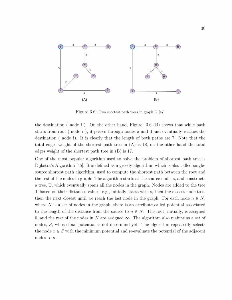
30

Figure 3.6: Two shortest path trees in graph G [47]

the destination ( node f ). On the other hand, Figure 3.6 (B) shows that while path

starts from root ( node r ), it passes through nodes a and d and eventually reaches the

destination ( node f). It is clearly that the length of both paths are 7. Note that the

total edges weight of the shortest path tree in (A) is 18, on the other hand the total

edges weight of the shortest path tree in (B) is 17.

One of the most popular algorithm used to solve the problem of shortest path tree is

Dijkstra’s Algorithm [45]. It is defined as a greedy algorithm, which is also called single-

source shortest path algorithm, used to compute the shortest path between the root and

the rest of the nodes in graph. The algorithm starts at the source node, s, and constructs

a tree, T, which eventually spans all the nodes in the graph. Nodes are added to the tree

T based on their distances values, e.g., initially starts with s, then the closest node to s,

then the next closest until we reach the last node in the graph. For each node n ∈ N ,

where N is a set of nodes in the graph, there is an attribute called potential associated

to the length of the distance from the source to n ∈ N . The root, initially, is assigned

0, and the rest of the nodes in N are assigned ∞. The algorithm also maintains a set of

nodes, S, whose final potential is not determind yet. The algorithm repeatedly selects

the node x ∈ S with the minimum potential and re-evaluate the potential of the adjacent

nodes to x.

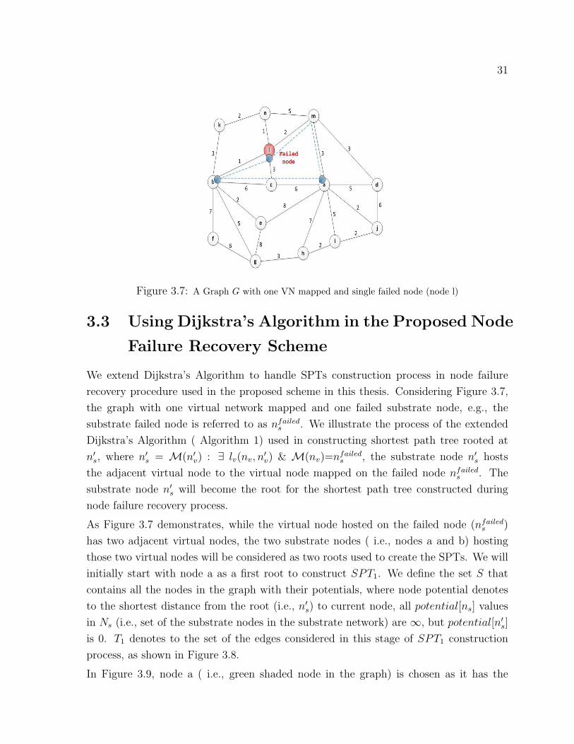
31

Figure 3.7: A Graph G with one VN mapped and single failed node (node l)

3.3 Using Dijkstra’s Algorithm in the Proposed Node

Failure Recovery Scheme

We extend Dijkstra’s Algorithm to handle SPTs construction process in node failure

recovery procedure used in the proposed scheme in this thesis. Considering Figure 3.7,

the graph with one virtual network mapped and one failed substrate node, e.g., the

substrate failed node is referred to as nfaileds . We illustrate the process of the extended

Dijkstra’s Algorithm ( Algorithm 1) used in constructing shortest path tree rooted at

n′s, where n′

s = M(n′v) : ∃ lv(nv, n

′v) & M(nv)=nfailed

s , the substrate node n′s hosts

the adjacent virtual node to the virtual node mapped on the failed node nfaileds . The

substrate node n′s will become the root for the shortest path tree constructed during

node failure recovery process.

As Figure 3.7 demonstrates, while the virtual node hosted on the failed node (nfaileds )

has two adjacent virtual nodes, the two substrate nodes ( i.e., nodes a and b) hosting

those two virtual nodes will be considered as two roots used to create the SPTs. We will

initially start with node a as a first root to construct SPT1. We define the set S that

contains all the nodes in the graph with their potentials, where node potential denotes

to the shortest distance from the root (i.e., n′s) to current node, all potential[ns] values

in Ns (i.e., set of the substrate nodes in the substrate network) are ∞, but potential[n′s]

is 0. T1 denotes to the set of the edges considered in this stage of SPT1 construction

process, as shown in Figure 3.8.

In Figure 3.9, node a ( i.e., green shaded node in the graph) is chosen as it has the

32

Algorithm 1 Dijkstra’s Algorithm used in the proposed scheme1: Input: A weighted and undirected graph Gs = (Ns, Ls, Rs), a weighted graph Gv =

(Nv, Lv), and a failed node nfaileds .

2: Output: A shortest-path tree SPT rooted at n′s, where n′

s= M(n′v) : ∃ lv(nv, n

′v) &

M(nv)=nfaileds .

3: for each node ns ∈ Ns do

4: potential[ns]←∞5: preceder[ns]← NIL

6: end for

7: potential[n′s]← 0

8: T ←ϕ

9: S ←Ns / nfaileds

10: while S ̸= ϕ do

11: Select x ∈ S with minimum potential[x]

12: S ← S/{x}13: if x ̸= n′

s then

14: T ← T ∪ {(preceder[x], x)}15: end if

16: for each node u adjacent to x do

17: if potential[u]>potential[x] + length(x, u) then

18: potential[u]← potential[x] + length(x, u)

19: preceder[u]← x

20: end if

21: end for

22: end while

33

Figure 3.8: The Graph G with the first root (node a)

Figure 3.9: Choosing the root in SPT1 construction

minimum potential value in S. All the edges incident to node a ( i.e., dotted edges in

the graph) are relaxed, and the adjacent nodes to root (node a) change their potential

values to the total of the potential value of the root plus the weight of the edges between

the root and its adjacents, Algorithm 1.

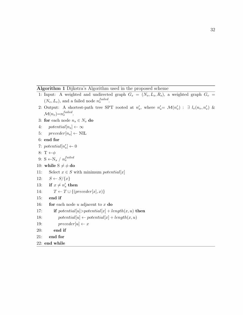
Node j is chosen from the graph in Figure 3.10 since its potential value is the minimum

and removed from S. The adjacent nodes d and i are re-evaluated based on the weight

of the edges and the potential value of node j. The edge (a,j) is added to SPT1 under

construction, this is referred as T1 = {(a, J)}.Now the marked node m in Figure 3.11 has the minimum potential value among all nodes

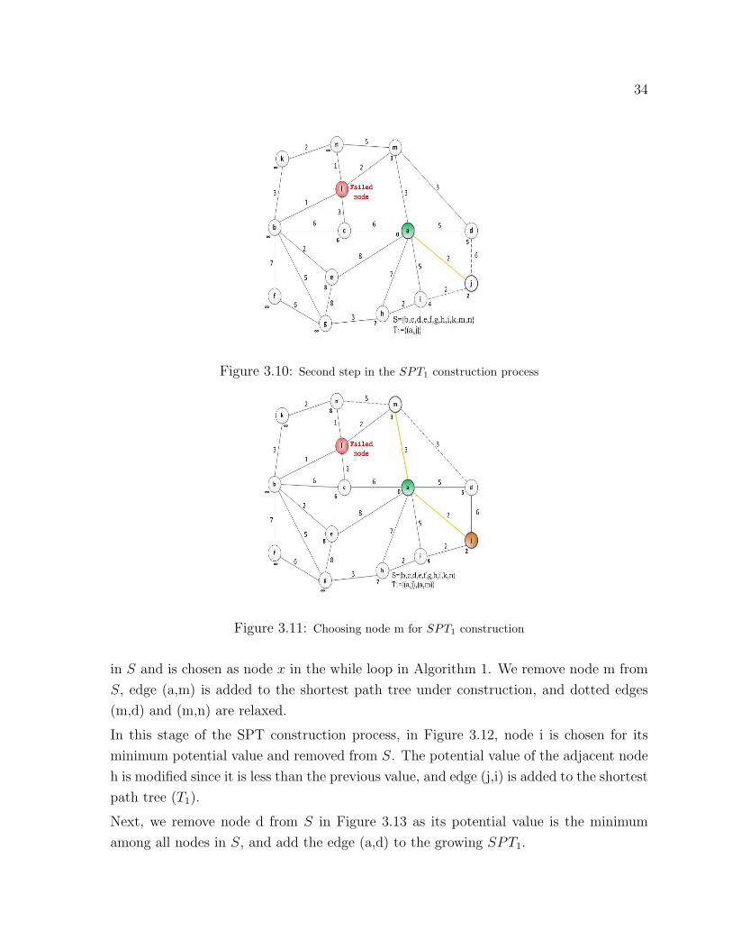
34

Figure 3.10: Second step in the SPT1 construction process

Figure 3.11: Choosing node m for SPT1 construction

in S and is chosen as node x in the while loop in Algorithm 1. We remove node m from

S, edge (a,m) is added to the shortest path tree under construction, and dotted edges

(m,d) and (m,n) are relaxed.

In this stage of the SPT construction process, in Figure 3.12, node i is chosen for its

minimum potential value and removed from S. The potential value of the adjacent node

h is modified since it is less than the previous value, and edge (j,i) is added to the shortest

path tree (T1).

Next, we remove node d from S in Figure 3.13 as its potential value is the minimum

among all nodes in S, and add the edge (a,d) to the growing SPT1.

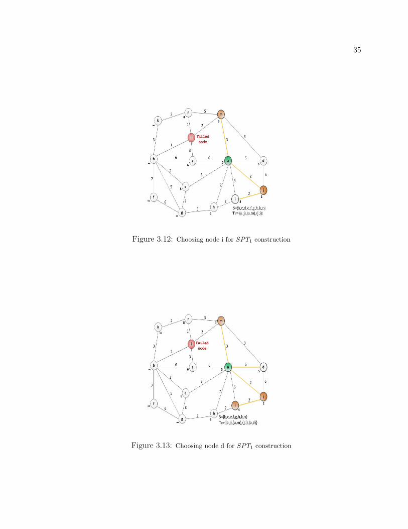
35

Figure 3.12: Choosing node i for SPT1 construction

Figure 3.13: Choosing node d for SPT1 construction

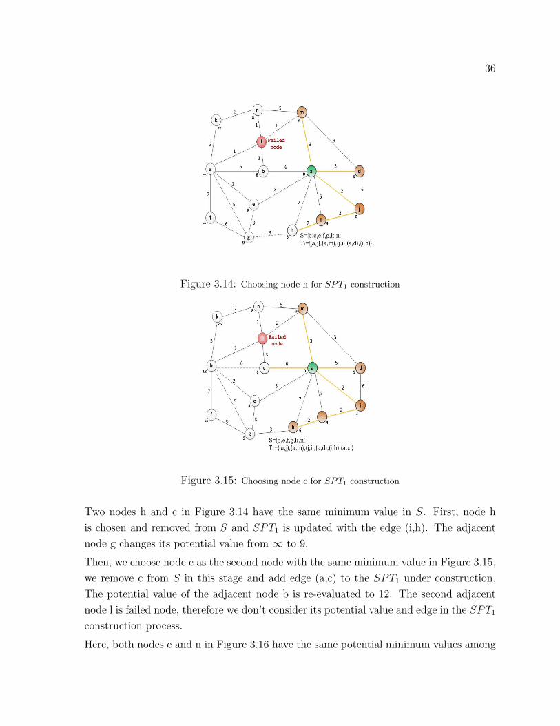
36

Figure 3.14: Choosing node h for SPT1 construction

Figure 3.15: Choosing node c for SPT1 construction

Two nodes h and c in Figure 3.14 have the same minimum value in S. First, node h

is chosen and removed from S and SPT1 is updated with the edge (i,h). The adjacent

node g changes its potential value from ∞ to 9.

Then, we choose node c as the second node with the same minimum value in Figure 3.15,

we remove c from S in this stage and add edge (a,c) to the SPT1 under construction.

The potential value of the adjacent node b is re-evaluated to 12. The second adjacent

node l is failed node, therefore we don’t consider its potential value and edge in the SPT1

construction process.

Here, both nodes e and n in Figure 3.16 have the same potential minimum values among

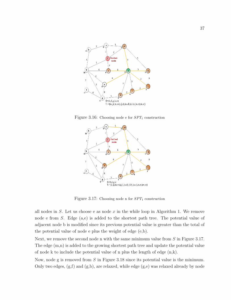
37

Figure 3.16: Choosing node e for SPT1 construction

Figure 3.17: Choosing node n for SPT1 construction

all nodes in S. Let us choose e as node x in the while loop in Algorithm 1. We remove

node e from S. Edge (a,e) is added to the shortest path tree. The potential value of

adjacent node b is modified since its previous potential value is greater than the total of

the potential value of node e plus the weight of edge (e,b).

Next, we remove the second node n with the same minimum value from S in Figure 3.17.

The edge (m,n) is added to the growing shortest path tree and update the potential value

of node k to include the potential value of n plus the length of edge (n,k).

Now, node g is removed from S in Figure 3.18 since its potential value is the minimum.

Only two edges, (g,f) and (g,b), are relaxed, while edge (g,e) was relaxed already by node

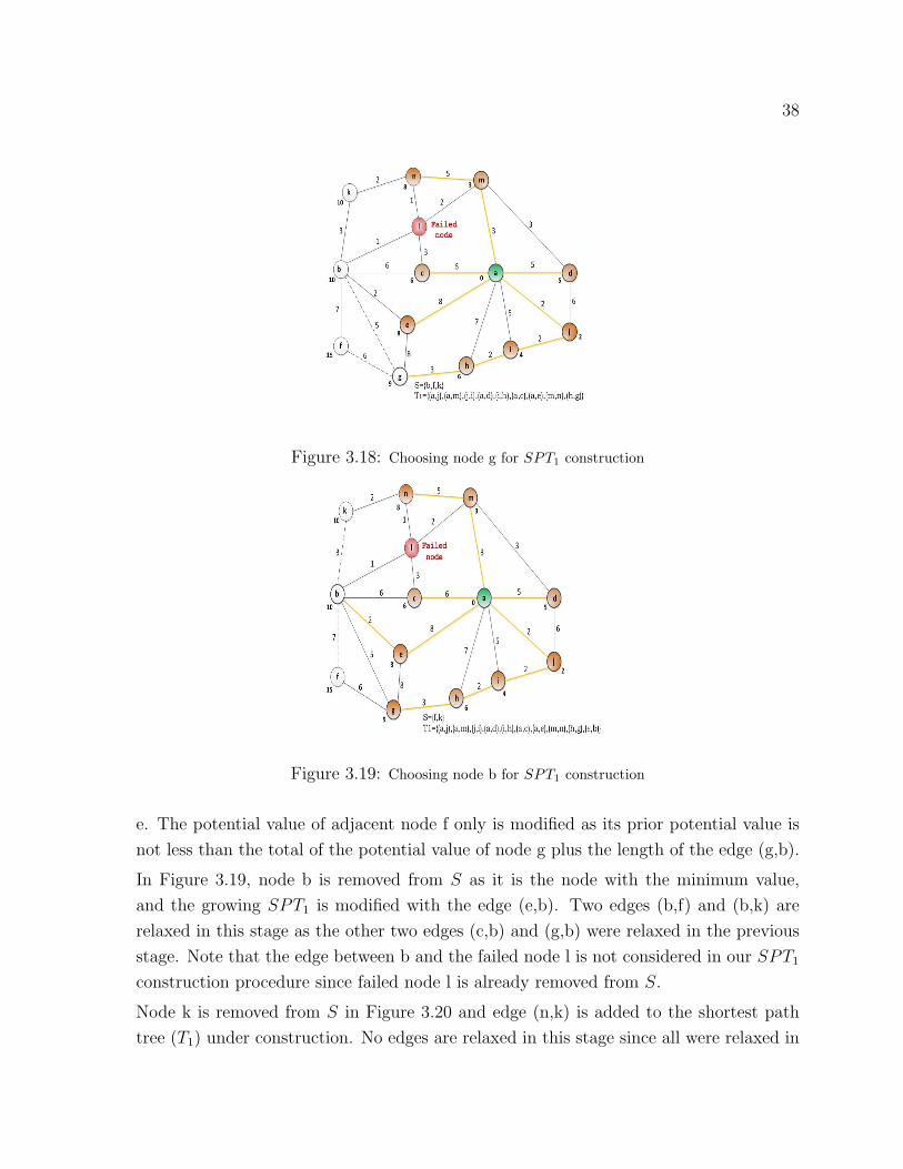
38

Figure 3.18: Choosing node g for SPT1 construction

Figure 3.19: Choosing node b for SPT1 construction

e. The potential value of adjacent node f only is modified as its prior potential value is

not less than the total of the potential value of node g plus the length of the edge (g,b).

In Figure 3.19, node b is removed from S as it is the node with the minimum value,

and the growing SPT1 is modified with the edge (e,b). Two edges (b,f) and (b,k) are

relaxed in this stage as the other two edges (c,b) and (g,b) were relaxed in the previous

stage. Note that the edge between b and the failed node l is not considered in our SPT1

construction procedure since failed node l is already removed from S.

Node k is removed from S in Figure 3.20 and edge (n,k) is added to the shortest path

tree (T1) under construction. No edges are relaxed in this stage since all were relaxed in

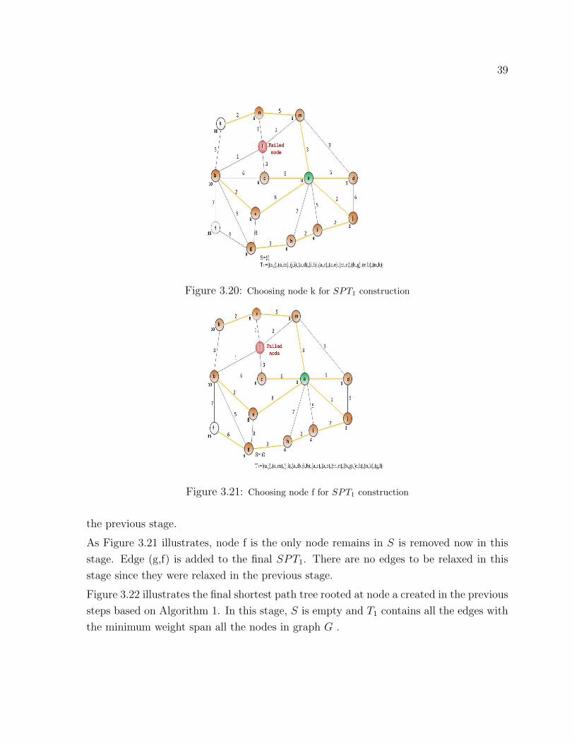
39

Figure 3.20: Choosing node k for SPT1 construction

Figure 3.21: Choosing node f for SPT1 construction

the previous stage.

As Figure 3.21 illustrates, node f is the only node remains in S is removed now in this

stage. Edge (g,f) is added to the final SPT1. There are no edges to be relaxed in this

stage since they were relaxed in the previous stage.

Figure 3.22 illustrates the final shortest path tree rooted at node a created in the previous

steps based on Algorithm 1. In this stage, S is empty and T1 contains all the edges with

the minimum weight span all the nodes in graph G .

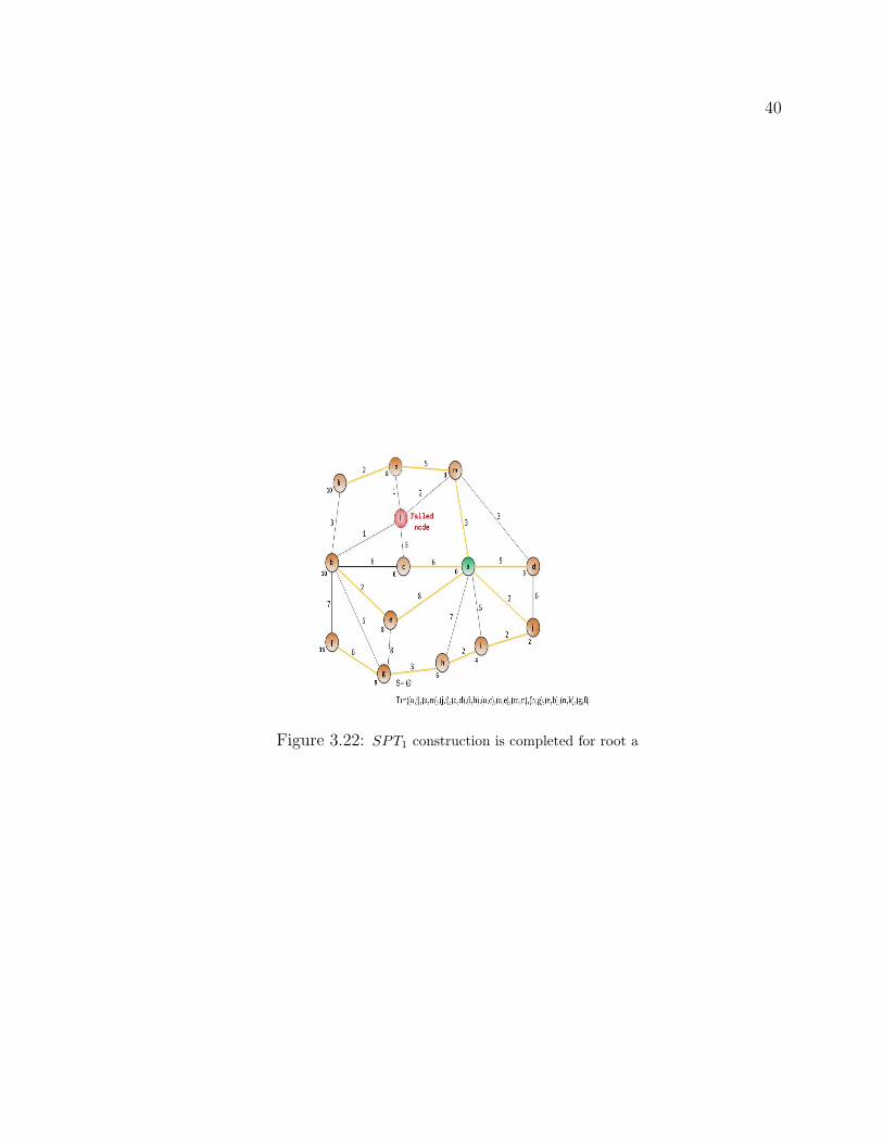
40

Figure 3.22: SPT1 construction is completed for root a

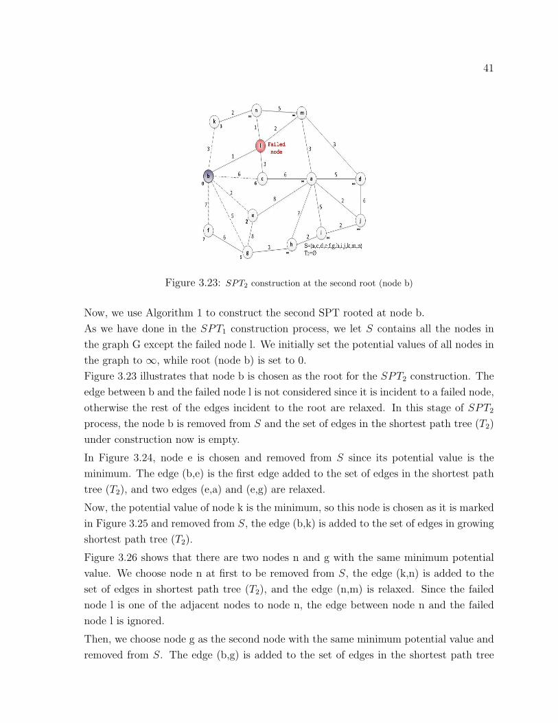
41

Figure 3.23: SPT2 construction at the second root (node b)

Now, we use Algorithm 1 to construct the second SPT rooted at node b.

As we have done in the SPT1 construction process, we let S contains all the nodes in

the graph G except the failed node l. We initially set the potential values of all nodes in

the graph to ∞, while root (node b) is set to 0.

Figure 3.23 illustrates that node b is chosen as the root for the SPT2 construction. The

edge between b and the failed node l is not considered since it is incident to a failed node,

otherwise the rest of the edges incident to the root are relaxed. In this stage of SPT2

process, the node b is removed from S and the set of edges in the shortest path tree (T2)

under construction now is empty.

In Figure 3.24, node e is chosen and removed from S since its potential value is the

minimum. The edge (b,e) is the first edge added to the set of edges in the shortest path

tree (T2), and two edges (e,a) and (e,g) are relaxed.

Now, the potential value of node k is the minimum, so this node is chosen as it is marked

in Figure 3.25 and removed from S, the edge (b,k) is added to the set of edges in growing

shortest path tree (T2).

Figure 3.26 shows that there are two nodes n and g with the same minimum potential

value. We choose node n at first to be removed from S, the edge (k,n) is added to the

set of edges in shortest path tree (T2), and the edge (n,m) is relaxed. Since the failed

node l is one of the adjacent nodes to node n, the edge between node n and the failed

node l is ignored.

Then, we choose node g as the second node with the same minimum potential value and

removed from S. The edge (b,g) is added to the set of edges in the shortest path tree

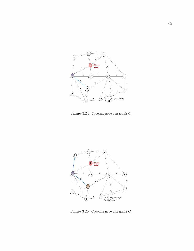
42

Figure 3.24: Choosing node e in graph G

Figure 3.25: Choosing node k in graph G

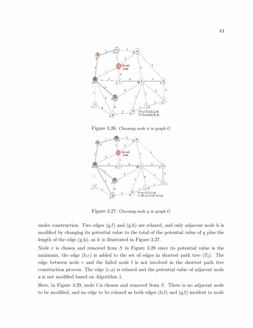
43

Figure 3.26: Choosing node n in graph G

Figure 3.27: Choosing node g in graph G

under construction. Two edges (g,f) and (g,h) are relaxed, and only adjacent node h is

modified by changing its potential value to the total of the potential value of g plus the

length of the edge (g,h), as it is illustrated in Figure 3.27.

Node c is chosen and removed from S in Figure 3.28 since its potential value is the

minimum, the edge (b,c) is added to the set of edges in shortest path tree (T2). The

edge between node c and the failed node l is not involved in the shortest path tree

construction process. The edge (c,a) is relaxed and the potential value of adjacent node

a is not modified based on Algorithm 1.

Here, in Figure 3.29, node f is chosen and removed from S. There is no adjacent node

to be modified, and no edge to be relaxed as both edges (b,f) and (g,f) incident to node

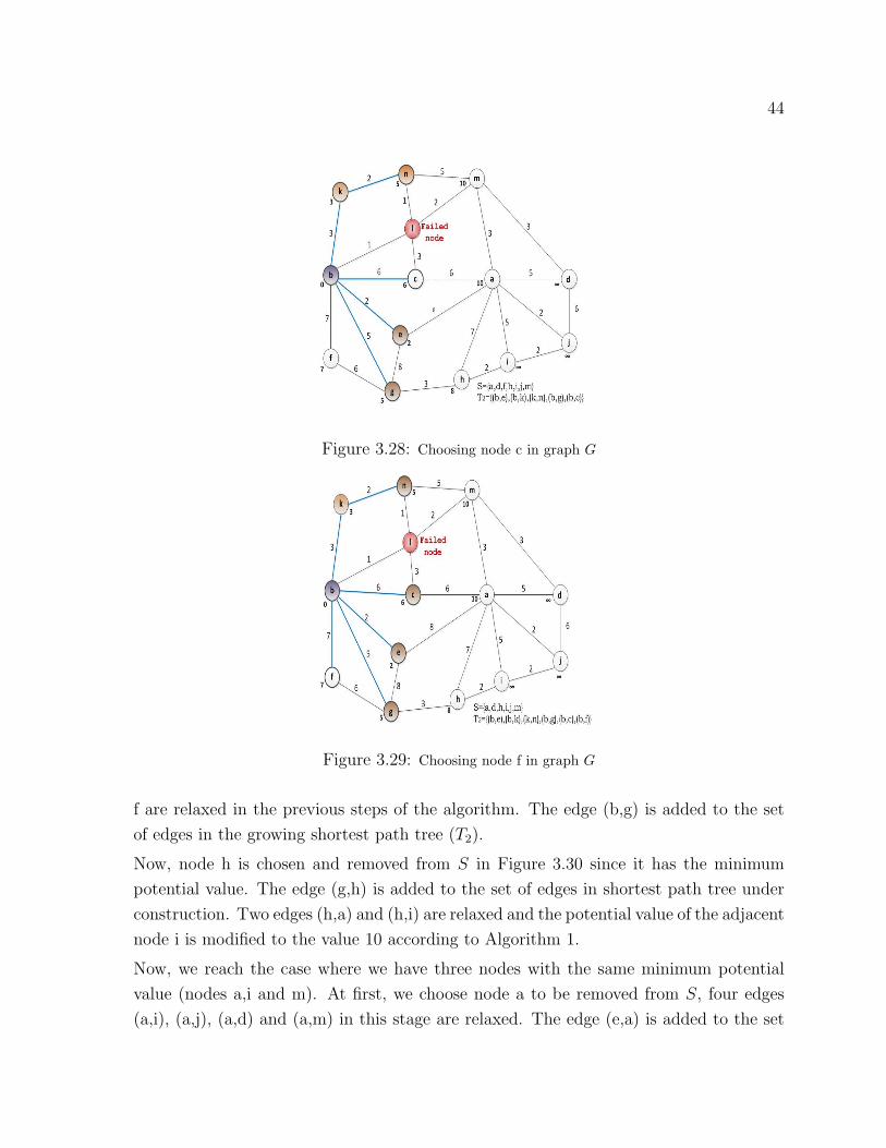
44

Figure 3.28: Choosing node c in graph G

Figure 3.29: Choosing node f in graph G

f are relaxed in the previous steps of the algorithm. The edge (b,g) is added to the set

of edges in the growing shortest path tree (T2).

Now, node h is chosen and removed from S in Figure 3.30 since it has the minimum

potential value. The edge (g,h) is added to the set of edges in shortest path tree under

construction. Two edges (h,a) and (h,i) are relaxed and the potential value of the adjacent

node i is modified to the value 10 according to Algorithm 1.

Now, we reach the case where we have three nodes with the same minimum potential

value (nodes a,i and m). At first, we choose node a to be removed from S, four edges

(a,i), (a,j), (a,d) and (a,m) in this stage are relaxed. The edge (e,a) is added to the set

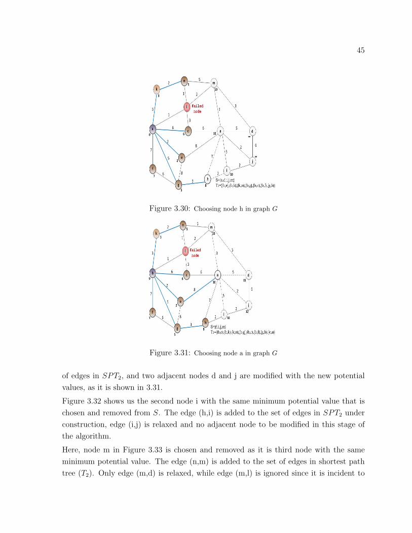
45

Figure 3.30: Choosing node h in graph G

Figure 3.31: Choosing node a in graph G

of edges in SPT2, and two adjacent nodes d and j are modified with the new potential

values, as it is shown in 3.31.

Figure 3.32 shows us the second node i with the same minimum potential value that is

chosen and removed from S. The edge (h,i) is added to the set of edges in SPT2 under

construction, edge (i,j) is relaxed and no adjacent node to be modified in this stage of

the algorithm.

Here, node m in Figure 3.33 is chosen and removed as it is third node with the same

minimum potential value. The edge (n,m) is added to the set of edges in shortest path

tree (T2). Only edge (m,d) is relaxed, while edge (m,l) is ignored since it is incident to

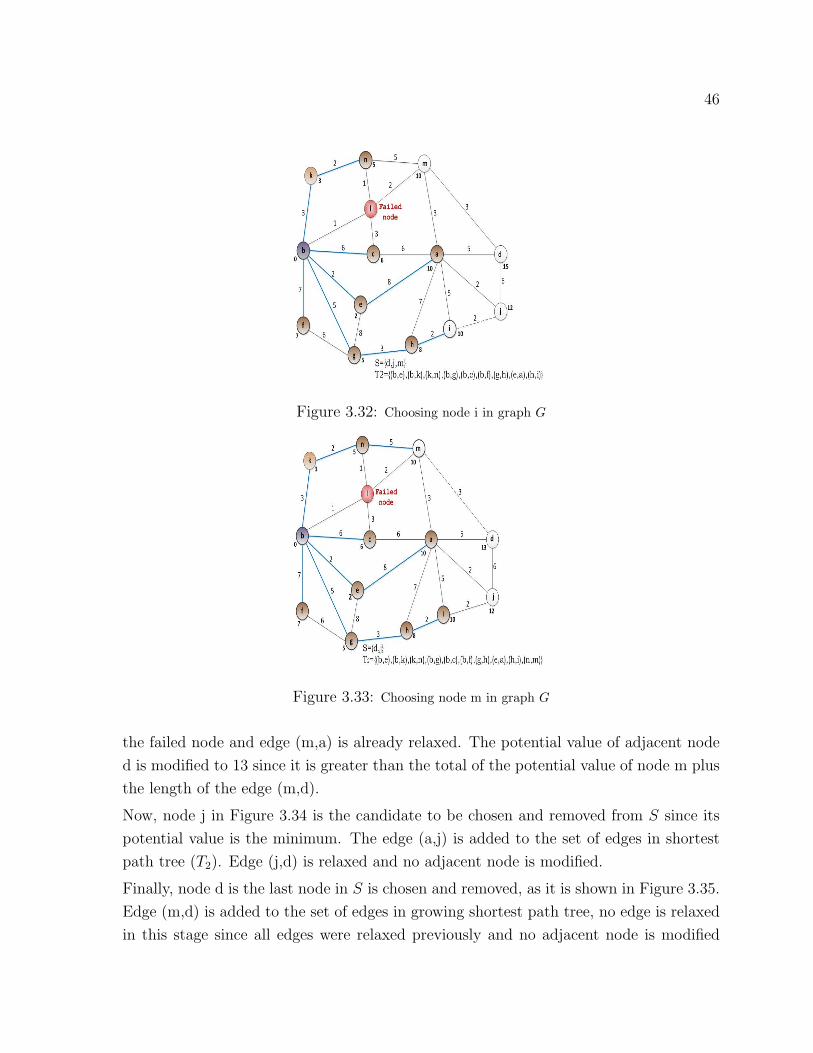
46

Figure 3.32: Choosing node i in graph G

Figure 3.33: Choosing node m in graph G

the failed node and edge (m,a) is already relaxed. The potential value of adjacent node

d is modified to 13 since it is greater than the total of the potential value of node m plus

the length of the edge (m,d).

Now, node j in Figure 3.34 is the candidate to be chosen and removed from S since its

potential value is the minimum. The edge (a,j) is added to the set of edges in shortest

path tree (T2). Edge (j,d) is relaxed and no adjacent node is modified.

Finally, node d is the last node in S is chosen and removed, as it is shown in Figure 3.35.

Edge (m,d) is added to the set of edges in growing shortest path tree, no edge is relaxed

in this stage since all edges were relaxed previously and no adjacent node is modified

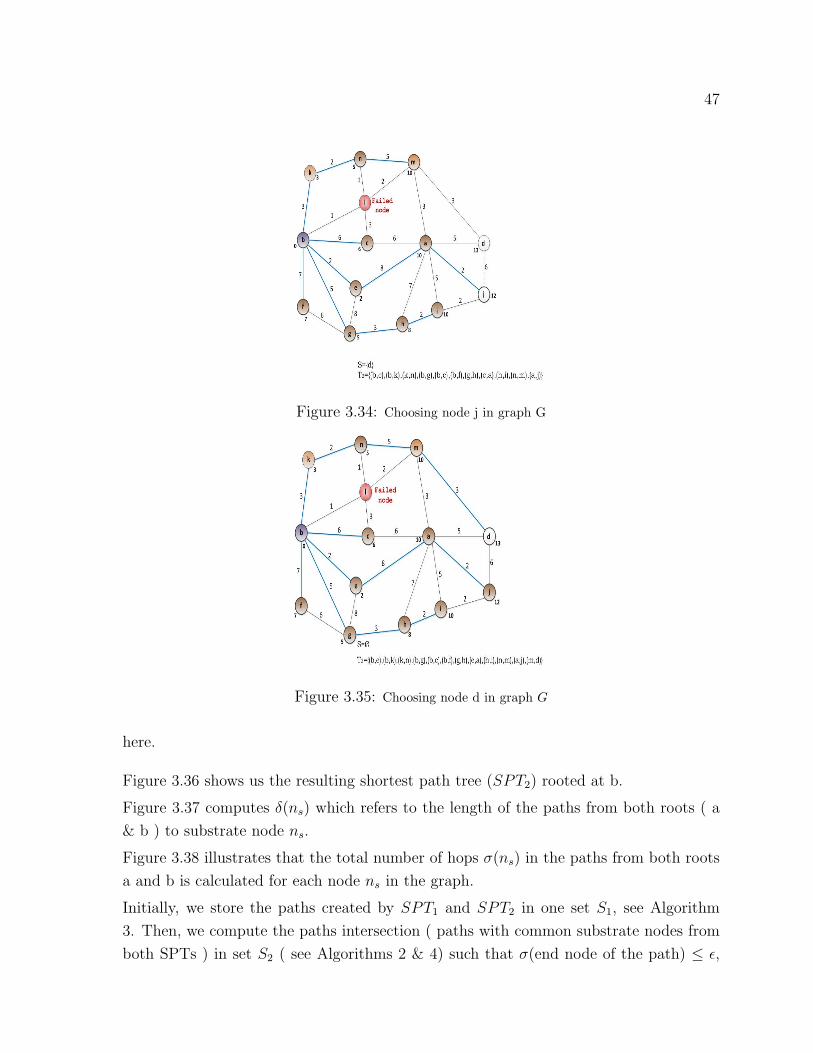
47

Figure 3.34: Choosing node j in graph G

Figure 3.35: Choosing node d in graph G

here.

Figure 3.36 shows us the resulting shortest path tree (SPT2) rooted at b.

Figure 3.37 computes δ(ns) which refers to the length of the paths from both roots ( a

& b ) to substrate node ns.

Figure 3.38 illustrates that the total number of hops σ(ns) in the paths from both roots

a and b is calculated for each node ns in the graph.

Initially, we store the paths created by SPT1 and SPT2 in one set S1, see Algorithm

3. Then, we compute the paths intersection ( paths with common substrate nodes from

both SPTs ) in set S2 ( see Algorithms 2 & 4) such that σ(end node of the path) ≤ ϵ,

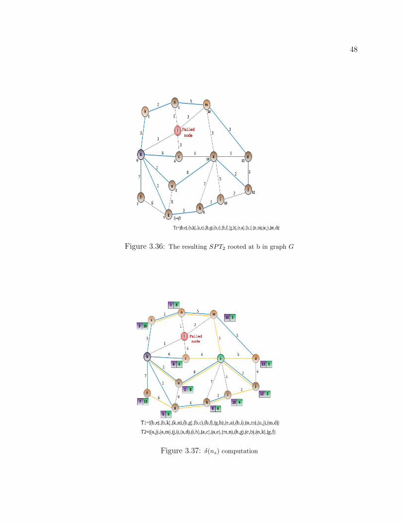
48

Figure 3.36: The resulting SPT2 rooted at b in graph G

Figure 3.37: δ(ns) computation

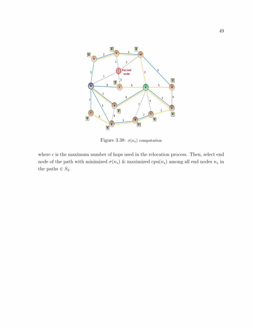
49

Figure 3.38: σ(ns) computation

where ϵ is the maximum number of hops used in the relocation process. Then, select end

node of the path with minimized σ(ns) & maximized cpu(ns) among all end nodes ns in

the paths ∈ S2.

50

3.4 Proposed Recovery Algorithm

The process of relocating the VN nodes hosted on the failed node nfaileds is triggered

when the InP sends a recovery request to the corresponding manager node (e.g., node

9 in Figure 3.1). The recovery process for each affected VN node proceeds as follows:

the manager node forwards the recovery request to all SN nodes hosting virtual nodes

adjacent to affected VN nodes (e.g., node 1 and node 4 in Figure 3.1). Each of these

nodes construct a shortest path tree (SPT) to all SN nodes at a distance at most ϵ 1 hops

from the node with the root of the SPT representing the node itself ( i.e., Figure 3.38).

The manager node employs these paths to select the node with the shortest distance to

all the SN nodes that are hosting VN nodes adjacent to that on the failed node. This

node eventually becomes the optimal candidate node to host the affected VN node. The

length of the resulting paths from SPT must be less than or equal to ϵ, the maximum

number of hops allowed for a path that maps a VN link. Also, the capacity of the end

nodes 2 of the paths must be greater than or equal to the capacity of the virtual node

hosted on the failed node (e.g., node b). The manager node selects the optimal candidate

node by computing the intersection of the paths resulted from running SPT algorithm

for all SN nodes hosting neighbour VN nodes of the affected node in failed node. The

paths with minimum length and end nodes of the paths with maximum capacity are

selected. Figure 3.2 depicts the graph resulting from executing the node failure recovery

algorithm. Algorithm 2 provides a peseudo code description of node failure recovery.

3.5 Node Failure Recovery for Overloaded Networks

In the overloaded substrate network, the probability of failing to find a new optimal

candidate node for the VN nodes hosted on the failed node will be high. There are

two possible causes of this event: overloaded substrate nodes and bottleneck substrate

links. To operate the node failure recovery algorithm in the overloaded network, a

reconfiguration procedure is first executed to migrate one or more virtual nodes hosted

on the overloaded substrate nodes to free up some cpu capacity in the substrate node

or some bandwidth in the SN links to be able to relocate the hosted VN node in failed

node.

1The threshold for the max number of links is decided by the SP.2The term end node is used to refer to the last node in the path.

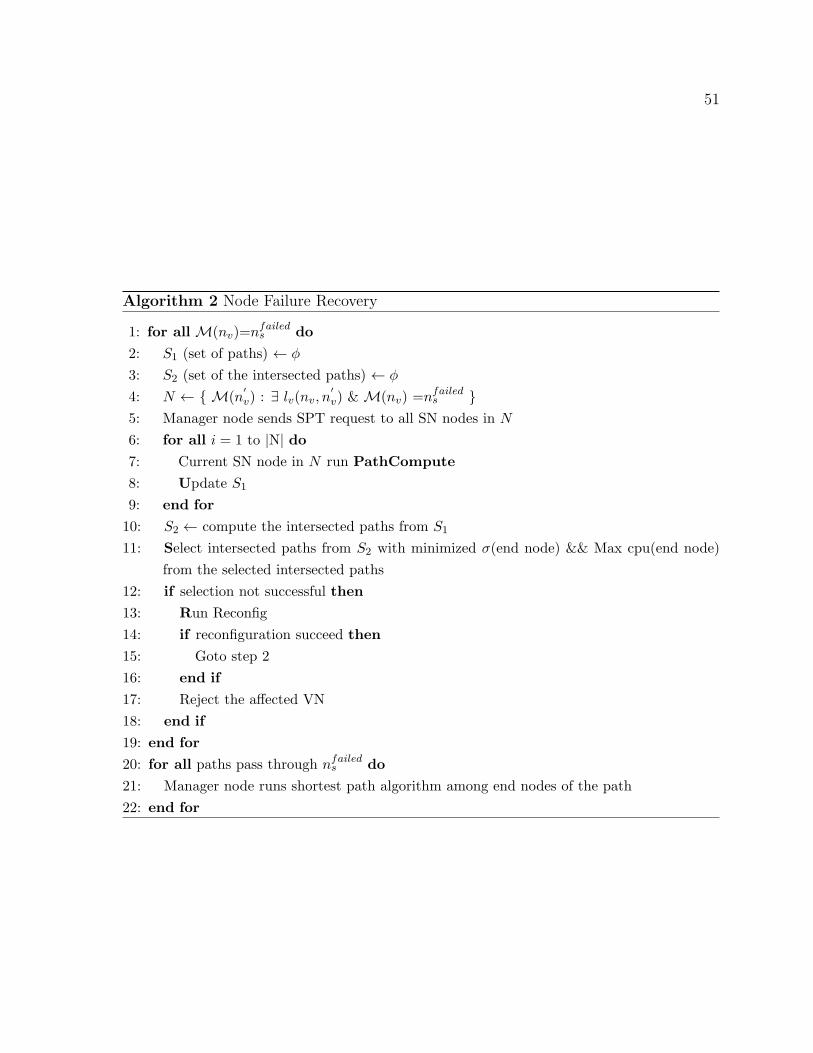
51

Algorithm 2 Node Failure Recovery

1: for allM(nv)=nfaileds do

2: S1 (set of paths) ← ϕ

3: S2 (set of the intersected paths) ← ϕ

4: N ← { M(n′v) : ∃ lv(nv, n

′v) &M(nv) =nfailed

s }5: Manager node sends SPT request to all SN nodes in N

6: for all i = 1 to |N| do7: Current SN node in N run PathCompute

8: Update S1

9: end for

10: S2 ← compute the intersected paths from S1

11: Select intersected paths from S2 with minimized σ(end node) && Max cpu(end node)

from the selected intersected paths

12: if selection not successful then

13: Run Reconfig

14: if reconfiguration succeed then

15: Goto step 2

16: end if

17: Reject the affected VN

18: end if

19: end for

20: for all paths pass through nfaileds do

21: Manager node runs shortest path algorithm among end nodes of the path

22: end for

52

3.5.1 Insufficient CPU Capacity of the Nodes Hosting SPTs

Nodes

The process of reconfiguration starts by sorting all the virtual nodes hosted on the SPT

nodes. The criteria ( CRT , in line 1 in Algorithm 4) used for sorting these VN nodes

are: the residual CPU capacity of the nodes hosting these VN nodes and the life time of

the VNs containing these VN nodes. Then, the recovery procedure is executed on the

first sorted VN node that carries the highest CPU capacity to be relocated to a new SN

node. If the migration of the virtual node succeeds in releasing enough capacity, then

the node failure recovery mechanism is executed again to relocate the affected VN node

in the failed node. Otherwise, the above procedure is repeated on the rest of the sorted

list of virtual nodes until affected VN node relocation succeeds, (see Algorithm 4).

3.5.2 SPTs Traverse Bottleneck SN Links

When the constructed SPTs pass through bottleneck substrate link or links, a virtual

link on a bottleneck SN link is relocated to release enough bandwidth to be used again

in node failure recovery. First, all the VN nodes hosted on the SPTs nodes are sorted

according to the following criteria (CRT, line 1 in Algorithm 4): the life time of the VN

where virtual nodes belong to and the number of the overloaded SN links where SPTs

pass through. Next, the recovery procedure is excuted to migrate the first sorted virtual

node. If it fails to release enough bandwidth, the recovery procedure is executed on the

next sorted VN node. The execution of recovery procedure is repeated on the rest of

the listed VN nodes untill enough bandwidth become available to relocate the affected

virtual node on the failed node. After enough bandwidth is released in the overloaded

links, node failure recovery algorithm is executed to relocate the affected virtual node on

the failed SN node, (see Algorithm 4).

The procedure in Algorithm 3 computes the SPTs that are deployed to generate the set

of intersected paths for all the neighbours of the affected VN node in the failed SN node,

this procedure is used in Algorithms 2 and 4.

The failed SN node may not only be hosting some virtual nodes, but some paths from

different VNs might also traverse it. Node failure recovery approach runs the shortest

path algorithm over the end nodes of those paths to relocate them to pass through any

node other than failed node. To get a new SN path, the manager node sends a shortest

path request to any end node of the SN path hosting the VN link need to be relocated.

53

Algorithm 3 PathCompute1: Run Algorithm 1 to compute SPT between current SN node in N and all nodes in SN not

hosting virtual node used by VN using the virtual node need to be relocated

2: pSet← Store the resulting paths from running Algorithm 1

3: for all paths ∈ pSet do

4: if σ(end node of current path)≤ ϵ && cpu(end node)≥ cpu capacity of the virtual node

need to be relocated then

5: S1 ← Add current path

6: end if

7: end for

Next, the SN node executes the shortest path algorithm to the other end node of the

path, and when creating a new path, the manager node reallocates the virtual link to

this new SN path.

3.6 Time Complexity Analysis of the Proposed Al-

gorithm

In this section we compute the time complexity of the proposed node failure recovery

algorithm to relocate one virual node from the failed node. Note that, the major tasks of

proposed node failure recovery algorithm (Algorithm 2) can be classified into two types:

• Task one: constructing the shortest path tree.

• Task two: computing the paths intersection.

We extend Disjkstra’s algorithm to construct the shortest path trees to the SN nodes

with the root of neighbours (task one). Since Algorithm 1 (Disjkstra’s algorithm) has

two main loops, the time complexity of shortest path tree construction algorithm with

single source is computed as the following:

T (n) = (n− 1)2 ∈ θ(n2) (3.5)

Equation 3.5 illustrates that Disjkstra’s algorithm is executed in polynomial time. How-

ever, it is possible that Disjkstra’s algorithm be implemented using a heap or Fibonacci

heap [46]. The time complexity of using heap implementation is θ(m lgn), and of using

Fibonacci heap implementation is θ(m + n lgn), where m is the number of edges.

54

Algorithm 4 Reconfig1: z ← Sort out all the virtual nodes decreasingly, those virtual nodes are hosted on the nodes

over which intersected paths traverse, sorting is based on the criteria CRT

2: Set done = false

3: while done ̸= true & z ̸= ϕ do

4: S1 (set of paths) ← ϕ

5: S2 (set of the intersected paths) ← ϕ

6: N ← { M(n′v) : ∃ lv(nv,n

′v), nv= current nv in z }

7: for all i = 1 to |N| do8: Current SN node in N run PathCompute

9: Update S1

10: end for

11: S2 ← compute the intersected paths from S1

12: Select intersected paths with minimized σ(end node) from S2 && end node with max

capacity from the selected intersected paths

13: if selection succeed then

14: done=true

15: end if

16: end while

55

Algorithm 2 illustrates that the number of times to execute Algorithm 1 ( SPT con-

struction ) depends on the count of the neighbours of the VN node hosted on the failed

node. Thus, if we assume that the number of neighbours is c, then the time complexity

of executing the shortest path tree algorithm in c times is the same as the following:

T (n) = θ(n2) (3.6)

In the second major task of Algorithm 2, the intersected paths are computed from the set

of the paths created by Algorithm 1 (Disjkstra’s algorithm). To compute the intersected

paths we need two loops to compare between paths, and the worst case is when we

construct a shortest path tree to all nodes in the tree which means n − 2. Thus, the

time complexiy of the paths intersection is computed as the following:

T (n) = (n− 2)2 ∈ θ(n2) (3.7)

Based on the equations in 3.6 and 3.7, we compute the final time complexity of the

proposed node failure recovery algorithm which can be executed in polynomial time as

following:

T (n) = max[θ(n2), θ(n2)] ∈ θ(n2) (3.8)

Chapter 4

Performance Evaluation

In this section, we first describe the simulation environment in which we evaluate our

approach, and then we present the evaluation results. The main focus of our evaluation

is to demonstrate the benefits of the proposed approach in reducing the node failure

recovery cost and service intrruption time over Star-shaped VN component migration

scheme [11] in the event of node failure.

4.1 Simulation Environment

We have extended the implementation of the discrete event simulator ”ViNE-Yard” [49]

to evaluate the performance of the proposed node failure recovery approach, and to

demonstrate the advantages of utilizing node failure recovery scheme in a decentralized

manner against Star-shaped VN component migration scheme [11]. The GT-ITM tool

[50] is used to generate the random substrate network and the VN requests.

Following previous work [8] [6] [13], we adopt the following simulation scenario: the SN

topologies used in our experiments are set to 50 nodes. Each pair of nodes is randomly

connected with probability 0.5. The CPU of the substrate nodes and the bandwidth

of the links are real numbers uniformly distributed between 50 and 100. The CPU

requirements of the nodes on the VN are real numbers uniformly distributed between

0 to 20 and the bandwidth requirements of the virtual links are uniformly distributed

between 0 to 50. In the VN requests, the number of nodes is randomly determined by a

uniform distribution between 2 and 15. Following [9], we assume that the VN requests

and substrate node failure events follow a Poisson process with arrival rates λV and λF

respectively. We assume that λV is 4 events per 100 time units. The VN lifetime is

56

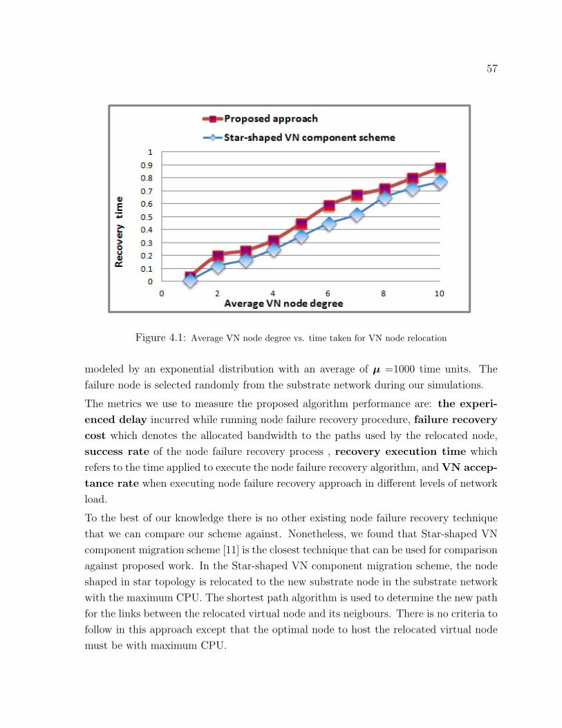
57

Figure 4.1: Average VN node degree vs. time taken for VN node relocation

modeled by an exponential distribution with an average of µ =1000 time units. The

failure node is selected randomly from the substrate network during our simulations.

The metrics we use to measure the proposed algorithm performance are: the experi-

enced delay incurred while running node failure recovery procedure, failure recovery

cost which denotes the allocated bandwidth to the paths used by the relocated node,

success rate of the node failure recovery process , recovery execution time which

refers to the time applied to execute the node failure recovery algorithm, andVN accep-

tance rate when executing node failure recovery approach in different levels of network

load.

To the best of our knowledge there is no other existing node failure recovery technique

that we can compare our scheme against. Nonetheless, we found that Star-shaped VN

component migration scheme [11] is the closest technique that can be used for comparison

against proposed work. In the Star-shaped VN component migration scheme, the node

shaped in star topology is relocated to the new substrate node in the substrate network

with the maximum CPU. The shortest path algorithm is used to determine the new path

for the links between the relocated virtual node and its neigbours. There is no criteria to

follow in this approach except that the optimal node to host the relocated virtual node

must be with maximum CPU.

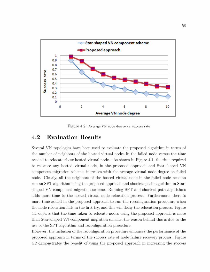
58

Figure 4.2: Average VN node degree vs. success rate

4.2 Evaluation Results

Several VN topologies have been used to evaluate the proposed algorithm in terms of

the number of neighbors of the hosted virtual nodes in the failed node versus the time

needed to relocate those hosted virtual nodes. As shown in Figure 4.1, the time required

to relocate any hosted virtual node, in the proposed approach and Star-shaped VN

component migration scheme, increases with the average virtual node degree on failed

node. Clearly, all the neighbors of the hosted virtual node in the failed node need to

run an SPT algorithm using the proposed approach and shortest path algorithm in Star-

shaped VN component migration scheme. Running SPT and shortest path algorithms

adds more time to the hosted virtual node relocation process. Furthermore, there is

more time added in the proposed approach to run the reconfiguration procedure when

the node relocation fails in the first try, and this will delay the relocation process. Figure

4.1 depicts that the time taken to relocate nodes using the proposed approach is more

than Star-shaped VN component migration scheme, the reason behind this is due to the

use of the SPT algorithm and reconfiguration procedure.

However, the inclusion of the reconfiguration procedure enhances the performance of the

proposed approach in terms of the success rate of node failure recovery process. Figure

4.2 demonstrates the benefit of using the proposed approach in increasing the success

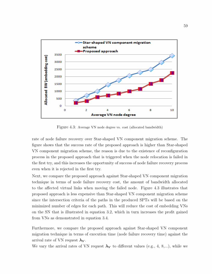
59

Figure 4.3: Average VN node degree vs. cost (allocated bandwidth)

rate of node failure recovery over Star-shaped VN component migration scheme. The

figure shows that the success rate of the proposed approach is higher than Star-shaped

VN component migration scheme, the reason is due to the existence of reconfiguration

process in the proposed approach that is triggered when the node relocation is failed in

the first try, and this increases the opportunity of success of node failure recovery process

even when it is rejected in the first try.

Next, we compare the proposed approach against Star-shaped VN component migration

technique in terms of node failure recovery cost, the amount of bandwidth allocated

to the affected virtual links when moving the failed node. Figure 4.3 illustrates that

proposed approach is less expensive than Star-shaped VN component migration scheme

since the intersection criteria of the paths in the produced SPTs will be based on the

minimized number of edges for each path. This will reduce the cost of embedding VNs

on the SN that is illustrated in equation 3.2, which in turn increases the profit gained

from VNs as demonstrated in equation 3.4.

Furthermore, we compare the proposed approach against Star-shaped VN component

migration technique in terms of execution time (node failure recovery time) against the

arrival rate of VN request λV .

We vary the arrival rates of VN request λV to different values (e.g., 4, 8,...), while we

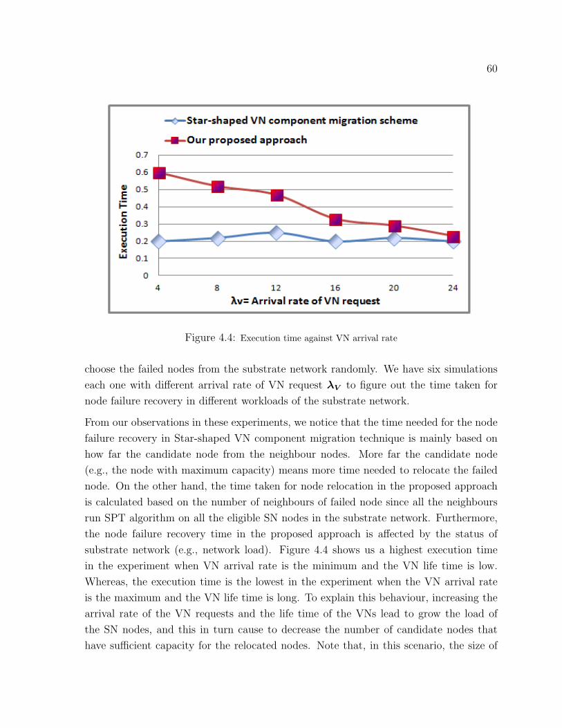
60

Figure 4.4: Execution time against VN arrival rate

choose the failed nodes from the substrate network randomly. We have six simulations

each one with different arrival rate of VN request λV to figure out the time taken for

node failure recovery in different workloads of the substrate network.

From our observations in these experiments, we notice that the time needed for the node

failure recovery in Star-shaped VN component migration technique is mainly based on

how far the candidate node from the neighbour nodes. More far the candidate node

(e.g., the node with maximum capacity) means more time needed to relocate the failed

node. On the other hand, the time taken for node relocation in the proposed approach

is calculated based on the number of neighbours of failed node since all the neighbours

run SPT algorithm on all the eligible SN nodes in the substrate network. Furthermore,

the node failure recovery time in the proposed approach is affected by the status of

substrate network (e.g., network load). Figure 4.4 shows us a highest execution time

in the experiment when VN arrival rate is the minimum and the VN life time is low.

Whereas, the execution time is the lowest in the experiment when the VN arrival rate

is the maximum and the VN life time is long. To explain this behaviour, increasing the

arrival rate of the VN requests and the life time of the VNs lead to grow the load of

the SN nodes, and this in turn cause to decrease the number of candidate nodes that

have sufficient capacity for the relocated nodes. Note that, in this scenario, the size of

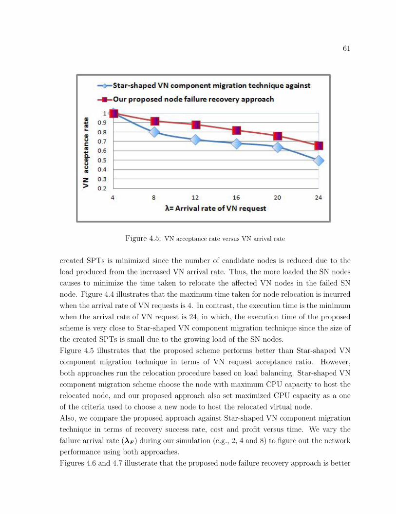
61

Figure 4.5: VN acceptance rate versus VN arrival rate

created SPTs is minimized since the number of candidate nodes is reduced due to the

load produced from the increased VN arrival rate. Thus, the more loaded the SN nodes

causes to minimize the time taken to relocate the affected VN nodes in the failed SN

node. Figure 4.4 illustrates that the maximum time taken for node relocation is incurred

when the arrival rate of VN requests is 4. In contrast, the execution time is the minimum

when the arrival rate of VN request is 24, in which, the execution time of the proposed

scheme is very close to Star-shaped VN component migration technique since the size of

the created SPTs is small due to the growing load of the SN nodes.

Figure 4.5 illustrates that the proposed scheme performs better than Star-shaped VN

component migration technique in terms of VN request acceptance ratio. However,

both approaches run the relocation procedure based on load balancing. Star-shaped VN

component migration scheme choose the node with maximum CPU capacity to host the

relocated node, and our proposed approach also set maximized CPU capacity as a one

of the criteria used to choose a new node to host the relocated virtual node.

Also, we compare the proposed approach against Star-shaped VN component migration

technique in terms of recovery success rate, cost and profit versus time. We vary the

failure arrival rate (λF ) during our simulation (e.g., 2, 4 and 8) to figure out the network

performance using both approaches.

Figures 4.6 and 4.7 illusterate that the proposed node failure recovery approach is better

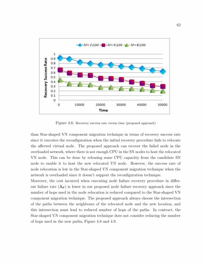
62

Figure 4.6: Recovery success rate versus time (proposed approach)

than Star-shaped VN component migration technique in terms of recovery success rate

since it executes the reconfiguration when the initial recovery procedure fails to relocate

the affected virtual node. The proposed approach can recover the failed node in the

overloaded network, where there is not enough CPU in the SN nodes to host the relocated

VN node. This can be done by releasing some CPU capacitiy from the candidate SN

node to enable it to host the new relocated VN node. However, the success rate of

node relocation is low in the Star-shaped VN component migration technique when the

network is overloaded since it doesn’t support the reconfiguration technique.

Moreover, the cost incurred when executing node failure recovery procedure in differ-

ent failure rate (λF ) is lower in our proposed node failure recovery approach since the

number of hops used in the node relocation is reduced compared to the Star-shaped VN

component migration technique. The proposed approach always choose the intersection

of the paths between the neighbours of the relocated node and the new location, and

this intersection must lead to reduced number of hops of the paths. In contract, the

Star-shaped VN component migration technique does not consider reducing the number

of hops used in the new paths, Figure 4.8 and 4.9.

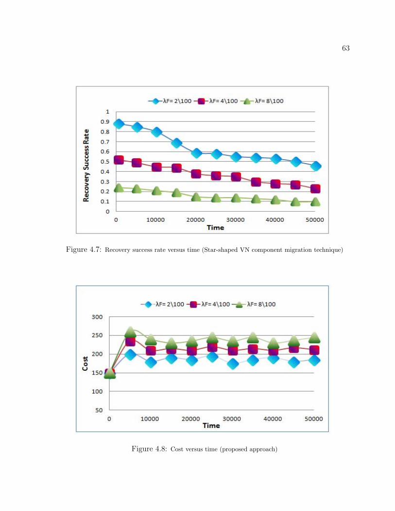
63

Figure 4.7: Recovery success rate versus time (Star-shaped VN component migration technique)

Figure 4.8: Cost versus time (proposed approach)

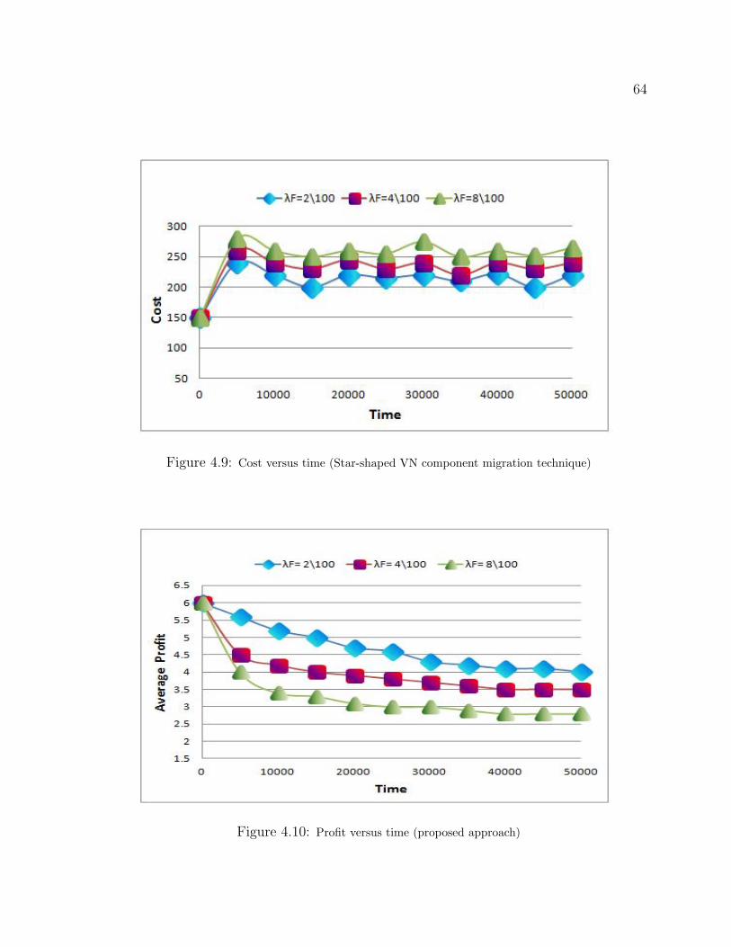
64

Figure 4.9: Cost versus time (Star-shaped VN component migration technique)

Figure 4.10: Profit versus time (proposed approach)

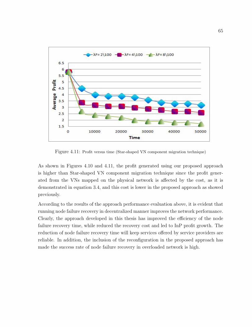
65

Figure 4.11: Profit versus time (Star-shaped VN component migration technique)

As shown in Figures 4.10 and 4.11, the profit generated using our proposed approach

is higher than Star-shaped VN component migration technique since the profit gener-

ated from the VNs mapped on the physical network is affected by the cost, as it is

demonstrated in equation 3.4, and this cost is lower in the proposed approach as showed

previously.

According to the results of the approach performance evaluation above, it is evident that

running node failure recovery in decentralized manner improves the network performance.

Clearly, the approach developed in this thesis has improved the efficiency of the node

failure recovery time, while reduced the recovery cost and led to InP profit growth. The

reduction of node failure recovery time will keep services offered by service providers are

reliable. In addition, the inclusion of the reconfiguration in the proposed approach has

made the success rate of node failure recovery in overloaded network is high.

Chapter 5

Conclusion and Future Work

Network virtualization offers noticeable challenges that spread across multiple research

areas. Network resources (i.e., nodes and links) allocation is one of the challenges that

influence the network performance. Node failure is one of the issues that is associated

with the resources allocation that could affect the network reliability since it might cause

a significant delay on services offered to end users.

In this thesis, we present a novel node failure recovery scheme that can recover all affected

virtual nodes in the failed node in reduced cost while keeping relocation time low. Using

our approach will increase the infrastructure provider (InP) revenue since it maintains

service reliability, in the same time, reduce the cost of VN embedding.

5.1 Summary of Contribution

In this thesis, we have addressed the node failure recovery problem in the network vir-

tualization environment. We have designed and implemented a novel decentralized node

recovery approach for virtualized networks (VNs). The main objective of the proposed

scheme is to make the virtual networks more reliable and increase the revenue of InP by

reducing the service interruption period and minimizing the node failure recovery cost in

the event of node failure. In this study, the manager node leads the process of relocating

the virtual nodes from the failed node without coordination with the InP. Through simu-

lation we have shown that our approach is more applicable compared to Star-shapped VN

component migration scheme since it runs node failure recovery in minimised cost while

keeping the interruption period low. We summarize our contribution to the following:

66

67

1. The survey of network virtualization presents the following:

• Historical perspective of network virtualization with focus on some systems

using virtualization,e.g., VLAN, VPN etc.

• Present the business model of network virtualization and the major players in

the model.

• Explore the previous techniques used in VN Re-configuration, Re-optimization

and Survivability in NVE.

2. The Novel Decentralized Node Failure Recovery Scheme that deliver the

following features:

• The node failure recovery is done in a decentralized manner without any co-

ordination with the InP.

• The presence of manager node is important to run the node failure recovery

technique.

• Extend the Dijkstra’s Algorithm ( shortest path tree algorithm ) to be used

in the node failure recovery algorithm.

3. The Node Failure Recovery algorithm offers the following:

• Relocation of affected virtual nodes only.

• Decreasing the cost incurred for node failure recovery, while keeping the time

of node failure recovery low.

• Running the node failure recovery algorithm in the overloaded network.

5.2 Future Plan

In spite of our efforts in this work, there are still some issues that need to be investi-

gated in the future work before the proposed approach can be deployed in real network

virtualization environment.

This thesis assumes that the assignment of the manager node for each substrate node

is done by the InP without presenting the technique used and the constraints need to

be satisfied in the manager node assignment. Thus, in our future work, we will study

the mechanism used to assign the manager node and the requirements that must be in

68

presence while assigning the manager nodes. We have the following future plan for the

proposed approach in this thesis :

• It is important, as a part of our future work, to develop the criteria necessary to

locate the optimal node assigned as manager node.

• We have to determine the maximum distance (e.g., the number of hops between

nodes ) allowed between the manager node and the node to be managed. This

distance will affect the time needed to deliver the messages between the manager

node and its managed node(s).

• We will investigate the possibility that one manager node can manage more than

one node and study how can this affect manager node function.

• Manager node failure is a critical issue that needs to be studied in detail in our

future plan to develop a framework that demonstrate the priority list of the manager

nodes to be selected in case of failure of any of them.

Bibliography

[1] T. Anderson, L. Peterson, S. Shenker, and J. Turner. Overcoming the internet

impasse through virtualization. Computer, vol. 38, no. 4, pp. 34-41, April 2005.

[2] N. Feamster, L. Gao, and J. Rexford. How to lease the internet in your spare time.

ACM SIGCOMM Computer Communication Review, vol. 37, no. 1, pp. 61-64, 2007.

[3] N.M. Mosharaf and R. Boutaba. A Survey of Network Virtualization. University

of Waterloo, Ontario, Canada, Technical Report, CS-2008-25,October 2008.

[4] J. Turner and D. Taylor. Diversifying the Internet. In IEEE GLOBECOM, vol. 2,

2005.

[5] P. Papadimitriou, O. Maennel, A. Greenhalgh, A. Feldmann and L. Mathy. Imple-

menting Network Virtualization for a Future Internet. 20th ITC Specialist Seminar,

Hoi An, Vietnam, May 2009.

[6] M. Yu, Y. Yi, J. Rexford, and M. Chiang. Rethinking virtual network embedding:

Substrate support for path splitting and migration. Princeton University, Technical

Report TR-788-07, July 2007.

[7] J. D. Touch, Y.-S. Wang, L. Eggert and G. G. Finn. A Virtual Internet Architec-

ture. USC/Information Sciences Institute, March, 2003.

[8] N.M.Mosharaf Kabir Chowdhury, M. Rahman and R. Boutaba. Virtual Network

Embedding with Coordinated Node and Link Mapping. IEEE INFCOM, 2009.

[9] M. Raihan Rahman, I. Aib, and R. Boutaba. Survivable Virtual Network Embed-

ding. IFIP International Federation for Information Processing, 2010.

69

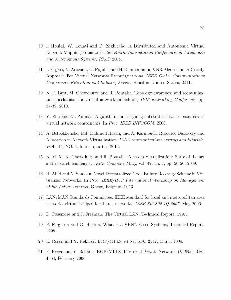
70

[10] I. Houidi, W. Louati and D. Zeghlache. A Distributed and Autonomic Virtual

Network Mapping Framework. the Fourth International Conference on Autonomic

and Autonomous Systems, ICAS, 2008.

[11] I. Fajjari, N. Aitsaadi, G. Pujolle, and H. Zimmermann. VNR Algorithm: A Greedy

Approach For Virtual Networks Reconfigurations. IEEE Globel Communications

Conference, Exhibition and Industry Forum, Houston: United States, 2011.

[12] N. F. Butt, M. Chowdhury, and R. Boutaba. Topology-awareness and reoptimiza-

tion mechanism for virtual network embedding. IFIP networking Conference, pp.

27-39, 2010.

[13] Y. Zhu and M. Ammar. Algorithms for assigning substrate network resources to

virtual network components. In Proc. IEEE INFOCOM, 2006.

[14] A. Belbekkouche, Md. Mahmud Hasan, and A. Karmouch. Resource Discovery and

Allocation in Network Virtualization. IEEE communications surveys and tutorials,

VOL. 14, NO. 4, fourth quarter, 2012.

[15] N. M. M. K. Chowdhury and R. Boutaba. Network virtualization: State of the art

and research challenges. IEEE Commun. Mag., vol. 47, no. 7, pp. 20-26, 2009.

[16] H. Abid and N. Samaan. Novel Decentralized Node Failure Recovery Scheme in Vir-

tualized Networks. In Proc. IEEE/IFIP International Workshop on Management

of the Future Internet, Ghent, Belgium, 2013.

[17] LAN/MAN Standards Committee. IEEE standard for local and metropolitan area

networks virtual bridged local area networks. IEEE Std 802.1Q-2005, May 2006.

[18] D. Passmore and J. Freeman. The Virtual LAN. Technical Report, 1997.

[19] P. Ferguson and G. Huston. What is a VPN?. Cisco Systems, Technical Report,

1998.

[20] E. Rosen and Y. Rekhter. BGP/MPLS VPNs. RFC 2547, March 1999.

[21] E. Rosen and Y. Rekhter. BGP/MPLS IP Virtual Private Networks (VPNs). RFC

4364, February 2006.

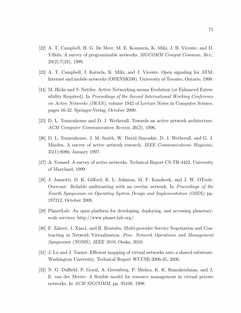
71

[22] A. T. Campbell, H. G. De Meer, M. E. Kounavis, K. Miki, J. B. Vicente, and D.

Villela. A survey of programmable networks. SIGCOMM Comput.Commun. Rev.,

29(2):7(23), 1999.

[23] A. T. Campbell, I. Katzela, K. Miki, and J. Vicente. Open signaling for ATM,

Internet and mobile networks (OPENSIG98). University of Toronto, Ontario, 1998.

[24] M. Hicks and S. Nettles. Active Networking means Evolution (or Enhanced Exten-

sibility Required). In Proceedings of the Second International Working Conference

on Active Networks (IWAN), volume 1942 of Lecture Notes in Computer Science,

pages 16-32. Springer-Verlag, October 2000.

[25] D. L. Tennenhouse and D. J. Wetherall. Towards an active network architecture.

ACM Computer Communication Review, 26(2), 1996.

[26] D. L. Tennenhouse, J. M. Smith, W. David Sincoskie, D. J. Wetherall, and G. J.

Minden. A survey of active network research. IEEE Communications Magazine,

35(1):8086, January 1997.

[27] A. Youssef. A survey of active networks. Technical Report CS-TR-4422, University

of Maryland, 1999.

[28] J. Jannotti, D. K. Gifford, K. L. Johnson, M. F. Kaashoek, and J. W. OToole.

Overcast: Reliable multicasting with an overlay network. In Proceedings of the

Fourth Symposium on Operating System Design and Implementation (OSDI), pp.

197212, October 2000.

[29] PlanetLab: An open platform for developing, deploying, and accessing planetary-

scale services. http://www.planet-lab.org/.

[30] F. Zaheer, J. Xiao1, and R. Boutaba. Multi-provider Service Negotiation and Con-

tracting in Network Virtualization. Proc. Network Operations and Management

Symposium (NOMS), IEEE 2010, Osaka, 2010.

[31] J. Lu and J. Turner. Efficient mapping of virtual networks onto a shared substrate.

Washington University, Technical Report WUCSE-2006-35, 2006.

[32] N. G. Duffield, P. Goyal, A. Greenberg, P. Mishra, K. K. Ramakrishnan, and J.

E. van der Merive. A flexible model for resource management in virtual private

networks. In ACM SIGCOMM, pp. 95108, 1998.

72

[33] C. C. Marquezan, J. C. Nobre, L. Z. Granville, G. Nunzi, D. Dudkowski, and M.

Brunner. Distributed reallocation scheme for virtual network resources. In Proc.

IEEE ICC09, Dresden, Germany, 2009.

[34] I. Houidi, W. Louati, D. Zeghlache, P. Papadimitriou, and L. Mathy. Adaptive

virtual network provisioning. In Proc. ACM SIGCOMM Workshop on Virtualized

Infrastructure Systems and Architectures (VISA10), New Delhi, India, 2010.

[35] I. Houidi, W. Louati, D. Zeghlache, and S. Baucke. Virtual resource description

and clustering for virtual network discovery. In Proc. IEEE ICC09 Workshops,

Dresden, Germany, 2009.

[36] J. He, R. Zhang-Shen, L. Ying, C. Lee, J. Rexford, and M. Chiang. Davinci:

Dynamically adaptive virtual networks for a customized internet. In Proc. ACM

CoNEXT08, Madrid, Spain, 2008.

[37] A. Bavier, M. Bowman, D. Culler, B. Chun, S. Karlin, S. Muir, L. Peterson, T.

Roscoe, T. Spalink, and M. Wawrzoniak. Operating System Support for Planetary-

Scale Network Services. In Proc. Networked Systems Design and Implementation,

Mar. 2004.

[38] Y. Wang , E. Keller, B. Biskeborn , J. van der Merwe and J. Rexford. Virtual

routers on the move : live router migration as a network-management primitive.

SIGCOMM, pp. 231-242. ACM, New York, 2008.

[39] J. F. Botero and X. Hesselbach. The bottlenecked virtual network problem in

bandwidth allocation for network virtualization. In Proc. IEEE Latin-American

Conference on Communications (LATINCOM09), Medeln, Colombia, 2009.

[40] M. Bienkowski, A. Feldmann, D. Jurca, W. Keller, G. Schaffrath, S. Schmid,

and J. Widmer. Competitive analysis for service migration in vnets. In Proc.

ACM SIGCOMM Workshop on Virtualized Infrastructure Systems and Architec-

tures (VISA10), New Delhi, India, 2010.

[41] W.-L. Yeow, C. Westphal, and U. C. Kozat. Designing and embedding reliable

virtual infrastructures. In Proc. ACM SIGCOMM Workshop on Virtualized Infras-

tructure Systems and Architectures (VISA10), New Delhi, India, 2010.

73

[42] B. Porter, F. Taiani and G. Coulson. Generalizing Repair for Overlay Networks.

Computing Department, Lancaster University, UK, Technical Report, PTC-06-01,

October 2006.

[43] I. Stoica, R. Morris, D. Karger, M. F. Kaashoek, and H. Balakrishnan. Chord: A

scalable peer-to-peer lookup service for internet applications. In Proceedings of

the 2001 conference on applications, technologies, architectures, and protocols for

computer communications. ACM Press, pp. 149-160, 2001.

[44] E. Keller, R. Lee, and J. Rexford. Accountability in Hosted Virtual Networks. ACM

978-1-60558-595-6/09/08,VISA09, August 17, 2009.

[45] J. M. Aldous and R. J. Wilson. Graphs and applications: An introductory ap-

proach. Faculty of Mathmematics and Computing, Open University, Walton Hall,

Milton Keynes, UK, 2000.

[46] R. Neapolitan and k. Naimipour. Foundations of Algorithms Using C++ Pseu-

docode. Third Edition, Jones and Bartlett publishers, Sudbury, massachusetts,

1998.

[47] B. Ye Wu and K.-M. Chao. Spanning Trees and Optimazation Problems. Discrete

mathematics and its applications, ChapmanHall/CRC, Kenneth H. Rosen, New

York(USA), 2004.

[48] GENI: Global Environment for Network Innovations. http://www.geni.net/.

[49] ”ViNE-Yard,” http://www.mosharaf.com/ViNE-Yard.tar.gz.

[50] E. Zegura, K. Calvert, and S. Bhattacharjee. How to model an Internetwork. In

Proceedings of IEEE INFOCOM, pp. 594-602, 1996.