notes on tor and ext contents 1. basic homological algebra 1

NOTES ON TOR AND EXT

Contents

1. Basic homological algebra 11.1. Chain complexes 21.2. Maps and homotopies of maps of chain complexes 21.3. Tensor products of chain complexes 31.4. Short and long exact sequences 31.5. Dual cochain complexes and Hom complexes 41.6. Relations between ⊗ and Hom 42. The universal coefficient and Kunneth theorems 52.1. Universal coefficients in homology 52.2. The Kunneth theorem 62.3. Universal coefficients in cohomology 72.4. Proof of the universal coefficient theorem 82.5. Kunneth relations for cochain complexes 93. Torsion products 103.1. Projective resolutions 103.2. The definition and properties of Tor 113.3. Change of rings 133.4. Pairings and products 143.5. A sample computation 154. Ext groups 164.1. Two identities between Hom functors 164.2. Injective resolutions 174.3. The definition and properties of Ext 184.4. Change of rings 194.5. Extensions 204.6. Long extensions and the Yoneda product 204.7. Equivalences of long extensions 214.8. Pairings of Ext groups 23

To make life perhaps a little easier for you, I thought I would bang out somenotes. Be warned, these may be full of misprints. To ease texing, the first twosections are adapted from my book “A Concise Course in Algebraic Topology”.

1. Basic homological algebra

Let R be a commutative ring. The main example will be R = Z. We developsome rudimentary homological algebra in the category of R-modules.

1

2 NOTES ON TOR AND EXT

1.1. Chain complexes. A chain complex over R is a sequence of maps of R-modules

· · · −→ Xi+1di+1

−−−→ Xidi−→ Xi−1 −→ · · ·

such that di ◦di+1 = 0 for all i. We generally abbreviate d = di. A cochain complexover R is an analogous sequence

· · · −→ Y i−1 di−1

−−−→ Y i di

−→ Y i+1 −→ · · ·

with di ◦ di−1 = 0. In practice, we usually require chain complexes to satisfyXi = 0 for i < 0 and cochain complexes to satisfy Y i = 0 for i < 0. Withoutthese restrictions, the notions are equivalent since a chain complex {Xi, di} can berewritten as a cochain complex

{

X−i, d−i}

, and vice versa.An element of the kernel of di is called a cycle and an element of the image of di+1

is called a boundary. We say that two cycles are “homologous” if their differenceis a boundary. We write Bi(X) ⊂ Zi(X) ⊂ Xi for the submodules of boundariesand cycles, respectively, and we define the ith homology group Hi(X) to be thequotient module Zi(X)/Bi(X). We write H∗(X) for the sequence of R-modulesHi(X). We understand “graded R-modules” to be sequences of R-modules such asthis (and we never take the sum of elements in different gradings).

1.2. Maps and homotopies of maps of chain complexes. A map f : X −→ X ′

of chain complexes is a sequence of maps of R-modules fi : Xi −→ X ′i such that

d′i ◦ fi = fi−1 ◦ di for all i. That is, the following diagram commutes for each i:

Xi

fi //

di

��

X ′i

d′

i

��Xi−1

fi−1

// X ′i−1.

It follows that fi(Bi(X)) ⊂ Bi(X′) and fi(Zi(X)) ⊂ Zi(X

′). Therefore f inducesa map of R-modules f∗ = Hi(f) : Hi(X) −→ Hi(X

′).A chain homotopy s : f ≃ g between chain maps f, g : X −→ X ′ is a sequence

of homomorphisms si : Xi −→ X ′i+1 such that

d′i+1 ◦ si + si−1 ◦ di = fi − gi

for all i. Chain homotopy is an equivalence relation since if t : g ≃ h, then s + t ={si + ti} is a chain homotopy f ≃ h.

Lemma 1.1. Chain homotopic maps induce the same homomorphism of homologygroups.

Proof. Let s : f ≃ g, f, g : X −→ X ′. If x ∈ Zi(X), then

fi(x) − gi(x) = d′i+1si(x),

so that fi(x) and gi(x) are homologous. �

NOTES ON TOR AND EXT 3

1.3. Tensor products of chain complexes. The tensor product (over R) ofchain complexes X and Y is specified by letting

(X ⊗ Y )n =∑

i+j=n

Xi ⊗ Yj .

When Xi and Yi are zero for i < 0, the sum is finite, but we don’t need to assumethis. The differential is specified by

d(x ⊗ y) = d(x) ⊗ y + (−1)ix ⊗ d(y)

for x ∈ Xi and y ∈ Yj . The sign ensures that d ◦ d = 0. We may write this as

d = d ⊗ id + id⊗ d.

The sign is dictated by the general rule that whenever two entities to which degreesm and n can be assigned are permuted, the sign (−1)mn should be inserted. In thepresent instance, when calculating (id⊗ d)(x ⊗ y), we must permute the map d ofdegree −1 with the element x of degree i.

We regard R-modules M as chain complexes concentrated in degree zero, andthus with zero differential. For a chain complex X , there results a chain complexX ⊗ M ; H∗(X ⊗ M) is called the homology of X with coefficients in M .

Define a chain complex I by letting I0 be the free Abelian group with twogenerators [0] and [1], letting I1 be the free Abelian group with one generator [I]such that d([I]) = [0]− [1], and letting Ii = 0 for all other i. We could just as welluse free R-modules, but it is nice to have just the single complex I . Observe thatthe tensor product M ⊗ A over Z of an R-module M and an Abelian group A isan R-module via r(m ⊗ a) = (ra) ⊗ a. Similarly, the tensor product over Z of anR-chain complex X and a Z-chain complex Y is an R-chain complex.

Lemma 1.2. A chain homotopy s : f ≃ g between chain maps f, g : X −→ X ′

determines and is determined by a chain map h : X⊗I −→ X ′ such that h(x, [0]) =f(x) and h(x, [1]) = g(x).

Proof. Let s correspond to h via (−1)is(x) = h(x ⊗ [I]) for x ∈ Xi. The relation

d′i+1(si(x)) = fi(x) − gi(x) − si−1(di(x))

corresponds to the relation d′h = hd by the definition of our differential on I . Thesign in the correspondence would disappear if we replaced by X⊗I by I ⊗X . �

1.4. Short and long exact sequences. A sequence M ′ f−→ M

g−→ M ′′ of modules

is exact if im f = ker g. If M ′ = 0, this means that g is a monomorphism; ifM ′′ = 0, it means that f is an epimorphism. A longer sequence is exact if it isexact at each position. A short exact sequence of chain complexes is a sequence

0 −→ X ′ f−→ X

g−→ X ′′ −→ 0

that is exact in each degree. Here 0 denotes the chain complex that is the zeromodule in each degree.

Proposition 1.3. A short exact sequence of chain complexes naturally gives riseto a long exact sequence of R-modules

· · · −→ Hq(X′)

f∗

−→ Hq(X)g∗

−→ Hq(X′′)

∂−→ Hq−1(X

′) −→ · · · .


Proof. Write [x] for the homology class of a cycle x. We define the “connectinghomomorphism” ∂ : Hq(X

′′) −→ Hq−1(X′) by ∂[x′′] = [x′], where f(x′) = d(x) for

some x such that g(x) = x′′. There is such an x since g is an epimorphism, andthere is such an x′ since gd(x) = dg(x) = 0. It is a standard exercise in “diagramchasing” to verify that ∂ is well defined and the sequence is exact. Naturalitymeans that a commutative diagram of short exact sequences of chain complexesgives rise to a commutative diagram of long exact sequences of R-modules. Theessential point is the naturality of the connecting homomorphism, which is easilychecked. �

1.5. Dual cochain complexes and Hom complexes. For a chain complex X =X∗, we define the dual cochain complex X∗ by setting

Xn = Hom(Xn, R) and dn = (−1)n Hom(dn+1, id).

As with tensor products, we understand Hom to mean HomR when R is clear fromthe context. On elements, for an R-map f : Xn −→ R and an element x ∈ Xn+1,

(dnf)(x) = (−1)nf(dn(x)).

More generally, for an R-module M , we define a cochain complex Hom(X, M) inthe same way. The sign is conventional. In analogy with the notation H∗(X ; M) =H∗(X ⊗ M), we write

H∗(X ; M) = H∗(Hom(X, M)).

More generally, for a cochain complex Y , define

Hom(X, Y )n = ×q Hom(Xq, Yn−q)

with differential δ specified by

(δf)(x) = d(f(x)) − (−1)nf(d(x))

More explicitly, writing f = (fq), fq : Xq −→ Y n−q, this means that δ(f) = (gq),where gq : Xq −→ Y n+1−q is given on x ∈ Xq as the difference of dn−q(fq(x)) and(−1)nfq−1dq(x). When Y = M is concentrated in degree 0, this agrees with theprevious definition.

Note that if we take X to be just a chain complex of Z-modules and take Hom’sover Z, then the definition still makes sense and gives a complex of R-modules.We have defined Hom’s between chain and cochain complexes in the way that theyare most frequently used, but, when thinking categorically it makes more sense toregrade all cochain complexes as chain complexes and redefine

Hom(X, Y )n = ×q Hom(Xq, Yq+n).

1.6. Relations between ⊗ and Hom. We record a few observations relating ⊗and Hom of complexes, starting with relations between ⊗ and Hom on the categoryof R-modules. For R-modules L, M , and N , we have an adjunction

Hom(L ⊗ M, N) ∼= Hom(L, Hom(M, N)).

We also have a natural homomorphism

Hom(L, M) ⊗ N −→ Hom(L, M ⊗ N),

and this is an isomorphism if either L or N is a finitely generated projective R-module. Again, we have a natural map

Hom(L, M) ⊗ Hom(L′, M ′) −→ Hom(L ⊗ L′, M ⊗ M ′),


which is an isomorphism if L and L′ are finitely generated and projective or if L isfinitely generated and projective and M = R.

We can replace L and L′ by chain complexes and obtain similar maps, insertingsigns where needed. For example, a chain homotopy X ⊗I −→ X ′ between chainmaps f, g : X −→ X ′ induces a chain map

Hom(X ′, M) −→ Hom(X ⊗ I , M) ∼= Hom(I , Hom(X, M)) ∼= Hom(X, M) ⊗ I∗,

where I ∗ = Hom(I , R). It should be clear that this implies that our originalchain homotopy induces a homotopy of cochain maps

f∗ ≃ g∗ : Hom(X ′, M) −→ Hom(X, M).

2. The universal coefficient and Kunneth theorems

We describe some classical results in homological algebra that explain how tocalculate H∗(X ; M) from H∗(X) ≡ H∗(X ; R) and how to calculate H∗(X ⊗ Y )from H∗(X) ⊗ H∗(Y ). We then describe how to calculate H∗(X ; M) from H∗(X).We again work over a general commutative ring R, and ⊗ and Hom are implicitlyunderstood to be taken over R.

2.1. Universal coefficients in homology. Let X and Y be chain complexesover R. We think of H∗(X) ⊗ H∗(Y ) as a graded R-module which, in degree n, is∑

p+q=n Hp(X) ⊗ Hq(Y ). We define

α : H∗(X) ⊗ H∗(Y ) −→ H∗(X ⊗ Y )

by α([x] ⊗ [y]) = [x ⊗ y] for cycles x and y that represent homology classes [x] and[y]. As a special case, for an R-module M we have

α : H∗(X) ⊗ M −→ H∗(X ⊗ M).

We omit the proof of the following standard result, but we shall shortly give thequite similar proof of a cohomological analogue. Recall that an R-module M is saidto be flat if the functor M ⊗ N is exact (that is, preserves exact sequences in thevariable N). We say that a graded R-module is flat if each of its terms is flat.

We shall treat torsion products, which measure the failure of tensor products tobe exact functors, shortly. For a principal ideal domain (PID) R, the only torsion

product is the first one, denoted TorR1 (M, N). It can be computed by constructing

a short exact sequence

0 −→ F1 −→ F0 −→ M −→ 0

and tensoring with N to obtain an exact seqence

0 −→ TorR1 (M, N) −→ F1 ⊗ N −→ F0 ⊗ N −→ M ⊗ N −→ 0,

where F1 and F0 are free R-modules. That is, we choose an epimorphism F0 −→ Mand note that, since R is a PID, its kernel F1 is also free.

Theorem 2.1 (Universal coefficient). Let R be a PID and let X be a flat chaincomplex over R. Then, for each n, there is a natural short exact sequence

0 −→ Hn(X) ⊗ Mα−→ Hn(X ⊗ M)

β−→ TorR

1 (Hn−1(X), M) −→ 0.

The sequence splits, so that

Hn(X ⊗ M) ∼= (Hn(X) ⊗ M) ⊕ TorR1 (Hn−1(X), M),

but the splitting is not natural.


Remark 2.2. The result holds more generally when R is any ring and the chainsand cycles of X are also flat R-modules.

Corollary 2.3. If R is a field, then

α : H∗(X) ⊗ M −→ H∗(X ; M)

is a natural isomorphism.

2.2. The Kunneth theorem. The universal coefficient theorem in homology is aspecial case of the Kunneth theorem.

Theorem 2.4 (Kunneth). Let R be a PID and let X be a flat chain complex andY be any chain complex. Then, for each n, there is a natural short exact sequence

0 −→∑

p+q=n

Hp(X)⊗Hq(Y )α−→ Hn(X⊗Y )

β−→

∑

p+q=n−1

TorR1 (Hp(X), Hq(Y )) −→ 0.


Hn(X ⊗ Y ) ∼= (∑

p+q=n

Hp(X) ⊗ Hq(Y )) ⊕ (∑

p+q=n−1

TorR1 (Hp(X), Hq(Y ))),


This applies directly to the computation of the homology of the Cartesian prod-uct of CW complexes X and Y in view of the isomorphism

C∗(X × Y ) ∼= C∗(X) ⊗ C∗(Y ).


α : H∗(X) ⊗ H∗(Y ) −→ H∗(X ⊗ Y )


We prove the corollary to give the idea. The general case is proved by an elab-oration of the argument. There is a simple but important technical point to makehere. Let us for the moment remember to indicate the ring over which we are takingtensor products. For chain complexes X and Y over Z, we have

(X ⊗Z R) ⊗R (Y ⊗Z R) ∼= (X ⊗Z Y ) ⊗Z R.

We can therefore use the corollary to compute H∗(X ⊗Z Y ; R) from H∗(X ; R) andH∗(Y ; R).

Proof of the corollary. Assume first that Xi = 0 for i 6= p, so that X = Xp is justan R-module with no differential. The square commutes and the row and column


are exact in the diagram

0

��0 // Bq(Y ) // Zq(Y )

��

// Hq(Y ) // 0.

Yq+1dq+1

//

dq+1

OO

Yq

dq

��Yq−1

Since all modules over a field are free and thus flat, this remains true when wetensor the diagram with Xp. This proves that if n = p + q, then

Zn(Xp ⊗ Y ) = Xp ⊗ Zq(Y ), Bn(Xp ⊗ Y ) = Xp ⊗ Bq(Y ),

and therefore

Hn(X ⊗ Y ) = Xp ⊗ Hq(Y ).

In the general case, regard the graded modules Z(X) and B(X) as chain complexeswith zero differential. The exact sequences

0 −→ Zp(X) −→ Xp

dp

−→ Bp−1(X) −→ 0

of R-modules define a short exact seqence of chain complexes since dp−1 ◦ dp = 0.Define the suspension of a graded R-module N by (ΣN)n+1 = Nn. Tensoring withY , we obtain a short exact sequence of chain complexes

0 −→ Z(X) ⊗ Y −→ X ⊗ Y −→ ΣB(X) ⊗ Y −→ 0.

It follows from the first part and additivity that

H∗(Z(X) ⊗ Y ) = Z(X) ⊗ H∗(Y ) and H∗(ΣB(X) ⊗ Y ) = ΣB(X) ⊗ H∗(Y ).

Moreover, by inspection of definitions, the connecting homomorphism of the longexact sequence of homology modules associated to our short exact sequence of chaincomplexes is just the inclusion B ⊗ H∗(Y ) −→ Z ⊗ H∗(Y ). In particular, the longexact sequence breaks up into short exact sequences

0 −→ B(X) ⊗ H∗(Y ) −→ Z(X) ⊗ H∗(Y ) −→ H∗(X ⊗ Y ) −→ 0.

However, since tensoring with H∗(Y ) is an exact functor, the cokernel of the inclu-sion B ⊗ H∗(Y ) −→ Z ⊗ H∗(Y ) is H∗(X) ⊗ H∗(Y ). The conclusion follows. �

2.3. Universal coefficients in cohomology. We have a cohomological version ofthe universal coefficient theorem. We shall treat Ext modules, which measure thefailure of Hom to be an exact functor, shortly. For a PID R, the only Ext moduleis the first one, denoted Ext1R(M, N). It can be computed by constructing a shortexact sequence

0 −→ F1 −→ F0 −→ M −→ 0

and applying Hom to obtain an exact seqence

0 −→ Hom(M, N) −→ Hom(F0, N) −→ Hom(F1, N) −→ Ext1R(M, N) −→ 0,

where F1 and F0 are free R-modules.


For each n, define

α : Hn(Hom(X, M)) −→ Hom(Hn(X), M)

by letting α[f ]([x]) = f(x) for a cohomology class [f ] represented by a “cocycle”f : Xn −→ M and a homology class [x] represented by a cycle x. It is easy tocheck that f(x) is independent of the choices of f and x since x is a cycle and f isa cocycle.

Theorem 2.6 (Universal coefficient). Let R be a PID and let X be a free chaincomplex over R. Then, for each n, there is a natural short exact sequence

0 −→ Ext1R(Hn−1(X), M)β−→ Hn(X ; M)

α−→ Hom(Hn(X), M) −→ 0.


Hn(X ; M) ∼= Hom(Hn(X), M) ⊕ Ext1R(Hn−1(X), M),



α : H∗(X ; M) −→ Hom(H∗(X), M)


Again, there is a technical point to be made here. If X is a complex of freeAbelian groups and M is an R-module, such as R itself, then

HomZ(X, M) ∼= HomR(X ⊗Z R, M).

One way to see this is to observe that, if B is a basis for a free Abelian group F , thenHomZ(F, M) and HomR(F ⊗Z R, M) are both in canonical bijective correspondencewith maps of sets B −→ M . More algebraically, a homomorphism f : F −→ M ofAbelian groups determines the corresponding map of R-modules as the compositeof f ⊗ id and the action of R on M :

F ⊗Z R −→ M ⊗Z R −→ M.

2.4. Proof of the universal coefficient theorem. We need two properties ofExt in the proof. First, Ext1R(F, M) = 0 for a free R-module F . Second, when Ris a PID, a short exact sequence

0 −→ L′ −→ L −→ L′′ −→ 0

of R-modules gives rise to a six-term exact sequence

0 −→ Hom(L′′, M) −→ Hom(L, M) −→ Hom(L′, M)δ−→ Ext1R(L′′, M) −→ Ext1R(L, M) −→ Ext1R(L′, M) −→ 0.

Proof of the universal coefficient theorem. We write Bn = Bn(X), Zn = Zn(X),and Hn = Hn(X) to abbreviate notation. Since each Xn is a free R-module and Ris a PID, each Bn and Zn is also free. We have short exact sequences

0 // Bnin // Zn

πn // Hn// 0

and

0 // Zn

jn // Xn

dn // Bn−1σn

oo_ _ _// 0;


we choose a splitting σn of the second. Writing f∗ = Hom(f, M) consistently, weobtain a commutative diagram with exact rows and columns

0 0

��0 // Hom(Hn, M)

π∗

n // Hom(Zn, M)i∗n //

OO

Hom(Bn, M)

d∗

n+1

��· · · // Hom(Xn−1, M)

d∗

n //

j∗n−1

��

Hom(Xn, M)

j∗n

OO

d∗

n+1 //

σ∗

n

��

�

Hom(Xn+1, M) // · · ·

Hom(Zn−1, M)i∗n−1

//

��

Hom(Bn−1, M)δ

//

d∗

n

OO

0

66ll

ll

ll

l

Ext1R(Hn−1, M) // 0

0 0

OO

By inspection of the diagram, we see that the canonical map α coincides with thecomposite

Hn(X ; M) = ker d∗n+1/ im d∗n = ker i∗nj∗n/ im d∗ni∗n−1

j∗n−→ im π∗

n

(π∗

n)−1

−−−−→ Hom(Hn, M).

Since j∗n is an epimorphism, so is α. The kernel of α is im d∗n/ im d∗ni∗n−1, and

δ(d∗n)−1 maps this group isomorphically onto Ext1R(Hn−1, M). The composite δσ∗n

induces the required splitting. �

2.5. Kunneth relations for cochain complexes. If Y and Y ′ are cochain com-plexes, then we have the natural homomorphism

α : H∗(Y ) ⊗ H∗(Y ′) −→ H∗(Y ⊗ Y ′)

given by α([y]⊗[y′]) = [y⊗y′], exactly as for chain complexes. In fact, by regrading,we may view this as a special case of the map for chain complexes. The Kunneththeorem applies to this map. For its flatness hypothesis, it is useful to rememberthat, for any Noetherian ring R, the dual Hom(F, R) of a free R-module is a flatR-module.

As indicated in §1.6, if Y = Hom(X, M) and Y ′ = Hom(X ′, M ′) for chaincomplexes X and X ′ and R-modules M and M ′, then we also have the map ofcochain complexes

ω : Hom(X, M) ⊗ Hom(X ′, M ′) −→ Hom(X ⊗ X ′, M ⊗ M ′)

specified by the formula

ω(f ⊗ f ′)(x ⊗ x′) = (−1)(deg f ′)(deg x)f(x) ⊗ f ′(x′).

Also writing ω for the map it induces on cohomology, we then have the composite

ω ◦ α : H∗(X ; M)⊗ H∗(X ′; M ′) −→ H∗(X ⊗ X ′; M ⊗ M ′).

When M = M ′ = A is a commutative R-algebra, we may compose with the map

H∗(X ⊗ X ′; A ⊗ A) −→ H∗(X ⊗ X ′; A)

induced by the multiplication of A to obtain a map

H∗(X ; A) ⊗ H∗(X ′; A) −→ H∗(X ⊗ X ′; A).


The cases most commonly used are when R = Z and A is either Z or a field. Forexample, this is a starting point for the definition of the cup product in topology.

3. Torsion products

We give a quick development of the basic theory of torsion products. Here wechange our point of view and work more generally with non-commutative rings Rand their right and left modules. Thus, in general, M ⊗R N is only an Abeliangroup. When R is commutative, all of our functors take values in the category ofR-modules rather than just Abelian groups.

3.1. Projective resolutions. We work with right R-modules here, but we couldequally well work with left R-modules. Recall that an R-module P is said to beprojective if for each epimorphism g : M −→ N and each map f : P −→ N , thereexists a map f : P −→ M such that g ◦ f = f . This means that

Hom(id, g) : HomR(P, M) −→ Hom(P, N)

is an epimorphism. There is a standard characterization.

Lemma 3.1. A module P is projective if and only if it is a direct summand of afree module. Any projective module is flat.

Proof. It is clear that R itself is projective and any direct sum of projective modulesis projective. Therefore every free module is projective. If there is a module Q suchthat P ⊕Q = F is free, then, using the inclusion P −→ F and projection F −→ P ,we see that P is projective. If P is projective and g : F −→ P is an epimorphismwith F free, as can always be chosen, then application of projectivity to the identitymap P −→ P shows that P is a direct summand of F . Since direct sums and directsummands of flat modules are flat, the second statement follows. �

Let M be an R-module. A complex of R-modules over M is a complex of theform

· · · −→ Xi+1di+1

−−−→ Xidi−→ Xi−1 −→ · · · −→ X0

ε−→ M −→ 0.

It is a projective (or free or flat) complex over M if each Xi is projective (or freeor flat). It is a resolution of M if the displayed sequence is exact. It is appropriateto think of M itself as a complex concentrated in degree 0 and ε : X −→ M as amorphism of complexes. If X is a resolution of M , then ε induces an isomorphismon homology since Coker d1 = M .

Lemma 3.2. Every R-module M has a projective resolution.

Proof. Every module is a quotient of a free module. Start with an epimorphismε : X0 −→ M with X0 free. Then choose an epimorphism X1 −→ Ker ε, with X1

free and let d1 be its composite with the inclusion Ker ε ⊂ X0. Continue inductivelyto construct epimorphisms Xi+1 −→ Ker di. �

Projective resolutions are unique up to chain homotopy equivalence, as we seeby taking f = id in the following result.

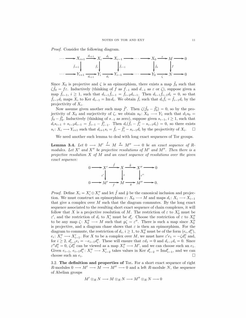
Lemma 3.3. Let f : M −→ N be a map of R-modules. Let ε : X −→ M be aprojective complex over M and let ζ : Y −→ N be a resolution of N . Then there isa map f : X −→ Y of chain complexes such that ζ ◦ f = f ◦ ε, and f is unique upto chain homotopy.


Proof. Consider the following diagram.

· · · // Xi+1di+1 //

fi+1

��

Xidi //

fi

��

Xi−1//

fi−1

��

· · · // X0

f0

��

ε // M //

f

��

0

· · · // Yi+1di+1

// Yidi

// Yi−1// · · · // Y0

ζ// N // 0

Since X0 is projective and ζ is an epimorphism, there exists a map f0 such thatζf0 = fε. Inductively (thinking of f as f−1 and d−1 as ε or ζ), suppose given a

map fi−1, i ≥ 1, such that di−1fi−1 = fi−2di−1. Then di−1fi−1di = 0, so that

fi−1di maps Xi to Ker di−1 = Im di. We obtain fi such that difi = fi−1di by theprojectivity of Xi.

Now assume given another such map f ′. Then ζ(f0 − f ′0) = 0, so by the pro-

jectivity of X0 and surjectivity of ζ, we obtain s0 : X0 −→ Y1 such that d1s0 =f0 − f ′

0. Inductively (thinking of s−1 as zero), suppose given si−1, i ≥ 1, such that

disi−1 + si−2di−1 = fi−1 − f ′i−1. Then di(fi − f ′

i − si−1di) = 0, so there exists

si : Xi −→ Yi+1 such that di+1si = fi − f ′i − si−1di by the projectivity of Xi. �

We need another such lemma to deal with long exact sequences of Tor groups.

Lemma 3.4. Let 0 −→ M ′ f−→ M

g−→ M ′′ −→ 0 be an exact sequence of R-

modules. Let X ′ and X ′′ be projective resolutions of M ′ and M ′′. Then there is aprojective resolution X of M and an exact sequence of resolutions over the givenexact sequence:

0 // X ′f //

ε′

��

Xg //

ε

��

X ′′ //

ε′′

��

0

0 // M ′

f// M g

// M ′′ // 0.

Proof. Define Xi = X ′i ⊕X ′′

i and let f and g be the canonical inclusion and projec-tion. We must construct an epimorphism ε : X0 −→ M and maps di : Xi −→ Xi−1

that give a complex over M such that the diagram commutes. By the long exactsequence associated to the resulting short exact sequence of chain complexes, it willfollow that X is a projective resolution of M . The restriction of ε to X ′

0 must beε′, and the restriction of di to X ′

i must be d′i. Choose the restriction of ε to X ′′0

to be any map ζ : X ′′0 −→ M such that gζ = ε′′. There is such a map since X ′′

0

is projective, and a diagram chase shows that ε is then an epimorphism. For thediagram to commute, the restriction of di, i ≥ 1, to X ′′

0 must be of the form (ei, d′′i ),

ei : X ′′i −→ X ′

i−1. For X to be a complex over M , we must have ε′e1 = −ζd′′1 and,for i ≥ 2, d′i−1ei = −ei−1d

′′i . These will ensure that εd1 = 0 and di−1di = 0. Since

ε′′d′′1 = 0, ζd′′1 can be viewed as a map X ′′1 −→ M ′, and we can choose such an e1.

Given ei−1, ei−1d′′i : X ′′

i −→ X ′i−2 takes values in Ker d′i−2 = Imd′i−1, and we can

choose such an ei. �

3.2. The definition and properties of Tor. For a short exact sequence of rightR-modules 0 −→ M ′ −→ M −→ M ′′ −→ 0 and a left R-module N , the sequenceof Abelian groups

M ′ ⊗R N −→ M ⊗R N −→ M ′′ ⊗R N −→ 0


is exact, but the left-most arrow need not be a monomorphism. We say that ⊗R

is right exact. Torsion products measure the deviation from exactness. Here is anomnibus theorem that states the basic properties of torsion products.

Theorem 3.5. There are Abelian group–valued functors TorRn (M, N) of right R-

modules M and left R-modules N , together with natural connecting homomorphisms

∂ : TorRn (M ′′, N) −→ TorR

n−1(M′, N) and ∂ : TorR

n (M, N ′′) −→ TorRn−1(M, N ′)

for short exact sequences

0 −→ M ′ −→ M −→ M ′′ −→ 0 and 0 −→ N ′ −→ N −→ N ′′ −→ 0.

These satisfy the following properties.

(i) TorRn (M, N) = 0 for n < 0.

(ii) TorR0 (M, N) is naturally isomorphic to M ⊗R N .

(iii) TorRn (M, N) = 0 for n > 0 if either M or N is projective.

(iv) The following sequences are exact.

· · · −→ TorRn (M ′, N) −→ TorR

n (M, N) −→ TorRn (M ′′, N) −→ TorR

n−1(M′, N) −→ · · ·

· · · −→ TorRn (M, N ′) −→ TorR

n (M, N) −→ TorRn (M, N ′′) −→ TorR

n−1(M, N ′) −→ · · ·

For each fixed N , the functors TorRn (M, N) of M together with the natural con-

necting homomorphisms ∂ : TorRn (M ′′, N) −→ TorR

n−1(M′, N) on exact sequences

0 −→ M ′ f−→ M

g−→ M ′′ −→ 0 are uniquely determined up to isomorphism by

(i)—(iv), and similarly for each fixed M .

Proof. The naturality statements imply that the long exact sequences of (iv) arefunctorial on short exact sequences. For the existence statement, let us fix N .Choose a projective resolution X of M . Define

TorR∗ (M, N) = H∗(X ⊗R N)

Since chain homotopic maps of complexes induce the same map on homology,Lemma 3.3 shows that this is well-defined up to natural isomorphism and givesa functor of M . Manifestly, it also gives a functor of N . Since ⊗R is right exact,(ii) is clear. Since the identity map X0 = M −→ M is a projective resolution of aprojective module M and since projective modules are flat, both parts of (iii) arealso clear. We define the first map ∂ and derive the first long exact sequence of(iv) by use of Lemma 3.4. We define the second map ∂ and derive the second longexact sequence by use of the short exact sequence of chain complexes

0 −→ X ⊗ N ′ −→ X ⊗ N −→ X ⊗ N ′′ −→ 0.

Here exactness holds by the projectivity and thus flatness of the Xi.For the axiomatization, we proceed by induction on n, starting from (i) and (ii).

If we have two systems of functors and natural connecting homomorphisms andwe have proven they are isomorphic through stage (n − 1), then a diagram chasestarting from short exact sequences 0 −→ M ′ −→ M −→ M ′′ −→ 0 where M isfree shows that they are isomorphic at the stage n.

We can reverse the roles of M and N in our original construction, starting froma projective resolution of N . We again have all of the properties (i) – (iv), so bythe uniqueness we obtain the same sequence of functors and natural connectinghomomorphisms. Moreover, we can also check that H∗(X ⊗R Y ) gives functorsand natural connecting homomorphisms that satisfy the axioms. Altenatively, we


can observe that the morphisms of complexes X −→ M and Y −→ N inducemorphisms of complexes

X ⊗R M X ⊗R Y //oo Y ⊗R N.

Either by a direct, hands on, Kunneth type argument, or more elegantly by anapplication of the theory of spectral sequences if one knows about that, one cancheck directly that these give isomorphisms. �

3.3. Change of rings. In applications, it is very often the case that we use furtherstructure on torsion products. We describe some of this here and in the next section.We take the opportunity to introduce and use some standard and important adjointfunctors on the way.

In this section, we fix a homomorphism of rings f : R −→ S. Let M and P bea right R module and a right S-module, and let g : M −→ P be an f -equivariantmap, meaning that g(mr) = g(m)f(r). Similarly, let N and Q be a left R-moduleand a left S-module and let h : N −→ Q be f -equivariant, h(rn) = f(r)h(n). Weshall obtain a map

(3.6) Torf∗(g, h) : TorR

∗ (M, N) −→ TorS∗ (P, Q).

This allows us to view Tor as a functor of all three variables.Let us write f∗ for the pullback of action functor MS −→ MR, where MR

denotes the category of right R-modules. Thus f∗P is P with the right R-actionpr = pf(r). Clearly g is just a map of right R-modules M −→ f∗P . The functorf∗ has left and right adjoints, often denoted f! and f∗, that are given by extensionand coextension of scalars. Explicitly,

f!M = M ⊗R S and f∗M = HomR(S, M).

We are using that S is both a left and a right S-module and therefore a left andright R-module via f . In defining M ⊗R S, we use the left action of R to define thetensor product and use the right action of S to give M ⊗R S an S-action, whereasHomR(S, M) is the Abelian group of maps of right R-modules k : S −→ M , withright S-action given by (ks)(s′) = k(ss′). That is, it is induced by the left actionof S on itself. The adjunctions read

HomS(f!M, P ) ∼= HomR(M, f∗P ) and HomR(f∗P, M) ∼= HomS(P, f∗M).

The easy verifications are left to the reader.The functor f! takes R to S and preserves direct sums, hence it takes R-projective

modules to S-projective modules. If f∗S is flat as an R-module, in which case wesay that f is a “flat extension” of R, then f! takes exact sequences of R-modulesto exact sequences of S-modules. Now Lemma 3.3 gives the following result.

Lemma 3.7. Let X be a projective R-resolution of M and Y be a projective S-resolution of P . Then there is a map g : f!X −→ Y of S-projective complexes overthe adjoint g : f!M −→ P of the map g : M −→ f∗P . It is a map of projectiveresolutions if S is a flat extension of R.

We agree to write f! for both of the functors M ⊗R S and S ⊗R N . We have thenatural homomorphism of Abelian groups

ζ : M ⊗R N −→ f!M ⊗S f!N ∼= M ⊗R S ⊗R N


specified by ζ(m⊗n) = m⊗ 1⊗n. With the notations of the previous lemma, and

using the adjoint h : f!N −→ Q of h : N −→ f∗Q, this gives a natural composite

X ⊗R N −→ f!X ⊗S f!N −→ Y ⊗S Q.

Passing to homology, we obtain the promised map (3.6). A moment’s reflectionshows that it factors naturally as the composite

TorR∗ (M, N)

Torid∗

(η,η)// TorR∗ (f∗f!M, f∗f!N)

Torf∗(id,id)// TorS

∗ (f!M, f!N)Torf

∗(g,h)// TorS

∗ (P, Q)

where η : M −→ f∗f!M is the unit of the adjunction, η(m) = m ⊗ 1 ∈ M ⊗R S.

Remember that when R is commutative, TorR∗ (M, N) is a graded R-module.

The following result could be obtained a little more directly but it illustrates ideasto derive it from what we have done.

Proposition 3.8. Let T be a multiplicative subset of a commutative ring R andlet S = RT = R[T−1] be the localization of R at T . For all R-modules M and N ,the canonical map

TorR∗ (M, N) −→ TorS

∗ (M ⊗R S, N ⊗R S)

is localization at T .

Proof. The localization functor sends M to f!M = M ⊗R S, where f : R −→ S isthe localization map. Of course, f is a flat extension. The target of our map is anS-module and is therefore T -local. After tensoring with S, our map becomes theisomorphism on homology induced by the canonical isomorphism of chain complexes

(X ⊗R N) ⊗R S ∼= (X ⊗R S) ⊗S (N ⊗R S)

where X is an R-projective resolution of M . �

3.4. Pairings and products. Again let R and S be rings. In applications, it isoften the case that our rings are algebras over a commutative ring k. Taking tensorproducts over k rather than Z and writing ⊗ = ⊗k, the constructions of this sectiongeneralize directly. Let M and N be right and left R-modules, and let P and Q beright and left S-modules. Letting γ be the symmetry isomorphism, R⊗ S is a ringwith product

R ⊗ S ⊗ R ⊗ Sid⊗γ⊗id //R ⊗ R ⊗ S ⊗ S //R ⊗ S

induced by the products of R and S. Similarly, M ⊗ P is a right (R ⊗ S)-modulewith action

M ⊗ P ⊗ R ⊗ Sid×γ×id //M ⊗ R ⊗ P ⊗ S //M ⊗ P

induced by the actions of R on M and S on P , and N ⊗Q is a left R⊗ S-module.Let X be an R-projective resolution of M and Y be a S-projective resolution of

P . Then X ⊗ Y is an R ⊗ S-projective complex over M ⊗ P . Rather than use aKunneth argument to check that it is a resolution, we can map it to a projectiveR⊗S-projective resolution of M ⊗P by use of Lemma 3.3. Using the natural mapα from the tensor product of homologies to the homology of a tensor product, themap

(X ⊗R N) ⊗ (Y ⊗S Q) −→ (X ⊗ Y ) ⊗R⊗S (N ⊗ Q)

induced by id⊗γ ⊗ id gives rise to a natural pairing

(3.9) TorR∗ (M, N) ⊗ TorS(P, Q) −→ TorR⊗S

∗ (M ⊗ P, N ⊗ Q).


Now recall that a ring R is commutative if and only if its product is a map ofrings. In formulas, this means that rr′ss′ = ss′rr′ for all r, r′, s, s′ if and only ifrs = sr for all r and s. Taking r′ = 1 = s′ gives one implication, and the otheris obvious. When we deal with graded rings with products Rm ⊗ Rn −→ Rm+n,we understand commutativity to mean graded commutativity, rs = (−1)mnsr.Formally, that means that we are defining the graded symmetry isomorphism γwith our usual sign convention on interchange.

We say that a ring R is augmented over a ring k if there is an epimorphism ofrings ε : R −→ k. It is especially interesting to consider the quotient homomorphismε : R −→ R/m = k of a local ring R with maximal ideal m.

Theorem 3.10. If R is a commutative ring with augmentation ε : R −→ k, thenTorR

∗ (k, k) is a graded commutative k-algebra.

Proof. We are regarding k as the R-module ε∗k. Writing φ for the products on Rand on k, the required product on TorR

∗ (k, k) is the composite

TorR∗ (k, k) ⊗k TorR

∗ (k, k) −→ TorR⊗R∗ (k ⊗ k, k ⊗ k) −→ TorR

∗ (k, k).

While R is not a k-algebra, the construction just given works with M = N = P = Qto give the first map, and the second map is Torφ(φ, φ) of (3.6). Note that φ induces

an isomorphism k ⊗R k −→ k, so that TorR0 (k, k) ∼= k. It is a straightforward

exercise, left to the reader, that the product on TorR∗ (k, k) is associative, unital,

and graded commutative. �

3.5. A sample computation. It is all very well to define a product, but howdo we compute it? A DGA (differential graded k-algebra) is a k-chain complexA with an associative and unital product A ⊗k A −→ A which is a map of chaincomplexes, meaning d(ab) = d(a)b + (−1)degaad(b). It is (graded) commutative ifab = (−1)degadegbba for all a and b. We can also define the weaker notion of aDGA up to chain homotopy. This is defined in the same way, except that we onlyrequire associativity and unitality up to chain homotopy. The homotopies ensurethat H∗(A) is a graded algebra. For example, the (normalized) singular cochainsof a space with coefficients in k form a cohomologically graded DGA, but it isonly commutative up to chain homotopy, and that is enough to ensure that thecohomology of a space is a commutative k-algebra.

Now return to a commutative ring R with augmentation ε : R −→ k, for examplean augmented k-algebra. Let X be an R-projective resolution of k. Then Lemma 3.3gives that there is a map of (R ⊗ R)-chain complexes φ : X ⊗ X −→ X over theproduct φ : k ⊗ k −→ k, where X is regarded as an (R ⊗ R)-chain complex viathe product R ⊗ R −→ R. Since the product on k is associative, unital, andcommutative, the same result applies to show that the product φ is associative,unital, and (graded) commutative up to chain homotopy. Then X ⊗R k is a DG

k-algebra, and its homology is TorR∗ (k, k) as a k-algebra. This is all that one can

expect in general, but for especially nice rings R, one can find an X which is actuallya DGA, with no need for chain homotopies.

To illustrate, let R be the polynomial algebra k[x] with augmentation determinedby ε(x) = 0. Let X be the graded k-algebra and free right R-module E[y] ⊗k R,where E[y] is the exterior algebra on one generator y of degree 1. Thus y2 = 0, andE[y] is the free k-module with one basis element 1 of degree 0 and one basis elementy of degree 1. Define ε : X −→ k by letting ε(1⊗1) = 1 and ε(y⊗1) = 0 = ε(1⊗x).


Define a differential on X by letting d(y⊗1) = 1⊗x and requiring d to be a map ofR-modules. Then d(y⊗xn) = 1⊗xn+1. Since X has the k-basis {1×xn}∪{y⊗xn}we see that X is an R-free resolution of k. Moreover, it is a differential graded R-algebra, and X ⊗R k is the k-algebra E[y] with zero differential. This proves thecase n = 1 of the following result.

Theorem 3.11. Let R be the polynomial algebra k[x1, · · · , xn]. Then TorR∗ (k, k)

is the exterior algebra E[y1, · · · , yn], where deg(yi) = 1.

Proof. X = E[y1, · · · , yn] ⊗ R is a DG R-algebra with differential determined byd(yi) = xi on generators over R, and it is isomorphic to the tensor product of DGk-algebras

(E[y1] ⊗ k[y1]) ⊗k · · · ⊗k (E[yn] ⊗ k[yn]).

With the evident map to k, it follows that the DGA X is an R-free resolution of k.The differential on X ⊗R k = E[y1, · · · , yn] is zero, and the conclusion follows. �

Since the associated graded k-algebra of a regular local ring R with respect tothe filtration given by the powers of its maximal ideal is a polynomial algebraon n generators, where n is the Krull dimension of R is n, this suggests thatthe conclusion applies equally well to TorR

∗ (k, k). In particular, this suggests that

TorRq (k, k) = 0 for q > n. In fact, we shall see later that much more is true. We

state the result now and prove it later.

Theorem 3.12 (Serre). Let R be a (Noetherian) local ring of Krull dimension

n. If TorRq (k, k) is zero for any q > n, then R is regular. If R is regular, then

TorRq (M, N) = 0 for all R-modules M and N and all q > n and, as a k-algebra,

TorR∗ (k, k) ∼= E[y1, · · · , yn].

4. Ext groups

We give a quick parallel development of the basic theory of ext groups. We againwork with non-commutative rings R and their right and left modules. By default,modules mean left modules, and then HomR(M, N) is the Abelian group of mapsof left R-modules M −→ N . Again, when R is commutative, everything we doworks just as well in the category of R-modules.

4.1. Two identities between Hom functors. For rings R and S, an (R, S)-bimodule M is a left R-module and right S-module with commuting actions, mean-ing that (rm)s = r(ms). When R is commutative, any R-module may be consideredas an (R, R)-bimodule with rm = mr. We record two standard identities. Theirproofs are elementary, but it is fun to use the Yoneda lemma and analogous iden-tities between tensor products to derive them.

Lemma 4.1. Let M be a left R-module, N be a right S-module, and P be an(R, S)-bimodule. Then there is a natural isomorphism of Abelian groups

HomR(M, HomS(N, P )) ∼= HomS(N, HomR(M, P )).

Here the R and S actions on P induce the R and S actions on HomS(N, P ) andHomR(M, P ).


Lemma 4.2. Let M be a right R-module, N be an (R, S)-bimodule, and P be aleft S-module. Then there is a natural isomorphism of Abelian groups

HomS(M ⊗R N, P ) ∼= HomR(M, HomS(N, P )).

Here the S and R actions on N induce the S and R actions on M ⊗R N andHomS(N, P ). The analogous result with left and right reversed also holds.

We shall have immediate use of the following special case of the reversed version.Here we specialize S to Z. We take N = R, regarded as a right R-module, notingthat any right R-module can be viewed as a (Z, R)-bimodule.

Lemma 4.3. Let M be a left R-module and P be an Abelian group. Then there isa natural isomorphism of Abelian groups

HomZ(M, P ) ∼= HomR(M, HomZ(R, P )).

4.2. Injective resolutions. Recall that modules mean left modules. A moduleI is said to be injective if for each monomorphism e : L −→ M and each mapf : L −→ I, there exists a map f : M −→ I such that f ◦ e = f . This means that

Hom(e, id) : HomR(M, I) −→ Hom(L, I)

is an epimorphism. There is no analogue of Lemma 3.1, but there is the followinganalogue of its key consequence.

Lemma 4.4. Every R-module N embeds as a submodule of an injective R-module.

Proof. By an exercise, an Abelian group is divisible if and only if it is an injectiveZ-module. Clearly a direct sum of divisible Abelian groups is divisible, and so isa quotient of a divisible Abelian group. Since Z embeds in the divisible group Q

and any Abelian group is a quotient of a free Abelian group, the result holds formodules over the ring Z. Define j : N −→ HomZ(R, N) by j(n)(r) = rn. On theright, N is regarded just as an Abelian group. Clearly j is a homomorphism ofAbelian groups, but in fact it is a map of R-modules. Indeed, for s ∈ R,

j(sn)(r) = r(sn) = (rs)n = j(n)(rs) = (sj(n))(r)

where the last equality holds by the definition of the left action of R on HomZ(R, N).Moreover, j is a monomorphism since j(n)(1) = n. Now, ignoring the R-action onN , choose a monomorphism i : N −→ D, where D is a divisible Abelian group,and let i∗ = Hom(id, i) : HomZ(R, N) −→ HomZ(R, D). Then i∗ and therefore thecomposite i∗ ◦ j is a monomorphism of R-modules. Using the natural isomorphism

HomZ(M, D) ∼= HomR(M, HomZ(R, D))

of Lemma 4.3, we see that HomZ(R, D) is injective as an R-module since D isinjective as a Z-module. �

Let N be an R-module. A (cochain) complex of R-modules under N is a complexof the form

0 −→ Nη−→ Y 0 −→ · · · −→ Y i −→ Y i+1 −→ · · ·

It is an injective complex under N if each Y i is injective. It is a resolution of Nif the displayed sequence is exact. We think of N itself as a complex concentratedin degree 0 and η : N −→ Y as a morphism of complexes. If Y is a resolution ofN , then η induces an isomorphism on (co)homology since Ker d0 = N . Now thefollowing three results are proven in exactly the same way as Lemmas 3.2, 3.3, and3.4, except that we reverse all of the arrows and replace projectivity by injectivity.


Lemma 4.5. Every R-module N has an injective resolution.

Lemma 4.6. Let f : M −→ N be a map of R-modules. Let ζ : M −→ X be aresolution of M and let η : N −→ Y be an injective complex under N . Then thereis a map f : X −→ Y of complexes such that f ◦ ζ = η ◦ f , and f is unique up tochain homotopy.

Lemma 4.7. Let 0 −→ N ′ f−→ N

g−→ N ′′ −→ 0 be an exact sequence of R-modules.

Let Y ′ and Y ′′ be injective resolutions of N ′ and N ′′. Then there is an injec-tive resolution Y of N and an exact sequence of resolutions under the given exactsequence:

0 // N ′f //

η′

��

Ng //

η

��

N ′′ //

η′′

��

0

0 // Y ′

f

// Yg

// Y ′′ // 0.

4.3. The definition and properties of Ext. For a short exact sequence of R-modules 0 −→ M ′ −→ M −→ M ′′ −→ 0 and an R-module N , the sequence ofAbelian groups

0 −→ HomR(M ′′, N) −→ HomR(M, N) −→ HomR(M ′, N)

is exact, but the right-most arrow need not be a epimorphism. Similarly, for a shortexact sequence of R-modules 0 −→ N ′ −→ N −→ N ′′ −→ 0 and an R-module M ,the sequence of Abelian groups

0 −→ HomR(M, N ′) −→ HomR(M, N) −→ HomR(M, N ′′)

is exact, but the right-most arrow need not be a epimorphism. We say that thefunctor HomR is left exact. Ext groups measure the deviation from exactness. Hereis an omnibus theorem that states their basic properties.

Theorem 4.8. There are Abelian group valued functors ExtnR(M, N) of (left) R-modules M and N , together with natural connecting homomorphisms

δ : ExtnR(M ′, N) −→ Extn+1R (M ′′, N) and δ : Extn

R(M, N ′′) −→ Extn+1R (M, N ′)

for short exact sequences

0 −→ M ′ −→ M −→ M ′′ −→ 0 and 0 −→ N ′ −→ N −→ N ′′ −→ 0.

These satisfy the following properties.

(i) ExtnR(M, N) = 0 for n < 0.

(ii) Ext0R(M, N) is naturally isomorphic to HomR(M, N).(iii) Extn

R(M, N) = 0 for n > 0 if either M is projective or N is injective.(iv) The following sequences are exact.

· · · −→ ExtnR(M ′′, N) −→ ExtnR(M, N) −→ ExtnR(M ′, N) −→ Extn+1

R (M ′′, N) −→ · · ·

· · · −→ ExtnR(M, N ′) −→ ExtnR(M, N) −→ Extn

R(M, N ′′) −→ Extn+1R (M, N ′) −→ · · ·

For each fixed N , the functors ExtnR(M, N) of M together with the natural con-

necting homomorphisms δ : ExtnR(M ′, N) −→ Extn+1R (M ′′, N) on exact sequences

0 −→ M ′ f−→ M

g−→ M ′′ −→ 0 are uniquely determined up to isomorphism by

(i)—(iv), and similarly for each fixed M .


Proof. The naturality statements imply that the long exact sequences of (iv) arefunctorial on short exact sequences. For the existence statement, let us fix N .Choose a projective resolution X of M . Define

Ext∗R(M, N) = H∗(HomR(X, N))

Since chain homotopic maps of complexes induce the same map on homology,Lemma 4.6 shows that this is well-defined up to natural isomorphism and givesa functor of M . Manifestly, it also gives a functor of N . Since HomR is left exact,(ii) is clear, and (iii) is also clear. We define the first map δ and derive the firstlong exact sequence of (iv) by use of Lemma 4.7. We define the second map δ andderive the second long exact sequence by use of the short exact sequence of chaincomplexes

0 −→ HomR(X, N ′) −→ HomR(X, N) −→ HomR(X, N ′′) −→ 0.

Here exactness holds by the projectivity of the Xi.For the axiomatization, we proceed by induction on n, starting from (i) and (ii).

If we have two systems of functors and natural connecting homomorphisms andwe have proven they are isomorphic through stage (n − 1), then a diagram chasestarting from short exact sequences 0 −→ M ′ −→ M −→ M ′′ −→ 0 where M isfree shows that they are isomorphic at the stage n.

We can reverse the roles of M and N in our original construction, starting froman injective resolution Y of N and redefining

Ext∗R(M, N) = H∗(HomR(M, Y )).

We again have all of the properties (i) – (iv), so by the uniqueness we obtainthe same sequence of functors and natural connecting homomorphisms. Moreover,we can also check that H∗(HomR(X, Y )) gives functors and natural connectinghomomorphisms that satisfy the axioms. Alternatively, we can observe that themorphisms of complexes X −→ M and N −→ Y induce morphisms of complexes

HomR(X, N) // HomR(X, Y ) HomR(M, Y )oo

and can check directly that these give isomorphisms. �

4.4. Change of rings. Just as for Tor, we can make Ext into a functor of threevariables, allowing for change of rings. As in §3.3, let f : R −→ S be a map of rings,let M and N be R-modules, and let P and Q be S-modules. Let g : f∗P −→ Mand h : f∗N −→ Q be maps of R-modules. We assume that S is projective as anR-module, and under that hypothesis we shall obtain a map

(4.9) Ext∗f (g, h) : Ext∗R(M, N) −→ Ext∗S(P, Q).

This allows us to view Ext as a functor of three variables.Since S is R-projective, any projective S-module is projective as an R-module.

Let Y be a projective resolution of the S-module P . Then f∗Y is a projectiveresolution of the R-module f∗P . If X is a projective resolution of M , there is amap g : f∗Y −→ X over g. Using g and h, there results a map

HomR(X, N) −→ HomR(f∗Y, N) ∼= HomS(Y, f∗N) −→ HomS(Y, Q)

of chain complexes. Passage to homology gives the promised map (4.9).


4.5. Extensions. Expanding on an exercise, we explain the classical interpretationof Ext1R(M, N) in terms of extensions of modules. We omit details. An extensionof N by M is a short exact sequence

(4.10) 0 −→ N −→ E −→ M −→ 0.

A map of extensions is a commutative diagram

(4.11) 0 // N

f

��

// E

g

��

// M

h

��

// 0

0 // N ′ // E′ // M ′ // 0.

It is an equivalence of extensions if f and h are identity maps, in which case gmust be an isomorphism. Define Ext(M, N) to be the set of equivalence classes ofextensions of N by M .

For a map f : N −→ N ′ and an extension E of N by M , as in (4.10), we obtainan extension E′ of N ′ by M by taking E′ to be the pushout of f and the inclusionN −→ E. By the universal property of pushouts applied to the quotient mapE −→ M and 0: N ′ −→ M , we obtain a map (4.11) in which h is the identity mapof M . Dually for a map h : M −→ M ′ and an extension E′ of N by M ′, we obtainan extension E of N by M by taking E to be the pullback of h and the quotientmap E′ −→ M ′. With these constructions, Ext(M, N) is a contravariant functorof N and a covariant functor of M .

Given two extensions E and E′ of N by M , we can take direct sums to obtain

0 −→ N ⊕ N −→ E ⊕ E′ −→ M ⊕ M −→ 0

Using functoriality with respect to the diagonal N −→ N ⊕ N and the codiagonal(or sum) ∇ : M ⊕M −→ M , we construct an extension of N by M , denoted E +E′

and called the Baer sum of E and E′. This gives Ext(M, N) a natural structure ofAbelian group.

Theorem 4.12. Ext(M, N) is naturally isomorphic to Ext1R(M, N).

Proof. If X2 −→ X1 −→ X0 −→ M −→ 0 is the start of a projective resolution ofM and E is an extension of N by M , Lemma 3.3 gives a commutative diagram

X2//

��

X1//

��

X0//

��

M // 0

0 // N // E // M // 0.

The map X1 −→ N is a cocycle of HomR(X, N). Its cohomology class is in-dependent of choices, and the resulting map Ext1R(M, N) −→ Ext(M, N) is anisomorphism. �

4.6. Long extensions and the Yoneda product. The description of Ext1R gen-eralizes to ExtnR, starting from extensions of length n, namely long exact sequences

(4.13) 0 −→ N −→ En−1 −→ · · · −→ E0 −→ M −→ 0.


Maps of extensions of length n are commutative diagrams

(4.14) 0 // N //

f

��

En−1

��

// · · · // E0

��

// M

h

��

// 0

0 // N ′ // E′n−1

// · · · // E′0

// M ′ // 0

Taking f and h to be identity maps and requiring the other vertical arrows to beisomorphisms, we obtain the notion of an elementary equivalence of extensions ofN by M . Elaborating from the previous section, but using a more complicatedequivalence relation that we make precise in the next section, the resulting sets ofequivalence classes of extensions of length n give well-defined Abelian group valuedfunctors of M and N . One can elaborate the proof of Theorem 4.12 to obtain thefollowing generalization.

Theorem 4.15. For n ≥ 1, Extn(M, N) is naturally isomorphic to the Abeliangroup of equivalence classes of extensions of N by M of length n.

This result leads to a beautiful construction of a pairing between Ext groups,called the Yoneda product.

Definition 4.16. Define the Yoneda product

ExtnR(N, P ) ⊗ ExtmR (M, N) −→ Extm+nR (M, P )

as follows. Suppose given extensions

0 −→ N −→ Em−1 −→ · · · −→ E0 −→ M −→ 0

and

0 −→ P −→ Fn−1 −→ · · · −→ F0 −→ N −→ 0.

Rename Fi as Em+i and splice the sequences using the evident composite mapF0 −→ N −→ Em−1. This gives an extension

0 −→ P −→ Em+n−1 −→ · · · −→ E0 −→ M −→ 0,

which is the Yoneda product of the given extensions. We can extend the definitionto allow m = 0 or n = 0 by using functoriality on maps. Then identity maps ofmodules act as identities for the pairing.

Theorem 4.17. The Yoneda product passes to equivalence classes to give an as-sociative and unital system of pairings of Ext groups.

Categorically, we can say that the Ext groups specify a category enriched ingraded Abelian groups whose objects are the R-modules M and whose gradedAbelian group of morphisms M −→ N is Ext∗R(M, N). In particular, we see thateach Ext∗R(M, M) is a graded ring. Categories like this are often called “rings withmany objects”. This extra structure is central to many applications.

4.7. Equivalences of long extensions. We first need notations for pushout andpullback constructions on extensions. Consider an extension

0 −→ N −→ E −→ M −→ 0


and a map β : N −→ N ′. Let β∗E be the extension displayed in the diagram

0 // N

β

��

// E //

��

M //

=

��

0

0 // N ′ // β∗E // M // 0,

where the left square is a pushout. Similarly for a map α : M ′ −→ M , let α∗E bethe extension displayed in the diagram

0 // N

=

��

// α∗E //

��

M ′ //

α

��

0

0 // N // E // M // 0,

where the right square is a pullback. For extensions

0 −→ N −→ E −→ B −→ 0,

a map β : B −→ B′ and an extension

0 −→ B′ −→ E′ −→ M −→ 0

we have two generally different Yoneda composites β∗E ◦ E′ and β∗E′ ◦ E.

0 // N

=

��

// β∗E //

��

B′

β

��

// E′

��

// M

=

��

// 0

0 // N // E // B // β∗E′ // M // 0

We agree to say that these two length two extensions are equivalent. This is anequivalence of length two. We also have the elementary equivalences given byisomorphisms

0 // N

=

��

// E //

∼=

��

M

=

��

// 0

0 // N // E′ // M // 0

This is an equivalence of length one.Consider long exact sequences

S : 0 //Nfn //En−1

fn−1 //En−2// · · · //E1

f1 //E0f0 //M //0.

Let Bi be the image of fi; in particular, by abuse, let Bn = N and B0 = M . Wehave extensions

0 −→ Bi+1 −→ Ei −→ Bi −→ 0

for 0 ≤ i ≤ n − 1, and S is their Yoneda composite En−1 ◦ · · · ◦ E0. Say that twosuch sequences S and S′ are equivalent if there is a chain of equivalences of lengthone or of length two connecting them. That is, we form the smallest equivalencerelation that identifies equivalent subsequences of length one or length two. Theset of equivalence classes admits an addition under which it gives an abelian groupisomorphic to Extn(M, N).


4.8. Pairings of Ext groups. The Yoneda pairing also admits a direct construc-tion in terms of our original definition of Ext groups. Let M , N , and P be R-modules and let X be a projective resolution of M and Y be an injective resolutionof P . The composition pairing

HomR(N, P ) ⊗ HomR(M, N) −→ HomR(M, P )

gives a map of chain complexes

HomR(N, Y ) ⊗ HomR(X, N) −→ HomR(X, Y ).

Passing to homology and using the pairing α of §2.1, we obtain a pairing

ExtnR(N, P ) ⊗ Extm

R (M, N) −→ Extm+nR (M, P ).

This coincides with the Yoneda product of the previous section.There is also an external pairing related to change of rings. Let R and S be

rings, let M and N be R-modules, and let N and Q be S-modules. Then there isa pairing

(4.18) ExtmR (M, N) ⊗ ExtnS(P, Q) −→ Extm+n

R⊗S (M ⊗ P, N ⊗ Q)

If X is a projective resolution of M and Y is a projective resolution of N , we canapply the tensor pairing

ω : HomR(M, N) ⊗ HomS(P, Q) −→ HomR⊗S(M ⊗ P, N ⊗ Q)

specified by ω(f ⊗ g)(m ⊗ p) = f(m) ⊗ g(n) to obtain a map of chain complexes

ω : HomR(X, N) ⊗ HomS(Y, Q) −→ HomR⊗S(X ⊗ Y, N ⊗ Q).

Here, as usual, we must insert the sign (−1)deg(g) deg(m) when interpreting the tensorpairing in order to obtain a map of chain complexes. Again using α from §2.1 andpassing to homology, we obtain the pairing (4.18).

Remember that when R is commutative the Ext groups and all maps in sightbetween them take values in the category of R-modules. More generally, if R isan algebra over a commutative ring k, then the Ext groups and all maps in sightbetween them take values in the category of k-modules. When R is commutativeand augmented over k, we have seen that TorR

∗ (k, k) is a graded k-algebra. We nowsee that Ext∗R(k, k) is also a graded k-algebra, via the Yoneda product. If k is afield and X is an R-free resolution of k, then we have

HomR(X, k) ∼= Homk(k ⊗R X, k)

as k-chain complexes. Writing M∗ = Homk(M, k) for the vector space dual of M ,this implies that

(4.19) Ext∗R(k, k) ∼= (TorR∗ (k, k))∗

Therefore Ext∗R(k, k) has both an algebra structure and the dual of an algebrastructure, which is called a coalgebra structure. We shall return to considerationof such structures later, when we shall talk about bialgebras and Hopf algebras.

For now, we sum up by saying that for any k-algebra R, Ext∗R(k, k) is a k-algebra under the Yoneda product. It is not necessarily commutative even when Ris commutative, but then Ext∗R(k, k) is a Hopf algebra.

We shall later return to this point and show that if R is a Hopf algebra over k,then Ext∗R(k, k) is a commutative k-algebra, but not necessarily a Hopf algebra. Aswe shall see, when specialized to group algebras this is closely related to the factthat the cohomology of a space with coefficients in k is a commutative k-algebra.

notes on tor and ext contents 1. basic homological algebra 1

Documents