notes on software design: elements of programming
TRANSCRIPT

Elements of Programming-1
Notes on Software Design: Elements of Programming
"Well-formedness of programs; Verification by pre- and postconditions"
Emil Sekerinski Department of Computing and Software McMaster University
Copyright Emil Sekerinski, 2012

Elements of Programming-2
A Design Notation
• We use design notations that – abstract from the specifics of particular computers and
programming languages, – offer more "expressiveness".
• For sequential programming we use a design notation resembling Pascal (which was meant to be an executable design notation) and also visualize it by flowcharts. However, compared to Pascal – some aspects will be simpler; – some features will be added.
• Basic programs consist of – variables that can hold values, – expressions that have a result, – statements that have an effect by changing variables.

Elements of Programming-3
Basic Statements – 1
• Assignment: Suppose x, y are variables and E, F are expressions:
x := E x, y := E, F
• Compound: Suppose S is a statement:
begin S end • Sequencing: Suppose S, T are statements:
S ; T
x := E
S
T
S
x := E y := F
Elements of Programming-4
Basic Statements – 2
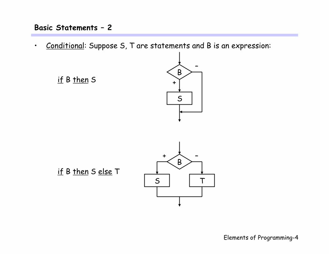
• Conditional: Suppose S, T are statements and B is an expression:
if B then S
if B then S else T
+
–
S
B
+ –
T
B
S
Elements of Programming-5
Basic Statements – 3
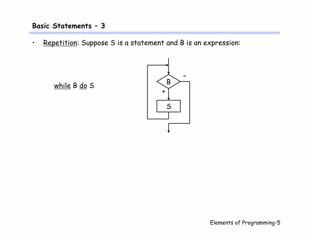
• Repetition: Suppose S is a statement and B is an expression:
while B do S
+
–
S
B
Elements of Programming-6
First Example
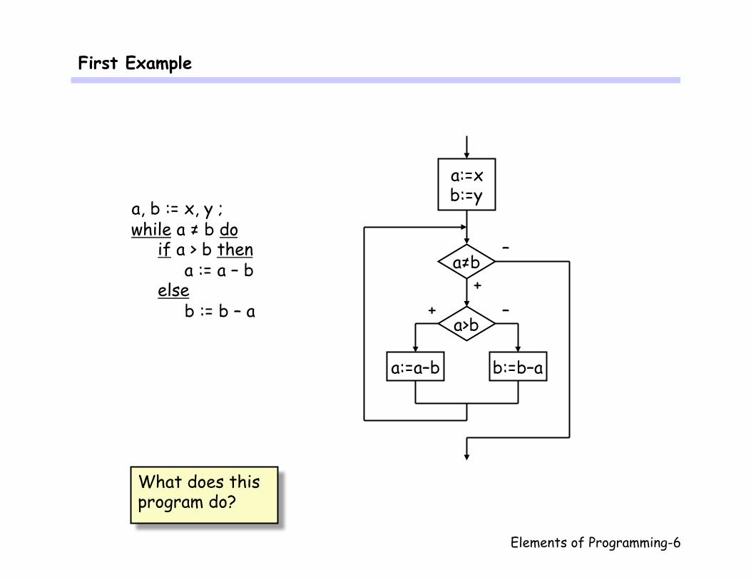
a, b := x, y ; while a ≠ b do if a > b then a := a – b else b := b – a
+
– a≠b
+ –
b:=b–a
a>b
a:=a–b
a:=x b:=y
What does this program do?

Elements of Programming-7
Properties of Statements
• Of the various properties of a statements (like code size, running time, memory used) we are interested in its interpretation as transforming values of variables. For example, if initially x = 3 then after y := x + 2 we have finally y = 5.
• However, we are more interested in properties holding for every
execution rather than for individual executions. We express such properties by predicates (boolean expressions) in the initial and final states. For example, if initially x ≥ a then after x := x + 1 we have finally x ≥ a + 1.

Elements of Programming-8
Correctness Assertions
• For statement S and predicates P, Q, we express that under precondition P program S will establish postcondition Q by the correctness assertion:
{P} S {Q}
• Examples (all variables are integers): {x = 3} y := x + 2 {y = 5}
{x ≥ a} x := x + 1 {x ≥ a + 1}
• Correctness assertions were introduced by C. A. R. Hoare in 1969. We also say that S is correct with respect to precondition P and postcondition Q.
S
P
Q
y := x + 2 x = 3
y = 5
x := x + 1 x ≥ a
x ≥ a + 1

Elements of Programming-9
Examples of Correctness Assertions
• {true} y := x + 2 {y = x + 2}
• {x = a - 3} x := x + 3 {x = a}
• {(z + u · y = a) ∧ (u > 0)} z, u := z + y, u – 1 {(z + u · y = a) ∧ (u ≥ 0)}
• Let gcd(x, y) be the greatest common divisor of integers x and y: {(x > 0) ∧ (y > 0)} a, b := x, y ; while a ≠ b do
if a > b then a := a – b else b := b – a {a = b = gcd(x, y)}

Elements of Programming-10
Program Annotations
• We can subdivide the task of checking correctness assertions by adding intermediate annotations: {x ≥ 0} z, u := 0, x ; {invariant: (z + u · y = x · y) ∧ (u ≥ 0)} while u > 0 do
z, u := z + y, u – 1 {z = x · y}
z := 0 u := x
u > 0
z := z + y u := u – 1
(z + u · y = x · y) ∧ (u ≥ 0)
x ≥ 0
z = x · y
+
–
Elements of Programming-11
Graphical Rules for Checking Annotations
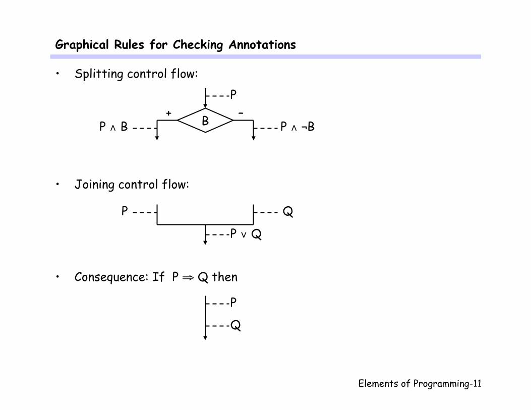
• Splitting control flow:
• Joining control flow:
• Consequence: If P ⇒ Q then
B
P
P ∧ ¬B P ∧ B
Q P
P ∨ Q
P
Q
+ –
Elements of Programming-12
Describing Syntax – 1
• Let us make things more precise, starting with the syntax of programs.
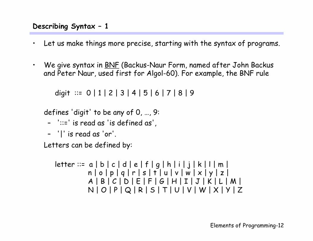
• We give syntax in BNF (Backus-Naur Form, named after John Backus and Peter Naur, used first for Algol-60). For example, the BNF rule digit ::= 0 | 1 | 2 | � 3 | 4 | 5 | 6 | 7 | 8 | 9 defines 'digit' to be any of 0, …, 9:
– '::=' is read as 'is defined as', – '|' is read as 'or'.
Letters can be defined by: letter ::= a | b | c | d | e | f | g | h | i | j | k | l | m |
n | o | p | q | r | s | t | u | v | w | x | y | z | A | B | C | D | E | F | G | H | I | J | K | L | M | N | O | P | Q | R | S | T | U | V | W | X | Y | Z
Elements of Programming-13
Describing Syntax – 2
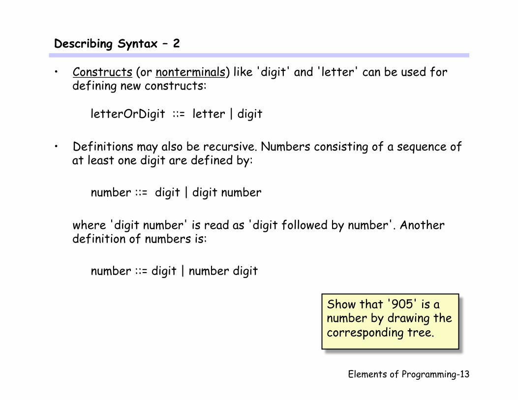
• Constructs (or nonterminals) like 'digit' and 'letter' can be used for defining new constructs:
letterOrDigit ::= letter | digit
• Definitions may also be recursive. Numbers consisting of a sequence of at least one digit are defined by: number ::= digit | digit number where 'digit number' is read as 'digit followed by number'. Another definition of numbers is: number ::= digit | number digit
Show that '905' is a number by drawing the corresponding tree.

Elements of Programming-14
Describing Syntax – 3
• Identifiers are defined as a sequence of letter and digits, starting with a letter: identifier ::= letter | identifier letterOrDigit Examples of identifiers: max U2 g q2p9 Brrrr Examples of that are not identifiers: P.Miller read-write 3d
Argue why these character sequences are identifiers or not.

Elements of Programming-15
Syntax of Statements …
• We define the statements of our design notation by following rules: statement ::= identifierList := expressionList
| begin statementSequence end | if expression then statement | if expression then statement else statement | while expression do statement
identifierList ::= identifier | identifierList , identifier expressionList ::= expression | expressionList , expression statementSequence ::= statement
| statementSequence ; statement
• Keywords like if and while are underlined to express that they are single symbols and not character sequences forming an identifier. Hence they are excluded from the set of identifiers.

Elements of Programming-16
… Syntax of Statements
• In assignments identifierList and expressionList must be of equal length and all identifiers must be distinct.
• Note that 'command' or 'instruction' would be a better term than 'statement' since a 'statement' does not state anything. As it is used in Pascal, C, C++, Java, 'statement' has become the common term.
• Examples of statements: – a, b := 7, 8 – begin a := 7 ; begin b := 8 ; c := 9 end end – if a > b then while a > 0 do a := a – 1 else b := 7
• Examples that are not statements:
– a := 3; – if a > b then a := a – b end – if b = 7 then a := 0 ; b := 9 else b := a – begin a := a + b, b := b – 1 end
Argue why these are statements or not.
Elements of Programming-17
Nested Conditionals …
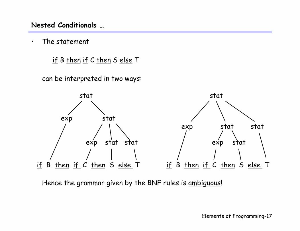
• The statement if B then if C then S else T can be interpreted in two ways:
Hence the grammar given by the BNF rules is ambiguous!
exp
exp stat stat
exp
exp stat
stat stat
stat
stat
stat
if B then if C then S else T if B then if C then S else T
Elements of Programming-18
… Nested Conditionals
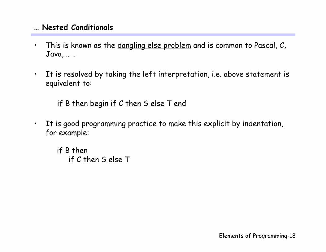
• This is known as the dangling else problem and is common to Pascal, C, Java, … .
• It is resolved by taking the left interpretation, i.e. above statement is equivalent to: if B then begin if C then S else T end
• It is good programming practice to make this explicit by indentation, for example:
if B then if C then S else T
Elements of Programming-19
Expressions
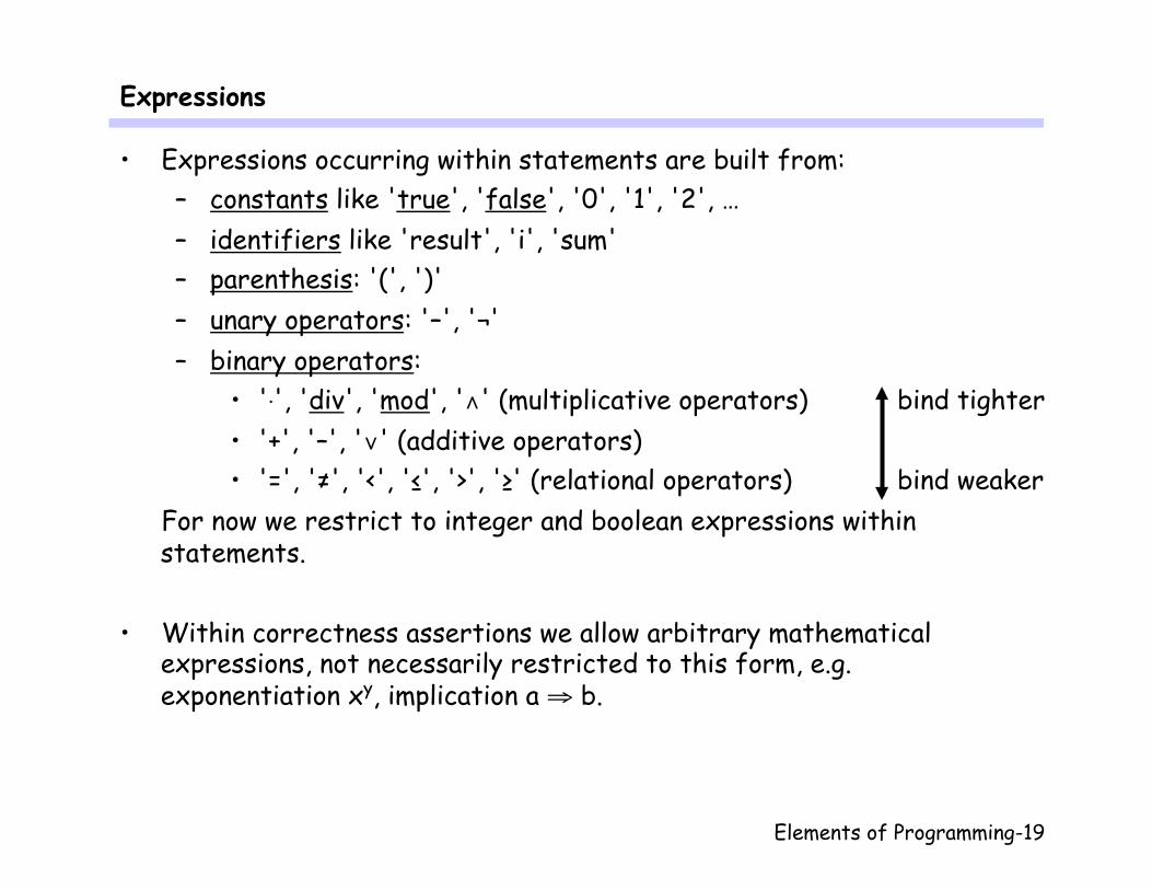
• Expressions occurring within statements are built from: – constants like 'true', 'false', '0', '1', '2', … – identifiers like 'result', 'i', 'sum' – parenthesis: '(', ')' – unary operators: '–', '¬' – binary operators:
• '·', 'div', 'mod', '∧' (multiplicative operators) bind tighter • '+', '–', '∨' (additive operators) • '=', '≠', '<', '≤', '>', '≥' (relational operators) bind weaker
For now we restrict to integer and boolean expressions within statements.
• Within correctness assertions we allow arbitrary mathematical
expressions, not necessarily restricted to this form, e.g. exponentiation xy, implication a ⇒ b.

Elements of Programming-20
Syntax of Expressions …
• We define the syntax of expressions recursively: factor ::= number
| false | true | identifier | ( expression ) | unaryOperator factor
term ::= factor | term mulOperator factor
unaryOperator ::= – | ¬
mulOperator ::= · | div | mod | ∧
Is x · y div 2 interpreted as – (x · y) div 2 or - x · (y div 2) ?
Elements of Programming-21
… Syntax of Expressions
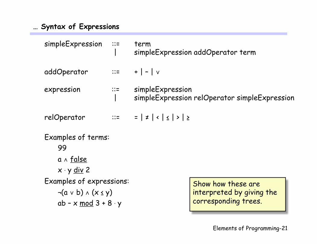
simpleExpression ::= term | simpleExpression addOperator term
addOperator ::= + | – | ∨ expression ::= simpleExpression
| simpleExpression relOperator simpleExpression relOperator ::= = | ≠ | < | ≤ | > �| ≥ Examples of terms:
99 a ∧ false x · y div 2
Examples of expressions: ¬(a ∨ b) ∧ (x ≤ y) ab – x mod 3 + 8 · y
Show how these are interpreted by giving the corresponding trees.
Elements of Programming-22
Types
• In order to disallow expressions like 'a + true', we assign each expression (in statements and in assertions) a unique type.
• We distinguish basic types and composed types. – Fundamental basic types are integer (Z) and boolean. (To those we
add real (R), char, …, as needed). – Fundamental composed types are product types and function types.
• We express that expression E is of type T as E : T, e.g.
x : integer (y + 3) : integer x = y : boolean ¬(a ∧ b) : boolean
Elements of Programming-23
Product and Function Types
• If T1, …, Tn are types, then T1 × … × Tn is a product type. For example: – (2, 'm', 'e', 3) : integer × char × char × integer – (3, ('a', true)) : integer × (char × boolean)
• If T, U are types, then T → U is a function type. For example: – sin : real → real – power : real × integer → real – + : integer × integer → integer – + : real × real → real
Note that – binary operators are just functions written in infix form, i.e. x + y
stands for +(x, y); – it is common practice to overload functions, e.g. + stands for
addition of integers or reals or matrices etc. Which one it stands for must be inferred from the context;
– If f : T → U and a : T then f a : U, also written f(a) : U. For example if (a + b) : real then sin(a + b) : real.

Elements of Programming-24
Checking Types
• For any type T, we have = : T × T → boolean
• Examples: Well-typed expressions: a ∧ b = (x > y) provided a, b : boolean and x, y : integer a mod b div c provided a, b, c : integer
Syntactically correct but not well-typed expressions: true = 1 a = 0 ∧ b
• Remark: if we would have only integer and boolean, we could change the syntax to allow only well-typed expressions. However, as soon as we allow composed types (like arrays of arrays of records) we can no longer express correct typing in BNF. Both syntax and typing is checked by compilers, though all modern programming languages define syntax only in BNF and typing separately.
Show this!
Elements of Programming-25
The Type integer
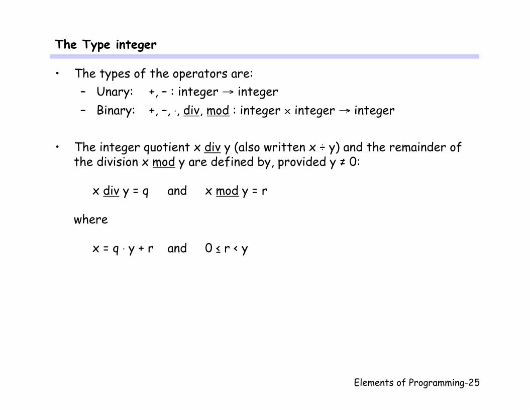
• The types of the operators are: – Unary: +, – : integer → integer – Binary: +, –, ·, div, mod : integer × integer → integer
• The integer quotient x div y (also written x ÷ y) and the remainder of the division x mod y are defined by, provided y ≠ 0:
x div y = q and x mod y = r where
x = q · y + r and 0 ≤ r < y
Elements of Programming-26
The Type boolean
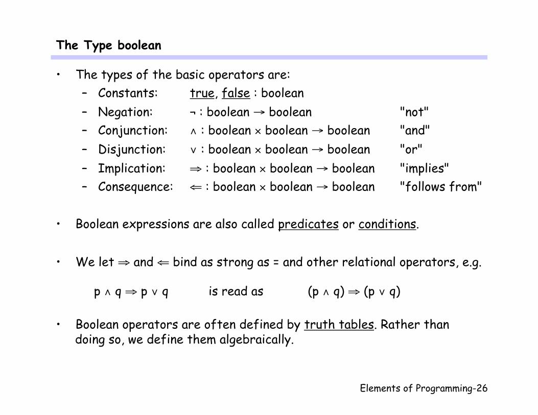
• The types of the basic operators are: – Constants: true, false : boolean – Negation: ¬ : boolean → boolean "not" – Conjunction: ∧ : boolean × boolean → boolean "and" – Disjunction: ∨ : boolean × boolean → boolean "or" – Implication: ⇒ : boolean × boolean → boolean "implies" – Consequence: ⇐ : boolean × boolean → boolean "follows from"
• Boolean expressions are also called predicates or conditions.
• We let ⇒ and ⇐ bind as strong as = and other relational operators, e.g.
p ∧ q ⇒ p ∨ q is read as (p ∧ q) ⇒ (p ∨ q)
• Boolean operators are often defined by truth tables. Rather than doing so, we define them algebraically.
Elements of Programming-27
Boolean Algebra
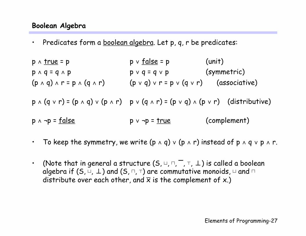
• Predicates form a boolean algebra. Let p, q, r be predicates:
p ∧ true = p p ∨ false = p (unit) p ∧ q = q ∧ p p ∨ q = q ∨ p ��������� (symmetric) (p ∧ q) ∧ r = p ∧ (q ∧ r) (p ∨ q) ∨ r = p ∨ (q ∨ r) (associative)
p ∧ (q ∨ r) = (p ∧ q) ∨ (p ∧ r) p ∨ (q ∧ r) = (p ∨ q) ∧ (p ∨ r) (distributive)
p ∧ ¬p = false p ∨ ¬p = true (complement) • To keep the symmetry, we write (p ∧ q) ∨ (p ∧ r) instead of p ∧ q ∨ p ∧ r.
• (Note that in general a structure (S, ⊔, ⊓, ‾, ⊤, ⊥) is called a boolean algebra if (S, ⊔, ⊥) and (S, ⊓, ⊤) are commutative monoids, ⊔ and ⊓ distribute over each other, and x ̅ is the complement of x.)
Elements of Programming-28
Theorems of Boolean Algebra
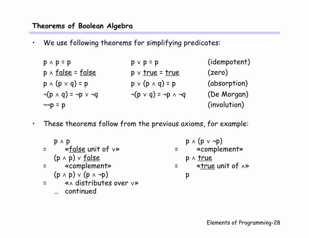
• We use following theorems for simplifying predicates: p ∧ p = p p ∨ p = p (idempotent) p ∧ false = false p ∨ true = true (zero) p ∧ (p ∨ q) = p p ∨ (p ∧ q) = p (absorption) ¬(p ∧ q) = ¬p ∨ ¬q ¬(p ∨ q) = ¬p ∧ ¬q (De Morgan) ¬¬p = p (involution)
• These theorems follow from the previous axioms, for example:
p ∧ p p ∧ (p ∨ ¬p) = «false unit of ∨» = «complement»
(p ∧ p) ∨ false p ∧ true = «complement» = «true unit of ∧»
(p ∧ p) ∨ (p ∧ ¬p) p = «∧ distributes over ∨»
… continued
Elements of Programming-29
Ordering of Predicates …
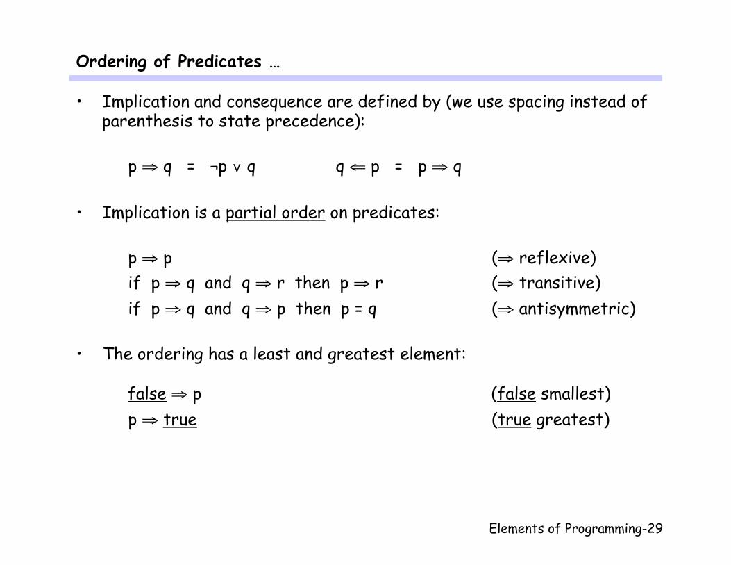
• Implication and consequence are defined by (we use spacing instead of parenthesis to state precedence): p ⇒ q = ¬p ∨ q q ⇐ p = p ⇒ q
• Implication is a partial order on predicates: p ⇒ p (⇒ reflexive) if p ⇒ q and q ⇒ r then p ⇒ r (⇒ transitive) if p ⇒ q and q ⇒ p then p = q (⇒ antisymmetric)
• The ordering has a least and greatest element:
false ⇒ p (false smallest) p ⇒ true (true greatest)

Elements of Programming-30
… Ordering of Predicates
• Conjunction gives the greatest lower bound:
p ∧ q ⇒ p (weakening / strengthening) if r ⇒ p and r ⇒ q then r ⇒ p ∧ q Dually, disjunction gives the least upper bound:
p ⇒ p ∨ q (weakening / strengthening) if p ⇒ r and q ⇒ r then p ∨ q ⇒ r
• Conjunction and disjunction are monotonic, negation is antimonotonic:
if p ⇒ q then p ∧ r ⇒ q ∧ r (∧ monotonic) if p ⇒ q then p ∨ r ⇒ q ∨ r (∨ monotonic) if p ⇒ q then ¬q ⇒ ¬p (¬ antimonotonic)
• We read 'p ⇒ q' also as 'p less than q' or 'p is stronger than q' or 'q is weaker than p'.
Elements of Programming-31
Substitution
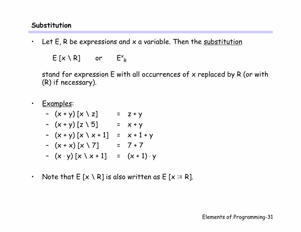
• Let E, R be expressions and x a variable. Then the substitution
E [x \ R] or ExR
stand for expression E with all occurrences of x replaced by R (or with (R) if necessary).
• Examples: – (x + y) [x \ z] = z + y – (x + y) [z \ 5] = x + y – (x + y) [x \ x + 1] = x + 1 + y – (x + x) [x \ 7] = 7 + 7 – (x · y) [x \ x + 1] = (x + 1) · y
• Note that E [x \ R] is also written as E [x := R].
Elements of Programming-32
Multiple Substitutions
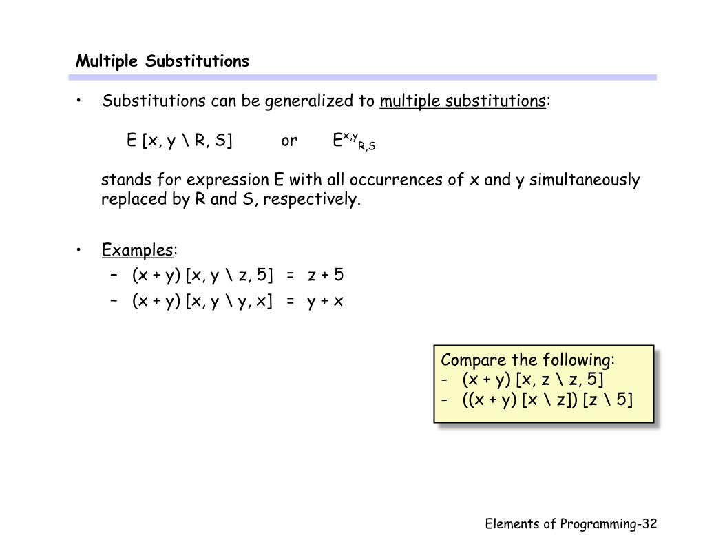
• Substitutions can be generalized to multiple substitutions:
E [x, y \ R, S] or Ex,yR,S
stands for expression E with all occurrences of x and y simultaneously replaced by R and S, respectively.
• Examples: – (x + y) [x, y \ z, 5] = z + 5 – (x + y) [x, y \ y, x] = y + x
Compare the following: - (x + y) [x, z \ z, 5] - ((x + y) [x \ z]) [z \ 5]

Elements of Programming-33
Equality and Proofs …
• Equality is reflexive, transitive, and symmetric: E = E (= reflexive) if E = F and F = G then E = G (= transitive) if E = F then F = E (= symmetric) For example, in the proof on slide 28 transitivity was used silently.
• Equals can be replaced by equals:
if E = F then G [x \ E] = G [x \ F] (Leibniz)
• Stating (or proving) that E is equal to true means stating E:
(E = true) = E
Elements of Programming-34
… Equality and Proofs
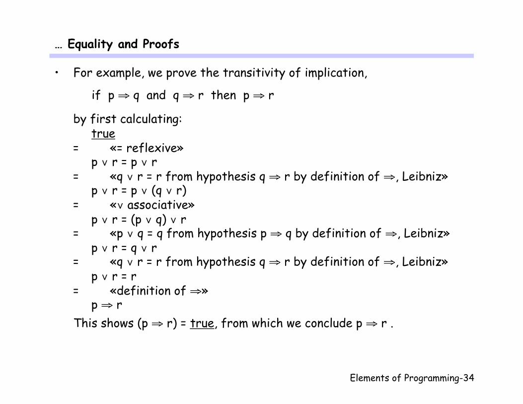
• For example, we prove the transitivity of implication,
if p ⇒ q and q ⇒ r then p ⇒ r
by first calculating: true
= «= reflexive» p ∨ r = p ∨ r
= «q ∨ r = r from hypothesis q ⇒ r by definition of ⇒, Leibniz» p ∨ r = p ∨ (q ∨ r)
= «∨ associative» p ∨ r = (p ∨ q) ∨ r
= «p ∨ q = q from hypothesis p ⇒ q by definition of ⇒, Leibniz» p ∨ r = q ∨ r
= «q ∨ r = r from hypothesis q ⇒ r by definition of ⇒, Leibniz» p ∨ r = r
= «definition of ⇒» p ⇒ r
This shows (p ⇒ r) = true, from which we conclude p ⇒ r .

Elements of Programming-35
Weakest Preconditions
• All of the following correctness assertions hold: {x ≥ 4} x := x + 1 {x ≥ 3} {x ≥ 3} x := x + 1 {x ≥ 3} {x ≥ 2} x := x + 1 {x ≥ 3}
However, among those the last one is the strongest claim: x ≥ 2 is the weakest precondition for x := x + 1 to establish x ≥ 3.
• The weakest precondition such that statement S establishes postcondition R is written as:
wp(S, R) For example:
(x ≥ 2) = wp(x := x + 1, x ≥ 3) As we are only interested in the input-output behavior of statements, we can define them completely through wp.

Elements of Programming-36
Definition of Assignment
• wp(x := E, P) = P [x \ E] wp(x, y := E, F, P) = P [x, y \ E, F]
• Examples: wp(y := x + 2, y = x + 2) = «wp of assignment»
(y = x + 2) [y \ x + 2] = «substitution»
x + 2 = x + 2 = «logic (as E = E and E = (E = true) for any E)»
true wp(x := x + y, x > y) = «wp of assignment»
(x > y) [x \ x + y] = «substitution»
x + y > y = «arithmetic»
x > 0

Elements of Programming-37
Definition of Sequential Composition and Compound Statement
• wp(S ; T, R) = wp(S, wp(T, R)) wp(begin S end, R) = wp(S, R)
• Example: wp(y := y – z ; y := y · y, y < 4) = «wp of sequential composition»
wp(y := y – z, wp(y := y · y, y < 4)) = «wp of assignment, substitution»
wp(y := y – z, y · y < 4) = «wp of assignment, substitution»
(y – z) · (y – z) < 4 = «arithmetic»
–2 < y – z < 2 Note that E < F < G stands for (E < F) ∧ (F < G).

Elements of Programming-38
Definition of Conditionals
• wp(if B then S, R) = (B ⇒ wp(S, R)) ∧ (¬B ⇒ R) wp(if B then S else T, R) = (B ⇒ wp(S, R)) ∧ (¬B ⇒ wp(T, R))
• Example:
wp(if x < 0 then x := – x, x ≥ 0) = «wp of if-then»
((x < 0) ∧ wp(x := – x, x ≥ 0)) ∨ (¬(x < 0) ∧ (x ≥ 0)) = «wp of assignment, arithmetic»
((x < 0) ∧ (x ≥ 0) [x \ – x]) ∨ (x ≥ 0) = «substitution»
((x < 0) ∧ (– x ≥ 0)) ∨ (x ≥ 0) = «arithmetic ((-x ≥ 0) = (x ≤ 0) = (x < 0) ∨ (x = 0))»
(x < 0) ∨ (x ≥ 0) = «arithmetic»
true
Elements of Programming-39
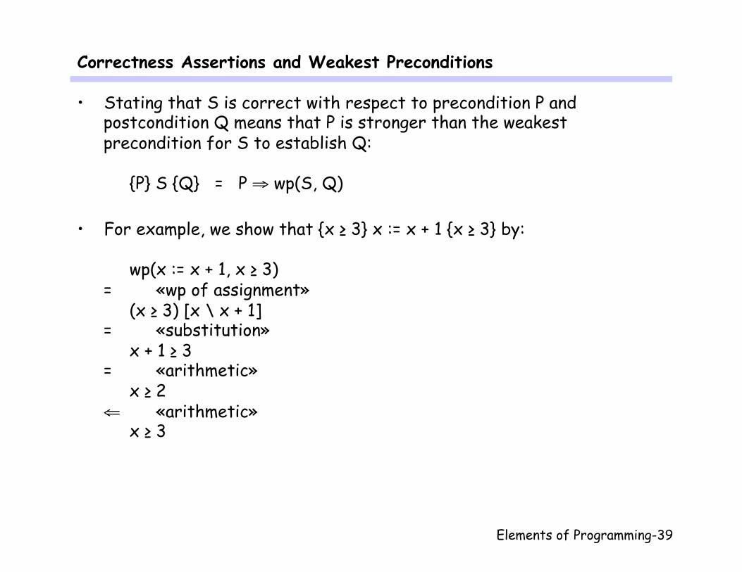
Correctness Assertions and Weakest Preconditions
• Stating that S is correct with respect to precondition P and postcondition Q means that P is stronger than the weakest precondition for S to establish Q:
{P} S {Q} = P ⇒ wp(S, Q)
• For example, we show that {x ≥ 3} x := x + 1 {x ≥ 3} by:
wp(x := x + 1, x ≥ 3) = «wp of assignment»
(x ≥ 3) [x \ x + 1] = «substitution»
x + 1 ≥ 3 = «arithmetic»
x ≥ 2 ⇐ «arithmetic»
x ≥ 3
Elements of Programming-40
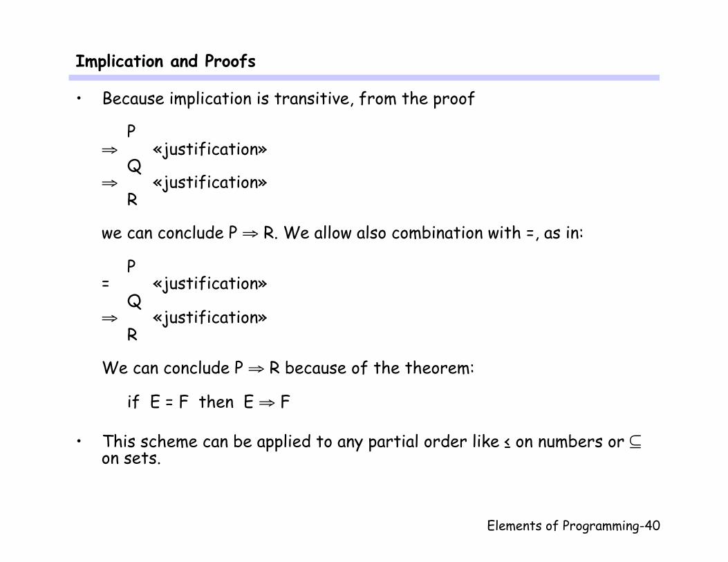
Implication and Proofs
• Because implication is transitive, from the proof
P ⇒ «justification»
Q ⇒ «justification»
R we can conclude P ⇒ R. We allow also combination with =, as in:
P = «justification»
Q ⇒ «justification»
R We can conclude P ⇒ R because of the theorem:
if E = F then E ⇒ F
• This scheme can be applied to any partial order like ≤ on numbers or ⊆ on sets.
Elements of Programming-41
Monotonicity of wp
• A stronger (weaker) postcondition leads to a stronger (weaker) precondition:
if P ⇒ Q then wp(S, P) ⇒ wp(S, Q) (This theorem can be proved by induction over the structure of statements.)
• Example:
wp(S, x > 5) ⇒ wp(S, x > 3)
• Consequences:
if P ⇒ wp(S, Q) and Q ⇒ R then P ⇒ wp(S, R) if P ⇒ wp(S, Q) and Q ⇒ wp(T, R) then P ⇒ wp(S ; T, R)
Reformulate the consequences with correctness assertions!
Elements of Programming-42
Conjunctivity of wp
• If we show that a statement establishes two postconditions, it also establishes their conjunction:
wp(S, P) ∧ wp(S, Q) = wp(S, P ∧ Q)
• Example: wp(x := 2 · x, (x ≥ 0) ∧ even(x))
= «conjunctivity of wp» wp(x := 2 · x, x ≥ 0) ∧ wp(x := 2 · x, even(x))
= «wp of assignment, substitution» (2 · x ≥ 0) ∧ even(2 · x)
= «arithmetic» x ≥ 0
• Consequence:
if P ⇒ wp(S, Q) and P ⇒ wp(S, R) then P ⇒ wp(S, Q ∧ R)

Elements of Programming-43
Rule for Repetition
• Rather than giving the exact weakest precondition, we give the main theorem about repetitions. Let – P be a predicate, the invariant; – T be an integer expression, the bound (or variant); – v be an auxiliary integer variable.
If B ∧ P ⇒ wp(S, P) (P is invariant of S) B ∧ P ∧ (T = v) ⇒ wp(S, T < v) (S decreases T) B ∧ P ⇒ T > 0 (T ≤ 0 causes termination) then
P ⇒ wp(while B do S, P ∧ ¬B) (The proof of this theorem requires a definition of loops that is outside of the scope of this course.)
Elements of Programming-44
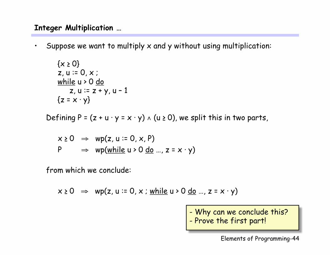
Integer Multiplication …
• Suppose we want to multiply x and y without using multiplication:
{x ≥ 0} z, u := 0, x ; while u > 0 do z, u := z + y, u – 1 {z = x · y}
Defining P = (z + u · y = x · y) ∧ (u ≥ 0), we split this in two parts, x ≥ 0 ⇒ wp(z, u := 0, x, P) P ⇒ wp(while u > 0 do …, z = x · y) from which we conclude: x ≥ 0 ⇒ wp(z, u := 0, x ; while u > 0 do …, z = x · y)
- Why can we conclude this? - Prove the first part!

Elements of Programming-45
… Integer Multiplication
• We now prove the second part using P as invariant and u as bound. As
(u > 0) ∧ P ⇒ wp(z, u := z + y, u – 1, P) (u > 0) ∧ P ∧ (u = v) ⇒ wp(z, u := z + y, u – 1, u < v) (u > 0) ∧ P ⇒ u > 0
we can conclude by the repetition rule P ⇒ wp(while u > 0 do z, u := z + y, u – 1, P ∧ ¬(u > 0)) from which we finally conclude (as u ≥ 0 and u ≤ 0 implies u = 0):
P ⇒ wp(while u > 0 do z, u := z + y, u – 1, z = x · y)
Prove these!
Elements of Programming-46
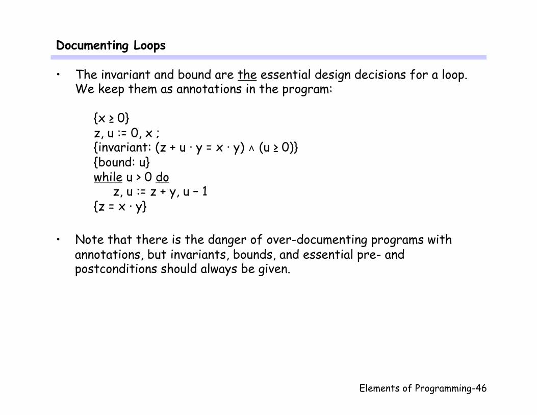
Documenting Loops
• The invariant and bound are the essential design decisions for a loop. We keep them as annotations in the program:
{x ≥ 0} z, u := 0, x ; {invariant: (z + u · y = x · y) ∧ (u ≥ 0)} {bound: u} while u > 0 do z, u := z + y, u – 1 {z = x · y}
• Note that there is the danger of over-documenting programs with
annotations, but invariants, bounds, and essential pre- and postconditions should always be given.
Elements of Programming-47
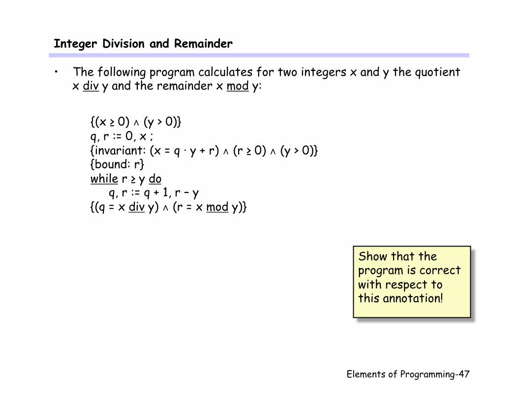
Integer Division and Remainder
• The following program calculates for two integers x and y the quotient x div y and the remainder x mod y:
{(x ≥ 0) ∧ (y > 0)} q, r := 0, x ; {invariant: (x = q · y + r) ∧ (r ≥ 0) ∧ (y > 0)} {bound: r} while r ≥ y do q, r := q + 1, r – y {(q = x div y) ∧ (r = x mod y)}
Show that the program is correct with respect to this annotation!

Elements of Programming-48
Euclids Algorithm
• The following program calculates for two integers x and y their greatest common divisor gcd(x, y).
{(x > 0) ∧ (y > 0)} a, b := x, y ; {invariant: (gcd(a, b) = gcd(x, y)) ∧ (a > 0) ∧ (b > 0)} {bound: a + b} while a ≠ b do if a > b then a := a – b else b := b – a {a = gcd(x, y)}
• We have following theorems about gcd:
gcd(x, y) = gcd(x – y, y) gcd(x, y) = gcd(y, x) gcd(x, x) = x

Elements of Programming-49
Arrays …
• Arrays are like sequences, except that an array variable cannot change its length. We write the type of an array as
array N of T for constant N and selecting an array element by a(E) (or a[E]). The alter function (a ; E : F) modifies a(E) to be F.
• For example, if a : array 4 of integer and a = 〈9, 3, 6, 7〉, then:
a(0) = 9 (a ; 1 : 11) = 〈9, 11, 6, 7〉 a(2) = 6 ((a ; 0 : 3) ; 1 : 8) = 〈3, 8, 6, 7〉 (a ; 0 : 8) = 〈8, 3, 6, 7〉 ((a ; 3 : 9) ; 3 : 8) = 〈9, 3, 6, 8〉
• Formally, the alter function (a; E: F) is defined recursively by:
if E = G then (a ; E : F)(G) = F if E ≠ G then (a ; E : F)(G) = a(G)
Elements of Programming-50
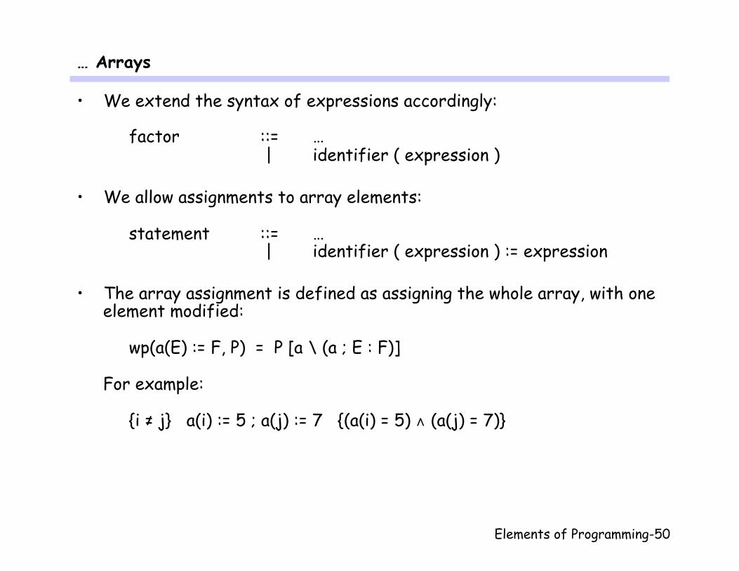
… Arrays
• We extend the syntax of expressions accordingly:
factor ::= … | identifier ( expression )
• We allow assignments to array elements:
statement ::= … | identifier ( expression ) := expression
• The array assignment is defined as assigning the whole array, with one
element modified:
wp(a(E) := F, P) = P [a \ (a ; E : F)] For example:
{i ≠ j} a(i) := 5 ; a(j) := 7 {(a(i) = 5) ∧ (a(j) = 7)}
Elements of Programming-51
Sum of Array Elements
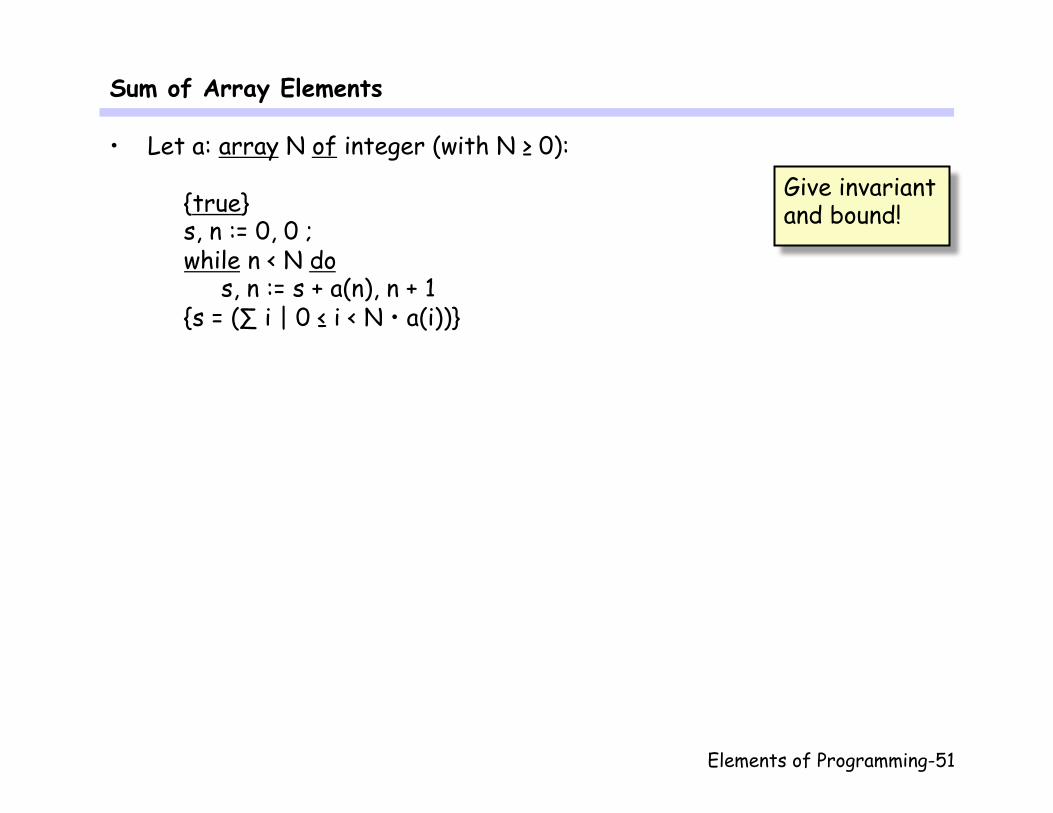
• Let a: array N of integer (with N ≥ 0):
{true} s, n := 0, 0 ; while n < N do s, n := s + a(n), n + 1 {s = (∑ i | 0 ≤ i < N • a(i))}
Give invariant and bound!

Elements of Programming-52
Vector Addition
• Let a, b, c : array N of integer represent three vectors: {N ≥ 0}
n := 0 ; {invariant: (∀ i | 0 ≤ i < n • c(i) = a(i) + b(i)) ∧ (0 ≤ n ≤ N)} {bound: N – n} while n < N do begin c(n) := a(n) + b(n) ; n := n + 1 end {(∀ i | 0 ≤ i < N • c(i) = a(i) + b(i))}
Note that the postcondition can be more briefly written as:
c = a + b

Elements of Programming-53
Multi-Dimensional Arrays
• For multi-dimensional arrays we use:
array M, N of T for array M of array N of T a(E, F) for a(E)(F)
• The array assignment is defined as assigning the whole array, with one element modified:
wp(a(E, F) := G, P) = P [a \ (a ; E : (a(E) ; F : G))] For example:
{true} a(i, j) := a(j, i) {a(i, j) = a(j, i)}
Elements of Programming-54
Matrix Multiplication …
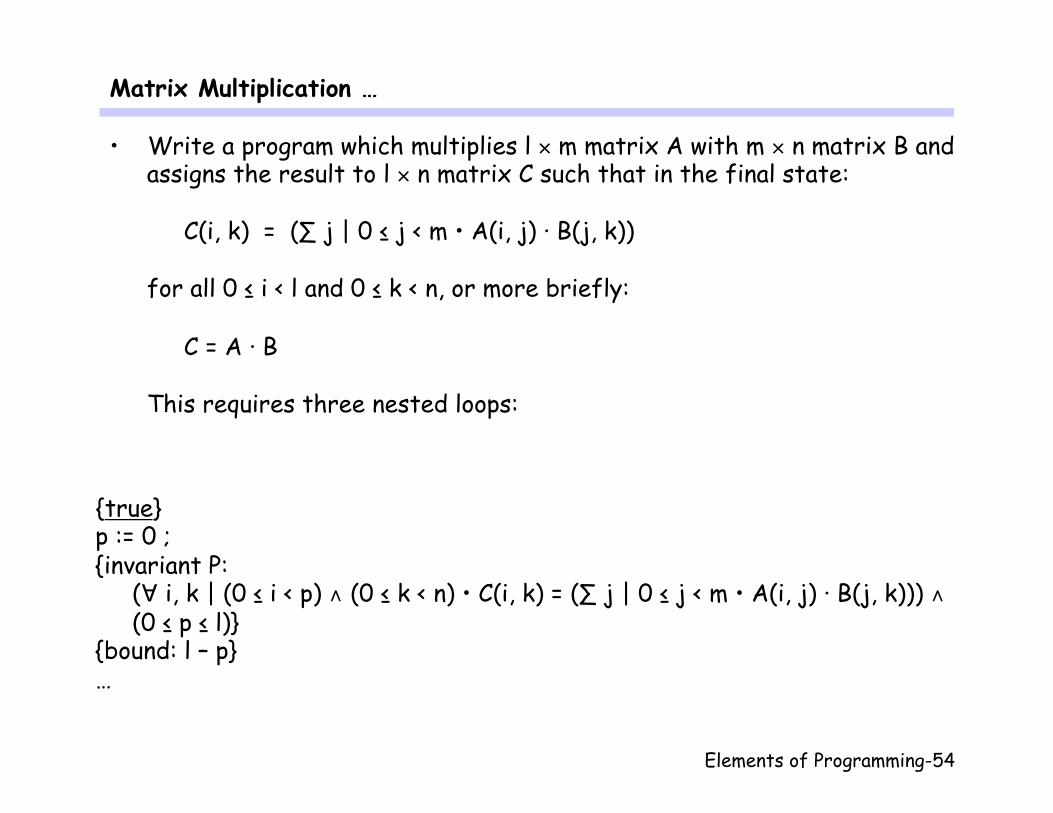
• Write a program which multiplies l × m matrix A with m × n matrix B and assigns the result to l × n matrix C such that in the final state:
C(i, k) = (∑ j | 0 ≤ j < m • A(i, j) · B(j, k)) for all 0 ≤ i < l and 0 ≤ k < n, or more briefly:
C = A · B This requires three nested loops:
{true} p := 0 ; {invariant P:
(∀ i, k | (0 ≤ i < p) ∧ (0 ≤ k < n) • C(i, k) = (∑ j | 0 ≤ j < m • A(i, j) · B(j, k))) ∧ (0 ≤ p ≤ l)}
{bound: l – p} …

Elements of Programming-55
… Matrix Multiplication
while p < l do begin q := 0 ; {invariant Q: P ∧ (∀ k | 0 ≤ k < q • C(p, k) = (∑ j | 0 ≤ j < m • A(p, j) · B(j, k))) ∧ (0 ≤ q ≤ n)} {bound: n – q} while q < n do begin r := 0 ; C(p, q) := 0 ; {invariant R: Q ∧ (C(p, q) = (∑ j | 0 ≤ j < r • A(p, j) · B(j, q))) ∧ (0 ≤ r ≤ m)} {bound: m – r} while r < m do begin C(p, q) := C(p, q) + A(p, r) · B(r, q) ; r := r + 1 end ; q := q + 1 end ; p := p + 1 end
{(∀ i, k | (0 ≤ i < l) ∧ (0 ≤ k < n) • C(i, k) = (∑ j | 0 ≤ j < m • A(i, j) · B(j, k)))}
Elements of Programming-56
Quantification
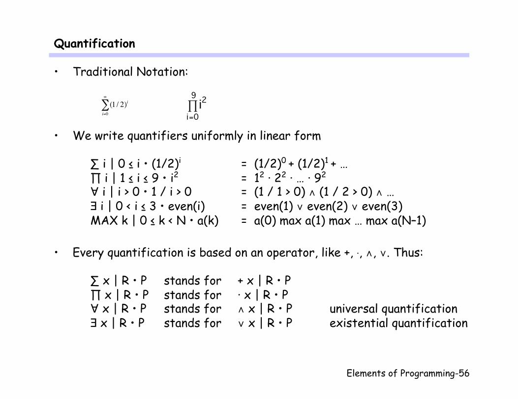
• Traditional Notation:
• We write quantifiers uniformly in linear form
∑ i | 0 ≤ i • (1/2)i = (1/2)0 + (1/2)1 + … ∏ i | 1 ≤ i ≤ 9 • i2 = 12 · 22 · … · 92 ∀ i | i > 0 • 1 / i > 0 = (1 / 1 > 0) ∧ (1 / 2 > 0) ∧ … ∃ i | 0 < i ≤ 3 • even(i) = even(1) ∨ even(2) ∨ even(3) MAX k | 0 ≤ k < N • a(k) = a(0) max a(1) max … max a(N–1)
• Every quantification is based on an operator, like +, ·, ∧, ∨. Thus:
∑ x | R • P stands for + x | R • P ∏ x | R • P stands for · x | R • P ∀ x | R • P stands for ∧ x | R • P universal quantification ∃ x | R • P stands for ∨ x | R • P existential quantification
(1 / 2)ii=0
∞
∑
i2i=0
9∏

Elements of Programming-57
Syntax of Quantification
• General form of quantification is * x : T | P • E where: – * is a symmetric, associative operator with identity. – x is the bound variable of the quantification; there may be several
bound variables. – T is the type of the bound variable; if it is understood from the
context, it is usually omitted. – P a predicate, the range of the quantification. – E is an expression, the body of the quantification.
• For predicates, the range is optional as:
(∀ x | P • Q) = (∀ x • P ⇒ Q) (trading) (∃ x | P • Q) = (∃ x • P ∧ Q)
Elements of Programming-58
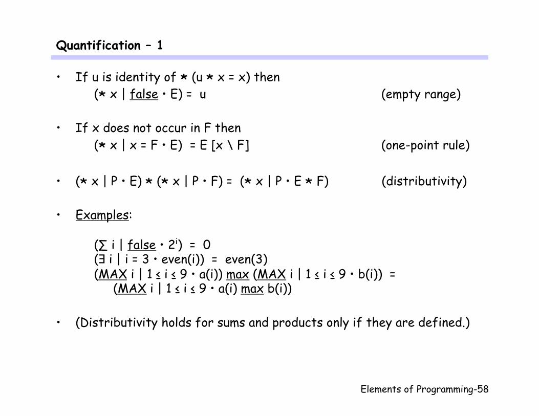
Quantification – 1
• If u is identity of * (u * x = x) then (* x | false • E) = u (empty range)
• If x does not occur in F then
(* x | x = F • E) = E [x \ F] (one-point rule)
• (* x | P • E) * (* x | P • F) = (* x | P • E * F) (distributivity)
• Examples:
(∑ i | false • 2i) = 0 (∃ i | i = 3 • even(i)) = even(3) (MAX i | 1 ≤ i ≤ 9 • a(i)) max (MAX i | 1 ≤ i ≤ 9 • b(i)) = (MAX i | 1 ≤ i ≤ 9 • a(i) max b(i))
• (Distributivity holds for sums and products only if they are defined.)
Elements of Programming-59
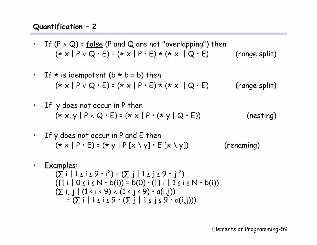
Quantification – 2
• If (P ∧ Q) = false (P and Q are not "overlapping") then (* x | P ∨ Q • E) = (* x | P • E) * (* x | Q • E) (range split)
• If * is idempotent (b * b = b) then
(* x | P ∨ Q • E) = (* x | P • E) * (* x | Q • E) (range split)
• If y does not occur in P then (* x, y | P ∧ Q • E) = (* x | P • (* y | Q • E)) (nesting)
• If y does not occur in P and E then
(* x | P • E) = (* y | P [x \ y] • E [x \ y]) (renaming)
• Examples: (∑ i | 1 ≤ i ≤ 9 • i2) = (∑ j | 1 ≤ j ≤ 9 • j 2) (∏ i | 0 ≤ i ≤ N • b(i)) = b(0) · (∏ i | 1 ≤ i ≤ N • b(i)) (∑ i, j | (1 ≤ i ≤ 9) ∧ (1 ≤ j ≤ 9) • a(i,j)) = (∑ i | 1 ≤ i ≤ 9 • (∑ j | 1 ≤ j ≤ 9 • a(i,j)))

Elements of Programming-60
Quantification and Substitution
• In the expression (∑ i | 1 ≤ i ≤ 9 • ij) + i · j – the occurrences of i in 1 ≤ i ≤ 9 and in ij are bound, – the occurrence of i in i · j is free – the occurrences of j in ij and i · j are free.
We say that variable x occurs in E if there is a free occurrence.
• If y does not occur in F (and is different from x) then (* y | P • E) [x \ F] = (* y | P [x \ F] • E [x \ F]) (substitution)
• Care has to be taken that a free variable cannot become bound by a substitution. For example:
(∑ b | 1 ≤ b ≤ 9 • ab) [a \ b] = «renaming»
(∑ c | 1 ≤ c ≤ 9 • ac) [a \ b] = «substitution»
(∑ c | 1 ≤ c ≤ 9 • bc)
Elements of Programming-61
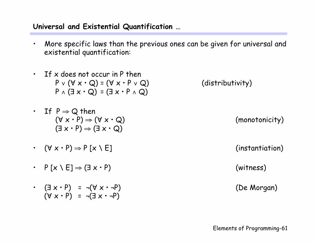
Universal and Existential Quantification …
• More specific laws than the previous ones can be given for universal and existential quantification:
• If x does not occur in P then P ∨ (∀ x • Q) = (∀ x • P ∨ Q) (distributivity) P ∧ (∃ x • Q) = (∃ x • P ∧ Q)
• If P ⇒ Q then
(∀ x • P) ⇒ (∀ x • Q) (monotonicity) (∃ x • P) ⇒ (∃ x • Q)
• (∀ x • P) ⇒ P [x \ E] (instantiation)
• P [x \ E] ⇒ (∃ x • P) (witness)
• (∃ x • P) = ¬(∀ x • ¬P) (De Morgan)
(∀ x • P) = ¬(∃ x • ¬P)

Elements of Programming-62
… Universal and Existential Quantification
• (∃ x • (∀ y • P)) ⇒ (∀ y • (∃ x • P)) (interchange)
• Example (from Slide 64, very detailed): Assume n does not occur in b(i)
(∀ i: integer | 0 ≤ i < n • ¬b(i)) [n \ n + 1] = «substitution, assumption»
(∀ i: integer | 0 ≤ i < n + 1 • ¬b(i)) = «arithmetic»
(∀ i: integer | (0 ≤ i < n) ∨ (i = n) • ¬b(i)) = «range split»
(∀ i: integer | 0 ≤ i < n • ¬b(i)) ∧ (∀ i: integer | i = n • ¬b(i)) = «one-point rule»
(∀ i: integer | 0 ≤ i < n • ¬b(i)) ∧ (¬b(i)) [ i \ n] = «substitution»
(∀ i: integer | 0 ≤ i < n • ¬b(i)) ∧ ¬b(n)
Elements of Programming-63
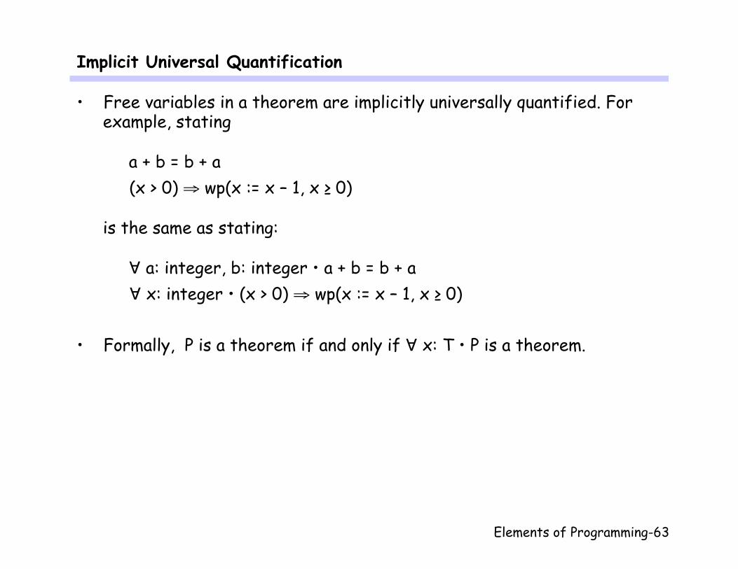
Implicit Universal Quantification
• Free variables in a theorem are implicitly universally quantified. For example, stating
a + b = b + a (x > 0) ⇒ wp(x := x – 1, x ≥ 0) is the same as stating:
∀ a: integer, b: integer • a + b = b + a ∀ x: integer • (x > 0) ⇒ wp(x := x – 1, x ≥ 0)
• Formally, P is a theorem if and only if ∀ x: T • P is a theorem.
Elements of Programming-64
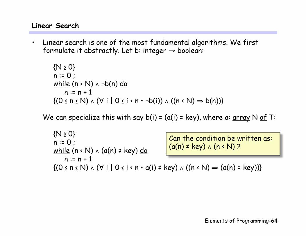
Linear Search
• Linear search is one of the most fundamental algorithms. We first formulate it abstractly. Let b: integer → boolean:
{N ≥ 0} n := 0 ; while (n < N) ∧ ¬b(n) do n := n + 1 {(0 ≤ n ≤ N) ∧ (∀ i | 0 ≤ i < n • ¬b(i)) ∧ ((n < N) ⇒ b(n))}
We can specialize this with say b(i) = (a(i) = key), where a: array N of T:
{N ≥ 0} n := 0 ; while (n < N) ∧ (a(n) ≠ key) do n := n + 1 {(0 ≤ n ≤ N) ∧ (∀ i | 0 ≤ i < n • a(i) ≠ key) ∧ ((n < N) ⇒ (a(n) = key))}
Can the condition be written as: (a(n) ≠ key) ∧ (n < N) ?

Elements of Programming-65
Partially Defined Expressions
• While mathematically every well-typed expression has a value, trying to evaluate certain expressions in a program is an error. For example,
x div y = x div y is true in mathematics (a consequence of = reflexive). However,
if x div y = x div y then x := 5 is not the same as
if true then x := 5 as the first may fail if y = 0 while the second will always terminate.
• We have to distinguish expressions by their definedness domain: x div y = x div y is defined only if y ≠ 0 true is always defined
Hence they are not "equal"!
Elements of Programming-66
Definedness Domain
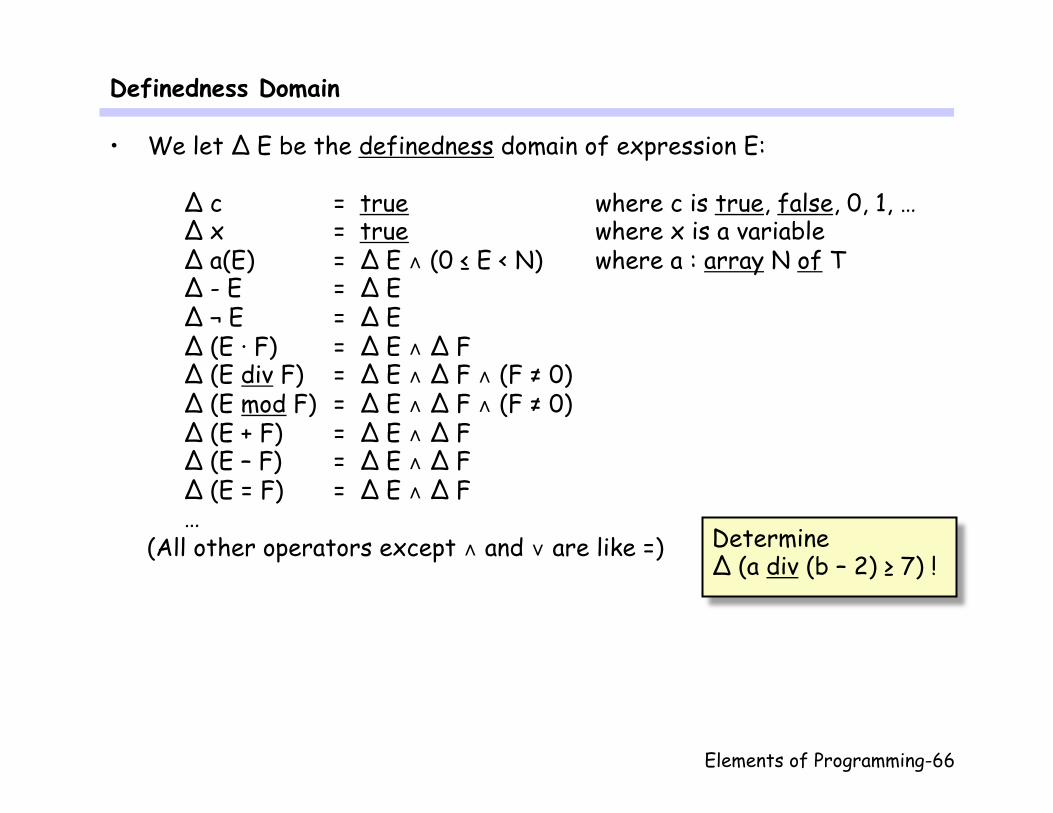
• We let ∆ E be the definedness domain of expression E:
∆ c = true where c is true, false, 0, 1, … ∆ x = true where x is a variable ∆ a(E) = ∆ E ∧ (0 ≤ E < N) where a : array N of T ∆ - E = ∆ E ∆ ¬ E = ∆ E ∆ (E · F) = ∆ E ∧ ∆ F ∆ (E div F) = ∆ E ∧ ∆ F ∧ (F ≠ 0) ∆ (E mod F) = ∆ E ∧ ∆ F ∧ (F ≠ 0) ∆ (E + F) = ∆ E ∧ ∆ F ∆ (E – F) = ∆ E ∧ ∆ F ∆ (E = F) = ∆ E ∧ ∆ F …
(All other operators except ∧ and ∨ are like =) Determine ∆ (a div (b – 2) ≥ 7) !

Elements of Programming-67
Definedness of ∧ and ∨
• Continuing mathematical practice, we have that
(x = 0) ∨ (x div x = 1) is always true; if one part of a disjunction is true, the whole disjunction is true, even if the other parts are undefined.
• If one part of a conjunction is false, the whole conjunction is false, even if other parts are undefined. Hence:
∆(false ∧ P) = true ∆(false ∨ P) = ∆P ∆(P ∧ false) = true ∆(P ∨ false) = ∆P ∆(true ∧ P) = ∆P ∆(true ∨ P) = true ∆(P ∧ true) = ∆P ∆(P ∨ true) = true
• Thus, even in the presence of undefinedness, we continue to have:
false ∧ P = false true ∨ P = true P ∧ false = false P ∨ true = true

Elements of Programming-68
Equality and Undefinedness
• In presence of undefinedness, we lose E = E. However, we have following weakened reflexivity:
if ∆E then E = E (= weak reflexive)
• Above equality is known as weak equality. If needed, we can use a strong equality E ≡ F for which
E ≡ E (≡ reflexive) always holds. Compared to ∆ (E = F) = ∆ E ∧ ∆ F we then have:
∆ (E ≡ F) = true For example, we have:
x div y ≡ x div y (We do not go further into the laws of strong equality.)

Elements of Programming-69
Conditional Boolean Operators …
• Conjunction (∧) and disjunction (∨) are symmetric. However, they cannot be implemented directly. Instead we have to use asymmetric ones that evaluate the second operand only if needed: – Conditional conjunction: and : boolean × boolean → boolean
"conditional and" – Conditional disjunction: or : boolean × boolean → boolean
"conditional or" These are sometimes written 'cand' and 'cor' or sometimes 'and then' and 'or else'.
• We extend the syntax of expressions accordingly:
mulOperator ::= … | and
addOperator ::= … | or
Elements of Programming-70
… Conditional Boolean Operators
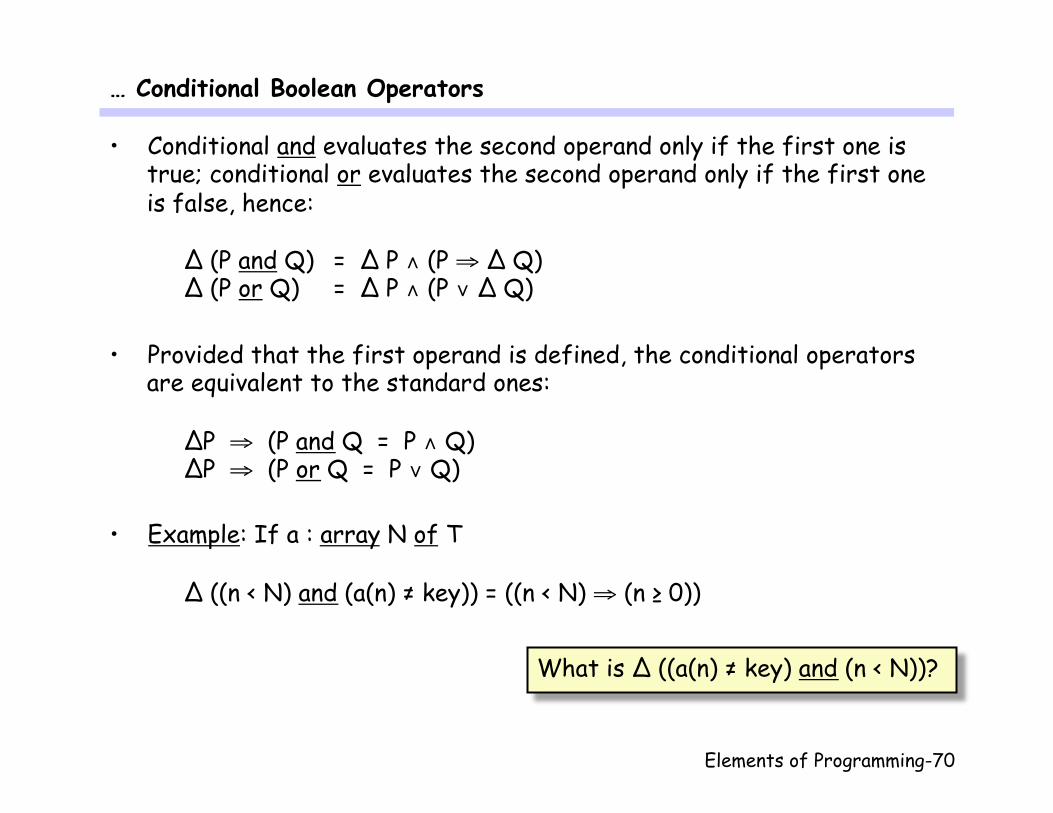
• Conditional and evaluates the second operand only if the first one is true; conditional or evaluates the second operand only if the first one is false, hence:
∆ (P and Q) = ∆ P ∧ (P ⇒ ∆ Q) ∆ (P or Q) = ∆ P ∧ (P ∨ ∆ Q)
• Provided that the first operand is defined, the conditional operators
are equivalent to the standard ones:
∆P ⇒ (P and Q = P ∧ Q) ∆P ⇒ (P or Q = P ∨ Q)
• Example: If a : array N of T
∆ ((n < N) and (a(n) ≠ key)) = ((n < N) ⇒ (n ≥ 0))
What is ∆ ((a(n) ≠ key) and (n < N))?
Elements of Programming-71
Statements with Partial Expressions
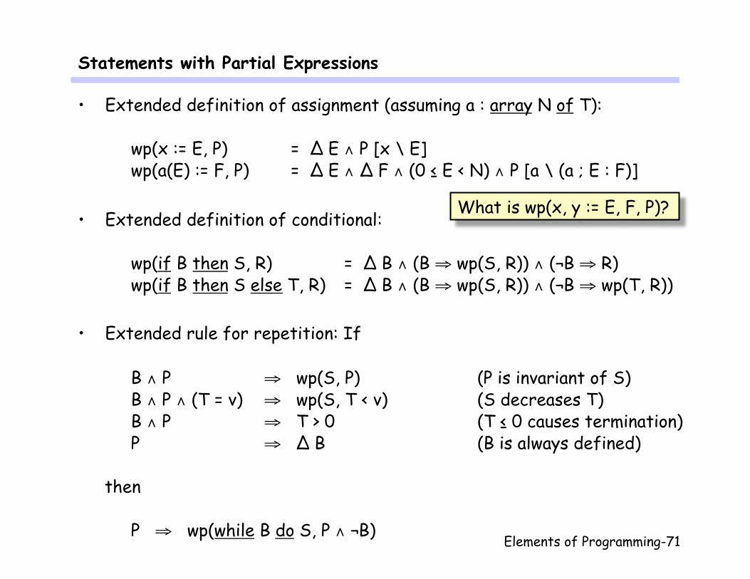
• Extended definition of assignment (assuming a : array N of T):
wp(x := E, P) = ∆ E ∧ P [x \ E] wp(a(E) := F, P) = ∆ E ∧ ∆ F ∧ (0 ≤ E < N) ∧ P [a \ (a ; E : F)]
• Extended definition of conditional:
wp(if B then S, R) = ∆ B ∧ (B ⇒ wp(S, R)) ∧ (¬B ⇒ R) wp(if B then S else T, R) = ∆ B ∧ (B ⇒ wp(S, R)) ∧ (¬B ⇒ wp(T, R))
• Extended rule for repetition: If
B ∧ P ⇒ wp(S, P) (P is invariant of S) B ∧ P ∧ (T = v) ⇒ wp(S, T < v) (S decreases T) B ∧ P ⇒ T > 0 (T ≤ 0 causes termination) P ⇒ ∆ B (B is always defined)
then
P ⇒ wp(while B do S, P ∧ ¬B)
What is wp(x, y := E, F, P)?
Elements of Programming-72
Linear Search Revisited
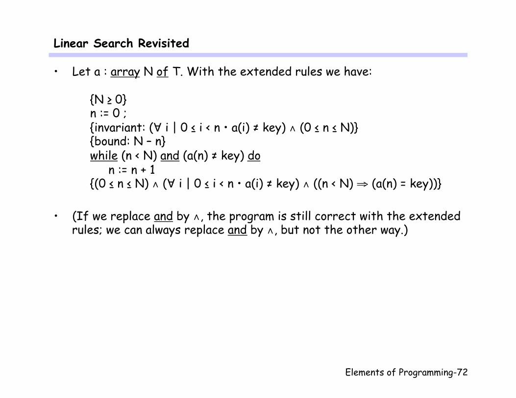
• Let a : array N of T. With the extended rules we have:
{N ≥ 0} n := 0 ; {invariant: (∀ i | 0 ≤ i < n • a(i) ≠ key) ∧ (0 ≤ n ≤ N)} {bound: N – n} while (n < N) and (a(n) ≠ key) do n := n + 1 {(0 ≤ n ≤ N) ∧ (∀ i | 0 ≤ i < n • a(i) ≠ key) ∧ ((n < N) ⇒ (a(n) = key))}
• (If we replace and by ∧, the program is still correct with the extended
rules; we can always replace and by ∧, but not the other way.)
Elements of Programming-73
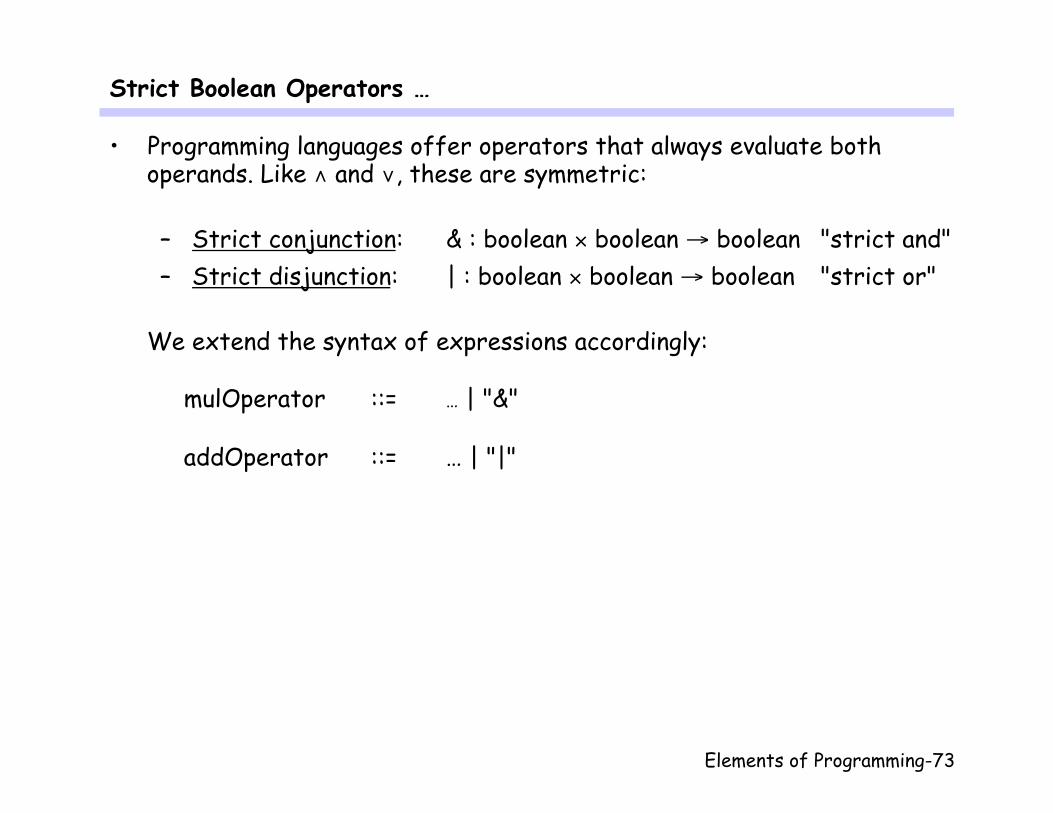
Strict Boolean Operators …
• Programming languages offer operators that always evaluate both operands. Like ∧ and ∨, these are symmetric: – Strict conjunction: & : boolean × boolean → boolean "strict and" – Strict disjunction: | : boolean × boolean → boolean "strict or"
We extend the syntax of expressions accordingly:
mulOperator ::= … | "&"
addOperator ::= … | "|"

Elements of Programming-74
… Strict Boolean Operators
• Strict boolean operators require both operands to be defined (like all arithmetic operators):
∆ (P & Q) = ∆ P ∧ ∆ Q ∆ (P | Q) = ∆ P ∧ ∆ Q
• Provided that both operands are defined, the strict operators are
equivalent to the standard ones:
∆ P ∧ ∆ Q ⇒ (P & Q = P ∧ Q) ∆ P ∧ ∆ Q ⇒ (P | Q = P ∨ Q)
• Example: If we write the loop of the linear search as
while (n < N) & (a(n) ≠ key) do n := n + 1
the program is not correct w.r.t. the given pre- and postcondition.
What is ∆ ((n < N) & (a(n) ≠ key))?
Elements of Programming-75
Boolean Operator in Programming Languages
• Historically, Pascal defines and and or strict (as & and |) so that compilers could use the symmetry for optimizations. Nowadays, most compilers implement and and or conditionally.
• Java and C define & and | strict and && and || conditionally (as and and or).
• Eiffel and Ada define and and or strict (as & and |) and and then and or else conditionally (as and and or).
• Modula-2 defines AND and OR conditionally (as and and or).
• No language implements mathematical ∧ and ∨. Strictly speaking their use is not allowed in concrete programs even though we will continue to do so, with the understanding that they can be appropriately replaced by and and or.
Elements of Programming-76
Coping with Machine Limitations
• Previous definition of ∆ assumed unbounded arithmetic. As integers are typically limited to the word size of the machine or a small multiple thereof, we consider instead:
∆ (E + F) = ∆ E ∧ ∆ F ∧ (MININT ≤ E + F ≤ MAXINT) ∆ (E – F) = ∆ E ∧ ∆ F ∧ (MININT ≤ E – F ≤ MAXINT) ∆ (E · F) = ∆ E ∧ ∆ F ∧ (MININT ≤ E · F ≤ MAXINT)
where MININT and MAXINT are the smallest and largest representable integer, respectively.
• However, while division by zero is clearly a "design error", an arithmetic overflow or underflow is an "implementation error" – a limitation of the underlying machine which has not been taken into account in the design.
• When analyzing programs, we have to be careful whether we consider the possibility of arithmetic overflow or not!
Elements of Programming-77
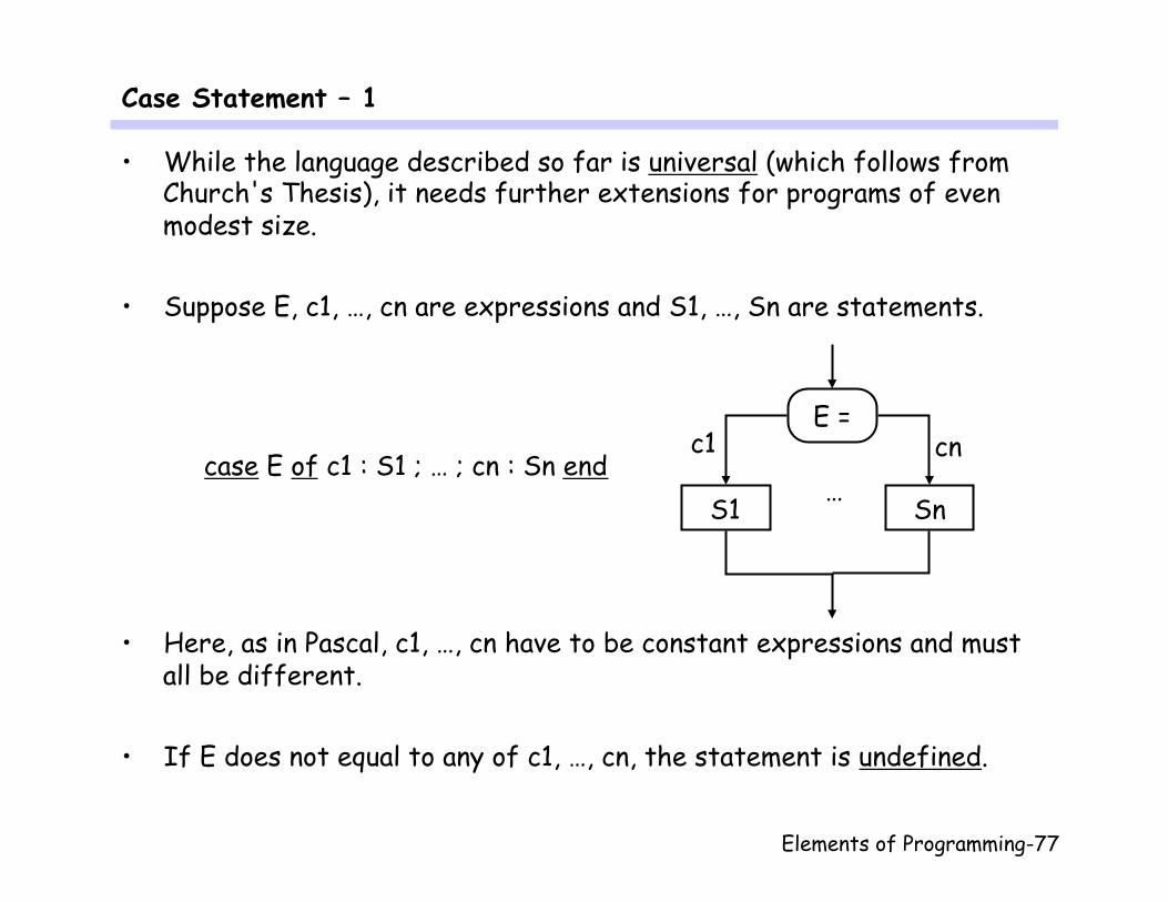
Case Statement – 1
• While the language described so far is universal (which follows from Church's Thesis), it needs further extensions for programs of even modest size.
• Suppose E, c1, …, cn are expressions and S1, …, Sn are statements.
case E of c1 : S1 ; … ; cn : Sn end
• Here, as in Pascal, c1, …, cn have to be constant expressions and must
all be different.
• If E does not equal to any of c1, …, cn, the statement is undefined.
E =
S1 Sn …
c1 cn

Elements of Programming-78
Case Statement – 2
• A case may have several labels:
c, d : S stands for c : S ; d : S
• We extend the syntax of statements accordingly:
statement ::= … | case expression of caseList end
caseList ::= expressionList : statementSequence | caseList ; expressionList : statementSequence
Elements of Programming-79
Case Statement – 3
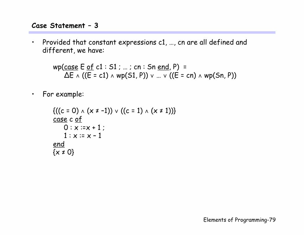
• Provided that constant expressions c1, …, cn are all defined and different, we have:
wp(case E of c1 : S1 ; … ; cn : Sn end, P) = ∆E ∧ ((E = c1) ∧ wp(S1, P)) ∨ … ∨ ((E = cn) ∧ wp(Sn, P))
• For example:
{((c = 0) ∧ (x ≠ –1)) ∨ ((c = 1) ∧ (x ≠ 1))} case c of 0 : x :=x + 1 ; 1 : x := x – 1 end {x ≠ 0}
Elements of Programming-80
Repeat Statement …
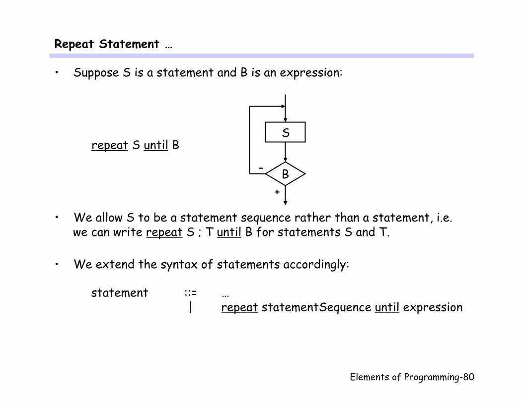
• Suppose S is a statement and B is an expression:
repeat S until B
• We allow S to be a statement sequence rather than a statement, i.e. we can write repeat S ; T until B for statements S and T.
• We extend the syntax of statements accordingly:
statement ::= … | repeat statementSequence until expression
+
–
S
B

Elements of Programming-81
… Repeat Statement
• Following rule is derived by defining: repeat S until B = S ; while ¬B do S
Let – P, Q be a predicates, where Q is the invariant; – T be an integer expression, the bound; – v be an auxiliary integer variable.
If
P ⇒ wp(S, Q) (S establishes Q) ¬B ∧ Q ⇒ wp(S, Q) (Q is invariant of S) ¬B ∧ Q ∧ (T = v) ⇒ wp(S, T < v) (S decreases T) ¬B ∧ Q ⇒ T > 0 (T ≤ 0 causes termination)
Q ⇒ ∆ B (B is always defined) then
P ⇒ wp(repeat S until B, Q ∧ B)
Elements of Programming-82
Sum of Array Elements Revisited
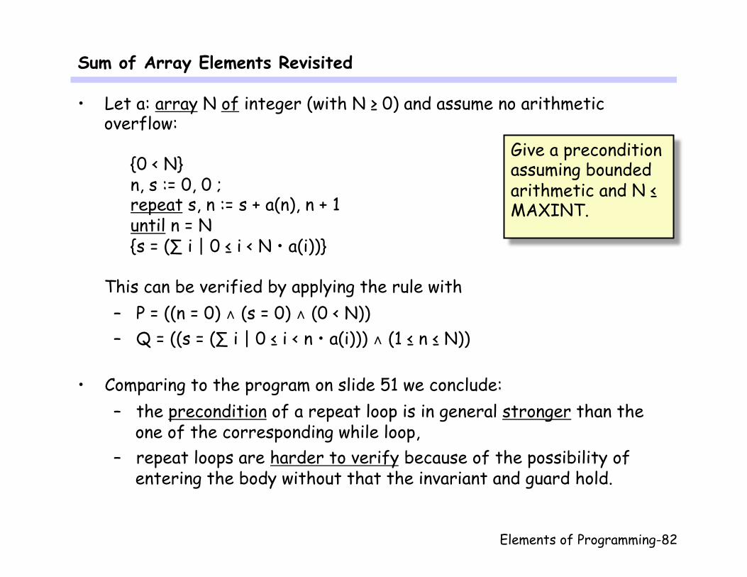
• Let a: array N of integer (with N ≥ 0) and assume no arithmetic overflow:
{0 < N} n, s := 0, 0 ; repeat s, n := s + a(n), n + 1 until n = N {s = (∑ i | 0 ≤ i < N • a(i))}
This can be verified by applying the rule with – P = ((n = 0) ∧ (s = 0) ∧ (0 < N)) – Q = ((s = (∑ i | 0 ≤ i < n • a(i))) ∧ (1 ≤ n ≤ N))
• Comparing to the program on slide 51 we conclude:
– the precondition of a repeat loop is in general stronger than the one of the corresponding while loop,
– repeat loops are harder to verify because of the possibility of entering the body without that the invariant and guard hold.
Give a precondition assuming bounded arithmetic and N ≤ MAXINT.

Elements of Programming-83
Variable Declarations – 1
• A variable declaration introduces a local (bound) variable with a scope, like a quantification. Let x be an identifier, T a type, S a statement:
var x : T ; S
• Several variables may be declared at once and several variables may be declared to have the same type:
var x1 : T1, …, xn : Tn stands for var x1 : T1 ; … ; var xn : Tn x1, …, xn : T stands for x1 : T, …, xn : T
• We extend the syntax of statements accordingly:
statement ::= …
| declaration ; statement declaration ::= var variableList
Elements of Programming-84
Variable Declarations – 2
• We continue with the syntax: variableList ::= identifierList : type
| variableList , identifierList : type
• Note that we allow variable declarations to appear anywhere in programs, like in C but unlike in Pascal, where variable declarations can be only at the outermost level.
• The body has to be prepared for an arbitrary initial value of the declared variable. Let x be a variable that does not occur in P:
wp(var x : T ; S, P) = (∀ x : T • wp(S, P))
Elements of Programming-85
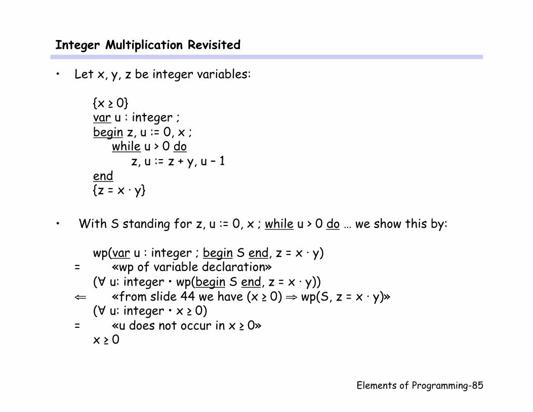
Integer Multiplication Revisited
• Let x, y, z be integer variables:
{x ≥ 0} var u : integer ; begin z, u := 0, x ; while u > 0 do z, u := z + y, u – 1 end {z = x · y}
• With S standing for z, u := 0, x ; while u > 0 do … we show this by:
wp(var u : integer ; begin S end, z = x · y)
= «wp of variable declaration» (∀ u: integer • wp(begin S end, z = x · y))
⇐ «from slide 44 we have (x ≥ 0) ⇒ wp(S, z = x · y)» (∀ u: integer • x ≥ 0)
= «u does not occur in x ≥ 0» x ≥ 0

Elements of Programming-86
Stepwise Refinement
• No serious program can be conceived in one step. We therefore develop programs by a series of refinement steps. For example, in one step, we – select a specific algorithm or a data structure, – make some transformations (for efficiency), – elaborate on what to do in exceptional situations (for robustness), – generalize parts of the program (for reusability).
• The phrase "Program Development by Stepwise Refinement" was
coined by N. Wirth and applied in a hierarchical fashion: Note that in practice programs are rarely developed this way. Still, this is a good way of explaining the program and documenting the development.
begin … ; … ; end
while … do …
if … then … else …

Elements of Programming-87
Printing Images – 1
• Let a printer be given that is controlled by following commands: – newLine: start a new line at the leftmost position – advance: move the print head one position to the right – print: print a dot and move one position to the right
Our task is to print an image given by the functions fx, fy, where
∀ i | 0 ≤ i < N • (0 ≤ fx(i) < X) ∧ (0 ≤ fy(i) < Y) More specifically, fx and fy could be arrays rather than functions. We take, for example, N = 1000, X = 100, Y = 50.
• Our idea is to compute and store the image first and then to output it on the device line by line. – This assumes we can afford storing the whole image. – It does not require that the values fx(i), fy(i) need to be computed
several times.
Suggest an alternative approach!
Elements of Programming-88
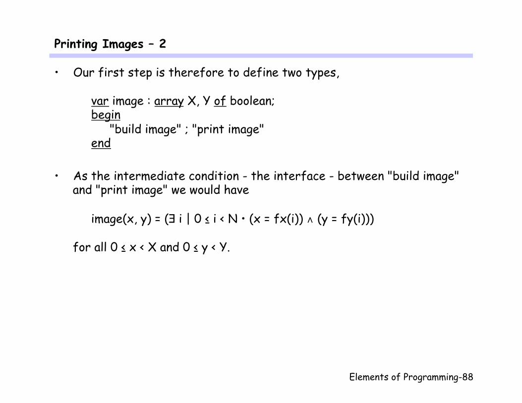
Printing Images – 2
• Our first step is therefore to define two types,
var image : array X, Y of boolean; begin "build image" ; "print image" end
• As the intermediate condition - the interface - between "build image"
and "print image" we would have
image(x, y) = (∃ i | 0 ≤ i < N • (x = fx(i)) ∧ (y = fy(i))) for all 0 ≤ x < X and 0 ≤ y < Y.
Elements of Programming-89
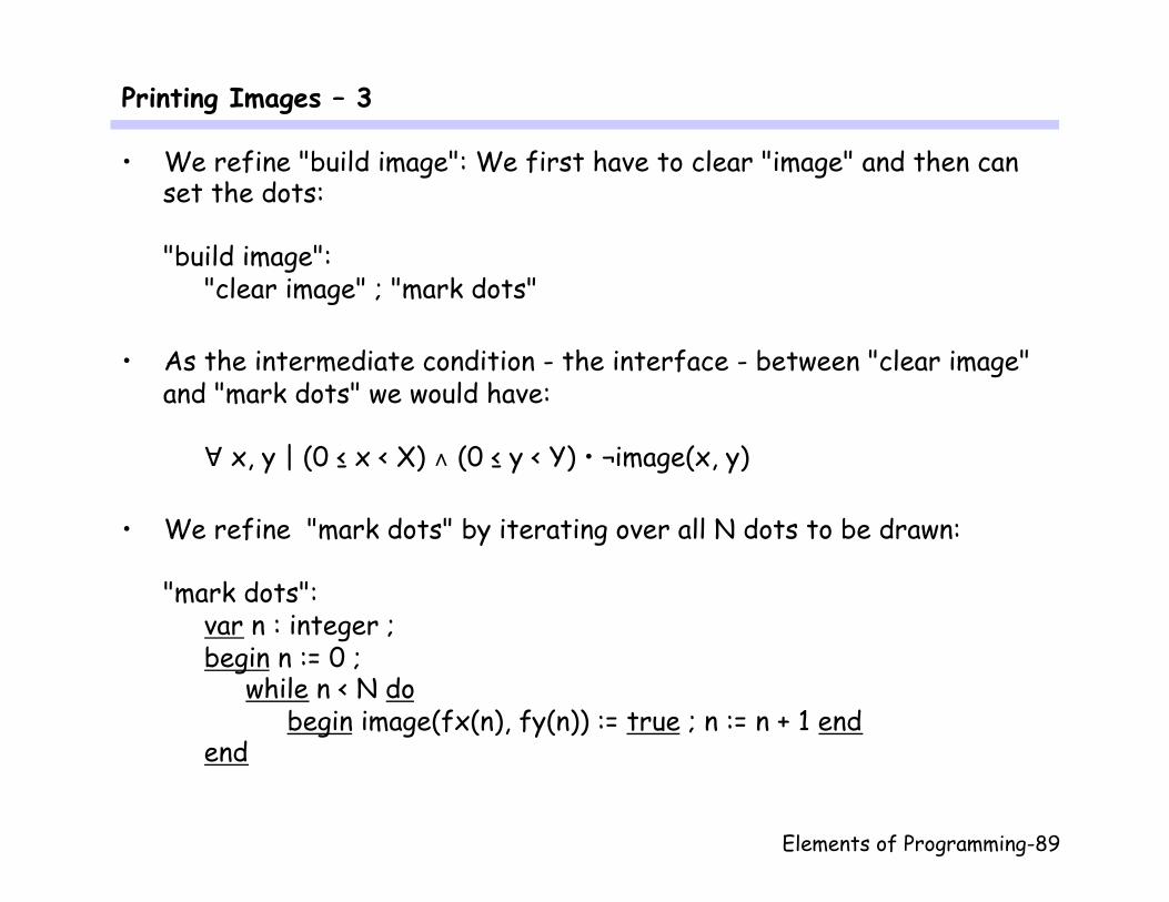
Printing Images – 3
• We refine "build image": We first have to clear "image" and then can set the dots: "build image":
"clear image" ; "mark dots"
• As the intermediate condition - the interface - between "clear image" and "mark dots" we would have:
∀ x, y | (0 ≤ x < X) ∧ (0 ≤ y < Y) • ¬image(x, y)
• We refine "mark dots" by iterating over all N dots to be drawn: "mark dots":
var n : integer ; begin n := 0 ; while n < N do begin image(fx(n), fy(n)) := true ; n := n + 1 end end
Elements of Programming-90
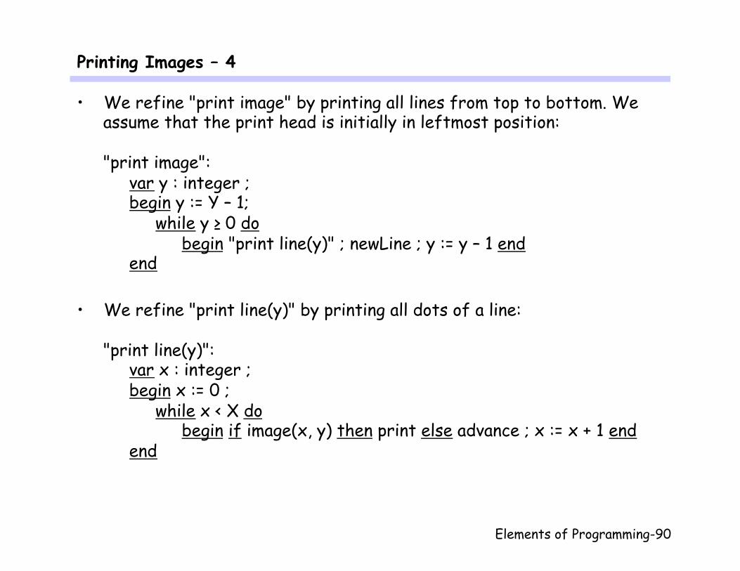
Printing Images – 4
• We refine "print image" by printing all lines from top to bottom. We assume that the print head is initially in leftmost position: "print image":
var y : integer ; begin y := Y – 1; while y ≥ 0 do begin "print line(y)" ; newLine ; y := y – 1 end end
• We refine "print line(y)" by printing all dots of a line:
"print line(y)":
var x : integer ; begin x := 0 ; while x < X do begin if image(x, y) then print else advance ; x := x + 1 end end

Elements of Programming-91
Printing Images – 5
• We refine "clear image" by clearing all lines: "clear image":
var y : integer ; begin y := Y – 1 ; while y ≥ 0 do begin "clear line(y)" ; y := y – 1 end end
• Finally we refine "clear line(y)" by clearing all dots of line y:
"clear line(y)":
var x : integer ; begin x := 0 ; while x < X do begin image(x, y) := false ; x := x + 1 end end

Elements of Programming-92
Procedure Declarations …
• Procedures introduce three aspects: – naming – parameter passing – recursion
(Pascal additionally connects local variables to procedures.)
• We extend the syntax of statements and declarations accordingly: statement ::= …
| identifier ( expressionList , identifierList ) declaration ::= ...
| procedure identifier ( variableList , var variableList ) statement
Note: a procedure declaration may be with value or without result parameters or without both and likewise for the call. We omit the corresponding cases in the grammar for brevity.

Elements of Programming-93
… Procedure Declarations
• The call of a procedure can always be replaced by its body, known as the copy rule. If p is declared by
procedure p(v : V, var r : R) S and e : V is an expression and x : R is a variable, we define:
p(e, x) = var v : V, r : R ; begin v := e ; S ; x := r end
• For example, if increment is declared by
procedure increment(d : integer) c := c + d then
increment(3) = «copy rule»
var d : integer ; begin d := 3 ; c := c + d end = «simplifications»
c := c + 3

Elements of Programming-94
Function Procedures and return statements
• A function procedure is a procedure with a single result parameter. We allow an alternative syntax for declaration and call:
procedure p(v : V) : R x := p(e) S
are equivalent to
procedure p(v : V, var result : R) p(e, x) S
• A return statement assigns to the result parameter:
return e
is equivalent to
result := e

Elements of Programming-95
Rule for Procedure Calls…
• Suppose procedure p is declared by
procedure p(v : V, var r : R) S and we have:
{P} S {Q} Then
{P [v \ e]} p(e, x) {Q [v, r \ e, x]} provided that: – x does not occur in Q and e – r does not occur in P and e – S does not assign to v and variables of e
Elements of Programming-96
… Rule for Procedure Calls
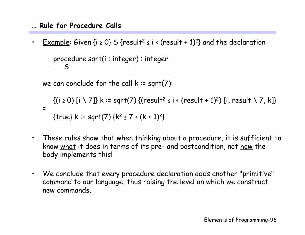
• Example: Given {i ≥ 0} S {result2 ≤ i < (result + 1)2} and the declaration
procedure sqrt(i : integer) : integer S
we can conclude for the call k := sqrt(7):
{(i ≥ 0) [i \ 7]} k := sqrt(7) {(result2 ≤ i < (result + 1)2) [i, result \ 7, k]} =
{true} k := sqrt(7) {k2 ≤ 7 < (k + 1)2}
• These rules show that when thinking about a procedure, it is sufficient to know what it does in terms of its pre- and postcondition, not how the body implements this!
• We conclude that every procedure declaration adds another "primitive" command to our language, thus raising the level on which we construct new commands.
Elements of Programming-97
Printing Images Revisited
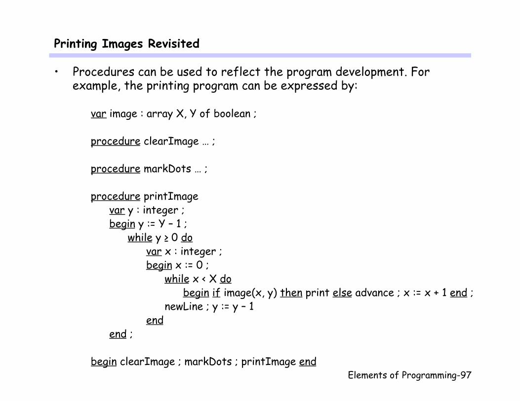
• Procedures can be used to reflect the program development. For example, the printing program can be expressed by:
var image : array X, Y of boolean ;
procedure clearImage … ;
procedure markDots … ;
procedure printImage var y : integer ; begin y := Y – 1 ; while y ≥ 0 do var x : integer ; begin x := 0 ; while x < X do begin if image(x, y) then print else advance ; x := x + 1 end ; newLine ; y := y – 1 end end ;
begin clearImage ; markDots ; printImage end
Elements of Programming-98
Programming Style – 1
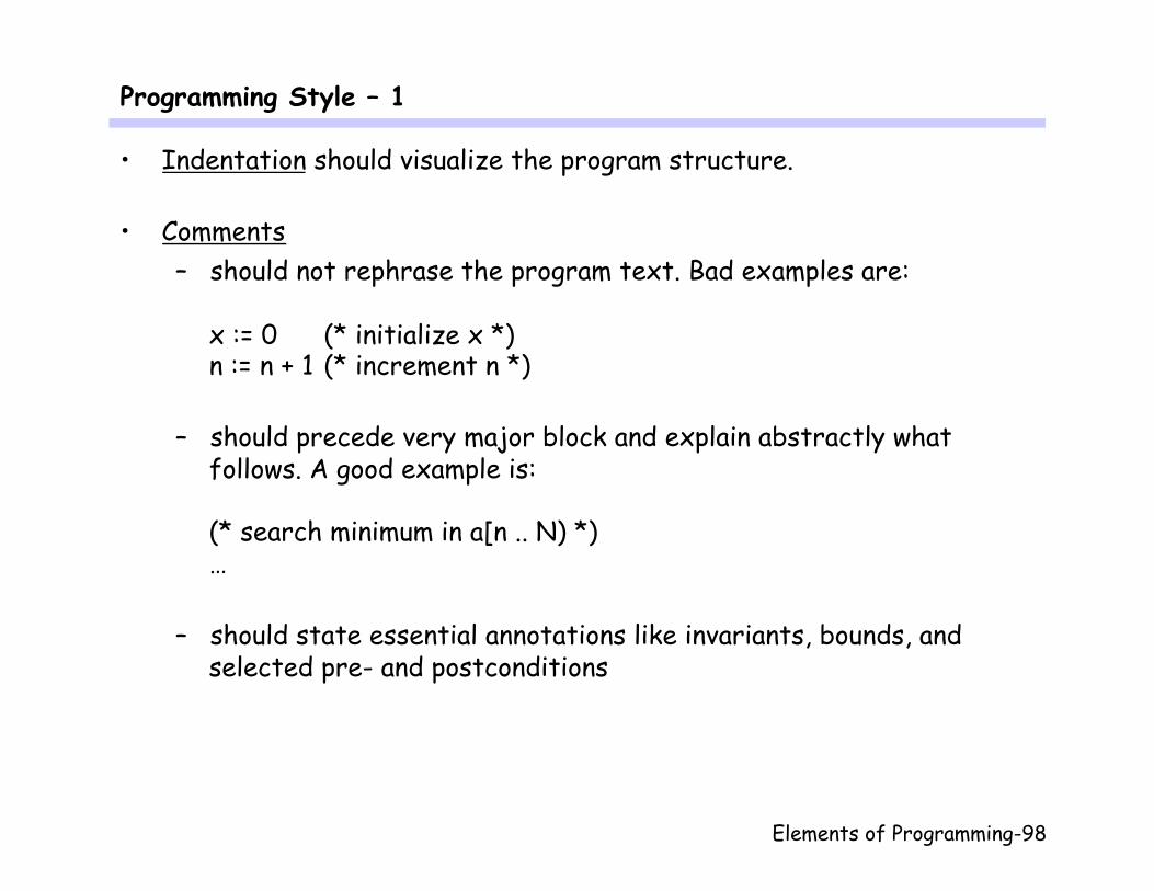
• Indentation should visualize the program structure.
• Comments – should not rephrase the program text. Bad examples are:
x := 0 (* initialize x *) n := n + 1 (* increment n *)
– should precede very major block and explain abstractly what follows. A good example is: (* search minimum in a[n .. N) *) …
– should state essential annotations like invariants, bounds, and selected pre- and postconditions

Elements of Programming-99
Programming Style – 2
• Names – should be readable. Bad names are:
avrg, hdr, fopen, _x_2
– should have consistent capitalization, for example N, MAXINT constants in capitals List, Node types starting with capital displayDialog, sort operations starting with lower case employees, average variables starting with lower case
– should be grammatically sensible, that is: • noun phrases for constants, types, variables • verb phrases for operations • adjectives for boolean variables and boolean operations, for
example queueEmpty, isClosed.
Elements of Programming-100
Programming Style – 3
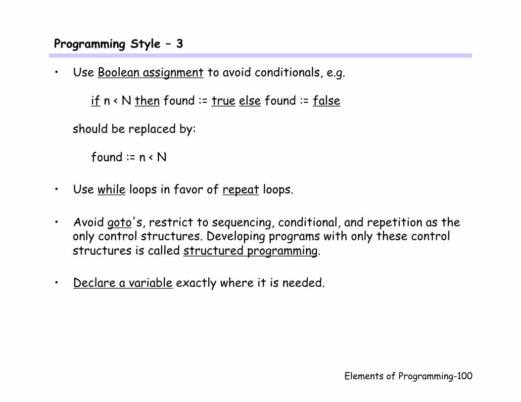
• Use Boolean assignment to avoid conditionals, e.g.
if n < N then found := true else found := false should be replaced by:
found := n < N
• Use while loops in favor of repeat loops.
• Avoid goto's, restrict to sequencing, conditional, and repetition as the only control structures. Developing programs with only these control structures is called structured programming.
• Declare a variable exactly where it is needed.

Elements of Programming-101
Hints for Implementation in Pascal and C
• In C booleans have to be mapped to integers. In Pascal and C implication a ⇒ b is written as a <= b.
• Value parameters and function results are present in Pascal and C, result parameters are mapped to reference parameters, e.g.:
procedure has(x : integer, var h : boolean) (*result parameter h*) is mapped to:
procedure has(x: integer; var h: boolean); (*reference parameter h*)
• Reference parameters may lead to aliasing, e.g. in Pascal procedure n(var v, w : integer) begin v := 3; w := 4 end
establishes postcondition v < w but the call n(x, x)
does not establish x < x!

Elements of Programming-102
For Statement …
• The for loop specifies an iteration over elements in a given range, and therefor corresponds to the structure of arrays. We consider: for x := E to F do S = var x : integer ;
begin x := E ; while x ≤ F do begin S ; x := x + 1 end end
for x := E downto F do S = var x : integer ;
begin x := E ; while x ≥ F do begin S ; x := x – 1 end end
• Note that C and Java allow the variable to be made local, Pascal does
not. However, Pascal does not guarantee any specific final value of x. Some Pascal compilers forbid assignments to x in S, C and Java don't.

Elements of Programming-103
… For Statement
• We extend the syntax of statements accordingly:
statement ::= … | for identifier := expression to expression do statement | for identifier := expression downto expression do statement
• If the variable is not assigned in the statement, the for loop guarantees
termination. Let P be a predicate, the invariant. If x does not occur in E, F and E, F, x are not changed by S and (E ≤ x ≤ F) ∧ P ⇒ wp(S, P [x \ x + 1]) (P is invariant of S)
then
∆E ∧ ∆F ∧ (E ≤ F + 1) ∧ P [x \ E] ⇒ wp(for x := E to F do S, P [x \ F + 1])
Elements of Programming-104
Printing Images Revisited
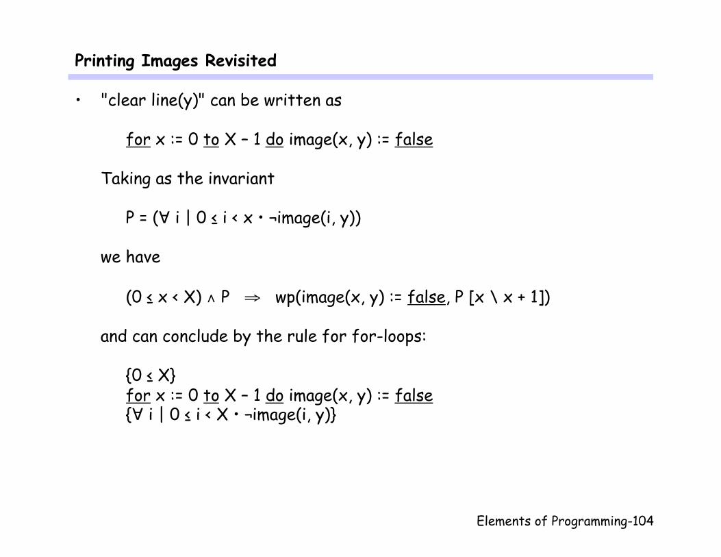
• "clear line(y)" can be written as
for x := 0 to X – 1 do image(x, y) := false Taking as the invariant
P = (∀ i | 0 ≤ i < x • ¬image(i, y)) we have
(0 ≤ x < X) ∧ P ⇒ wp(image(x, y) := false, P [x \ x + 1]) and can conclude by the rule for for-loops:
{0 ≤ X} for x := 0 to X – 1 do image(x, y) := false {∀ i | 0 ≤ i < X • ¬image(i, y)}
Elements of Programming-105
Repeat Statement Revisited
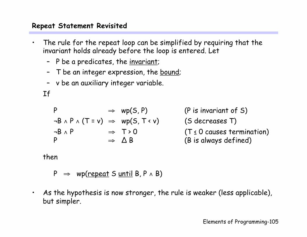
• The rule for the repeat loop can be simplified by requiring that the invariant holds already before the loop is entered. Let – P be a predicates, the invariant; – T be an integer expression, the bound; – v be an auxiliary integer variable.
If
P ⇒ wp(S, P) (P is invariant of S) ¬B ∧ P ∧ (T = v) ⇒ wp(S, T < v) (S decreases T) ¬B ∧ P ⇒ T > 0 (T ≤ 0 causes termination)
P ⇒ ∆ B (B is always defined) then
P ⇒ wp(repeat S until B, P ∧ B)
• As the hypothesis is now stronger, the rule is weaker (less applicable), but simpler.
Elements of Programming-106
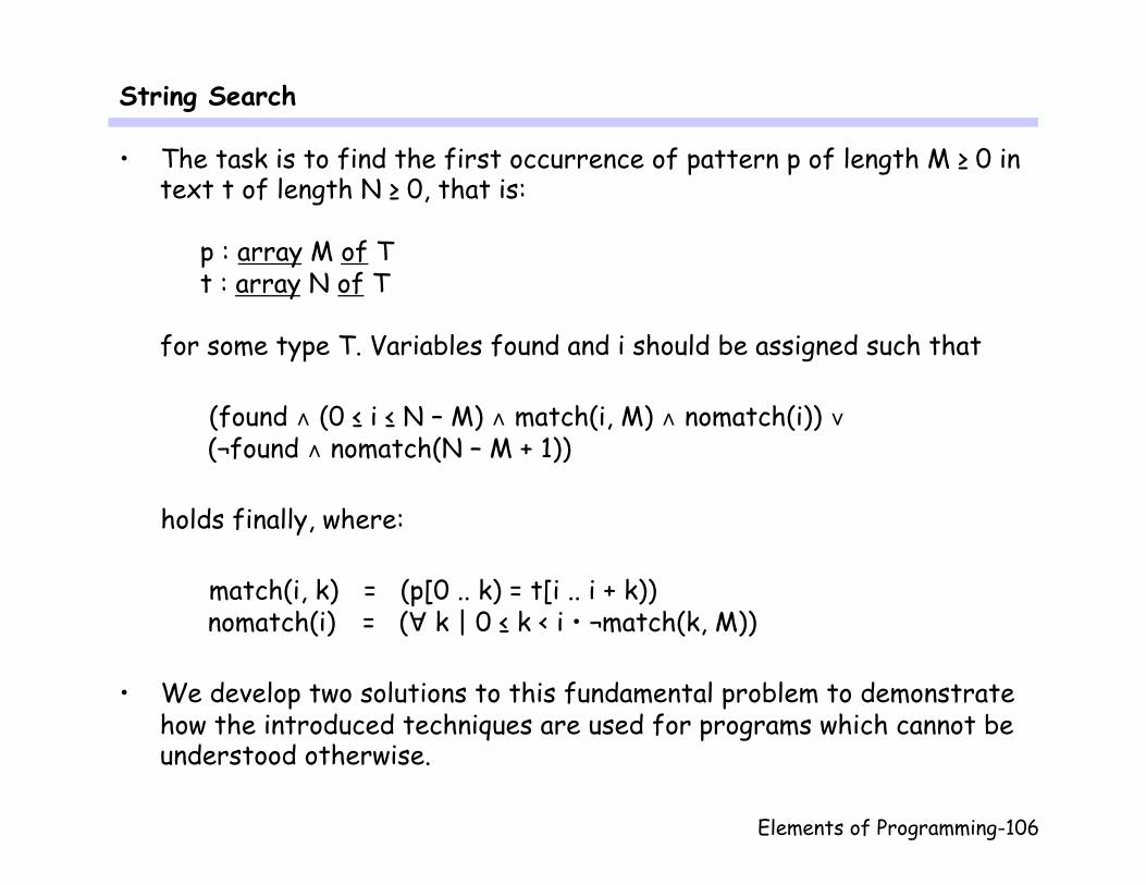
String Search
• The task is to find the first occurrence of pattern p of length M ≥ 0 in text t of length N ≥ 0, that is:
p : array M of T t : array N of T
for some type T. Variables found and i should be assigned such that
(found ∧ (0 ≤ i ≤ N – M) ∧ match(i, M) ∧ nomatch(i)) ∨ (¬found ∧ nomatch(N – M + 1))
holds finally, where:
match(i, k) = (p[0 .. k) = t[i .. i + k)) nomatch(i) = (∀ k | 0 ≤ k < i • ¬match(k, M))
• We develop two solutions to this fundamental problem to demonstrate how the introduced techniques are used for programs which cannot be understood otherwise.

Elements of Programming-107
Naive String Search – 1
• A straightforward solution is to start comparing p with t at the left end of t and in case of a mismatch shift the position of p:
{N ≥ M} i := –1 ; {invariant: nomatch(i + 1) ∧ (–1 ≤ i ≤ N – M)} repeat i := i + 1 ; {nomatch(i)}
"compare p with t at position i" until "p matches t" ∨ (i = N – M) ; found := "p matches t"
• For the invariant, we observe that – nomatch(0) holds initially, – "p matches t" means match(i, M), – nomatch(i) and ¬match(i, M) implies nomatch(i + 1), hence the
invariant is preserved.
t0 t1 … ti ti+1 … ti+M–1 … tN-1
p0 p1 … pM-1 shift
Elements of Programming-108
Naive String Search – 2
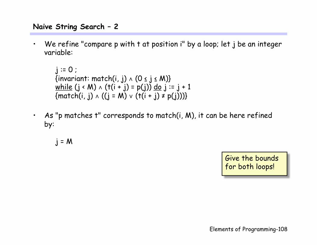
• We refine "compare p with t at position i" by a loop; let j be an integer variable:
j := 0 ; {invariant: match(i, j) ∧ (0 ≤ j ≤ M)} while (j < M) ∧ (t(i + j) = p(j)) do j := j + 1 {match(i, j) ∧ ((j = M) ∨ (t(i + j) ≠ p(j)))}
• As "p matches t" corresponds to match(i, M), it can be here refined
by:
j = M
Give the bounds for both loops!
Elements of Programming-109
Naive String Search – 3
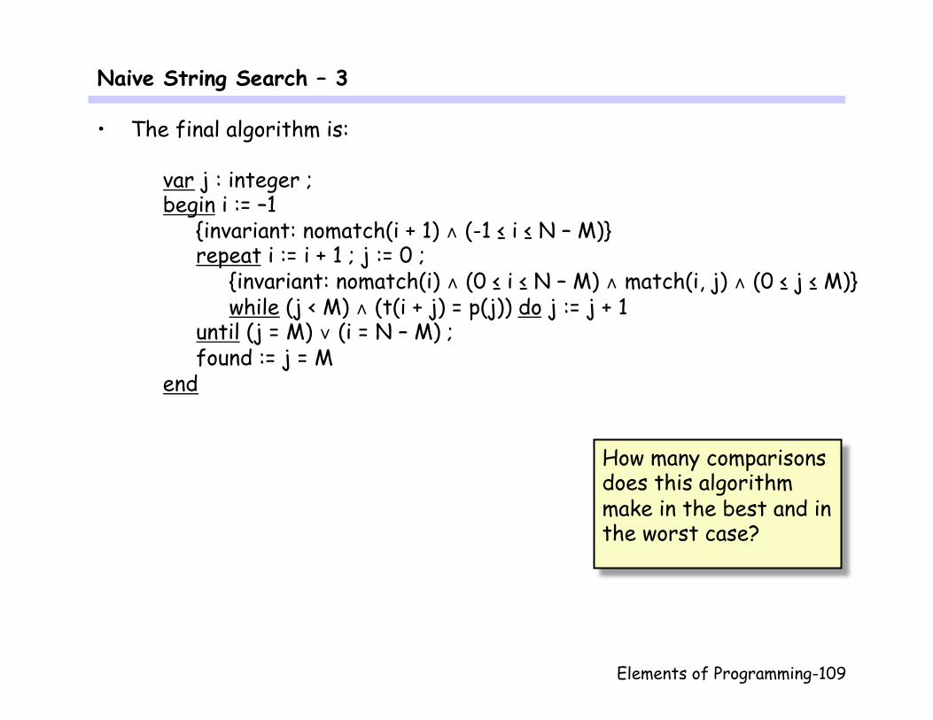
• The final algorithm is:
var j : integer ; begin i := –1 {invariant: nomatch(i + 1) ∧ (-1 ≤ i ≤ N – M)} repeat i := i + 1 ; j := 0 ; {invariant: nomatch(i) ∧ (0 ≤ i ≤ N – M) ∧ match(i, j) ∧ (0 ≤ j ≤ M)} while (j < M) ∧ (t(i + j) = p(j)) do j := j + 1 until (j = M) ∨ (i = N – M) ; found := j = M end
How many comparisons does this algorithm make in the best and in the worst case?
Elements of Programming-110
Boyer-Moore Search – 1
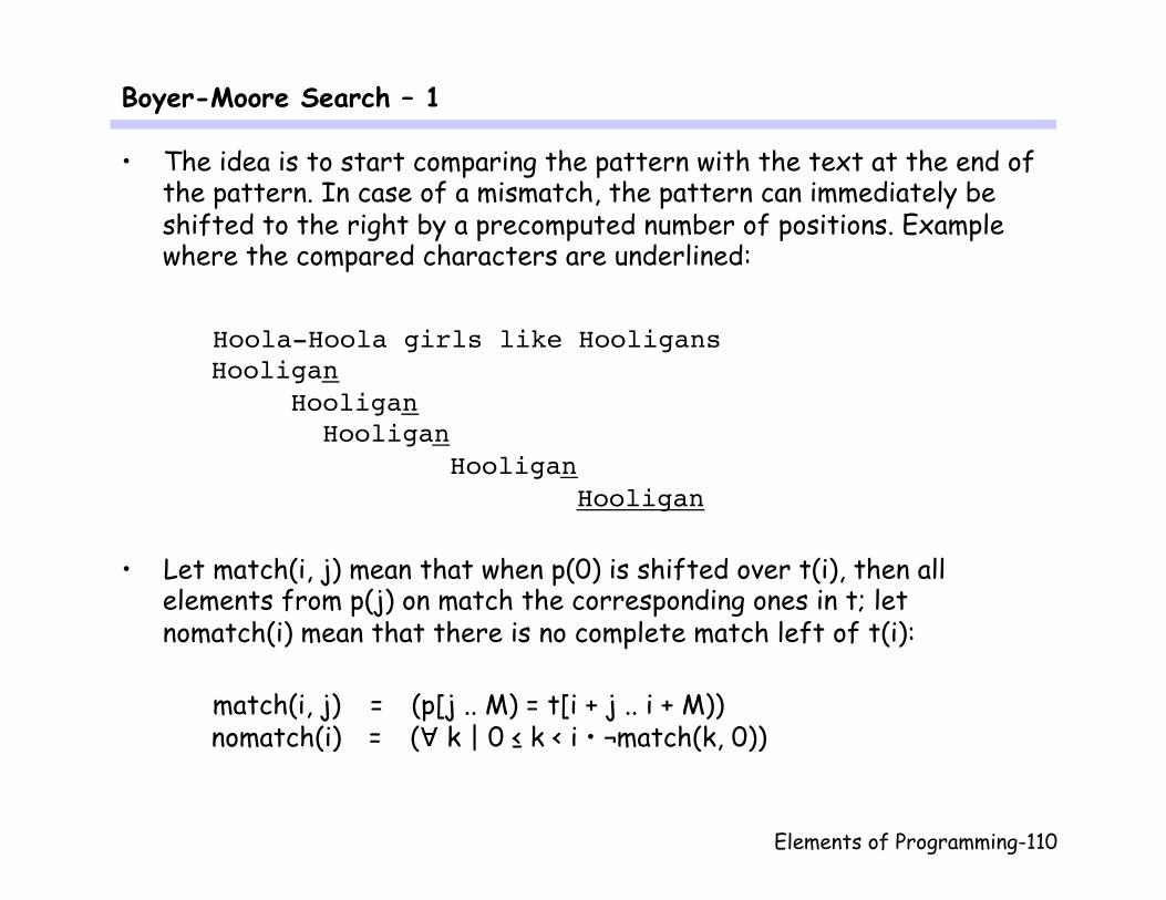
• The idea is to start comparing the pattern with the text at the end of the pattern. In case of a mismatch, the pattern can immediately be shifted to the right by a precomputed number of positions. Example where the compared characters are underlined:
Hoola-Hoola girls like Hooligans Hooligan Hooligan Hooligan Hooligan Hooligan
• Let match(i, j) mean that when p(0) is shifted over t(i), then all elements from p(j) on match the corresponding ones in t; let nomatch(i) mean that there is no complete match left of t(i):
match(i, j) = (p[j .. M) = t[i + j .. i + M)) nomatch(i) = (∀ k | 0 ≤ k < i • ¬match(k, 0))
Elements of Programming-111
Boyer-Moore Search – 2
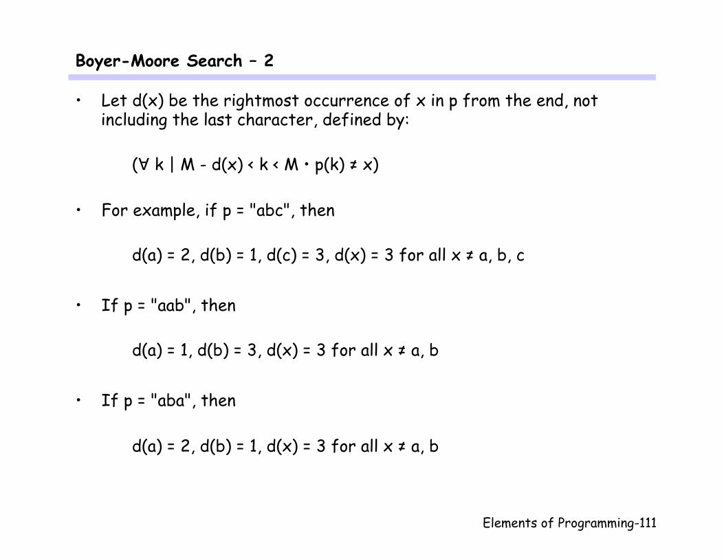
• Let d(x) be the rightmost occurrence of x in p from the end, not including the last character, defined by:
(∀ k | M - d(x) < k < M • p(k) ≠ x)
• For example, if p = "abc", then
d(a) = 2, d(b) = 1, d(c) = 3, d(x) = 3 for all x ≠ a, b, c • If p = "aab", then
d(a) = 1, d(b) = 3, d(x) = 3 for all x ≠ a, b
• If p = "aba", then
d(a) = 2, d(b) = 1, d(x) = 3 for all x ≠ a, b
Elements of Programming-112
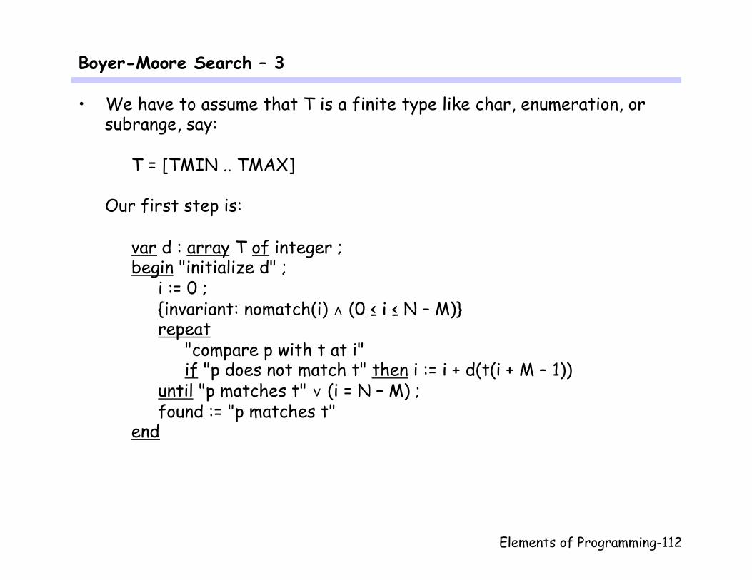
Boyer-Moore Search – 3
• We have to assume that T is a finite type like char, enumeration, or subrange, say:
T = [TMIN .. TMAX] Our first step is:
var d : array T of integer ; begin "initialize d" ; i := 0 ; {invariant: nomatch(i) ∧ (0 ≤ i ≤ N – M)} repeat "compare p with t at i" if "p does not match t" then i := i + d(t(i + M – 1)) until "p matches t" ∨ (i = N – M) ; found := "p matches t" end
Elements of Programming-113
Boyer-Moore Search – 4
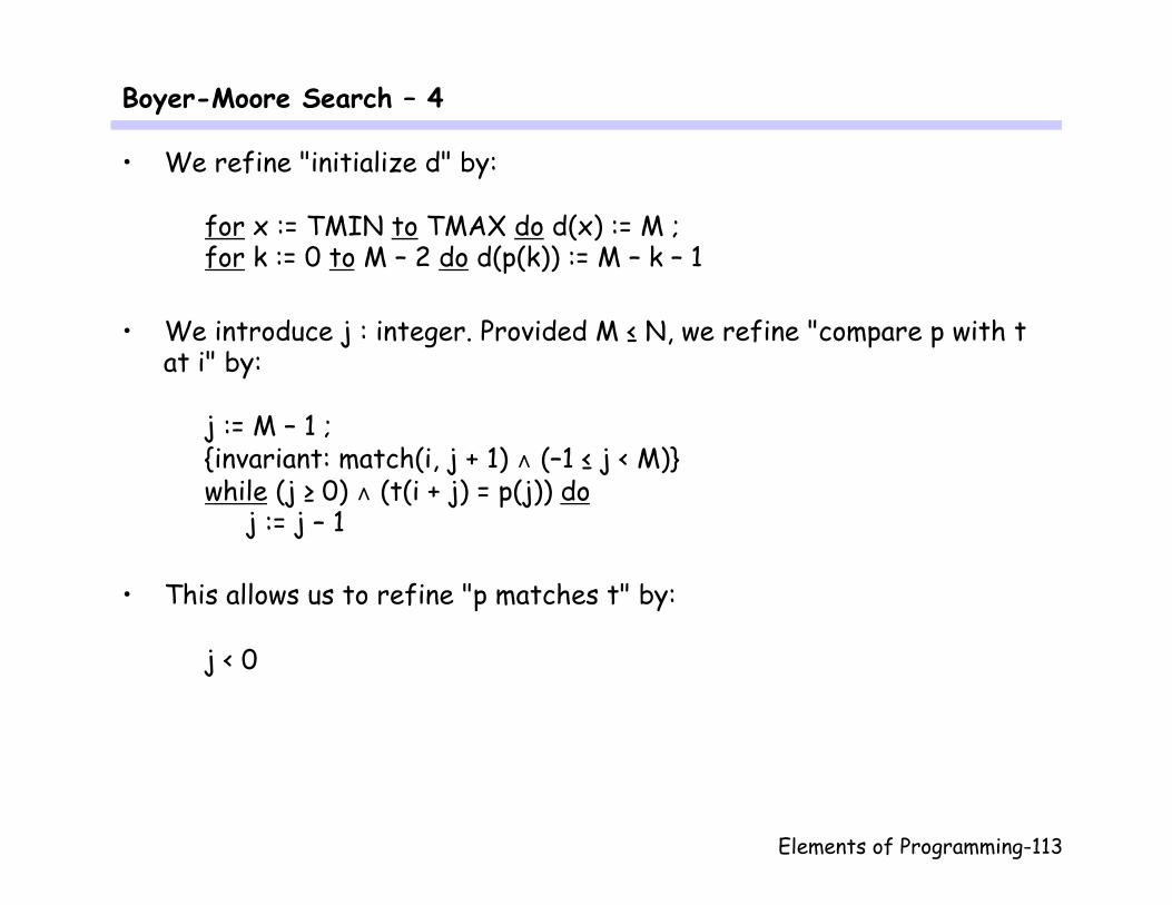
• We refine "initialize d" by:
for x := TMIN to TMAX do d(x) := M ; for k := 0 to M – 2 do d(p(k)) := M – k – 1
• We introduce j : integer. Provided M ≤ N, we refine "compare p with t
at i" by:
j := M – 1 ; {invariant: match(i, j + 1) ∧ (–1 ≤ j < M)} while (j ≥ 0) ∧ (t(i + j) = p(j)) do j := j – 1
• This allows us to refine "p matches t" by:
j < 0
Elements of Programming-114
Boyer-Moore Search – 5
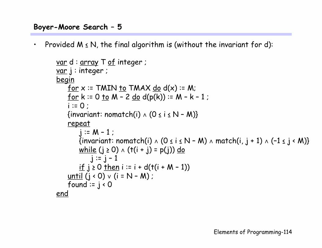
• Provided M ≤ N, the final algorithm is (without the invariant for d):
var d : array T of integer ; var j : integer ; begin for x := TMIN to TMAX do d(x) := M; for k := 0 to M – 2 do d(p(k)) := M – k – 1 ; i := 0 ; {invariant: nomatch(i) ∧ (0 ≤ i ≤ N – M)} repeat j := M – 1 ; {invariant: nomatch(i) ∧ (0 ≤ i ≤ N – M) ∧ match(i, j + 1) ∧ (–1 ≤ j < M)} while (j ≥ 0) ∧ (t(i + j) = p(j)) do j := j – 1 if j ≥ 0 then i := i + d(t(i + M – 1)) until (j < 0) ∨ (i = N – M) ; found := j < 0 end
Elements of Programming-115
Recursive Procedures
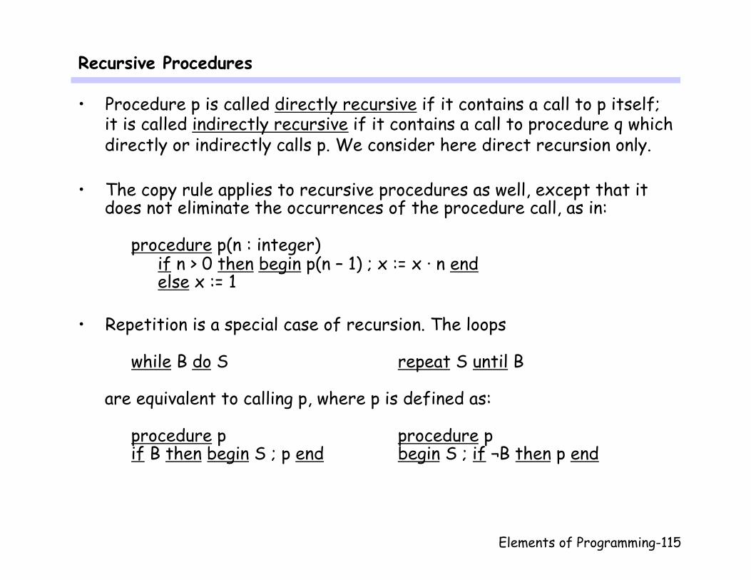
• Procedure p is called directly recursive if it contains a call to p itself; it is called indirectly recursive if it contains a call to procedure q which directly or indirectly calls p. We consider here direct recursion only.
• The copy rule applies to recursive procedures as well, except that it does not eliminate the occurrences of the procedure call, as in:
procedure p(n : integer) if n > 0 then begin p(n – 1) ; x := x · n end else x := 1
• Repetition is a special case of recursion. The loops
while B do S repeat S until B
are equivalent to calling p, where p is defined as:
procedure p procedure p if B then begin S ; p end begin S ; if ¬B then p end
Elements of Programming-116
Tail Recursion
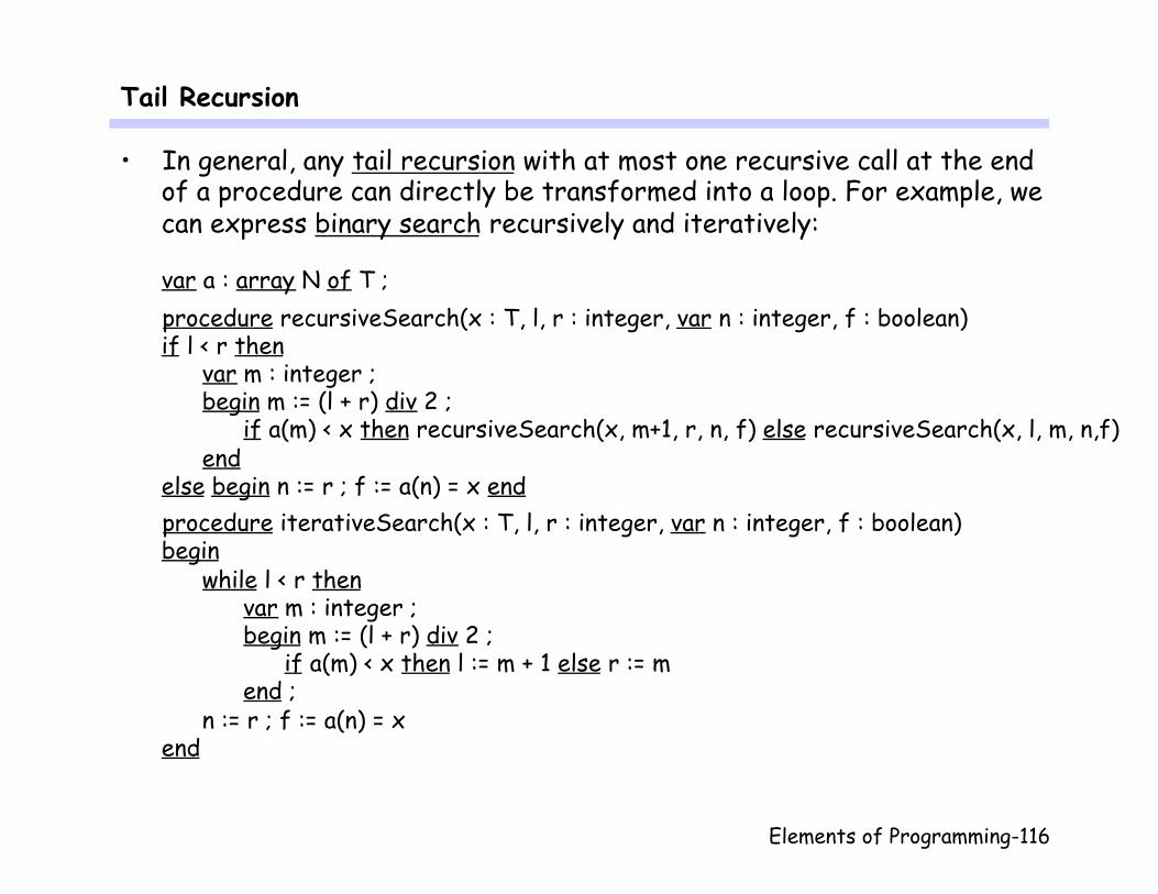
• In general, any tail recursion with at most one recursive call at the end of a procedure can directly be transformed into a loop. For example, we can express binary search recursively and iteratively:
var a : array N of T ; procedure recursiveSearch(x : T, l, r : integer, var n : integer, f : boolean) if l < r then
var m : integer ; begin m := (l + r) div 2 ; if a(m) < x then recursiveSearch(x, m+1, r, n, f) else recursiveSearch(x, l, m, n,f) end
else begin n := r ; f := a(n) = x end procedure iterativeSearch(x : T, l, r : integer, var n : integer, f : boolean) begin
while l < r then var m : integer ; begin m := (l + r) div 2 ; if a(m) < x then l := m + 1 else r := m end ; n := r ; f := a(n) = x
end

Elements of Programming-117
Verifying Recursive Procedures
• Both forms of binary search are verified by making – (∀ k | 0 ≤ k < l • a(k) < x) ∧ (∀ k | r ≤ k < N • a(k) ≥ x) ∧ (l ≤ r)
part of the invariant – r – l the bound
provided a is ascending, i.e. (∀ k | 0 < k < N • a(k – 1) ≤ a(k)). From the invariant we deduce that the first occurrence is found.
• In general, if P, Q are predicates, T an integer expression, the bound, v an auxiliary integer variable, procedure n has body S, and {P ∧ (T < v)} n {Q} ⇒ {P ∧ (T= v)} S {Q}
(under P body establishes Q and decreases T) {P ∧ (T ≤ 0)} S {Q} (T ≤ 0 causes termination) then
{P} n {Q} Show that the rule for repetition follows from this rule!
Elements of Programming-118
Quicksort – 1
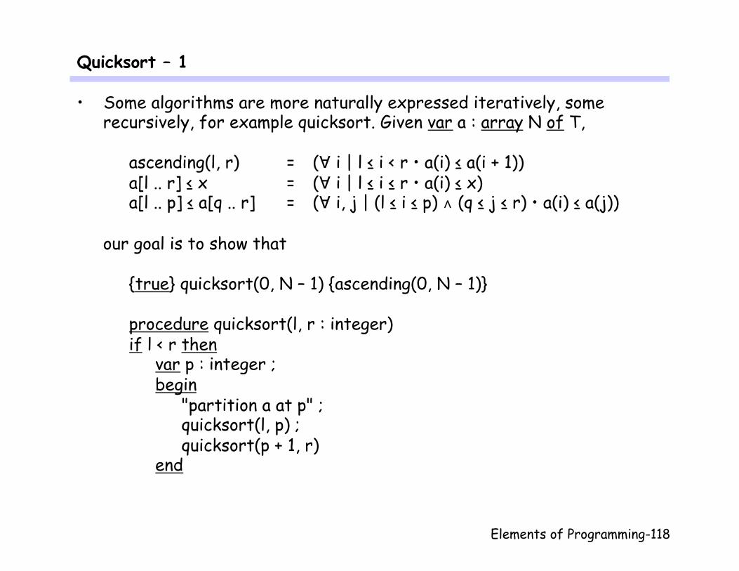
• Some algorithms are more naturally expressed iteratively, some recursively, for example quicksort. Given var a : array N of T,
ascending(l, r) = (∀ i | l ≤ i < r • a(i) ≤ a(i + 1)) a[l .. r] ≤ x = (∀ i | l ≤ i ≤ r • a(i) ≤ x) a[l .. p] ≤ a[q .. r] = (∀ i, j | (l ≤ i ≤ p) ∧ (q ≤ j ≤ r) • a(i) ≤ a(j))
our goal is to show that
{true} quicksort(0, N – 1) {ascending(0, N – 1)}
procedure quicksort(l, r : integer) if l < r then var p : integer ; begin "partition a at p" ; quicksort(l, p) ; quicksort(p + 1, r) end

Elements of Programming-119
Quicksort – 2
• The task of "partition a at p" is to move all smaller elements to the left of p and all larger element to right of p, and set p accordingly:
{l < r} "partition a at p" {(l ≤ p < r) ∧ (a[l .. p] ≤ a[p + 1 .. r])}
• We apply the rule for recursive procedures with the hypothesis that for the calls in the body of quicksort we can assume:
{true} quicksort(l, p) {ascending(l, p)} {true} quicksort(p + 1, r) {ascending(p + 1, r)}
From this we like to conclude that:
{true} if l < r then var p : integer ; begin … end {ascending(l, r)} This holds as (we do not go into the details here):
(l ≤ p < r) ∧ (a[l .. p] ≤ a[p + 1 .. r])) ∧ ascending(l, p) ∧ ascending(p + 1, r) ⇒ ascending(l, r)
Elements of Programming-120
Quicksort – 3
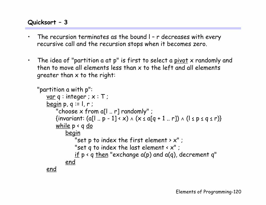
• The recursion terminates as the bound l – r decreases with every recursive call and the recursion stops when it becomes zero.
• The idea of "partition a at p" is first to select a pivot x randomly and then to move all elements less than x to the left and all elements greater than x to the right: "partition a with p":
var q : integer ; x : T ; begin p, q := l, r ; "choose x from a[l .. r] randomly" ; {invariant: (a[l .. p - 1] < x) ∧ (x ≤ a[q + 1 .. r]) ∧ (l ≤ p ≤ q ≤ r)} while p < q do begin "set p to index the first element > x" ; "set q to index the last element < x" ; if p < q then "exchange a(p) and a(q), decrement q" end end

Elements of Programming-121
Quicksort – 4
• "choose x from a[l .. r] randomly" can be refined in several ways: – Choose the first or last element: x := a(l) or x := a(r) – Choose the middle element: x := a((l + r) div 2)
The middle element yields the best behavior if the array is already ascending. We conclude with the complete program:
procedure quicksort(l, r : integer) if l < r then var p, q : integer ; x, h : T ; begin p, q := l, r ; x := a((l + r) div 2) ; while p < q do begin while a(p) < x do p := p + 1 ; while a(q) > x do q := q – 1 ; if p < q then begin h := a(p) ; a(p) := a(q) ; a(q) := h ; q := q – 1 end end ; quicksort(l, p) ; quicksort(p + 1, r) end

Elements of Programming-122
Assertions …
• The statement assert B does nothing if B holds and fails when B does not hold:
wp(assert B, P) = ∆ B ∧ B ∧ P
• Assert statements are used for documenting the intended use:
assert x ≥ 0 ; z, u := 0, x ; while u > 0 do z, u := z + y, u – 1 ; assert z = x · y
This states that if the program is executed with x < 0 initially, it fails; if finally z = x · y does not hold, it fails as well.
• We extend the syntax of statements accordingly:
statement ::= … | assert expression

Elements of Programming-123
… Assertions
• Assert statements are needed for restricting programs, for example:
procedure bookSeat begin assert seats < CAPACITY ; seat := seat + 1 end
procedure cancelSeat begin assert seats > 0 ; seat := seat – 1 end
• Note the difference between correctness assertions and assertion
statements: – Adding an assertion statement changes the meaning of a program. – A correctness assertion states a property of a program.
However, both are related:
{P} S {Q} = {P} assert P ; S ; assert Q {Q}
Elements of Programming-124
Using Assertions for Testing
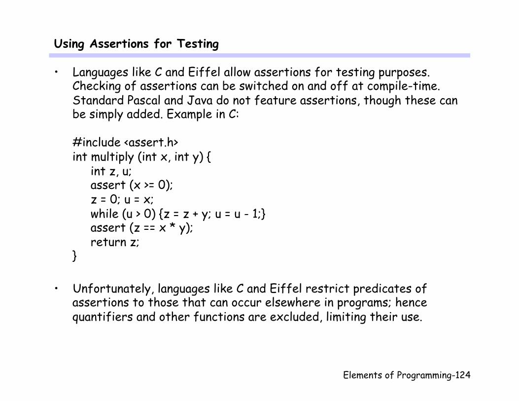
• Languages like C and Eiffel allow assertions for testing purposes. Checking of assertions can be switched on and off at compile-time. Standard Pascal and Java do not feature assertions, though these can be simply added. Example in C: #include <assert.h> int multiply (int x, int y) {
int z, u; assert (x >= 0); z = 0; u = x; while (u > 0) {z = z + y; u = u - 1;} assert (z == x * y); return z;
}
• Unfortunately, languages like C and Eiffel restrict predicates of assertions to those that can occur elsewhere in programs; hence quantifiers and other functions are excluded, limiting their use.

Elements of Programming-125
skip and abort …
• The statement skip does nothing, it is defined as assert true. The statement abort always fails, it is defined as assert false.
wp(skip, P) = P wp(abort, P) = false (In C and Java, skip is written as ";")
• We extend the syntax of statements accordingly: statement ::= …
| abort | skip
Elements of Programming-126
… skip and abort
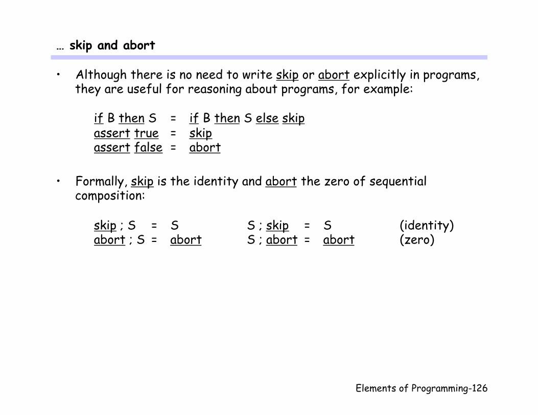
• Although there is no need to write skip or abort explicitly in programs, they are useful for reasoning about programs, for example:
if B then S = if B then S else skip assert true = skip assert false = abort
• Formally, skip is the identity and abort the zero of sequential
composition:
skip ; S = S S ; skip = S (identity) abort ; S = abort S ; abort = abort (zero)