notes on probability theory - hamilton institute
TRANSCRIPT

Notes on Probability Theory
Christopher King
Department of MathematicsNortheastern University
July 31, 2009
Abstract
These notes are intended to give a solid introduction to Proba-bility Theory with a reasonable level of mathematical rigor. Resultsare carefully stated, and many are proved. Numerous examples andexercises are included to illustrate the applications of the ideas. Manyimportant concepts are already evident in simple situations and thenotes include a review of elementary probability theory.
c© by Christopher K. King, 2009. All rights are reserved. These notesmay be reproduced in their entirety for non-commercial purposes.
1

Contents
1 Elementary probability 51.1 Why all the fuss? – can’t we just figure it out?? . . . . . . . . 51.2 Sample space . . . . . . . . . . . . . . . . . . . . . . . . . . . 61.3 Events . . . . . . . . . . . . . . . . . . . . . . . . . . . . . . . 71.4 Combining events . . . . . . . . . . . . . . . . . . . . . . . . . 71.5 Assigning probabilities . . . . . . . . . . . . . . . . . . . . . . 81.6 Drawing breath . . . . . . . . . . . . . . . . . . . . . . . . . . 101.7 Conditional probability . . . . . . . . . . . . . . . . . . . . . . 101.8 Independence . . . . . . . . . . . . . . . . . . . . . . . . . . . 121.9 Random variables . . . . . . . . . . . . . . . . . . . . . . . . . 131.10 Joint distributions . . . . . . . . . . . . . . . . . . . . . . . . 151.11 Expected value or expectation . . . . . . . . . . . . . . . . . . 161.12 Draw breath again . . . . . . . . . . . . . . . . . . . . . . . . 171.13 Function of a random variable . . . . . . . . . . . . . . . . . . 171.14 Moments of X . . . . . . . . . . . . . . . . . . . . . . . . . . . 191.15 Function of a random vector . . . . . . . . . . . . . . . . . . . 201.16 Conditional distribution and expectation . . . . . . . . . . . . 21
2 Discrete-time finite state Markov chains 242.1 Definition of the chain . . . . . . . . . . . . . . . . . . . . . . 242.2 Absorbing chains . . . . . . . . . . . . . . . . . . . . . . . . . 272.3 Ergodic Markov chains . . . . . . . . . . . . . . . . . . . . . . 322.4 Classification of finite-state Markov chains . . . . . . . . . . . 41
3 Existence of Markov Chains 433.1 Sample space for Markov chain . . . . . . . . . . . . . . . . . 433.2 Lebesgue measure . . . . . . . . . . . . . . . . . . . . . . . . . 45
4 Discrete-time Markov chains with countable state space 464.1 Some motivating examples . . . . . . . . . . . . . . . . . . . . 464.2 Classification of states . . . . . . . . . . . . . . . . . . . . . . 474.3 Classification of Markov chains . . . . . . . . . . . . . . . . . 484.4 Time reversible Markov chains . . . . . . . . . . . . . . . . . . 56
2

5 Probability triples 585.1 Rules of the road . . . . . . . . . . . . . . . . . . . . . . . . . 585.2 Uncountable sample spaces . . . . . . . . . . . . . . . . . . . . 585.3 σ-algebras . . . . . . . . . . . . . . . . . . . . . . . . . . . . . 595.4 Continuity . . . . . . . . . . . . . . . . . . . . . . . . . . . . . 615.5 Draw breath . . . . . . . . . . . . . . . . . . . . . . . . . . . . 625.6 σ-algebra generated by a class . . . . . . . . . . . . . . . . . . 645.7 Borel sets . . . . . . . . . . . . . . . . . . . . . . . . . . . . . 655.8 Lebesgue measure . . . . . . . . . . . . . . . . . . . . . . . . . 665.9 Lebesgue-Stieltjes measure . . . . . . . . . . . . . . . . . . . . 685.10 Lebesgue-Stieltjes measure on Rn . . . . . . . . . . . . . . . . 695.11 Random variables . . . . . . . . . . . . . . . . . . . . . . . . . 695.12 Continuous random variables . . . . . . . . . . . . . . . . . . 715.13 Several random variables . . . . . . . . . . . . . . . . . . . . . 745.14 Independence . . . . . . . . . . . . . . . . . . . . . . . . . . . 745.15 Expectations . . . . . . . . . . . . . . . . . . . . . . . . . . . 755.16 Calculations with continuous random variables . . . . . . . . . 785.17 Stochastic processes . . . . . . . . . . . . . . . . . . . . . . . . 81
6 Limit Theorems for stochastic sequences 836.1 Basics about means and variances . . . . . . . . . . . . . . . . 836.2 Review of sequences: numbers and events . . . . . . . . . . . . 836.3 The Borel-Cantelli Lemmas and the 0− 1 Law . . . . . . . . . 876.4 Some inequalities . . . . . . . . . . . . . . . . . . . . . . . . . 896.5 Modes of convergence . . . . . . . . . . . . . . . . . . . . . . . 906.6 Weak law of large numbers . . . . . . . . . . . . . . . . . . . . 926.7 Strong law of large numbers . . . . . . . . . . . . . . . . . . . 936.8 Applications of the Strong Law . . . . . . . . . . . . . . . . . 95
7 Moment Generating Function 977.1 Moments of X . . . . . . . . . . . . . . . . . . . . . . . . . . . 977.2 Moment Generating Functions . . . . . . . . . . . . . . . . . . 97
8 The Central Limit Theorem 1018.1 Applications of CLT . . . . . . . . . . . . . . . . . . . . . . . 1038.2 Rate of convergence in LLN . . . . . . . . . . . . . . . . . . . 104
3

9 Measure Theory 1069.1 Extension Theorem . . . . . . . . . . . . . . . . . . . . . . . . 1069.2 The Lebesgue measure . . . . . . . . . . . . . . . . . . . . . . 1119.3 Independent sequences . . . . . . . . . . . . . . . . . . . . . . 1129.4 Product measure . . . . . . . . . . . . . . . . . . . . . . . . . 112
10 Applications 11310.1 Google Page Rank . . . . . . . . . . . . . . . . . . . . . . . . 11310.2 Music generation . . . . . . . . . . . . . . . . . . . . . . . . . 11610.3 Bayesian inference and Maximum entropy principle . . . . . . 117
10.3.1 Example: locating a segment . . . . . . . . . . . . . . 11710.3.2 Maximum entropy rule . . . . . . . . . . . . . . . . . . 11810.3.3 Back to example . . . . . . . . . . . . . . . . . . . . . 118
10.4 Hidden Markov models . . . . . . . . . . . . . . . . . . . . . . 12010.4.1 The cheating casino . . . . . . . . . . . . . . . . . . . . 12010.4.2 Formal definition . . . . . . . . . . . . . . . . . . . . . 12010.4.3 Applications . . . . . . . . . . . . . . . . . . . . . . . . 12110.4.4 The forward-backward procedure . . . . . . . . . . . . 12110.4.5 Viterbi algorithm . . . . . . . . . . . . . . . . . . . . . 122
4

1 Elementary probability
Many important concepts are already evident in simple situations so we startwith a review of elementary probability theory.
1.1 Why all the fuss? – can’t we just figure it out??
Questions in probability can be tricky, and we benefit from a clear under-standing of how to set up the solution to a problem (even if we can’t solveit!). Here is an example where intuition may need to be helped along a bit:
“Remove all cards except aces and kings from a deck, so that only eightcards remain, of which four are aces and four are kings. From this abbreviateddeck, deal two cards to a friend. If he looks at his card and announces(truthfully) that his hand contains an ace, what is the probability that bothhis cards are aces? If he announces instead that one of his cards is the ace ofspades, what is the probability then that both his cards are aces? Are thesetwo probabilities the same?”
Probability theory provides the tools to organize our thinking about howto set up calculations like this. It does this by separating out the two impor-tant ingredients, namely events (which are collections of possible outcomes)and probabilities (which are numbers assigned to events). This separationinto two logically distinct camps is the key which lets us think clearly aboutsuch problems. For example, in the first case above, we ask “which outcomesmake such an event possible?”. Once this has been done we then figure outhow to assign a probability to the event (for this example it is just a ratio ofintegers, but often it is more complicated).
First case: there are 28 possible ‘hands’ that can be dealt (choose 2 cardsout of 8). Out of these 28 hands, exactly 6 contain no aces (choose 2 cardsout of 4). Hence 28-6=22 contain at least one ace. Our friend tells us he hasan ace, hence he has been dealt one of these 22 hands. Out of these exactly6 contain two aces (again choose 2 out of 4). Therefore he has a probabilityof 6/22=3/11 of having two aces.
Second case: one of his cards is the ace of spades. There are 7 possibilitiesfor the other card, out of which 3 will yield a hand with 2 aces. Thus theprobability is 3/7.
Any implicit assumptions?? Yes: we assume all hands are equally likely.
5

1.2 Sample space
The basic setting for a probability model is the random experiment or randomtrial. This is your mental model of what is going on. In our previous examplethis would be the dealer passing over two cards to your friend.
Definition 1 The sample space S is the set of all possible outcomes of therandom experiment.
Depending on the random experiment, S may be finite, countably infiniteor uncountably infinite. For a random coin toss, S = H,T, so |S| = 2. Forour card example, |S| = 28, and consists of all possible unordered pairs ofcards, eg (Ace of Hearts, King of Spades) etc. But note that you have somechoice here: you could decide to include the order in which two cards aredealt. Your sample space would then be twice as large, and would includeboth (Ace of Hearts, King of Spades) and (King of Spades, Ace of Hearts).Both of these are valid sample spaces for the experiment. So you get the firsthint that there is some artistry in probability theory! namely how to choosethe ‘best’ sample space.
Other examples:
(1) Roll a die: the outcome is the number on the upturned face, so S =1, 2, 3, 4, 5, 6, |S| = 6.
(2) Toss a coin until Heads appears: the outcome is the number of tossesrequired, so S = 1, 2, 3, . . . , |S| =∞.
(3) Choose a random number between 0 and 1: S = [0, 1]. (This is thefirst example of an uncountable sample space).
(4) Throw a dart at a circular dartboard:
S = (x, y) ∈ R2 |x2 + y2 ≤ 1
For this review of elementary probability we will restrict ourselves to finiteand countably infinite sample spaces.
6
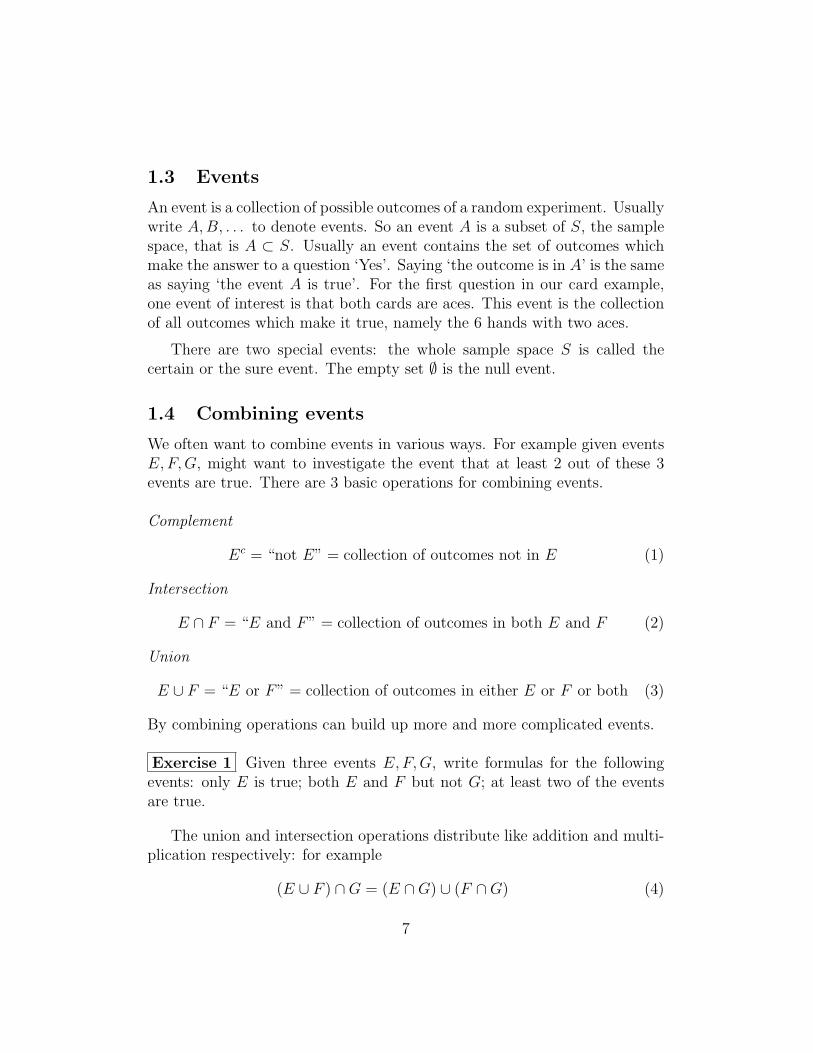
1.3 Events
An event is a collection of possible outcomes of a random experiment. Usuallywrite A,B, . . . to denote events. So an event A is a subset of S, the samplespace, that is A ⊂ S. Usually an event contains the set of outcomes whichmake the answer to a question ‘Yes’. Saying ‘the outcome is in A’ is the sameas saying ‘the event A is true’. For the first question in our card example,one event of interest is that both cards are aces. This event is the collectionof all outcomes which make it true, namely the 6 hands with two aces.
There are two special events: the whole sample space S is called thecertain or the sure event. The empty set ∅ is the null event.
1.4 Combining events
We often want to combine events in various ways. For example given eventsE,F,G, might want to investigate the event that at least 2 out of these 3events are true. There are 3 basic operations for combining events.
Complement
Ec = “not E” = collection of outcomes not in E (1)
Intersection
E ∩ F = “E and F” = collection of outcomes in both E and F (2)
Union
E ∪ F = “E or F” = collection of outcomes in either E or F or both (3)
By combining operations can build up more and more complicated events.
Exercise 1 Given three events E,F,G, write formulas for the followingevents: only E is true; both E and F but not G; at least two of the eventsare true.
The union and intersection operations distribute like addition and multi-plication respectively: for example
(E ∪ F ) ∩G = (E ∩G) ∪ (F ∩G) (4)
7

The complement squares to the identity: (Ec)c = E. De Morgan’s Laws are
(E ∩ F )c = Ec ∪ F c, (E ∪ F )c = Ec ∩ F c (5)
Exercise 2 Circuit with switches in parallel or in series. Describe eventthat circuit is open in terms of events that each switch is open or closed.
1.5 Assigning probabilities
The second ingredient in our setup is the assignment of a probability toan event. These probabilities can often be calculated from ‘first principles’.In our card example we did this by counting and dividing. In other casesthe probabilities may be given as part of the description of the problem; forexample if you are told that a coin is biased and comes up Heads twice as oftenas Tails. We next analyze the requirements for a satisfactory assignment.
The basic step is that every event E is assigned a probability P (E). Thisis a number satisfying
0 ≤ P (E) ≤ 1 (6)
The meaning is “P (E) is the probability that event E is true”. The oper-ational meaning (which will follow from the mathematical setup) is that ifthe random experiment (our mental image of the process) is repeated manytimes under identical conditions, then in the long-run the fraction of timeswhen E is true will approach P (E) as the number of trials becomes arbitrar-ily large. Since this can never be checked in practice, it remains an article offaith about how the universe works. Nevertheless it can be formulated as amathematical statement in probability theory, and then it can be shown tobe a consequence of the axioms of the theory. This result is called the Lawof Large Numbers and will be studied in detail later in the course.
There are lots of possible events, so there are consistency relations thatmust be satisfied. Here are some:
(1) P (Ec) = 1− P (E)
(2) P (S) = 1
8

(3) if E ⊂ F then P (E) ≤ P (F )
(4) if E ∩ F = ∅ (aka E and F are disjoint, or mutually exclusive), then
P (E ∪ F ) = P (E) + P (F ) (7)
(5) for any events E,F ,
P (E ∪ F ) = P (E) + P (F )− P (E ∩ F ) (8)
(6) if E1, E2, . . . , En, . . . is a sequence of pairwise disjoint events, so thatEi ∩ Ej = ∅ for all i 6= j, then
P (∞⋃n=1
En) =∞∑n=1
P (En) (9)
The last property (6) is crucial, and it cannot be deduced from the pre-vious relations which involve only finitely many sets. This property is calledcountable additivity and we will have much more to say about it later.
Other relations then follow from these. However it can be shown thatthere are no other independent relations; if conditions (1) – (6) hold for allevents then P is a consistent assignment of probabilities on S. In this casethe assignment P is called a probability model or probability law on S.
Some work has gone into finding a minimal set of relations which generateall others: one such minimal set is the two relations (2) and (6) above.
Exercise 3 Derive (1), (3), (5) from (2) and (4).
Exercise 4 Two events E and F ; the probability that neither is true is 0.6,the probability that both are true is 0.2; find the probability that exactly oneof E or F is true.
In elementary probability theory where S is either finite or countablyinfinite, every possible outcome s ∈ S is assigned a probability p(s), andthen the probability of any event A can be calculated by the sum
P (A) =∑s∈A
p(s) (10)
9

This relation follows from (6) above, since A = ∪s∈As is a countable unionof disjoint sets. The sum always converges, even if S is (countably) infi-nite. Furthermore, if p : S → [0, 1], s 7→ p(s) is any map that satisfies thecondition ∑
s∈S
p(s) = 1 (11)
then it defines a probability law on S.
Exercise 5 For any sequence of events An, use Property (6) to showthat
P (∞⋃n=1
An) ≤∞∑n=1
P (An) (12)
[Hint: rewrite⋃∞n=1An as a union of pairwise disjoint sets]
1.6 Drawing breath
To summarize: we have laid down the mathematical foundations of prob-ability theory. The key step is to recognize the two separate pillars of thesubject, namely on the one hand the sample space of outcomes, and on theother hand the numerical probabilities which are assigned to events. Nextwe use this basic setup to define the familiar notions of probability, such asindependence, random variables etc..
1.7 Conditional probability
P (B|A) = conditional probability that B is true given that A is true
Imagine the following 2-step thought experiment: you toss a coin; if it comesup Heads, you draw one card at random from a standard deck; if it comesup Tails you draw two cards at random (without replacement). Let A bethe event that you get Heads on the coin toss, and let B be the event thatyou draw at least one Ace from the deck. Then P (B|A) is clearly 4/52 =1/13. What about P (A ∩ B)? Imagine lining up all your many repeatedexperiments, then for approximately one-half of them the event A will be
10

true. Out of these approximately 1/13 will have B also true. So we expectthat P (A ∩ B) = (1/2)(1/13) = P (A)P (B|A). This line of reasoning leadsto the following definition:
P (B|A) =P (B ∩ A)
P (A)(13)
It is important to note that P (B|A) is defined only if P (A) 6= 0.
Exercise 6 Suppose that P (B|A) > P (B). What does this imply aboutthe relation between P (A|B) and P (A)?
Exercise 7 Show that
P (A1 ∩ A2 ∩ · · · ∩ An)
= P (A1)P (A2|A1)P (A3|A1 ∩ A2) . . . P (An|A1 ∩ A2 ∩ · · · ∩ An−1) (14)
Exercise 8 A standard deck of 52 playing cards is randomly divided into4 piles of 13 cards each. Find the probability that each pile has exactly oneAce.[Hint: define events A1, . . . , A4 by
Ak = the kth pile has exactly one Ace, k = 1, 2, 3, 4 (15)
and use the previous Exercise]
One useful application is the formula for total probability: suppose thatthere is a collection of events A1, A2, . . . , An which are mutually disjoint, soAi ∩ Aj = ∅ for all i 6= j, and also exhaustive, meaning they include everyoutcome so that A1 ∪ A2 ∪ · · · ∪ An = S. Then for any event B,
P (B) = P (B ∩ A1) + P (B ∩ A2) + · · ·+ P (B ∩ An)
= P (B|A1)P (A1) + P (B|A2)P (A2) + · · ·+ P (B|An)P (An)(16)
Note that the first equality follows from Property (4) of the probability law.
11

Exercise 9 Derive Bayes formula: for mutually exclusive and exhaustiveevents A1, . . . , An,
P (Ai|B) =P (B|Ai)P (Ai)
P (B|A1)P (A1) + P (B|A2)P (A2) + · · ·+ P (B|An)P (An)(17)
Exercise 10 A patient walks in who has a fever and chills. The doctorwonders, “what is the chance that this patient has tuberculosis given thesymptoms I am seeing?” Let A be the event that the patient has TB, letB be the event that the patient has fever and chills. Assume that TB ispresent in 0.01% of the population, whereas 3% of the population exhibitsfever and chills. Assume that P (B|A) = 0.5. What is the answer to thedoctor’s question?
Exercise 11 Rework our old card problem using conditional probabilities.
1.8 Independence
Two events A,B are independent if
P (A|B) = P (A)⇐⇒ P (B|A) = P (B)⇐⇒ P (A ∩B) = P (A)P (B) (18)
In other words these three conditions are equivalent.The collection of events A1, . . . , An, . . . is independent if for every finite
subset Ai1 , . . . , Aik ,
P (Ai1 ∩ · · · ∩ Aik) = P (Ai1) · · ·P (Aik) (19)
Independence is very important in probability theory because it occursnaturally in many applications, and also because it provides very useful toolsfor solving problems.
Exercise 12 Successive coin tosses are independent. A biased coin hasprobability p of coming up Heads. The coin is tossed 10 times. Find theprobability that it comes up Heads at least twice.
Exercise 13 Two dice are rolled many times, and each time the sum ofthe numbers on the dice is recorded. Find the probability that the value 8will occur before the value 7.
12

1.9 Random variables
A random variable is a ‘random number’, meaning a number which is deter-mined by the outcome of a random experiment. Usually denoted X, Y, . . . .The range of X is the set of possible values for X. Mathematically, X is areal-valued map on the sample space S:
X : S → R, s 7→ X(s) (20)
Another way to say this is that X is the result of a measurement of intereston S.
In elementary probability we consider only discrete random variableswhose range is either finite or countably infinite. If the range of X is finitethen we say that X is a simple random variable. The event X = x is theset of outcomes in S for which the value x is assigned to X. Mathematically,
X = x = s ∈ S |X(s) = x = X−1(x) (21)
The probability of this event is written P (X = x). At this point thesample space S recedes into the background, and we can concentrate just onthe range of possible values of X and their probabilities. This list is calledthe probability mass function or pmf of X:
(x1, p1), (x2, p2), . . . (22)
where Ran(X) = x1, x2, . . . and pk = P (X = xk).
Exercise 14 Roll two fair dice, Y is the maximum of the two numbers ontheir faces, find the pmf of Y .
Given just the pmf of X, is there a unique underlying sample space Swith its probability assignments? The answer is no. There are many samplespaces which would yield the same pmf for X. But there is a minimal samplespace which does the job. Just take S to be the set of points in the rangeof X, and assign probabilities to these points according to the pmf of X.So S = x1, x2, . . . and P (xk) = pk. In this case the map which definesX is particularly simple, it is just the identity function: X(xk) = xk. Thisexercise also shows that there is a random variable defined for every pmf:given a countable set of real numbers xk and a set of probabilities pksatisfying
∑k pk = 1, there is a random variable X whose pmf is (xk, pk).
13

To see an example, suppose we roll two fair dice and define
X =
0 if the dice are different
1 if the dice are the same
The obvious sample space has 36 elements, namely all pairs of outcomesfor the dice. The map X assigns value either 0 or 1 to every outcome, e.g.X(1, 3) = 0, X(4, 4) = 1, etc. The pmf of X is
P (X = 0) =1
6, P (X = 1) =
5
6
We could instead take our sample space to consist of just two elements,namely S = 0, 1 with probabilities (1/6, 5/6), then define X(0) = 0 andX(1) = 1, and we end up with the same pmf for X. So all that really mattersfor X is that it is possible to construct a sample space on which X can bedefined with this pmf, we don’t actually care about the details of the samplespace.
There are several special discrete random variables which are especiallyimportant because they arise in many situations.
BernoulliRan(X) = 0, 1, p = P (X = 1), 1− p = P (X = 0). For example, a biasedcoin has probability p of coming up Heads. Toss coin, X is number of Heads.
Binomial
Ran(X) = 0, 1, 2, . . . , n, P (X = k) =
(nk
)pk(1−p)n−k. Now X is number
of Heads for n tosses of a biased coin. As a shorthand write
X ∼ Bin(n, p) (23)
PoissonRan(X) = 0, 1, 2, . . . , P (X = k) = e−λ λk
k!. For example, X counts number
of occurrences of rare events, like radioactive decays from a sample.
There is an important relation between the Binomial and Poisson formu-las.
Lemma 2 Fix λ = np, then
limn→∞, p→0
(nk
)pk(1− p)n−k = e−λ
λk
k!
14

Exercise 15 Biased coin, p is probability of Heads. Toss coin until Headsappears. Let N be number of tosses, find the pmf of N . [This is the geometricdistribution].
1.10 Joint distributions
In many circumstances we encounter a collection of random variables whichare all related to each other. For example, X and Y could be the minimumand maximum respectively of two rolls of the dice. Often we want to considerthese related random variables together.
Given a collection of discrete random variables X = (X1, X2, . . . , Xn),let Ri be the range of Xi. Then the range of X is the Cartesian productR1 × · · · × Rn. Their joint pmf is the collection of probabilities P (X1 =x1, . . . , Xn = xn) for every point (x1, . . . , xn) in the range of X1, X2, . . . , Xn.It is also convenient to view X as a random vector in Rn.
Exercise 16 Let X and Y be the minimum and maximum respectively oftwo rolls of the dice. Find the joint pmf of X and Y .
The random variables X1, X2, . . . , Xn are defined on the same samplespace S. Just as for a single discrete random variable, if S is not known apriori we can always construct a sample space for X1, X2, . . . , Xn by takingS to be the range R1×· · ·×Rn, and defining the probability of a point usingthe pmf. Then Xi is the projection onto the ith coordinate.
We can recover the pmf of X1 by itself from the joint pmf:
P (X1 = x1) =∑
x2,...,xn
P (X1 = x1, X2 = x2, . . . , Xn = xn) (24)
This procedure is called finding the marginal pmf of X1. The same procedureworks for X2, . . . , Xn.
The random variables X1, X2, . . . , Xn are independent if for every point(x1, . . . , xn) the events X1 = x1, X2 = x2, . . . , Xn = xn are indepen-dent. Equivalently, X1, X2, . . . , Xn are independent if and only if the jointpmf is the product of the marginals, that is for every point (x1, . . . , xn),
P (X1 = x1, . . . , Xn = xn) = P (X1 = x1) . . . P (Xn = xn) (25)
15

Exercise 17 You have two coins, one is unbiased, the other is biased withprobability of Heads equal to 2/3. You toss both coins twice, X is the numberof Heads for the fair coin, Y is the number of Heads for the biased coin. FindP (X > Y ). [Hint: X and Y are independent].
Exercise 18 Two biased coins have the same probability p of coming upHeads. The first coin is tossed until Heads appears for the first time, let Nbe the number of tosses. The second coin is then tossed N times. Let X bethe number of times the second coin comes up Heads. Find the pmf of X(express the pmf by writing P (X = k) as an infinite series).
1.11 Expected value or expectation
Let X be a discrete random variable with pmf (x1, p1), (x2, p2), . . . . If therange of X is finite the expected value or expectation of X is defined to be
EX =∑n
pnxn (26)
As an example can compute expected value of roll of die (= 7/2).
If the range of X is infinite, the sum is defined as follows: first divide Xinto its positive and negative parts X+ and X−,
X+ = maxX, 0, X− = X −X+ (27)
Define
EX+ =∑
n :xn≥0
pnxn, EX− =∑
n :xn<0
pn|xn| (28)
Both are sums of positive terms, hence each either converges or is +∞. Unlessboth EX+ = EX− = +∞ we say that EX exists and define it to be
EX = EX+ − EX− (29)
The value of EX may be finite, or ±∞. If both EX+ = EX− = +∞ thenEX does not exist. Note that |X| = X+ +X−. Hence EX exists and is finiteif and only if E|X| exists and is finite.
EX has a nice operational meaning. Repeat the underlying random ex-periment many times, and measure the value of X each time. Let Av(X;n)
16

be the average of these values for n successive measurements. This averagevalue depends on n and is itself a random variable. However our experiencewith the universe shows that Av(X;n) converges as n→∞, and this limit-ing value is EX. Again this can never be verified by experiment but it canbe derived mathematically from the axioms.
Exercise 19 Find EX when: (a) X is maximum of two dice rolls (=161/36), (b)X is number of tosses of biased coin until Heads first appears(= 1/p).
1.12 Draw breath again
We have now met all the ingredients of elementary probability theory. Withthese in hand you can tackle any problem involving finite sample spaces anddiscrete random variables. We will shortly look in detail at one such class ofmodels, namely finite state Markov chains. First we consider some furthertechnical questions.
1.13 Function of a random variable
Let X : S → R be a discrete random variable, and g : R → R a real-valuedfunction. Then Y = g X : S → R is also a random variable. Its range is
Ran(Y ) = g(Ran(X)) = g(xk) |xk ∈ Ran(X) (30)
and its pmf is
P (Y = y) = P (s : g(X(s)) = y)=
∑s : g(X(s))=y
p(s)
=∑
k:g(xk)=y
∑s :X(s)=xk
p(s)
=∑
k:g(xk)=y
P (X = xk) (31)
Write Y = g(X). To compute EY , first define the positive and negative
17

parts Y + and Y − as before. Then
EY + =∑yj≥0
yjP (Y = yj)
=∑yj≥0
yj∑
k:g(xk)=yj
P (X = xk)
=∑yj≥0
∑k:g(xk)=yj
g(xk)P (X = xk)
=∑yj≥0
∑k
1g(xk)=yj g(xk)P (X = xk) (32)
where 1A is the indicator function of the event A: it equals 1 if A is true, and0 if false. All terms in the double summation are positive, so we can changethe order of summation without changing the value of the sum. Hence
EY + =∑k
∑yj≥0
1g(xk)=yj g(xk)P (X = xk)
=∑
k:g(xk)≥0
g(xk)P (X = xk) (33)
The same calculation shows that
EY − =∑
k:g(xk)<0
g(xk)P (X = xk) (34)
Assuming EY is defined, so at least one of EY + and EY − is finite, we concludethat
EY =∑k
g(xk)P (X = xk) (35)
or more casually
Eg(X) =∑x
g(x)P (X = x) (36)
This is a change of variables formula which allows us to compute expectationsof functions of X directly from the pmf of X itself.
18

Exercise 20 Suppose ai,j ≥ 0 for all i, j ≥ 1, show that
∞∑i=1
( ∞∑j=1
ai,j
)=∞∑j=1
( ∞∑i=1
ai,j
)(37)
where +∞ is a possible value for both sums.
Exercise 21 Show that E[·] is a linear operator.
Exercise 22 If Ran(N) = 1, 2, . . . show that
EN =∞∑n=1
P (N ≥ n) (38)
Exercise 23 Compute EX2 where X is the number of tosses of a biasedcoin until Heads first appears (= (2− p)/p2).
1.14 Moments of X
The kth moment of X is defined to be EXk (if it exists). The first momentis the expected value of X, also called the mean of X.
Exercise 24 If the kth moment of X exists and is finite, show that the jth
moment exists and is finite for all 1 ≤ j ≤ k. [Hint: if j ≤ k show that|X|j ≤ 1 + |X|k]
The variance of X is defined to be
VAR(X) = E(X − EX
)2
(39)
If the second moment of X exists then
VAR(X) = E[X2 − 2XEX + (EX)2] = EX2 − (EX)2 (40)
The standard deviation of X is defined as
STD(X) =√
VAR(X) (41)
19

Exercise 25 Suppose Ran(X) = 1, 2, . . . and P (X = k) = c k−t wheret > 1 and c > 0 is an irrelevant constant. Find which moments of X arefinite (the answer depends on t).
The moment generating function (mgf) of X is defined for t ∈ R by
MX(t) = EetX =∑x
etxP (X = x) (42)
If X is finite then MX always exists. If X is infinite it may or may not existfor a given value t. Since etx > 0 for all t, x, the mgf is either finite or +∞.Clearly MX(0) = 1.
1.15 Function of a random vector
Suppose X1, . . . , Xn are random variables with joint pmf p(x1, . . . , xn). Letg : Rn 7→ R, then
Eg(X1, . . . , Xn) =∑
x1,...,xn
g(x1, . . . , xn) p(x1, . . . , xn) (43)
In particular if g(x1, . . . , xn) = xk is the projection onto the kth coordinatethen
Eg(X1, . . . , Xn) = EXk =∑
x1,...,xn
xk p(x1, . . . , xn) =∑xk
xk p(xk) (44)
where p(xk) = P (X = xk) is the marginal pmf of Xk.
Commonly encountered applications of this formula include:
E(aX + bY ) = aEX + bEY (45)
COV(X, Y ) = E(X − EX)(Y − EY ) = E(XY )− (EX)(EY ) (46)
The last number is the covariance if X and Y and it measures the degree ofdependence between the two random variables.
Exercise 26 If X and Y are independent show that COV(X, Y ) = 0.
20

Exercise 27 Calculate COV(X, Y ) when X, Y are respectively the maxand min of two dice rolls.
As noted above, if X and Y are independent then COV(X, Y ) = 0, thatis E(XY ) = (EX)(EY ). Application of this and a little algebra shows thatif X1, X2, . . . , Xn are all independent, then
VAR[X1 +X2 + · · ·+Xn] = VAR[X1] + VAR[X2] + · · ·+ VAR[Xn] (47)
Exercise 28 Using the linearity of expected value and the above propertyof variance of a sum of independent random variables, calculate the mean andvariance of the binomial random variable. [Hint: write X = X1 + · · · + Xn
where Xk counts the number of Heads on the kth toss].
Exercise 29 Derive the formula
VAR[X1 +X2 + · · ·+Xn] =n∑k=1
VAR[Xk] + 2∑i<j
COV(Xi, Xj) (48)
1.16 Conditional distribution and expectation
If two random variables are independent then knowing the value of one ofthem tells you nothing about the other. However if they are dependent, thenknowledge of one gives you information about the likely value of the other.Let X, Y be discrete random variables. The conditional distribution of Xconditioned on the event Y = y is (assuming P (Y = y) 6= 0)
P (X = x |Y = y) =P (X = x , Y = y)
P (Y = y)
For a non-negative random variable X and an event A with P (A) 6= 0,define the conditional expectation of X with respect to A as
E[X|A] =∑x
xP (X = x|A) (49)
21

Since all terms in the sum are positive, either the sum converges or else it is+∞. For a general random variable X, write X = X+−X− and then define
E[X|A] = E[X+|A]− E[X−|A] (50)
assuming as usual that both terms are not infinite.An important special case is where A = Y = y for some random
variable Y , with P (Y = y) 6= 0. Since E[X|Y = y] is defined for everyy ∈ Ran(Y ), it defines a real-valued function on S, and hence is itself arandom variable. It is denoted E[X|Y ] and is defined by
E[X|Y ] : S → R, s 7→ E[X|Y = Y (s)] (51)
Since the value of E[X|Y ](s) depends only on Y (s), it follows that E[X|Y ] isa function of Y . Hence its expected value can be computed using our formulafor expectation of a function of a random variable:
E[E[X|Y ]] =∑y
E[X|Y = y]P (Y = y) (52)
Exercise 30 Assuming that EX exists, show that
E[E[X|Y ]] = EX (53)
Exercise 31 Let N,X1, X2, . . . be independent random variables on a dis-crete sample space S. Assume the Xk are identically distributed with finitemean EXk = µ. Also assume that Ran(N) = 1, 2, 3, . . . = N, and thatEN <∞. Define
Y =N∑n=1
Xn (54)
Prove that EY = µEN .
Exercise 32 Same setup as in previous exercise, assume in addition thatboth VAR[Xk] <∞ and VAR[N ] <∞. Prove that
VAR[Y ] = EN VAR[X] + µ2 VAR[N ] (55)
22

Exercise 33 A rat is trapped in a maze with three doors. Door #1 leadsto the exit after 1 minute. Door #2 returns to the maze after three minutes.Door #3 returns to the maze after five minutes. Assuming that the rat is atall times equally likely to choose any one of the doors, what is the expectedlength of time until the rat reaches the exit?
23

2 Discrete-time finite state Markov chains
Now we can ‘get moving’ with the Markov chain. This is the simplest non-trivial example of a stochastic process. It has an enormous range of applica-tions, including:
• statistical physics
• queueing theory
• communication networks
• voice recognition
• bioinformatics
• Google’s pagerank algorithm
• computer learning and inference
• economics
• gambling
• data compression
2.1 Definition of the chain
Let S = 1, . . . , N. A collection of S-valued random variables X0, X1, X2, . . . is called a discrete-time Markov chain on S if it satisfies the Markov condi-tion:
P (Xn = j |X0 = i0, . . . , Xn−1 = in−1) = P (Xn = j |Xn−1 = in−1) (56)
for all n ≥ 1 and all states j, i0, . . . , in−1 ∈ S.Regarding the index of Xn as a discrete time the Markov condition can be
summarized by saying that the conditional distribution of the present stateXn conditioned on the past states X0, . . . , Xn−1 is equal to the conditionaldistribution of Xn conditioned on the most recent past state Xn−1. In otherwords, the future (random) behavior of the chain only depends on where thechain sits right now, and not on how it got to its present position.
24

We will mostly consider homogeneous chains, meaning that for all n andi, j ∈ S
P (Xn = j |Xn−1 = i) = P (X1 = j |X0 = i) = pij (57)
This defines the N ×N transition matrix P with entries pij.A transition matrix must satisfy these properties:
(P1) pij ≥ 0 for all i, j ∈ S
(P2)∑
j∈S pij = 1 for all i ∈ S
Such a matrix is also called row-stochastic. So a square matrix is a transitionmatrix if and only if it is row-stochastic.
Once the initial probability distribution of X0 is specified, the joint dis-tribution of the Xi is determined. So let αi = P (X0 = i) for all i ∈ S, thenfor any sequence of states i0, i1, . . . , im we have (recall Exercise **)
P (X0 = i0, X1 = i1, . . . , Xm = im) = αi0pi0,i1pi1,i2 . . . pim−1,im (58)
The transition matrix contains the information about how the chainevolves over successive transitions. For example,
P (X2 = j|X0 = i) =∑k
P (X2 = j,X1 = k|X0 = i)
=∑k
P (X2 = j|X1 = k,X0 = i)P (X1 = k|X0 = i)
=∑k
P (X2 = j|X1 = k)P (X1 = k|X0 = i)
=∑k
pkj pik
=∑k
(P )ik (P )kj
= (P 2)ij (59)
So the matrix P 2 provides the transition rule for two consecutive steps of thechain. It is easy to check that P 2 is also row-stochastic, and hence is the tran-sition matrix for a Markov chain, namely the two-step chain X0, X2, X4, . . . ,or X1, X3, . . . . A similar calculation shows that for any k ≥ 1
P (Xk = j|X0 = i) = (P k)ij (60)
25

and hence P k is the k-step transition matrix. We write
pij(n) = (P n)ij = P (Xn = j|X0 = i) (61)
Note that pij = 0 means that the chain cannot move from state i to state jin one step. However it is possible in this situation that there is an integern such that pij(n) > 0, meaning that it is possible to move from i to j in nsteps. In this case we say that state j is accessible from state i.Example 1
Consider the following model. There are four balls, two White and twoBlack, and two boxes. Two balls are placed in each box. The transitionmechanism is that at each time unit one ball is randomly selected from eachbox, these balls are exchanged, and then placed into the boxes. Let Xn bethe number of White balls in the first box after n steps. The state space isS = 0, 1, 2. The transition matrix is
P =
0 1 01/4 1/2 1/40 1 0
(62)
Why is it a Markov chain? The transition mechanism only depends on thecurrent state of the system. Once you know the current state (= number ofballs in first box) you can calculate the probabilities of the next state.
Example 2The drunkard’s walk. The state space is S = 0, 1, 2, 3, 4, and Xn is
the drunkard’s position after n steps. At each step he goes left or right withprobability 1/2 until he reaches an endpoint 0 or 4, where he stays forever.The transition matrix is
P =
1 0 0 0 0
1/2 0 1/2 0 00 1/2 0 1/2 00 0 1/2 0 1/20 0 0 0 1
(63)
Again the transition mechanism depends only on the current state, whichmeans that this is a Markov chain.
Exercise 34 Decide if the following are Markov chains. A deck of cards israndomly shuffled. (1) The top card is selected, X is the value of this card.
26

The card is replaced in the deck at a random position. The top card is againdrawn and so on. (2) The top card is selected, X is the value of this card.The card is not replaced in the deck. The top card is again drawn and so on.
Exercise 35 Suppose that Sn =∑n
i=1Xi, where Xi are IID randomvariables which assume a finite number of values. Assume that the distribu-tion of Xi is known. In each case, either show that the given sequence is aMarkov chain, or give an example to show that it is not.i). Snii). Sγn where γn = mink ≤ n : Sk = maxS1, . . . , Sniii). The ordered pair (Sn, Sγn).[Hint: for (ii) take Ran(X) = 0,−1, 1]
A finite state Markov chain can be usefully represented by a directedgraph where the vertices are the states, and edges are the allowed one-steptransitions.
2.2 Absorbing chains
This is one special type of chain, exemplified by Example 2 above.
Definition 3 A state i is absorbing if pii = 1. A chain is absorbing iffor every state i there is an absorbing state which is accessible from i. Anon-absorbing state in an absorbing chain is called a transient state.
Consider an absorbing chain with r absorbing states and t transient states.Denote by R the set of absorbing states and by T the set of transient states.Re-order the states so that the transient states come first, then the absorbingstates. The transition matrix then has the form
P =
(Q R0 I
)(64)
where I is the r × r identity matrix.
Exercise 36 For the drunkard’s walk, show that
Q =
0 1/2 01/2 0 1/20 1/2 0
, R =
1/2 00 00 1/2
, I =
(1 00 1
)(65)
27

Simple calculations show that for all n ≥ 1
P n =
(Qn Rn
0 I
)(66)
where Rn is a complicated matrix depending on Q and R.
Lemma 4 As n→∞,(Qn)ij → 0
for all absorbing states i, j.
Proof: for a transient state i, there is an absorbing state k, an integer ni andδi > 0 such that
pik(ni) = δi > 0 (67)
Let n = maxni, and δ = min δi, then for any i ∈ T , there is a state k ∈ Rsuch that
pik(n) ≥ δ (68)
Hence for any i ∈ T ,∑j∈T
Qnij = 1−
∑k∈R
P nik = 1−
∑k∈R
pik(n) ≤ 1− δ (69)
In particular this means that Qnij ≤ 1− δ for all i, j ∈ T . So for all i ∈ T we
get ∑j∈T
Q2nij =
∑k∈T
Qnik
∑j∈T
Qnkj ≤ (1− δ)
∑k∈T
Qnik ≤ (1− δ)2 (70)
This iterates to give ∑j∈T
Qknij → 0 as k →∞ (71)
for all i ∈ T . It remains to notice that∑j∈T
Qm+1ij =
∑k∈T
Qmik
∑j∈T
Qkj ≤∑k∈T
Qmik (72)
28

and hence the sequence ∑
k∈T Qmik in monotone decreasing in m. Therefore∑
j∈T
Qkij → 0 as k →∞ (73)
for all i ∈ T , which proves the result.
QED
Notice what the result says: the probability of remaining in the transientstates goes to zero, so eventually the chain must transition to the absorbingstates. So the quantities of interest are related to the time (=number of steps)needed until the chain exits the transient states and enters the absorbingstates, and the number of visits to other transient states.
Consider the equation
x = Qx (74)
Applying Q to both sides we deduce that
x = Q2x (75)
and iterating this leads to
x = Qnx (76)
for all n. Since Qn → 0 it follows that x = 0. Hence there is no nonzerosolution of the equation x = Qx and therefore the matrix I−Q is non-singularand so invertible. Define the fundamental matrix
N = (I −Q)−1 (77)
Note that
(I +Q+Q2 + · · ·+Qn)(I −Q) = I −Qn+1 (78)
and letting n→∞ we deduce that
N = I +Q+Q2 + · · · (79)
Theorem 5 Let i, j be transient states. Then
29

(1) Nij is the expected number of visits to state j starting from state i(counting initial state if i = j).
(2)∑
j Nij is the expected number of steps of the chain, starting in state i,until it is absorbed.
(3) define the t × r matrix B = NR. Then Bik is the probability that thechain is absorbed in state k, given that it started in state i.
Proof: the chain starts at X0 = i. Given a state j ∈ T , for k ≥ 0 defineindicator random variables as follows:
Y (k) =
1 if Xk = j
0 else(80)
Then for k ≥ 1
EY (k) = P (Y (k) = 1) = P (Xk = j) = pij(k) = (Qk)ij (81)
and for k = 0 we get EY (0) = δij. Now the number of visits to the state j inthe first n steps is Y (0) + Y (1) + · · ·+ Y (n). Taking the expected value yieldsthe sum
δij +Qij + (Q2)ij + · · ·+ (Qn)ij = (I +Q+Q2 + · · ·+Qn)ij (82)
which converges to Nij as n → ∞. This proves (1). For (2), note that thesum of visits to all transient states is the total number of steps of the chainbefore it leaves the transient states. For (3), use N =
∑Qn to write
(NR)ik =∑j∈T
Nij Rjk
=∑j∈T
∞∑n=0
(Qn)ijRjk
=∞∑n=0
∑j∈T
(Qn)ijRjk (83)
and note that∑
j∈T (Qn)ijRjk is the probability that the chain takes n stepsto transient states before exiting to the absorbing state k. Since this is theonly way that the chain can transition to k in n+ 1 steps, the result follows.
30

QED
Exercise 37 For the drunkard’s walk,
Q2n+1 = 2−nQ, Q2n+2 = 2−nQ2 (84)
and
N =
3/2 1 1/21 2 1
1/2 1 3/2
(85)
Also
B = NR =
3/4 1/41/2 1/21/4 3/4
(86)
Exercise 38 Rework the drunkard’s walk, assuming that a step to theright has probability 1/3 and a step to the left has probability 2/3.
Exercise 39 [Snell and Grinstead] A city is divided into three areas 1, 2, 3.It is estimated that amounts u1, u2, u3 of pollution are emitted each dayfrom these three areas. A fraction qij of the pollution from region i ends upthe next day at region j. A fraction qi = 1 −
∑j qij > 0 escapes into the
atmosphere. Let w(n)i be the amount of pollution in area i after n days.
(a) Show that w(n) = u+ uQ+ · · ·+ uQn−1.(b) Show that w(n) → w.(c) Show how to determine the levels of pollution u which would result in aprescribed level w.
Exercise 40 [The gambler’s ruin] At each play a gambler has probabilityp of winning one unit and probability q = 1− p of losing one unit. Assumingthat successive plays of the game are independent, what is the probabilitythat, starting with i units, the gambler’s fortune will reach N before reaching0? [Hint: define Pi to be the probability that the gambler’s fortune reachesN before reaching 0 conditioned on starting in state i. By conditioning onthe first step derive a recursion relation between Pi, Pi+1 and Pi−1.]
31
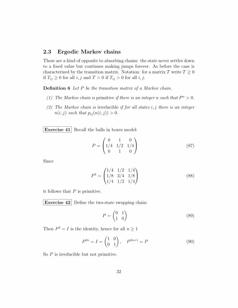
2.3 Ergodic Markov chains
These are a kind of opposite to absorbing chains: the state never settles downto a fixed value but continues making jumps forever. As before the case ischaracterized by the transition matrix. Notation: for a matrix T write T ≥ 0if Tij ≥ 0 for all i, j and T > 0 if Tij > 0 for all i, j.
Definition 6 Let P be the transition matrix of a Markov chain.
(1) The Markov chain is primitive if there is an integer n such that P n > 0.
(2) The Markov chain is irreducible if for all states i, j there is an integern(i, j) such that pij(n(i, j)) > 0.
Exercise 41 Recall the balls in boxes model:
P =
0 1 01/4 1/2 1/40 1 0
(87)
Since
P 2 =
1/4 1/2 1/41/8 3/4 1/81/4 1/2 1/4
(88)
it follows that P is primitive.
Exercise 42 Define the two-state swapping chain:
P =
(0 11 0
)(89)
Then P 2 = I is the identity, hence for all n ≥ 1
P 2n = I =
(1 00 1
), P 2n+1 = P (90)
So P is irreducible but not primitive.
32

Let e denote the vector in Rn with all entries 1, so
e =
11...1
(91)
Theorem 7 [Perron-Frobenius] Suppose P is a primitive n × n transitionmatrix. Then there is a unique strictly positive vector w ∈ Rn such that
wTP = wT (92)
and such that
P k → ewT as k →∞ (93)
Proof: we show that for all vectors y ∈ Rn,
P ky → ewTy (94)
which is a positive multiple of the constant vector e. This implies the result.Suppose first that P > 0 so that pij > 0 for all i, j ∈ S. Let d > 0 be the
smallest entry in P (so d ≤ 1/2). For any y ∈ Rn define
m0 = minj
yj, M0 = maxj
yj (95)
and
m1 = minj
(Py)j, M1 = maxj
(Py)j (96)
Consider (Py)i =∑
j pijyj. This is maximized by pairing the smallest entrym0 of y with the smallest entry d of pij, and then taking all other entries ofy to be M0. In other words,
M1 = maxi
(Py)i
= maxi
∑j
pijyj
≤ (1− d)M0 + dm0 (97)
33

By similar reasoning,
m1 = mini
(Py)i ≥ (1− d)m0 + dM0 (98)
Subtracting these bounds gives
M1 −m1 ≤ (1− 2d)(M0 −m0) (99)
Now we iterate to give
Mk −mk ≤ (1− 2d)k (M0 −m0) (100)
where again
Mk = maxi
(P ky)i, mk = mini
(P ky)i (101)
Furthermore the sequence Mk is decreasing since
Mk+1 = maxi
(PP ky)i = maxi
∑j
pij(Pky)j ≤Mk (102)
and the sequence mk is increasing for similar reasons. Therefore both se-quences converge as k →∞, and the difference between them also convergesto zero. Hence we conclude that the components of the vector P ky convergeto a constant value, meaning that
P ky → me (103)
for some m. We can pick out the value of m with the inner product
m(eT e) = eT limk→∞
P ky = limk→∞
eT P ky (104)
Note that for k ≥ 1,
eT P ky ≥ mk(eT e) ≥ m1(e
T e) = mini
(Py)i(eT e)
Since P is assumed positive, if yi ≥ 0 for all i it follows that (Py)i > 0 forall i, and hence m > 0.
Now define
wj = limk→∞
P kej/(eT e) (105)
34

where ej is the vector with entry 1 in the jth component, and zero elsewhere.It follows that wj > 0 so w is strictly positive, and
P k → ewT (106)
By continuity this implies
limk→∞
P kP = ewTP (107)
and hence wTP = wT . This proves the result in the case where P > 0.
Now turn to the case where P is primitive. Since P is primitive, thereexists integer N such that
PN > 0 (108)
Hence by the previous result there is a strictly positive w ∈ Rn such that
P kN → ewT (109)
as k → ∞, satisfying wTPN = wT . It follows that PN+1 > 0, and hencethere is also a vector v such that
P k(N+1) → evT (110)
as k → ∞, and vTPN+1 = vT . Considering convergence along the subse-quence kN(N + 1) it follows that w = v, and hence
wTPN+1 = vTPN+1 = vT = wT = wTPN (111)
and so
wTP = wT (112)
The subsequence P kNy converges to ewTy for every y, and we want to showthat the full sequence Pmy does the same. For any ε > 0 there is K < ∞such that for all k ≥ K and all probability vectors y
‖(P kN − ewT )y‖ ≤ ε (113)
Let m = kN + j where j < N , then for any probability vector y
‖(Pm − ewT )y‖ = ‖(P kN+j − ewT )y‖ = ‖(P kN − ewT )P jy‖ ≤ ε (114)
35

which proves convergence along the full sequence.
QED
Note that as a corollary of the Theorem we deduce that the vector w isthe unique (up to scalar multiples) solution of the equation
wTP = wT (115)
Also since vT e =∑vi = 1 for a probability vector v, it follows that
vTP n → wT (116)
for any probability vector v.
Exercise 43 Recall the balls in boxes model:
P =
0 1 01/4 1/2 1/40 1 0
(117)
We saw that P is primitive. Solving the equation wTP = wT yields thesolution
wT = (1/6, 2/3, 1/6) (118)
Furthermore we can compute
P 10 =
0.167 0.666 0.1670.1665 0.667 0.16650.167 0.666 0.167
(119)
showing the rate of convergence.
Aside on convergence [Seneta]: another way to express the Perron-Frobeniusresult is to say that for the matrix P , 1 is the largest eigenvalue (in absolutevalue) and w is the unique eigenvector (up to scalar multiples). Let λ2 bethe second largest eigenvalue of P so that 1 > |λ2| ≥ |λi|. Let m2 be themultiplicity of λ2. Then the following estimate holds: there is C < ∞ suchthat for all n ≥ 1
‖P n − ewT‖ ≤ C nm2−1 |λ2|n (120)
36

So the convergence P n → ewT is exponential with rate determined by thefirst spectral gap.
Concerning the interpretation of the result. Suppose that the distributionof X0 is
P (X0 = i) = αi (121)
for all i ∈ S. Then
P (Xk = j) =∑i
P (Xk = j|X0 = i)P (X0 = i) =∑i
(P k)ij αi = (αTP k)j(122)
where α is the vector with entries αi. Using our Theorem we deduce that
P (Xk = j)→ wj (123)
as k →∞ for any initial distribution α. Furthermore if α = w then αTP k =wTP k = wT and therefore
P (Xk = j) = wj (124)
for all k. So w is called the equilibrium or stationary distribution of thechain. The Theorem says that the state of the chain rapidly forgets itsinitial distribution and converges to the stationary value.
Now suppose the chain is irreducible but not primitive. Then we get asimilar but weaker result.
Theorem 8 Let P be the transition matrix of an irreducible Markov chain.Then there is a unique strictly positive probability vector w such that
wTP = wT (125)
Furthermore
1
n+ 1
(I + P + P 2 + · · ·+ P n
)→ ewT (126)
as n→∞.
37

Proof: define
Q =1
2I +
1
2P (127)
Then Q is a transition matrix. Also
2nQn =n∑k=0
(nk
)P k (128)
Because the chain is irreducible, for all pairs of states i, j there is an integern(i, j) such that (P n(i,j))ij > 0. Let n = maxn(i, j), then for all i, j we have
2n(Qn)ij =n∑k=0
(nk
)(P k)ij ≥
(n
n(i, j)
)(P n(i,j))ij > 0 (129)
and hence Q is primitive. Let w be the unique stationary vector for Q then
wTQ = wT ↔ wTP = wT (130)
which shows existence and uniqueness for P .Let W = ewT then a calculation shows that for all n(
I + P + P 2 + · · ·+ P n−1)
(I − P +W ) = I − P n + nW (131)
Note that I − P +W is invertible: indeed if yT (I − P +W ) = 0 then
yT − yTP + (yT e)w = 0 (132)
Multiply by e on the right and use Pe = e to deduce
yT e− yTPe+ (yT e)(wT e) = (yT e)(wT e) = 0 (133)
Since wT e = 1 > 0 it follows that yT e = 0 and so yT − yTP = 0. Byuniqueness this means that y is a multiple of w, but then yT e = 0 meansthat y = 0. Therefore I − P +W is invertible, and so
I + P + P 2 + · · ·+ P n−1 = (I − P n + nW )(I − P +W )−1 (134)
Now WP = W = W 2 hence
W (I − P +W ) = W =⇒ W = W (I − P +W )−1 (135)
38
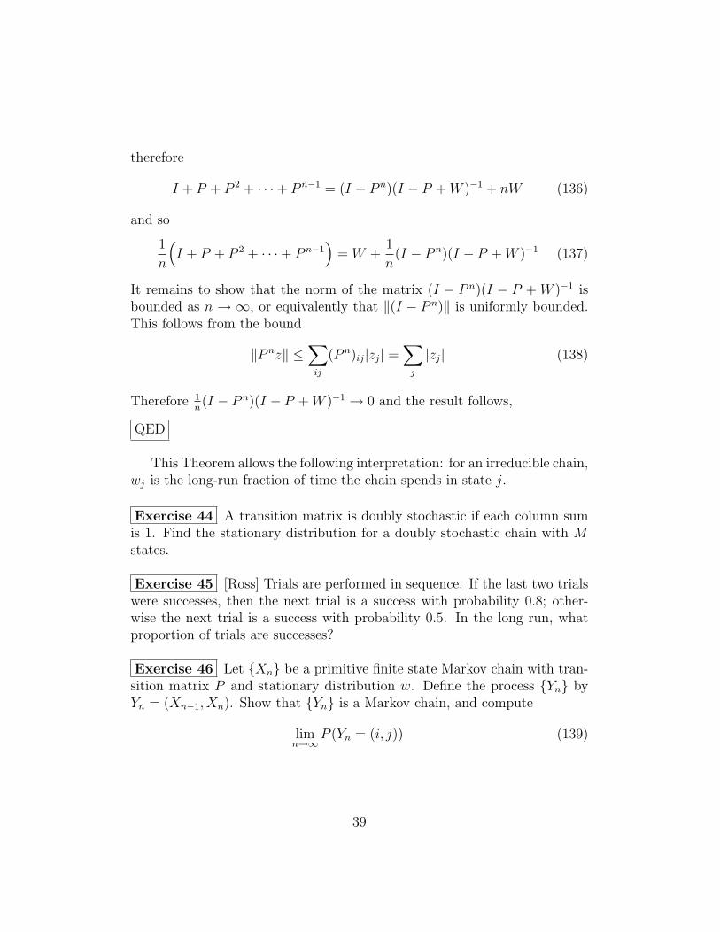
therefore
I + P + P 2 + · · ·+ P n−1 = (I − P n)(I − P +W )−1 + nW (136)
and so
1
n
(I + P + P 2 + · · ·+ P n−1
)= W +
1
n(I − P n)(I − P +W )−1 (137)
It remains to show that the norm of the matrix (I − P n)(I − P + W )−1 isbounded as n → ∞, or equivalently that ‖(I − P n)‖ is uniformly bounded.This follows from the bound
‖P nz‖ ≤∑ij
(P n)ij|zj| =∑j
|zj| (138)
Therefore 1n(I − P n)(I − P +W )−1 → 0 and the result follows,
QED
This Theorem allows the following interpretation: for an irreducible chain,wj is the long-run fraction of time the chain spends in state j.
Exercise 44 A transition matrix is doubly stochastic if each column sumis 1. Find the stationary distribution for a doubly stochastic chain with Mstates.
Exercise 45 [Ross] Trials are performed in sequence. If the last two trialswere successes, then the next trial is a success with probability 0.8; other-wise the next trial is a success with probability 0.5. In the long run, whatproportion of trials are successes?
Exercise 46 Let Xn be a primitive finite state Markov chain with tran-sition matrix P and stationary distribution w. Define the process Yn byYn = (Xn−1, Xn). Show that Yn is a Markov chain, and compute
limn→∞
P (Yn = (i, j)) (139)
39

Definition 9 Consider an irreducible Markov chain.
(1) starting in state i, mij is the expected number of steps to visit state jfor the first time (by convention mii = 0)
(2) starting in state i, ri is the expected number of steps for the first returnto state i
(3) the fundamental matrix is Z = (I − P +W )−1
Theorem 10 Let w be the stationary distribution of an irreducible Markovchain. Then for all states i, j ∈ S,
ri =1
wi, mij =
zjj − zijwj
(140)
where zij is the (i, j) entry of the fundamental matrix Z.
Proof: let M be the matrix with entries Mij = mij, let E be the matrixwith entries Eij = 1, and let D be the diagonal matrix with diagonal entriesDii = ri. For all i 6= j,
mij = pij +∑k 6=j
pik(mkj + 1) = 1 +∑k 6=j
pikmkj (141)
For all i,
ri =∑k
pik(mki + 1) = 1 +∑k
pikmki (142)
Thus for all i, j,
Mij = 1 +∑k 6=j
pikMkj −Dij (143)
which can be written as the matrix equation
M = E + PM −D (144)
Multiplying on the left by wT and noting that wT = wTP gives
0 = wTE − wTD (145)
40

The ith component of the right side is 1−wiri, hence this implies that for alli
ri =1
wi(146)
Recall the definition of the matrix Z = (I − P + W )−1, and vector e =(1, 1, . . . , 1)T . Since Pe = We = e it follows that (I − P + W )e = e andhence Ze = e and ZE = E = eeT . Furthermore wTP = wTW = wT and sosimilarly wTZ = wT and W = WZ. Therefore from (144),
Z(I − P )M = ZE − ZD = E − ZD (147)
Since Z(I − P ) = I − ZW = I −W this yields
M = E − ZD +WM (148)
The (i, j) component of this equation is
mij = 1− zijrj + (wTM)j (149)
Setting i = j gives 0 = 1− zjjrj + (wTM)j, hence
mij = (zjj − zij)rj =zjj − zijwj
(150)
QED
2.4 Classification of finite-state Markov chains
Say that states i and j intercommunicate if there are integers n,m such thatpij(n) > 0 and pji(m) > 0. In other words it is possible to go from each stateto the other. A class of states C in S is called closed if pij = 0 whenever i ∈ Cand j /∈ C. The class is called irreducible if all states in C intercommunicate.
Note that if the chain is irreducible then all states intercommunicate andhence for all i, j there is an integer n such that pij(n) > 0.
Theorem 11 The state space S can be partitioned uniquely as
S = T ∪ C1 ∪ C2 ∪ · · · (151)
where T is the set of all transient states, and each class Ci is closed andirreducible.
41

Proof: (later)If the chain starts with X0 ∈ Ci then it stays in Ci forever. If it starts
with X0 ∈ T then eventually it enters one of the classes Ci and stays thereforever.
Exercise 47 Determine the classes of the chain:
P =
1/2 1/2 0 0 0 01/4 3/4 0 0 0 01/4 1/4 1/4 1/4 0 01/4 0 1/4 1/4 0 1/40 0 0 0 1/2 1/20 0 0 0 1/2 1/2
(152)
42

3 Existence of Markov Chains
We have been making an implicit assumption about the Markov chains, andnow it is time to address this openly. Namely, we have been assuming thatthe statement “letX0, X1, . . . be random variables . . . ” makes sense. Becausewe use the joint distribution for the Xi we need to know that they all existas random variables on the same underlying sample space, with the sameunderlying probability function. If we use a finite number of Xi then there isno problem, we are still working with simple random variables. But we wantto consider an infinite number at the same time: for example what does itmean to say (as we did) “ limn→∞ P (Xn = j) ”? To make sense of this atthe very least we need all Xn to be defined as random variables on the samesample space. So let’s do that. We will handle the case of a countable statespace at the same time.
3.1 Sample space for Markov chain
Let S be the countable state space of a Markov chain. Let αi and pij berespectively the initial distribution of X0 and the transition matrix of thechain. This means that
P (X0 = i) = αi for all i ∈ S (153)
and also that
P (Xn+1 = j |Xn = i) = pij for all i, j ∈ S, all n ≥ 1 (154)
The joint distribution of the Xi follows from this: for example
P (X2 = k,X1 = j,X0 = i) = P (X2 = k |X1 = j)P (X1 = j |X0 = i)P (X0 = i)
= pjk pij αi
In general we have
P (X0 = i0, X1 = i1, . . . , Xn = in) = αi0 pi0i1 . . . pin−1in (155)
We want a sample space Ω with a probability function P defined on it sothat for all n
Xn : Ω→ S (156)
43

and so that the joint pmf is given as above.
We take Ω = [0, 1], that is the closed interval of real numbers. We takethe probability function P to be the ‘usual’ length function (more aboutthis shortly). So an event in Ω is a subset of [0, 1], say A ⊂ [0, 1], and theprobability of A is the ‘length’ of A. For example if A = (a, b] then
P (A) = length(a, b] = |b− a| (157)
Of course we need to extend the notion of length to more general subsets.But assuming that there is such an extension then we define the randomvariables as follows.
a) Partition [0, 1] into S subintervals, call them
I(0)i i ∈ S
with length(I(0)i ) = αi for each i. Since
∑i αi = 1 this covers the whole
interval.
b) Partition each such interval I(0)i into further subintervals
I(1)i,j j∈S
so that for every i, j ∈ S we have length(I(1)i,j ) = αi pij. Again note that∑
j pij = 1 so we are covering the whole interval I(0)i .
c) Inductively partition [0, 1] into intervals I(n)i0,i1,...,in
such that they are
nested according to I(n)i0,i1,...,in
⊂ I(n−1)i0,i1,...,in−1
, and so that their lengths are
given by length(I(n)i0,i1,...,in
) = αi0 pi0i1 . . . pin−1in .
d) Define Xn by Xn(x) = in if x ∈ I(n)i0,i1,...,in
for some choice of i0, i1, . . . , in−1.
It remains to verify that Xn have the required joint distribution. Firstnote that
P (X0 = i) = P (x ∈ I(0)i ) = length I
(0)i = αi (158)
Then note that
P (X1 = j,X0 = i) = P (x ∈ I(1)i,j ) = length I
(1)i,j = pij αi (159)
The general case follows just as easily.
To summarize: we have exhibited the random variables X0, X1, . . . asfunctions on the same probability space namely Ω = [0, 1], equipped withthe probability function defined by the usual length.
44

3.2 Lebesgue measure
To complete the demonstration we need to extend the notion of length toinclude more general subsets of [0, 1]. Why is this? Suppose we want tocalculate
P (Xn = i infinitely often)
This event can be written as
Xn = i infinitely often =∞⋃n=1
∞⋂k=n
Xk = i (160)
On the right side we have an infinite union of an infinite intersection ofintervals. What is the length of such a set? Clearly we need to extend thenotion of length.
The correct extension is called the Lebesgue measure, or just the measure.We will delve into this shortly but here we just note that it is possible to doit in such a way that we can consistently assign a probability to the rightside above, and in fact make sense of any such complicated event that mightarise in the study of our Markov chains.
45

4 Discrete-time Markov chains with count-
able state space
Moving from a finite state space to an infinite but countable state space leadsto novel effects and a broader class of applications. The basic setup is thesame as before: a finite or countably infinite state space S, a sequence of S-valued random variables X0, X1, . . . , and a set of transition probabilitiespij for each pair of states i, j ∈ S. The Markov property is the same:
P (Xn = y |X0 = x0, . . . , Xn−1 = xn−1) = P (Xn = y |Xn−1 = xn−1) (161)
for all n ≥ 1 and all states y, x0, . . . , xn−1 ∈ S. Also the transition ‘matrix’satisfies ∑
j∈S
pij = 1 for all i ∈ S (162)
4.1 Some motivating examples
The one-dimensional random walk has state space Z = . . . ,−1, 0, 1, . . . ,and transition probabilities
pij =
p if j = i+ 1
q if j = i− 1
0 else
(163)
So at each time unit the chain takes one step either to the left or the right,with probabilities q and p respectively. The chain has no absorbing statesso it keeps moving forever. Interesting questions are whether it wanders offto infinity or stays around its starting position, and also rates of variouslong-run behavior.
A second important example is the branching process. This describes thegrowth of a population. The state is the number of individuals in succes-sive generations. This changes because of the random number of births anddeaths. In the simplest case each individual produces a random number ofindividuals B in the next generation:
Xn+1 =Xn∑i=1
Bi
46

There is one absorbing state corresponding to extinction. So the interestingquestion is whether the chain reaches extinction or keeps growing forever –or more precisely, the probability that it ever reaches extinction.
4.2 Classification of states
Define
fij(n) = P (X1 6= j,X2 6= j, . . . , Xn−1 6= j,Xn = j |X0 = i) (164)
to be the probability that starting in state i the chain first visits state j aftern steps. Define
fij =∞∑n=1
fij(n) (165)
This is the probability that the chain eventually visits state j starting instate i.
Definition 12 The state j is persistent if fjj = 1. The state j is transientif fjj < 1.
There is a further separation of persistent states which occurs for infinitestate space.
Definition 13 The mean return time µj of state j is
µj =
∑∞n=1 nfjj(n) if j is persistent
∞ if j is transient(166)
Note that µj may be finite or infinite for a persistent state (this is what wecalled rj for the finite state space).
Definition 14 The persistent state j is null-persistent if µj =∞, and it isnon-null persistent if µj <∞.
So there are three types of states in a Markov chain: transient, nullpersistent and non-null persistent. This is the classification of states.
47

Exercise 48 Define generating functions
Pij(s) =∞∑n=0
snpij(n), Fij(s) =∞∑n=0
snfij(n) (167)
with the conventions pij(0) = δij and fij(0) = 0. Show that
Pii(s) = 1 + Fii(s)Pii(s) (168)
Show that state i is persistent if and only if∑
n pii(n) =∞.[Hint: recall Abel’s theorem: if an ≥ 0 for all n and
∑n ans
n is finite for all|s| < 1, then
lims↑1
∞∑n=0
ansn =
∞∑n=0
an (169)
4.3 Classification of Markov chains
Say that states i and j intercommunicate if there are integers n,m such thatpij(n) > 0 and pji(m) > 0. In other words it is possible to go from each stateto the other.
Theorem 15 Let i, j intercommunicate, then they are either both transient,both null persistent or both non-null persistent.
Proof: Since i, j intercommunicate there are integers n,m such that
h = pij(n)pji(m) > 0 (170)
Hence for any r,
pii(n+m+ r) ≥ pij(n)pjj(r)pji(m) = h pjj(r) (171)
Sum over r to deduce∑k
pii(k) ≥∑r
pii(n+m+ r) ≥ h∑r
pjj(r) (172)
48

Therefore either both sums are finite or both are infinite, hence either bothstates are transient or both are persistent. [Omit the proof about null per-sistent and non-null persistent].
QED
Exercise 49 Suppose that state i is transient, and that state i is accessiblefrom state j. Show that pij(n)→ 0 as n→∞.
A class of states C in S is called closed if pij = 0 whenever i ∈ C andj /∈ C. The class is called irreducible if all states in C intercommunicate.
This usage is consistent with the finite state space case – if the chain isan irreducible class then all states intercommunicate and hence for all i, jthere is an integer n such that pij(n) > 0.
Theorem 16 The state space S can be partitioned uniquely as
S = T ∪ C1 ∪ C2 ∪ · · · (173)
where T is the set of all transient states. Each class Ci is closed and ir-reducible, and contains persistent states. Either all states in Ci are nullpersistent, or all states in Ci are non-null persistent.
Proof: mostly clear except maybe that Ci is closed. So suppose indeed thatthere are states i ∈ C and j /∈ C with pij > 0. Since i is not accessible fromj, it follows that pji(n) = 0 for all n ≥ 1. Hence
1− fii = P (Xn 6= i for all n ≥ 1|X0 = i) ≥ P (X1 = j|X0 = i) = pij (174)
which means that fii < 1, but this contradicts the persistence of state i.
QED
If the chain starts with X0 ∈ Ci then it stays in Ci forever. If it startswith X0 ∈ T then eventually it enters one of the classes Ci and stays thereforever. We will restrict attention to irreducible chains now. The first issueis to determine which of the three types of chains it may be. Recall the
49

definition of a stationary distribution of the chain: this is a distribution πsuch that πi ≥ 0 and
∑i πi = 1, and for all j ∈ S,
πj =∑i
πi pij (175)
(it is conventional to use π for discrete chains, we do so from now on).
Theorem 17 Consider an irreducible chain with transition probabilities pij.
(1) The chain is transient if and only if∑
n pjj(n) <∞ for any (and henceall) states j ∈ S.
(2) The chain is persistent if and only if∑
n pjj(n) = ∞ for any (andhence all) states j ∈ S.
(3) There is a positive vector x satisfying xT = xTP , that is
xj =∑i∈S
xipij (176)
The chain is non-null persistent if and only if∑
i xi <∞.
(4) If the chain has a stationary distribution then it is non-null persistent.
In case (3) we can normalize x by dividing by∑
i xi and hence recoverthe stationary distribution π. Thus as a Corollary we see that a chain has astationary distribution if and only if it is non-null persistent.Proof: items (1), (2) were shown in the exercises. For item (4), suppose thatπ is a stationary distribution and note that if the chain is transient thenpij(n)→ 0 for all states i, j and hence
πj =∑i
πipij(n)→ 0 (177)
(this needs a little care when the sum is infinite – see Comment after theproof of Theorem 20).
Turn to item (3). Fix a state k, and let Tk be the time (number of steps)until the first return to state k. Let Ni(k) be the time spent in state i duringthis sojourn, or more precisely,
Ni(k) =∞∑n=1
1Xn=i∩Tk≥n (178)
50

It follows that Nk(k) = 1. Hence
Tk =∑i∈S
Ni(k) (179)
By definition
µk = E[Tk |X0 = k] (180)
Define ρi(k) = E[Ni(k) |X0 = k] then
µk =∑i∈S
ρi(k) (181)
It turns out that ρi(k) will yield the components of the stationary distribu-tion.
First we claim that ρi(k) <∞. To see this, write
Lki(n) = E[1Xn=i∩Tk≥n] = P (Xn = i ∩ Tk ≥ n) (182)
so that E[Ni(k)] =∑∞
n=1 Lki(n). Now
fkk(m+ n) ≥ Lki(n) fik(m) (183)
Choose m so that fik(m) > 0 (chain is irreducible) then
Lki(n) ≤ fkk(m+ n)
fik(m)(184)
Hence
ρi(k) = E[Ni(k) |X0 = k]
=∞∑n=1
Lki(n)
≤∞∑n=1
fkk(m+ n)
fik(m)
≤ 1
fik(m)<∞ (185)
51

Next we claim that ρi is stationary. Note that for n ≥ 2,
Lki(n) =∑j 6=k
Lkj(n− 1)pji (186)
Hence
ρi(k) = Lki(1) +∞∑n=2
Lki(n)
= pki +∑j 6=k
∞∑n=2
Lkj(n− 1)pji
= pki +∑j 6=k
ρj(k)pji
=∑j∈S
ρj(k)pji (187)
where in the last equality we used ρk(k) = 1 (true because Nk(k) = 1). Henceρi(k) is stationary.
So for every k ∈ S we have a stationary vector. The chain is non-nullpersistent if and only if µk < ∞, in which case we can normalize to get aprobability distribution. It remains to show that this distribution is uniqueand positive. For positivity, suppose that πj = 0 for some j, then
0 =∑i
πipij(n) ≥ πipij(n) (188)
for all i and n. Hence if i and j communicate then πi = 0 also. But the chainis irreducible, hence πi = 0 for all i ∈ S. For uniqueness, use the followingTheorem 20.
QED
Definition 18 The state i is aperiodic if
1 = gcdn | pii(n) > 0 (189)
If a chain is irreducible then either all states are aperiodic or none are.
Exercise 50 Construct the coupled chain Z = (X, Y ) consisting of theordered pair of independent chains with the same transition matrix P . If
52

X and Y are irreducible and aperiodic, show that Z is also irreducible andaperiodic. [Hint: use the following theorem: “An infinite set of integers whichis closed under addition contains all but a finite number of positive multiplesof its greatest common divisor” [Seneta]].
Definition 19 An irreducible, aperiodic, non-null persistent Markov chainis called ergodic.
Theorem 20 For an ergodic chain,
pij(n)→ πj =1
µj(190)
as n→∞, for all i, j ∈ S.
Proof: Use the coupled chain described above. It follows that Z is alsoergodic. Suppose that X0 = i and Y0 = j, so Z0 = (i, j). Choose s ∈ S anddefine
T = minn ≥ 1 |Zn = (s, s) (191)
This is the ‘first passage time’ to state (s, s). Hence
pik(n) = P (Xn = k)
= P (Xn = k, T ≤ n) + P (Xn = k, T > n)
= P (Yn = k, T ≤ n) + P (Xn = k, T > n)
≤ P (Yn = k) + P (T > n)
= pjk(n) + P (T > n) (192)
where we used the fact that if T ≤ n then Xn and Yn have the same distri-bution. This and related inequality with i and j switched gives
|pik(n)− pjk(n)| ≤ P (T > n) (193)
But since Z is persistent, P (T <∞) = 1 and hence
|pik(n)− pjk(n)| → 0 (194)
53

as n→∞. Furthermore, let π be a stationary distribution for X, then
πk − pjk(n) =∑i
πi (pik(n)− pjk(n))→ 0 (195)
as n→∞. Together (194) and (195) show that pjk(n) converges as n→∞ toa limit which does not depend on j or on the choice of stationary distributionfor X. Hence there is a unique stationary distribution for X. Finally fromthe previous Theorem we had ρk(k) = 1 and so
πk =ρk(k)∑j ρj(k)
=1
µk(196)
QED
Comment: the limit in (195) needs to be justified. Let F be a finite subsetof S then∑
i
πi |pik(n)− pjk(n)| ≤∑i∈F
πi |pik(n)− pjk(n)|+ 2∑i/∈F
πi
→ 2∑i/∈F
πi (197)
as n→∞. Now take an increasing sequence of finite subsets Fa convergingto S, and use
∑i∈S πi = 1 to conclude that
∑i/∈Fa πi → 0.
Exercise 51 Show that the one-dimensional random walk is transient ifp 6= 1/2. If p = 1/2 (called the symmetric random walk) show that the chainis null persistent. [Hint: use Stirling’s formula for the asymptotics of n!:
n! ∼ nn e−n√
2πn (198)
Exercise 52 Consider a Markov chain on the set S = 0, 1, 2, . . . withtransition probabilities
pi,i+1 = ai, pi,0 = 1− ai
54

for i ≥ 0, where ai | i ≥ 0 is a sequence of constants which satisfy 0 < ai < 1for all i. Let b0 = 1, bi = a0a1 · · · ai−1 for i ≥ 1. Show that the chain is
(a) persistent if and only if bi → 0 as i→∞(b) non-null persistent if and only if
∑i bi <∞,
and write down the stationary distribution if the latter condition holds.
Let A and β be positive constants and suppose that ai = 1−Ai−β for alllarge values of i. Show that the chain is
(c) transient if β > 1(d) non-null persistent if β < 1. Finally, if β = 1 show that the chain is
(e) non-null persistent if A > 1(f) null persistent if A ≤ 1.
Exercise 53 For a branching process the population after n steps can bewritten as
Xn =
Xn−1∑i=1
Zi (199)
where X0 = 1, and where Zi is the number of offspring of the ith individualof the (n − 1)st generation. It is assumed that all the variables Zi are IID.Let π0 be the probability that the population dies out,
π0 = limn→∞
P (Xn = 0 |X0 = 1) (200)
Show that π0 is the smallest positive number satisfying the equation
π0 =∞∑j=0
πj0 P (Z = j) (201)
[Hint: define the generating functions φ(s) = EsZ and φn(s) = EsXn fors > 0. Show that φn+1(s) = φ(φn(s)) and deduce that π0 is a fixed point ofφ.]
55
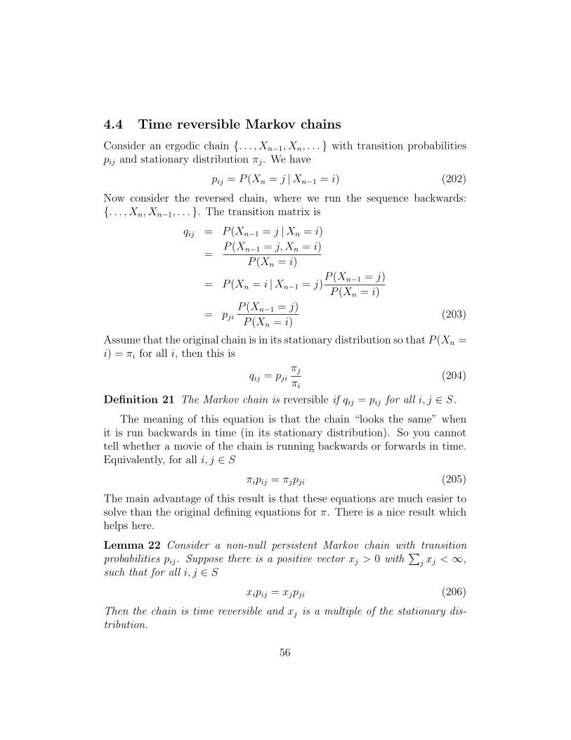
4.4 Time reversible Markov chains
Consider an ergodic chain . . . , Xn−1, Xn, . . . with transition probabilitiespij and stationary distribution πj. We have
pij = P (Xn = j |Xn−1 = i) (202)
Now consider the reversed chain, where we run the sequence backwards:. . . , Xn, Xn−1, . . . . The transition matrix is
qij = P (Xn−1 = j |Xn = i)
=P (Xn−1 = j,Xn = i)
P (Xn = i)
= P (Xn = i |Xn−1 = j)P (Xn−1 = j)
P (Xn = i)
= pjiP (Xn−1 = j)
P (Xn = i)(203)
Assume that the original chain is in its stationary distribution so that P (Xn =i) = πi for all i, then this is
qij = pjiπjπi
(204)
Definition 21 The Markov chain is reversible if qij = pij for all i, j ∈ S.
The meaning of this equation is that the chain “looks the same” whenit is run backwards in time (in its stationary distribution). So you cannottell whether a movie of the chain is running backwards or forwards in time.Equivalently, for all i, j ∈ S
πipij = πjpji (205)
The main advantage of this result is that these equations are much easier tosolve than the original defining equations for π. There is a nice result whichhelps here.
Lemma 22 Consider a non-null persistent Markov chain with transitionprobabilities pij. Suppose there is a positive vector xj > 0 with
∑j xj < ∞,
such that for all i, j ∈ S
xipij = xjpji (206)
Then the chain is time reversible and xj is a multiple of the stationary dis-tribution.
56

So this result says that if you can find a positive solution of the simplerequation then you have solved for the stationary distribution.
Exercise 54 A total of m white and m black balls are distributed amongtwo boxes, with m balls in each box. At each step, a ball is randomly selectedfro each box and the two selected balls are exchanged and put back in theboxes. Let Xn be the number of white balls in the first box. Show that thechain is time reversible and find the stationary distribution.
The quantity πipij has another interpretation: it is the rate of jumps ofthe chain from state i to state j. More precisely, it is the long-run averagerate at which the chain makes the transition between these states:
limn→∞
P (Xn = i , Xn+1 = j) = πipij (207)
This often helps to figure out if a chain is reversible.
Exercise 55 Argue that any Markov chain on Z which makes jumps onlybetween nearest neighbor sites is reversible.
Exercise 56 Consider a Markov chain on a finite graph. The states are thevertices, and jumps are made along edges connecting vertices. If the chain isat a vertex with n edges, then at the next step it jumps along an edge withprobability 1/n. Argue that the chain is reversible, and find the stationarydistribution.
57

5 Probability triples
5.1 Rules of the road
Why do we need to go beyond elementary probability theory? We alreadysaw the need even for finite state Markov chains. Here is an analogy. Whenyou drive along the road you operate under the assumption that the road willcontinue after the next bend (even though you cannot see it before gettingthere). So you can rely on an existence theorem, namely that the road systemof the country is constructed in such a way that roads do not simply ‘end’without warning, and that you will not drive over a cliff if you follow theroad. Another way of saying this is that you trust that by following the rulesof the road you can proceed toward your destination. Of course whether youreach your destination may depend on your map-reading ability and skill infollowing directions, but that is another matter!
So let’s apply this analogy to probability theory. Our ‘rules of the road’are the basic definitions and operations introduced before, including events,probabilities, random variables and so on. Our destination may be quitecomplicated, for example: “what is the probability that the pattern HHT-THH will appear infinitely often if a coin is repeatedly tossed?”. In order toanswer this question we will take our simple rules and push them beyond thelimits of elementary probability. So we will not be able to use mental models(imagine tossing infinitely many coins!) or rely on our intuition about whatis or is not reasonable. We want to know that our methods will make senseout there, and that there will be a sample space and an event for which wecan compute this probability. We don’t want to ‘fall off a cliff’ and end upproving that 0 = 1! So we need an existence theorem that gives conditions(‘rules of the road’) which will guarantee that we will not end up with math-ematical nonsense. This is the business addressed in this section. It turnsout to be difficult because there really are dangerous cliffs out there.
5.2 Uncountable sample spaces
We resolved the Markov chain existence question by pushing it onto theproblem of defining a measure on the interval [0, 1]. The resolution is ageneral theory that applies to any probability model. So we introduce thegeneral theory first and then apply it to the Lebesgue measure. As a bonuswe will see how to define continuous random variables also.
58

For uncountable sample spaces a new kind of difficulty arises when tryingto define a probability law. We want to maintain the consistency relations asbefore, in particular countable additivity: if E1, E2, . . . , En, . . . is a sequenceof pairwise disjoint events, then we want
P (∞⋃n=1
En) =∞∑n=1
P (En) (208)
But there are so many subsets of an infinite sample space S that it turnsout to be impossible to satisfy countable additivity for all sequences of disjointsets. Something has to give. The resolution is to restrict the class of eventsby excluding some subsets of S. The class of events should still be largeenough to include everything we encounter in practice, and it should alsoinclude everything we can get by combining events in the usual way. Thecorrect formulation is called a σ-algebra.
5.3 σ-algebras
Definition 23 Let S be a nonempty set. A σ-algebra in S is a collection ofsubsets A satisfying the following conditions:
(1) S ∈ A
(2) if A ∈ A then Ac ∈ A
(3) if A1, A2, . . . is a countable collection of sets in A, then their union⋃nAn also belongs to A
These properties are expressed by saying A is closed under complementsand countable unions.
Exercise 57 Show that A is also closed under countable intersections.
We summarize this by saying that A is closed under the operations ofcomplement, countable union and countable intersection. Note however thatin general an uncountable union or intersection of sets in A will not be con-tained in A. For this reason there may be subsets of S which are not in thecollection A.
Clearly the collection of all subsets of S is a σ-algebra.
59

Exercise 58 Let A be the subsets of S which are either countable or whosecomplement is countable. Show that A is a σ-algebra.
So in our new way of thinking a sample space S will be equipped witha σ-algebra A, and only the sets in A will be considered as events. So theprobability law needs to be defined only on A.
Definition 24 A probability triple (S,A, P ) consists of a nonempty set S, aσ-algebra A in S, and a map P : A → [0, 1] satisfying(i) 0 ≤ P (A) for all A ∈ A,(ii) P (S) = 1,(iii) if A1, A2, . . . is a pairwise disjoint sequence of sets in A then
P (∞⋃n=1
An) =∞∑n=1
P (An) (209)
The axioms given are tightly compressed, and imply a host of other re-lations. For example, a finite sequence A1, . . . , An can be augmented toA1, . . . , An, ∅, . . . and then (iii) provides finite additivity. Since A ∩ Ac = ∅and S = A ∪ Ac, it follows from (ii) and (iii) that
1 = P (S) = P (A) + P (Ac) (210)
This also implies monotonicity: if A ⊂ B then B = A∪ (B−A) is a disjointunion, so P (B) = P (A) + P (B − A) ≥ P (A).
Exercise 59 Derive the inclusion-exclusion formula:
P (n⋃k=1
Ak) =∑i
P (Ai)−∑i<j
P (Ai ∩ Aj)
+∑i<j<k
P (Ai ∩ Aj ∩ Ak) + · · ·+ (−1)n+1 P (A1 ∩ · · · ∩ An)(211)
There is one important special case, namely whereA = 2S is the σ-algebraof all subsets of S. When S is finite or countable and P is any map on Ssatisfying
∑s∈S p(s) = 1, then the probability triple can always be taken as
(S, 2S, P ), and in this case all subsets are events. But if S is uncountablethen it may not be possible to extend P to a map on the σ-algebra 2S.
60

The important thing to recognize is that we are putting conditions on(S,A, P ) by demanding that these properties are satisfied. As we will seethese conditions are enough to guarantee that we will ‘stay on the road’ ifwe follow the rules.
5.4 Continuity
The axioms guarantee that P has a nice continuity property. A sequenceAn of sets is increasing if An ⊂ An+1 for all n. The limit of this sequenceis defined to be
⋃∞n=1An. Similarly a sequence An is decreasing if Acn is
increasing, and the limit is then⋂∞n=1An.
Lemma 25 If An are increasing then P (An) is increasing and limP (An) =P (⋃∞n=1An). If An are decreasing then P (An) is decreasing and limP (An) =
P (⋂∞n=1An).
Proof: suppose An are increasing. For each n ≥ 1 define
Bn+1 = An+1 − An, B1 = A1 (212)
Then Bn are disjoint, and for every N ≥ 1
N⋃n=1
An =N⋃n=1
Bn (213)
as well as
∞⋃n=1
An =∞⋃n=1
Bn (214)
61

Hence
P (∞⋃n=1
An) = P (∞⋃n=1
Bn)
=∞∑n=1
P (Bn)
= limN→∞
N∑n=1
P (Bn)
= limN→∞
P (N⋃n=1
Bn)
= limN→∞
P (N⋃n=1
An)
= limN→∞
P (AN) (215)
QED
Exercise 60 Complete the proof for a decreasing sequence.
Recall that Exercise 5 derived countable subadditivity:
P (∞⋃n=1
An) ≤∞∑n=1
P (An) (216)
5.5 Draw breath
It is worth returning to the original reason for introducing σ-algebras, namelythe impossibility of satisfying the consistency relations (208) for all subsetsof S. At this point it is not clear that P can be defined even on the smallercollection of sets A. In fact this is possible, and leads to powerful models inprobability theory.
62

The issue of how to do this is tackled in probability theory by a generalstrategy. First there is a small class of sets where it is ‘obvious’ how to definethe probabilities. The probabilities defined on this small class are then usedto construct a function called outer measure that assigns a value P ∗(E) toevery subset E ⊂ S. The value P ∗(E) agrees with the original probabilityvalue on the small class of ‘obvious’ sets, but cannot be interpreted as aprobability for all sets. Finally a special σ-algebra A is identified where thefunction P ∗ satisfies the properties (i), (ii), (iii) required for a probabilitylaw. Then (S,A, P ∗) is the probability triple. When done in the right waythis leads to a sufficiently large σ-algebra that includes the events of interestfor the problem. Of course, once the probability law has been defined youcan start trying to compute probabilities of interesting events, which is wherethe real hard work starts!
A theory is only as good as its useful examples. We will shortly look athow Lebesgue measure is constructed. For the moment we note that property(iii) of the triple does not lead to inconsistencies.
Lemma 26 Suppose An and Bn are each pairwise disjoint sequences ofsets in A, and also
∞⋃n=1
An =∞⋃n=1
Bn (217)
Then
∞∑n=1
P (An) =∞∑n=1
P (Bn) (218)
Proof: Let E =⋃∞n=1An =
⋃∞n=1Bn. For all n,m define the set Cn,m =
An ∩Bm. Then the sets Cn,m are disjoint and belong to A, and
∞⋃n=1
Cn,m = E ∩Bm = Bm,
∞⋃m=1
Cn,m = An ∩ E = An (219)
63

Hence
∞∑n=1
P (An) =∞∑n=1
P (∞⋃m=1
Cn,m)
=∞∑n=1
∞∑m=1
P (Cn,m)
=∞∑m=1
∞∑n=1
P (Cn,m)
=∞∑m=1
P (∞⋃n=1
Cn,m)
=∞∑m=1
P (Bm) (220)
QED
So it follows that if a set A ∈ A can be decomposed in several differentways as a countable union of disjoint sets then the relation (iii) is satisfiedin every case. This is an important consistency check for the definition of aprobability law.
Exercise 61 Let A and B be σ-algebras in S. Show that A ∩ B is also aσ-algebra (note that C ∈ A ∩ B if and only if C ∈ A and C ∈ B).
5.6 σ-algebra generated by a class
For a finite collection of sets, you can enumerate all the sets obtained bytaking complements, unions and intersections of these sets. This larger col-lection is called the σ-algebra generated by the original set. This proceduredoes not work if you start with an infinite collection of sets, hence anothermethod of construction is needed.
Let C be a collection of subsets of S. Define σ(C) to be the smallest σ-algebra in S containing C. More precisely, C ⊂ σ(C) and if A is any σ-algebracontaining C then σ(C) ⊂ A. This is called the σ-algebra generated by C.The construction of σ(C) is quite strange but it gives a flavor of how thingsare done in the world of measure theory. First we note the following.
64

Lemma 27 Let T be a collection of σ-algebras, then B =⋂A∈T A is a σ-
algebra.
Proof: let Bk be a sequence in B, then Bk ∈ A for every A ∈ T , hence⋃Bk ∈ A for every A ∈ T , hence
⋃Bk ∈ B. Similarly B is closed under
complement.
QED
Now define T to be the collection of all σ-algebras in S which contain C.Then
σ(C) =⋂A∈T
A (221)
To see why this is true, note that⋂A∈T A is a σ-algebra, it contains C, and
it is the smallest σ-algebra which does so.
Exercise 62 Let C denote the collection of all half-open intervals (a, b] ⊂ Rwhere a < b. Show that σ(C) contains all intervals of the form (a, b), [a, b]and [a, b) with a < b.
5.7 Borel sets
The Borel sets constitute an important σ-algebra in R. They are built upby starting with the half-open intervals (a, b] where a < b. Let C be thecollection of all such intervals. Then the σ-algebra of Borel sets is defined tobe B = σ(C), that is the smallest σ-algebra containing all of these intervals.
The Borel σ-algebra B plays an important role because it is large enoughthat we can construct continuous random variables on (R,B, P ). Of coursewe have not specified P yet but there are plenty of ways to do this. For themoment we note some properties of B. Recall that we showed in Exercise 35that B contains all intervals of the form (a, b), [a, b] and [a, b) with a < b.
Exercise 63 Show that B contains all open and closed sets in R.[Hint: use the fact that every open set in R is a countable union of pairwisedisjoint open intervals].
65

In fact (though we will not prove it here) B is also the σ-algebra generatedby the open sets in R.
For the next exercise, recall that a function f : R → R is continuous ifand only if f−1(A) is open for every open set A ⊂ R.
Exercise 64 Let f : R→ R be continuous. Define
C = E ⊂ R : f−1(E) ∈ B (222)
Show that C is a σ-algebra. Show that C contains all open sets. Deduce thatB ⊂ C.
5.8 Lebesgue measure
This is the prototype for probability functions on continuous spaces. Thesubsets of R with an obvious length are the intervals:
l(a, b] = l(a, b) = |a− b| (223)
We want to extend this to a measure on the Borel sets. First define outermeasure for all subsets:
m∗(A) = inf ∞∑n=1
l(In) : A ⊂∞⋃n=1
In
(224)
where the infimum is taken over all countable collections of intervals whoseunion contains A. There is some work to do now. Must check that m∗(I) =l(I) for every interval, so that m∗ really is an extension of the length function.This is quite non-trivial, and requires using compactness properties of R.
The next step is to select a good collection of sets where countable addi-tivity will hold.
Definition 28 A set E ⊂ R is measurable if for every set A ⊂ R we have
m∗(A) = m∗(A ∩ E) +m∗(A ∩ Ec) (225)
So whenever a measurable set E divides a set A into two disjoint piecesA ∩ E and A ∩ Ec, the sum of the measures must equal the measure of thewhole. Let M be the collection of all measurable sets. The key result is thefollowing.
66

Lemma 29 M is a σ-algebra, and M contains the Borel sets. If En arepairwise disjoint sets in M, then
m∗(⋃
En) =∑
m∗(En) (226)
It follows that m∗ defines a measure onM, and this is called the Lebesguemeasure. Can check that it is translation invariant. The σ-algebra M isstrictly larger than the Borel sets B, but for most purposes the distinctionis irrelevant, and we restrict the measure to B. We will denote Lebesguemeasure by λ henceforth.
Exercise 65 Show Q has measure zero. Same for any countable set. Samefor the Cantor set.
Despite the complexity of their definition, the Borel sets are not too muchdifferent from open and closed sets, as the following result shows.
Lemma 30 Let B ∈ B be a Borel set. Then for every ε > 0, there is aclosed set F and an open set G such that F ⊂ B ⊂ G, and λ(B − F ) < εand λ(G−B) < ε.
Proof: first we construct the open set G which contains B. By definition ofouter measure, for every ε > 0 there is a countable union of open intervalsIn such that B ⊂
⋃In and
λ(B) = m∗(B) >∞∑n=1
l(In)− ε
Let G =⋃In, then G is open, B ⊂ G and
λ(G−B) = λ(G)− λ(B) ≤∞∑n=1
l(In)− λ(B) < ε
For the closed set inside F , take F c to be the open set containing Bc asabove.
QED
Exercise 66 Show that outer measure m∗ is translation invariant, that ism∗(A+ x) = m∗(A) for every A ⊂ R and every x ∈ R.
67

Exercise 67 Show that Lebesgue measure is complete: if B is measurableand λ(B) = 0, then every subset A ⊂ B is also measurable and λ(A) = 0.
5.9 Lebesgue-Stieltjes measure
The study of continuous random variables will lead us to a generalization ofLebesgue measure. Suppose that F : R → R is a non-decreasing functionwhich is continuous on the right. So if x < y then F (x) ≤ F (y), and for allx
F (x) = limh→0+
F (x+ h) (227)
Then we can assign a new measure to half-open intervals as follows:
µ(a, b] = F (b)− F (a) (228)
The construction of the Lebesgue measure can now be repeated with themeasure µ used instead of l for the intervals. Everything goes through andwe end up with a new measure µF defined on B.
Lemma 31 Let F be a non-decreasing function which is continuous on theright, and satisfies limx→−∞ F (x) = 0. Then there is a unique measure µFon B such that for all a < b,
µF (a, b] = F (b)− F (a) (229)
Exercise 68 Define
F (x) =
0 for x ≤ 0
x2 for 0 < x < 12
12
for 12≤ x < 1
1 for x ≥ 1
(230)
Calculate µF (0, 1/2), µF (0, 1/2], µF (1/2), µF [1/2, 1), µF [1/2, 1].
68
5.10 Lebesgue-Stieltjes measure on Rn
The Borel sets on Rn are denoted B(Rn). This is the σ-algebra generated bythe open sets in Rn, and is also the σ-algebra generated by the rectangles(a1, b1]×· · ·× (an, bn]. Let F : Rn → R be increasing and right continuous ineach component, then there is a unique measure µF on (Rn,B(Rn)) satisfying
F (x1, . . . , xn) = µF ((−∞, x1]× · · · × (−∞, xn]) (231)
for all (x1, . . . , xn) ∈ Rn. This is the Lebesgue-Stieltjes measure defined byF . One special case arises when F is a product, that is F (x1, . . . , xn) =F1(x1) . . . Fn(xn). In this case
µF = µF1 × · · · × µFn (232)
is a product measure on Rn.
5.11 Random variables
Let S, T be sets, and let A, C be σ-algebras of subsets of S, T respectively. Amap f : S → T is called measurable if f−1(C) ∈ A for every C ∈ C.
Definition 32 Consider a probability triple (S,A, P ). A random variableon S is a measurable function from (S,A) to (R,B).
So the preimage of every Borel set must be a measurable set. By σ-algebra properties, it is sufficient to check this for the sets that generate B,namely the half-open intervals. Even this can be simplified to the followingstatement: X is a random variable if and only if for every a ∈ R, the setX−1(−∞, a] is in A.
Exercise 69 Let A ∈ A, and let 1A be the indicator function of A. Showthat 1A is a random variable.
Exercise 70 Let f, g : R → R be measurable. Show that f + g and fgare also measurable.
In the previous section we studied the case where Ran(X) is countable,that is where X is discrete, and S is countable. Measurability does not arise
69

in this case because all subsets of S are measurable. Furthermore the pmfcontains all information about probabilities involving X; this is just the listof probabilities of the (countably) many different values for X.
In general for uncountable S the pmf makes no sense. What takes itsplace is the cdf (cumulative generating function). This is the real-valuedfunction FX : R→ [0, 1] defined by
FX(x) = P (X ≤ x) = P (ω : X(ω) ≤ x) = P (X−1(−∞, x]) (233)
Notice it is well-defined because X−1(−∞, x] ∈ A for all x. It is convenientto drop the subscript X unless we need it to distinguish between cdf’s.
Important properties are:
(a) 0 ≤ F (x) ≤ 1 for all x ∈ R
(b) if x < y then F (x) ≤ F (y)
(c) limx→∞ F (x) = 1, limx→−∞ F (x) = 0
(d) F is right continuous: if xn is a decreasing sequence and lim xn = xthen limF (xn) = F (x)
Exercise 71 Prove (a)–(d).
Exercise 72 Prove that
P (X = x) = F (x)− limh↓0
F (x− h) (234)
As far as the random variable X is concerned, everything that can beknown about P is contained in the cdf F . More precisely, for any Borel setB, the probability P (X ∈ B) = P (X−1(B)) can be computed from F . Thisis because F is a non-decreasing function on R which is continuous on theright, and hence there is a unique Lebesgue-Stieltjes measure µF on R whichsatisfies
µF (a, b] = F (b)− F (a) (235)
70

for every a < b. Looking at this we find that
P (a < X ≤ b) = µF (a, b] (236)
So the probability of any half-open interval (a, b] is uniquely determinedby F in this way. By our Lebesgue-Stieltjes theorem, we know that µF isthe unique measure on B which satisfies this. Therefore µF (B) is uniquelydetermined by F .
This is very nice because it means that we can concentrate on the cdfFX and forget about the underlying probability triple. All the informationabout X is contained in this one function.
Another way to express this is to note that a measurable function “pushesforward” a measure. Since X is a measurable function from (S,A, P ) to(R,B), it pushes forward the measure P to the measure µF on (R,B), namely
µF (B) = P (X ∈ B), B ∈ B (237)
Exercise 73 Let f : S → T be a measurable function from (S,A, µ) to(T, C). For C ∈ C define
ν(C) = µ(f−1(C)) (238)
Prove that ν is a measure on (T, C).
5.12 Continuous random variables
Although the measure µF is always defined it may be quite difficult to workwith. In many cases X satisfies an additional condition which greatly sim-plifies the measure. Recall that a map g : R→ R is continuous if given anyε > 0, there is a δ > 0 such that
|g(y)− g(x)| < ε (239)
for every interval (x, y) with
|y − x| < δ (240)
There is also a slightly stronger condition: a map g : R → R is absolutelycontinuous if given any ε > 0, there is a δ > 0 such that
n∑i=1
|g(yi)− g(xi)| < ε (241)
71

for every finite collection (xi, yi) of nonoverlapping intervals with
n∑i=1
|yi − xi| < δ (242)
This rather formidable definition is important because of the following The-orem.
Theorem 33 A function F is an indefinite integral if and only if it is abso-lutely continuous.
In other words, the function F is absolutely continuous if and only if thereis an integrable function f such that for all a, x ∈ R,
F (x) =
∫ x
a
f(t) dt+ F (a) (243)
Comment: we have not defined the Lebesgue integral yet! this will be doneshortly. In the meantime we will work with examples where f(t) is continuousand so the Riemann integral is sufficient.
Definition 34 The random variable X is continuous if the function FX isabsolutely continuous.
Comment: strictly we should define X in this case to be absolutely continu-ous. But everyone uses this notation so we follow suit.
If X is continuous then its cdf is completely determined by the pdf fX ,which satisfies the following:
(1) fX is measurable and non-negative
(2) for all a ∈ R, P (X ≤ a) = FX(a) =∫ a−∞ fX(x) dx
It follows as a consequence that for a continuous random variable X,
P (a < X ≤ b) =
∫ b
a
fX(x) dx (244)
72

and therefore that P (X = x) = 0 for every x ∈ R. Thus for continuousrandom variables the events X < a and X ≤ a have the same proba-bility, and so on. The value of fX at any particular point is irrelevant, as itdoes not affect the value of the integral. Notice the normalization condition∫∞−∞ fX(x)dx = 1.
Many special cases are important, we list a few here.
Uniform The pdf is
f(x) =
1b−a for a ≤ x ≤ b
0 otherwise(245)
where a < b. Loosely, X is ‘equally likely’ to be anywhere in the interval[a, b].
Exponential The pdf is
f(x) =
ke−kx for x ≥ 0
0 for x < 0(246)
where k > 0. This is often the model for the time until failure of a device.
Normal The pdf is
f(x) =1√
2πσ2e−
(x−µ)2
2σ2 (247)
where µ ∈ R is the mean and σ2 > 0 is the variance. The special case µ = 0,σ = 1 is called the standard normal. This is the best known and most widelyused random variable, we will see why later.
Exercise 74 Compute the cdf’s of the uniform and exponential.
Exercise 75 For the exponential, show that
P (X > s+ t|X > s) = P (X > t)
for all s, t > 0. This is the famous ‘memoryless’ property of the exponential.
73
Exercise 76 Verify that the normal is correctly normalized using the fol-lowing integration formula: for a > 0 and all b,∫ ∞
−∞e−ax
2+bxdx =
√π
aeb
2/4a (248)
Exercise 77 Here is another continuous random variable. Imagine drop-ping a coin onto a tiled floor. The tiles are squares of unit side length, thecoin has radius r < 1
2. Let R be the distance from the coin’s center to the
nearest square center. Find the pdf of R.
5.13 Several random variables
Often have to consider several random variables together. This presents noproblems. By assumption the random variables X1, . . . , Xn are each definedon the same probability triple (S,A, P ). Define the map X = (X1, . . . , Xn) :S → Rn. Then X is a vector-valued random variable. We must check thatfor every Borel set B ⊂ Rn, the set X−1(B) is measurable. But this isguaranteed by the condition that each component function Xk is a randomvariable.
The joint cdf of X1, . . . , Xn is defined by
FX(x1, . . . , xn) = P (X1 ≤ x1, . . . , Xn ≤ xn) (249)
Once again all the information about X is contained in this function, and itdefines a measure µF on Rn which determines the probabilities for all eventsX ∈ B. The two most commonly encountered cases are where each Xk
is discrete and where each Xk is continuous. In the latter case the randomvariable X has a joint pdf fX which determines probabilities according to
P (X ∈ B) =
∫B
fX(x1, . . . , xn)dx1 . . . dxn (250)
5.14 Independence
Recall that a collection of events A1, . . . , An is independent if
P (Ai1 ∩ · · · ∩ Aik) = P (Ai1) · · ·P (Aik) (251)
74

for all subsets Ai1 , . . . , Aik .For each i = 1, . . . , n let Ai be a collection of events. Then the sequence
of collections A1, . . . ,An is independent if for each choice of Ai ∈ Ai fori = 1, . . . , n, the events A1, . . . , An are independent.
Finally, for a random variable X define σ(X) to be the σ-algebra gener-ated by X, namely the smallest σ-algebra with respect to which X is mea-surable. In other words, σ(X) is the smallest σ-algebra which contains allthe events X−1(B) for all Borel sets B in R.
As a special case, if X is discrete then Ran(X) = x1, x2, . . . is count-able. Let Ai = X−1(xi), then σ(X) is the σ-algebra generated by the eventsA1, A2, . . . .
Definition 35 The random variables X1, X2, . . . , Xn are independent ifσ(X1), σ(X2), . . . , σ(Xn) are independent.
Explicitly, X1, X2, . . . , Xn are independent if for all Borel sets B1, B2, . . . , Bn,
P (X1 ∈ B1, . . . , Xn ∈ Bn) = P (X1 ∈ B1) . . . P (Xn ∈ Bn) (252)
(we allow Bi = R so this checks all subsets of the Xi). The Borel sets aregenerated by intervals, so it is enough to check this for Borel sets of the formB = (−∞, a], and thus independence is equivalent to
FX1,...,Xn(x1, . . . , xn) = FX1(x1) . . . FXn(xn) (253)
for all (x1, . . . , xn) ∈ Rn.If all Xi are continuous, then independence is equivalent to factorization
of the joint pdf, that is
fX1,...,Xn(x1, . . . , xn) = fX1(x1) . . . fXn(xn) (254)
Exercise 78 A dart is randomly thrown at a square dartboard with unitside length. It lands at the point (X, Y ). Find the probability that |X−Y | ≤1/4.
5.15 Expectations
Let X be a random variable with cdf F , then µF is the Lebesgue-Stieltjesmeasure on R induced by F . The expected value of X is computed using this
75

measure. This is done by defining an integral using this measure in exactanalogy to how the usual Lebesgue integral is defined starting from Lebesguemeasure. We outline the steps below. For convenience we drop the subscriptX on F .
First, recall the indicator function 1A for a set A. For any Borel set Bdefine ∫
1B dF = µF (B) = P (X ∈ B) (255)
By linearity this extends to simple functions of the form φ =∑n
i=1 ci 1Ai :∫φ dF =
n∑i=1
ci
∫1Ai dF (256)
Exercise 79 Suppose a simple function φ is written in two ways as a sumof indicator functions:
φ =n∑i=1
ci 1Ai =m∑j=1
dj 1Bj (257)
Show that∫φ dF is the same when calculated with either expression. [Hint:
first show that a simple function has a unique representation of this formwith disjoint sets Bj, then show that the statement holds in this case].
Most of the work goes into showing that any measurable function g canbe approximated by a sequence of simple functions φn, and that the integralsof the simple functions converge as n → ∞. We will assume these resultshere and jump to the conclusion, which is that the integral of a boundednon-negative measurable function g is defined to be∫
g dF = supφ≤g
∫φ dF (258)
where the sup runs over simple functions which are upper bounded by g. Thefollowing properties of the integral can then be deduced.
Lemma 36 The integral∫·dF is defined for all non-negative measurable
functions on R, and satisfies
76

(i)∫cg dF = c
∫g dF for all c ∈ R
(ii)∫
(g + h) dF =∫g dF +
∫h dF
(iii)∫g dF ≥ 0 for g ≥ 0
(iv) if gn ↑ g then∫gn dF ↑
∫g dF
The last property (4) is called the monotone convergence theorem andplays an important role in the theory.
Exercise 80 Let g be bounded and measurable, say |g(x)| ≤ M . For alln ≥ 1 define the sets
Ek =x :
kM
n≥ g(x) >
(k − 1)M
n
, −n ≤ k ≤ n (259)
Define the simple functions
ψn(x) =M
n
n∑k=−n
k 1Ek(x), φn(x) =M
n
n∑k=−n
(k − 1) 1Ek(x) (260)
Show that φn(x) ≤ g(x) ≤ ψn(x) for all x and all n. Deduce that
infg≤ψ
∫ψ dF = sup
g≥φ
∫φ dF (261)
where the infimum and supremum are taken over simple functions.
There is one other important convergence result. First, if g is measurablewrite g = g+ − g−. If both
∫g± dF <∞ then say g is integrable and define∫
g dF =
∫g+ dF −
∫g− dF (262)
Lemma 37 (Dominated Convergence Theorem) Suppose gn are in-tegrable, and gn → g as n → ∞. Suppose also that there is an integrablefunction h such that |gn| ≤ h, then∫
gn dF →∫g dF (263)
77

Exercise 81 Use the Dominated Convergence Theorem to show that thefollowing limit exists, and compute it:
limn→∞
∫ 1
0
n sin( 1
n√x
)dx (264)
Now that we have the integral defined, we can define the expectation.
Definition 38 Let X be a random variable with cdf F . For any real-valuedmeasurable function g : R→ R,
E[g(X)] =
∫ ∞−∞
g(x) dF (265)
If X is discrete and Ran(X) = x1, x2, . . . then
E[g(X)] =∑i
g(xi)P (X = xi) (266)
If X is continuous with pdf f then
E[g(X)] =
∫ ∞−∞
g(x)f(x) dx (267)
5.16 Calculations with continuous random variables
There are various useful formulas for calculations which deserve a specialmention.
Change of variables Let X be continuous and Y = g(X) for some mea-surable function g. The cdf of Y is obtained by using
P (Y ≤ y) = P (g(X) ≤ y) =
∫x : g(x)≤y
fX(x)dx (268)
Exercise 82 Let Z be a standard normal, show the pdf of Y = Z2 is
fY (y) =
0 for y ≤ 0
1√2πy−1/2 e−y/2 for y > 0
(269)
78

If g is invertible there is a formula. Suppose that X = (X1, . . . , Xn) arecontinuous with joint pdf fX. Suppose that g is a one-to-one, continuouslydifferentiable map on Rn. Let T be the inverse of g, and suppose that itsJacobian J is nonzero everywhere. Define Y = (Y1, . . . , Yn) = g(X1, . . . , Xn).Then Y is continuous and its pdf is
fY(x) = fX(T (x)) |J(x)| (270)
Exercise 83 Suppose X1, X2 are normal with the joint pdf
f(x, y) =3
2πe−
12(2x2+2xy+5y2) (271)
Define U = X1−X2 and V = X1 + 2X2, show that the joint pdf of (U, V ) is
fU,V (u, v) =1
2πe−
12(u2+v2) (272)
Events involving independent random variables The probability of anevent involving two independent random variables X, Y can be computedusing an iterated integral. More precisely, for any event B,
P ((X, Y ) ∈ B) =
∫ ∞−∞
P ((x, Y ) ∈ B) dFX
=
∫ ∞−∞
(∫y : (x,y)∈B
dFY
)dFX (273)
Exercise 84 Suppose X is exponential and Y is uniform on [0, 1], and X, Yare independent. Show that
P (X + Y ≤ 1) = e−1 (274)
79

Although we have not yet defined conditioning with respect to a con-tinuous random variable, it is often useful to rewrite this result using theconditioning notation. So we write
P ((x, Y ) ∈ B) = P ((X, Y ) ∈ B |X = x) (275)
then our formula becomes
P ((X, Y ) ∈ B) =
∫ ∞−∞
P ((X, Y ) ∈ B |X = x) dFX
= E[P ((X, Y ) ∈ B |X)] (276)
As an illustration, suppose that X, Y are independent exponentials withmean 1 and we want P (X + Y ≥ z) where z ≥ 0. Now
P (X + Y ≥ z |X = x) = P (Y ≥ z − x |X = x) = P (Y ≥ z − x) (277)
because they are independent. Thus
P (Y ≥ z − x) =
e−(z−x) for z − x ≥ 0
1 for z − x < 0(278)
and hence
P (X + Y ≥ z) =
∫ ∞0
P (X + Y ≥ z |X = x)e−xdx
=
∫ ∞0
P (Y ≥ z − x)e−xdx
=
∫ z
0
e−zdx+
∫ ∞z
e−xdx
= ze−z + e−z (279)
Similar reasoning applies to several independent random variables. The sametechnique can be applied even when the random variables are dependent.
Exercise 85 Suppose X is uniform on [0, 1] and Y is uniform on [0, X].Calculate EY .
Comment: for a continuous random variable X the event X = x hasprobability zero, so our earlier definition of conditional probability does notgive meaning to the expression P (A |X = x). We will return later to thisproblem.
80

5.17 Stochastic processes
In subsequent sections we will often want to work with an infinite sequenceof random variables X1, X2, . . . with some prescribed joint distributions. ForMarkov chains with countable state space we did this by defining them on[0, 1] with Lebesgue measure. But for continuous r.v.’s we need a better way.We consider the basic case where the Xk are all independent. In this case allthe information is contained in the individual cdf’s F1, F2, . . . .
Theorem 39 Let Fk be a sequence of cdf ’s on R. There exists on someprobability space (S,A, P ) an independent sequence of random variables Xksuch that Xk has cdf Fk.
A few words about the proof. The general strategy runs as before: firstdefine probabilities for a small class of sets, then extend to a larger σ-algebra.The process is constructed on the infinite product space R∞ = R×R× · · · .A point in R∞ is a sequence s = (s1, s2, . . . ). A set A ⊂ R∞ is called acylinder set if there are integers (i1, . . . , ik) and measurable sets Bi1 , . . . , Bik
such that
A = s | si1 ∈ Bi1 , . . . , sik ∈ Bik (280)
The probability of this cylinder set is defined to be
P (A) = µFi1 (Bi1) . . . µFik (Bik)
= P (Xi1 ∈ Bi1) . . . P (Xik ∈ Bik) (281)
It is not hard to show that P is finitely additive on the cylinder sets.
Exercise 86 Let A,B be disjoint cylinder sets such that A ∪ B is also acylinder set. Show that P (A ∪B) = P (A) + P (B).
The hard work comes in showing countable additivity for P on the cylin-der sets. As for the Lebesgue measure this needs a compactness argument.
Exercise 87 Suppose that T is a collection of sets and P is a probabilitywith the following properties: if T1, . . . , Tn ∈ T are pairwise disjoint, suchthat
⋃ni=1 Ti ∈ T then
P (n⋃i=1
Ti) =n∑i=1
P (Ti) (282)
81

Suppose also that whenever T1, T2, · · · ∈ T such that Tn+1 ⊂ Tn and⋂∞n=1 Tn =
∅, it follows that
P (Tn)→ 0 as n→∞ (283)
Prove that P is countably additive on T : if T1, · · · ∈ T are pairwise disjoint,such that
⋃∞i=1 Ti ∈ T then
P (∞⋃i=1
Ti) =∞∑i=1
P (Ti) (284)
Once these properties are established there is a general machinery forextending P to a measure on the σ-algebra generated by the cylinder sets. Inthe case where the random variables are discrete the construction is somewhatsimplified although the compactness property is still needed. In this case thestate space R∞ can be replaced by S∞ where S is discrete. The process canthen be constructed on ([0, 1],B) where B is the Borel σ-algebra on [0, 1] (thisis clear when S = 0, 1).
82

6 Limit Theorems for stochastic sequences
This section is concerned with sums and averages of random variables. Wealready noted that E(X) has an operational meaning, namely that if anexperiment is repeated many times under identical conditions and X is mea-sured each time, then E(X) is the long-run average value of the measurementsof X. To analyze this we need to look at the average of many trials. Thisleads to the Law of Large Numbers (LLN) and also to the Central LimitTheorem (CLT).
6.1 Basics about means and variances
The Limit Theorems mostly concern sequences of random variables. For asequence of r.v.’s X1, X2, . . . , Xn the sample mean is defined to be
X =1
n(X1 + · · ·+Xn) (285)
The expected value is a linear operator so the mean is easily found:
EX =1
n(EX1 + · · ·+ EXn) (286)
The variance is not linear. However in most applications the variables Xi areindependent, and in this case the variance distributes also:
VAR[X] =1
n2(VAR[X1] + · · ·+ VAR[Xn]) (287)
Recall the notation for mean and variance:
µ = EX, σ2 = VAR[X] = EX2 − µ2 (288)
6.2 Review of sequences: numbers and events
Before considering convergence of random variables we first recall how con-vergence is defined for ordinary sequences of numbers. Consider a sequenceof real numbers a1, a2, . . . . The sequence converges to a if for every ε > 0there is an integer N <∞ such that
|an − a| < ε for all n ≥ N (289)
83

Exercise 88 Prove the sequence an = n sin(x/n) converges to x.
There is another way to formulate convergence that suits our needs better.Recall some definitions: the number b is an upper bound for the set A ⊂ Rif x ≤ b for all x ∈ A. The number c is the least upper bound for A if c isan upper bound, and if c ≤ b for every upper bound b. A basic ingredient ofreal analysis is the fact that every bounded set has a least upper bound. Wewill write sup (supremum) for the least upper bound. The inf (infimum) isdefined in a similar way as the greatest lower bound.
The sup of the sequence an is the least upper bound, written as sup an.Similarly for inf an. The lim sup of an is defined as
lim sup an = lim an = infn≥1
supk≥n
ak (290)
The meaning is: eventually the sequence is bounded above by liman + ε forany ε > 0. The lim inf is defined similarly:
lim inf an = lim an = supn≥1
infk≥n
ak (291)
So loosely speaking this means that the sequence eventually ends up in theinterval [liman, liman]. This gives a way to define convergence: the sequenceconverges if and only if liman = liman, in which case we define lim an to bethis common value.
Exercise 89 Show that this definition of convergence agrees with the pre-vious one.
Exercise 90 Compute liman and liman for an = (n cos(nπ))/(n+ 1).
Now we turn to sequences of events A1, A2, . . . . It is assumed that all setsAn are subsets of the same state space S. By analogy with real sequencesdefine
limAn =∞⋂n=1
∞⋃k=n
Ak, limAn =∞⋃n=1
∞⋂k=n
Ak (292)
What does this mean? Suppose first that ω ∈ limAn, then for every n ≥ 1,ω ∈
⋃∞k=nAk, meaning that ω belongs to at least one of the sets An, An+1, . . . .
84

Thus ω appears in the sets An infinitely often; no matter how far along inthe sequence you go, ω will belong to a set further along. Thus
limAn = ω ∈ S |ω ∈ An i.o. (293)
where i.o. stands for infinitely often. Similarly, if ω ∈ limAn, then for somen, it must be true that x ∈ Ak for all k ≥ n, meaning that ω belongs to everyset Ak beyond some point in the sequence. So
limAn = ω ∈ S |ω ∈ An eventually (294)
From this it is clear that
limAn ⊂ limAn (295)
And this leads to the definition of convergence: the sequence An convergesif and only if limAn = limAn, in which case limAn is defined to be thiscommon event.
Note that the operations used to construct limAn and limAn are all oper-ations that preserve the σ-algebra structure. So if An are measurable (i.e.events) then so are limAn and limAn.
Consider now a sequence of random variables X1, X2, . . . . Each of theseis a measurable function on a probability triple (S,A, P ).
Exercise 91 Show that
s | supXn(s) ≤ x =∞⋂n=1
s |Xn(s) ≤ x
s | inf Xn(s) ≥ x =∞⋂n=1
s |Xn(s) ≥ x (296)
It follows that supXn and inf Xn are also random variables. Therefore soare
limXn = infn≥1
supk≥n
Xk, limXn = supn≥1
infk≥n
Xk (297)
So convergence of Xn concerns the properties of these random variables. Ifthese are equal at some point s ∈ S then we define the common value to
85

limXn(s). This is generally not a definition of the random variable limXn
since it may not exist on the whole space. This will not matter as we will beconcerned only with the set where it is defined.
Definition 40 The sequence Xn converges to X almost surely (a.s.) if
P (s ∈ S | limXn(s) = X(s)) = 1 (298)
Note: this is saying both that Xn converges on a set of measure 1, andalso that the limiting value equals X on a set of measure 1. The followingresult gives a useful way to prove convergence.
Lemma 41 Xn converges to X a.s. if and only if for every ε > 0,
P (|Xn −X| ≥ ε i.o.) = 0 (299)
Proof: let s ∈ S. The sequence Xn(s) fails to converge to X(s) if and onlyif there is some ε > 0 such that |Xn(s)−X(s)| > ε infinitely often. Hence
s | limnXn(s) 6= X(s) =
⋃ε
s | |Xn(s)−X(s)| ≥ ε i.o. (300)
Thus for all ε > 0,
P (limnXn 6= X) ≥ P (|Xn −X| ≥ ε i.o.) (301)
Thus if Xn converges to X a.s. then P (limnXn 6= X) = 0, and hence (301)implies (299). Conversely, the union over all ε in (300) can be restricted torational values, because the event s | |Xn(s)−X(s)| ≥ ε i.o. is increasing asε decreases. Hence if (299) holds for every ε > 0, then by countable additivitythe union over rational values in (300) is zero. Thus by continuity the rightside of (300) has probability zero also, and hence so does the left side, andso Xn converges to X a.s..
QED
86

6.3 The Borel-Cantelli Lemmas and the 0− 1 Law
Lemma 42 (First Borel-Cantelli Lemma) Let An be a sequence of events,and suppose that
∑n P (An) <∞. Then
P (lim supAn) = P (An i.o.) = 0 (302)
Proof: By definition
lim supAn =∞⋂n=1
∞⋃k=n
Ak ⊂∞⋃k=n
Ak (303)
holds for all n. Hence
P (lim supAn) ≤ P (∞⋃k=n
Ak) ≤∞∑k=n
P (Ak) (304)
which goes to zero as n→∞ because the infinite sum converges.
QED
Lemma 43 (Second Borel-Cantelli Lemma) Let An be a sequence of in-dependent events, and suppose that
∑n P (An) =∞. Then
P (lim supAn) = P (An i.o.) = 1 (305)
Proof: Sufficient to show that P (lim supAn)c = 0. Now
(lim supAn)c =∞⋃n=1
∞⋂k=n
Ack (306)
so sufficient to show that for all n ≥ 1,
P (∞⋂k=n
Ack) = 0 (307)
87

Using independence and the inequality 1− x ≤ e−x valid for all real x gives
P (∞⋂k=n
Ack) ≤ P (n+m⋂k=n
Ack)
=n+m∏k=n
P (Ack)
=n+m∏k=n
(1− P (Ak))
≤ exp[−n+m∑k=n
P (Ak)] (308)
By assumption∑n+m
k=n P (Ak)→∞ as m→∞, hence exp[−∑n+m
k=n P (Ak)]→0.
QED
These Lemmas have a surprising consequence, namely that for an inde-pendent sequence An, the event lim supAn, i.e. the event that An is trueinfinitely often, either has probability zero or probability one – it can neverhave probability 1/2 or 3/4 etc. This is the Borel 0 − 1 Law. For example,toss a coin and consider the event “does the pattern HHTTHH appear in-finitely often?”. By lumping together every 6 successive tosses you get anindependent sequence, and then it follows that the event is either certain orimpossible (in this case it is certain).
The 0− 1 law was generalized by Kolmogorov to include all events whichare determined by the tail of the sequence A1, A2, . . . . More precisely, thetail field is defined to be
τ =∞⋂n=1
σ(An, An+1, . . . ) (309)
where σ(A,B, . . . ) is the σ-algebra generated by the events A,B, . . . . So themeaning of the tail field is that it contains events which for any n do notdepend on the first n events A1, . . . , An.
88

Lemma 44 (Kolmogorov’s 0− 1 Law) If the events A1, A2, . . . are in-dependent, with tail field τ , and A is any event in τ , then P (A) = 0 orP (A) = 1.
Corollary 45 If X is measurable with respect to τ , then X is constant al-most surely.
The meaning of these 0 − 1 laws is that every event in the tail field iseither certain or impossible, and any measurement which depends only onthe tail field is constant. For example, consider the long-run average
X = limn→∞
1
n
(X1 + · · ·+Xn
)We don’t know yet that the right side converges. But supposing it does, thenthe left side is a random variable that depends only on the tail σ-field – forexample if you throw away the first 1,000,000 measurements of X it will notchange this limit. Hence its value must be a constant. If the Xi all havemean µ, then so does X. But a constant is equal to its mean, therefore if itexists we deduce that X = µ. The next few sections concern the proof thatX exists.
6.4 Some inequalities
First recall Markov’s inequality: for any random variable X and for anynumbers a > 0 and k > 0,
P (|X| ≥ a) ≤ 1
akE[|X|k] (310)
The proof is easy:
E[|X|k] =
∫|x|kdF
≥∫|x|≥a|x|kdF
≥ ak∫|x|≥a
dF
= akP (|X| ≥ a) (311)
89

An important special case of Markov’s inequality is called Chebyshev’sinequality: take X = Y − EY and k = 2 to get
P (|Y − EY | ≥ a) ≤ 1
a2Var(Y ) (312)
Exercise 92 Take Y exponential, find a large enough so that the right sideof Chebyshev’s inequality is less than 0.1.
6.5 Modes of convergence
The Limit Theorems concern the behavior of sums of random variables asthe number of summands grows without bound. We need to know how todetermine convergence and limiting behavior. There are several ways to dothis. One is the notion of strong convergence introduced above which isrepeated below in item (1).
Consider a sequence of random variables X1, X2, . . . .
(1) the sequence converges to X almost surely (a.s.) if
P ( limn→∞
Xn = X) = 1 (313)
or more precisely, the event ω | limn→∞Xn(ω) = X(ω) has probabil-ity one.
(2) the sequence converges to X in L2 if
E|Xn −X|2 → 0 (314)
as n→∞.
(3) the sequence converges to X in probability if for every ε > 0
P (|Xn −X| > ε)→ 0 (315)
as n→∞.
(4) the sequence converges to X weakly if
limn→∞
P (Xn ≤ t) = P (X ≤ t) (316)
for all t where the cdf FX(t) = P (X ≤ t) is continuous.
90

These notions of convergence are related as the following lemma shows.Notice that only (1) is a statement about a limiting event.
Lemma 46
(1), (2) =⇒ (3) =⇒ (4) (317)
Proof: (2) =⇒ (3) follows from the Chebyshev inequality: for any ε > 0
P (|Xn −X| ≥ ε) ≤ E(Xn −X)2
ε2(318)
The right side converges to zero as n→∞, therefore so does the left side.(1) =⇒ (3): for any ε > 0 and any n, a.s. convergence guarantees that
P (⋃k≥n
ω | |Xk −X| ≥ ε)→ 0 (319)
Hence
P (ω | |Xk −X| ≥ ε) ≤ P (⋃k≥n
ω | |Xk −X| ≥ ε)→ 0 (320)
(3) =⇒ (4): let F (t) = P (X ≤ t), Fn(t) = P (Xn ≤ t) then
F (t− ε) = P (X ≤ t− ε)= P (X ≤ t− ε,Xn ≤ t) + P (X ≤ t− ε,Xn > t)
≤ P (Xn ≤ t) + P (Xn −X ≥ ε) (321)
By assumption the second term goes to zero as n→∞, and so
F (t− ε) ≤ lim inf Fn(t) (322)
A similar argument works to lower bound F (t + ε) by lim supFn(t). Hencefor all ε > 0,
F (t− ε) ≤ lim inf Fn(t) ≤ lim supFn(t) ≤ F (t+ ε) (323)
If t is a continuity point of F then taking ε ↓ 0 shows that Fn(t)→ F (t).
QED
91

Exercise 93 Suppose that Xn converges to X in probability, and that fis uniformly continuous. Show that f(Xn) converges to f(X) in probability.
Exercise 94 Let Xn be uniform (discrete) on the set 1, 2, . . . , n. Showthat for 0 ≤ x ≤ 1,
limn→∞
P (n−1Xn ≤ x) = x (324)
6.6 Weak law of large numbers
The first version is easy to prove and the most widely used, so we starthere. We have a sequence of random variables X1, X2, . . . which are allindependent and identically distributed (IID). We should think of these assuccessive independent measurements of the same random variable. Theyhave a common mean µ and variance σ2. We assume that both of these arefinite. Recall that two variables X, Y are uncorrelated if EXY = EX EY , orequivalently COV[X, Y ] = 0. This is weaker than independence.
Theorem 47 Let Sn = X1 + · · ·+Xn where Xi have a common mean µ andvariance σ2 (both assumed finite), and where the variables are all uncorre-lated. Then as n→∞,
Snn→ µ in L2 and in probability (325)
Proof: by Lemma 46 it is sufficient to prove convergence in L2. Since ESn =nµ we have
E(Snn− µ
)2
= VARSnn
=1
n2VAR[X1 + · · ·+Xn] =
1
n2nσ2 =
σ2
n(326)
Hence Sn/n→ µ in L2.
QED
The weak law can be used to justify the ‘obvious’ meaning of probabilitiesas limiting frequencies of occurrence.
Exercise 95 [Shannon’s Theorem] Suppose that Xi are IID discrete tak-ing values 1, . . . , r with positive probabilities p1, . . . , pr. For a sequence
92

i1, . . . , in define
pn(i1, . . . , in) = pi1 . . . pin (327)
Define Yn = pn(X1, . . . , Xn). Show that
− 1
nlog Yn → −
r∑i=1
pi log pi (328)
with probability 1.
The second version is more general and applies to a broader range ofsituations, for example when the variance may not exist.
Theorem 48 Let Sn = X1 + · · · + Xn where Xi are IID, and assume thatE|Xi| <∞, so that µ = EXi exists. Then
Snn→ µ in probability (329)
We will not prove the Theorem here, but note that the conclusion isweaker than in Theorem 47, because it only guarantees convergence in prob-ability.
6.7 Strong law of large numbers
The Strong Law gives conditions for a.s. convergence of the sample mean ofa sequence of random variables. We state a first version of the SLLN whichcan be proved without too much work. Then we state a stronger version thatneeds more work.
Theorem 49 Let X1, X2, . . . be IID random variables with µ = EX. As-sume that E|X|p <∞ for p = 1, 2, 3, 4. Let Sn = X1 + · · ·+Xn, then
Snn→ µ a.s. as n→∞ (330)
Proof: without loss of generality we assume µ = 0, as this can be achievedby replacing X by X − µ. Then we wish to show that n−1Sn → 0 a.s.. ormore precisely that the event
ω | limn→∞
n−1Sn(ω) = 0 (331)
93

has probability one. Lemma 41 established that this is equivalent to thefollowing statement: for every ε > 0,
P (|n−1Sn| ≥ ε i.o.) = 0 (332)
Let
An = ω | |n−1Sn(ω)| ≥ ε (333)
The event ω | |n−1Sn(ω)| ≥ ε i.o. is just lim sup An. So we want to showthat P (lim sup An) = 0. By Borel-Cantelli we just need to show that∑
k P (Ak) is convergent and we are done.Obviously the convergence of the sum depends on how quickly the terms
P (Ak) go to zero as k →∞. As long as they go faster than k−1 we are fine.So that is what we will show. We use Markov’s inequality, but now withexponent 4:
P (Ak) = P (|Sk| ≥ kε) ≤ ES4k
k4ε4(334)
We have
ES4k =
∑a,b,c,d
EXaXbXcXd (335)
where each index runs from 1 to k. Since EXk = 0 and the variables areindependent, if a 6= b 6= c 6= d then
EXaXbXcXd = EXaEXbEXcEXd = 0 (336)
Similarly if three indices are different, say a = b 6= c 6= d then
EXaXbXcXd = EX2aEXcEXd = 0 (337)
So the only nonzero contributions arise when there are either two or onedistinct indices. This gives
ES4k =
∑a
EX4a + 3
∑a6=b
EX2aEX2
b = k(EX4) + 3k(k − 1)(EX2) (338)
As a function of k this expression grows proportionately to k2, so we have aconstant C such that
ES4k ≤ Ck2 (339)
94

Inserting in our bound gives
P (Ak) ≤C
k2ε4(340)
and since the series∑k−2 is finite this proves the result.
QED
So this proves the Strong Law. It can be extended by weakening theconditions as follows.
Theorem 50 The Strong Law holds for an IID sequence X1, X2, . . . if E|Xi| <∞.
Exercise 96 Define the sequence Xn inductively by setting X0 = 1, andselecting Xn+1 randomly and uniformly from the interval [0, Xn]. Prove that1n
logXn converges a.s. to a constant, and evaluate the limit.
6.8 Applications of the Strong Law
Renewal theory offers a nice application. Suppose the Xi are positive andIID, then think of Tk = X1 + · · · + Xk as the time of the kth occurrence ofsome event. For example, Xi could be the lifetime of a component (battery,lightbulb etc) which gets replaced as soon as it breaks. Then Tk is the timewhen the kth component fails, and
Nt = supn |Tn ≤ t (341)
is the number of breakdowns up to time t.
Lemma 51 Assuming that EXi = µ <∞, then as t→∞ we have
Nt
t→ 1
µa.s. (342)
Comment: The result says that the rate of breakdowns converges to theinverse of the lifetime of the components – a result which agrees with ourintuition.
95

Proof: the proof is an application of the SLLN. We know from SLLN that
Tnn→ µ a.s. (343)
as n→∞. Also we have
TNt ≤ t < TNt+1 (344)
so therefore
TNtNt
≤ t
Nt
≤ TNt+1
Nt + 1
Nt + 1
Nt
(345)
Now Tn < ∞ for all n and hence Nt → ∞ as t → ∞. By SLLN there is anevent B1 with P (B1) = 1 such that
Nt →∞ as t→∞ andTnn→ µ as n→∞ (346)
Therefore on this event we also have
TNtNt
→ µ andNt + 1
Nt
→ 1 as t→∞ (347)
Hence by the pinching inequalities we get
t
Nt
→ 1
µas t→∞ (348)
QED
96

7 Moment Generating Function
One useful way to present the information about a random variable is throughits moment generating function (mgf). We will use this representation toderive the Central Limit Theorem and also large deviation bounds.
7.1 Moments of X
For k ≥ 0 the quantity E[Xk] is called the kth moment of the r.v. X. Theseare defined by integrals which may or may not exist:
EXk =
∫xk dF (x) (349)
To see an example where moments do not exist, consider the Cauchy distri-bution with pdf
f(x) =a
π
1
x2 + a2(350)
with a > 0. The slow decay of f as x → ∞ means that all integrals∫|x|pf(x)dx with p ≥ 1 do not exist. So the moments of X do not exist
for all k ≥ 1.The first and second moments are the most important features of a ran-
dom variable and usually exist. They produce the mean and variance whichare the most widely used statistics of X.
Exercise 97 Compute the mean and variance for the uniform and theexponential pdf’s.
7.2 Moment Generating Functions
The moment generating function (mgf) M(t), if it exists, is defined for t ∈ Rby
M(t) = E[etX ] =
∫Retx dF (x) (351)
Let us assume for the moment that M(t) exists for all t in an interval con-taining 0. Then ignoring technical issues for a moment we may differentiate
97

and find
d
dtM(t) =
d
dt
∫RetxdF (x)
=
∫R
d
dtetxdF (x)
=
∫Rx etxdF (x)
= E[XetX ] (352)
Now setting t = 0 we find
d
dtM(t)|t=0 = EX (353)
Thus the first derivative of the mgf gives the mean value. By taking thesecond derivative we find
d2
dt2M(t)|t=0 = EX2 (354)
and similarly for all k ≥ 1 (again assuming that this formal operation can bejustified)
dk
dtkM(t)|t=0 = EXk (355)
This explains the name mgf, and also gives a procedure for recovering themoments from the mgf. As an example, consider the normal distribution.The pdf is
f(x) =1√2π
e−x2/2 (356)
The mgf is
M(t) =1√2π
∫ ∞−∞
etxe−x2/2dx (357)
Complete the square to get
M(t) =1√2π
∫ ∞−∞
et2/2e−(x−t)2/2dx = et
2/2 (358)
98

This is defined for all t ∈ R.
Exercise 98 For the exponential with pdf f(x) = ke−kx show that M(t)is defined for all t < k. Deduce that the nth moment is n!k−n.
Back to technicalities. Assume that M(t) is defined throughout an inter-val (−t0, t0) containing 0. So the function etx is integrable for all t ∈ (−t0, t0).Recall the Taylor series expansion∣∣∣etx∣∣∣ =
∣∣∣ ∞∑k=0
(tx)k
k!
∣∣∣ ≤ ∞∑k=0
|tx|k
k!= e|tx| (359)
By assumption the right side is integrable on (−t0, t0) and uniformly boundsthe partial sums, so the Dominated Convergence Theorem implies
∞∑k=0
tk
k!
∫xk dF =
∞∑k=0
∫(tx)k
k!dF =
∫ ∞∑k=0
(tx)k
k!dF =
∫etx dF = M(t)(360)
This is the Taylor series expansion for M(t), and the Taylor coefficients are∫xkdF = E[Xk]. Since this is valid in a nonzero interval around 0 it follows
that
dk
dtkM(t)|t=0 = EXk (361)
as desired. So the key requirement is existence of the mgf in some openinterval containing 0.
Exercise 99 Suppose X is continuous and has a power-law tail, meaningthat there are C,K <∞ and s > 1 such that
f(x) ≥ C |x|−s for |x| ≥ K (362)
Show that M(t) exists only at t = 0. Do the moments exist?
Exercise 100 Suppose M(t1) < ∞ and M(t2) < ∞, where t1 < t2. Showthat M(s) <∞ for all t1 ≤ s ≤ t2.
The next property states that the mgf of a sum is the product of themgf’s. This is one of the most useful properties of the mgf.
99

Suppose X1, . . . , Xn are independent and their mgf’s M1, . . . ,Mn all existin some interval containing 0. Then the mgf of X1 + · · · + Xn exists in thesame interval and is equal to
E[et(X1+···+Xn)] = M1(t)M2(t) . . .Mn(t) (363)
Exercise 101 Find the mgf of a sum of n IID random variables uniformon [0, L].
100

8 The Central Limit Theorem
The Law of Large Numbers says that the sample mean converges to the truemean, but does not say anything about how the convergence occurs. TheCentral Limit Theorem gives more precise information, and in particularshows a universal behavior for the mode of convergence. Recall that Z is astandard normal random variable if
P (a ≤ Z < b) =1√2π
∫ b
a
e−x2/2 dx (364)
Recall also that mgf of the standard normal is
MZ(t) = et2/2 (365)
We will say that the sequence of random variables Xn converges to X indistribution if for all a < b
P (a ≤ Xn < b)→ P (a ≤ X < b) (366)
as n→∞. This is also called weak convergence.
Theorem 52 Let X1, X2, . . . be IID with finite mean EXi = µ and finitevariance VAR[Xi] = σ2. Let Sn = X1 + · · ·+Xn. Then the sequence
Sn − nµσ√n
(367)
converges to the standard normal in distribution.
Recall that the LLN says that Sn−nµn
converges to zero a.s.. So the CLTtells us about the rate of convergence, namely that if we scale up by thefactor
√n then the sequence settles down to a nonzero limit (the factor of σ
is pulled out for convenience).Proof: (actually just a sketch) First define
Yn =Xn − µσ
, Tn = Y1 + · · ·+ Yn (368)
Then Yn has mean zero and variance 1, and
Tn =Sn − nµ
σ(369)
101

So it is sufficient to prove that the sequence Tn/√n converges weakly to the
standard normal. The strategy of proof uses the moment generating function.Let
Mn(t) = EetTn/√n, M(t) = EetY (370)
Now Tn is a sum of independent random variables, and hence etTn/√n is a
product:
etTn/√n = etY1/
√n . . . etYn/
√n (371)
Because these are independent, the expectation factors:
Mn(t) = E[etY1/√n] . . .E[etYn/
√n] = M(t/
√n)n (372)
Now clearly t/√n → 0 as n → ∞, so we can make a good approximation
using the Taylor series expansion for etY :
M(t/√n) = E[1 +
tY√n
+(tY )2
2n+ · · · ]
= 1 +t2
2n+Rn(t) (373)
where Rn(t) denotes the remaining terms in the series, and where we usedEY = 0 and EY 2 = 1. If we substitute back into (372), this gives
Mn(t) =(
1 +t2
2n+Rn(t)
)n=
(1 +
t2
2n
)n (1 +Rn(t) (1 +
t2
2n)−1)n
(374)
The first factor on the right side of (374) has a simple limit as n→∞:
limn→∞
(1 +
t2
2n
)n= et
2/2 (375)
which of course is the mgf of the standard normal. Therefore the proof ofTheorem 52 reduces to the following steps:
Step 1: show that for all t,
limn→∞
(1 +Rn(t) (1 +
t2
2n)−1)n
= 1 (376)
102

and hence deduce from (374) that Mn(t)→ et2/2.
Step 2: show that the pointwise convergence of the mgf’s Mn(t) to a limitM∞(t) implies the pointwise convergence of the cdf’s Fn(x) to a cdf F∞(x).
Step 3: show that there is only one cdf with mgf et2/2, and hence conclude
that the cdf’s Fn(x) converge pointwise to the cdf of the standard normal.
There are serious technical problems to be overcome is completing thethree steps described above. Not least is the issue that the mgf of Y maynot exist (recall the example of the Cauchy distribution). The way out ofthis difficulty is peculiar: we use complex values of t. Specifically, the mgf isreplaced by the characteristic function (chf)
φ(t) = EeitY =
∫eitY dF (377)
where i =√−1. This clever idea turns out to resolve all the technical
difficulties. First, because the magnitude of eity is one, the integral alwaysexists: there is no integration problem. As a second benefit there is an explicitformula (very similar to the inversion formula for the Fourier transform)which returns F (y) as a function of φ(t): this settles the problem raised inStep 3. There is still work to be done, but there are no remaining obstacles.
QED
8.1 Applications of CLT
The CLT is useful as it gives an approximation for probabilities when n islarge.
Binomial Flip a fair coin and let Xk = 1 if Heads, Xk = 0 if Tails on kth
flip. So Sn is the total number of Heads after n flips. Since EX = 1/2 andVAR[X] = 1/4 the CLT says that√
4
n(Sn −
n
2)→ Z (378)
where Z is a standard normal. More precisely stated, for any a < b
P (a <
√4
n(Sn −
n
2) ≤ b)→ 1√
2π
∫ b
a
e−t2/2 dt (379)
103

The CLT is an asymptotic result and gives no information about the rate ofconvergence. In special cases it is possible to say something about this, aswe will see in the next section.
Exercise 102 Let Xi, i = 1, . . . , 10 be independent random variables,each being uniformly distributed over [0, 1]. Use the CLT to estimate theprobability that X1 + · · ·+X10 exceeds 7.
Exercise 103 If X and Y are Poisson random variables with means λ andµ, then X + Y is Poisson with mean λ + µ. Use this fact and the CLT tocalculate
limn→∞
e−nn∑k=0
nk
k!
[Hint: let Xn be Poisson with mean n, and write the quantity above as theprobability of an event involving Xn]
8.2 Rate of convergence in LLN
The LLN says that Sn/n converges to the mean µ, but says little aboutthe rate of convergence. In fact the convergence is exponentially fast, asthe following large deviations result shows. We need a somewhat strongerassumption to prove the result. This assumption is that the moment gener-ating functions of the variables Xn exist and are finite in some open intervalcontaining zero. Recall that this condition guarantees that all the momentsare finite and can be obtained by differentiation of the mgf.
Lemma 53 Suppose X1, X2, . . . are IID with mean µ. Suppose also thatthere are a, b > 0 such that MXi(t) < ∞ for all t ∈ (−a, b). Then for all nand all ε > 0,
P
(Snn≥ µ+ ε
)≤ e−nλ (380)
where
e−λ = inf0<s<b
(e−s(µ+ε)MXi(s)) < 1 (381)
104

Proof: first note that for 0 < s < b, for any random variable Y ,
P (Y ≥ 0) = P (esY ≥ 1)
≤ EesY
1= MY (s) (382)
where we used Markov’s inequality in the second step. Since this holds forall s we get
P (Y ≥ 0) ≤ inf0<s<b
MY (s) (383)
Now let Yi = Xi − µ− ε, then
MYi(s) = e−s(µ+ε)MXi(s) (384)
Hence
P (Snn≥ µ+ ε) = P (Y1 + · · ·+ Yn ≥ 0)
≤ inf0<s<b
MY1+···+Yn(s)
= inf0<s<b
(MYi(s))n (385)
and the result follows.
QED
Exercise 104 LetX1, X2, . . . be IID with distribution P (X = 1) = P (X =−1) = 1/2. Find an exponentially decreasing bound for P (Sn
n≥ 0.1).
105

9 Measure Theory
Here we outline the main ideas which lie behind the construction of proba-bility triples.
9.1 Extension Theorem
Definition 54 Let Ω be a sample space. A collection of subsets of S ⊂ Ωis a semialgebra if it contains ∅ and Ω, it is closed under finite intersection,and the complement of any set in S is a finite disjoint union of elements ofS.
The following two examples are the most important and in fact are themotivation for this definition.
Exercise 105 Show that the collection of all intervals (a, b] ⊂ R with−∞ ≤ a < b ≤ ∞ is a semialgebra.
Exercise 106 Let Ω be the set of all infinite sequences (r1, r2, . . . ) whereri ∈ 1, 2, . . . , N for each i = 1, 2, . . . . For each n ∈ N and each a1, a2, . . . , an ∈1, 2, . . . , N define the cylinder set
Ca1,a2,...,an = (r1, r2, . . . ) ∈ Ω | ri = ai for 1 ≤ i ≤ n (386)
Show that the collection of cylinder sets is a semialgebra.
We will suppose that we have a semialgebra with a proto-measure definedon it, satisfying certain reasonable conditions. The next theorem guaranteesthat the measure can be extended to a σ-algebra. (We will consider proba-bility measures but the same ideas apply to all finite and σ-finite measures).
Theorem 55 Let S be a semialgebra of subsets of Ω. Let P : S → [0, 1]satisfy the following conditions:
a) P (∅) = 0, P (Ω) = 1
b) for any pairwise disjoint finite collection A1, . . . , An ∈ S, with the union⋃ni=1Ai ∈ S, we have
P( n⋃i=1
Ai
)≥
n∑i=1
P (Ai) (387)
106

c) if A ⊂⋃∞n=1An with A1, A2, · · · ∈ S (countable) then
P (A) ≤∞∑n=1
P (An) (388)
The proof is quite long so we break it up into a number of lemmas. Firstjob is to define the outer measure for all sets in Ω:
P ∗(A) = inf∞∑i=1
P (Ai) |A ⊂⋃i
Ai, A1, A2, · · · ∈ S (389)
Next we must verify the properties of P ∗ which allow the extension to work.
Lemma 56 P ∗(A) = P (A) for all A ∈ S.
Proof: by monotonicity of P we have P (A) ≤∑
i P (Ai) for every covering,hence P (A) ≤ P ∗(A). On the other hand, take A1 = A and the rest emptyset then
∑i P (Ai) = P (A) and hence P ∗(A) ≤ P (A).
QED
Exercise 107 Show that P ∗ is monotonic, that is if A ⊂ B then P ∗(A) ≤P ∗(B).
So this says that P ∗ agrees with P on the semialgebra S hence it reallyis an extension. The next property says that P ∗ is countably subadditive.
Lemma 57 For any collection of sets B1, B2, · · · ⊂ Ω,
P ∗( ∞⋃n=1
Bn
)≤
∞∑n=1
P ∗(Bn) (390)
Proof: take any ε > 0. For each n there is a cover An,k such that Bn ⊂∪kAn,k and
P ∗(Bn) ≥∑k
P (An,k)− ε2−n
107

Since ∪n,kAn,k is a cover for ∪nBn we have
P ∗( ∞⋃n=1
Bn
)≤∑n,k
P (An,k) ≤∑n
(P ∗(Bn) + ε2−n) ≤∑n
P ∗(Bn) + ε (391)
Since this holds for every ε > 0, the result follows.
QED
Definition 58 A set A ⊂ Ω is measurable if for every E ⊂ Ω
P ∗(E) = P ∗(E ∩ A) + P ∗(E \ A) (392)
Denote by M the collection of all measurable sets.
So a measurable set is one that divides every set into two pieces whosemeasures add up to the original measure. This is the additivity propertythat we want so we are using P ∗ to select the sets where it works out.
Lemma 59 P ∗ is countably additive on M.
Proof: Let A1, A2, · · · ∈ M be disjoint, we want to show that P ∗ is additiveon their union. First, since A1 ∈M we have
P ∗(A1 ∪ A2) = P ∗(A1) + P ∗(A2) (393)
and by extension P ∗ is finitely additive on M. Furthermore for any m
m∑n=1
P ∗(An) = P ∗(m⋃n=1
An) ≤ P ∗(∞⋃n=1
An) (394)
This holds for all m, hence
∞∑n=1
P ∗(An) ≤ P ∗(∞⋃n=1
An) (395)
The reverse inequality holds by countable subadditivity, hence equality holds.
QED
Next we want to show that M is a σ-algebra. Start with algebra.
108

Lemma 60 M is closed under complement, finite intersections and finiteunions, and contains S.
Proof: Complement is obvious. Also Ω ∈ M. Consider the intersectionproperty: let A,B ∈M, and E ⊂ Ω, then it is sufficient to show that
P ∗(E) ≥ P ∗(E ∩ (A ∩B)) + P ∗(E ∩ (A ∩B)c) (396)
(the reverse inequality holds by subadditivity). Now
P ∗(E ∩ (A ∩B)c) ≤ P ∗(E ∩ Ac ∩Bc) + P ∗(E ∩ A ∩Bc) + P ∗(E ∩ Ac ∩B)(397)
Two applications of the definition of measurability for A and B give theresult.
QED
This result implies finite additivity in the following sense: for any disjointsets A1, . . . , An ∈M, and any E ⊂ S,
P ∗(E ∩n⋃i=1
Ai) =n∑i=1
P ∗(E ∩ Ai) (398)
Exercise 108 Prove this.
Lemma 61 Let A1, A2, · · · ∈ M be pairwise disjoint. Then their union isin M.
Proof: let Bm =⋃mi=1Ai, then Bm ∈M, so for any E ⊂ S
P ∗(E) = P ∗(E ∩Bm) + P ∗(E ∩Bcm)
=m∑i=1
P ∗(E ∩ Ai) + P ∗(E ∩Bcm)
≥m∑i=1
P ∗(E ∩ Ai) + P ∗(E ∩Bc∞) (399)
where we write B∞ for the countable union. Since this holds for all m we get
P ∗(E) ≥∞∑i=1
P ∗(E ∩ Ai) + P ∗(E ∩Bc∞)
≥ P ∗(E ∩B∞) + P ∗(E ∩Bc∞) (400)
109

and this does it.
QED
Now we can easily conclude that M is a σ-algebra: a general countableunion of sets can be written as a countable union of disjoint sets and thenthe previous lemma says that this is in M.
Exercise 109 Fill in the details of this statement.
The final step is to show that the original semialgebra S does belong toM.
Lemma 62 S ⊂M.
Proof: this needs a bit of work. Let E ⊂ Ω, then for any ε > 0 there areA1, A2, · · · ∈ S such that E ⊂ ∪nAn and
P ∗(E) ≥∑n
P (An)− ε
Now let A ∈ S. Recall that Ac is a disjoint union of elements of S, sayAc = C1 ∪ · · · ∪ Ck. Now
P ∗(E ∩ A) + P ∗(E ∩ Ac) ≤ P ∗(∪nAn ∩ A) + P ∗(∪nAn ∩ Ac)= P ∗(∪n(An ∩ A)) + P ∗(∪n ∪ki=1 (An ∩ Ck))
≤∑n
(P (An ∩ A) +
k∑i=1
P (An ∩ Ck))
≤∑n
P (An)
≤ P ∗(E) + ε (401)
Since ε is arbitrary this does it.
QED
Putting everything together we deduce the result that P ∗, when restrictedtoM, is a measure that extends P . Hence (Ω,M, P ∗) is a probability triple.
110

Exercise 110 A measure P on A is complete if the following is true: ifA ∈ A and P (A) = 0, then every subset B ⊂ A is also in A. Prove that Mas constructed above is complete.
Having this Extension Theorem under our belt provides a way to con-struct measures, by starting with a semialgebra and a probability functionsatisfying the hypotheses of the theorem. In many natural cases this can bedone.
9.2 The Lebesgue measure
Here the semialgebra consists of the intervals, we can throw in all the open,half-open and closed intervals. The measure P is just the usual length (wewon’t worry about finiteness here – or we could just look at subsets of [0, 1]).So the hard work is to show that the length function on intervals satisfies theconditions of the Extension Theorem. The verification of (387) is straight-forward, since there are a finite number of intervals involved. The condition(388) is harder to prove.
Lemma 63 Let I ⊂ R be a closed bounded interval and suppose I ⊂⋃n In
where I1, I2, . . . are open intervals. Then
P (I) ≤∑n
P (In) (402)
Proof: by compactness of I there is a finite cover Ij1 , . . . , Ijk (this is theHeine-Borel theorem). So
I ⊂ Ij1 ∪ · · · ∪ Ijk
The result now follows by ordering the intervals and adding up their lengths.
QED
Exercise 111 Show that (388) holds for this semialgebra.
111

9.3 Independent sequences
Recall the cylinder sets introduced at the start of this section. It was shownin the Exercise that this collection forms a semialgebra. The probabilityfunction is defined by
P (Ca1,a2,...,an) = P (a1) . . . P (an) (403)
where P (a) is a probability assignment on 1, 2, . . . , N. The hard part ofthe Extension Theorem for this example boils down to the following case.
Lemma 64 Let C1, C2, . . . be a decreasing sequence of cylinder sets suchthat
⋂Cn = ∅. Then
limn→∞
P (Cn) = 0 (404)
The proof of this lemma uses compactness of the product space 1, 2, . . . , NN
when 1, 2, . . . , N is equipped with the discrete topology. The finite inter-section property (f.i.p.) says that a space is compact if and only if everycollection of closed sets with an empty intersection has a finite subcollectionwhose intersection is empty. The cylinder sets are closed and hence the f.i.p.implies the result.
This construction works for any sequence of IID discrete random vari-ables.
9.4 Product measure
Given two probability triples (S1,A1, P1) and (S2,A2, P2), let
J = A×B |A ∈ A1, B ∈ A2 (405)
and define a probability function on J by
P (A×B) = P1(A)P2(B) (406)
The elements of J are called measurable rectangles.
Exercise 112 Verify that J is a semialgebra.
The Extension Theorem may now be applied to define a probability mea-sure on a σ-algebra containing J . The resulting probability triple is calledthe product measure of (S1,A1, P1) and (S2,A2, P2).
112

10 Applications
10.1 Google Page Rank
The worldwide web is a directed graph, where vertices (or nodes) are web-pages and whose edges are links between pages. The goal of the Page Rankalgorithm is to assign a rank to each page. The rank of a webpage is intendedto be a measure of interest for the webpage, which is taken as a proxy forthe page’s importance.
In its simplest version the rank is described by a very simple and intuitiverule. Let xj be the rank of the jth page, then
xj =∑i
wij xi (407)
where wij is the influence of the ith page’s rank on the value of the jth page’srank. This influence is assigned by a simple rule: for each vertex i let ki bethe number of outward directed links at i. Then
wij =
(ki)
−1 if there is a link i 7→ j
0 otherwise(408)
Each node has a total ‘influence’ of size 1, and this is spread equally amongits outgoing links. So a webpage that links to many others has a dilutedeffect on the ranks of other webpages. Also, a very popular webpage willhave a lot of incoming links and hence will have a higher rank. And notethat the rank of a webpage depends on the ranks of the other pages whichlink into it.
Assuming that the weights wij are known the equations (407) can besolved for the ranks xi. In fact if we define the matrix T with entriesTij = wij, and let x be the row vector with entries xi then we can write thisas a matrix equation:
x = xT (409)
Of course this is exactly the equation satisfied by the stationary distributionof a Markov chain. So as long as T is ergodic (more on this later) we cansolve it by iterating the map starting from a seed. Suppose there are N nodeson the graph then the usual choice for a seed is
x0 =(1/N 1/N · · · 1/N
)(410)
113

Then we define
x1 = x0T, x2 = x1T = x0T2, . . . , xn = x0T
n (411)
The Perron-Frobenius theorem says that xn converges to the solution of theequation x = xT . So this gives an iterative way to compute x assuming thatthe weights are known. Note that N is several billion!!
The ‘random surfer model’ describes a person who randomly clicks onlinks and so jumps around the web from page to page. We can imagine thesurfer’s current page as the state of a Markov chain with N states. Then thetransition matrix of this chain is exactly T , and hence the surfer’s probabilitydistribution will eventually converge to the stationary distribution. Thisgives another justification for the choice of this model.
There are some problems with this model. One problem is that the matrixT has many zero entries, and checking that it is ergodic is not easy. A moreserious problem is the rate of convergence of the iteration xn+1 = xn T asn→∞. Recall our convergence result from before:
Aside on convergence [Seneta]: another way to express the Perron-Frobeniusresult is to say that for the matrix P , 1 is the largest eigenvalue (in absolutevalue) and w is the unique eigenvector (up to scalar multiples). Let λ2 bethe second largest eigenvalue of P so that 1 > |λ2| ≥ |λi|. Let m2 be themultiplicity of λ2. Then the following estimate holds: there is C < ∞ suchthat for all n ≥ 1
‖P n − ewT‖ ≤ C nm2−1 |λ2|n (412)
So the convergence P n → ewT is exponential with rate determined by thefirst spectral gap.
So to get rapid convergence we want the second eigenvalue of T to be assmall as possible. But in general unless something special is happening weexpect that λ2 ∼ 1− 1/N where N is the number of states. Since N is hugethis is a disaster for the algorithm.
The solution is to modify the weights as follows:
wij =
α(ki)
−1 + (1− α)/N if there is a link i 7→ j
(1− α)/N otherwise(413)
114

Here α is a new parameter which can be chosen freely. Apparently Googleuses α ∼ 0.85.
The meaning in the random surfer model is that the surfer occasionallygets bored and then randomly jumps to any page on the web. So it mixesthings up by allowing the surfer to jump between pages which are not linked.Since the probability for this is very small it is reasonable that we end upwith a rank not very different from before. But the rate of convergence ishugely increased.
Exercise 113 Define the transition matrix Tα for 0 ≤ α ≤ 1 by
(Tα)ij =
α(ki)
−1 + (1− α)/N if there is a link i 7→ j
(1− α)/N otherwise(414)
So T1 is the original page rank matrix. Also define the matrix E by
(E)ij = (1− α)/N for all i, j = 1, . . . , N (415)
a) Show that Tα = αT1 + (1− α)/N E.b) Let x, y be probability vectors satisfying
∑xi =
∑yi = 1. Show that
xT − yT = α(xT1 − yT1) (416)
c) For all probability vectors x, y show that
‖xT − yT‖ ≤ α ‖x− y‖ (417)
d) Show that the second largest eigenvalue of T has absolute value at mostα.
115
10.2 Music generation
A student in my class wanted to generate ‘Bach-like’ music using a Markovchain. He based his analysis on the Back cello suit 1 prelude 1. This piecehas 593 notes, of which there are 32 different notes.
Using the relative frequencies of occurrence he computed several differenttransition matrices and drew samples from each to see how they sound.
First: the original piece.
Second: just using relative frequencies, jumps are completely random.
Third: using relative frequencies for successive two-note sequences.
Fourth: using using relative frequencies for successive three-note sequences.
116

10.3 Bayesian inference and Maximum entropy prin-ciple
Bayesian inference is based on the idea that you have partial knowledge aboutthe outcome of a random experiment. As you acquire more information aboutthe outcome you are able to update your knowledge.
Let X be a discrete random variable whose value we want to estimate.The prior distribution P0 represents our current state of knowledge about X:
P (X = xi) = P0(xi) for all xi ∈ Ran(X) (418)
If you know nothing about X then P0 is the uniform distribution. Converselyif you know for sure that X = xi then P0(xi) = 1 and P0(xj) = 0 for all othervalues xj.
Now you measure another random variable Y , and you get the resultY = y. Based on this result, how can you update your probability? Theanswer is provided by Bayes rule:
P (X = xi |Y = y) =P (Y = y |X = xi)P0(xi)∑j P (Y = y |X = xj)P0(xj)
(419)
In practice the measurement usually has two ingredients, namely a controlpart (which you may be able to choose) and the measurement outcome. LetR be the control part and Y the outcome. Then we get
P (X = xi |Y = y,R) =P (Y = y |X = xi, R)P0(xi)∑j P (Y = y |X = xj, R)P0(xj)
(420)
10.3.1 Example: locating a segment
Imagine the following task. A 1D array has N adjacent registers. All registersare set to zero except for a connected segment which are all 1’s. You haveto locate the segment, but you can only make measurements on individualregisters. The length and endpoints of the segment are unknown.
Let X = (a, b) be the positions of the two ends of the segment, so 1 ≤a < b ≤ N . A priori we know nothing about X, so the prior distribution isuniform, that is
P0(a, b) =
c for a < b
0 else(421)
117

where c−1 = N(N − 1)/2. See Fig 1 where N = 20.
At the first step we decide to measure the value Y at some register R1.Depending on the value obtained (either 0 or 1) we update our probabilityfor X using the Bayes rule (420) above. See Fig 2 where R1 = 7, and Y1 = 0.
We continue making measurements. At each step we choose a position Rto measure, then based on the outcome Y we update the probability for X.See Figs 3,4 where R2 = 15, Y2 = 1 and R3 = 12, Y3 = 0.
10.3.2 Maximum entropy rule
How do we decide where to make the next measurement? Better yet, how dowe program a robot to make this decision? One way is to use the maximumentropy rule.
Let X be a discrete random variable with pmf (xi, pi). The entropy ofX is
H(X) = −∑i
pi log pi (422)
Conventionally use base 2 logarithm, then entropy unit is bits. The entropysatisfies
0 ≤ H(X) ≤ logN (423)
where N is the number of possible values for X. H(X) measures the amountof randomness in X: if X is certain then H(X) = 0, if X is uniform thenH(X) = logN .
Shannon’s observation was that entropy is necessary for information trans-mission. More entropy means more possible variation, and hence greater ca-pacity for storing and transmitting information. Conversely, by measuringa random variable with higher entropy you are able to learn more. This isthe principle of maximum entropy: choose the measurement for which theoutcome will have the highest entropy.
10.3.3 Back to example
Let’s apply this in our example. Fig 5 shows the entropy of the outcomescorresponding to different choices for the initial measurement. It is maxi-mized at 7 and 13. Next, we measure at 7 and get our outcome Y = 0,
118

thus obtaining the updated pmf for X. Now we compute the entropies foroutcomes based on this in Fig 6. It is maximized at 13, 15. We measure at15 and get Y = 1. At the next step the entropy is maximized at 10, 11 inFig 7. We measure at 12 to get Y = 0. The entropy is shown in Fig 8. Notethat the entropy gets concentrated near the boundary of the segment as weprogress, indicating that we will learn most by measuring here.
The preceding example has been extended to 2D location problems, and isbeing studied as a prototype for computer vision algorithms for autonomousrobots.
119

10.4 Hidden Markov models
The main idea is that there is a Markov chain operating in the background,but we cannot directly observe the states of this chain. Instead we observea random variable which is correlated with the state, but does not uniquelyidentify it. We may wish to infer the actual state from the observed state,but we cannot do this with 100% certainty.
10.4.1 The cheating casino
Here is a simple example. A casino uses two kinds of dice. One type is fair,the other is biased with probability 1/2 to come up 6, and equal probabilitiesfor the other values. The casino secretly switches between the two types ofdice. Suppose they switch from fair to biased with probability 0.01 beforeeach roll, and switch from biased to fair with probability 0.5. You (the player)do not know which dice are being used, you only see the rolls of the dice.
This is a hidden 2-state Markov model. The two states are the types ofdice. The observed rolls occur with different probabilities depending on thecurrent state. You may wish to figure out which dice were used based on theobserved sequence of rolls. This is called ‘decoding’ the state sequence fromthe observation sequence.
10.4.2 Formal definition
The HMM consists of
an underlying N -state ergodic Markov chain X0, X1, . . . with transitionmatrix T (ergodicity is not essential but simplifies the analysis)
for each underlying state, a conditional probability distribution for theM possible observations v1, . . . , vM :
bj(k) = P (v = k |X = j), j = 1, . . . , N, k = 1, . . . ,M (424)
an initial probability distribution for X0
With this you can in principle compute the probability of any particularsequence of observations.
120

10.4.3 Applications
Here are two applications. First, in speech recognition: a speech signal isdivided into frames (approx 20 ms long). Each frame is assigned to oneof a pre-determined set of possible categories. The speech signal is then along sequence of these categories. The task is to figure out the underlyingsequence of words which produced the observed signal. Randomness arisesthrough variations in the sounds uttered and in the time taken to say thewords. Second, in DNA sequence analysis: the sequence consists of the 20amino acids, while the underlying structure is the protein family. Variationsarise from insertions and deletions in the protein sequences.
Given a particular HMM, we want to find the likelihood of an observedsequence (for example to compare different parameter values or models).This is done using the forward-backward procedure.
10.4.4 The forward-backward procedure
Let Y = (y0, y1, y2, . . . , yn) be the observed sequence, and letX = (X0, X1, . . . , Xn)be an underlying chain sequence. Then
P (Y ) =∑X
P (Y |X)P (X)
=∑j1,...,jn
bj1(y1) · · · bjn(yn) πj0 pj0,j1 · · · pjn−1,jn
where πj = P (X0 = j) is the initial distribution. The number of operationshere scales as Nn, so we need a more efficient method than direct computa-tion.
For all 0 ≤ m ≤ n define the forward joint probability
αm(j) = P (Y0 = y0, Y1 = y1, . . . , Ym = ym, Xm = j) (425)
Note that
α0(j) = P (Y0 = y0, X0 = j)
= P (Y0 = y0 |X0 = j)P (X0 = j)
= bj(y0) πj
121

Also we have an induction rule:
αn+1(j) =
[∑i
αn(i) pij
]bj(yn+1) (426)
Exercise 114 Derive (426).
Finally we get our desired probability as
P (Y ) =∑j
αn(j) (427)
Note that each step in (426) needs only N2 operations, so this is much moreefficient than before.
In a similar way we define the backward joint probability
βm(j) =
P (Ym+1 = ym+1, . . . , Yn = yn |Xm = j) 0 ≤ m ≤ n− 1
1 m = n(428)
Exercise 115 Show that for 0 ≤ m ≤ n− 1
βm(j) =∑i
pji bi(ym+1) βm+1(i) (429)
10.4.5 Viterbi algorithm
This addresses the following question: given a sequence of observations, whatis the ‘best’ guess for the underlying Markov chain sequence which producedit? The Viterbi algorithm answers this by finding the state sequence whichmaximizes the joint probability P (X, Y ) where Y is the observed sequence.This is equivalent to maximizing the conditional probability P (X|Y ).
Define
δm(j) = maxj0,...,jm−1
P (X0 = j0, X1 = j1, . . . , Xm = j, Y0 = y0, . . . , Ym = ym)(430)
So δm(j) is the highest probability along a single path of the Markov chain,up to tim em, which accounts for the first m observations and ends in statej. The initialization is
δ0(j) = πj bj(y0) (431)
122

We also have an induction step:
δm+1(j) =[
maxiδm(i) pij
]bj(ym+1) (432)
Exercise 116 Derive (432).
Define
ψm(j) = arg maxi
[δm−1(i) pij
](433)
The termination step is
P ∗ = maxi
δn(i), y∗n = arg maxi
δn(i) (434)
The optimal sequence y∗m is then computed by backtracking:
y∗m = ψm+1(y∗m+1) (435)
123

References
[1] P. Billingsley, “Probability and Measure”, third edition. Wiley (1995).[Wiley series in probability and mathematical statistics]
[2] R. Durrett, “Probability: theory and examples”, second edition.Duxbury Press (1996).
[3] W. Feller, “An introduction to probability theory and its applications”,volume 1, second edition. Wilet (1957). [Wiley publications in Statistics]
[4] G. R. Grimmett and D. R. Stirzaker, “Probability and Random Pro-cesses”, second edition. Oxford University Press (1992).
[5] C. M. Grinstead and J. L. Snell, “Introduction to Probability”, AMS(2003).
[6] S. I. Resnick, “A Probability Path”, Birkhauser (1999).
[7] J. S. Rosenthal, “A first look at rigorous probability theory”, secondedition. World Scientific (2006).
[8] S. M. Ross, “Introduction to Probability Models”, eighth edition. Aca-demic Press (2003)
[9] H. L. Royden, “Real Analysis”, third edition. Macmillan (1988).
[10] E. Seneta, “Non-negative matrices and Markov chains”, Springer (2006).[Springer series in Statistics]
[11] Y. Suhov and M. Kelbert, “Probability and Statistics by Example”,Volume 1, Basic Probability and Statistics Cambridge University Press(2005)
124