notes by otis chodosh and christos …cmad/papers/minsurfnotes.pdf · 2 notes by otis chodosh and...

BRIAN WHITE - MINIMAL SURFACES (MATH 258)

LECTURE NOTES

NOTES BY OTIS CHODOSH AND CHRISTOS MANTOULIDIS

Contents

1. Higher Dimensional Mapping Problem 22. Rado’s Existence Theorem 43. Douglas Theorem for Surfaces of Higher Genus 84. Intersections of Minimal Surfaces, Meeks-Yau Theorem 95. Branch Points 116. First Variation and Monotonicity Formulae 137. Limits of Minimal Surfaces 168. Genus and Total Curvature of Minimal Surfaces 209. Removable Singularities 2710. Gauss Bonnet and Branch Points 2811. Nonlinear and Linear PDE’s 3012. Second Variation Formula, Stability 3213. Getting Local Area Bounds 36References 40

Date: September 30, 2013.

1

2 NOTES BY OTIS CHODOSH AND CHRISTOS MANTOULIDIS

We would like to thank Brian White for an excellent class, as well as the audience for stimulatingdiscussion. Additionally, we are grateful to David Hoffman for pointing out several typos as wellas providing various pictures of minimal surfaces. Please be aware that the notes are a work inprogress; it is likely that we have introduced numerous typos in our compilation process, and wouldappreciate it if these are brought to our attention.

1. Higher Dimensional Mapping Problem

The following section is somewhat out of place with respect to the rest of the notes, becausesome of the first year graduate students were in the middle of taking their qualifying exams, so thiswas a special lecture.

We’ll briefly describe the Plateau Problem as follows: given a closed (n−1)-submanifold Γ ⊂ RN ,can we “find” a least area manifold Mn ⊂ RN so that ∂M = Γ. Of course, to make this precisewe would need to define “∂” and “area.” One of the first answers to this problem (for n = 2) wasgiven by Douglas and Rado independently (cf. [Dou31, Rad30])

Theorem 1.1 (Douglas-Rado solution to the Plateau Problem). Given ϕ : ∂B2 → RN a smoothembedding, there exists a smooth mapping F : B2 → RN so that F |∂B2 = ϕ and so that F minimizesthe area:

area(F ) =

∫B2

√∣∣∣∣∂F∂y∣∣∣∣2 ∣∣∣∣∂F∂x

∣∣∣∣2 − (∂F∂x · ∂F∂y)2

dxdy,

among all competing maps. Furthermore, F is an immersion away from isolated points, known asbranch points.

We emphasize that Douglas and Rado only showed that F was smooth in the interior, so wehave been somewhat imprecise in our statement of the above theorem.

Remark 1.2. When N = 3, Osserman has shown that there can be no interior branch points (see[Gul73]), while for N > 3, branch points do occur.

Furthermore, Douglas extended this in [Dou39b] to a solution for to Plateau’s problem for surfaceswith higher genus

Theorem 1.3. Fix Γ ⊂ RN , a simple closed curve and g ≥ 0. Among all oriented surfaces M with∂M = Γ and genusM ≤ g, there exists a smooth branched immersed surface in this class achievingthe minimal area.

As in the genus zero case, there cannot be interior branch points. We do note that it remains amajor open problem to prove non-existence of boundary branch points in general.

Remark 1.4. We remark that it is impossible to minimize among surfaces of a fixed genus g > 0,as is easily seen by considering a planar curve in R2 ⊂ R2.

Thirty years later, a completely different solution to the Plateau Problem was found by Federer-Fleming in their paper “Normal and Integral Currents” [FF60], proving

Theorem 1.5 (Federer-Fleming). Given Γ a (n − 1)-dimensional submanifold of RN , among alln-dimensional surfaces M with ∂M = Γ, there is a (not necessarily unique) M of minimal area(however, no regularity was established).

Later, the regularity of the minimizer was drastically improved by Almgren and Hardt–Simon,cf. [Alm68, HS79]. In particular for minimal hypersurfaces, we have

Theorem 1.6. For n < 7, if Γ ⊂ Rn is a (n−2)-dimensional submanifold, then a Federer-Flemingminimizer Mn−1 is a smooth embedded submanifold. In general, the minimizer is not necessarilysmooth, but could have a singular set of codimension 7 or higher.

BRIAN WHITE - MINIMAL SURFACES (MATH 258) LECTURE NOTES 3

One of the particular features of this theory is that there is no control on the topology of theminimal surface M as there is in the Douglas result above. As such, one might consider the “higherdimensional mapping problem”

Question 1.7. Given ϕ : ∂Bn → RN a smooth embedding, among all maps F : Bn → RN withF |∂Bn = ϕ, does there exist a map of least area? As before, we define area by the formula

area(F ) =

∫Bn| JacF | dx.

In other words, this is the question whether or not the Douglas–Rado theory can be extendedto higher dimensions. We have the following answer:

Theorem 1.8 (White [Whi83]). For ϕ : ∂Bn → Rn+1, with 2 < n ≤ 6, there is a smooth leastarea mapping F : Bn → Rn+1 whose image is the Federer–Flemming least area surface along withlower dimensional pieces.

It is not hard to see that there are examples of ϕ which must have F necessarily mapping anopen subset of Bn to a set of n-dimensional measure zero. Furthermore, we may show

Theorem 1.9 (White [Whi83]). For n > 2, in any codimension, the area of the Federer–Flemingsolution is the same as the infimum over smooth maps F as described above.

Proof of Theorem 1.8. We remark that a map F : Bn → Rn+1 with F |∂B = ϕ is equivalent toa homotopy from ϕ to a constant map. Choose M to be a Federer–Fleming least area surface.We choose a triangulation of M , X. We will denote the k-skeleton of X by X(k). We’ll firsthomotope ∂M = ϕ(∂B) into the (n − 1)-skeleton X(n−1) to define F on B1\B1/2. To do so, foreach n-cell in X which intersects ∂M , we homotope the region touching ∂M to the other part ofthe boundary of the cell. We may then repeat this until we have homotoped ∂M into X(n−1), i.e.F (∂B1/2) ⊂ X(n−1). Let ϕ := F |B1/2

and note that ϕ is homogically trivial inside X(n−1). Thisfollows from the construction of ϕ and the obvious fact that ∂M is homologically trivial inside ofM (in the language of currents, it is not hard to see that the image of ϕ is the zero current). SeeFigure 1 for an illustration of this homotopy.

∂M

X(n−1)

Figure 1. The homotopy from ∂M to X(n−1) to define ϕ in the proof of Theorem 1.8.

Now, we need to fill in B1/2. Notice that there is no reason which the image of ϕ should be

homotopically trivial inside of X(n−1). We let Y := X(n−1) ∪ (0

#

X(n−2)), where the second termis the cone of the (n − 2) skeleton of X with respect to the origin 0. Because dim(Y ) = n − 1,we see that Hn(Y ) = 0. We claim that the image of ϕ is homotopically trivial inside of Y . Thiswill conclude the proof, because we have already covered M by the image of B1\B1/2, so we justneed to fill in the rest of B1/2 without spending any n-area. In order to show that the image ishomotopically trivial inside of Y , we recall

Theorem 1.10 (Hurewicz Theorem). For m > 1, if π1(Y ) = π2(Y ) = . . . πm−1(Y ) = 0, then theobvious map πm(Y )→ Hm(Y ) is an isomorphism.


This implies that for the Y constructed above, we have that πn−1(Y )'−→ Hn−1(Y ). As such,

because the image of ϕ is homologically trivial in Y , it must also be homotopically trivial as well.This allows us to conclude the theorem, as remarked above.

We also remark that the phenomena of the minimal disk approximating the topology of theFederer–Fleming solution also occurs in two dimension in a certain sense, when finding minimalannuli. For example, given two parallel circles, if they are close enough together, there is a minimalannulus, called the catenoid. On the other hand, if they are far enough apart, then there cannotexist an embedded minimal annulus between the two circles. So, the only minimal surface boundedby these disks is the one illustrated in Figure 2.

Figure 2. The only minimal annulus in the Douglas–Rado sense, which boundstwo disks which are far apart is the two flat disks connected by a line.

2. Rado’s Existence Theorem

In the present lecture we will concern ourselves with the existence aspect of the Plateau problemas studied by Rado in [Rad30]. As a reminder, in this version of the Plateau problem we aregiven a smooth simple closed curve Γ ⊂ RN , and we seek to find a surface M of least area forwhich ∂M = Γ, minimizing among the M with are smooth images of the open unit ball D = B2.Naturally we wonder: does such an M exist? Is it smooth?

Theorem 2.1 (Rado). Let Γ be a simple closed curve in RN and consider the class CΓ of mapsf : D → RN that are continuous on D, smooth (or C1 or locally Lipschitz) on D, and which map∂D onto Γ monotonically. For f ∈ CΓ we define:

area(f) =

∫D| Jac f | =

∫D

√∣∣∣∣∂F∂x∣∣∣∣2 ∣∣∣∣∂F∂y

∣∣∣∣2 − (∂F∂x · ∂F∂y)2

In this context, there exists a map F ∈ CΓ such that

(1) area(F ) is the infimum among area(G), G ∈ CΓ,(2) F is harmonic,

(3) F is almost conformal, i.e.∣∣∂F∂x

∣∣ =∣∣∣∂F∂y ∣∣∣ and ∂f

∂x ·∂f∂y = 0, and finally

(4) the singular points p ∈ D for which DF (p) = 0 are isolated.

Remark 2.2. The class CΓ is a natural one in which to study the Plateau problem. Observe thatf ∈ CΓ mapping ∂D monotonically onto Γ is a slightly weaker hypothesis than the mapping beinga homeomorphism. In this context, Rado’s theorem guarantees not only that a minimizing F exists


within this class, but in fact that a “nice” such map exists: one that is additionally harmonic andalmost conformal, with isolated singular points.

Remark 2.3. Why is existence hard? The natural method to approach such existence problemsis the direct method. Let α be the infimum of areas attained by surfaces M with ∂M = Γ, andsuppose that M1,M2, . . . is a minimizing sequence for the area. We hope that a subsequence willconverge to the surface M of least area. However, there exist very “bad” minimizing sequences asin Figure 3.

M1 M2 M3

Figure 3. Example of a “bad” minimizing sequence.

Our need to avoid such “bad” sequences motivates the use of an energy functional in additionto the area functional we have already defined.

Definition 2.4. We define the energy of the map f : D → RN to be

E(f) =1

2

∫D|Df |2 =

1

2

∫D

∣∣∣∣∂f∂x∣∣∣∣2 +

∣∣∣∣∂f∂y∣∣∣∣2

We are going to need three basic facts about the area and the energy functionals.

Fact 2.5 (Energy dominates area). For every map f : D → RN we have that area(f) ≤ E(f), withequality if and only if f is almost conformal.

Fact 2.6 (Harmonic maps minimize energy). If f, h : D → RN are smooth, f ≡ h on ∂D and h isharmonic then E(h) ≤ E(f).

Proof. The proof of this fact is based upon the observation that we may write f = h+ϕ with ϕ ≡ 0on ∂D, in which case by expanding the square and employing the divergence theorem we see that

E(f) = E(h+ ϕ) = E(h) + E(ϕ) +

∫DDh ·Dϕ = E(h) + E(ϕ) +

∫∂D

ϕ · ∂h∂ν−∫Dϕ ·∆h

The last two terms vanish in view of h being harmonic and ϕ being identically zero on ∂D, and inparticular we conclude that E(f) = E(h) + E(ϕ) ≥ E(h).

The final fact that we are going to need, whose proof is a simple exercise left to the reader,concerns itself with the conservation of areas and energy under certain compositions of functions:

Fact 2.7 (Conservation of area and energy). If f : D → RN is given, then area(f u) = area(f)for all diffeomorphisms u : D → D and E(f u) = E(f) when u is additionally conformal.

Finally we return to Rado’s theorem.

Proof of Theorem 2.1. We break the proof down into steps.Step 1. Observe that the infimum of areas is the same if we only consider maps smooth up to

the boundary. The idea is to take f ∈ CΓ and approximate f by a map f ∈ CΓ that is smooth upto the boundary and such that area(f) ≤ area(f) + ε.

Step 2. Given an f ∈ CΓ smooth up to the boundary and ε > 0, we claim that there exists aharmonic function h ∈ CΓ such that E(h) ≤ area(f) + ε. For δ > 0 define Fδ : D → RN+2 given by


Fδ(x, y) = (f(x, y), δx, δy). This is a smooth embedding into RN+2. By Korn–Lichtenstein thereexists a conformal diffeomorphism Gδ : D → Fδ(D). If π denotes the projection of RN+2 onto RN

and we set Gδ = π Gδ and take hδ : D → RN with prescribed values Gδ at the boundary ∂D then

E(hδ) ≤ E(Gδ) ≤ E(Gδ) = A(Gδ) = A(Fδ)

because harmonic maps minimize energy, projections decrease energy, conformal maps have equalenergy and area, and area is independent of parametrization. In particular area(Fδ)→ area(f) asδ 0, so in particular we may pick our harmonic function to be hδ for δ > 0 small enough.

Remark 2.8. So far it has been important that we haven’t specified a fixed parametrization ofthe boundary but we have been free to choose any one of them.

Remark 2.9. If AΓ denotes the infimum of attainable areas among f ∈ CΓ and EΓ denotes theinfimum of attainable energies from within the same class, then Step 2 guarantees that AΓ = EΓ.In particular, we may focus on minimizing energy from this point on.

Step 3. Suppose that h1, h2, . . . is a sequence of harmonic maps hn : D → RN in our class CΓ

such that E(hn)→ AΓ. Since we are imposing the uniform boundary condition hn(∂D) = Γ, by themaximum principle we conclude that the sequence of hn is uniformly bounded and thus normal.By Montel’s theorem in complex analysis, our sequence hn converges smoothly on compact subsetsof D to a harmonic function h, and by Fatou’s lemma E(h) ≤ lim infnE(hn) = AΓ. The mainquestion is whether or not the limiting function h is in our class CΓ. In particular since Montel’stheorem tells us nothing about behavior at the boundary, we need to worry about that. See Figure4 for an example of what could go wrong.

Remark 2.10. Consider the sequence of harmonic functions hn = rn sinnθ on D. Then certainlyhn → 0 smoothly on compact subsets of D, but on the other hand E(hn) → ∞. This motivatesthat there is something to worry about in the passage to the limit, as in this example we seem tohave lost something in doing so.

f un

f(D)

•q

•

Figure 4. Equicontinuity at the boundary is not automatic. We could have asequence of conformal maps un : D → D such that un(p)→ q (fixed) for all p ∈ D.

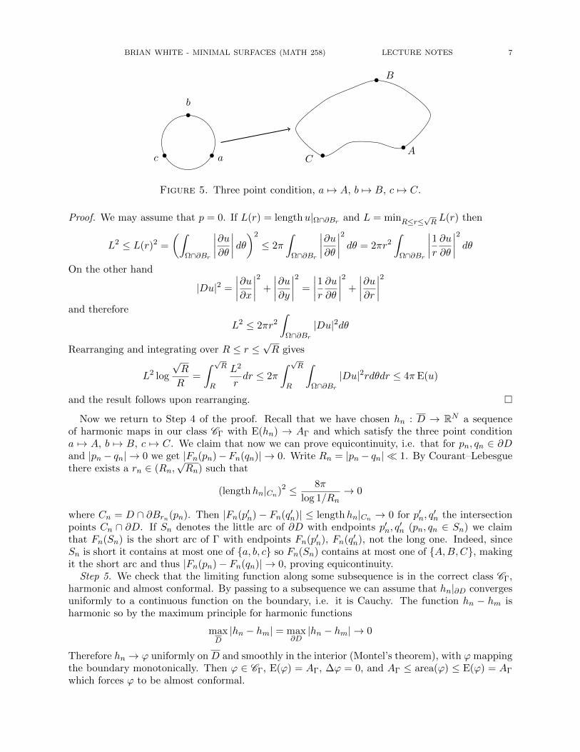
Step 4. We need to show that hn is equicontinuous on the boundary. This is actually notautomatic, so instead we impose a three point condition! Fixing a, b, c ∈ ∂D and A,B,C ∈ Γ withthe same orientation we require that a 7→ A, b 7→ B, and c 7→ C at all previous steps of the proofand invoke the Courant–Lebesgue lemma.

Lemma 2.11 (Courant–Lebesgue). Suppose Ω ⊂ R2 open, p ∈ R2, u : Ω → RN , E(u) ≤ E < ∞,

and R ∈ (0, 1) are given. Then there exists a radius r between R and√R such that(

lengthu|Ω∩∂Br(p))2 ≤ 8πE

log 1/R


•

•

• A

B

C•

•

• a

b

c

Figure 5. Three point condition, a 7→ A, b 7→ B, c 7→ C.

Proof. We may assume that p = 0. If L(r) = lengthu|Ω∩∂Br and L = minR≤r≤√R L(r) then

L2 ≤ L(r)2 =

(∫Ω∩∂Br

∣∣∣∣∂u∂θ∣∣∣∣ dθ)2

≤ 2π

∫Ω∩∂Br

∣∣∣∣∂u∂θ∣∣∣∣2 dθ = 2πr2

∫Ω∩∂Br

∣∣∣∣1r ∂u∂θ∣∣∣∣2 dθ

On the other hand

|Du|2 =

∣∣∣∣∂u∂x∣∣∣∣2 +

∣∣∣∣∂u∂y∣∣∣∣2 =

∣∣∣∣1r ∂u∂θ∣∣∣∣2 +

∣∣∣∣∂u∂r∣∣∣∣2

and therefore

L2 ≤ 2πr2

∫Ω∩∂Br

|Du|2dθ

Rearranging and integrating over R ≤ r ≤√R gives

L2 log

√R

R=

∫ √RR

L2

rdr ≤ 2π

∫ √RR

∫Ω∩∂Br

|Du|2rdθdr ≤ 4πE(u)

and the result follows upon rearranging.

Now we return to Step 4 of the proof. Recall that we have chosen hn : D → RN a sequenceof harmonic maps in our class CΓ with E(hn) → AΓ and which satisfy the three point conditiona 7→ A, b 7→ B, c 7→ C. We claim that now we can prove equicontinuity, i.e. that for pn, qn ∈ ∂Dand |pn − qn| → 0 we get |Fn(pn)−Fn(qn)| → 0. Write Rn = |pn − qn| 1. By Courant–Lebesguethere exists a rn ∈ (Rn,

√Rn) such that

(lengthhn|Cn)2 ≤ 8π

log 1/Rn→ 0

where Cn = D ∩ ∂Brn(pn). Then |Fn(p′n) − Fn(q′n)| ≤ lengthhn|Cn → 0 for p′n, q′n the intersection

points Cn ∩ ∂D. If Sn denotes the little arc of ∂D with endpoints p′n, q′n (pn, qn ∈ Sn) we claim

that Fn(Sn) is the short arc of Γ with endpoints Fn(p′n), Fn(q′n), not the long one. Indeed, sinceSn is short it contains at most one of a, b, c so Fn(Sn) contains at most one of A,B,C, makingit the short arc and thus |Fn(pn)− Fn(qn)| → 0, proving equicontinuity.

Step 5. We check that the limiting function along some subsequence is in the correct class CΓ,harmonic and almost conformal. By passing to a subsequence we can assume that hn|∂D convergesuniformly to a continuous function on the boundary, i.e. it is Cauchy. The function hn − hm isharmonic so by the maximum principle for harmonic functions

maxD|hn − hm| = max

∂D|hn − hm| → 0

Therefore hn → ϕ uniformly on D and smoothly in the interior (Montel’s theorem), with ϕ mappingthe boundary monotonically. Then ϕ ∈ CΓ, E(ϕ) = AΓ, ∆ϕ = 0, and AΓ ≤ area(ϕ) ≤ E(ϕ) = AΓ

which forces ϕ to be almost conformal.


•• ••Fn(p′n)

Fn(pn)Fn(q′n)

Fn(qn)••

•• p′nq′npnqn

Cn

Figure 6. Establishing equicontinuity at the boundary by the Courant-Lebesgue lemma.

Step 6. Interior branch points are isolated. This comes from the fact that the minimizer ϕ is aharmonic function on D and therefore for z = x+ iy and the differentials

∂

∂z=

1

2

(∂

∂x− i ∂

∂y

)and

∂

∂z=

1

2

(∂

∂x+ i

∂

∂y

)we see that

∆ϕ = 0⇔ ∂

∂z

∂ϕ

∂z= 0⇔ ∂ϕ

∂zis holomorphic

Recall that zeros of holomorphic functions are isolated and the result follows.

With a slightly more refined argument the precise version of the theorem we can get is:

Theorem 2.12. Suppose F : D → RN represents a classical minimal disk: F : D → RN iscontinuous, F : ∂D → Γ is continuous and monotone, ∆F = 0, F is almost conformal, andarea(F ) (= E(F )) < ∞. If k ≥ 1 and Γ is Ck,α then F |D is Ck,α too. In particular if Γ is smooth

then F : D → RN is smooth as well. Also p ∈ D : DF (p) is a finite set, i.e. branch points areisolated.

Remark 2.13. As a reminder, in the case N = 3 it has been shown [Gul73] that there can be nointerior branch points. The existence of boundary branch points in R3 is an open problem.

3. Douglas Theorem for Surfaces of Higher Genus

In this lecture we seek to extend the Douglas-Rado theorem to surfaces whose topology is morecomplicated than that of a disk. To this end there is the following theorem by Douglas [Dou39a].

Theorem 3.1 (Douglas Theorem for Annuli). Suppose there exists an annulus with boundaryΓ1 ∪ Γ2, where Γ1, Γ2 are disjoint oriented simple closed curves in RN , whose area is smallerthan that of any pair of disks (“Douglas condition”). Then there exists a radius R ∈ (1,∞) and acontinuous map F : A(1, R) → RN , A(1, R) = p ∈ R2 : 1 ≤ |p| ≤ R, such that ∆F = 0, F isalmost conformal, F : ∂A(1, R) → Γ1 ∪ Γ2 monotonically such that area(F ) (= E(F )) is the leastpossible area among annuli.

Proof. The proof is more or less the same as before, the only catch being that we have no controlover the optimal radius R because different annuli A(1, R) are not conformally equivalent. Pick aminimizing sequence Fi : A(1, Ri) → RN with E(Fi) decreasing to the infimum of areas. Withoutloss of generality Fi is harmonic. In order to pass to a subsequence and argue as before, we needto check that Ri is bounded away from 1 and ∞.

Step 1. Ri stays away from 1. If we were to have Ri → 1 along some subsequence then we couldargue that E(Fi)→∞ in a way similar to before. This gives a contradiction.

Step 2. Ri stays away from ∞. Recall that we have a uniform upper bound E(Fi) ≤ E < ∞.Then by Courant-Lebesgue there exist ri ∈ (1, Ri) such that lengthFi|∂Bri → 0. We can perform


A(1, R)

Γ1

Γ2

Figure 7. Plateau problem for annuli

Fi(∂Bri)

Figure 8. Split the narrow neck into two disjoint disks.

surgery and split up the narrow neck into two small disjoint disks that are filled up. Then weget a pair of disk solutions to the Plateau problem whose area converges to the infimum, whichcontradicts the Douglas condition.

Remark 3.2. As the narrow neck picture above suggests, one way to get the Douglas condition isfor Γ1,Γ2 to be “close together” with the “same orientation.”

The proof similarly extends to mappings from surfaces of higher genus. The statement is:

Theorem 3.3 (Douglas Theorem for Higher Genus, [Dou39a]). Suppose Γ is a smooth embeddedclosed curve (not necessarily connected). For each g <∞ there exists a least area genus ≤ g surfacethat solves the Plateau problem for Γ.

Theorem 3.4 (Alternative Formulation of the Douglas Theorem). Let Γ be as above. If Ak denotesthe infimum of areas among surfaces of genus k with boundary Γ then trivially A0 ≥ A1 ≥ . . . andif Ag < Ag−1 (“Douglas condition”) then there exists a least area genus g surface.

4. Intersections of Minimal Surfaces, Meeks-Yau Theorem

In this lecture we studied (self-)intersections of minimal surfaces in R3 (or more generally in3-manifolds) and the question of whether or not the solution to the Plateau problem is embedded.We start off with an application of Douglas’s higher genus theorem.

Theorem 4.1. Suppose that in the Douglas theorem we have Ag−1 > Ag = Ag+1 in R3 and thatM is a least area genus g surface with ∂M = Γ. Then M does not intersect itself transversely inits interior.

Proof. Suppose that M intersected itself transversely on at least one point. If p ∈ M is the pointwhere two sheets of M meet transversely, we can perform surgery around p and add a handlebetween the different sheets and smoothing as in Figure 9. This gives a genus g + 1 surface withsmaller area, a contradiction.

Remark 4.2. This gives a sufficient hypothesis for the “Douglas condition.” If we have a genusg minimizer which crosses itself then we can construct a genus g + 1 surface with strictly smallerarea thus guaranteeing Ag > Ag+1.


Figure 9. Constructing a higher genus surface with smaller area due to transverse intersection.

One reason regularity of solutions to the Plateau problem in R3 is simpler than regularity inRN in general is because minimal surfaces intersect in predictable ways in R3 and 3-manifolds ingeneral. The following theorem helps quantify this statement.

Theorem 4.3. Suppose M , M ′ are smooth embedded minimal surfaces in R3 (or a 3-manifold).Suppose M , M ′ are tangent at a point p. Then for some neighborhood U of p either (1) the surfacesoverlap, i.e. M ∩U = M ′ ∩U , or (2) (M ∩M ′)∩U consists of k curves that meet at k equal anglesat p (k − 1 being the order of contact) and the point p of tangency is isolated.

Proof. (In the special case of M ′ being the horizontal plane in R3.) Suppose our surface M is(locally) parametrized by F : D → R3 so that F is harmonic and conformal. If f is the thirdcoordinate of F then f is harmonic too and M ∩M ′ = F (f = 0), f(0) = 0, Df(0) = 0. Theneither f ≡ 0, which is case (1), or f = Re

(a0z

Q + a1zQ+1 + . . .

)for Q ≥ 2. We may change

coordinates conformally and assume f = Re(zQ(1 + a1z + . . .)

). For z near 0 we can perform yet

another conformal change of coordinates w = z(1 + a1z + . . .)1/Q by fixing a choice of Q-th roots,in which case M ∩M ′ locally consists of points Re

(wQ)

= rQ sinQθ, which is case (2).

Corollary 4.4. If M , M ′ are two smooth embedded minimal surfaces in a 3-manifold N3, andX = p : M ∩ U = M ′ ∩ U for some neighborhood U of p, then X is simultaneously both closedand open in (M ∪M ′) \ (∂M ∪ ∂M ′).

Proof. Clearly X is open by definition, so it suffices to show its complement is open too. If q is inthe complement then it is either not in M or not in M ′, which is an open condition, or at worse itis an isolated tangency point with curves of transverse intersection leading into it by the previoustheorem, which is also an open condition.

This corollary allows us to prove that area minimizing disks are disjoint provided they merelystay away from each others’ boundary.

Theorem 4.5. Suppose M , M ′ are least area embedded disks in N3. Suppose, further, that theydo not intersect at boundary points in the sense that ∂M ∩M ′ = M ∩ ∂M ′ = ∅. Then M and M ′

are disjoint.

Proof. First, M and M ′ cannot overlap anywhere because by the corollary the overlap would extendto the boundary. Consequently M ∩M ′ consists of finitely many points that are joined by smoothcurves. By elementary graph theory, M ∩M ′ contains a closed curve. We claim this contradictsthe area minimizing nature of M , M ′. Indeed suppose Σ, Σ′ are the regions of M , M ′ that arebounded by the common closed curve. Then area(Σ) = area(Σ′), otherwise one could reduce thearea of either M or M ′ by replacing the region of larger area by the region of smaller area. Butnow (M \ Σ) ∪ Σ′ is an area minimizing disk which is not smooth, a contradiction.


M

M ′Σ

Σ′

Figure 10. Intersection of two embedded minimal surfaces in a 3-manifold.

Remark 4.6. In reality we have only proved in previous lectures that the solution we constructedis smooth, not that any area minimizing solution is smooth. But this does hold, for example inthis case by Osserman’s theorem.

There are certain situations in which we can guarantee that our surfaces stay away from eachothers’ boundary. For example we may make use of the following lemma:

Lemma 4.7 (Convex Hull Property). If F : D → RN is continuous and ∆F = 0, then F (D) iscontained in the convex hull of F (∂D). Furthermore, interior points get mapped to points in theinterior of the convex hull

Proof. The convex hull is the intersection among all half-spaces containing F (∂D). If ν is thenormal to the half-space, the maximum of F · ν is attained on ∂D so F never leaves any one ofthose half-spaces. The interior point claim follows from the strong maximum principle.

Corollary 4.8. If M , M ′ are minimal surfaces in the unit ball B1 ⊂ R3 such that ∂M and∂M ′ ⊂ ∂B1, and also ∂M ∩ ∂M ′ = ∅, then ∂M ∩M ′ = M ∩ ∂M ′ = ∅.

The next result we will state but not prove generalizes Dehn’s lemma which was stated in 1910and proved in 1957 in [Pap57a], [Pap57b]. This result is due to Meeks and Yau and (using thelemma above) proves in full generality a conjecture due to Osserman, which we state as its corollary.

Theorem 4.9 (Meeks-Yau Theorem, [MY80]). Suppose F : D → N3 is a least area disk with F |∂Dan embedding, F (∂D) = Γ a simple closed curve. Suppose F−1(Γ) = ∂D, i.e. no interior pointgets mapped to Γ. Then F is a smooth embedding.

Corollary 4.10 (Osserman’s conjecture). Let Γ be a simple closed curve on the boundary of theunit ball in R3, i.e. Γ ⊂ ∂B1 ⊂ R3. Let F : D → R3 be the least area disk mapping ∂D to Γ. ThenF is a smooth embedding.

5. Branch Points

Recall that a branch point is locally modeled by F : D ⊂ R2 ' C → C × RN−2 ' RN whereF (0) = 0 and DF (0) = 0. If F is minimal, we can expand it in a power series, and write F (z) =(zQ, 0) + o(zQ). By a non-conformal change of coordinates, we may assume that F (z) = (zQ, f(z))for some function f . Hence, we have written this as a “multivalued graph,” i.e. if we let w = zQ,we’re considering the “graph” of f(w1/Q) (we won’t take this point of view, but it’s useful to keepin mind). At this point we can distinguish between “false” and “true” branch points.

False branch points. It is entirely possible that f(z) = ψ(zQ) for some ψ. In this case, the graphof F is the same as the graph of ψ and the surface was actually smooth, only the parametrizationwas bad.

True branch points. These are simply all the branch points that are not false. Relevant to these is

Theorem 5.1 (Osserman [Oss70]). If F : M2 → Nn is almost conformal and harmonic (i.e.minimal) and if F has a true interior brach point at p ∈M , then F is not area minimizing.


• •

Figure 11. Examples of false branch points (left) and true branch points (right).

Proof. There exists a curve of transverse self intersection going to a branch point as in Figure 12.In particular, we could attempt to apply the same handle attaching argument as in Figure 9, which

F (p)

Figure 12. A curve of self-intersection near a branch point.

would in fact decrease the area. However, we cannot use this exact argument, as it could potentiallyraise the genus of the surface, which would not prove anything. Osserman’s key observation wasthat in the branch point case, we can decrease the area without changing the topology. Osserman’s

p

old

old

newnew

Figure 13. Osserman’s area decreasing modification of a surface with a branch point.

gluing argument is illustrated in Figure 13, but essentially the idea is that because p is a branch


point, there are at least two preimages of the curve of self intersection found above Then, by aclever gluing argument, one may show that by gluing the surface along these curves, it is possibleto decrease the area without changing the topology.

6. First Variation and Monotonicity Formulae

Suppose that Mm ⊂ Nn is a submanifold. We’ll consider variations of M , i.e. a family ft :Mm → Nn so that f0(x) ≡ x along M . We’d like to compute d

dt

∣∣t=0

area(ft(M)). First, recall that

area(ft(M)) =

∫M| Jac(ft)|dx =

∫M

√det(Dft)TDftdx,

and assuming everything is smooth enough, we thus have that (using the fact that f0 is an isometry,so Df0 = Id)

d

dt

∣∣∣t=0

area(ft(M)) =

∫M

d

dt

∣∣∣t=0

√det(Dft)TDftdx

=

∫M

1

2√

det ((Dft)TDft) |t=0

d

dt

∣∣∣t=0

det((Dft)

TDft)

=1

2

∫M

tr

(d

dt

∣∣∣t=0

(Dft)TDft

)dx

To calculate this, we first define a vector field by X(x) := ddt

∣∣t=0

ft(x). In normal coordinates p

around a point, we know that Dft =(∂(ft)j

∂xi

)i=1,...,m,j=1,...n

, so

tr

(d

dt

∣∣∣t=0

((Dft)

TDft))

=

m∑i=1

n∑k=1

d

dt

∣∣∣t=0

(∂(ft)

k

∂xi

)2

= 2

m∑i=1

n∑k=1

∂(f0)k

∂xi∂Xk

∂xi

= 2

m∑i=1

ei · ∇eiX.

In particular, this shows that

d

dt

∣∣∣t=0

area(ft(M)) =

∫M

divM X dx.

This is one version of the formula for the first variation of area. We will now derive severalrelated versions which are also of much importance. By splitting up X into its component whichis tangential to M , denoted XT and component which is normal to M , denoted X⊥, we have that∫

MdivM X =

∫M

divM X⊥ +

∫M

divM XT

First, by Stoke’s theorem, we have that∫M

divM XT =

∫∂M

XT · ν =

∫∂M

X · ν


where ν is the (outward) pointing unit normal of ∂M . We have also used the fact that ν ∈Γ(∂M, TM), so ν ·X⊥ = 0. On the other hand, we have that

divM X⊥ =m∑i=1

ei · ∇eiX⊥

=

m∑i=1

∇ei(ei ·X⊥︸︷︷︸=0

)− (∇eiei) ·X⊥

= −m∑i=1

II(ei, ei) ·X⊥

= −H ·X⊥

= −H ·X,where we have defined the mean curvature H to be the trace of the second fundamental form, asabove. As such, we may rewrite the first variation formula as

d

dt

∣∣∣t=0

area(ft(M)) =

∫M

divM X dx = −∫MH ·X +

∫∂M

X · ν.

In particular, if H 6= 0 at some point in the interior of M , we may find a vector field so thatX ·H > 0 near the point and X ·H = 0 away from the point, so d

dt

∣∣t=0

area(ft(M)) < 0. Thus, ifM is area minimizing, then necessarily H = 0. In particular, we define

Definition 6.1. A submanifold M is minimal if and only if ddt

∣∣t=0

area(ft(M)) = 0 for all compactlysupported variations X ∈ Γ(M\∂M, TN). Equivalently, this holds if and only if H ≡ 0.

Now we want to establish the monotonicity formula. Suppose that M is a compact minimalsubmanifold of RN . Let X(x) = ~x. It is not hard to check that divM X = m. In particular, thefirst variation formula yields

m area(M) =

∫∂M

X · νM ds.

On the other hand, let C = 0

#

∂M (the cone over ∂M with respect to the origin) as illustrated

0

∂M

Figure 14. The cone over ∂M .

in Figure 14. The first variation formula also yields

m area(C) = −∫CHC ·X +

∫∂M

X · νcone.

However, because X is tangent to C, the first term vanishes. Furthermore, we claim that

X · νM ≤ X · νcone.To see this, for p ∈ ∂M consider W ⊂ TpRN the two dimensional subset which is normal to Tp∂M .We claim that among all unit vectors ~n ∈W , X · ~n is maximized at νcone. To see this, note that

‖X‖2 ≥ ‖projTp∂M⊕〈~n〉X‖2 = ‖ projTp∂M X‖2 + ‖ proj〈~n〉X‖2 = ‖projTp∂M X‖2 + | 〈~n,X〉 |,


However, because Tp∂M ⊕〈νcone〉 = TpC, it is clear that for ~n = νcone, we have equality in the firstinequality above. This proves the claim.

As such, we see that

area(M) ≤ area(C).

This allows us to derive the monotonicity formula as follows. Let A(r) = area(M ∩ Br(p)). For0 < r < dist(p, ∂M), we have that

A′(r) ≥ L(r) = L(∂(Br(p) ∩M)) = L(M ∩ ∂Br(p)).The first inequality follows from the co-area formula. On the other hand, above formula impliesthat

A(r) ≤ area(0

#

(M ∩ ∂Br(p))) =r

mL(r).

Thus A′(r) ≥ mr A, and integrating this we have

Theorem 6.2 (Monotonicity Formula). For M a minimal surface, the quantity

area(M ∩Br(p))rm

is an increasing function of r for 0 < r < dist(p, ∂M). Furthermore, the quantity is strictlyincreasing unless M is a cone with vertex p.

We may define

Θ(M,p, r) :=area(M ∩Br(p))

ωmrm

where ωm is the area of the unit m-ball. The monotonicity formula is equivalent to the claim thatΩ(M,p, r) is an increasing function of r for r < dist(p, ∂M).

In fact, letting Ep = λ(x − p) + p : x ∈ ∂M, λ ≥ 1 denote the exterior cone over ∂M withrespect to p, the same proof as above shows

Theorem 6.3 (Extended Monotonicity Formula, Ekholm–White–Wienholtz [EWW02]). The den-sity Θ(M ∪ Ep, p, r) is increasing for r ∈ (0,∞).

This allows us to discuss the “density at infinity” for minimal submanifolds of RN .

Theorem 6.4. For M a minimal submanifold of RN with ∂M = ∅ or ∂M compact and M un-bounded, the density at infinity, defined by

Θ(M) := limr→∞

Θ(M,p, r)

is well defined independently of the choice of p and furthermore Θ ≥ 1.

Proof. We first note that we may replace M by M\BR(p) for R so that ∂M ⊂ BR(p) and ∂BR(p)intersects M transversely (as it does for a.e. R) and as such, may assume that ∂M is smooth.

Let Ep be the exterior cone of ∂M with respect to p. By the extended monotonicity formula, wehave that Θ(M ∪ Ep, p, r) is an increasing function of r ∈ (0,∞). Thus, we have that

limr→∞

Θ(M ∪ Ep, p, r)

exists. Furthermore, for large r, letting C = 0

#

∂M ,

Θ(M ∪ Ep, p, r) = Θ(M,p, r) + Θ(Ep, p, r) = Θ(M,p, r) + Θ(C, p, r) + Θ(Ep\C, p, r).It is clear that Θ(C, p, r) is independent of r and Θ(Ep\C, p, r)→ 0 as r →∞, as it has finite totalarea. This shows that the limit defining Θ(M) exists. To see that it is independent of the choiceof point p, notice that

M ∩Br(p) ⊆M ∩Br+|p−q|(q),


so from this we see that

area(M ∩Br(p))ωmrm

≤area(M ∩Br+|p−q|(q)

ωmrm=

area(M ∩Br+|p−q|(q)ωm(r + |p− q|)m

(r + |p− q|

r

)m.

Taking the limit as r →∞, we see that

Θ(M,p,∞) ≤ Θ(M, q,∞)

but we could clearly reverse the role of p and q. This shows that Θ(M) does not depend on thechoice of point p.

Finally, it remains to show that Θ ≥ 1. If ∂M = ∅, this follows easily from taking p ∈ M andusing the monotonicity formula (it is not hard to check that limr→0 Θ(M,p, r) ≥ 1). On the otherhand, if ∂M 6= ∅, by assumption there exists q ∈ M which is a distance R 1 away from ∂M .The extended monotonicity formula implies that

Θ(M ∪ Eq, q, r) ≥ limt→0

Θ(M ∪ Eq, q, t) ≥ 1.

On the other hand, taking r →∞, we see that

Θ(M) + Θ(Eq) ≥ 1.

By the same argument as above, we see that Θ(Ep) = Θ(C). However, as R → ∞ the cone angletends to 0, and as such Θ(C)→ 0. This shows that Θ(M) ≥ 1.

7. Limits of Minimal Surfaces

Suppose that Mi ⊂ Ω is a sequence of minimal submanifolds of some open set Ω with ∂Mi ⊂ ∂Ω.Can we take the limit of the Mi? Can singularities arise in the limit? We address these questionshere, proving a sequence of theorems.

Theorem 7.1. If the Mi are minimal surfaces and each Mi = graph(fi : Bm → RN−m) with‖fi‖C2 ≤ C <∞ then, up to extracting a subsequence, the fi converge smoothly on compact subsetsof Bn to f so that M = graph(f) is a minimal surface.

Proof. By the Arzela-Ascoli theorem, we may extract a subsequence so that fi → f in C1,α oncompact sets. Now, an easy PDE argument (using Schauder estimates for linear elliptic equations)shows that we may in fact upgrade this convergence to smooth convergence on compact sets. It iseasy to see that the limiting function has its graph a minimal surface.

For the next convergence theorem, for a minimal surface M and point p ∈M , we define |A|(M,p)to be the norm of the second fundamental form of M at p. We note that from now on, one couldassume that Ω is a domain in a Riemannian manifold as the above theorem will still hold locallynear a point (the manifold is approximately flat on small scales). However, we will not worry toomuch about this remark.

Theorem 7.2. For Mi ⊂ Ω a sequence of minimal submanifolds with ∂Mi ⊂ ∂Ω, if |A|(Mi, ·) isuniformly bounded on compact subsets of Ω and we have the area bound for K b Ω, area(M ∩K) ≤AK <∞, then up to a subsequence, the Mi converge smoothly to some minimal surface M .

Proof. We’d like to apply the previous theorem. Choose pi ∈Mi∩K. Extracting a subsequence, thepi converge to some p. We may further assume that Tan(Mi, pi)→ T for some plane T . Then, wemay express the surfaces Mi locally as graphs (a bounded number, by the area bounds) over T (bythe bound on the second fundamental form) and use the above theorem to extract a subsequence.Then, a diagonal argument allows us to find a sequence converging smoothly on all of Ω.

However, what if we don’t have second fundamental form bounds? Then, we should expect thepossibility of singularities forming. The following theorem helps us have a better understanding ofhow this happens


Theorem 7.3. If Mi ⊂ Ω are minimal with ∂Mi ⊂ ∂Ω, suppose that |A|(Mi, ·) has a local maximumat a sequence of points pi, converging to some p ∈M . Suppose further that |A|(Mi, pi)→∞. Then,letting λi := |A|(Mi, pi) the blown up surfaces λi(Mi − pi) converge smoothly to a minimal surfaceM ⊂ RN with ∂M = ∅. Furthermore, |A|(M, ·) ≤ |A|(M, 0) = 1.

Proof. Letting M ′i := λi(Mi − pi), it is not hard to check by scaling that |A|(M ′i , ·) ≤ 1. Then, theprevious theorem guarantees the desired convergence.

An example of this is given by the catenoid, as in Figure 15. If we scale the catenoid down by

z

p

z = cosh−1 r

Figure 15. The catenoid. The point p is a local maximum for |A|(·).

1n , then it converges to two planes (away from the origin). However, the curvature is blowing up

at the points 1np which are converging to the origin. Performing the rescaling above will just lead

to the catenoid again, which is a simple example of what is possible to get as a rescaling limit inthe above theorem.

Finally, one might wonder what happens if there is no local maxima of |A|(·)? It turns out thatby using a point-picking argument, we can still attain a good blowup limit

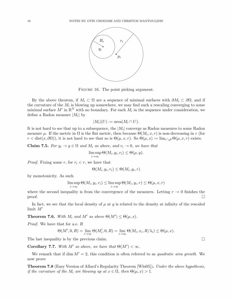
Theorem 7.4. For Mi ⊂ Ω minimal with ∂Mi ⊂ ∂Ω, assume that pi ∈ Mi with pi → p ∈ Ω have|A|(Mi, pi)→∞. Then, there exists (up to a subsequence) new points qi ∈Mi with qi → p so thatfor λi := |A|(Mi, qi), λi(Mi − q1) converges smoothly to M a smooth minimal submanifold of RNwith no boundary and |A|(M, ·) ≤ |A|(M, 0) = 1.

Proof. Let ri < dist(p, ∂Ω) tend to zero slowly enough so that still ri|A|(Mi, pi) → ∞ (e.g. one

could take ri := |A|(Mi, pi)−1/2). We’ll choose qi ∈Mi ∩Bri(pi) to maximize

|A|(Mi, ·) dist(·, ∂Bri(pi)).Letting Ri := dist(qi, ∂ri(pi), notice that qi also automatically maximizes

|A|(Mi, ·) dist(·, ∂BRi(qi))on Mi ∩ BRi(qi). This is because dist(·, ∂BRi(qi)) ≤ dist(·, ∂Bri(pi)) here. See Figure 16. Now,we see that |A|(Mi, qi)Ri ≥ |A|(M,pi)ri → ∞, and Ri ≤ ri → 0. In particular, we may defineλi := |A|(Mi, qi) and M ′i = λi(Mi− qi). Because |A|2 ∗dist is a scale invariant quantity, we see that

|A|(M ′i , x) dist(x, ∂BλiRi(0)) ≤ λiRi,by the above choices. As such,

|A|(Mi, x) ≤ λiRiλiRi − |x|

→ 1

as i→∞. Thus, the same argument as in the previous theorem yields the desired conclusion.


ri

pi

qi

Ri

Figure 16. The point picking argument.

By the above theorem, if Mi ⊂ Ω are a sequence of minimal surfaces with ∂Mi ⊂ ∂Ω, and ifthe curvature of the Mi is blowing up somewhere, we may find such a rescaling converging to someminimal surface M ′ in RN with no boundary. For each Mi in the sequence under consideration, wedefine a Radon measure |Mi| by

|Mi|(U) := area(Mi ∩ U).

It is not hard to see that up to a subsequence, the |Mi| converge as Radon measures to some Radonmeasure µ. If the metric in Ω is the flat metric, then because Θ(Mi, x, r) is non-decreasing in r (forr < dist(x, ∂Ω)), it is not hard to see that so is Θ(µ, x, r). So Θ(µ, x) := limr0 Θ(µ, x, r) exists.

Claim 7.5. For yi → y ∈ Ω and Mi as above, and ri → 0, we have that

lim supi→∞

Θ(Mi, yi, ri) ≤ Θ(µ, y).

Proof. Fixing some r, for ri < r, we have that

Θ(Mi, yi, ri) ≤ Θ(Mi, yi, r)

by monotonicity. As such

lim supi→∞

Θ(Mi, yi, ri) ≤ lim supi→∞

Θ(Mi, yi, r) ≤ Θ(µ, x, r)

where the second inequality is from the convergence of the measures. Letting r → 0 finishes theproof.

In fact, we see that the local density of µ at y is related to the density at infinity of the rescaledlimit M ′

Theorem 7.6. With Mi and M ′ as above Θ(M ′) ≤ Θ(µ, x).

Proof. We have that for a.e. R

Θ(M ′, 0, R) = limi→∞

Θ(M ′i , 0, R) = limi→∞

Θ(Mi, xi, R/λi) ≤ Θ(µ, x).

The last inequality is by the previous claim.

Corollary 7.7. With M ′ as above, we have that Θ(M ′) <∞.

We remark that if dimM ′ = 2, this condition is often referred to as quadratic area growth. Wenow prove

Theorem 7.8 (Easy Version of Allard’s Regularity Theorem [Whi05]). Under the above hypothesis,if the curvature of the Mi are blowing up at x ∈ Ω, then Θ(µ, x) > 1.


Proof. By the above theorem, we know that Θ(M ′) ≤ Θ(µ, x). On the other hand,

1 ≤ Θ(M ′, 0) ≤ Θ(M ′)

by monotonicity, with equality in the second inequality if and only if M ′ is a cone centered at 0.Because M ′ is smooth, this can only be true if it is a union of planes through the origin, whichcannot be true as M ′ is not flat, by construction.

In fact, we can improve this slightly

Theorem 7.9 ([Whi05]). There is ε = ε(n,N) so that if M ′ is a complete, minimal n-dimensionalsurface in RN with |A|(M ′, ·) ≤ |A|(M ′, 0) = 1, then Θ(M ′) ≥ 1 + ε.

Proof. Let α := infΘ(M ′) : M ′ as in theorem. We may assume α < ∞. As such, we choosea minimizing sequence M ′i with Θ(M ′i) → α. Passing to a subsequence, the curvature boundsguarantee smooth convergence to some M ′ (with maximal curvature 1 at the origin). As such, fora.e. R, we have that

Θ(M ′, 0, R) = limi→∞

Θ(M ′i , 0, R) ≤ limi→∞

Θ(M ′i) = α.

Because M ′ is non-flat, we thus see that 1 < Θ(M ′) = α, as desired.

One might wonder if there is always equality in Theorem 7.6. An example of strict inequality isprovided by the Costa–Hoffman–Meeks surfaces, cf. [HM85].

Figure 17. A Costa–Hoffman–Meeks surface along with the limiting catenoid and plane

These are a sequence of embedded minimal surfaces Mg which are of genus g and are asymptoticto a catenoid and a plane. In particular, as the genus tends to ∞, the curvature is blowing up ona circle. The surfaces along with their limit as the genus tends to infinity are illustrated1 in Figure17. On the other hand, the rescaled surfaces 1

gMg converge to a multiplicity three plane. As such,

writing µ for the limit, Θ(µ, 0) = 3. However, rescaling to obtain a smooth limit, one finds Scherk’ssingly periodic surface, which looks like the union of two planes, and as such has density at infinity2.

The following exercises are “true,” by GMT methods, but it is not clear how to solve them usingclassical minimal surface methods

Exercise 1. If M ′ is a minimal surface with dimM ′ = 2, if Θ(M ′) <∞, show that Θ(M ′) ∈ N. Aspecial case is to show that α := minΘ(M ′) : M ′ is not flat = 2.

1Thanks to David Hoffman for providing these pictures.


A roughly equivalent problem is

Exercise 2. Suppose that Mi are minimal surfaces (two dimensional) and |Mi| → µ as Radonmeasures. Suppose further that there is a 2-plane P so that µ = θ|P |. Show that θ ∈ N.

8. Genus and Total Curvature of Minimal Surfaces

We define the genus of a surface (possibly non-compact) as follows: first we use the classicaldefinition for closed surfaces. Secondly, we demand that the genus is additive in the usual way,and finally we define the genus for a compact surface with boundary to be the genus of the surfaceformed by capping off each boundary component.

This definition is quite well behaved with respect to the discussion of the previous section.In particular, if dimMi = 2, Mi ⊂ Ω and ∂Mi ⊂ ∂Ω are a sequence of minimal surfaces whosecurvatures are blowing up, then if genus(Mi) ≤ g, this implies that genus(M ′) ≤ g (where M ′ is thesurface obtained as in the previous section by blowing up the parts with concentrating curvature toobtain a smooth limit). In fact, the same thing holds even if we only require genus(Mi∩Bε(x)) ≤ g,where x is the point of curvature blowup.

As such, we’re naturally led to the study of blowups M ′ with finite genus. Our main results are

Theorem 8.1. Suppose that M is a two dimensional complete, properly immersed (without bound-ary) minimal surface with quadratic area growth and finite genus. Then∫

M|K| dA <∞,

i.e. M has finite total curvature.

Remark 8.2. Suppose we have a surface M2 ⊂ R3 with principal curvatures κ1, κ2. Then themean curvature is H = κ1 + κ2 and the Gauss curvature K = κ1κ2. In particular

K =H2

2− |A|

2

2

If M is minimal then K = −12 |A|

2 and |K| = 12 |A|

2. In particular, the theorem guarantees we have

global L2 finiteness of the curvature norm.

In the converse direction we have the following theorem due to Osserman (in R3) and Chern-Osserman (in RN , N ≥ 4):

Theorem 8.3 (Osserman [Oss64], Osserman-Chern [CO67]). Suppose M2 ⊂ RN is a completeorientable (without boundary) minimal surface with finite total curvature; i.e.∫

M|K| dA <∞

Then(1) M is conformally equivalent to a closed surface Σ with finitely many points removed (and

hence has finite genus),(2) the Gauss map p 7→ TpM extends continuously to Σ,(3) The Gauss curvature integrates to an integer multiple of 4π (in R3) or 2π (for N ≥ 4), i.e.

−∫MK dA =

∫M|K| dA =

4πj for N = 3

2πj for N ≥ 4

(4) M is proper in RN and exhibits quadratic area growth.


There are various things we can say before turning to the proof of either theorem. For starters,note that surfaces with quadratic area growth and which are properly immersed form a naturalclass of surfaces to study, because all rescaling limit surfaces M ′ turn out to be such. We alreadyknow they exhibit quadratic area growth from Corollary 7.7, but why are they properly immersed?It turns out to be a consequence of area growth and our pointwise curvature bounds:

Lemma 8.4. Suppose M2 ⊂ RN is a minimal surface (without boundary) such that Θ(M) < ∞and whose pointwise curvature is uniformly bounded. Then M is properly immersed.

Proof. Suppose pi ∈ M is a sequence of points that escapes to infinity intrinsically but not ex-trinsically. In view of our uniform curvature bounds around each pi there exists a ball of fixedradius in which M looks like a graph. After passing to a subsequence we may assume that the piaccumulate to some q ∈ Rn and that on slightly smaller balls the graphs converge smoothly to acommon graph. This contradicts finiteness of area in a neighborhood of q.

. p1 . p2 . . . . q

Figure 18. Illustration of the contradiction obtained by the existence of accumu-lation points.

Before proceeding to the proof of the first main theorem, we present an application of themonotonicity formula which forces a bound on just how spread out the boundary of a minimalsurface can be in terms of its length.

Lemma 8.5. Let M2 ⊂ RN be a compact minimal surface with boundary ∂M . Then

maxp∈M

distRN (p; ∂M) ≤ length(∂M)

2π

Equality is attained if and only if M is a planar disk.

Proof. Let p ∈ M \ ∂M , Ep denote the exterior of the cone p

#

∂M , and C denote the full cone.By the extended monotonicity formula

1 ≤ Θ(M,p) ≤ Θ(M ∪ Ep, p,∞) = Θ(C, p,∞)

If r = dist(p; ∂M) and π : RN \ p → ∂B1(p) denotes the standard projection function theninvariance of C under dilations gives

Θ(C, p,∞) =length(π(∂M))

2π≤ length(∂M)

2πr

and the result follows by rearranging r and taking the supremum over all p ∈M .

Remark 8.6. There exists an analogous statement for higher dimensional minimal surfaces Mm

in RN . It gives

maxp∈M

distRN (p; ∂M) ≤(H m−1(∂M)

) 1m−1

mωm

Here H m−1 denotes (m − 1)-dimensional Hausdorff measure and ωm the total volume of the theunit ball in Rm.


Corollary 8.7. Suppose that M2 ⊂ RN is as above, connected, and such that ∂M = Γ1 ∪ Γ2, fora pair of curves Γ1, Γ2. Then

distRN (Γ1,Γ2) ≤ length(∂M)

π

Proof. Let d = distRN (Γ1,Γ2), pick a point p ∈M that is at least d/2-apart from both Γ1, Γ2, andapply the lemma.

With these tools at hand we can return to the proof the first main theorem.

Proof of Theorem 8.1. Let us first do an easy special case to get some intuition; suppose that Mis simply connected. Pick p ∈M and let

M(r) = x ∈M : distM (x, p) ≤ r ⊂ Br(p)A(r) = area(M(r))

L(r) = length(∂M(r))

Since K < 0, ∂M(r) is a smooth curve for all r, and A′(r) = L(r). Differentiating again and usingthe first variation formula and Gauss-Bonet

A′′(r) = L′(r) =

∫∂M(r)

k ds = 2π −∫M(r)

K dA = 2π +

∫M(r)

|K| dA

Quadratic area growth (on the ambient space) forces quadratic area growth intrinsically. Since A′′

above is monotone, it must be uniformly bounded and letting r →∞ we get an L1 bound on |K|.Now let’s do the general case, with M not necessarily a disk. It is clear that there are finitely

many ends because each end must contribute at least 1 to the density at infinity by Theorem6.4. From topology we know that such 2-manifolds with finitely many ends and finite genus arehomeomorphic to closed surfaces with finitely many points removed. Thus, each end is annular.

For E an annular end and homotopic curves Γ ∼ Γi in E with Γi →∞, the corollary shows thatlength(Γi)→∞. That is, ends grow wider as they escape to infinity. At this point we may replaceΓ by the shortest curve in M homotopic to Γ because the lengths diverge as we escape to infinity.This choice of Γ is geodesic in M .

...

...

E(r)Γ Γ(r)

Figure 19. Intrinsic area growth on an annular end E.

As before let’s defineE(r) = x ∈ E : distM (x,Γ) ≤ rΓ(r) = ∂E(r) \ Γ

A(r) = area(E(r))

L(r) = length(∂E(r))


In view of K < 0, Γ(r) is smooth still, and by the same computation as above A′(r) = L(r) and

A′′(r) = L′(r) =

∫Γ(r)

k ds+

∫Γk ds

The curve Γ is geodesic so k ≡ 0. By Gauss-Bonet and the vanishing characteristic of E(r):

A′′(r) = −∫E(r)

K dA =

∫E(r)|K| dA

on each end. Our quadratic area growth assumption in turn forces an upper bound on A′′(r) andthus finiteness on total curvature in E, as before. The result follows since we have finitely manyends and the remainder of M is compact.

Proof of Theorem 8.3. The first part of the theorem is true in a very general setting; indeed Huber[Hub57] showed that any complete surface M2 ⊂ RN such that∫

M|K−| dA <∞

(where K− denotes the negative part of curvature) is conformally equivalent to a closed surface Σwith finitely many points removed.

The rest of the proof we present in the convenient special case N = 3. Equivalent to p 7→ TpMin this case is the map ~n : M → S2, ~n(p) being a unit normal to M at p. It is standard thatK = Jac~n and therefore by the area formula

area(~n(U)) =

∫U|K| dA

provided the area on the left accounts for multiplicity. Let p be one of the punctures. Choose E tobe a neighborhood with small total curvature, say∫

E|K| dA < 2π

Then area(~n(E)) < 2π < area(S2), so in particular ~n(E) misses at least three distinct pointsq1, q2, q3 ∈ S2. On the other hand ~n : E → S2 ∼= C ∪ ∞ is conformal and without loss ofgenerality q3 corresponds to ∞ on the Riemann sphere, so by Picard’s theorem ~n : E → S2 ismeromorphic and therefore extends to a holomorphic function ~n : E ∪ p → S2.

Remark 8.8. The precise nature of ~n on minimal surfaces is that of a conformal, orientation-reversing map (provided we endow S2 with the natural orientation). Indeed fix a base point q ∈Mand label the principal directions e1, e2 ∈ TqM with corresponding principal curvatures κ1, κ2.Since our surface is minimal, κ1 = −κ2 = κ for some κ and therefore

D~n(q) =

(κ1

κ2

)=

(κ−κ

)If we reverse the orientation on S2 then ~n is conformal and orientation-preserving.

Returning to the proof of the theorem, recall that M is conformally equivalent to Σ\p1, . . . , pkand that ~n extends to the closed surface Σ. Therefore∫

MK dA =

∫M

Jac~n dA = area(~n(Σ)) = deg ~n · area(S2)

is an integer multiple of 4π. Finally, it remains to prove properness and quadratic area growth. Fixan annular end E, with ∂E some compact curve. We may assume that TpE is nearly horizontal,say with slope ≤ 1, uniformly for p ∈ E by going far out enough on E. In view of the uniform


bound on slopes, we may re-metrize E by the flat metric of its projection on the horizontal planeΠ and this metric is equivalent to the original one. Therefore for some uniform constant C > 0

C distM (p; ∂E) ≤ distΠ(π(p);π(∂E)) ≤ distRN (p; ∂E)

In particular when distM (p; ∂E)→∞ we also have distRN (p; ∂E)→∞ which gives properness andsimilarly (by measuring the lengths of boundary curves by these two equivalent metrics) we candeduce as before quadratic area growth as in the previous theorem.

Now we will analyze the structure of the annular ends of a properly immersed minimal surfacewith finite genus and quadratic area growth. Fix such an end E. By rotating E, we may assumethat slope(Tan(E, p)) ≤ ε for all p ∈ E.

∂E

Figure 20. An illustration of an annular end which must be a finite sheeted graphoutside of a cylinder. By the slope assumption made below, E must stay within thedashed lines.

Claim 8.9. There is some cylinder C = BR2(0, R)×RN−2 so that E\C is a k-sheeted multi-graph

for some finite k.

Proof. We first observe that by the assumption that the tangent planes have small slope, π : E\C →R2\BR2

(0, R) is a covering map. It cannot be infinitely sheeted because it is proper, and must staywithin the dashed region in Figure 20 by the slope assumption.

In particular, we have that

Theorem 8.10. If E\C is embedded in R3 then it is 1-sheeted, i.e. it is a graph over R2\BR2(0, R).

Proof. First of all, notice that because E is one end, E\C must be connected (we’ve removed acompact set), except for possibly some compact regions. These compact regions cannot occur here,because otherwise E\C could not be a k-sheeted graph, with k being fixed independent of thepoint. Now, because we’ve assumed E\C is embedded, we may consider the “top most sheet” ofthe graph. Clearly this is an open and closed set, so because E\C is connected, the “top mostsheet” must be equal to E\C. This clearly implies that k = 1.

We remark that Enneper’s surface, as in2 Figure 21 shows that the previous theorem fails withoutthe embeddedness assumption.

Theorem 8.11 ([Whi87]). Let M2 be an orientable minimal surface in R3 with

1

2

∫M|A|2 =

∫M|K| ≤ 4π − ε.

Then, there is Cε so that β(M,p) distM (p, ∂M) ≤ Cε <∞.

2Thanks to David Hoffman for providing this figure.


Figure 21. Enneper’s surface is not a single sheeted graph outside of some cylinder(of course it is not embedded, so this shows that the embedded assumption may notbe dropped in Theorem 8.10).

Proof. Suppose that there is a sequence of counterexamples, i.e. Mi 3 pi with

1

2

∫Mi

|A|2 ≤ 4π − ε,

but |A|(Mi, pi) dist(pi, ∂Mi)→∞. We may assume that the Mi are smooth compact manifolds withboundary. Furthermore, by choosing a different pi if necessary, we may assume that pi maximizes|A|(Mi, ·) dist(·, ∂M). By translating and scaling, we may arrange that pi = 0 and |A|(Mi, 0) = 1.As such, for p ∈Mi

|A|(Mi, p) ≤distMi(0, ∂M)

distMi(p, ∂Mi)≤ distMi(0, ∂Mi)

distMi(0, ∂Mi)− distMi(0, p).

As long as the intrinsic distance from p to 0 is bounded, the right hand side converges to 1. Thus,we have smooth convergence of the Mi to some nonflat M . However, the integral bound contradictsTheorem 8.3.3

Of course, from the proof it is obvious that we could prove similar statements corresponding tohigher codimension or non-orientability in Theorem 8.3. In fact, a similar statement holds in aRiemannian manifold, i.e.

Theorem 8.12. Suppose that Mi ⊂ Ω ⊂ (Nn, g), where Ω is a bounded domain in a Riemannianmanifold N . Suppose further that

1

2

∫M|A|2 ≤ 2π − ε

Then, for λ > 0, there is C = C(λ) > 0 so that if distM (p, ∂M) ≤ λ, then |A|(M,p) distM (p, ∂M) ≤C.

The added requirement that the point p is close enough to the boundary comes from the factthat in order to obtain a blowup limit in Rn, we need that the second fundamental form term isblowing up.

As a consequence of the above theorems, we have that

3We remark that because we have curvature bounds on intrinsic balls, not extrinsic balls, we do not know thatthe limit will be properly immersed. However, we may still apply Theorem 8.3 to obtain a contradiction, becauseproperness was not assumed there.


Theorem 8.13. Suppose that Mi ⊂ Ω ⊂ RN (or a Riemannian manifold) is a sequence of minimalsurfaces, with ∂Mi ⊂ ∂Ω and

1

2

∫Mi

|A|2 ≤ S <∞

for some S. After extracting a subsequence, there is a finite set of points X so that β(Mi, ·) isuniformly bounded on compact subsets of Ω\X.

Proof. Define Radon measures βi by

βi(U) :=1

2

∫Mi∩U

|A|(Mi, ·)2.

After extracting a subsequence, βi → β weakly. Let X := p ∈ Ω : β(p) ≥ 2π. Clearly X has at

most β(Ω)2π ≤

S2π points. For p ∈ Ω\X, we have that β(p) < 2π − ε for some ε > 0. Therefore, there

is some r > 0 so that β(Br(p)) < 2π − ε, and thus for i large enough βi(Br(p)) < 2π − ε. As such,we have uniform second fundamental form bounds on Mi∩B r

2(p) (because this is clearly contained

in the intrinsic ball of the same radius), as desired.

Theorem 8.14. Suppose that M ⊂ R3 is a properly embedded, simply connected minimal surfaceof quadratic area growth. Then M is a flat plane.

More generally, we could replace “simply connected” with “finite genus and one end.”

Proof. After rotating the coordinates, by Theorem 8.10, for ε > 0, we may find R large enough

so that letting CR := R2\BR2(0, R), then M\CR is a graph with slope ≤ ε. This implies that

Θ(M) = 1, and thus it is a plane by monotonicity.

As above, we may turn this uniqueness statement into a curvature estimate.

Theorem 8.15. Suppose that Mi ⊂ Ω ⊂ R3 are minimal disks with ∂Mi ⊂ ∂Ω. Then, givenarea bounds on compact sets, there is some subsequence which converges smoothly to M , which isa smooth embedded minimal disk possibly with multiplicity.

To prove this, we first need the following lemma

Lemma 8.16. Suppose that M is a minimal disk in Rn and B is some ball. If B ∩ ∂M = ∅, thenM ∩B is a union of disks.

Proof. Let C ⊂ M ∩ B be a simple closed curve. Thus C = ∂D, for D ⊂ M a disk. Thus, D is aminimal disk, and so D ⊂ B by the convex hull property.

Using this, we have

Proof of Theorem 8.15. Suppose that the curvature of the sequence Mi is blowing up at some pointp. Then, by the usual argument we may rescale to obtain M ′ a nonflat smooth minimal surface inR3 with quadratic area growth and no boundary. To see that M ′ is simply connected, if C ⊂M ′ isa simple closed curve, by smooth convergence, there are Ci ∈M ′i (the rescaled Mi) so that Ci → C.Choose a ball B containing C, B ⊃ C. Then, by smooth convergence, for i large enough B ⊃ Ci.As in the above lemma, Ci bounds a disk Di ⊂M ′i inside of B. Thus, the limit of the disks Di mustbe some disk D ⊂ M ′ ∩ B. This proves that M ′ is simply connected (alternatively, one may usethe fact that the genus may only decrease under a smooth limit of minimal surfaces). FurthermoreM ′ is embedded (possibly with multiplicity). This is because it is the smooth limit of embeddedsurfaces, it cannot have a transverse self-intersection. Thus, the only possibility is self-tangency,which implies that it is embedded with multiplicity by the maximum principle.


z

M2

Figure 22. There is a metric g on R3 so that the surface of revolution formed bythe illustrated curve is a minimal surface. However, the dashed ball intersects M inan annulus, not a disk.

We emphasize that this is false in a general 3-manifold! The thing that could potentially gowrong is that the above lemma could fail because the convex hull property will not work in thesame manner. This is illustrated in Figure 22. See also [Whi89] for similar examples.

On the other hand, if Ω is a geodesic ball of radius R in some M3 and if all geodesic balls of radius

≤ R inside of Ω have smooth convex boundary (alternatively we could assume that Ω = BR3(0, 1)

with some metric so that all balls BR3(p, r) have convex boundary), then the above proof works.

For example, it holds for convex domains in hyperbolic space.

9. Removable Singularities

Assume that M2 ⊂ B1(0)\0 ⊂ Rn is a proper, branched, minimal immersion with ∂M ⊂∂B1(0) and 0 ∈M .

Proposition 9.1. For M as above, we have that area(M) <∞.

Proof. Let M(r,R) := x ∈M : r ≤ |x| ≤ R and X(x) := ~x. As in the proof of the monotonicityformula, we have that

2 = divM X = divM X⊥ + divM X‖

= −X ·H + divM X‖

= 0 + divM X‖.

As such,

2 area(M(r,R)) =

∫M(r,R)

divM X‖

=

∫∂M(r,R)

X · ν

≤∫

Γ(R)X · ν

≤ R length(Γ(R))

where Γ(R) = M ∩ ∂BR(0). The inner boundary term has been thrown away because the nor-mal must necessarily have a negative dot product with X. As such, because the above bound isindependent of R, we see that

area(M ∩BR) ≤ R

2length(Γ(R)).

We remark that this final inequality is exactly what we used to prove monotonicity, i.e.

Corollary 9.2. The density Θ(M, 0, R) is non-decreasing for R ∈ (0, 1).


Now we claim

Proposition 9.3. M has finitely many ends at 0.

Proof. Fix x ∈M a distance r away from 0. Then, we have that |M ∩Br(x)| ≥ πr2. By inclusion,this clearly implies that |M ∩ B2r(0)| ≥ πr2, so Θ(M, 0, 2r) ≥ 1

4 . Letting r → 0, we have that

Θ(M, 0) ≥ 14 . However, this clearly works for each component of M , and thus establishes the

proposition.

We may now prove

Theorem 9.4. Suppose that M has finite genus. Then M ∪ 0 is a branched minimal surface.

Proof. Because we have shown that M has a finite number of ends E we have that M is topologicallya compact manifold with boundary (corresponding to ∂M ⊂ ∂B1(0)) with a finite number ofpunctures. As such, each end is topologically a punctured disk. There are thus two cases: eitherthe end is conformal to an annulus or to a punctured disk. In the second case, we have that the endmay be parametrized near 0 by F : D2\0 → R3, a bounded harmonic map. Then, the removablesingularities theorem for harmonic maps guarantees that F extends to the origin.

Finally, we claim that the case of an annulus does not happen. Without loss of generality, we mayassume that the annulus is 1 ≤ |x| ≤ ρ. By Schwartz reflection, we may extend F : 1 ≤ |x| ≤ρ → R3 to an annulus with smaller inner radius, F : 1/ρ ≤ |x| ≤ ρ → R3 by F (z) := −F

(1z

).

This extended map is harmonic and almost conformal. However, any such map may only haveisolated points where DF = 0. On the other hand, it is clear that DF would vanish on |x| = 1,by construction. This is a contradiction, so the annular case does not occur.

Open Question 9.5. Is the assumption of finite genus necessary?

In fact, this is still open, even if we assume that M is a smooth, embedded minimal surfacein M\0. What could we say about the tangent cone to the origin for a counterexample? Onepossibility which we do not know how to rule out is a union of planes (with multiplicity).

10. Gauss Bonnet and Branch Points

Suppose that M is a branched surface with smooth boundary (for simplicity we will assume thatthere are no branch points on ∂M , but we could also deal with this case if necessary). Observethat

−2π∑

branch pt. p

ord p+

∫MKdA+

∫∂M

kds = 2πχ(M).

Here, ord p is the integer m so that locally the branch point looks like the graph of z 7→ zm+1. Toprove this, just cut out a little ball around each branch point and apply Gauss–Bonnet. It is nothard to determine the boundary terms coming from the small balls near the branch points. Giventhis, we may prove

Theorem 10.1. Suppose that we are given Mi ⊂ Ω ⊂Mn, branched minimal surfaces with ∂Mi ⊂∂Ω, with area uniformly bounded on compact sets. Suppose that one of the following two criteriaare satisfied:

(1) For all K b Ω, we have uniform total curvature bounds on K, i.e.

supi

∫Mi∩K

|A|2(Mi, ·) <∞

(2) For open sets U with U b Ω, we have a uniform genus bound, supi genus(Mi ∩ U) <∞.

Then, after passing to a subsequence, we have smooth convergence Mi →M where M is a branchedminimal surface, possibly with multiplicity, and the convergence is smooth away from isolated points.


Proof. If condition (1) holds, we’ve already done all of the work to prove this: Theorem 8.13guarantees convergence away from a finite set of points, and then the removable singularities result,Theorem 9.4 shows that the limiting surface is in fact a smooth branched minimal immersion.

Thus, we will show that (2) ⇒ (1). Because the result is local, we may assume that Ω =B5(0) ⊂ Rn with some Riemannian metric. We may further assume that genusMi ≤ g < ∞,area(Mi) ≤ A < ∞ and that all (Euclidean) balls in Ω are convex with respect to the metric.Recall that

χ(M) = 2#(components)− 2 genus−2#(boundary components)

We’d like to uniformly bound the Euler characteristic for any Mi (which we will just denote Mfor simplicity). For r ≥ 1, we denote by M(r) the union of all components of M ∩ Br(0) thatintersect B1(0). Without loss of generality we may assume that M = M(5). By monotonicity, forany minimal surface in Ω, say Σ, and each Br(x) ⊂ Ω with x ∈ Σ and Br(x) ∩ ∂Σ = ∅, we havethat

area(Σ ∩Br(x)) ≥ αr2

(here α is some uniform constant, which would be 1 in flat space, but now possibly has somedependence on the metric). Now, we have

Claim 10.2. For 2 ≤ r ≤ 3, we have that

#∂M(r) ≤ 2A

α+ g

and

#M(r) ≤ A

α.

Here, A is the assumed uniform area bound.

Proof. Each component, C of M(r) has a point x ∈ B(0, 1) ∩ C, by definition of M(r) and thechoice r ≥ 2. Thus,

area(C) ≥ area(C ∩B1(1)) ≥ α.This proves the second claim. Also, each component of M\M(r) has boundary in ∂Br(0) and∂B5(0). The first statement is because by definition, C touches B1(0), and the second follows fromthe assumption that balls are convex, and the maximum principle. In particular, this implies thatthere is x ∈ C ∩ ∂B4(0). As such,

area(C) ≥ area(C ∩B1(x)) ≥ α

As above, this implies that

#M\M(r) ≤ A

α.

Now, if we imagine taking M and removing each component of M ∩ ∂Br(0), each removal either:increases the number of components or decreases the genus (this fact follows easily from topology).As such, we have the bound

#∂M(r) ≤ #M(r)+ #M\M(r)+ g,

which proves the first claim, after being combined with the above bounds.

The crucial observation now is that this claim allows us to uniformly bound the Euler charac-teristic of M ∩Br(0). As such, if we could uniformly bound∫

∂M(r)kds,


then we would have total curvature bounds on M ∩B1(0), and we’d be done.4 FIrst, we note thatwe can choose r so that we may bound the length of ∂M(r) as follows:

A ≥ area(M) ≥∫ 5

0length(M ∩ ∂B) ≥

∫ 3

2length(M ∩ ∂B).

Thus, we may find some r ∈ (2, 3) so that |∂M(r)| ≤ A3−2 = A. Now, we claim that we may find

a curve in Br(0) ∩M which is obtained by pushing the original boundary inwards slightly so thatwe can control the curvature integral on this curve. To do this, take P , a finite set of points on∂M(r) (at least two on each component) so that they are separated by geodesic distance inside ofM ∩Br(0) at most 1. In particular, we may do this so that

|P | ≤ 2(#∂M(r)) + L.

Now, we replace each arc between the points with a shortest curve in M(r). Where the new arcsstick to the boundary, the curvature integral has a good sign, and where they are in the interior,they must be geodesics. Furthermore, they cannot intersect B1(0), because r ≥ 2 and the new acsare of length at most 1. There are also contributions to the curvature integral from the points inP , because the new boundary curve is not necessarily smooth there. However, the contributions ofa single point is at most π, so we have ∫

∂Σk ≤ π|P |

where Σ is the interior of the part of M bounded by this new polygonal arc. As such, we havebounds on the total curvature, so we’ve reduced the theorem to assumption (1), which we havediscussed above.

11. Nonlinear and Linear PDE’s

Here we will discuss how to apply linear PDE techniques to nonlinear PDE’s (most importantlyto us, the minimal surface equation). In particular, this will allow us to understand how minimalsurfaces intersect in a better way. We’ll first begin with a toy model theorem

Theorem 11.1. Suppose that F : Rn → Rn is a smooth function. Suppose further that there arex, y ∈ Rn so that F (x) = F (y) = 0. Then, we can find an “interesting” linear map M so thatM(x− y) = 0.

Of course, M = 0 would work, but this is not “interesting.” What we mean by this will be clearfrom the proof.

Proof. We use the Fundamental Theorem of Calculus and the chain rule to write

F (y)− F (x) =

∫ 1

0

d

dt(F (x+ t(y − x))) dt

=

∫ 1

0DF |x+t(y−x)(y − x)dt

=

(∫ 1

0DF |x+t(y−x)dt

)︸︷︷︸

:=M

(y − x)

Now, we’ll discuss the PDE version of this

4We briefly remark that because we are not in flat space, we do not have the identity (which is true for minimalsurfaces in Rn)

∫ΣKdA = − 1

2

∫Σβ2, but instead there is a correction term (from the Gauss equations) involving the

sectional curvature of the ambient metric on TpΣ. However, given area bounds, this term is uniformly bounded, soeverything works like we expect.


Theorem 11.2. Consider a (nonlinear) partial differential operator L[·], defined by

L[u] = aij(x, u,Du)Diju+ bi(x, u)Diu+ c(x, u)u+ f(x, u).

Then, for u and v, there is a linear PDE operator L (which depends on u, v) so that

L[u]− L[v] = L[u− v].

Furthermore L is “nice,” e.g. if L is elliptic, then so is L.

As an example of this, consider Mn ⊂ Rn+1 a minimal hypersurface which is a graph of u : Ω ⊂Rn → R. This is the same as requiring that

L[u] = div

(∇u√

1 + |∇u|2

)=

(δij√

1 + |∇u|2− DiuDju√

1 + |∇u|2

)Diju = 0.

We remark that this is in a much simpler form as compared to the full generality of the abovetheorem, i.e.

L[u] = aij(Du)Diju.

We now consider u and v, two solutions to the MS. We compute

L[u]− L[v] = aij(Du)Diju− aij(Dv)Dijv

= aij(Du)Diju− aij(Du)Dijv + aij(Du)Dijv − aij(Dv)Dijv

= aij(Du)Dij(u− v) + (aij(Du)− aij(Dv))︸︷︷︸:=βij

Dijv.

Now, we apply the fundamental theorem of calculus trick to βij as used in the finite dimensionaltheorem above

βij =

∫ 1

0

d

dt(aij(Du+ t(Dv −Du))) dt =

(∫ 1

0Daij |Du+t(Dv−Du)dt

)(Du−Dv).

In particular, writing

bk :=

(∫ 1

0Daij |Du+t(Dv−Du)dt

)k

Dijv,

we have thatL[u− v] = L[u]− L[v] = aij(Du)Dij(u− v) + bkDk(u− v).

Suppose that uα, vα are two sequences of solutions to the MSE converging (say smoothly) to

another solution w. Then, of course the operator we have just constructed, Lα[·], depends on α.However, as α → ∞, it is not hard to check that Lα[·] converges to the linearization of L[·] at w!We recall that the linearization of L[·] is defined by

L[ϕ] :=d

dt

∣∣∣t=0

L[w + tϕ].

This, of course, should not be too surprising. Recalling that in the finite dimensional theorem wefound the linear operator

M =

∫ 1

0DFx+t(y−x)dt.

As xα, yα → z, clearly M converges to DF |z.So far, it is not clear that our observations above are actually of any use. However, we will now

see that they allow us to apply several theorems about linear PDE to nonlinear PDE (which in ourcase will be the minimal surface equation). For example

Theorem 11.3. Suppose that M,N ⊂ Ω are two minimal connected hypersurfaces with ∂M, ∂N ⊂∂Ω. We suppose further that M divides Ω into two components U and V . If N ⊂ V , then ifM ∩N 6= ∅ then M = N .


Proof. To prove this, at p ∈ M ∩ N , we may locally write M and N as a graph of u and v(respectively) over their (common) tangent plane. The above results allow us to find a linear(elliptic) PDE for v − u. Because v − u ≥ 0 and v − u = 0 at p, we may then apply the strongmaximum principle to conclude that u ≡ v in the neighborhood of p. Thus, M ∩N is open. It isobviously closed, and so thus M = N .

Furthermore, we can prove a more refined version of this theorem in the case of an ambient3-manifold

Theorem 11.4. Suppose that M,N are a pair of immersed, connected minimal surfaces in a 3-dimensional manifold. We suppose that they are tangent at a point p ∈M∩N . Then, they intersectin a bouquet of rays leaving p at equal angles.

Proof. We may locally write M and N as graphs over their tangent planes (in normal coordinatesat p), i.e. u : B2 → R so that u(0) = v(0) = 0 and Du(0) = Dv(0) = 0. Then ϕ = u − v satisfiesthe PDE

aijDijϕ+ biDiϕ+ cϕ = 0.

It is not hard to check that aij(0) = δij . Now, supposing that everything (the metric and theminimal surfaces) are real analytic, i.e. ϕ has a power series

ϕ(x) = p(x) + higher order terms,

where p(x) is a homogeneous polynomial of degree n ≥ 2. Now, considering the (n − 2)-th orderterm in the above PDE, it is clear that this is

δijDijP = 0.

In other words, P is a harmonic polynomial (with respect to the flat metric). In particular, it is ofthe form arn sin θ. This has the property that its zeros are rays leaving the origin at equal angles.There are higher order terms, but it is not hard to see that these do not mess up the equal angleproperty (of course, the zero set will not be exactly straight lines, but it will approximately lookthis way near p).

If everything is only C∞ (or even less regular), one might expect that the above argument wouldtotally fail. Of course, there are widely known examples of C∞ functions all of whose derivativesvanish at a point. For such functions, the above argument would have no hope of working. However,it is an amazing fact that such “vanishing to infinite order” cannot happen for C∞ solutions toelliptic PDE! This is known as “unique continuation.” In fact, the hypothesis one needs to expandϕ in a partial power series are quite weak, for example, requiring that the background metric gis in C2 is enough. This “partial power series” is then enough to run the above argument. For aproof of this statement, see [GL86, GL87].

12. Second Variation Formula, Stability

References for this section include [Sim83, Law75]. Given M ⊂ Nn a minimal surface, we canembed M into a two parameter family Fx,y : M → Nn, where F0,0 = id. For x, y small, we defineMx,y and Ax,y = area(Mx,y). We’ll furthermore assume that F is compactly supported in theinterior of M (in particular F is supported away from ∂M , if it is non-empty). We may further

assume that ∂F∂x

∣∣∣(0,0)

and ∂F∂y

∣∣∣(0,0)

point in the normal direction, as tangential variations do not

change the area. We’ve already seen that

∂A

∂y= −

∫Mx,y

Hx,y ·∂F

∂yJac(Fx,y)dA


and we’d like to compute ∂2A∂x∂y . We won’t actually do the computation here, but just observe that

∂2A

∂x∂y= −

∫Mx,y

(⟨DH,

∂F

∂x

⟩· ∂F∂y

Jac(Fx,y) +H · ∂2F

∂x∂yJac(Fx,y) +H · ∂F

∂y

∂

∂x(Jac(Fx,y))

)dA.

In particular, at (x, y) = (0, 0) the second two terms vanish (because we’ve assumed that M0,0 isminimal), and we see that

∂2A

∂x∂y= −

∫Mx,y

⟨DH,

∂F

∂x

⟩· ∂F∂y

dA

In particular, we see that the second variation formula is roughly equivalent to the derivative of themean curvature. We further observe that because second derivatives of A commute, DH is clearlya (second order) linear differential operator.

Assuming that M is a two-sided hypersurface, and writing ∂F∂x = fν and ∂F

∂y = gν, one may

compute that∂2A

∂x∂y= −

∫M

(∆f + Ric(ν, ν)f + |A|2f

)gdA.

It is convenient to define the Jacobi operator by

J(f) = −∆f − Ric(ν, ν)f − |A|2f.We note that in fact, J(f) = 0 is the linearization of the minimal surface equation on M !

Definition 12.1. A minimal surfaceM is stable if ∂2A∂x2 ≥ 0 for all compactly supported variations as

above. Equivalently (for M a two-sided hypersurface as above), it is stable exactly when∫J(f)f ≥

0 for all compactly supported f .

Theorem 12.2. Suppose that M is a closed, two-sided stable minimal hypersurface in Nn whereRicN ≥ 0. Then |A| ≡ 0 and Ric(ν, ν) = 0 on M .

Proof. Simply take f ≡ 1 to obtain

0 ≤ −∫M

(Ric(ν, ν) + |A|2)dA.

The theorem easily follows.

Corollary 12.3. If N has positive Ricci curvature, then there are no stable, two-sided minimalhypersurfaces.

We remark that two-sided is necessary as RP 1 → RP 2 and RP 2 → RP 3 are both area minimiz-ing5

In three dimensions, we have much stronger results, in particular we mention the following resultdue to Fischer-Colbrie–Schoen and do Carmo–Peng

Theorem 12.4 ([FCS80, dCP79]). If M ⊂ R3 is a complete orientable stable hypersurface, then itis a plane.

As usual, a Bernstein theorem corresponds to curvature estimates, giving

Corollary 12.5. For M a stable, orientable (but not necessarily complete) minimal surface in R3,we have

distM (x, ∂M)|A|(M,x) ≤ C <∞.5Both facts can be seen as follows: (1) the first case is homotopically nontrivial and the second is homologically

nontrivial, so we may minimize area in the respective classes to find a smooth area minimizing representative, and(2) lifting to the S2 or S3 double cover, we may classify geodesics in S2 and minimal two spheres in S3 to be exactlythe equators. The first fact is obvious, and the second follows from a Hopf differential argument due to Almgren[Alm66].


There are similar statements in a 3-manifold, see [FCS80] where they are expressed very nicelyin terms of geometric quantities, e.g. scalar curvature, of the ambient manifold.

Now, we discuss another result concerning stability which holds in any dimension

Theorem 12.6. Suppose that Mi,M′i are disjoint sequences of minimal surfaces which converge

smoothly to some minimal hypersurface M which is two-sided. Then, M is stable.

We’ll give several proofs of this statement. The first one is rather analytic:

“Analytic” Proof. We may write Mi,M′i as normal graphs over M of ui and u′i. Then, as discussed

in Section 11, Li(ui − u′i) = 0 and Li converges to JM . Choose p ∈ M and let vi =ui−u′i

ui(p)−u′i(p).

In particular, Livi = 0 and vi(p) = 1. By the Harnack inequalty, vi is then uniformly boundedaway from 0 and ∞ on compact sets of M (the bounds are uniform in i, as the Li’s coefficientsare smoothly converging to those of JM as just remarked). Now, by Schauder estimates, we

have |vi|C2,α(K) ≤ C(K, K)|vi|C0(K) where K ⊂ K are compact sets. Crucially, C is uniform in

i, for the same reason as in the Harnack estimates. As such, we have a C2,α′ (and by higherregularity estimates, automatically C∞) convergent subsequence vi → v. Clearly v(p) = 1, v > 0and JM (v) = 0.

We thus may conclude that M has a positive Jacobi field (it does not need to have compactsupport). Now, we claim the general fact that if M has a positive Jacobi field, then it is stable. Tosee this, suppose otherwise, i.e. that M is unstable. By a cutoff argument, it is not hard to see thatthis implies that there is M ′ ⊂ M which is compact and unstable. Because JM ′ is a self adjoint,elliptic, second order linear differential operators, there is a full L2(M ′) basis of eigenfunctionsϕ1, ϕ2, . . . (with ϕk|∂M ′ = 0) and corresponding eigenvalues λ1 ≤ λ2 ≤ . . . . Clearly M ′ is stable ifand only if λ1 ≥ 0.

Because v is positive and ϕ1 is positive in M ′ and zero outside of M ′ we may scale ϕ1 so thatv − ϕ1 ≥ 0 and v(q)− ϕ1(q) = 0 for some q ∈M ′. On the other hand, we have that

JM ′(v − ϕ1) = −λ1ϕ1 > 0.

The last inequality follows from the assumption that M ′ is unstable, so λ1 < 0. However, this iseasily seen to violate the maximum principle.

We now give a second proof, which is very simple if we are willing to take for granted several(difficult to prove) facts from GMT

“GMT” proof. We’ll suppose that we are in a ball for simplicity. This proof will work in general ifwe are in a domain whose boundary has positive mean curvature. Choose a least area surface Σi

with ∂Σi = ∂M ′i and which is constrained to lie between Mi and M ′i (see Figure 23). By Allard’sregularity theorem Σi is smooth and is furthermore converging smoothly to M . Furthermore, theΣi are locally area minimizing, they must be stable and it is not hard to see that the smooth limitof stable minimal surfaces is itself stable.

Finally we give a geometric proof, at least in a special case that M ′i = M for all i and that Mi

lies on one side of M (in fact, this is often how this theorem is used, so this is not such an essentialrestriction).

“Geometric” Proof. Suppose that M ′ is a compact submanifold of M which is strictly unstable, asin the first proof. Then, JM ′ϕ1 = λ1ϕ1 with λ1 < 0. Let Mt = graph(tϕν). The mean curvatureis pointing outward for small t (by the second variation formula). However, the Mi act as barriersfor this! See Figure 23. This cannot occur, so M must be stable.


Mi

M ′i

Σi

Figure 23. Minimizing between Mi and M ′i .

M

Mi

graph(tϕν)

Figure 24. The “geometric” proof, using Mi as barriers for the second variationin the direction of an unstable Jacobi field.

Even though it’s not immediately obvious, Theorem 12.6 can take us a long way in enhancingprevious results of ours, at least in the case of two-sided minimal surfaces. We begin with anecessary remark.

Remark 12.7. Observe that a (two-sided) minimal surface M is stable if and only if M \ Q isstable, for Q some discrete subset of M . More generally it is also true that λk(M) = λk(M \Q).

In the special case where M is two-sided, Q is a collection of points p1, . . . , pN and our ambientspace is Euclidean space we can argue stability in the non-trivial direction (⇐) as follows. If Mwere unstable then there would exist u with∫

|∇u|2 − |A|2u2 < 0

Then for an appropriate choice of cut-off function ϕ ∈ C∞c (M \ p1, . . . , pn) we’re going to have∫|∇(ϕu)|2 − |A|2|ϕu|2 < 0

as well, meaning that M \Q would be unstable too.

Theorem 12.8. Let Mi ⊂ Ω, ∂Mi ⊂ ∂Ω be oriented, embedded minimal surfaces with locally finitearea and locally finite genus. We already know that (passing to a subsequence) Mi → M , with Ma smooth embedded surface with multiplicity, and the convergence is smooth except perhaps on adiscrete set of points. The added observation is that any component Σ of M with multiplicity > 1is necessarily stable.

Proof. If Q denotes the discrete set of points away from which we have smooth convergence, thenapplying Theorem 12.6 to Σ \ Q ⊂ Ω \ Q (which is the limit of multiple sequences of sheets) tellsus that Σ \Q is stable, and hence that Σ is stable too.


Corollary 12.9. In the context of the theorem, if a component Σ is unstable then Σ ∩Q = ∅.

Proof. If Σ is an unstable component then it necessarily has multiplicity 1, so by Allard’s regularity

theorem convergence is smooth everywhere on Σ.

Another enhancement we get is the following:

Theorem 12.10. If Mi ⊂ Ω, ∂Mi ⊂ ∂Ω be as before with curvature blowing up at some p ∈ Ω thenwe already know that we can pick pi → p, λi →∞, such that λi(Mi− pi)→M ′ smoothly where M ′

is a non-flat surface. The added observation is that M ′ has multiplicity 1.

Proof. If M ′ had multiplicity > 1 then it would be stable; however by [dCP79] (or for a simplerproof [Pog81]) the only such is the plane which contradicts the non-flatness of M ′.

13. Getting Local Area Bounds

In this section we explore the process of obtaining local area bounds in a very general setting.We are going to need to introduce some new notation.

Definition 13.1. Suppose that Mi ⊂ Ω is a sequence of submanifolds (or even varifolds), notnecessarily minimal. The area blow-up set is defined as

Z = x ∈ Ω : lim supi→∞

|Mi|(Br(x)) =∞ ∀r > 0

where we’re using the standard GMT notation |Mi|(Br(x)) = area(Mi ∩Br(x)).

It is not hard to see that Z is a closed subset of Ω.

Definition 13.2. A closed subset Z ⊂ Ω is called an (m,h)-set provided the following conditionholds. For every f : Ω → R smooth and every point p ∈ Z that is a local maximum for therestriction f |Z , we have: trmD

2f(p) ≤ h|Df(p)|. Here trm denotes the sum of the smallest meigenvalues of the corresponding matrix.

Remark 13.3. The moral of the story in this section is that if the Mi are minimal then Z behaves“like a minimal surface without boundary.” These definitions allow us to quantify that. In particularthe definition of an (m,h)-set, which resembles in spirit the maximum principle, (roughly) is aset-theoretic version to describe m-dimensional manifolds without boundary with mean curvature|H| ≤ h. In particular, if Mm ⊂ Ω, ∂M ⊂ ∂Ω, then M is an (m,h)-set ⇔ |H| ≤ h.

Theorem 13.4 (Main Theorem). Suppose Mi ⊂ Ω are m-dimensional submanifolds (or arbitraryvarifolds, not necessarily rectifiable) such that |HMi(·)| ≤ h, supi |∂Mi|(U) < ∞ for all U ⊂⊂ Ω.Then the area blow-up set Z is an (m,h)-set.

The following facts are easy to check:

Fact 13.5. Z is an (m,h)-set ⇔ µZ is an (m,h/µ)-set.

Fact 13.6. If Zi → Z in the Hausdorff sense (e.g. Z = subsequential limits of sequences pi ∈ Zi)and each Zi is an (m,h)-set, then Z is an (m,h)-set too.

Fact 13.7. Z is an (m,h)-set ⇒ Z is an (m,h′) set for each h′ > h.

Fact 13.8. The set h : Z is an (m,h)-set is closed.

The following theorem is particularly useful:

Theorem 13.9 (Constancy Theorem, [Whi12]). Suppose Z is a subset of a connected m-manifoldM ⊂ Ω and that Z is an (m,h)-subset of Ω. Then either Z = ∅ or Z = M .

We will now give the proof of the main theorem about area blowup


Proof of Theorem 13.4. Suppose the theorem is false. Then, there is a smooth function f : Ω→ Rso that f |Z has a local maximum for p ∈ Z but

trmD2f(p)− h|Df(p)| > 0.

Without loss of generality, we may assume that Ω = B1(0) ⊂ Rn, p = 0, f |Z attains its strict localmaximum at 0 and f ≥ t is compact for all t. The first two assumptions are easy to satisfy, asthis is a purely local result. For the second two, it is not hard to see that we may replace f by

f(x)− |x|4

1− |x|2.

We may find a smaller ball B ⊂ Ω around 0 so that there is δ > 0 with

trm(D2f)− h|Df | ≥ δ > 0

on B. Furthermore, by adding a constant to f , we may assume that

maxZ\B

f < 0 < f(p)

and N := f ≥ 0 is compact. Additionally, we may assume that 0 is a regular value for f , so ∂Nis smooth. Because N\B is compact and disjoint from Z, we have the uniform bound

|Mi|(N\B) ≤ A <∞.Furthermore, because N is compact, we have that

maxN

f |Df | ≤ Γ <∞

andminN

[f trmD2f ] ≥ −τ

for constants Γ, τ . Now, fix B∗, an even smaller ball inside of B, so that f ≥ γ > 0 on B∗. Thesesets are illustrated in Figure 25.

N = f ≥ 0

Z

Ω

BB∗

Figure 25. The various sets in the proof of Theorem 13.4.

Define a vector field X by

X := ∇(

1

2f2

)= f∇f = fDfT .

By assumption, |X| = f |Df | ≤ Γ on N . Furthermore

DX = fD2f +DfTDf.


Notice that the second term has nonnegative eigenvalues. As such, on N (where f ≥ 0)

trm(DX) ≥ trm(fD2f) = f trm(D2f).

As such, using X in the first variation formula for Mi ∩N , we have that∫Mi∩N

divMi X = −∫Mi∩N

HMi ·X +

∫∂(Mi∩N)

ν ·X

≤∫Mi∩N

h|X|+∫∂Mi∩N

|X|+∫Mi∩∂N

|X|

=

∫Mi∩N

h|X|+∫∂Mi∩N

|X|

The last line follows as clearly X ≡ 0 on ∂N , by definition of X and N . Furthermore, |X| ≤ Γ inN , so we thus have that ∫

Mi∩NdivMi X ≤

∫Mi∩N

h|X|+ Γ|∂Mi|(N).

The final term is O(1) by the assumption in the theorem. Now, we split the integrand into thepieces inside of B and outside of B, obtaining∫

Mi∩N∩B(trmDX − h|X|) ≤

∫Mi∩N∩B

(divMi X − h|X|)

≤∫

(Mi∩N)\B(h|X| − divMi X) +O(1)

≤ C|Mi|(N\B) +O(1) ≤ O(1).

Now, we will show that the left hand side goes to ∞. We have that∫Mi∩N∩B

(trmDX − h|X|) ≥∫Mi∩N∩B

f(trmD2f − h|Df |)

≥∫Mi∩N∩B∗

f(trmD2f − h|Df |)

≥ γδ|Mi|(B∗).

Here, we have used the fact that f and trmD2f − h|Df | are both positive on N ∩B. However, by

the assumption that p ∈ Z, the area of B∗ inside of Mi must be blowing up (at least after passingto a subsequence), which is a contradiction!

This theorem allows us to give a computation free proof of a fact we mentioned above

Theorem 13.10. Suppose M ⊂ Ω is an m-dimensional submanifold with no boundary in Ω.Suppose |HM | ≤ h. Then M is an (m,h)-set

Proof. Let Mk be M with multiplicity k. Then, Z, the area blowup set is M . Thus, the abovetheorem shows that M is an (m,h) set.

Of course, one may also prove this (and the opposite direction claimed above) by direct compu-tation. Now, we show that (m,h) sets act like minimal surfaces in a crucial way: they satisfy abarrier principle

Theorem 13.11 (Barrier Principle). Suppose that Z is an (m,h) set in Ω and Z lies inside aclosed region N with smooth boundary. If p ∈ Z ∩ ∂N then

m∑i=1

ki(p) ≤ h.


where k1(p) ≤ k2(p) ≤ . . . kn−1(p) are the principle curvatures of ∂N with respect to the inwardunit normal.

Proof. Let u : Ω → R be the signed distance function to ∂N with u > 0 outside of N . Let, forα > 0 to be chosen, f = eαu. We easily compute

Df = αeαuDu and D2f = αeαuD2u+ α2eαuDuTDu.

In a basis of TpN made up of principal directions, it is not hard to check that

D2u =

k1

k2

. . .

kn−1

0

.

From this, it is easy to see that

D2f(p) =

αk1

αk2

. . .

αkn−1

α2

.

Choosing α large enough so that α2 is larger than the other terms, it is clear that

trmD2f = α

m∑i=1

ki(p).

Thus, because Z is an (m,h) set, we have that

0 ≥ trm(D2f(p))− h|Df(p)| = α

(m∑i=1

ki(p)− h

).

Rearranging this yields the desired result.

We now give a proof of the constancy theorem (which is fundamental to applications of theseideas)

Proof of Theorem 13.9. Suppose not. Then, we may find p ∈M\Z and q ∈ Z which is the nearestpoint to p in Z. Dilating around q yields an (m, 0)-set Z∞ in Rn which is contained in a half planecontained in Rm (it is not hard to see that we may take a subsequential limit in the Hausdorfftopology on closed sets, and that rescaling Z by λ yields a (m,h/λ)-set, so the limit is an (m, 0)-set). We assume that Z∞ is contained in the set x1 < 0, xm+1 = . . . , xn = 0. Then, the function

f(x) = x1 + (x1)2 +∑i>m

(xi)2

attains a local maximum at 0, when restricted to Z. However

D2f(0) =

20

. . .

02

. . .

2

,


so its easy to see that trmD2f(0) = 2 > 0.

Finally, to illustrate the power of these results, we give an example of this in Figure 26. Supposethat we have a sequence of minimal surfaces Mi who lie in the region outside of both a catenoidand a cylinder. Suppose further that ∂Mi lies on the boundary of the cylinder, and has controlledlength (independent of i).

We recall that by a celebrated result of Hoffman–Meeks [HM90], it is not possible to have aproper, immersed minimal surface in R3 disjoint from a catenoid. However, examining the proofof this result, all that it uses is the barrier principle for minimal surfaces, which is also true for(m, 0)-sets. So, it is not hard to see that the same result holds for (2, 0)-sets in R3 (in particular,these sets are acting like minimal surfaces without boundary as mentioned before).

As such, the area blow-up set of Mi, Z must be either empty, or contain the catenoid entirely.However, we have also assumed that the Mi are exterior to the cylinder, so Z cannot reach the“neck” of the catenoid! Thus Z is empty.

∂Mi ∂Mi

Mi

Figure 26. An example of the application of the constancy theorem.

References

[Alm66] F. J. Almgren, Jr., Some interior regularity theorems for minimal surfaces and an extension of Bernstein’stheorem, Ann. of Math. (2) 84 (1966), 277–292. MR 0200816 (34 #702)

[Alm68] , Existence and regularity almost everywhere of solutions to elliptic variational problems amongsurfaces of varying topological type and singularity structure, Ann. of Math. (2) 87 (1968), 321–391.MR 0225243 (37 #837)

[CO67] Shiing-Shen Chern and Robert Osserman, Complete minimal surfaces in euclidean n-space., J. AnalyseMath. 19 (1967), 15–34.

[dCP79] M. do Carmo and C. K. Peng, Stable complete minimal surfaces in R3 are planes, Bull. Amer. Math. Soc.(N.S.) 1 (1979), no. 6, 903–906. MR 546314 (80j:53012)

[Dou31] Jesse Douglas, Solution of the problem of Plateau, Trans. Amer. Math. Soc. 33 (1931), no. 1, 263–321.MR 1501590

[Dou39a] , Minimal surfaces of higher topological structure, Ann. of Math. (2) 40 (1939), no. 1, pp. 205–298.[Dou39b] , The higher topological form of Plateau’s problem., Ann. Sc. Norm. Super. Pisa, II. Ser. 8 (1939),

195–218.[EWW02] Tobias Ekholm, Brian White, and Daniel Wienholtz, Embeddedness of minimal surfaces with total boundary

curvature at most 4π, Ann. of Math. (2) 155 (2002), no. 1, 209–234. MR 1888799 (2003f:53010)[FCS80] Doris Fischer-Colbrie and Richard Schoen, The structure of complete stable minimal surfaces in 3-manifolds

of nonnegative scalar curvature, Comm. Pure Appl. Math. 33 (1980), no. 2, 199–211. MR 562550(81i:53044)

[FF60] Herbert Federer and Wendell H. Fleming, Normal and integral currents, Ann. of Math. (2) 72 (1960),458–520. MR 0123260 (23 #A588)

[GL86] Nicola Garofalo and Fang-Hua Lin, Monotonicity properties of variational integrals, Ap weights and uniquecontinuation, Indiana Univ. Math. J. 35 (1986), no. 2, 245–268. MR 833393 (88b:35059)

[GL87] , Unique continuation for elliptic operators: a geometric-variational approach, Comm. Pure Appl.Math. 40 (1987), no. 3, 347–366. MR 882069 (88j:35046)


[Gul73] Robert D. Gulliver, II, Regularity of minimizing surfaces of prescribed mean curvature, Ann. of Math. (2)97 (1973), 275–305. MR 0317188 (47 #5736)

[HM85] David A. Hoffman and William Meeks, III, A complete embedded minimal surface in R3 with genus oneand three ends, J. Differential Geom. 21 (1985), no. 1, 109–127. MR 806705 (87d:53008)

[HM90] D. Hoffman and W. H. Meeks, III, The strong halfspace theorem for minimal surfaces, Invent. Math. 101(1990), no. 2, 373–377. MR 1062966 (92e:53010)

[HS79] Robert Hardt and Leon Simon, Boundary regularity and embedded solutions for the oriented Plateauproblem, Ann. of Math. (2) 110 (1979), no. 3, 439–486. MR 554379 (81i:49031)

[Hub57] Alfred Huber, On subharmonic functions and differential geometry in the large., Comment. Math. Helv.32 (1957), 13–72.

[Law75] H. Blaine Lawson, Jr., Minimal varieties, Differential geometry (Proc. Sympos. Pure Math., Vol. XXVII,Stanford Univ., Stanford, Calif., 1973), Part 1, Amer. Math. Soc., Providence, R.I., 1975, pp. 143–175.MR 0380597 (52 #1496)

[MY80] William H. Meeks, III and Shing Tung Yau, Topology of three-dimensional manifolds and the embeddingproblems in minimal surface theory., Ann. of Math. (2) 112 (1980), no. 3, 441–484.

[Oss64] Robert Osserman, Global properties of minimal surfaces in E3 and En, Ann. of Math. (2) 80 (1964), no. 2,340–364.

[Oss70] , A proof of the regularity everywhere of the classical solution to Plateau’s problem, Ann. of Math.(2) 91 (1970), 550–569. MR 0266070 (42 #979)

[Pap57a] Christos Papakyriakopoulos, On Dehn’s lemma and the asphericity of knots., Proc. Nat. Acad. Sci. U.S.A.43 (1957), 167–172.

[Pap57b] , On Dehn’s lemma and the asphericity of knots., Ann. of Math. (2) 66 (1957), no. 1, 1–26.[Pog81] Aleksei V. Pogorelov, On the stability of minimal surfaces, Soviet Math. Dokl. 24 (1981), 274–276.[Rad30] Tibor Rado, On Plateau’s problem, Ann. of Math. (2) 31 (1930), no. 3, 457–469. MR 1502955[Sim83] Leon Simon, Lectures on geometric measure theory, ANU Centre for Mathematical Analysis, Canberra,

1983. MR 756417 (87a:49001)[Whi83] Brian White, Existence of least-area mappings of N-dimensional domains, Ann. of Math. (2) 118 (1983),

no. 1, 179–185. MR 707165 (85e:49063)[Whi87] , Curvature estimates and compactness theorems in 3-manifolds for surfaces that are stationary for

parametric elliptic functionals, Invent. Math. 88 (1987), no. 2, 243–256. MR 880951 (88g:58037)[Whi89] , New applications of mapping degrees to minimal surface theory, J. Differential Geom. 29 (1989),

no. 1, 143–162. MR 978083 (90e:49051)[Whi05] , A local regularity theorem for mean curvature flow, Ann. of Math. (2) 161 (2005), no. 3, 1487–

1519. MR 2180405 (2006i:53100)[Whi12] Brian White, Controlling area blow-up in minimal or bounded mean curvature varieties and some exten-

sions of the allard regularity theorems, preprint, http://arxiv.org/abs/1207.3448 (2012).

http://arxiv.org/abs/1207.3448

notes by otis chodosh and christos …cmad/papers/minsurfnotes.pdf · 2 notes by otis chodosh and...

Documents