NoteFun: explorations in Lisp

Michiel Borkent

January 13, 2005

Internship report INFStudent number: 9908986

e-mail: michielborkent@gmail.com

Supervised by:Peter Desain of the Radboud University Nijmegen

and Anton Nijholt of University of Twente Enschedeseptember 2004-januari 2005

You think you know when you learn, are more sure when youcan write, even more when you can teach, but certain when youcan program. - Alan Perlis

2

Chapter 1

Preface

Welcome to my internship report! My internship lasted from september2004 till mid-januari 2005. It took place at the Radboud University inNijmegen, The Netherlands. My supervisor was Peter Desain of the MMMgroup, part of the NICI1. In this internship I learned a lot and gained alot of experience about programming, designing and music. To be moreconcrete, I had a thorough introduction into Common Lisp2. Not only Ilearned how to program in Lisp but also how to extend the programminglanguage by writing macro’s. I had to read about the midi protocol andthink about how to use it in order to actually get sounds out of my program.Many other things like reading books and watching documentaries helpedme to gain more understanding in the fields of informatics and music. Theatmosphere at the MMM group was a very inspiring one.

Thanks go out to Peter Desain, Barbara Raven, Makiko Sadakata, An-ton Nijholt, Jan Kuper, Yvonne Schoute and many others who helped mein some way or another to get to the finish of my internship.

We have decided to name this project NoteFun. The ambiguity of thisname gives rise to many explanations which I leave as an exercise to thereader.

Nijmegen, January 13, 2005,

Michiel Borkent

1See http://www.nici.ru.nl/mmm for more information.2When I mention Lisp in this report, I always mean Common Lisp.

3

Abstract

In this report we will explore functions of different times, GTFs,as described in Desain and Honing (1992) and Honing (1995). Thesefunctions apply to the start, duration and actual time of a note. InNoteFun we will use these functions to continuously control differ-ent aspects of notes e.g., volume and pitch. First we will lead youthrough a hopefully easy-to-understand tutorial. Then we will elab-orate about how functional languages and Lisp perform comparedto other programming languages. Lastly we will tell more aboutspecific implementation issues of the NoteFun environment.

4

Contents

1 Preface 3

Contents 5

2 Introduction 7Description of the project . . . . . . . . . . . . . . . . . . . 7

3 Tutorial 103.1 Discrete musical events . . . . . . . . . . . . . . . . . . . . . 103.2 Extension towards continuous control . . . . . . . . . . . . . 13

Simple GTFs . . . . . . . . . . . . . . . . . . . . . . . . . . 13Complex GTFs: creating GTFs out of other GTFs . . . . . 17Intermezzo: guide to a wider application of GTFs . . . . . . 22Complex GTFs continued . . . . . . . . . . . . . . . . . . . 23GTFs created from mathematical functions . . . . . . . . . . 29Lifting tables . . . . . . . . . . . . . . . . . . . . . . . . . . 32Creation of GTFs by writing your own Lisp code . . . . . . 33Case study: ADSR . . . . . . . . . . . . . . . . . . . . . . . 36

4 Overview of NoteFun’s functions 424.1 Construction of musical objects . . . . . . . . . . . . . . . . 424.2 Construction of GTFs . . . . . . . . . . . . . . . . . . . . . 434.3 Mediate musical objects . . . . . . . . . . . . . . . . . . . . 44

Show musical objects . . . . . . . . . . . . . . . . . . . . . . 44Play musical objects . . . . . . . . . . . . . . . . . . . . . . 45

5 Other programming languages compared to Lisp 465.1 Introduction . . . . . . . . . . . . . . . . . . . . . . . . . . . 465.2 Why Lisp? . . . . . . . . . . . . . . . . . . . . . . . . . . . . 46

Ad 1 . . . . . . . . . . . . . . . . . . . . . . . . . . . . . . . 47Parentheses scary? . . . . . . . . . . . . . . . . . . . 47

5

Familiarity . . . . . . . . . . . . . . . . . . . . . . . . 48Hybrid style: good or bad? . . . . . . . . . . . . . . . 48Specific or general purpose? . . . . . . . . . . . . . . 48Side effects and reasoning about programs . . . . . . 49Survival of the fittest? . . . . . . . . . . . . . . . . . 49

Ad 2 . . . . . . . . . . . . . . . . . . . . . . . . . . . . . . . 50Dynamical typing and regularity in representation . . 50

Ad 3 . . . . . . . . . . . . . . . . . . . . . . . . . . . . . . . 50Code esthetics . . . . . . . . . . . . . . . . . . . . . . 50Debugging . . . . . . . . . . . . . . . . . . . . . . . . 51Interactiveness . . . . . . . . . . . . . . . . . . . . . 51

5.3 Conclusions . . . . . . . . . . . . . . . . . . . . . . . . . . . 52

6 Design and Implementation 536.1 Notes on functional programming style . . . . . . . . . . . . 536.2 Extending the language by use of macro’s . . . . . . . . . . 546.3 One layered versus two layered GTFs . . . . . . . . . . . . . 586.4 Midi output . . . . . . . . . . . . . . . . . . . . . . . . . . . 61

Translation of pitch related GTFs . . . . . . . . . . . . . . . 61Translation of other aspect related GTFs . . . . . . . . . . . 63

7 Final words 65

Bibliography 66

6

Chapter 2

Introduction

Description of the project

In this project we have developed a microworld called NoteFun, that dealswith continuous control of aspects of notes in music, as an extension to adiscrete approach to musical events. These aspects, e.g., pitch and volumecan be described using functions of time. Examples of such functions area sine wave applied as a notes vibrato, or a linear function applied as aglissando between two pitches.

Interesting questions arise when we manipulate durations of notes. Whatdo we want to happen to the sine wave, attached to the note, when we wantto stretch the note to make it, e.g., twice as long? In most natural caseswe want the sine function not to be stretched with the new duration of thenote. We want to maintain its original form and concatenate more of thesimilar sine waves till it fits the new duration. See Figure 2.1 and Figure 2.2for a demonstration of this. In some cases we might want to stretch thesine function for some reason. Figure 2.3 exemplifies this. In all figuresused in this report the horizontal axis represents time, the vertical axis rep-resents pitch and the thickness of the line representing the GTF indicatesthe volume.

To make similar behaviors of functions possible, we need an environ-ment in which we can specify this behavior exactly. In order to do this wewill introduce the notion of different times. This idea stems from and iselaborated in Desain and Honing (1992) and Honing (1995).

These functions of different times will be referred to as GTFs : gen-eralized time functions. After introducing the GTFs we will introduce anumber of tools with which one can build from simple GTFs more complexones. These GTFs can be used for different aspects of notes, e.g., volume,brightness, pitch, panning, etc. We will also see the application of a GTF

7

to a group of notes.During the project we have also developed a mechanism which translates

our representation of musical events to midi control data. This data can beinterpreted and made audible by a MIDI supporting synthesizer.

Figure 2.1: Note with a sine function attached, causing a periodic deviationfrom its pitch.

Figure 2.2: Stretched note with the same periodic deviation from its pitch.

8

Figure 2.3: Stretched note with a stretched periodic deviation.

9

Chapter 3

Tutorial

3.1 Discrete musical events

This tutorial provides information about the usage of NoteFun. It is notabout Lisp programming but it does assume you have some knowledgeabout Lisp notation. We have tried to reduce the amount of programming-related issues although all the things you know about Lisp programmingwill probably make you a better composer in NoteFun.

In electronical composition one needs to specify elementary musicalevents which together constitute a musical piece. The most elementarymusical events in NoteFun are a note and a pause.For example, (note :pitch 58 :duration .5) and (pause 1.5) are valid eventsin NoteFun. The default pitch and duration of a note are 60 and 1 re-spectively. This means that you can write (note) instead of the longer(note :duration 1 :pitch 60). As you can see, the order of the attributes whichyou specify does not matter. This is because each attribute goes along witha keyword, indicated by a colon as the first character. In fact, note has a lotmore attributes which we will ignore for now, as we can use their defaultvalues for the moment. The number which indicates the pitch correspondsto semitones, whereas the middle-C is indicated by 60.

In composition, like the word indicates itself, we constitute a work outof more basic objects than the work itself. In our case this means that wewould want to make groups of notes that are somehow related. In NoteFunyou can make a group of notes in two ways. One way is to make a sequenceof notes and pauses. For example, we could think of the first line of Are yousleeping1 as a time-wise sequence of the notes c,d,e and again c. In Notefunwe could compose this as

1In dutch this song is known as Vader Jacob

10

Listing 3.1: example of a sequence(seq (note)

(note :pitch 62)(note :pitch 64)(note))

seq can take any number of notes and groups of notes. For example, wecould repeat the first line of Are you sleeping twice, just like in the songitself:

Listing 3.2: Example of a bigger sequence(seq (seq (note :pitch 60)

(note :pitch 62)(note :pitch 64)(note :pitch 60))

(seq (note :pitch 60)(note :pitch 62)(note :pitch 64)(note :pitch 60)))

You already can see right now that composition of the complete versionof Are you sleeping would result in a long and unreadable list of ’seqs’and ’notes’. This problem can be overcome by making a reference to anexpression. For example, we could name the first line of our song line1.This is done by the following:

Listing 3.3: Example of making a reference(setq line1 (seq (note)

(note :pitch 62)(note :pitch 64)(note )))

Now we can represent the double repetition of line1 as:

(seq line1 line1)

which of course looks a lot cleaner. The second way of grouping notes isordering them parallel in time. This can be done with sim which stands forsimultaneous. For example a major-C triad can be written as

(sim (note) (note :pitch 64) (note :pitch 67))

and the second inversion of the major-G triad as

(sim (note :pitch 59) (note :pitch 62) (note :pitch 67))

To abbreviate these chords we write:

(setq c-chord (sim (note) (note :pitch 64) (note :pitch 67)))(setq g-chord (sim (note :pitch 59) (note :pitch 62) (note :pitch 67)))

Note that with our little bit of references we can already write a simple yetnice arrangement for the beginning of Are you sleeping :

11

(setq line1-arrang (seq c-chord g-chord c-chord c-chord ))(setq ays (sim (seq line1 line1) (seq line1-arrang line1-arrang )))(play ays)

With play we send our composition to a connected midi-synthesizer whichthen interprets it into sounds. If play is somewhat problematic in your set-up, you might want to use save instead, which lets you save the musicaldata as a standard midi file which you can later use in whatever manneryou like.

As you can hear, the melody and the chords get a bit in each othersway. It would be nice if we could transpose line1-arrang one octave lower.No problem. We do it with the following construction:(setq line1-arrang-transposed (trans -12 line1-arrang ))(setq ays (sim (seq line1 line1)

(seq line1-arrang-transposedline1-arrang-transposed )))

(play ays)

trans takes a number2 and a musical object which is decreased or increasedin pitch, according to the number. The number represents a number ofsemitones as you might have guessed. -12 then indicates ”one octave lower”.

The standard program number (which indicates an instrument in theGeneral Midi scheme) of a note is 80. It would be nice if we could use oneinstrument for melody and a different one for the rest of the arrangement.Let us change ays in that we have piano for the melody and strings for thechords. First let us explain how to change the instrument for a single noteand after that how to change it for a group of notes. Actually the first canalso be done by passing a keyword with a value to note:(note :program 49)

The above note sounds as a middle C of one second long, played by a stringensemble. It would be a tedious job to specify the non-default instrumentper note. That is why we will now introduce for-all-notes that lets us expressthat all notes in the chords must be played by the string ensemble:(setq line1-arrang (for-all-notes :program 49 line1-arrang ))

As you might know, two different instruments cannot be played at the samemidi channel. That is why we have to explicitly specify that the chords haveto be played at an other channel than the melody, which will be played atthe default channel (number 0).(setq line1-arrang (for-all-notes :channel 1 line1-arrang ))

Please note that when binding a variable to an expression in which the samevariable is used can be tricky. Suppose we had written this:

2To be more general, trans takes not only a number but also a GTF. We will explainthis later on.

12

(setq line1-arrang (trans -12 line1-arrang ))

After executing this for the fist time line1-arrang will be transposed oneoctave down. After you execute the same code again, line1-arrang will betransposed one more octave down. This might be obvious but it is recom-mended to use these kinds of constructs with special attention. Finally weare ready to play the melody and the chords together, both using their owninstruments. Note that we have to evaluate the following expression again:

(setq ays (sim (seq line1 line1) (seq line1-arrang line1-arrang )))

before we can use ays as the new composition with multiple instruments,because ays has to be build up with the new line1-arrang. One more remarkon for-all-notes is that you can pass multiple keyword/argument pairs atonce. We could have done the last two operations on line1-arrang in thisshorter way:

(setq line1-arrang (for-all-notes :channel 1 :program 49 line1-arrang ))

A very interesting operation which will bring us to the continuous extensionof this still discrete world of notes is stretch. You might have had the feelingthat ays is still a bit too slowly played. Wouldn’t it be nice to shorten thewhole musical object at once, instead of specifying a shorter duration foreach note and building a new ays? Then try this:

(play (stretch .5 ays)).It hopefully sounds a lot better.

3.2 Extension towards continuous control

Simple GTFs

Now we will show how to use functions of start, duration and time to controla notes internal workings. A nice example to begin with is a glissando fromone note to another. Let us have two notes with a pause in between, whichwe will later replace with the glissando.

(draw (seq (note) (pause 1) (note :pitch 62)))

draw draws a piano roll representation of a musical object on the screen, asyou can see in, e.g., Figure 3.1. The center of the notes height indicatesthe pitch and the height itself indicates that amplitude. As you can see,the pitch and the amplitude of both notes remain constant throughout thenotes duration. Now we will put a note in between of these notes whichrepresents a glissando from the first to the second note. A glissando’s pitchglides linearly from the pitch of the first note to the pitch of the secondnote. You see that we need a construct that enables us to change an aspect

13

of a note throughout its duration. This is what we call a GTF, a generalizedtime function. Now we will give the code with a glissando instead of a pause(see Figure 3.2):

(draw (seq (note) (note :pitch (glissando 60 62)) (note :pitch 62)))

You can read (note :pitch (glissando 60 62)) as: a note that has a line from60 to 62 spread over its duration as a pitch. This means that, if you willchange the notes duration, the glissando will adapt to the new durationand it will still be a glissando from 60 to 62. To demonstrate this, we willshrink the whole musical object (see Figure 3.3).

(draw (stretch .5 (seq(note)(note :pitch (glissando 60 62))(note :pitch 62))))

.

Figure 3.1: Two notes separated by a pause

Apparently, the glissando behaves well under transformation, since thisis how we intend a transformed glissando to behave. A different transfor-mational behavior is shown in the vibrato example. Suppose we want toadd a nice vibrato to the first note. We can do that as follows (also seeFigure 3.4):

(draw (seq (note :pitch (vibrato :around 60 :period .2 :amplitude .4))(note :pitch (glissando 60 62))(note :pitch 62)))

It might be self-explanatory that the keyword around indicates aroundwhich pitch the periodic deviation moves. The amplitude indicates how muchthe deviation from the notes pitch will be. 3 When we shrink this object,

3vibrato has got more keywords which you can check out in the source code.

14

Figure 3.2: Two notes connected by a glissando

Figure 3.3: Musical object from figure 3.2 but shrinked

Figure 3.4: The first note has a vibrato.

15

we want the vibrato of the first note not to shrink. Instead we want theamount of periods to decrease. If the vibrato would shrink the note wouldsound totally different and not the way we intend to. Now let us shrink theobject again (see Figure 3.5):(draw (stretch .5 (seq (note :pitch (vibrato :around 60

:period .2:amplitude .4))

(note :pitch (glissando 60 62))(note :pitch 62))))

Figure 3.5: Musical object from figure 3.4 but shrinked

As you can see, vibrato wonderfully behaves under this transformationlike we intend to.

To conclude this subsection we will give a 3D plot in which you can seethe behavior of a vibrato and a glissando within all possible durations fromthe interval [0, 3]. In Figure 3.6 you see how the vibrato behaves in timefor all durations. The NoteFun code for the vibrato is (vibrato :period 1).In Figure 3.7 you see that the glissando goes from 60 to 62 in a linearway according to the durations. The NoteFun code for the glissando is(glissando 60 62).

In the next chapter we will introduce four methods of creating newGTFs.

• Creation of GTFs out of other GTFs

• Creation of GTFs out of mathematical functions (lifting)

• Creation of GTFs out of numeric tables

• Creation of GTFs by writing your own Lisp code

16

00.5

11.5

22.5

3

0

0.5

1

1.5

2

2.5

359

59.5

60

60.5

61

time

duration

gtf v

alue

Figure 3.6: Vibrato with various durations ranging from 0 to 3 secondsplotted in time.

Complex GTFs: creating GTFs out of other GTFs

Now we will introduce tools with which you can make complex GTFs fromsimpler ones. One is called concat-gtf and like its name says, you can con-catenate GTFs with it. With the ones we already saw we can e.g., make aconcatenation of a vibrato and a glissando and apply it to one notes pitch.We will have to specify what portion of a duration will be dedicated to whatGTF. This is done by means of absolute, relative and proportional who allindicate a point in time within the duration of a note in their own way. Theargument list of concat-gtf is built up from alternating GTFs and indicationsof time. An example of the use is given here (also see Figure 3.8):

17

00.5

11.5

22.5

3

0

0.5

1

1.5

2

2.5

360

60.5

61

61.5

62

time

duration

gtf v

alue

Figure 3.7: Glissando with various durations ranging from 0 to 3 secondsplotted in time.

(draw (note :pitch (concat-gtf (glissando 60 62)(proportional .5)(vibrato :around 62 :period .2))))

You might wonder what (proportional .5) stands for. It means that whatis before this expression may take half (hence .5) of the duration of themusical object, in this case a note, and what is after this expression maytake the other half. This means that (glissando 60 62) in this case maytake up half a second, since the default duration of a note is 1 second,and (vibrato :around 62 :period .2) may take the rest which is also half asecond. If we transform the note by means of stretch the durations ofthe GTFs will transform proportionally with the new duration. Instead ofproportionally determined points in time you can also use relative points

18

Figure 3.8: A glissando and vibrato within one note

and absolute points. Relative means in this case: seen from the start of thenote. Absolute means: seen from the start of the whole piece. Let us givea complex example to demonstrate how relative and absolute behave undertransformation (also see Figure 3.9):

Listing 3.4: Complex example of concat-gtf(draw (seq (note :duration 4 :pitch (concat-gtf

2(glissando 60 62)(proportional .25)

4(vibrato :around 62 :period .2)(relative 1.8)

6(glissando 62 64)(absolute 3.5)

8(glissando 64 60)))(note :duration 5 :pitch (concat-gtf

10(glissando 60 62)(proportional .25)

12(vibrato :around 62 :period .2)(relative 1.8)

14(glissando 62 64)(absolute 7.5)

16(glissando 64 60)))):y-min 58 :y-max 65)

You see this quite a complex beast. In this example there are two notesin a sequence. The first has a duration of 4 seconds and the second hasa duration of 5 seconds. You can see that (proportional .25) (on line 3 and11 of Listing 3.4) indicate different points counted from the starts of thenotes, as it stands for 4 × .25 (= 1) in the first note and 5 × .25 (= 1.25)in the second note. The expression (relative 1.8) indicates the same pointin time counted from the starts of the notes, namely 1.8 seconds after thestart. This always holds, even when a note has been transformed. Theexpression (absolute 3.5) indicates the point in time that is 3.5 seconds after

19

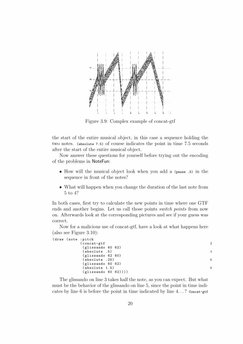
Figure 3.9: Complex example of concat-gtf

the start of the entire musical object, in this case a sequence holding thetwo notes. (absolute 7.5) of course indicates the point in time 7.5 secondsafter the start of the entire musical object.

Now answer these questions for yourself before trying out the encodingof the problems in NoteFun:

• How will the musical object look when you add a (pause .5) in thesequence in front of the notes?

• What will happen when you change the duration of the last note from5 to 4?

In both cases, first try to calculate the new points in time where one GTFends and another begins. Let us call those points switch points from nowon. Afterwards look at the corresponding pictures and see if your guess wascorrect.

Now for a malicious use of concat-gtf, have a look at what happens here(also see Figure 3.10):

(draw (note :pitch2(concat-gtf

(glissando 60 62)4(absolute .5)

(glissando 62 60)6(absolute .25)

(glissando 60 62)8(absolute 1.5)

(glissando 60 62))))

The glissando on line 3 takes half the note, as you can expect. But whatmust be the behavior of the glissando on line 5, since the point in time indi-cates by line 6 is before the point in time indicated by line 4. . . ? Concat-gtf

20

Figure 3.10: Complex example of concat-gtf

prints a warning on the screen saying: “Times being re-arranged!”Concat-gtfchecks if the successive switch points of its argument list are monotonouslyincreasing. Also it check whether all the switch points remain between thebounds of the start and end time of the note. If not, it changes the switchpoints so they will obey these two properties. In our last example concat-gtf

changes the switch point on line 6 into (absolute .5) (first property) and theswitch point on line 8 into (absolute 1) (second property). The result is thatthe glissando of line 5 will not appear since it has a time interval of exactly0 seconds. The glissando of line 5 will appear on the interval [.5, 1]. Theglissando of line 9 will not appear since it has a time interval of 0 seconds.In other words, the last example is equivalent to the following code:

(draw (note :pitch(concat-gtf(glissando 60 62)(absolute .5)(glissando 60 62))))

Try this out and see for your self.

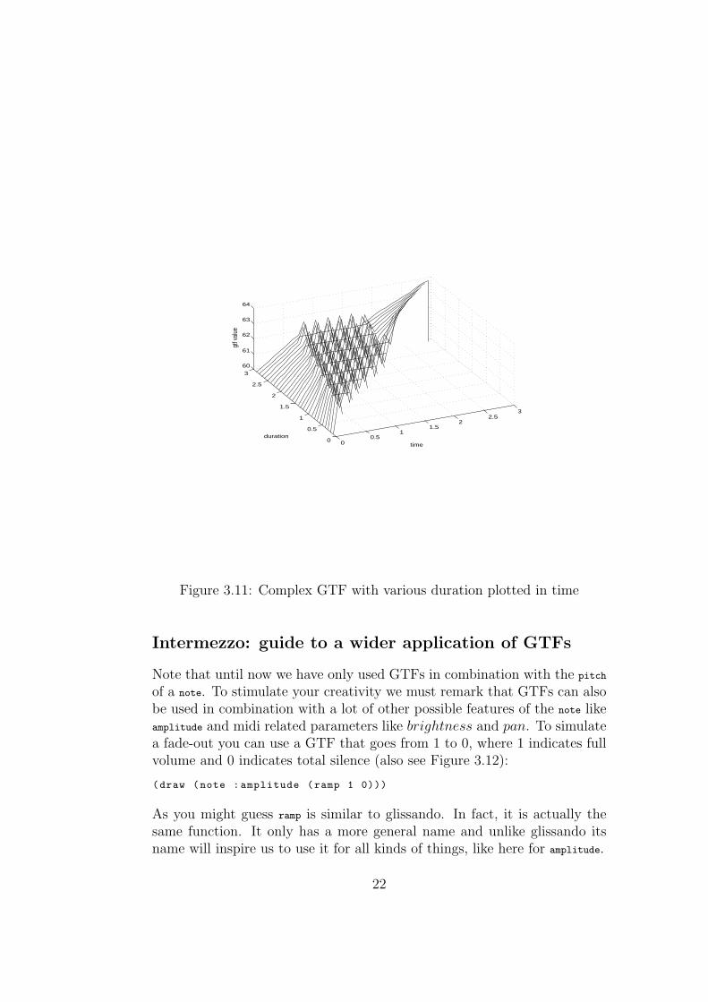
We conclude this subsection with a 3D graph of a complex GTF withduration from the interval [0, 3] plotted in time. See Figure 3.11. TheNoteFun code for this GTF is:

(concat-gtf(glissando 60 62)(proportional .25)(vibrato :around 62 :period .2)(relative 1.8)(glissando 62 64)(absolute 3.5)(glissando 64 60))

21

00.5

11.5

22.5

3

0

0.5

1

1.5

2

2.5

360

61

62

63

64

time

duration

gtf v

alue

Figure 3.11: Complex GTF with various duration plotted in time

Intermezzo: guide to a wider application of GTFs

Note that until now we have only used GTFs in combination with the pitch

of a note. To stimulate your creativity we must remark that GTFs can alsobe used in combination with a lot of other possible features of the note likeamplitude and midi related parameters like brightness and pan. To simulatea fade-out you can use a GTF that goes from 1 to 0, where 1 indicates fullvolume and 0 indicates total silence (also see Figure 3.12):

(draw (note :amplitude (ramp 1 0)))

As you might guess ramp is similar to glissando. In fact, it is actually thesame function. It only has a more general name and unlike glissando itsname will inspire us to use it for all kinds of things, like here for amplitude.

22

Figure 3.12: Note with a fade out

To make use of the midi controller related features of note, you can addthe synthesizer specific controller number and the range in which you wantto control it yourself. The code for the controllers that we have put in forour own synthesizer4 looks like this:

(add-midi-controller :pan 10 -1 0 1)(add-midi-controller :balance 8 0 .5 1)(add-midi-controller :timbre 71 0 .8 1)(add-midi-controller :brightness 74 0 .8 1)

You can make up any keyword your want for your specific controller. Thesyntax for add-midi-controller is

(add-midi-controllers<keyword ><midi control number ><minimal-value ><default-value ><maximum-value >)

For a panning from left to right within a note we could write:

(note :pan (ramp -1 1))

You can remove a midi controller by executing (remove-midi-controller <name>).For example, if we want to remove the controller for brightness, we write:(remove-midi-controller :brightness). To get a list of all currently availablemidi controllers you write: (show-midi-controllers).

Complex GTFs continued

Another tool for merging simple GTFs into a complex one is switch-gtf. Itworks slightly different than concat-gtf but has the same way of calling.

4A Yamaha MU90R

23

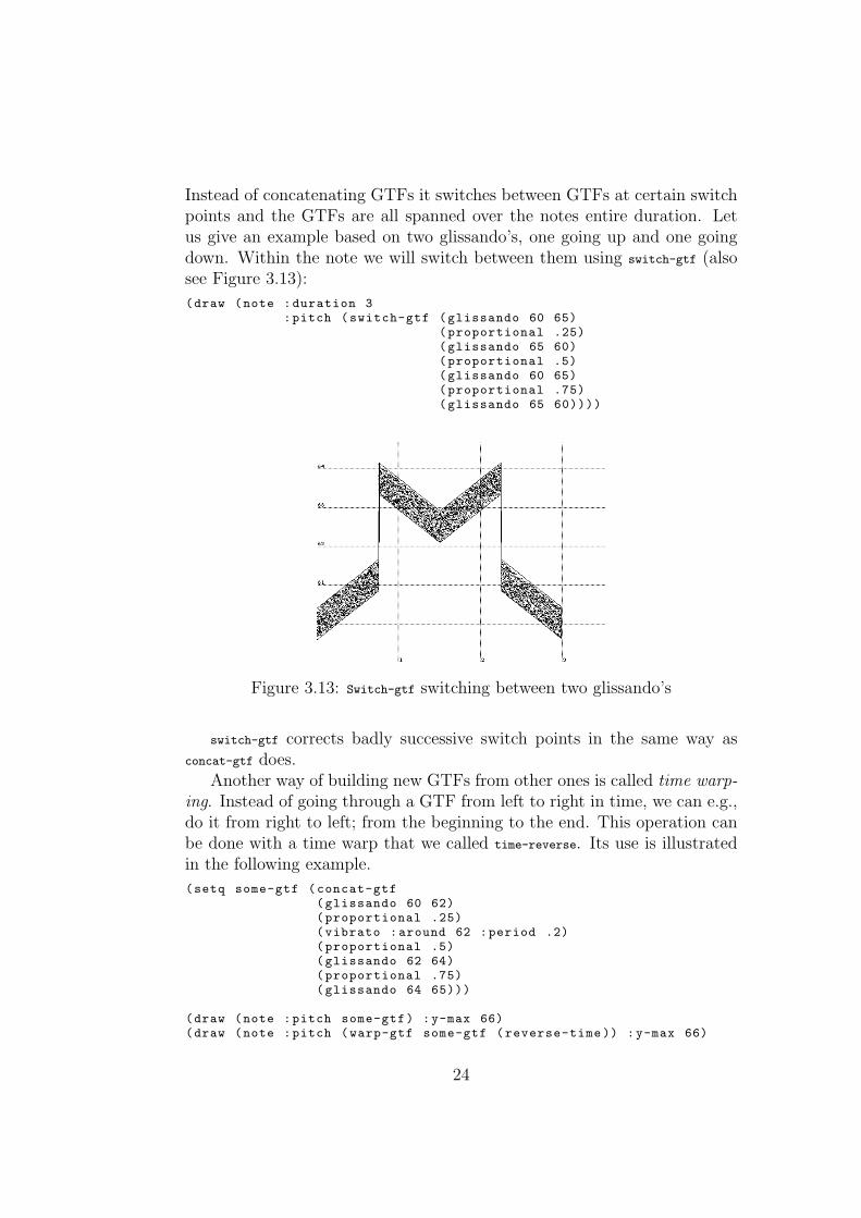
Instead of concatenating GTFs it switches between GTFs at certain switchpoints and the GTFs are all spanned over the notes entire duration. Letus give an example based on two glissando’s, one going up and one goingdown. Within the note we will switch between them using switch-gtf (alsosee Figure 3.13):

(draw (note :duration 3:pitch (switch-gtf (glissando 60 65)

(proportional .25)(glissando 65 60)(proportional .5)(glissando 60 65)(proportional .75)(glissando 65 60))))

Figure 3.13: Switch-gtf switching between two glissando’s

switch-gtf corrects badly successive switch points in the same way asconcat-gtf does.

Another way of building new GTFs from other ones is called time warp-ing. Instead of going through a GTF from left to right in time, we can e.g.,do it from right to left; from the beginning to the end. This operation canbe done with a time warp that we called time-reverse. Its use is illustratedin the following example.

(setq some-gtf (concat-gtf(glissando 60 62)(proportional .25)(vibrato :around 62 :period .2)(proportional .5)(glissando 62 64)(proportional .75)(glissando 64 65)))

(draw (note :pitch some-gtf) :y-max 66)(draw (note :pitch (warp-gtf some-gtf (reverse-time )) :y-max 66)

24

First we make a reference to a GTF to be able to write more readablecode. We use the name some-gtf as the reference name. Then we draw theresult of using some-gtf as a notes pitch (see Figure 3.14). Lastly we drawthe result of a transformed version of some-gtf by means of the time warptime-reverse (see Figure 3.15).

Figure 3.14: Note with some-gtf as a pitch

Figure 3.15: Note with some-gtf, transformed by a time warp, as a pitch

Another handy time warp is make-time-cyclic. Make-time-cyclic has oneargument indicating a point time within the duration of the note by meansof absolute, relative and proportional. I will show the use of make-time-cyclic

by means of an example (see Figure 3.16):

(draw (sim (note :duration 3:pitch (warp-gtf (glissando 62 65)

(make-time-cyclic (proportional .5))))

25

(note :duration 3:pitch (warp-gtf (glissando 60 62)

(make-time-cyclic (relative .5))))):y-max 66)

Figure 3.16: Note with a glissando which is transformed by a time warp, asa pitch

By now it might be clear how make-time-cyclic works. The point in timeindicated by the time switch is the period length which indicates after whatamount of time the GTF should start over again as if it were from the start.

There are more facilities that let us create GTFs out of other ones.One is called mix-gtf. By means of an example we will show its use (seeFigure 3.17):

(draw (note :duration 3 :pitch(mix-gtf(glissando 60 70)1(sine-gtf :period 2 :amplitude 1) 1))

:y-max 75)

The syntax in which you can use mix-gtf is: (mix-gtf [<gtf> <factor>]*).The factors in this expression can be real numbers or GTFs5. The result ofthis expression will be a gtf which is the weighted result of the succeedinggtfs and factors in the argument list. Our last example will be a gtf whichis the addition of a glissando from 60 to 70 and a sine with an amplitude of1 and a period of 2 seconds. Check Figure 3.17 if it looks like you expect.Because of the fact that we can either fill in a real number or a GTF as

5The notation we have used for the argument list must be read as a regular expressionin which <gtf> and <factor> can be arbitrary GTFs and numbers. The same holds forsuccessive examples in which this notation is used.

26

Figure 3.17: Example of mix-gtf

the factor, we are able to express things like: ”let the impact of a GTF runfrom 2 to 0 along with the duration of the note”. As follows:

(draw (note :duration 3 :pitch(mix-gtf (ramp 60 70)

1(sine-gtf :amplitude 1)(ramp 2 0)))

:y-max 75)

The first GTF is kept constant (the succesive factor is 1) but the secondGTF is multiplied by a ramp from 2 to 0. What we will expect is a rampwith a periodic deviation of which the amplitude will decrease as we gothrough the note in time. You can see the result in Figure 3.18.

Figure 3.18: Second example of mix-gtf

27

Another similar combinator of GTFs is interpolate-gtf. As its namesuggests, it interpolates between two GTFs. To make this clear let usinterpolate between a glissando and a vibrato:

Figure 3.19: Example of interpolate

(draw (note :duration 3 :pitch (interpolate-gtf (glissando 60 70) (vibrato ))):y-max 70)

The interpolation can be defined in terms of mix-gtf:(interpolate-gtf gtf1 gtf2) ≡ (mix-gtf gtf1 (ramp 1 0) gtf2 (ramp 0 1))

To give more elementary operations on GTFs we will introduce gtf+ andgtf*. After that we will introduce a more general function with which youcan make your own operation on GTFs.

A GTF that is the sum of multiple other GTFs can be made with gtf+

with the following syntax: (gtf+ [<gtf | number>]*). For example, we can adda glissando and another glissando so that they will compensate each other,resulting in a constant pitch:(note :pitch (gtf+ (glissando 30 40) (glissando 30 20)))

The result is just a note with a constant pitch of 60.The next example demonstrates the use of gtf* within the use of gtf+.

(draw (note :pitch (gtf+ 60 (gtf* (ramp 0 1) (sine-gtf :period .2)))))

The result is a note with a with-time-increasing periodic deviation frompitch 60 (see Figure 3.20).

If you require more operators on GTFs you can define them yourselfusing time-fun-compose. For example, if we would like to make the operatorfor division on GTFs we write:

(time-fun-compose #’/ [<gtf>]*)

More close to Lisp, a usable definition could be called gtf/ and would looklike this:

28

Figure 3.20: Example of gtf+ and gtf*

(defun gtf/ (gtf1 gtf2 &rest args)(apply #’time-fun-compose #’/ gtf1 gtf2 args))

We can use gtf/ from now on as demonstrated in the following example(see Figure 3.21):

(draw (note :duration 2:pitch (gtf+ 60 (gtf/ (sine-gtf :amplitude 5) (ramp 2 10)))))

Figure 3.21: Example of gtf/ embedded in a gtf+

GTFs created from mathematical functions

In this section we will describe how one can build a GTF based on a mathe-matical function, like the sine function. This way of building gives one moredegree of freedom of customizing your own GTFs as you will not be only

29

limited to the tools we provided before. Instead you can come up with anymathematical function you wish. You can specify how it should behave un-der transformation. Like we saw with the glissando, some functions shouldtransform in a proportionally stretching way. Other functions, similar tothe vibrato, should not be stretched. We call the creation of a GTF out ofa mathematical function lifting.

A mathematical equivalent of the glissando might be a linear function,like (lambda(x) x). Suppose we want to have a mathematical function thatcorresponds to a glissando from 60 to 70. Note that we do not know the du-ration of the note, to which the function will be applied, since it can be anypositive real number. For now we will just choose a function that goes from60 to 70 in an interval of 1 second: (setq linfunc #’(lambda(x) (+ 60 (* 10 x))))

Now look at the following example (see Figure3.22):

(draw (note :duration 2 :pitch (lift linfunc (proportional-lift 0 1))):y-max 72)

Figure 3.22: Example of a mathematical function lifted proportionally

What does (lift linfunc (proportional-lift 0 1)) mean? Informally it means,select the function linfunc on the interval [0, 1] and stretch it according tothe duration of a note.More general, the syntax for lift is: (lift <mathematical function> <lift-function>).proportional-lift is a lift function that selects an interval out of a mathemati-cal function. Try to modify the duration of the note in the last example andsee that its pitch still runs from 60 to 70. This is how we want a glissandoto behave under transformation.

Another lift function is relative-lift. It does not help us to stretch aselection out of a function but it lets us express something else. Let us tryit out as a variation on our last example.

30

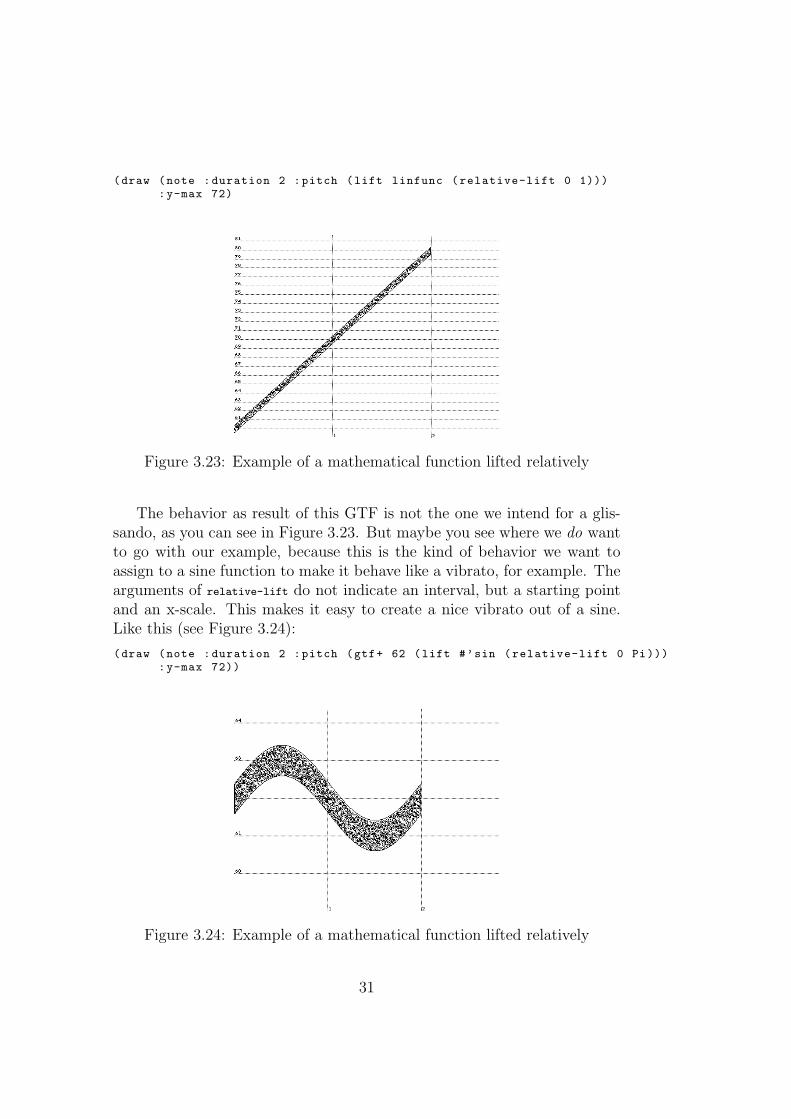
(draw (note :duration 2 :pitch (lift linfunc (relative-lift 0 1))):y-max 72)

Figure 3.23: Example of a mathematical function lifted relatively

The behavior as result of this GTF is not the one we intend for a glis-sando, as you can see in Figure 3.23. But maybe you see where we do wantto go with our example, because this is the kind of behavior we want toassign to a sine function to make it behave like a vibrato, for example. Thearguments of relative-lift do not indicate an interval, but a starting pointand an x-scale. This makes it easy to create a nice vibrato out of a sine.Like this (see Figure 3.24):

(draw (note :duration 2 :pitch (gtf+ 62 (lift #’sin (relative-lift 0 Pi))):y-max 72))

Figure 3.24: Example of a mathematical function lifted relatively

31

Now try to modify the duration of the note from the last example againand see what happens! Is it the behavior you desire from a vibrato?

The last lift function for simple functions we will discuss is absolute-lift.It is different from relative-lift in that it does not see the notes start as thestarting point (time = 0) for the GTF, but it uses the start of the wholemusical object as the starting point of the GTF. Let us illustrate this witha vibrato that is lifted using absolute-lift and that is used over a group ofnotes.

(draw (seq (sim(seq (note :duration 2 :pitch (gtf+ 60 lifted-sine ))

(note :duration 1 :pitch (gtf+ 57 lifted-sine )))(seq (note :pitch (gtf+ 63 lifted-sine ))

(note :pitch (gtf+ 64 lifted-sine ))))(note :duration 2 :pitch (gtf+ 65 lifted-sine )))

:y-min 55:y-max 70)

Figure 3.25: A group of notes, all with the same lifted sine function by useof absolute-lift

Because the starting point of the whole group of notes is taken as time =0 you can see the sine wave continuously running through all notes, as if itdoes not know where one note ends and another begins.

Lifting tables

Another method of creating GTFs is by means of tables. You can specifya table with key and value pairs and lift it as if it were a mathematicalfunction. An example is given below.

(setq my-table ’((0.0 60)(.1 61.4)

32

(.2 62.3)(.3 61.2)(.7 65)(1 60)))

With the help of table-fun we can make a simple function out of a table:(setq tablefunction (table-fun my-table ))

Since tablefunction now is a simple function, we can use it in the sameway as any other simple function. Hence we can lift it with the same con-structions as demonstrated in the previous subsection. The function is madeby a lineair interpolation between the values of the table, as demonstratedin the following code (see Figure 3.26):(draw (seq (note :duration 2

:pitch (lift tablefunction (proportional-lift 0 .5)))(note :duration 2

:pitch (lift tablefunction (relative-lift 0 .5)))):y-max 66)

Figure 3.26: Example of a table, converted to a simple function and lifted

Creation of GTFs by writing your own Lisp code

In this last subsection on the creation of GTFs we will address you to writeyour own Lisp code as a means of creating your own GTFs. In order to dothat we have to go into details of how a GTF is built up. We will do this,like you are used to in this tutorial, by means of example. First we willshow how an existing GTF is built up. After that we will write a new onefrom scratch.

Do you remember the glissando GTF from all the previous examples?As we already said it is the same function as the ramp function. Here is itsencoding in Lisp:

33

(defun ramp (from to)2(gtf (start duration)

(tf(time)4(let (( progress (/ (- time start) duration )))

(+ from (* progress (- to from )))))))

In general a GTF is built up using the construction

(gtf (start duration)(...(tf (time) (...))...)

ramp returns a function of the type R+ → R+ → (R+ → R+). Theconstructions gtf and tf work like normal functional abstraction. Theyare adapted versions of Lisps lambda, enhanced for our purpose here. gtf

creates a function of the type R+ → R+ → (R+ → R+) and tf creates afuntion of type R+ → R+. A GTF makes use of three important variablestime, start and duration. The variable time indicates the time counted fromthe start of an entire musical object; start indicates the time at which thenote in which the GTF will be used will begin; duration represents the timeinterval on which a note will be played. The dots on the second line of thegeneral code are intended to consist of calculations with start and duration.Calculations that involve also time can only occur inside the tf construction.This two layer way of building a GTF is chosen because of efficiency reasonswhich we will not have to discuss at this stage. Look at section 6.3 for moreon this. Because all of the calculations that we need in ramp involve time,they have to occur inside the tf.

Now let us look how ramp works. On line 4 of its code an expressionwith time, start and duration is bound to progress. If we look closer to theexpression we see that it indicates the fraction of the duration that hasalready passed: ”current time minus start time” divided by ”total durationof the note”. At the very start of the note, progress will have value 0. Atthe very end of the note ”time minus start” will equal duration and thereforeprogress will have the value of 1. Now, with (ramp <from> <to>) we want tohave a GTF that is a linear function from <from> to <to> on the interval[start,start+duration]. Note that the expression(+ from (* progress (- to from))))))) returns the right value on each point oftime on in the interval.

Now that we have seen the implementation of ramp it may inspire us tomake a different GTF. Wouldn’t it be funny to make a GTF that givesrandom values from a certain range? In Lisp (random <n>) returns a randomfloating point number from the range [0, n[ (n self is excluded) when n is afloating point number. Hence (random 1.0) returns a floating point numberbetween 0 and 1. The Lisp expression (+ min (* (- max min) (random 1.0)))

34

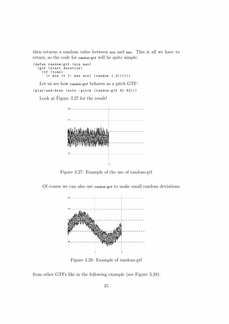
then returns a random value between min and max. This is all we have toreturn, so the code for random-gtf will be quite simple:

(defun random-gtf (min max)(gtf (start duration)

(tf (time)(+ min (* (- max min) (random 1.0))))))

Let us see how random-gtf behaves as a pitch GTF:

(play-and-draw (note :pitch (random-gtf 61 62)))

Look at Figure 3.27 for the result!

Figure 3.27: Example of the use of random-gtf

Of course we can also use random-gtf to make small random deviations

Figure 3.28: Example of random-gtf

from other GTFs like in the following example (see Figure 3.28):

35

(draw (note :duration 2:pitch (gtf+ (vibrato :around 61)

(random-gtf 0 .5))))

.

Case study: ADSR

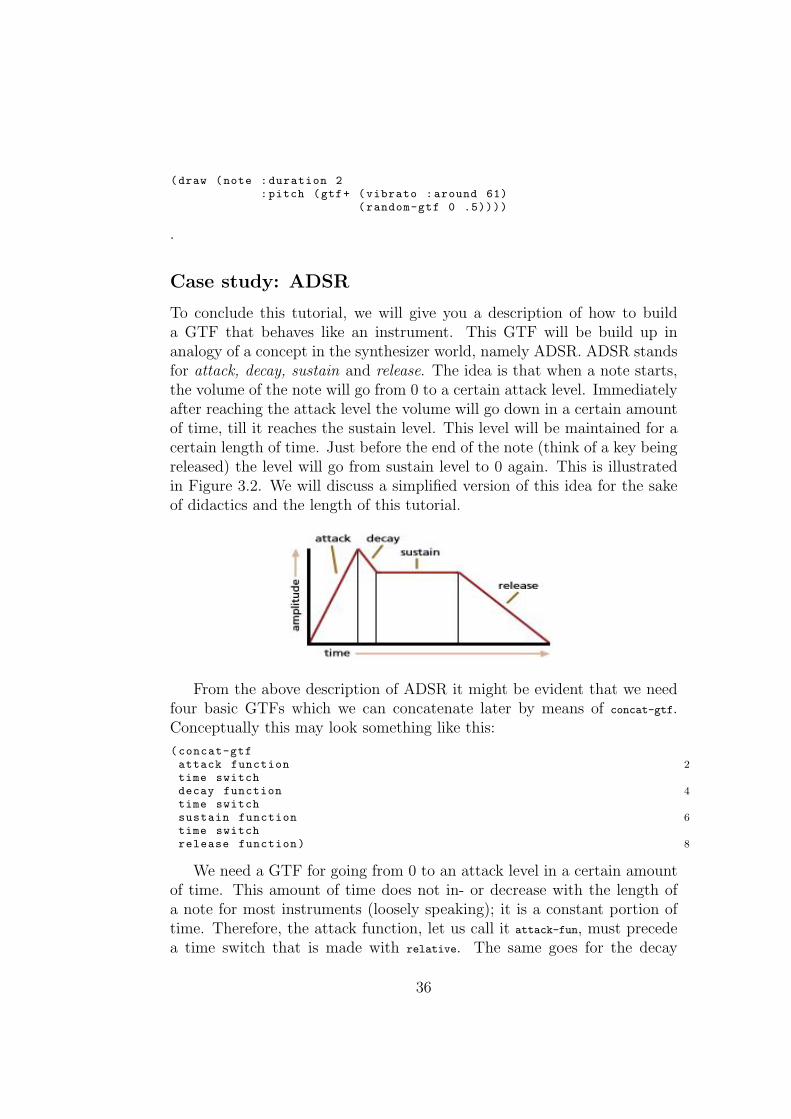
To conclude this tutorial, we will give you a description of how to builda GTF that behaves like an instrument. This GTF will be build up inanalogy of a concept in the synthesizer world, namely ADSR. ADSR standsfor attack, decay, sustain and release. The idea is that when a note starts,the volume of the note will go from 0 to a certain attack level. Immediatelyafter reaching the attack level the volume will go down in a certain amountof time, till it reaches the sustain level. This level will be maintained for acertain length of time. Just before the end of the note (think of a key beingreleased) the level will go from sustain level to 0 again. This is illustratedin Figure 3.2. We will discuss a simplified version of this idea for the sakeof didactics and the length of this tutorial.

From the above description of ADSR it might be evident that we needfour basic GTFs which we can concatenate later by means of concat-gtf.Conceptually this may look something like this:

(concat-gtf2attack function

time switch4decay function

time switch6sustain function

time switch8release function)

We need a GTF for going from 0 to an attack level in a certain amountof time. This amount of time does not in- or decrease with the length ofa note for most instruments (loosely speaking); it is a constant portion oftime. Therefore, the attack function, let us call it attack-fun, must precedea time switch that is made with relative. The same goes for the decay

36

function, which we will call decay-fun and its succeeding time switch. Thesustain, named sustain-fun, does depend on the duration of the note. Theportion of time needed for the release, let us call it release − fun, fromsustain level to 0 is again a constant portion. With this information we canmake the concept a bit more concrete:

(concat-gtf2attack-fun

(relative ...)4decay-fun

(relative ...)6sustain-fun

(relative ‘end time minus ’ ...)8release-fun)

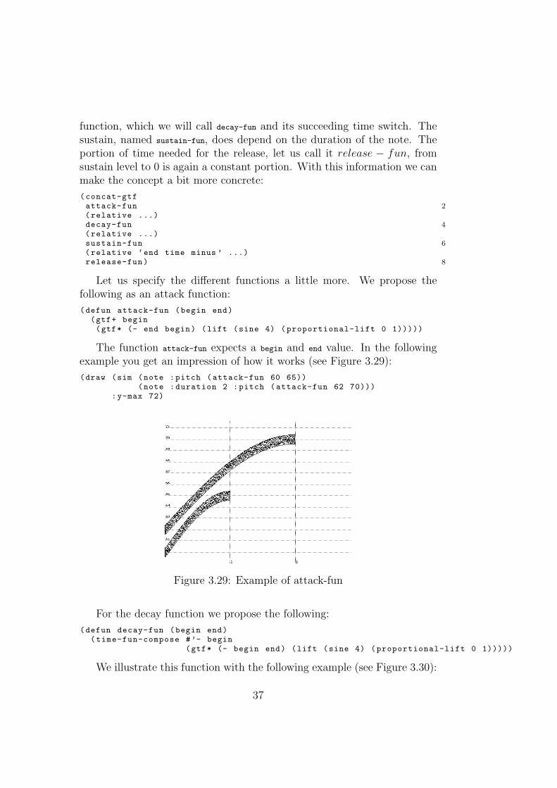
Let us specify the different functions a little more. We propose thefollowing as an attack function:

(defun attack-fun (begin end)(gtf+ begin(gtf* (- end begin) (lift (sine 4) (proportional-lift 0 1)))))

The function attack-fun expects a begin and end value. In the followingexample you get an impression of how it works (see Figure 3.29):

(draw (sim (note :pitch (attack-fun 60 65))(note :duration 2 :pitch (attack-fun 62 70)))

:y-max 72)

Figure 3.29: Example of attack-fun

For the decay function we propose the following:

(defun decay-fun (begin end)(time-fun-compose #’- begin

(gtf* (- begin end) (lift (sine 4) (proportional-lift 0 1)))))

We illustrate this function with the following example (see Figure 3.30):

37

(draw (sim (note :pitch (decay-fun 65 62))(note :duration 2 :pitch (attack-fun 70 64)))

:y-max 72)

Figure 3.30: Example of decay-fun

The sustain function can be really simple. It just has to remain constantat a certain level:(defun sustain-fun (volume)

(gtf (start duration)(tf (time)volume )))

As a release function we can take the same function as the decay func-tion:(defun release-fun (begin end)

(decay-fun begin end))

Finally we are ready to try out our ADSR. We build a function aroundit in which you can specify the different levels and time intervals.(defun adsr (attack-time decay-time release-time attack-level sustain-level)

2(let (( att-time (relative attack-time ))(dec-time (relative (+ attack-time decay-time )))

4(rel-time (fun-funcall #’- #’end-time release-time )))(concat-gtf (attack-fun 0 attack-level)

6att-time(decay-fun attack-level sustain-level)

8dec-time(sustain-fun sustain-level)

10rel-time(release-fun sustain-level 0)

12)))

The expression (fun-funcall #’- #’end-time release-time) evaluates to theend time of the note minus the time interval indicated by release-time. Be-cause end-time and release-tim are not normal numbers (actually they arefunctions) we have to use fun-funcall in this case.

38

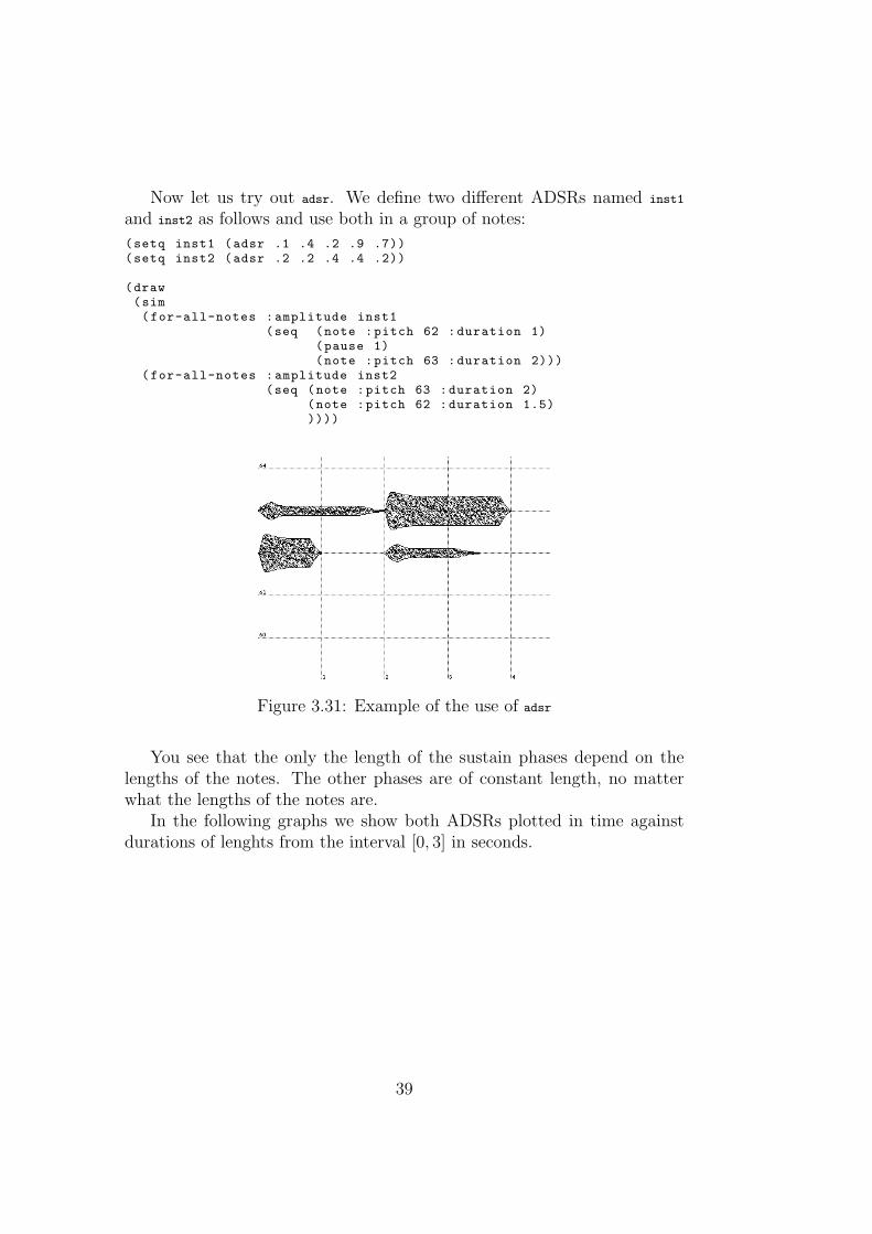
Now let us try out adsr. We define two different ADSRs named inst1

and inst2 as follows and use both in a group of notes:

(setq inst1 (adsr .1 .4 .2 .9 .7))(setq inst2 (adsr .2 .2 .4 .4 .2))

(draw(sim(for-all-notes :amplitude inst1

(seq (note :pitch 62 :duration 1)(pause 1)(note :pitch 63 :duration 2)))

(for-all-notes :amplitude inst2(seq (note :pitch 63 :duration 2)

(note :pitch 62 :duration 1.5)))))

Figure 3.31: Example of the use of adsr

You see that the only the length of the sustain phases depend on thelengths of the notes. The other phases are of constant length, no matterwhat the lengths of the notes are.

In the following graphs we show both ADSRs plotted in time againstdurations of lenghts from the interval [0, 3] in seconds.

39

00.5

11.5

22.5

3

0

0.5

1

1.5

2

2.5

30

0.2

0.4

0.6

0.8

1

time

duration

gtf v

alue

Figure 3.32: The GTF (adsr .1 .4 .2 .9 .7) plotted for durations from 0 to3 seconds

40

0 0.5 1 1.5 2 2.5 30

0.5

1

1.5

2

2.5

3

0

0.1

0.2

0.3

0.4

time

gtf v

alue

duration

Figure 3.33: The GTF (adsr .2 .2 .4 .4 .2) plotted for durations from 0 to3 seconds

41

Chapter 4

Overview of NoteFun’sfunctions

In this chapter we give an overview of the functions that a NoteFun usercan use to compose music. Each function name will be given, followed bythe page number where the use of the function is explained. Possibly someadditional comments are given. For all the examples of the use of thesefunctions we redirect you to chapter 3.

4.1 Construction of musical objects

This section is an overview of the functions that allow you to build musicalobjects.

pause The most simple musical object is a pause. More information onpage number 10.

note The most basic musical object next to pause is a note. It is describedon page number 10 and further.

:program With this aspect of a note one can choose the program numbershould be used when the note is played on a synthesizer. More informationon page 12.

:channel With this aspect of a note one can choose the channel numberon which a note should be played. More information on page 12.

42

for-all-notes This is a construct to assign an aspect to a group of notes.More information on page ??.

seq This function is used to make sequences of musical objects and isexplained on page 11.

sim This function is used to make simultaneous compositions of musicalobjects and is explained on page 11.

trans With trans one can transpose an entire musical object. More infor-mation can be found on page 12.

stretch With stretch one can stretch an entire musical object. More in-formation can be found on page 13.

4.2 Construction of GTFs

glissando This is a predefined GTF. More information on page 13.

vibrato This is a predefined GTF. More information on page 14.

ramp This is a predefined GTF. More information on page 22.

proportional This functions allows to express a point in time as a pro-portion of a note’s duration. More information on pageref 18.

relative This functions allows to express a point in time as relative to thenote’s start. More information on pageref 19.

absolute This functions allows to express an absolute point in time. Moreinformation on pageref 19.

concat-gtf This functions allows to concatenate multiple GTFs as de-scribed on page 17.

switch-gtf This functions allows to combine and switch between multipleGTFs as described on page 23.

43

mix-gtf A function to mix GTFs as described on page 26.

interpolate-gtf A function to interpolate between GTFs, described onpage 27.

gtf+ A function to sum GTFs, described on page 28.

gtf* A function to multiply GTFs, described on page 28.

time-fun-compose A function to compose GTFs using mathematicaloperators as described on page 28.

lift A function to create a GTF from a mathematical function, describedon page 30.

proportional-lift A lift function used within lift as described on page30.

relative-lift A lift function used within lift as described on page 30.

absolute-lift A lift function used within lift as described on page 32.

table-fun A function that creates a function from a table, described onpage 33.

gtf The construction to create a GTF, as documented on page 34.

tf The construction that is used within gtf to create a GTF, as docu-mented on page 34.

time-reverse A time warp, described on page 24.

make-time-cyclic A time warp, described on page 25.

4.3 Mediate musical objects

Show musical objects

draw This function shows a graphical representation of a musical object.

44

Play musical objects

play (musical-object)

The musical object will be translated into a midi sequence which will beinterpreted by a connected midi synthesizer. A more detailed descriptioncan be found on page 12.

add-midi-controller Notes: the name of a midi controller, indicatedby name should have the form of a Lisp keyword, preceded by a colon :.Optionally a range indicating the minimum, default and maximum of acontroller can be given by giving three integer values min, def and max. Byspecifying a midi specific controller with e.g., the name :brightness it can beused in a note similar to a normal property of a note, like :pitch. A detailedexample can be found on page 22.

remove-midi-controller With this function a synthesizer specific midicontroller can be removed from the controller list. More information canbe found page 23.

show-midi-controllers With this function the controller list can be printedon the screen.

45

Chapter 5

Other programming languagescompared to Lisp

5.1 Introduction

Only less than four months ago I started to learn to program and thinkin Lisp. It was an educative time in which I grew enthusiastic about Lisp.But at times it was also a frustrating time in which I felt negative towardsthe language. In what follows I will try to stipulate how Lisp relates toother programming languages. I will try to give an objective-as-possibleoverview of the pro’s and cons of Lisp in relation to other programminglanguages and their usages. I hope it will be clear that Lisp is a languagethat deserves serious consideration as language of choice in both softwareengineering and Artificial Intelligence research. Also I hope to clear upsome myths around Lisp and declarative languages in general. In chapter 6we will see a practical illustration of the characteristics of Lisp within theNoteFun project.

5.2 Why Lisp?

During the past few months I asked a lot of people who are active in the fieldof computer science why they preferred their language of choice over others.Together with my own knowledge and experience, certain characteristics ofLisp and the other languages became evident and need to be mentioned inthis section. By means of these characteristics I will try to give an answer tothe question: ”Why Lisp?” In Norvig (1992) page ix, I found a summary ofsome important aspects of ”Why Lisp?” These three more or less categorizethe issues I would like to discuss. First I will give Norvigs three arguments.

46

Later I will discuss each of them in more detail and I will contrast themwith possible counter-arguments. The three arguments Norvig names arelisted here:

1. Lisp is a very popular language for AI programming. If you are goingto learn a language, it might as well be one with a growing litera-ture, rather than a language which is not widely used anymore and isdoomed to be one of dead tongue.

2. Lisp makes it easy to capture generalizations in defining new objects.In particular, Norvig says, Lisp provides the means to define newlanguages that are problem specific. This is handy in AI applicationswhich often manipulate complex information which is best representedin some novel form.

3. Lisp makes it very easy to develop a working program fast. Lispprograms are concise and are uncluttered by low-level detail.

Ad 1

I think this is a good argument for picking a language, but it might not bethe strongest one to defend Lisp. Until a few months ago I rarely ever heardabout Lisp. A class about parallel garbage collection was an exception inthis case, but even there I did not see a fragment of Lisp code. Lisp is apopular language in the AI world, but particularly in the United States.Most of the people in Europe, where I happen to live, who I spoke toand did know about Lisp, were kind of skeptical about Lisp similar in theway people are skeptical about the artificial human language Esperantonowadays. Where does this skepticism come from? During the past fewmonths I got the feeling that, like Esperanto, Lisp has a hidden value thatpeople must have forgotten over the past few decades or simply have notdiscovered yet.

Parentheses scary?

The reason of this may lay in the fact that at first glance both languagesmake a weird impression; they take some time to get used to, both inreading, thinking and writing. For example, a often-heard critic on theLisp syntax is: ”Too much parentheses!” When I think back of my historyin programming in other languages, I think the parentheses in Lisp are nomore a burden than the curly bracket pairs and semicolons we know from

47

e.g., Pascal and Java. Especially with a good editor1 the parentheses andindentation do not form a big problem anymore.

Familiarity

One other reason could be that programmers nowadays more or less takeconfidence in only one programming style: either imperative, object ori-ented (or a mix of the latter two) or declarative (logical and functional).This could be simply out of lack of knowledge of other possible styles. Alsoit could come from the culture in which the programmer was educated.Stubborn propaganda sometimes is made for one specific paradigm whichcan have a huge impact on how the programmer thinks about other lan-guages. I see this not only at universities, but also at companies wheresometimes tradition is the main factor in choosing a language.

Hybrid style: good or bad?

Another reason for suspicion is that Lisp combines a lot of paradigms. Howcan a language that is a mix of paradigms be a clean and concise language?In this respect it resembles Esperanto too, but in a different way. Esperantois more or less a compromise between existing european natural languages.Lisp, on the other hand, is not a compromise between existing programminglanguages. It truly incorporates the full power of imperative, functional andobject oriented programming. This should not be something to be scared offby. It should be considered as a challenge to travel beyond the boundariesof one paradigm!

Specific or general purpose?

A myth that still lives among imperative programmers is that declarativelanguages are problem dedicated languages and that their language is oneof general purpose. Clearly this is not the case. The imperative languagesreflect the inner state of a computer system. They do not reflect the wayhow we would mathematically, logically and intuitively describe a prob-lem. Other than doing that, an imperative program consists mainly outof (possibly parallel) sequences of instructions. Some, if not most of theseinstructions describe how variables should be updated in the next iterationof the program. Most of these imperative languages are nothing more thana high level description of what the resulting machine code should look like.

1Like the editor that goes with MCL: Fred

48

This is not what I call a general purpose language because it has specializedtask: to make machine code more readable and writable.

Side effects and reasoning about programs

An ideal that comes from the declarative programmer’s society is that codeshould be clean. An interpretation of this statement is that by means ofthe code one should be able to reason about the results of the programor one should be able to prove the correct workings of the program bymeans of the code only. A consequence of this is that code should be sideeffect free. Any computation should not change the global state of othercomputations. Programming languages that do quite the opposite are theimperative languages described above. Therefore they are not regarded assuitable for e.g., explaining algorithms and proving their correctness. Oftenthe syntax of an imaginary pseudo language or a purely declarative languageis used for this purpose. Sometimes declarative languages therefore also arecalled executable specification languages. Lisp combines both side-effect-free and state-changing programming. For this reason Lisp might not beregarded as a pure and clean language by theoreticists and therefore will beput aside by them. An objection to this argument can be that a language iseither at the same time really side-effect-free and useless or not really side-effect-free. Please note that reading from a file or keyboard and writingto a file or screen are state-changing operations. If a running programwould totally have no state-changing properties, how would we ever noticethat the program actually works correctly? There would be nothing in theworld changed for us to be remarked. Another objection is that Lisp can beused in the same side-effect-free way of programming like pure functionallanguages. In this case, one simply must not make use of state-changingconstructions.

Survival of the fittest?

Norvig points out that Lisp is an old language. Indeed it is. Its originslay in the thinking of McCarthy, a Princeton student of Alonzo Church.McCarthy invented Lisp in 1958. Many people think this language hassurvived many others because of its flexible approach to self-reference andextension. In Lisp data and programs reside on the same level: both areobjects built as a list, the key structure in Lisp. Therefore both can betreated as data and programs. This makes the alteration of programs withinprograms possible. This approach is widely exploited within macro’s. Amacro is used to generate Lisp program code, possibly by alteration of a

49

program passed as an argument. This might be one of the most importantreasons why Lisp has made it until this day. By means of macro’s otherprogramming paradigms could be incorporated within Lisp. This makesLisp distinct from other existing programming languages, both imperativeand declarative.

Ad 2

Dynamical typing and regularity in representation

This characteristic of Lisp is something that is handy in not only AI appli-cations but, I think, everywhere a program is being designed and developed.I have experienced this beneficial property of Lisp throughout the NoteFunproject. As no other language I worked in previously, Lisp allowed me to beflexible and generalizing over data and even programs by means of macro’s.One of the reasons of this flexible way of working may be that Lisp is adynamical typed language. Another may be that all data and programsrepresented in Lisp are represented by a list. Dynamical typing and syntaxregularity make it possible to write very general operations on data andprograms which can be used in a wide variety of situation. This is unlikeI am used to in statical typed languages where every data type must beaccompanied by a set of functions to create, manipulate and destroy them,in order to work with them in a satisfying way. In these languages sometime can be saved by means of overloading and generic programming, butstill work has to be done explicitly for every type.

Ad 3

Code esthetics

In my opinion Lisp code is uncluttered by low-level detail, although notoptimally. There still is some cluttering which probably scares people offhere and there. I will give two examples that show how Lisp code is not asuncluttered as possible.

(setq func #’(lambda(x)(* 2 x)))(funcall func 2)

On the first line we see an assignment of an anonymous function, aso called lambda expression, to the name func. In Lisp we have to makeuse of quotations to separate between data and programs. With a ’ weindicate that a list is meant as data and should not be evaluated. The# adds an indication that the object we are quoting is a function. Thisis something that might be regarded as ugly and cluttered syntax. On

50

line 2 we try to apply the function to an argument. In this case we haveto use funcall. If the syntax would be clean I would at least expect thatwe could do something like this: (func 4). This is supported in the Lispvariant called Scheme but not in Common Lisp. This is something I wouldlike to see changed to the Lisp syntax, although I do not know what newproblems it might introduce. Lisp programs, as Norvig states, are ofteneasy to read and do not have many details that do not directly relate to theprogramming problem. But there are some other languages of which thesyntax is more beautiful in my opinion. I will draw a comparison with thefunctional programming language Amanda here:

In Lisp, a new function that is constructed from a function by applyingit twice, can be made as follows:

(defun double (fun)#’(lambda(arglist)(funcall fun (funcall fun arglist ))))

To create and use a function that is twice the application of the functionf(x) = x2 we can write the following:

(funcall (double #’(lambda(x) (* x x))) 2)

The result is 16.In Amanda we could do all the same with:

double f = args -> f (f args)double (x- >x^2) 2

Of course the result is also 16. It is to you to decide, but I think Amandalooks better in this case. Norvig is right that Lisp code is uncluttered andwithout low-level details, compared to languages like C, Pascal, Java. ButI think the comparison cannot be drawn towards languages like Amanda,Haskell and Clean.

Debugging

As mentioned in the previous subsection the dynamical typing in Lisp bringsan advantage in favor of rapid prototyping. But alas, it also comes with adisadvantage: it can make debugging much more harder. Error messagesgenerated as a result from a programming mistake can occur at the bottomof execution. Therefore error messages sometimes do not get us quickly tothe ”place of crime” but can take us into a long and frustrating crusade.

Interactiveness

A last issue, this time in favor of the third argument, I would like to pointout is that Lisp is an interactive language. By means of the REPL, the

51

Read-Evaluate-Print-Loop, code can be tested immediately. This can becontrasted against the way of working in other languages in which one oftenhas to build an environment for reading and printing and compile completeprograms in order to test. The interactive property of a Lisp environmentspeeds up the way of working considerably. During my internship I used aninteractive editor in which one can select a fragment of code which can beexecuted after pressing a certain key. This is even a better alternative fora prompt at which one can insert code for execution and it helps to workeven faster.

5.3 Conclusions

In this chapter I contrasted Lisp with other languages. Three claims aboutwhy Lisp ought to be a programming language of choice were discussed. Inthe discussion several characteristics of Lisp arose:

• Lisp is not as weird as it may seem: it is merely a question of famil-iarity.

• Lisp combines programming paradigms

• Lisp is a general purpose language

• Lisp can be used as a side-effect-free language

• By means of macro’s Lisp survived many languages and can be ac-customed to your programming style and paradigm

• In Lisp, both data and programs are represented in the same way.Regularity (and dynamical typing) provides us with a means to makestrong generalizations.

• Lisp syntax is uncluttered and concise. Compared to a lot of (im-perative) languages it is better to read, although there exist otherlanguages that read even better.

• Lisp is an interactive programming language.

52

Chapter 6

Design and Implementation

In this chapter we will discuss some interesting cases from the process ofdesigning and implementing NoteFun. During this chapter we assume thereader has a basic knowledge of functional programming and hopefully Lispin specific. We will discuss some items that we found useful to demonstratehere for a number of reasons. One of the reasons is to show what importantdesign decisions have been made. Another reason is to show where and whythe characteristics of Lisp played an important role.

6.1 Notes on functional programming style

During the design and implementation of NoteFun we often discovered theusefulness of the functional programming paradigm. Having functions avail-able as first class citizens often led to a better generalized design. To give aconcrete example of this we will describe how we used the functional stylein the design of concat-gtf.

When we first toyed with the idea of concat-gtf we constructed a functionthat had an argument list that consisted of GTFs and numbers expressingpoints in time. For example users could do something similar to this:

(concat-gtf (ramp 0 1) .1 (ramp 1 0) 3 (ramp 0 1))

We thought it would be handy if users could express points in timerelative to the start of a note, as a proportion of the note’s duration or justas an absolute point in time. Somehow these numbers had to be combinedwith an indication of what kind of time was meant. Then the idea arose touse a more functional way of expressing points in time. We introduced thefollowing way the could be used in any function needing an argument thatexpresses a point in time:

• Absolute points in time n can be expressed like: (absolute n)

53

• Points in time n relative to the beginning of a note can be expressedlike: (relative n)

• Points in time n as a proportion of the note’s duration can be ex-pressed like: (proportional n)

Now users had to be able to do things like:

(concat-gtf (ramp 0 1) (proportional .1) (ramp 1 0) (absolute 3) (ramp 0 1))

as is the case in our definitive implementation. Implementation-wisethese expressions of time are functions that themselves have anonymousfunctions as a result. Let us take proportional as an example here:

(defun proportional (proportion)(time-expr (start duration)

(+ start (* proportion duration ))))

The construction time-expr is equivalent to Lisp’s lambda with some ad-ditional error catching. The result of proportional thus is an anonymousfunction of two arguments, start and duration. When called with the startand duration of a note, this anonymous function returns a point in timebetween the start and end of the note, according to the proportion that isgiven as a numerical argument to proportional.

Because absolute, relative and proportional all have anonymous functionsas a result of the same arguments and results, these anonymous functionscan be treated alike by concat-gtf. The way of specifying a point in timeis directly associated with the corresponding way of calculating the pointin time, because the way of specifying is a Lisp expression itself. Thecalculation is delayed, by means of creating anonymous functions, until acertain moment on which the real start and duration of a note are known.This way of programming is only possible in a functional programminglanguage, a language in which functions are first class data objects: theycan serve as arguments and results of other functions.

6.2 Extending the language by use of

macro’s

One of the useful characteristics of Lisp is that it is an extensible language.Unlike languages like Pascal and Java, Lisp can be augmented with languageconstructions. A simple example is the while loop that is not standardlyincluded in Lisp. A macro for adding it to the language is given below(taken from Norvig (1992), page 67):

54

(defmacro while (test &rest body)(list* ’loop

(list ’unless test ’(return nil))body))

We will not go into a deep level of detail here. For a full explanationof this macro and macro’s in general please read the section about macro’sin Norvig (1992), pages 66 to 68. What happens when we use this macrowith a test, a piece of code that results in to t or nil, and a body, a blockof executable Lisp code, is that the result is Lisp code that is understoodin terms of normal Lisp code. The following translation takes place:

(while <test> <body>) → (loop (unless <test> (return nil)) <body>) This ex-plains the back-quotes you see in the code. The back-quotes indicate thatthe word following it should be literally generated. This also explains whywe don’t see a preceding back-quote before test and body, namely becausethey are anonymous pieces of Lisp code.

An example of the use of while:

(let ((n 0))(while (< n 5)

(progn(print n)(incf n))))

and the result:

01234NIL

With macroexpand-1 we can see the macro-expansion of a macro, which isthe code that is generated as a result of the use of a macro. Applied to ourexample above,

(macroexpand-1 ’(while (< n 5)(progn

(print n)(incf n))))

gives

(LOOP(UNLESS (< N 5)

(RETURN NIL))(PROGN (PRINT N) (INCF N)))

One can imagine that the while construction is a very handy addition tothe language. During my internship I have written a macro that is some-what more complex but turned out to be very useful in different situations.

55

It is an iterative construction very similar to Lisp’s dolist. Instead of it-erating over every single element in a list, our macro makes it possible toiterate over sets of neighboring elements in a list, which we call a window.The language construction is called do-window-list and it is demonstrated inthe examples below.

For the sake of the example we will first define the Fibonacci sequence:

(defun fib (n)(cond (( equalp n 1) 1)

(( equalp n 2) 1)(t (+ (fib (- n 1)) (fib (- n 2))))))

(defun fibonacci (n)(cond (( equalp n 1) (list 1))

(t (append (fibonacci (- n 1)) (list (fib n))))))

The function fibonacci returns the first n elements of the Fibonacci se-quence, where n is the argument of fibonacci.

(fibonacci 10)

results in:

(1 1 2 3 5 8 13 21 34 55)

Suppose that we would want to have the product of every three suc-ceeding numbers in this list. With do-window-list this can be easily done:

(do-window-list (window 3 (fibonacci 10))(apply #’* window ))

and the result is:

(2 6 30 120 520 2184 9282 39270)

In the above code fragment window is an arbitrarily chosen variable namewhich can be used in your program code to refer to the window that hasa given size and iterates over a given list. In this case the window size 3and the list over which is iterated are the first 10 elements of the fibonaccisequence. In your program code you can do anything you like with thewindows. Suppose that we only want to give the product of the windowof which the first element is 13, then the following code would seem to beright:

(do-window-list (window 3 (fibonacci 10))(if (equalp (first window) 13)

(apply #’* window )))

but as we might expect the result is the following:

(NIL NIL NIL NIL NIL NIL 9282 NIL)

Instead only the number 9282 as a result would be desirable. This is why weimplemented do-window-list with keyword ret-all which is set to t by default.

56

One can indicate with it whether all the elements should be returned or ifonly the first element that is not nil should be returned. In this case thelatter would seem appropriate:

(do-window-list (window 3 (fibonacci 10) :ret-all nil)(if (equalp (first window) 13)

(apply #’* window )))

and the result is, as we desired:

9282

In my internship I have implemented many versions of concat-gtf. Themost recent version makes use of do-window-list. Its code is given here:

(defun concat-gtf (&rest args)2(gtf (start duration)

(let* ((times (append4(cons

#’start-time6(loop for x in (rest args) by #’cddr collect x))

(list #’end-time )))8(calc-times

(mapcar10(tf (time)

(funcall-maybe time start duration )) times ))12(monotonized-times (monotonize calc-times ))

(new-args14(zip

monotonized-times16(loop for x in args by #’cddr collect x))))

(tf (time)18(destructuring-bind (t1 gtf t2)

(do-window-list20(window 3 new-args :skip 2 :ret-all nil)

(if22(in-between

time24(first window)

(first (last window )))26window ))

(tf-call (drop gtf t1 (- t2 t1)) time ))))))

See page 17 to see how the argument list for concat-gtf looks. In lines3 to 7 functional expressions representing the start time and the end timeare respectively consed and appended to the argument list. In line 8 to11 the functional representations of switch points are used to calculate thenumerical times, which are monotonized on line 12. On line 13-16 a newargument list is formed which will be used for processing in the code thatfollows. The application of do-window-list is done on line 19 to 26. Weiterative over every time-gtf-time subsequence in the new argument list,until the right one, the one to which the current time is related, is found.:skip 2 indicates that the window should not move one place to the rightafter every iteration, but instead two places. The first window that concerns

57

the current time is returned and used for calculation on line 26. In moreor less the same way do-window-list is used in switch-gtf. Another helpfulapplication of do-window-list can be found in the definition of table-fun whichturns a table into a function.

(defun table-fun (table)(apply #’combine-funs(do-window-list (window 2 table)(let ((win1 (first window ))

(win2 (second window )))(make-lin-fun (first win1) (first win2) (second win1) (second win2 ))))))

Again, we will not go into full detail here. Enough is to say thatcombine-funs combines the domain/value pairs of multiple functions intoone function and that make-lin-fun returns a linear function that resem-bles a line segment as the connection of the points {(x1, y1), (x2, y2)} where(x1 x2 y1 y2) forms the argument list of make-lin-fun. The linear functionthat is created is only defined on the interval [x1, x2]. The representationof a table in NoteFun can be found on page 32. As an exercise, I leave it upto the reader to figure out how table-fun creates a function out of a table.

For the interested reader, without further explanation, here is the codefor do-window-list:

(defmacro do-window-list(( varsym window-size list &key (skip 1) (ret-all t))&body body)

(if (not (symbolp varsym )) (error ’’Not an appropriate symbol name.’’))(let ((ivar (gensym ))

(lvar (gensym ))(wvar (gensym ))(skp (gensym ))(result (gensym ))(retall (gensym )))

‘(loop with ,wvar = ,window-sizewith ,lvar = ,listwith ,skp = ,skipwith ,retall = ,ret-allfor ,ivar from 0 to (- (length ,lvar) ,wvar) by ,skpas ,varsym = (subseq ,lvar ,ivar (+ ,ivar ,wvar))as ,result = (progn ,@body)if ,retallcollect ,resultelse unless (null ,result) return ,result )))

6.3 One layered versus two layered GTFs

An important design decision in NoteFun was the alteration of the definitionof a GTF. We started off with a function definition of a GTF that had threearguments, start, duration and time (see Listing 6.1). During the developmentof NoteFun we have changed this function definition into two nested function

58

definitions. The function on the highest level is a function of only start andduration and the function on the lowest level is a function of one argument,time (see Listing 6.2).

Listing 6.1: Old way of defining GTF(gtf (start duration time).... all code needed in a GTF

))

Listing 6.2: New two layered way of defining GTF(gtf (start duration).... ;;; code concerning calculations with start and duration(tf (time)..... ;;; code concerning also time (and possible start and duration)

))

We made this decision because of efficiency reasons. When playing anddrawing notes with GTFs attached, for every moment in time a value iscalculated by means of a GTF that is constructed by the arguments start,duration and time. In the old situation the whole GTF would have to becalculated from scratch, because the time argument differs every other mo-ment in time and possibly affects the whole body of a GTF. In the newimplementation calculations concerning only start and duration and thosewho also concern time are separated in two layers. The reason for this isthat throughout a note start and duration do not change. Calculations onlyconcerning these two only have to be carried out once.

To demonstrate the improvement in efficiency we have taken a functionthat decides the minimum and maximum value of a GTF by taking samplesin steps of 0.01 seconds between start and duration.

Listing 6.3: Demonstration of old method(defun min-max-gtf-old (gtf start duration)

2(list(loop

4for time from start by *resolution* to durationminimize (funcall-maybe gtf start duration time))

6(loopfor time from start by *resolution* to duration

8maximize (funcall-maybe gtf start duration time ))))

Listing 6.4: Demonstration of new method(defun min-max-gtf (gtf start duration)

2(let (( calc-gtf (drop gtf start duration )))(list

4(loopfor time from start by *resolution* to duration

6minimize (tf-call calc-gtf time))(loop

8for time from start by *resolution* to durationmaximize (tf-call calc-gtf time )))))

59

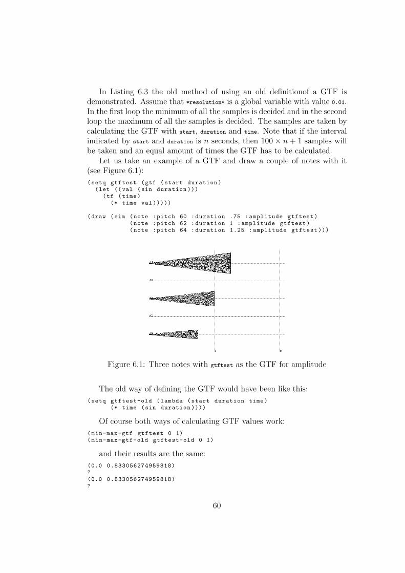
In Listing 6.3 the old method of using an old definitionof a GTF isdemonstrated. Assume that *resolution* is a global variable with value 0.01.In the first loop the minimum of all the samples is decided and in the secondloop the maximum of all the samples is decided. The samples are taken bycalculating the GTF with start, duration and time. Note that if the intervalindicated by start and duration is n seconds, then 100× n + 1 samples willbe taken and an equal amount of times the GTF has to be calculated.

Let us take an example of a GTF and draw a couple of notes with it(see Figure 6.1):

(setq gtftest (gtf (start duration)(let ((val (sin duration )))

(tf (time)(* time val )))))

(draw (sim (note :pitch 60 :duration .75 :amplitude gtftest)(note :pitch 62 :duration 1 :amplitude gtftest)(note :pitch 64 :duration 1.25 :amplitude gtftest )))

Figure 6.1: Three notes with gtftest as the GTF for amplitude

The old way of defining the GTF would have been like this:

(setq gtftest-old (lambda (start duration time)(* time (sin duration ))))

Of course both ways of calculating GTF values work:

(min-max-gtf gtftest 0 1)(min-max-gtf-old gtftest-old 0 1)

and their results are the same:

(0.0 0.833056274959818)?(0.0 0.833056274959818)?

60

It is only the efficiency in which these calculations are carried out thatdiffer. Note that in the one second interval 101 calculations will be carriedout. Note that in the old method the expression with the sine in it has tobe calculated 101 times. On line 2 of Listing 6.4 the GTF is calculated oncewith start and duration and the result is a function of only time, representedby:

(tf (time)(* time 0.8414709848078965))

in which no expression makes use of a sine function, because this wasalready calculated. This function of time is now used 101 to calculate thesample values. As you can imagine the time function is more efficient touse than gtftest-old. You can also imagine that with more complex GTFsand longer time intervals the benefit in efficiency will only increase.

6.4 Midi output

During the design and implementation of NoteFun the desire arose to hearthe musical objects that could be constructed with it. This is why a trans-lation of NoteFun objects to midi sequences was an evident thing to imple-ment. A midi sequence is a serie of midi messages that can be interpretedby a synthesizer. Examples of midi messages are commands that select aprogram number and messages that set a note on and off on certain midichannels. Different notes can sound on different channels, each channelhaving its own program number; multiple instruments can sound on thesame moment. For a full description of the midi protocol we direct you toread The complete MIDI 1.0 Detailed Specification.

Translation of pitch related GTFs

To be able to play objects from NoteFun means to be able to have continuouscontrol of the pitch, volume and other aspects which are involved in a note.In midi the pitch of a note can be controlled by a note number. For instance,midi note number 60 corresponds with the pitch of the middle C: 261.63Hzand midi note 61 corresponds with the succeeding semitone of the middleC, a C-sharp of 277.18Hz. Furthermore pitch can be controlled by meansof pitch bend. Every synthesizer has a certain range in which the pitch canbe deviated from the original frequency of a note. This is done by settingthe range first or using the default pitch bend range. Then a note has to beset on on a certain channel, after which pitch bend command can be sendto deviate from the note’s original pitch. This is the method we used to

61

project GTFs, that are used as a note’s pitch, to actual sound. We will nowshow a little example of a glissando and its corresponding midi sequence.

The example is a very short note with a glissando from note 60 to 61.We have taken a short note to keep the length of the corresponding midisequence relatively short.

The NoteFun code look like this: (note :duration .1 :pitch (glissando 60 61))

and the corresponding midi sequence looks like this:

0.000 begin20.000 midi (176 100 0)

0.000 midi (176 101 0)40.000 midi (176 6 48)

0.000 midi (192 80)60.000 midi (224 0 64)

0.000 midi (176 7 102)80.000 midi (144 60 127)

0.010 midi (224 34 64)100.020 midi (224 68 64)

0.030 midi (224 102 64)120.040 midi (224 8 65)

0.050 midi (224 42 65)140.060 midi (224 76 65)

0.070 midi (224 110 65)160.080 midi (224 17 66)

0.090 midi (224 51 66)180.100 midi (224 85 66)

0.100 midi (128 60 127)200.100 end

A graphical representation of this note can be seen in Figure 6.2.

Figure 6.2: A very short note as a glissando

The leftmost column indicates the time on which the midi message isinterpreted. The rightmost column contains numerical representations ofthe midi message itself. We will not go into detail about all the messagesand parameters but just give a very general description of it. The first

62

three midi messages starting with 176 on line 2 to 4, take care of the pitchbend range being set at 48. This means that a note can maximally bedeviated 48 semitones from the original note’s pitch. On line 5 the programnumber is being set to 80. On our synthesizer this is a square lead sound.On line 6 the pitch bend is being set in the middle, so that initially thenote’s original pitch will sound. This is done because previous notes mighthave left the pitch bend at some undesired value that make our currentnote sound off tune. On line 7 we put the volume at our default value.A previous note might have left the volume at an undesired value, e.g.,total silence, so we have to make sure the value is set to default again.On line 8 the ”note on” message is sent and by default it is note number60, the middle C with a velocity of 127. The velocity is an indication forthe force with which a note is being played, comparable with the forceof pressing a piano key. Then for 10 milliseconds the note sounds at itsoriginal pitch until at time = 0.010 a pitch bend message is sent. The pitchbend message, indicated by number 224 has two parameters. The first onerepresent the least significant bytes (LSB) and the second one representsthe most significant bytes (MSB). Every other 10 millisecond the pitchbend value ascends, until at time = 1.000 the note reaches the pitch thatcorresponds with midi note number 61. Lastly a ”note off” message is sentat time = 1.000 that turns the note off, as you might have guessed.

The 10 millisecond period is an arbitrarily chosen period that is usedto generate a finite amount of midi messages corresponding to a conceptualcontinuous representation of a function. Testing with this period lengthproved that the sounds sounded convincingly as if they were really contin-uous, instead of discrete steps in pitch, volume, etc.

Translation of other aspect related GTFs

The method used for other aspects of a note, like volume, are somewhatless complex, as their control structure permits a more direct mapping withfunctions. Let us demonstrate an example in which the volume of a notegoes from maximum (full loudness) to minimum, (total silence) and alsoinspect the corresponding midi sequence.

The NoteFun representation of this note is: (note :duration .1 :amplitude (ramp 1 0)).The corresponding midi sequence is given here:

0.000 begin20.000 midi (176 100 0)

0.000 midi (176 101 0)40.000 midi (176 6 48)

0.000 midi (192 80)60.000 midi (224 0 64)

63

0.000 midi (176 7 127)80.000 midi (144 60 127)

0.010 midi (176 7 114)100.020 midi (176 7 102)

0.030 midi (176 7 89)120.040 midi (176 7 76)

0.050 midi (176 7 64)140.060 midi (176 7 51)

0.070 midi (176 7 38)160.080 midi (176 7 25)

0.090 midi (176 7 13)180.100 midi (176 7 0)

0.100 midi (128 60 127)200.100 end

A graphical representation of this note can be seen in Figure 6.3.

Figure 6.3: A very short note with a fade out.

The first 8 lines of the midi sequence we have already explained in theprevious example. We have not yet explained that midi messages startingwith 176 are special control messages. The first argument of this message isa control number and the second argument is a control value with can takeon values between 0 and 127. The control number for volume is 7. If wewould send the message (176 7 0) we would set the volume to total silenceand if we would send the message (176 7 127) we would set the volume tothe maximum. In our example we let the volume change linearly fromthe maximum to the minimum. In NoteFun we have chosen to indicatethe volume with values between 0 and 1. What our implementation does istranslate these values to volume control messages with corresponding valuesbetween 0 and 127. As you can see the control value gradually changes 127to 0 throughout the duration of the note, just like we desired.

Having explained these two examples we have pretty much covered thekey method of our translation from NoteFun structures to midi sequences.

64

Chapter 7

Final words

As I already mentioned in the Preface, my internship was a valuable timein which I learned a lot. It was a very good opportunity to combine variousof my passions: computer science, higher order programming and music.During my internship I have broadened my insight in the application andcrossing field of informatics and music, not only by working on this assign-ment, but also by talking with people, watching documentaries, readingbooks and by breathing the atmosphere at the MMM group. I think thateverything there is to say about my experiences during my internship al-ready has been said in previous sections, especially in chapters 5 and 6. Ihope for you reading this report was a pleasure.

65

Bibliography

Matlab, the language of technical computing. The Mathworks, 1996.

The complete MIDI 1.0 Detailed Specification - Incorporating all Recom-mended Practices - document version 96.1. The Midi Manufacturers As-sosication, 1997.

Peter Desain and Henk-Jan Honing. Time functions function best as func-tions of multiple times. Computer Music Journal, 16(2):17–34, 1992.

Charles Dodge and Thomas A. Jerse. Computer Music; synthesis, compo-sition and performance. Schirmer, 1997. ISBN 0028646827.

Henk-Jan Honing. The vibrato problem: comparing two solutions. Com-puter Music Journal, 19(3):32–49, 1995.

Guy L. Steele Jr. Common Lisp : The language. Digital Press, 1990. ISBN1555580416.

Peter Norvig. Paradigms of Artificial Intelligence Programming. MorganKaufmann, 1992. ISBN 1558601910.

Curtis Roads. The Computer Music Tutorial. MIT Press, 1996. ISBN0262680823.

David A. Watt. Programming Language Concepts and Paradigms. PrenticeHall, 1990. ISBN 0137288662.

66