11-1

Note 11 Rotational Motion IISections Covered in the Text: Chapter 13

We continue here with the study of the dynamics ofrotational motion. Towards the end of this note weshall review some of the physics you will encounter inthe experiment “The Compound Pendulum” in thelaboratory. We consider some simple problems ofstatics and continue with rotational energy andangular momentum.

Rotational DynamicsConsider the hypothetical case of a small rocket ofmass m attached to the end of a rigid massless rodpivoted from an immovable point (Figure 11-1). Weconsider the rocket as a single point particle. Therocket is pointing in an arbitrary direction φ withrespect to the rod and the thrust of the rocket engineproduces a force on the end of the rod as shown. Youshould be able to see that the rocket and rod will spinas one system counterclockwise at a steadilyincreasing speed.

Figure 11-1. The hypothetical case of a rocket attached to theend of a rigid massless rod.

The force of the engine

€

r F thrust is resolvable into

transverse and radial components F t and F r. Ft givesthe system a tangential acceleration at, i.e., causes therocket to change speed. The resultant of the tensionforce T and Fr causes the rocket to change direction.Thus we have

€

Ft = mat = mrα , …[11-1]

where α is the angular acceleration of the system(Note 10). Multiplying both sides of eq[11-1] by r weget

€

rFt = mr2α . …[11-2]

The left hand side of eq[11-2] is just the torqueproduced by the force about the pivot. Thus we havefinally

€

τ = mr2α . …[11-3]

We shall see in the next section that we shall find itconvenient to define the quantity mr2 as the moment ofinertia of the mass m about the pivot. In so doing weshall arrive at the rotational analogue of Newton’sSecond Law.

Moment of Inertia andNewton’s Second Law

We now move from a single point particle to a solidrigid body. It is convenient for the moment to think ofthe body as a collection of point particles. Thecollection is constrained by an axis of rotation (Figure11-2). Three arbitrary point particles are shown in thebody along with the force each receives. The wholecollection rotates with the same angular acceleration αabout the rotation axis.

Figure 11-2. Three forces applied to arbitrary positions in arigid body.

The net torque produced by the forces is the sum oftorques

Note 11

11-2

€

τ net = τ ii∑ = miri

2α( )i∑ = miri

2

i∑

α .…[11-4]

where i runs over all the particles in the collection. Wenow define the sum within brackets as the moment ofinertia of the collection. It is conventionally denoted I:

€

I = m1r12 + m2r2

2 + ...= miri2

i∑ . …[11-5]

The units of moment of inertia are kg.m2. A body’smoment of inertia, like torque, depends on the axis ofrotation. Once the axis is specified, so that the ri can bedetermined, then the moment of inertia about thataxis can be calculated from eq[11-5].

Eqs[11-4] and [11-5] allow us to write the angularacceleration as

€

α =τ netI

. …[11-6]

This is just the rotational equivalent of Newton’sSecond Law (a = F/m).

Most bodies of interest are not collections of pointparticles but rather are continuous distributions ofmass. We can depict this by replacing the individual“particles” with cells 1,2,3… each of mass Δm. Thisamounts to converting the moment of inertiasummation to an integration

€

I = ri2Δm = lim

Δm→0ri2Δm∑( )

i∑ = r2dm∫ .

…[11-7]

where r is the distance from the rotation axis. If we letthe rotation axis be the z-axis then we can write themoment of inertia as

€

I = x 2 + y 2( )dm∫ . …[11-8]

The trick in successfully applying eq[11-8] to a specificbody and a specific axis is to replace dm by theappropriate expression in dx and/or dy . Muchpractice in doing this is given in a first year course incalculus. Let us consider an example.

Example Problem 11-1Moment of Inertia of a Rod about a Pivot at one End

Calculate the moment of inertia of a thin, uniform rodof length L and mass M that rotates about a pivot atone end.

Solution:We take the line of the rod as the x-axis and put theend of the rod at x = 0. The rod is thin so we canassume y ≈ 0 for all points on the rod. We imagine therod divided into an infinite number of mass elementsdm each of length dx (Figure 11-3). According to thedefinition eq[11-8]:

Figure 11-3. Finding the moment of inertia about one end ofa long thin rod.

€

I = x 2dm∫ . …[11-9]

Now

€

dm =ML

dx , …[11-10]

and the rod extends from x = 0 to x = L. Thus eq[11-9]becomes

€

Iend =ML

x 2dx =ML

x 2

3

0

L=13ML2

0

L

∫ . …[11-11]

The answer is seen to be simple in form.

Very often if you need an expression for the momentof inertia of a body of simple shape, you need notcalculate the expression from from first principles, butsimply look it up in a table. Figure 11-4 illustrates anumber of bodies of simple shape and their momentsof inertia about major axes. In a typical exam or testquestion you will be given the necessary formula; youwill NOT be required to memorize these formulas.

Note 11

11-3

Figure 11-4. Some examples of the moments of inertia aboutmajor axes of bodies of simple shape. These examples aregiven for purposes of comparison. You will NOT beexpected to memorize these formulas.

The Parallel Axis TheoremThe moment of inertia of a body about an axis ofsymmetry or other axis of convenience is often givenin a table. But sometimes you need to know themoment of inertia of the body about some other,parallel, axis (Figure 11-5). In this case you needn’tcalculate the moment of inertia from first principles.All you need to do is use the so-called Parallel AxisTheorem. The parallel axis theorem states that themoment of inertia I of a body about an axis that isparallel to the axis through the centre of mass adistance d away is

Figure 11-5. Rotation about an off-centre axis.

€

I = Icm + Md2 . …[11-12]

where Icm is the moment of inertia of the body aboutan axis through the centre of mass.

We can easily prove eq[11-12] for a one dimensionalbody pivoted about an axis O (Figure 11-6).

Figure 11-6. Rotation about an off-centre axis.

We define two coordinate systems x and x’, where thepivot is at x = 0 and the centre of mass is at x’ = 0. Thecentre of mass is located a distance d from the pivotpoint. Thus we have x’ = x – d. By definition the

Note 11

11-4

moment of inertia about O is

€

I = x 2dm = x '+d( )2dm = x '2 +2dx '+d2( )dm∫∫∫

€

= x '( )2dm + 2d x 'dm + d2 dm∫∫∫

€

= Icm + 2d x 'dm + Md2∫

€

= Icm + Md2 …[11-13]

because the middle term contains the definition of theposition of the centre of mass in the x’ system which iszero. This result will prove useful in the theory for theexperiment “The Compound Pendulum”.

A Rigid Body in EquilibriumWe saw in Note 04 that a body is in a state oftranslational equilibrium if the sum of the externalforces acting on it is zero, that is, if

F = 0∑ . …[11-14a]

Now that we have studied rotational motion (and inparticular Example Problem 10-5) we can add that abody is in a state of rotational equilibrium if the sumof external torques on it is zero:

τ = 0∑ . …[11-14b]

A body is in a state of both translational and rotation-al equilibrium if both conditions, eqs[11-14] aresatisfied.1

You must remember that eqs[11-14] are vector equa-tions. Thus in 3D space eq[11-14a] yields the threecomponent equations:

Fx∑ = 0 Fy∑ = 0 Fz∑ = 0 .

Concurrent and Non-Concurrent ForcesTwo forces are said to be concurrent if they act alongthe same line. Two or more forces can act on a bodyeither concurrently or non-concurrently. Figure 11-7ashows two concurrent forces acting in opposite 1 It is commonly understood that a body is in a state of equil-ibrium if both conditions, eqs[11-14], are satisfied. If in addition, thebody is at rest, then the body is said to be in the special state ofstatic equilibrium.

directions. The torques these forces produce about Oare equal in magnitude and opposite in direction, andtherefore add to zero. The net torque is zero as is thenet force. This body is in a state of translational androtational equilibrium.

Figure 11-7b shows two non-concurrent forces act-ing on a body. These forces are of unequal magnitudeand act in opposite directions. The magnitude of theresultant torque about O produced by these forces isseen to be

Figure 11-7. Two forces act on a body, concurrent forces (a)and non-concurrent forces (b).

τ∑ = 2rF – 2rF = 0 .

This body is therefore in a state of rotational equilib-rium. However, the net force on the body is not zero:

F∑ = 2F – F = F .

This means that though the body is in a state of rota-tional equilibrium, it is NOT in a state of translationalequilibrium. The body will have a translationalacceleration to the right.

In physics, a whole class of problems can bedescribed as static problems, meaning they involve abody at rest. In such problems the body is describedby the conditions of equilibrium. Using these con-ditions we are able to solve for unknown quantities.

Note 11

11-5

We consider two classic examples, a horizontal beamin equilibrium and the leaning ladder.

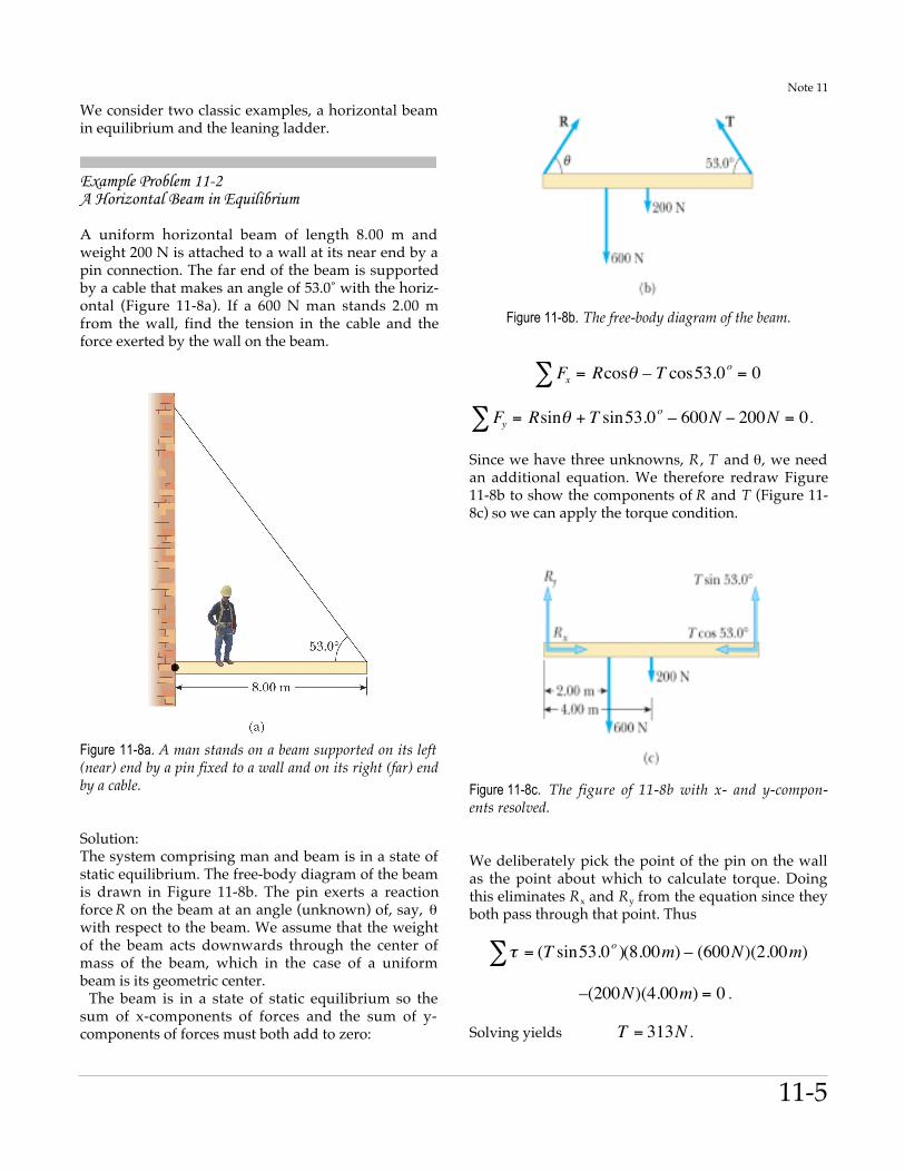
Example Problem 11-2A Horizontal Beam in Equilibrium

A uniform horizontal beam of length 8.00 m andweight 200 N is attached to a wall at its near end by apin connection. The far end of the beam is supportedby a cable that makes an angle of 53.0˚ with the horiz-ontal (Figure 11-8a). If a 600 N man stands 2.00 mfrom the wall, find the tension in the cable and theforce exerted by the wall on the beam.

Figure 11-8a. A man stands on a beam supported on its left(near) end by a pin fixed to a wall and on its right (far) endby a cable.

Solution:The system comprising man and beam is in a state ofstatic equilibrium. The free-body diagram of the beamis drawn in Figure 11-8b. The pin exerts a reactionforce R on the beam at an angle (unknown) of, say, θwith respect to the beam. We assume that the weightof the beam acts downwards through the center ofmass of the beam, which in the case of a uniformbeam is its geometric center.

The beam is in a state of static equilibrium so thesum of x-components of forces and the sum of y-components of forces must both add to zero:

Figure 11-8b. The free-body diagram of the beam.

Fx∑ = Rcosθ – T cos53.0o = 0

Fy∑ = Rsinθ + T sin53.0o – 600N − 200N = 0 .

Since we have three unknowns, R , T and θ, we needan additional equation. We therefore redraw Figure11-8b to show the components of R and T (Figure 11-8c) so we can apply the torque condition.

Figure 11-8c. The figure of 11-8b with x- and y-compon-ents resolved.

We deliberately pick the point of the pin on the wallas the point about which to calculate torque. Doingthis eliminates Rx and Ry from the equation since theyboth pass through that point. Thus

τ = (T sin53.0o )∑ (8.00m) – (600N)(2.00m)

–(200N)(4.00m) = 0 .

Solving yields T = 313N .

Note 11

11-6

Substituting T into the two equations above we get

Rcosθ = 188N

and Rsinθ = 550N .

Dividing the second equation by the first we get

tanθ = 550N188N

= 2.93

and therefore θ = 71.1o

Finally, R = 188Ncosθ

=188Ncos71.1o

= 581N .

The tension in the rope is 313 N. The reaction forceexerted by the wall on the beam is 581 N at an angleof 71.1˚ with respect to the beam.

Example Problem 11-3The Leaning Ladder Problem

A uniform ladder of length l and mass m rests againsta smooth, vertical wall (Figure 11-9a). If the coeffic-ient of static friction between the ladder and ground isµs = 0.40, find the minimum angle θmin at which theladder will not slip.

Figure 11-9a. The leaning ladder problem.

Solution:The ladder is not moving in any way and is thereforein a state of static equilibrium. The free-body diagramof the ladder is drawn in Figure 11-9b. We take x- andy-axes in the horizontal and vertical directions,

respectively. Applying the force condition, eq[11-14a]gives

Fx∑ = f – P = 0 ,

and Fy∑ = n – mg = 0 .

Figure 11-9b. The free-body diagram of the ladder.

Here f is the force of static friction the ground exertson the ladder. R is the vector resultant of f and thenormal force n . P is the normal force the wall exertson the ladder (the wall is smooth so the force of staticfriction between wall and ladder at that point isassumed to be negligible). Thus we have immediatelyn = mg. We apply the torque condition, eq[11-14b],about O because that is the point through which mostof the forces pass. Thus

τ0∑ = Plsinθ – mg l2cosθ = 0 .

This expression applies at just the stage when theladder is about to slip (or rotate about O), that is, at θ= θmin. Thus, rearranging and substituting values weget

tanθmin =mg2P

=n

2 fs.max=

n2(µsn)

=1

2(0.40)

= 1.25 ,

and finally θmin = 51o .

This means that the ladder will not slip so long as theangle of inclination exceeds 51˚. Notice that the

Note 11

11-7

minimum angle is independent of the mass of theladder; it depends only on µs.

Rotational EnergyA rotating body possesses rotational kinetic energy bydefinition because the particles making up the bodyalso rotate. Consider three arbitrary particles in arotating body (Figure 11-10). Assume the body isrotating about a fixed axis (axle).

Figure 11-10. Three arbitrary particles are shown in arotating body.

All particles in the body rotate with the same angularspeed ω. A particle i of mass m i moves in a circle ofradius r i with speed vi = ωri. Thus the total rotationalkinetic energy of the body is the sum of the kineticenergies of the particles:

€

Krot =12m1v1

2 +12m2v2

2 + ...= 12m1r1

2ω 2 +12m2r2

2ω 2 + ...

€

=12

miri2

i∑

ω 2 =

12Iω 2 , …[11-15]

where I is the moment of inertia of the body about theaxle chosen.

In the event that the rotation axis does not passthrough the centre of mass then rotation of the bodymay cause the centre of mass to move up or down. Inthat case, the body’s gravitational potential energy Ug= Mgycm will change. If the system is isolated (i.e., noenergy is lost to dissipative forces and no work isdone on the body from outside) then the body’s totalmechanical energy

€

Kmech = Krot +Ug =12Iω 2 + Mgycm

is conserved. Let us consider an example.

Example Problem 11-4Finding the speed of a Rotating Rod

A rod of length 1.0 m and mass 200.0 g is hinged atone end and connected to a wall (Figure 11-11). It isheld out horizontally, then released. What is the speedof the tip of the rod as it hits the wall?

Figure 11-11. A before- and-after representation of the rod.

Solution:Mechanical energy is conserved so we equate therod’s final mechanical energy (at position 1) to itsinitial mechanical energy (at position 0):

€

12Iω1

2 + Mgycm1 =12Iω0

2 + Mgycm0 .

The initial conditions are ω0 = 0 and ycm0 = 0. Thecentre of mass moves to ycm1 = –L/2 as the rod hits thewall. Using I = (1/3)ML2 for a rod rotating about oneend (Figure 11-4) we have

€

12Iω1

2 + Mgycm1 =16ML2ω1

2 −12MgL = 0

Solving for the rod’s angular velocity we get

Note 11

11-8

€

ω1 =3gL

.

The tip of the rod is moving in a circle of radius r = L .Thus the final speed of the tip is

€

vtip =ω1L = 3gL = 5.42 m.s−1 .

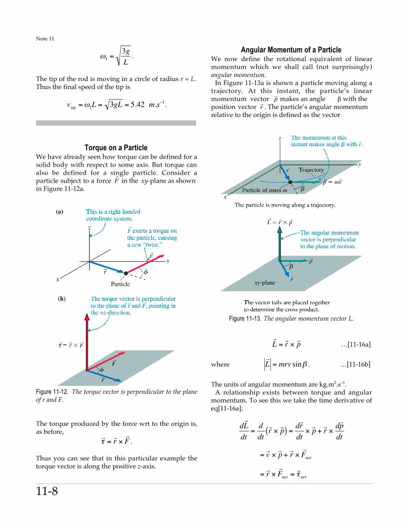
Torque on a ParticleWe have already seen how torque can be defined for asolid body with respect to some axis. But torque canalso be defined for a single particle. Consider aparticle subject to a force

€

r F in the xy-plane as shown

in Figure 11-12a.

Figure 11-12. The torque vector is perpendicular to the planeof r and F.

The torque produced by the force wrt to the origin is,as before,

€

r τ =

r r ×r F .

Thus you can see that in this particular example thetorque vector is along the positive z-axis.

Angular Momentum of a ParticleWe now define the rotational equivalent of linearmomentum which we shall call (not surprisingly)angular momentum.

In Figure 11-13a is shown a particle moving along atrajectory. At this instant, the particle’s linearmomentum vector

€

r p makes an angle β with theposition vector

€

r r . The particle’s angular momentumrelative to the origin is defined as the vector

Figure 11-13. The angular momentum vector L.

€

r L = r r × r p …[11-16a]

where

€

r L = mrv sinβ . …[11-16b]

The units of angular momentum are kg.m2.s–1.A relationship exists between torque and angular

momentum. To see this we take the time derivative ofeq[11-16a]:

€

dr L

dt=

ddt

r r × r p ( ) =dr r dt×

r p + r r × dr p dt

€

=r v × r p + r r ×

r F net

€

=r r ×

r F net =

r τ net

Note 11

11-9

Thus

€

dr L

dt=

r τ net …[11-17]

Eq[11-7] follows because

€

r v and

€

r p are parallel andtherefore their cross product is zero. Eq[11-17] statesin words that a net torque causes a system’s angularmomentum to change. It is the rotational equivalent ofNewton’s Second Law.

Angular Momentum of a Rigid BodyWe can easily extend Eq[11-17] to apply to a rigidbody consisting of a collection of particles. The totalangular momentum of such a system is just the vectorsum:

€

r L =

r L 1 +

r L 2 +

r L 3 + ...=

r L i∑ . …[11-18]

Combining eqs[11-17] and [11-18] we get

€

dr L

dt=

dr L i

dt=

r τ i

i∑

i∑ =

r τ net …[11-19]

The only forces that contribute to the net torque arethe forces exerted on the system by the environment(external forces). The forces producing torquesinternal to the system cancel out (Newton’s ThirdLaw).

Conservation Law of Angular MomentumRecall that for an isolated system the total linearmomentum is conserved. By the same token, for anisolated system (one for which

€

r τ net = 0 ) the angular

momentum is conserved. Or in other words, the finalangular momentum

€

r L f is equal to the initial angular

momentum

€

r L i . Please note that if the angular

momentum is conserved, then both the magnitudeand the direction of the angular momentum vector areunchanged.

Angular Momentum and Angular VelocityAngular momentum and angular velocity are relatedby

€

v L = I r

ω …[11-20]

and as shown in Figure 11-14.

Figure 11-14. The angular momentum vector of a rigid bodyrotating about an axis of symmetry.

Note 11

11-10

AddendumCalculation of the Moment of Inertia of a Rectangular Flat Plate

The pendulum used here is not exactly a rod in thestrictest sense of the word because its width is notzero. A steel ruler is in fact a flat rectangular plate—albeit an elongated one. This means that itsmoment of inertia about its end is given onlyapproximately by eq[3-8]. Let us calculate it prop-erly now to see how good an approximation ofeq[3-8] it is.

Consider a flat plate (ruler) of length l and widthw (Figure 3-4).

xy

dxdy

CMO

l

w

Figure 3-4. An element of area dA in a rectangular plate.

This object is flat, with a thickness that is definitelynegligible in comparison to its other dimensions.The basic definition of the moment of inertia I of aflat object is

€

I = σr2dA = σr2dxdyx∫

y∫∫∫ …[A-1]

where σ is the object’s surface mass density and rlocates an element of area dA relative to the axis ofinterest.

Let us first calculate the moment of inertia of thisobject about an axis perpendicular to the objectand passing through its center—its center of mass(CM). Later we can apply the parallel axis theoremto get the moment of inertia about the point O atits end. Substituting r2 in terms of x and y andinserting the upper and lower limits of x and y intoeq[10] we get the double integral

€

ICM = σ x 2 + y 2( )−l2

l2

∫−w2

w2

∫ dxdy . …[A-2]

Now σ is a constant with the value M/lw. Taking σoutside the integral in eq[A-2] and integrating firstover y we get

€

ICM =Mlw

x 2y +13y 3

−l2

l2

∫−w2

w2

dx ,

€

=Mlw

x 2w +112w3

−l2

l2

∫ dx ,

€

=Mlw

13x 3w + x w

3

12

−l2

l2

.

Substituting the limits and simplifying the finalresult we get

€

ICM =112

M l2 + w2( ) . …[A-3]

According to the parallel axis theorem the moment ofinertia about the endpoint O is given by

€

I0 = ICM + Md2 , …[A-4]

where d is the distance that O is located relative toCM. This distance here is l/2. Thus substituting thisfact and eq[A-3] into eq[A-4] we get

€

I0 =112

M l2 + w2( ) +14Ml2 ,

which, when simplified, is

Note 11

11-11

€

I0 =112

M 4l2 + w2( ) . …[A3-5]

Clearly, if w2 << 4l2, that is, if the width is neglig-

ible in comparison to twice the length, then eq[A3-5] reduces to eq[3-8].

Note 11

11-12

To Be Mastered

• Definitions: angular displacement, radian, average angular velocity, average angular speed, instantaneous angularvelocity, instantaneous angular acceleration, average angular acceleration

• equations of rotational kinematics (to be memorized):

ω f = ωi +αt θ f = θi +ωit +12αt 2 θ f = θi +

12(ω i +ω f )t ω f

2 = ωi2 + 2α(θ f – θi )

• relations between the magnitudes of translational and rotational quantities

x =θr v =ωr a = αr =ω 2r

Typical Quiz/Test/Exam Questions

1. (a) Define torque(b) What are the units of torque?

2. State the following as being a vector or a scalar. Give the units of each.(a) coefficient of friction(b) potential energy(c) linear momentum(d) angular velocity

3. A body is subject to non-concurrent forces. Write down the conditions for the body to be in a state ofmechanical equilibrium. Explain the meaning of each quantity in your expressions.

4. A uniform plank of length 2.00 m and weight 100.0 N is to be balanced on a fulcrum or support point (see thefigure). A 500.0 N weight is suspended from the right end of the plank and a 200.0 N weight suspended fromthe left end. Answer the following questions.

left right

fulcrum

(a) Describe the state of the plank when it is balanced.(b) What are the conditions for this state?(c) How far from the left end of the plank must the fulcrum be placed?(d) What is the reaction force exerted by the fulcrum on the plank?