Barcelona GSE Working Paper Series

Working Paper nº 1063

Not so Disruptive after All: How Workplace Digitalization Affects Political Preferences

Aina Gallego Thomas Kurer Nikolas Schöll

November 2018

Not so Disruptive after All: How Workplace Digitalization

Affects Political Preferences∗

Aina Gallego †

Thomas Kurer ‡

Nikolas Schöll §

November 23, 2018

Abstract

New digital technologies are transforming workplaces, with unequal economic con-

sequences depending on workers’ skill set. Does digitalization also cause divergence in

political preferences? Using an innovative empirical approach combining individual-

level panel data from the United Kingdom with a time-varying industry-level measure

of digitalization, we first show that digitalization was economically beneficial for a

majority of the labor force between 1997-2015. High-skilled workers did particularly

well, they are the winners of digitalization. We then demonstrate that positive eco-

nomic trajectories are mirrored in political preferences: Among high-skilled workers,

exposure to digitalization increased voter turnout, support for the Conservatives, and

support for the incumbent. An instrumental variable analysis, placebo tests and multi-

ple robustness checks support our causal interpretation. The findings complement the

dominant narrative of the "revenge of the left-behind": While digitalization undoubt-

edly eliminates some jobs and does produce losers, there is a large and often neglected

group of winners of digitalization who positively react to economic modernization by

supporting the status quo.∗Acknowledgements: We thank Ruben Enikolopov, Albrecht Glitz, Maria Petrova, Henning Finser-

aas, Torben Iversen, Carles Boix, Markus Prior, Marius Busemeyer, Julian Garritzman, Susanne Garritz-man, Ben Ansell, Jane Gingrich, Michael Donnelly, Paul Marx, Bruno Palier and seminar participantsat Universitat Pompeu Fabra, Universitat de Barcelona, Duisburg University, Nottingham University,University of Konstanz, University of Geneva, University of Amsterdam, Sciences Po, and conference at-tendants at APSA and ECPR for helpful comments and suggestions. The research leading to these resultshas received funding from the Spanish Ministry of Economy and Competitiveness (MINECO) under theCSO2016-79569-P and from the BBVA Foundation through the project "Digital technology, ideologicalpolarization and intolerance." The three authors have contributed equally to this manuscript.†Institut Barcelona d’Estudis Internacionals and IPEG. E-mail: agallego@ibei.org‡Harvard University. E-mail: tkurer@wcfia.harvard.edu§Universitat Pompeu Fabra, IPEG and Barcelona GSE. E-mail: nikolas.schoell@upf.edu

1 Introduction

Technological innovations have a long history of producing economic change and political

upheaval (Caprettini and Voth, 2017; Mokyr, Vickers and Ziebarth, 2015; Boix, 2015).

A recurring preoccupation is that new machines replace human workers, create impov-

erishment, and produce political instability. This century-old concern is currently seeing

a revival. Anxiety about automation is again widespread among the public. In 2017,

according to the Eurobarometer, 72% of respondents agreed with the statement that dig-

ital technologies such as robots and artificial intelligence destroy jobs. Media pundits

increasingly voice concerns that job displacement induced by new digital technologies has

contributed to the recent political disruptions in many countries. An opinion piece in the

New York Times, for example, draws on work in labor economics to argue that "robots [...]

helped elect Trump" (Edsall, 2018). A central worry in the "fear of the robots" narrative

is that workers displaced by digital technologies are turning against the political status

quo.

Rigorous scholarly evidence on the political consequences of digitalization is still too

scarce to draw firm conclusions. Recent work suggests that workers susceptible to automa-

tion demand more redistribution (Thewissen and Rueda, 2017), become more likely to

vote for Trump (Frey, Berger and Chen, 2018) or increasingly support radical right parties

(Dal Bó et al., 2018). Our contribution builds on this emerging literature but attempts to

improve the existing body of work in three respects. The first concern is operationalization:

Existing studies rely on indirect indicators of digitalization based on the prevalence of rou-

tine tasks in an occupation. This is in line with seminal contributions in labor economics

but time-invariant indicators do not capture changes in the penetration of technology at

the workplace and do not allow disentangling the effect of risk of substitution by digital

technologies from a myriad other occupational characteristics. A second limitation relates

to identification and selection bias of workers into workplaces. The kind of worker who

prefers more redistribution or is sympathetic to candidates such as Donald Trump might

self-select into routine occupations or into manufacturing areas with high exposure to risk.

In that case, the observed correlations between routine work and political attitudes would

not necessarily be related to the introduction of digital technologies.

Our more substantive critique is that the focus in both public discourse and academic

1

work on the losers of digitalization is overly narrow.1 We do not dispute that a part of the

population has difficulties to adapt to changing skill requirements in an increasingly digi-

talized work environment, or that digitalization eliminates jobs and indeed produces losers.

But an exclusive focus on citizens experiencing disadvantages might paint an incomplete

picture of the political repercussions of economic modernization (see also Iversen and Sos-

kice, 2019). It is at odds with standard economic theory, which claims that technological

innovations increase productivity and wages – and thereby produce at least as many win-

ners as losers. It is also at odds with historical experience, which has failed to produce the

mass technological unemployment dreaded by Marx, Keynes, Leontief and many others.

A more comprehensive understanding of the political consequences of digitalization should

also study workers who benefit from it.

This paper improves on all three limitations in existing work. To address concerns about

operationalization, we use a more direct measure of digitalization: time-varying indicators

of ICT capital stocks at the industry-level (covering 1997-2015) taken from the EU KLEMS

database (see also Michaels, Natraj and Van Reenen, 2014). For identification, we rely on

rich individual-level panel data from the British Household Panel Study (BHPS) and the

Understanding Society survey (UKHLS) and fixed effects models, which allow us to control

for time-invariant individual and industry-level characteristics. An instrumental variable

approach, a placebo analysis using non-ICT capital instead of ICT capital and multiple

robustness checks add confidence to a causal interpretation of our findings. Finally, our

approach is well-suited to study the large group of beneficiaries of technological change.

Using a representative sample of the labor force, we show that labor market outcomes and

political behavior of workers change when their industries become more intense in ICT

capital and, crucially, that these effects vary depending on the workers’ education level.

Our results suggest that digitalization at the workplace is economically beneficial for a

majority of the workforce. ICT capital in an industry increases the salaries of all but the

least educated workers and has limited adverse employment effects. Turning to political

outcomes, our findings show that these distributive implications are reflected in individual

political reactions to technological change. Faster than average digitalization is associated

with increased (a) voter turnout, (b) support for the Conservative party, and (c) support1This is at least partly a consequence of an influential study estimating that digitalization puts almost

every second job at high risk of disappearing in the near future (Frey and Osborne, 2017). Although thisfigure has been questioned by later studies (see, e.g., Arntz, Gregory and Zierahn, 2016), the emphasis ondisplaced workers endures.

2

for the incumbent, but only among winners of digitalization, that is the highly educated.2

Digitalization is unrelated or negatively related to the turnout rates of less educated workers

and has no discernible effect on their support for parties.

To the best of our knowledge, this is the first paper to produce well identified individual-

level effects of workplace digitalization on political outcomes using panel data.3 We shed

new light on the political consequences of digitalization by highlighting its multi-faceted

effects. The finding that digitalization is economically beneficial for a majority of workers

and that these workers increasingly support center-right mainstream and incumbent parties

is in line with standard economic theory. This finding does not preclude that some sectors

suffer in absolute or relative terms, and we indeed find evidence of economic polarization.

Still, our paper brings attention to economic winners, a neglected population in the large

literature on the political implications of structural change, and adds nuance to the gloomy

picture in the "fear of robots" narrative. Technological change does not only shape politics

by creating a reservoir of dissatisfied losers who find the political remedies offered by

populist or anti-establishment parties appealing, but it can also increase support for the

establishment among the large group of beneficiaries.

2 The political implications of technological change

A large theoretical and empirical literature in labor economics studies how advances in

technology affect economic outcomes such as salaries, employment, and income inequality

(e.g. Berman, Bound and Machin, 1998; Autor, Levy and Murnane, 2003; Autor, Katz and

Kearney, 2006; Goldin and Katz, 2009; Goos, Manning and Salomons, 2009; Acemoglu

and Restrepo, 2017). At a very general level, the effects of technological change on wages

and employment depend on the net outcome of two countervailing forces (Acemoglu and

Restrepo, 2018). The painful aspect of technological change is that it creates a displacement

effect as machines start to perform tasks previously done by humans. The benign aspect is

a productivity effect. New technologies complement workers, for example when they allow

for quick communication with colleagues. They free up time spent doing dull tasks, which2As we discuss later, we find that education strongly conditions whether workers benefit or not from

workplace digitalization. We also replicate the analysis distinguishing between workers in occupations withhigh or low routine-task intensity, but we do not find similarly strong moderation by routineness.

3Most studies about the consequences of technological change in economics analyze aggregate leveloutcomes rather than the effects on the individual trajectories of workers (for an exception see Dauthet al., 2017). We also contribute to this literature by examining how workers’ wages and probability ofunemployment change when their industries digitalize.

3

can be spent more productively. They thus reduce the cost of tasks, generating economic

growth and an increase in the demand for labor. Finally, new technologies create entirely

new jobs, such as when computers generated demand for software engineers.

The net effect of these two forces on wages and employment is a priori uncertain. In the

last two centuries, however, the productivity effect of technological has clearly dominated

(Mokyr, Vickers and Ziebarth, 2015). Technological change, along with well-designed,

complementary institutions, is the most important cause of the unrivaled growth in output

and living standards since the Industrial Revolution. While perhaps less impressive than

in the 1960s, the overall positive economic effect of technological innovation still holds

today (Mokyr, 2018). The long-term macro picture might offer little consolation for work-

ers displaced by technology, but it suggests that mass inmiseration due to technological

change is rare and that most individuals have historically benefited from technology-driven

productivity gains.

Average positive effects on wages are compatible with significant heterogeneity. The

specific distributive effects depend crucially on the complementarities or substitution effects

between new technologies and workers’ skills. The last wave of technological innovation,

which is characterized by the extension of information and communication technologies

(we use the term digitalization to analytically distinguish from the more generic term of

technological change), has mostly benefited highly educated workers while the detrimental

effects are concentrated on less skilled workers and those in routine occupations (Autor,

Levy and Murnane, 2003; Michaels, Natraj and Van Reenen, 2014; Goos, Manning and

Salomons, 2009). We expect highly educated workers to benefit most from digitalization,

but existing studies are somewhat ambiguous on the crucial question whether we should

expect workers with low or mid levels of skills to become worse off when their workplace

digitalizes. Most studies analyze the aggregate economic impact of technological change

across countries, industries or regions rather than changes within individuals. For the

purposes of our study it is important to note that the well-documented reduction in jobs

in mid-paying occupations does not necessarily imply that at the micro level workers with

intermediate levels of skills suffer most. This is one of the empirical questions we set to

explore.4

4The observed aggregate reductions in mid-paying jobs can be driven by retirement (a non-traumaticway to exit the labor market) without replacement being concentrated in these jobs, and by exits to otherjobs which are often higher paying (Dauth et al., 2017; Cortes, 2016). If both processes are at work,we should not necessarily observe that digitalization decreases the salaries or increases the probability to

4

Despite the evident distributive consequences of digitalization, the political implications

of this economic transformation have received little academic attention (notable exceptions

are the above-mentioned papers by Thewissen and Rueda (2017), Frey, Berger and Chen

(2018), and Dal Bó et al. (2018)). This stands in sharp contrast to the extensive litera-

ture on the implications of globalization and international trade (Margalit, 2011; Jensen,

Quinn and Weymouth, 2017; Autor, Hanson and Majlesi, 2016; Colantone and Stanig,

2018a,b). This neglect is noteworthy since the empirical evidence suggests that techno-

logical change is the most important driver behind the transformation of the employment

structure and outperforms international trade and migration as an explanation of the rise

in inequality and job polarization (Jaumotte, Lall and Papageorgiou, 2013; Goos, Manning

and Salomons, 2014).

To generate our hypotheses on political outcomes, we build on three core theories of

political behavior – resource model of participation, spatial or ideological voting, and eco-

nomic voting– which point to three distinct but in principle equally likely ways in which

digitalization can affect political behavior. In all cases, we expect the effects of digital-

ization at the workplace to be heterogeneous depending on whether workers are likely

to benefit from it or not. Previous work has proposed different reasons why digitaliza-

tion may affect the political behavior of the disadvantaged (or "left behind"), but we are

just as interested in the inversion of these theories’ arguments, and hence discuss explicit

expectations with respect to both less and highly educated workers.

We concentrate on education rather than on task content, i.e. the distinction between

routine vs non-routine occupations dominant in economics (Autor, Levy and Murnane,

2003; Goos, Manning and Salomons, 2009), for theoretical and empirical reasons. Educa-

tion is a generally stable individual characteristic, as relatively few people acquire higher

educational credentials after finishing schooling in young adulthood. Intra-individual sta-

bility makes education more suited for our longitudinal analysis than routine task intensity

(RTI), which is measured on the level of occupations and changes as workers switch be-

tween different jobs. RTI is hence a fluid and potentially endogenous characteristic giving

rise to varied trajectories.

More importantly, education should be correlated with individuals’ unobserved cogni-

tive skills and ability to learn and hence with their potential to adapt to and reap the

become unemployed of individuals.

5

benefits of the introduction of new digital technologies in the workplace. By contrast, it is

unclear if the current RTI of a worker’s job is informative about his or her ability to adapt

to digitalization. For instance, a highly educated routine worker (e.g. an accountant) may

have the cognitive resources to adapt to the introduction of software that performs rou-

tine accounting tasks, and become more productive at the same or another job, a process

known as upskilling (Hershbein and Kahn, 2018). In our empirical setting, which inter-

acts an industry-level variable of economic change with an individual trait capturing the

capability to deal with this development, education is more informative about the ability

to learn, retrain, and ultimately benefit from digitalization than routine task content of

the current job. We support this claim with empirical evidence in section S3 where we

show that education is a stronger moderator than RTI in predicting whether workers are

positively or negatively affected by digitalization in their industries.

2.1 Digitalization and voter turnout

Our first expectation is that exposure to digitalization may affect participation in elections

and that this effect is heterogeneous depending on whether workers benefit economically or

are harmed by the introduction of new technologies in their workplaces. This can happen

mainly through three mechanisms. The vast literature on the resource model of political

participation (e.g. Verba, Schlozman and Brady, 1995) generates the expectation that

economic hardship and a reduction of resources leads to lower turnout. If digitalization

reduces wages among workers with less education who can be substituted by machines

but increases wages among highly educated workers with skills that are complements to

machines, we expect the political participation of these two groups to diverge when their

workplaces digitalize.

A second mechanism with the potential to affect voter turnout is job insecurity or

even job loss. In particular unemployment might lead to "political withdrawal" as citizens

concentrate in solving more pressing problems than participation in elections (Rosenstone,

1982). Again, digitalization has contrasting effects on job prospects, as less educated

workers become less secure in their jobs if the tasks they perform can be done by machines

while the demand for highly educated workers increases if they become more productive.

Although results about the relationship between unemployment and job security on voter

turnout are mixed (Smets and Van Ham, 2013), recent evidence suggests that labor market

6

vulnerability tends to go hand in hand with less political participation (Rovny and Rovny,

2017), and this demobilizing effect is especially pronounced in contexts where unemploy-

ment is not excessively high (Aytaç, Rau and Stokes, 2018), which is the case in the UK

in the period we study. Importantly, research using similar longitudinal panel data shows

that unemployment and insecurity can reduce political engagement (Emmenegger, Marx

and Schraff, 2017).

A third mechanism through which workplace digitalization can affect political partic-

ipation is psychological. The realization that tasks previously performed by humans can

be carried out by machines might undermine feelings of self-efficacy and self-esteem, which

are important precursors of political engagement (Marx and Nguyen, 2016). Conversely,

workers with complementary skills may become more central economically and become

politically empowered as a result.

In sum, because of its material and psychological effects, we expect digitalization to

increase political participation among highly educated workers and depress participation

among the less educated, resulting in an increase in inequalities in voter participation.

2.2 Digitalization and party support

Beyond participation in elections, we also expect digitalization to shape preferences for

political parties. Two core models in the study of political behavior, spatial or ideological

voting models and economic voting models, point to two different predictions about the

political consequences of digitalization for workers.

The first relevant stream of research is based on spatial models of voting, which depict

political competition as a conflict about redistributive issues, and individual material cir-

cumstances as the main driver of individual policy preferences (e.g. Margalit, 2013; Rueda,

2005) and ultimately of party support (e.g. Iversen and Soskice, 2006). While theoretical

models diverge in their attention to economic disadvantage (and hence demand for redis-

tribution) or risk (and hence demand for insurance) (Rehm, Hacker and Schlesinger, 2012),

in our case economic disadvantage and risks are bundled: Digitalization can depress wages

and increase risk of displacement for workers who can be substituted by machines, who

typically have low or middle levels of skills. It has the opposite effect on both dimensions

for workers with complementary skills to machines, who are typically highly educated.

Workers affected by digitalization may change their preferences about parties through

7

two channels. The first is changes in their material situation. Increases in income and

job opportunities (or even in expectations) among workers with skills that are complemen-

tary to computers will reduce support for redistribution and increase support for parties

that defend right-wing economic policies. Conversely, less educated workers at risk of

substitution should become more supportive of parties that defend redistribution. These

expectations are consistent with the findings reported in Thewissen and Rueda (2017), who

show in cross-sectional analyses that workers who are likely to be negatively affected by

digitalization demand more redistribution, even after introducing a wide range of controls.

An additional, more speculative, channel through which digitalization can affect sup-

port for parties is by altering attitudes towards the market and regulation. New tech-

nologies facilitate the creation of new markets where workers can directly offer goods and

services. This direct exposure to markets shapes a more positive attitude if the worker

sees herself as a beneficiary of the transformation. In addition, experience with technolog-

ical disruption can make workers skeptical of the ability of government to regulate rapidly

changing sectors, especially for those who expect their career perspectives to improve due

to digitalization and hence have little motivation to demand regulation. Consistent with

this intuition, a recent study of wealthy Americans’ political preferences (Broockman, Fer-

enstein and Malhotra, 2017) found that Silicon Valley’s tech entrepreneurs, a clear group of

winners of digitalization, indeed oppose government regulation and display more market-

friendly attitudes than other Democrats.5

The basic characterization of party competition described in these models applies to

the UK. The main parties have clearly distinct positions on economic issues such as redis-

tribution and social insurance. While the importance of class voting and the alignment of

parties with income groups has declined since the 1970s (Evans and Tilley, 2017), the Con-

servative Party still defends more right-wing economic positions than the Labour Party,

with the Liberal Democratic Party taking intermediary positions. In our setting, we ex-

pect digitalization to increase support for the Conservative Party among highly educated

workers who become better off due to digitalization. Conversely, exposure to digitalization

should increase support for the Labour Party among less educated workers.

A second stream of research suggests that changes in the economic standing of workers5One might ask why people who choose to work in the highly paid tech industry support the Democrats

in the first place. However, party choice is the result of multiple considerations including moral issues,immigration and cosmopolitanism that may motivate tech elites to support a progressive rather than aconservative party.

8

will affect support for the incumbent (Lewis-Beck and Stegmaier, 2000). In retrospective

voting models (Fiorina, 1978), individual’s economic situation influences their support for

the incumbent through a simple punishment-reward mechanism. In the case of digitaliza-

tion, this logic leads us to expect that highly educated workers who are positively affected

by digitalization should become more likely to support the political status quo and hence

the incumbent party. Conversely, less educated workers could become less supportive of

the incumbent.

Some previous research is consistent with digitalization leading to an increase or de-

crease in support for the incumbent depending on how it affects different groups. Frey,

Berger and Chen (2018) study vote for Donald Trump and argue that voters who most

strongly feel the adverse consequences of automation might opt for radical political change,

but their findings can also be interpreted through the prism of classical economic voting.

Research about the political consequences of other structural transformations such as off-

shoring and trade with China finds that voters in negatively affected areas withdraw sup-

port for the incumbent party (Margalit, 2011; Jensen, Quinn and Weymouth, 2017; Autor,

Hanson and Majlesi, 2016). Again, there is evidence from the UK confirming the relevance

of economic voting in this context (Tilley, Neundorf and Hobolt, 2018) as well as, more

generally, the relevance of valence or performance considerations in elections (Clarke et al.,

2004).

These two key expectations on the effects of digitalization for party support are drawn

from well-established models in political behavior research. Both possibilities are a priori

equally plausible and there is no theoretical reason to expect that one should apply but

not the other.6 The period we study covers governments by left- and right-wing political

parties. Note that until 2010, when the Labour Party was in power, the prediction of spatial

voting models is that highly educated workers should become more likely to support the

Conservative Party due to economic self-interest but more likely to support the incumbent

Labour Party due to egotropic economic voting. If both processes occur at the same

time in the pre-2010 period, they would produce effects in opposite directions, potentially

canceling each other out. By contrast, under Conservative government from 2010 onwards,6Note that the processes discussed are based on very general principles and can apply even in the

absence of public debate about the issue of digitalization and technological change and even if workersdo not actively reflect about this topic. The theoretical expectations could vary substantially if partiespoliticized the issue of digitalization. However, the party manifestos in the UK in the period covered bythis study suggest that this topic was hardly mentioned.

9

the two processes produce reinforcing effects. An important implication is that the precise

political consequences of digitalization depend on the specific political situation.

3 Data and descriptive overview

Our empirical analyses focus on the case of the UK, an established democracy at the frontier

of technological innovation for which rich longitudinal micro-level data are available.

3.1 Industry level measure of digitalization

To measure digitalization, we follow Michaels, Natraj and Van Reenen (2014), who use

yearly changes in ICT capital stocks within industries.7 We use the September 2017 release

of the EU KLEMS dataset (Jaeger, 2017), which contains yearly measures of output, input

and productivity for 40 industries in a wide range of countries, including the UK, and

covers the period 1997 to 2017. The data is compiled using information from the national

statistical offices and then harmonized to ensure comparability. Most importantly for

our purposes, the database provides a breakdown of capital into ICT and non-ICT assets

(O’Mahony and Timmer, 2009). This allows for the creation of time-varying, industry-

specific indicators of digitalization based on ICT stocks.

Our measure of digitalization is constructed as follows:

Dj,t “(ICT capital stock in thousand GBPj,t)

(Employeesj,t)

Where ICT capital stockj,t is the sum of the fixed capital stocks in computing equipment,

communications equipment, computer software and databases in industry j in year t, at

constant 2010 prices.8

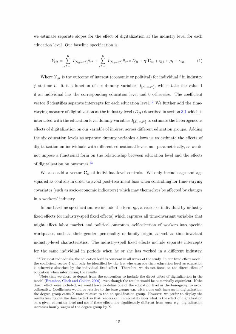
Figure 1 plots the evolution of our indicator of digitalization over time for the industries

provided by EU KLEMS.9 Some industries are disaggregated only at the 1-digit level (e.g.7Our approach is also similar to Graetz and Michaels (2015) and Acemoglu and Restrepo (2017) who

focus on the effects of the introduction of a particular technology, robots, across industries.8Note that productivity-enhancing and potentially labor-saving investments can in principle affect our

measure in two ways. First, they increase the numerator (the ICT capital stock) and second, they canreduce the denominator if labor-saving technologies are implemented and reduce the number of employeesin the industry. This is a manifestation of the two-fold consequences of digitalization: It can be beneficialto the remaining worker by increasing her productivity or threatening to the worker as it reduces labordemand. Our measure hence captures ICT intensity relative to labor in an industry, rather than ICTintensity in an absolute sense.

9EU KLEMS data is disaggregated by 40 industries based on the industry standard classification systemused in the European Union (NACE rev1). For 3 industries, ICT data is missing or has only zero values

10

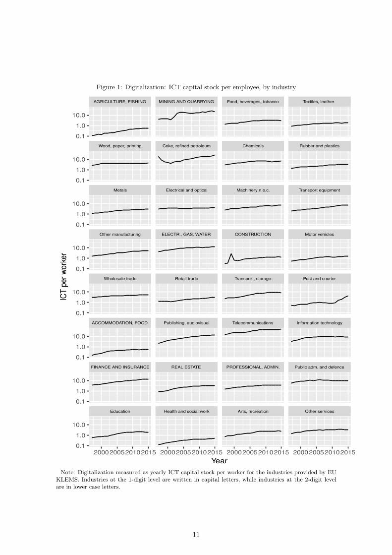
Figure 1: Digitalization: ICT capital stock per employee, by industry

Education Health and social work Arts, recreation Other services

FINANCE AND INSURANCE REAL ESTATE PROFESSIONAL, ADMIN. Public adm. and defence

ACCOMMODATION, FOOD Publishing, audiovisual Telecommunications Information technology

Wholesale trade Retail trade Transport, storage Post and courier

Other manufacturing ELECTR., GAS, WATER CONSTRUCTION Motor vehicles

Metals Electrical and optical Machinery n.e.c. Transport equipment

Wood, paper, printing Coke, refined petroleum Chemicals Rubber and plastics

AGRICULTURE, FISHING MINING AND QUARRYING Food, beverages, tobacco Textiles, leather

2000200520102015 2000200520102015 2000200520102015 2000200520102015

0.1

1.0

10.0

0.1

1.0

10.0

0.1

1.0

10.0

0.1

1.0

10.0

0.1

1.0

10.0

0.1

1.0

10.0

0.1

1.0

10.0

0.1

1.0

10.0

Year

ICT

per

work

er

Note: Digitalization measured as yearly ICT capital stock per worker for the industries provided by EUKLEMS. Industries at the 1-digit level are written in capital letters, while industries at the 2-digit levelare in lower case letters.

11

Agriculture, forestry and fishing), while for other industries EU KLEMS also breaks down

the data at the more fine-grained 2-digit level (e.g. manufacturing is disaggregated into 11

categories such as "food products, beverages and tobacco").

As expected, we see a general increase in the importance of digital technologies over

time. The levels of ICT intensity also vary across industries in a sensible way (e.g. they

are highest for telecommunications, or finance and insurance, as we would expect), adding

to our confidence that the measure is valid. Note that the over time trend shown in the

graph most likely understates the true degree of digitalization as ICT prices fell drastically

over time. However, this does not invalidate our analysis since we will use year fixed effects

and therefore focus on within year variation across industries in the adoption of ICT.

3.2 Individual-level survey data

We combine this measure of digitalization at the industry level with longitudinal data from

the British Household Panel Study (BHPS) and the Understanding Society (UKHLS) sur-

vey. The BHPS is a longitudinal study that has interviewed about 10,000 individuals

nested in 5,000 households drawn from a stratified random sample of the British popula-

tion yearly from 1991 to 2008. In 2009 the BHPS was transformed into the Understanding

Society (UKHLS) survey, with considerably expanded sample size (for a thorough descrip-

tion about survey design see Buck and McFall, 2011). Every year participants are asked

detailed questions about their economic situation, current and past employment, as well

as a few political questions.

We assign every worker the value of our measure of digitalization (ICT per worker) in his

or her current industry. Because the 2017 EU KLEMS release only covers the period since

1997, we exclude respondents surveyed between 1991 and 1996 from our study. We also

drop from our sample respondents aged 65 and older (who should be less affected by changes

in the labor market) and respondents less than 18 year old. Our final BHPS/UKHLS

sample contains 392’967 observations, of which 71.3% can be linked to one of 32 industries

(NACE rev. 2). We exclude extraterritorial organizations and households as employers

as there is no information on ICT capital stocks. Our final sample contains 276’855 for

60’029 individuals.10

which reduces our sample to 37. NACE codes are consistent with UK SIC codes provided in the BHPS,which allows for a comprehensive merge of the two datasets. The scale of the y axis is logged to facilitatevisualization, but the analyses use the original variable, operationalized as discussed above.

10The analyses do not include people not assigned to an industry, including students or the currently

12

The dependent variables in our analyses are a set of indicators of economic situation

and political attitudes asked consistently over time by BHPS/UKHLS.

Wages: We compute hourly net wages in constant 2010 prices using the variable usual

net pay per month, which is derived by BHPS/UKHLS staff using answers to detailed

income questions and imputed if this information is missing. This is normalized by hours

worked. Observations with less than half time employment (20 hours per week) are ex-

cluded from this analysis since there is considerable measurement error which leads to noise

in our calculation if the denominator (hours worked) is small.

Unemployment: The employment status refers to the week when the respondent was

interviewed. The surveys do not ask about unemployment spells between surveys, so we can

only look at the moment of the interview, which is a lower bound for unemployment. Since

we are interested in the effect of digitalization on the probability to become unemployed,

we focus our analysis on the effect of current digitalization of a worker’s industry on her

probability of being unemployed at the time of the next interview.

Voter turnout: Our measure of voter turnout is self-reported participation in the last

general election, which is asked in all waves until 2008 and then in 2010 and 2015.

Support for the Conservative Party and the Labour Party: We construct

this variable using a series of questions asked every year on whether respondents consider

themselves supporters of any particular party or (if they are not) if they feel closer to one

political party than to the others. In the Supporting Information (SI) we also present the

results about support for the Liberal Democratic Party and UKIP.

Support for the incumbent: We code respondents as supporters of the incumbent

party if they supported the Labour Party before the government change in 2010 and the

Conservative Party after it changed.11

In order to examine if the effects of digitalization on the economic and political out-

comes of workers vary depending on their education level, we use information about educa-

tional attainment. It is coded in six categories: university degree (26.6% of the sample in

2015); other higher degree (such as teaching or nursing, 12.4%), A-Level and other higher

secondary qualifications (21%); General Certificate of Secondary Education, O-level and

unemployed if no industry is reported, people who never enter the labor force, and people who have exitedthe labor force.

11Including LibDem as part of the government between 2010 and 2015 does not change the results. TheBHPS/UKHLS asks other questions about political attitudes (such as attitudes towards the role of thegovernment in the economy or nationalism), but only infrequently and mostly in the BHPS period before2008. We concentrate on the variables for which we can obtain a longer time series.

13

other lower secondary qualifications (19%); other qualifications (9.2%); and no formal

qualifications (11.7%).

Table 1 presents the summary statistics of the main variables used in the analyses. The

SI contains a detailed description of the evolution of all dependent variables over time for

each educational group.

Table 1: Summary Statistics

Count Mean SD Min Max

ICT capital stock per worker 276855 2.14 2.46 0.05 25.30

ICT capital stock USA per worker 270019 28.73 83.89 0.18 1041.22

Non-ICT capital stock per worker 276855 132.96 391.58 6.46 4955.94

Hourly wage 223760 9.41 23.94 0.00 5785.66

Probability to become unemployed 213823 0.02 0.15 0 1

Voted in last general elections 108880 0.70 0.46 0 1

Supports the Conservative Party 232121 0.22 0.41 0 1

Supports the Labour Party 232121 0.32 0.47 0 1

Age 276855 40.43 12.02 18 64

Female 276855 0.50 0.50 0 1

Year 276855 2008.54 5.08 1997 2015

Routine Task Intensity 264331 -0.26 0.78 -1.87 2.10

Industry in EUKELMS categories 276855 1 38

Government region ID 275923 1 13

Observations 276855

Note: ICT defined as "real fixed ICT capital stock (in 1000 GBP in constant 2010 prices) normalized bynumber of employees".

4 Estimation and identification

4.1 Fixed-effects model

We use individual industry-spell fixed-effects models to estimate the effects of digitaliza-

tion in a worker’s industry on labor market and political outcomes. As discussed above,

we expect the effects of digitalization on labor market and political outcomes to be het-

erogeneous across workers depending on their education level. To test this expectation,

14

we estimate separate slopes for the effect of digitalization at the industry level for each

education level. Our baseline specification is:

Yijt “

6ÿ

s˚“1

IrSit“s˚sδs˚ `

6ÿ

s˚“1

IrSit“s˚sθs˚ˆDjt ` γ 1Cit ` ηij ` µt ` εijt (1)

Where Yijt is the outcome of interest (economic or political) for individual i in industry

j at time t. It is a function of six dummy variables IrSit“s˚s, which take the value 1

if an individual has the corresponding education level and 0 otherwise. The coefficient

vector δ identifies separate intercepts for each education level.12 We further add the time-

varying measure of digitalization at the industry level (Djt) described in section 3.1 which is

interacted with the education level dummy variables IrSit“s˚s to estimate the heterogeneous

effects of digitalization on our variable of interest across different education groups. Adding

the six education levels as separate dummy variables allows us to estimate the effects of

digitalization on individuals with different educational levels non-parametrically, as we do

not impose a functional form on the relationship between education level and the effects

of digitalization on outcomes.13

We also add a vector Cit of individual-level controls. We only include age and age

squared as controls in order to avoid post-treatment bias when controlling for time-varying

covariates (such as socio-economic indicators) which may themselves be affected by changes

in a workers’ industry.

In our baseline specification, we include the term ηij , a vector of individual by industry

fixed effects (or industry-spell fixed effects) which captures all time-invariant variables that

might affect labor market and political outcomes, self-selection of workers into specific

workplaces, such as their gender, personality or family origin, as well as time-invariant

industry-level characteristics. The industry-spell fixed effects include separate intercepts

for the same individual in periods when he or she has worked in a different industry.12For most individuals, the education level is constant in all waves of the study. In our fixed effect model,

the coefficient vector δ will only be identified by the few who upgrade their education level as educationis otherwise absorbed by the individual fixed effect. Therefore, we do not focus on the direct effect ofeducation when interpreting the results.

13Note that we chose to depart from the convention to include the direct effect of digitalization in themodel (Brambor, Clark and Golder, 2006), even though the results would be numerically equivalent. If thedirect effect were included, we would have to define one of the education level as the base-group to avoidcolinearity. Coefficients would be relative to the base group: e.g. with a one unit increase in digitalization,the degree group earns X more relative to the no qualification group. However, we prefer to display theresults leaving out the direct effect so that readers can immediately infer what is the effect of digitalizationon a given education level and see if these effects are significantly different from zero: e.g. digitalizationincreases hourly wages of the degree group by X.

15

Looking at within individual effects for workers staying at the same industry allows us to

rule out that switchers to different industries are driving the results.14 However, we also

conduct extensive robustness checks to examine if our conclusions hold using alternative

fixed effects models.

To allow for the correlation of error terms of the same individual over time and when

they work in different industries we cluster the error term εijt at the individual level.15

Finally, we include a year fixed effect µt to account for common shocks and trends.

This specification is quite demanding, as it only uses over time variation in the level

of digitalization within industries for workers who remain at the same industry for two

or more periods to identify the effect of digitalization on political attitudes and other

outcomes.

4.2 Instrumental variables approach

A key concern with our empirical approach is the possible endogeneity of our measure of

digitalization. In particular, our measure of digitalization in the UK, ICT capital stocks per

worker, could be influenced by governmental policies that also affect workers’ economic and

political outcomes, such as policies adopted to shelter some industries from competition or

subsidies to accelerate or slow down the adoption of digital technologies in some industries

in response to their political power. In return, workers employed in that industry could

have a more favorable view of the party in power.

To address this concern, we follow recent work on the Chinese import shock (Autor,

Dorn and Hanson, 2013) and instrument our measure of ICT capital stocks per worker in

the UK (Djt) with an analogous measure from the USA (DUSAjt ).16 Following previous

literature (Colantone and Stanig, 2018a), we calculate our instrument as:

DUSAj,t “

(ICT capital stock in the USA in thousand USD j,t)(Employees in the UKj,t)

In the second stage, D̃USAjt represents digitalization in the UK instrumented with values

14This is important because differences in digitalization across industries are much larger than differenceswithin industries from one year to another. Any changes occurring when workers move to a differentindustry (which may coincide with many other relevant changes besides digitalization) would dominatethe more subtle effects of digitalization at a given workplace we are interested in.

15In section S8 of the SI, we report an alternative specification where we cluster standard errors at thelevel of the variation of the digitalization treatment, that is on the industry-year level.

16Unfortunately, the EUKLEMS dataset does not include data for two industries in the USA: telecom-munications and wholesale and repair trade of motor vehicles and motorcycles.

16

from the US:

Yijt “

6ÿ

s˚“1

IrSit“s˚sδs˚ `

6ÿ

s˚“1

IrSit“s˚sθs˚ˆD̃USAjt ` γCit ` ηij ` µt ` εijt (2)

The first stage of the IV analysis is strong (all F-statistics are larger than 75). This is

to be expected given that the US is clearly at the technological frontier and competition

and profit maximization motivate industries in other countries to adopt these productivity-

enhancing technologies once they exist. Digital technologies adopted in an industry in the

US are likely to be adopted in the UK as well, perhaps with a time lag.

The exclusion restriction of our IV strategy is that changes in ICT capital stocks in the

USA do not produce changes in the economic outcomes or political views of workers from

the same industry living in the UK if ICT stocks in the UK are held constant. Channels

other than technology diffusion are likely to impact workers in the UK too indirectly and too

slowly to drive the effects we capture. Furthermore, given the unequal size of the countries,

politics and economics in the UK are unlikely to affect the adoption of technology in the

US.

In the robustness checks we discuss alternative specifications and additional analyses

that address other concerns including: placebo tests; models with individual, industry

and year fixed effects (which include a single intercept per individual allowing us to track

changes in outcomes when individuals change industries); lead models in which all depen-

dent variables are measured one year later (allowing us to keep individuals who may have

been displaced by technology or have exited their industries for other reasons); region by

year fixed effects; models including controls for trade; and analyses of attrition, among

others.

5 Results

This section reports the results of the main analyses in graphical form. The plots present

the marginal effect of a one-unit increase in digitalization (a 1000 GBP increase in the ICT

capital stock per worker or 0.4 standard deviations), for workers of different education

levels.17

17The complete regression tables are presented in the section on instrumental variables and in the SI. Themarginal effects presented in the main text are always estimated from column 1 (our main specification)of each table in the SI.

17

5.1 Winners and Losers: Digitalization and Labor Market Outcomes

The first part of our analysis intends to empirically underscore our expectations about

the distributive consequences of digitalization using our novel longitudinal approach fo-

cusing on heterogeneity between highly and less educated workers. Figure 2 presents the

marginal effects of our measure of digitalization on net hourly wages and the probabil-

ity of unemployment at the time of the next interview for workers with varying levels of

education.18

Figure 2: Effect of ICT capital stock increases on labor market outcomes

No Qualification

Other Qualification

GCSE etc

A−Level etc

Other higher degree

Degree

−.2 0 .2 .4 .6Marginal effect of digitalization (ICT/worker)

Hourly net wage

No Qualification

Other Qualification

GCSE etc

A−Level etc

Other higher degree

Degree

−.2 0 .2 .4Marginal effect of digitalization (ICT/worker)

Probability to become unemployed

Note: Results show the marginal effect of one unit increase in digitalization (1000GBP in ICT capi-tal/worker) on hourly net wages (left) and the probability to become unemployed (right). Hourly net wagecalculated as monthly net wage in constant 2010 GBP normalized by average hour worked. Probability tobecome unemployed refers to being unemployed at the next interview in percentage points. The marginaleffects are numerically equivalent to the interaction of digitalization and education groups of our mainspecification

Confirming our expectations, we find a strong positive effect of increases in digital-

ization in an industry on the hourly net wages of workers with higher education levels,

especially university degrees. On the other hand, individuals with low levels of education

or no qualifications experience a reduction in their hourly wages in periods when their in-

dustry digitalizes fast.19 The coefficients can be interpreted as follows: a one unit increase

in digitalization (1000 GBP ICT capital stock per worker) increases the average hourly net

wage of a university graduate by 0.4 GBP which is equivalent to a yearly net wage increase18Because the models contain industry-spell and year fixed effects, the estimates identify the effects of

an increase in digitalization for individuals who stay in the same industry, holding constant time-invariantindividual and industry-level characteristics, as well as common time trends.

19We tested if the differences in the effect of digitalization across education groups are statisticallysignificant. All of them are, except for the difference between no qualification and other qualification.

18

of 768 GBP. By contrast, a one unit increase in digitalization decreases the average hourly

wage of workers with no qualifications by 0.16 GBP or 312 GBP per year.

In light of the conservative nature of these models, we consider the wage effects dis-

played in Figure 2 as strong evidence for heterogeneous effects of digitalization. It first

and foremost benefits those who have the skills to thrive in a rapidly digitalizing world of

work.

Second, we examine if digitalization affects the likelihood that workers will be unem-

ployed the next time they are interviewed. In this case, we use lead models because we are

interested in the probability of becoming unemployed in the future. We find some evidence

that digitalization increases the likelihood that less educated workers become unemployed

when they are reinterviewed after digitalization occurred. This finding is in line with the

task-based literature emphasizing that primarily routine jobs in the middle and low end

of the wage and education distribution are susceptible to automation (Autor, Levy and

Murnane, 2003; Goos, Manning and Salomons, 2009).

However, the effects are substantively small. For example, a one-unit increase in our

measure of digitalization, i.e. a 1000 GBP increase in the ICT capital stock per worker (0.4

std), is associated with an increase in the probability to report being unemployed at the

next interview of 0.24 percentage points for the no qualification group. This constitutes

a 7% increase in the odds to become unemployed from 1:30 to 1:28.5. Existing literature

in labor economics has shown that while technological change is a powerful driver of a

changing occupational structure, until now it has not had a strong negative impact on net

employment (Autor, Dorn and Hanson, 2015). In an analysis using individual-level data

from Germany (Dauth et al., 2017), also finds that workers who started their employment

trajectory in an industry that later became more robotized did not spend more days un-

employed in subsequent years than other workers. More specifically for the UK, Kurer and

Gallego (2018) show that most routine workers stay in their jobs and the decline in the

share of routine jobs happens through retirement and lower entry rates rather than layoffs.

These previous results are in line with our finding that digitalization has limited effects on

individual experiences with unemployment.20

20A caveat is that information provided by the BHPS/UKHLS only refers to the individual employmentsituation in the week when they are interviewed. As explained above, the surveys do not ask about unem-ployment spells between surveys, so we do not observe if workers lost their job but found a new one beforetheir next interview. Thus, our analyses cannot be interpreted as the impact on the probability of losing ajob, only about being unemployed at the time of the next survey. A second caveat is that negative effectsof digitalization on employment may still occur in some sectors, and they could be particularly concen-

19

Overall, the results of the first set of analyses on the economic consequences of digi-

talization confirms that it has strong distributional consequences. Digitalization produces

income polarization between highly educated and less educated workers, although we find

only weak adverse employment effects confined to workers with medium and low education

levels. This is reassuring, as this result is congruent with previous findings in the literature,

and suggests that our novel empirical approach is valid.

Our analysis yields two important take-away points. First, the impact of faster than

average digitalization on hourly wages is positive for a majority of workers. Second, dig-

italization has unequal effects on highly and less educated workers, producing economic

polarization. Those with a higher degree represent 39% of our sample in 2015 and are

unambiguous economic winners, as digitalization increases their wages without any ad-

verse employment effects. Adding workers holding A-Level certificates (upper secondary

education), whose wage gains come at the cost of slightly increased unemployment risk,

this share increases to 61% of the population. Workers with secondary education (GCSE

and similar) make for about a fifth of the population and experience neither positive nor

negative income effects from digitalization. Unambiguous losers of digitalization, at least

with regard to wages, are concentrated in groups with low formal educational credentials,

which account for about 20% of the population.

5.2 Political outcomes

Our primary interest is in whether and how these distributive effects lead to changes in

individual political behavior. The main results regarding voter turnout, support for the

Conservative Party, for the Labour Party, and for the incumbent are presented in Figure

3.

trated in the industrial sectors studied in previous analyses about the employment effects of robotization(Acemoglu and Restrepo, 2017). Industrial jobs, however, only make a small percentage of our sample.

20

Figure 3: Effect of digitalization on political outcomes, industry-spells fixed effect specification

No Qualification

Other Qualification

GCSE etc

A−Level etc

Other higher degree

Degree

−2 −1 0 1Marginal effect of digitalization (ICT/worker)

Turnout

No Qualification

Other Qualification

GCSE etc

A−Level etc

Other higher degree

Degree

−1 −.5 0 .5 1Marginal effect of digitalization (ICT/worker)

Conservatives

No Qualification

Other Qualification

GCSE etc

A−Level etc

Other higher degree

Degree

−1 −.5 0 .5 1Marginal effect of digitalization (ICT/worker)

Labour

No Qualification

Other Qualification

GCSE etc

A−Level etc

Other higher degree

Degree

−1 0 1 2 3Marginal effect of digitalization (ICT/worker)

Incumbent

Note: Results show marginal effect of one unit increase in digitalization (1000GBP in ICT capital/worker)on probability to report to have voted or support a given political party. All results are in percentagepoints.

We find evidence of increasingly unequal political participation due to technological

change. Highly educated workers in industries digitalizing more quickly experience in-

creases in their voter turnout rates. A one unit increase in digitalization raises turnout

among voters with university by 0.64 percentage points. On the other hand, we find no

effects or negative effects among less educated workers. Recent work has shown that the

gaps in the turnout rates of citizens with high and low socio-economic status has increased

over time in the UK and in other countries (Dalton, 2017; Heath, 2016). Our results sug-

gest that digitalization contributes to increasing inequalities in voter turnout by (weakly)

reinforcing gaps in the turnout rates of more and less educated workers. While we do not

21

directly examine through which channels digitalization affects voter turnout, the finding

of polarizing effects is consistent with resource theories of participation. An additional

channel could be psychological, as discussed above.

Next, we examine the relationship between digitalization and support for parties. The

results provide clear evidence for increased support for the Conservatives among winners

of technological change. For example, a 1000 GBP increase in the capital stock per worker

is associated with an increase of support for the Conservatives of approximately 0.6 per-

centage points among the highly educated. For less educated workers, digitalization is

associated with a reduction in support for the Conservatives. The differences in the effects

of digitalization for workers with university degrees and workers of the three lower edu-

cation groups are statistically significant at conventional levels. The same is true for the

difference between the top three education groups and the no qualification group.

Although the effect sizes seem modest, they are comparable to other studies on party

support which usually find small effects of economic outcomes on vote choices (Margalit,

2011; Colantone and Stanig, 2018a). It is worth emphasizing that the effects can accumu-

late over time, leading to more significant shifts in party support and that even modest

changes in political behavior can be politically consequential as elections are often won

by small margins. The results on support for the Conservative Party are consistent with

our expectation that workers who benefit from digitalization may become more likely to

support an economically right-wing party either due to self-interest reasons related to

improvements in their material situation or to psychological channels in which positive

experiences with creative destruction may workers hold more pro-market attitudes.

With respect to support for the Labour Party, we do not find clear results. While the

pattern is to some extent a weak mirror image of support for the Conservative party, the

effects are weak and imprecisely estimated, and never reach conventional levels of statistical

significance. This is true even among less qualified workers, which contrasts with previous

research suggesting that losers of digitalization ask for more redistribution (Thewissen and

Rueda, 2017). However, it should be noted that our industry-spell fixed-effect approach

may underestimate the effects on the behavior of losers of digitalization since our analyses

only capture political reactions of workers who remain in the labor market (see section 8.3

for an approach that includes displaced workers).

Finally, we also theorized plausible egotropic economic voting effects that are analyti-

22

cally distinct from voting decisions based on support or opposition to redistribution. The

main hypothesis in this case is that through a simple reward-punishment mechanism, win-

ners of digitalization become more likely to support the incumbent while losers withdraw

support. The lower right panel of Figure 3 reports marginal effects of digitalization on

support for the incumbent, defined as the Labour Party up to the elections in May 2010

and the Conservative Party afterwards. The results provide clear and strong evidence in

line with the egotropic economic voting hypothesis: Being in a digitalizing environment

increases the likelihood to support the incumbent, but only for highly educated workers

(who benefit more from digitalization).

6 Interpretation: Analysis by period

Our analysis finds that digitalization increases support for the Conservative party and, even

more clear-cut, an increase in support for the incumbent among highly educated workers.

In an attempt to more clearly distinguish between spatial voting and egotropic economic

voting, we re-ran our analysis separately before and after the government change in 2010.

Table 2 presents the results for each time period. For instance, column 1 reports the results

about the effects of digitalization on support for the Labour Party when restricting the

sample between 1997 and May 2010 ; column 2 reports the results between May 2010 and

2015; and column 3 reports the results for the whole period.

Our results are driven by the years after 2010. Column 1 shows that digitalization did

not result in increased support for the Labour party during their period in government

(until 2010). Columns 6 and 7, on the other hand, speaks in favor of an incumbency

effect because the coefficients for incumbent voting are twice as large than for vote for

Conservatives. Also, the Conservative Party did not benefit from digitalization when they

were in opposition (pre-2010, column 4). If we count the Liberal Democrats as part of

government for the years 2011 to 2014, the results on increased support for the incumbent

among the winners of digitalization become even slightly stronger.

The results are strongly consistent with the possibility that digitalization affects sup-

port for parties through two distinct mechanisms (spatial voting and economic voting),

which can cancel each other out or reinforce each other depending on which party is in

power. When the Labour Party was in power, winners of digitalization could become more

23

Table 2: Sub-period Analysis: Until May 2010 and after May 2010Vote for Labour Vote for Conservatives Incumenbent

(1) (2) (3) (4) (5) (6) (7)Pre May 2010 Post May 2010 Overall Pre May 2010 Post May 2010 Overall Overall

Degree ˆ ICT 0.315 -0.700˚ -0.292 0.198 0.930˚ 0.631˚˚ 1.155˚˚˚

(0.237) (0.349) (0.204) (0.193) (0.375) (0.193) (0.305)

Other higher degree ˆ ICT 0.0101 -0.0930 -0.341 0.331 1.185˚˚ 0.633˚˚ 1.199˚

(0.317) (0.421) (0.215) (0.324) (0.448) (0.245) (0.466)

A-Level etc ˆ ICT 0.000339 -0.340 -0.199 0.475˚ 1.040˚˚ 0.635˚˚˚ 1.284˚˚˚

(0.230) (0.379) (0.186) (0.227) (0.364) (0.193) (0.347)

GCSE etc ˆ ICT 0.122 -0.301 -0.163 -0.111 0.682 0.0239 0.817˚˚

(0.219) (0.402) (0.178) (0.263) (0.391) (0.190) (0.283)

Other Qualification ˆ ICT -0.327 -0.491 -0.407 -0.288 0.521 -0.284 0.103(0.455) (0.586) (0.343) (0.316) (0.579) (0.269) (0.516)

No Qualification ˆ ICT 0.171 0.00833 0.378 -0.404 -0.701 -0.566˚ -0.00389(0.413) (0.819) (0.382) (0.304) (0.664) (0.269) (0.551)

Degree -0.180 -1.234 3.347 -1.591 -10.55˚˚ -7.278˚˚˚ -8.847˚˚

(3.172) (4.276) (2.261) (2.718) (3.599) (1.877) (3.412)

Other higher degree -1.166 -5.722 1.089 1.538 -11.17˚˚ -4.835˚ -8.494˚

(3.557) (4.110) (2.304) (3.257) (3.456) (1.986) (3.668)

A-Level etc 1.128 -3.667 1.001 -2.037 -10.10˚˚ -6.151˚˚˚ -8.498˚˚

(2.815) (3.902) (2.058) (2.416) (3.244) (1.715) (3.004)

GCSE etc 2.024 -0.491 1.746 -0.0882 -9.970˚˚˚ -3.597˚ -8.890˚˚

(2.764) (3.683) (1.924) (2.524) (3.028) (1.684) (3.021)

Other Qualification -2.249 -0.260 0.0600 0.497 -5.107 -0.265 -1.625(2.246) (3.243) (1.789) (2.264) (2.736) (1.661) (2.495)

Age 0.247 0.449 0.592 0.0121 0.138 0.173 -0.0538(0.408) (0.552) (0.327) (0.336) (0.485) (0.279) (0.504)

Age ˆ Age 0.00507 -0.0128˚˚˚ -0.00518˚˚ -0.00230 -0.00193 -0.00281 -0.00222(0.00263) (0.00314) (0.00176) (0.00227) (0.00278) (0.00156) (0.00293)

Constant 45.15˚˚ 52.50˚ 48.47˚˚˚ 11.25 26.13 17.02 67.09˚˚˚

(14.15) (20.88) (10.59) (11.73) (17.70) (9.023) (15.65)Individual*Industry FE X X X X X X XYear FE X X X X X X XRegion FE X X X X X X XObservations 105130 126190 231320 105130 126190 231320 231320

Note: The table reports the effect of digitalization on different party choices by education group before andafter the government change in 2010. Columns (1) and (4) reports the pre-government change results forLabour and Conservative vote respectively. Columns (2) and (5) report on the results after the governmentchange. Columns (3) and (6) cover the whole period. Column (7) reports the coefficient for incumbency.Standard error reported in parenthesis are clustered at the individual level. * p ă 0.05 , ** p ă 0.01, ***p ă 0.001

24

likely to support parties that oppose redistribution (the Conservative Party) and simulta-

neously become more likely to support the Labour Party because of pocketbook economic

voting. Because the two mechanisms push in opposite directions, the effects cancel each

other out and we find no effects of digitalization in this period. When the Conservative

Party was in power, by contrast, both mechanisms push in the same pro-Conservative

direction for winners of digitalization, resulting in more visible effects.

Importantly, our results are not driven by differential economic effects of digitalization

in the two periods studied, which also coincide with the Great Recession. Additional anal-

yses presented in section S4 in the SI show that the estimates of the effects of digitalization

on hourly wages and unemployment are quite similar in the two periods studied.

In the same section S4 of the SI we also present results for the Liberal Democratic Party

(LibDem) and UKIP. We argued previously that the LibDems constitute an intermediate

case in terms of preference for redistribution and we thus did not expect to find effects

of digitalization on voting for this party. This is indeed confirmed by the results. For

UKIP we find a large point estimate for the no qualification group which is in line with

the revenge of the left behind narrative. However, we do not want to over-stress this result

as it is based on a small education group and small sample in general (UKIP was only

included in the last three waves of the survey) and thus only imprecisely estimated.

7 Instrumental variables analysis

As discussed in section 4.2, to mitigate concerns about endogeneity of our measure of

digitalization, we instrument ICT capital stocks in the UK, with analogous data from the

United States. Tables 3 and 4 present the results of the instrumental variables analysis

next to the baseline results.

25

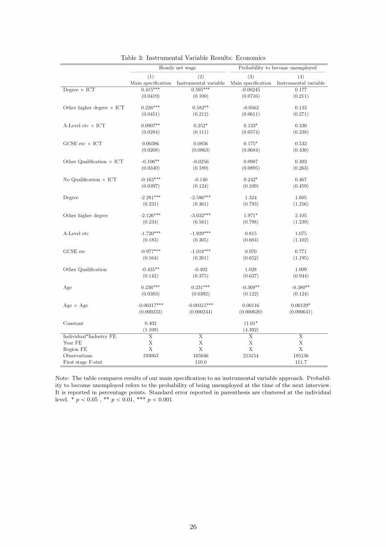
Table 3: Instrumental Variable Results: EconomicsHourly net wage Probability to become unemployed

(1) (2) (3) (4)Main specification Instrumental variable Main specification Instrumental variable

Degree ˆ ICT 0.415˚˚˚ 0.595˚˚˚ -0.00245 0.177(0.0419) (0.100) (0.0716) (0.211)

Other higher degree ˆ ICT 0.226˚˚˚ 0.582˚˚ -0.0562 0.133(0.0451) (0.212) (0.0611) (0.271)

A-Level etc ˆ ICT 0.0907˚˚ 0.252˚ 0.133˚ 0.330(0.0284) (0.111) (0.0574) (0.238)

GCSE etc ˆ ICT 0.00386 0.0856 0.175˚ 0.532(0.0208) (0.0863) (0.0684) (0.430)

Other Qualification ˆ ICT -0.106˚˚ -0.0256 0.0987 0.393(0.0340) (0.189) (0.0895) (0.263)

No Qualification ˆ ICT -0.163˚˚˚ -0.140 0.242˚ 0.467(0.0397) (0.124) (0.109) (0.459)

Degree -2.281˚˚˚ -2.586˚˚˚ 1.324 1.605(0.231) (0.361) (0.793) (1.256)

Other higher degree -2.126˚˚˚ -3.032˚˚˚ 1.971˚ 2.105(0.234) (0.561) (0.798) (1.239)

A-Level etc -1.720˚˚˚ -1.929˚˚˚ 0.815 1.075(0.183) (0.305) (0.684) (1.102)

GCSE etc -0.977˚˚˚ -1.018˚˚˚ 0.970 0.771(0.164) (0.261) (0.652) (1.195)

Other Qualification -0.435˚˚ -0.492 1.028 1.009(0.142) (0.375) (0.637) (0.944)

Age 0.236˚˚˚ 0.231˚˚˚ -0.369˚˚ -0.380˚˚

(0.0383) (0.0392) (0.122) (0.124)

Age ˆ Age -0.00317˚˚˚ -0.00315˚˚˚ 0.00116 0.00129˚

(0.000233) (0.000244) (0.000620) (0.000641)

Constant 0.402 11.01˚

(1.109) (4.392)Individual*Industry FE X X X XYear FE X X X XRegion FE X X X XObservations 193063 165046 213154 185136First stage F-stat 110.0 111.7

Note: The table compares results of our main specification to an instrumental variable approach. Probabil-ity to become unemployed refers to the probability of being unemployed at the time of the next interview.It is reported in percentage points. Standard error reported in parenthesis are clustered at the individuallevel. * p ă 0.05 , ** p ă 0.01, *** p ă 0.001

26

Table 4: Instrumental Variable Results: Political outcomesTurnout Conservatives Labour Incumbent

(1) (2) (3) (4) (5) (6) (7) (8)Main IV Main IV Main IV Main IV

Degree ˆ ICT 0.641˚ 1.550˚ 0.631˚˚ 2.264˚˚ -0.292 0.452 1.323˚˚˚ 2.496(0.256) (0.643) (0.193) (0.721) (0.204) (0.507) (0.318) (1.357)

Other higher degree ˆ ICT 0.464 2.074˚ 0.633˚˚ 1.908˚˚ -0.341 0.282 1.393˚˚ 2.492(0.346) (1.025) (0.245) (0.685) (0.215) (0.670) (0.513) (1.273)

A-Level etc ˆ ICT 0.650˚˚ 2.087˚ 0.635˚˚˚ 1.793˚˚ -0.199 -0.595 1.419˚˚˚ 2.324˚

(0.246) (0.973) (0.193) (0.609) (0.186) (0.545) (0.361) (0.914)

GCSE etc ˆ ICT 0.239 1.313 0.0239 1.332 -0.163 0.426 0.902˚˚ 2.589˚˚

(0.225) (0.931) (0.190) (0.685) (0.178) (0.641) (0.290) (0.963)

Other Qualification ˆ ICT -1.002 1.993 -0.284 1.568 -0.407 0.581 0.388 3.809(0.564) (1.777) (0.269) (0.989) (0.343) (0.940) (0.551) (1.982)

No Qualification ˆ ICT 0.0934 2.467 -0.566˚ 0.478 0.378 0.0424 0.0556 1.536(0.457) (2.973) (0.269) (1.083) (0.382) (1.423) (0.569) (1.965)

Degree -1.687 1.716 -7.278˚˚˚ -7.966˚ 3.347 0.704 -11.60˚˚˚ -10.48(3.321) (6.108) (1.877) (3.140) (2.261) (3.723) (3.513) (5.702)

Other higher degree -3.443 -2.339 -4.835˚ -4.882 1.089 -1.199 -11.25˚˚ -10.28(3.984) (6.581) (1.986) (3.162) (2.304) (3.824) (3.800) (5.683)

A-Level etc -5.841˚ -3.936 -6.151˚˚˚ -5.643˚ 1.001 1.565 -10.64˚˚˚ -9.363(2.861) (5.673) (1.715) (2.743) (2.058) (3.445) (3.108) (4.810)

GCSE etc -4.832 -2.463 -3.597˚ -3.895 1.746 -0.325 -11.38˚˚˚ -12.06˚

(2.912) (5.649) (1.684) (2.785) (1.924) (3.349) (3.144) (4.805)

Other Qualification -0.389 -1.875 -0.265 -1.796 0.0600 -3.082 -3.000 -7.958(2.275) (5.748) (1.661) (2.925) (1.789) (3.174) (2.641) (4.981)

Age -1.542˚˚ -1.494˚˚ 0.173 0.0966 0.592 0.664˚ -0.0858 -0.00582(0.481) (0.489) (0.279) (0.287) (0.327) (0.334) (0.539) (0.549)

Age ˆ Age -0.00853˚˚ -0.00913˚˚ -0.00281 -0.00218 -0.00518˚˚ -0.00577˚˚ -0.000580 -0.000336(0.00260) (0.00284) (0.00156) (0.00163) (0.00176) (0.00184) (0.00303) (0.00312)

Constant 146.5˚˚˚ 17.02 48.47˚˚˚ 68.95˚˚˚

(15.60) (9.023) (10.59) (16.70)Individual*Industry FE X X X X X X X XYear FE X X X X X X X XRegion FE X X X X X X X XObservations 108146 85517 231320 197203 231320 197203 229320 195498First stage F-stat 117.3 75.74 75.74 76.17

Note: The table compares results of our main specification to an instrumental variable approach. Column(1) and (2) compare the results for turnout, column (3) and (4) support for the Conservatives, column(5) and (6) support for Labour and column (7) and (8) support for the incumbent. All outcomes are inpercentage points . For the instrumental variable models, the first-stage F-statistic for the instrument isreported at the bottom of the table. Standard error reported in parenthesis are clustered at the individuallevel. * p ă 0.05 , ** p ă 0.01, *** p ă 0.001

All economic and political results remain qualitatively unchanged, although the instru-

mental variable approach tends to produce larger point estimates. Obtaining larger IV

estimates is not infrequent (e.g. Dasgupta, 2018) and could be due to different reasons. A

small part of the difference between our main specification and the IV is due to differences

in the sample used. As explained in section 4.2, EUKLEMS does not provide data for two

industries in the US resulting in a slightly smaller and more homogeneous sample. When

27

we rerun the main analyses on the restricted sample, the coefficients become somewhat

closer to the IV results. Measurement error may also contribute to explain the larger IV

coefficients if ICT capital stocks are better measured in a larger economy like the US.

More substantively, the difference between the coefficients suggests that our measure

of digitalization in the UK is indeed endogenous. One possible reason is that policy in

the UK may work to limit the polarizing effects of digitalization on economic and political

outcomes. Another reason could be that industrial policy in the UK might lead to an

inefficient allocation of ICT investment across industries. Yet another explanation could

be that trade unions pressure firms to mitigate the strongest symptoms of digitalization

on workers’ material and psychological well-being. All three processes would result in

attenuation bias in our main specification.

8 Robustness Checks

We run a series of additional robustness checks in order to rule out alternative interpreta-

tions and further endogeneity concerns. These tests demonstrate that our findings are not

driven by our choice of model specification and are robust to multiple modeling approaches.

The full regression tables are presented in the SI.

8.1 Placebo Test

First, we need to rule out the possibility that an increase in ICT capital stocks simply

reflects the fact that booming industries have a larger capacity to invest and offer their

workers higher wages and better conditions. If the general propensity to invest of a sector

has an effect on workers’ economic outcomes and political preferences, this could invalidate

our interpretation of our results. They would not capture the specific consequences of

digitalization but rather the effect of working in a thriving industry.

To assess this possibility, we conduct a placebo test using non-ICT capital stock per

worker as the main explanatory variable:

Non-ICT capital intensityjt “Total capital stockjt - ICT capital stockjt

(Employeesjt)

Changes in an industry’s non-ICT capital stock do not predict any of the outcomes

we are interested in. As can be seen in column (3) in the tables presented in the SI, the

28

coefficients are very small and imprecisely estimated. This was to be expected since we

argued that investment in digitalization substitutes or complements labor in a specific way

depending on their skill level. The same is not true for other kinds of capital investments

(e.g. building a new production plant or buying a new office building).

The placebo test increases our confidence in the interpretation that the main results

are driven specifically by ICT capital, since other kinds of capital do not affect workers’

political preferences in a similar way.

8.2 Excluding outliers and allowing for regional heterogeneity

One might object that our results could be driven by a few rapidly digitalizing industries.

To rule out this possibility, we excluded the three industries with the largest increase

in digitalization in recent years (Telecommunications, Mining and Quarrying and Coke,

Refined petroleum) in the models in column (4). The exclusion of these outliers does not

change results. If anything, it even increases the precision of our estimates.

Relatedly, our results could also be driven by some particularly rapidly digitalizing

regions such as the metropolitan area of London. To account for this, we interact the

time fixed effects with regional dummies. Column (5) in the tables presented in the SI

confirms that the results are not driven by these regions, as point estimates remain largely

unchanged for all outcomes while standard errors decrease for some outcomes.

8.3 Including more workers who may have been displaced by technology

Another key concern is that our models are too restrictive towards losers and thus may

underestimate the effects of digitalization because they miss the negative effects on workers

who are displaced by digitalization and do not work in the same industry in the next period

when they are re-interviewed. This could happen for two different reasons. If displaced

workers drop out of the labor force they would not be assigned to an industry in the

next interview and would therefore drop out of our analysis. If they switch to a different

industry, the industry-spell fixed effects would absorb part of the effect of job displacement

on economic and political outcomes. In any case, our models may fail to capture the effects

of digitalization on some displaced workers workers.

We deal with this concern by relaxing the sample restriction in two ways and thus

potentially capturing more losers: First, we replicate all analyses using lead models in

29

which we examine how our measure of digitalization affects labor market and political

outcomes measured at the time of the next interview. In this way, we keep in our sample

all workers who may have been displaced by digitalization (and either exit the labor force or

work in a different industry). This results in a slightly smaller sample, but the coefficients

reported in column (6) confirm that the results remain unchanged when using leads. The

only exception is voter turnout, as several of the coefficients of interest become statistically

non-significant.

Second, we replicate all analyses using a unique individual fixed effect by respondent

instead of industry-spell fixed effects. Using this approach, workers who change industries

(perhaps in response to job displacement due to technology) contribute to the average

estimates of the effect of digitalization on labor market and political outcomes, although

workers who drop out of the labor force entirely are still excluded from the sample. The

results are reported in column (7) in the tables in the SI. Although the polarizing effect of

digitalization on wages is still clearly visible, this specification results in smaller estimates

of the effects of digitalization on hourly pay for both highly and less educated workers. This

was to be expected as using unique individual fixed effects adds large measurement error

to our treatment variable which causes attenuation bias in the estimated coefficients.21

An alternative explanation is that economic benefits of digitalization are reaped mostly by

educated workers who stay in their industries while the costs may be borne also by less

educated workers who choose to stay in the same industries. Using this specification, we

do not find effects of digitalization on voter turnout, but we still observe that digitalization

is associated with increased support for the Conservatives and the incumbent party among

workers with more education.

8.4 Including controls for trade

A possible threat to identification is that our indicator of technology may be correlated

with changes in international trade in an industry. In that case, our estimates would

partially capture effects of international trade on economic outcomes and political behavior.

However, previous work on the geography of trade shocks and technological change in the21The variation in digitalization created by industry switches is much larger than the year to year

variation for stayers which is problematic for two reasons. First, frequent back and forth switches betweentwo industries within individuals is possibly due to measurement error in the interviews. Second, wetheorize that a digitalizing workplace is what affects political attitudes, not the jumps when switchingbetween highly and low digitalized industries.

30

US shows that the two types of shocks have largely distinct distributions in space (Autor,

Dorn and Hanson, 2015), suggesting that there is limited overlap. In any case, we replicate

all the analysis controlling for international trade in the industries for which we can collect

data. Specifically, we use yearly UN Comtrade data on exports from China to the UK as

an indicators of international trade.22 This measure is only available for manufacturing

industries, resulting in a much smaller sample size. The results presented in column (8)

in the SI show that the results remain unchanged when controlling for changes in trade

within the industries for which data are available.

8.5 Panel attrition

Attrition is a concern any in panel data analysis. In our case, one may worry that digital-

ization causes differential attrition rates between winners and losers. For instance, workers

displaced by digitalization can be more likely to move and become more difficult to be

located for reinterview. In addition, as discussed above, displacement may force workers

to change industries. Higher attrition rates and more industry switches would both make

it difficult for us to capture the adverse effects of digitalization, painting an exceedingly

optimistic picture.

To examine if digitalization in an industry predicts sample attrition and industry

switches, table S10 in the SI first presents the results of regressing the likelihood of drop-

ping out of the sample or changing industries on ICT capital per worker. Next, we examine

if these effects are heterogeneous for workers with different education levels by regressing

both outcomes on the education dummies and the interaction of ICT capital per worker

and education.

The results are largely reassuring as we do not find clear evidence that ICT capital per

worker is associated with increased attrition. While the average effect of our key measure of

digitalization is in fact negative, suggesting that workers in rapidly digitalizing industries

are less likely to drop out of the panel, this difference is very small. Second, digitalization

is not clearly associated with a stronger likelihood to change to a different industry in the

next period for none of the education groups. In sum, there are some signs of attrition

in an expected direction but differences between groups are small. It thus seems unlikely

that differential attrition is driving our main results.22The data is provided for different types of goods which we first crosswalk to SIC and from there to

NACE rev. 2 codes which is used in EUKLEMS.

31

9 Discussion

The digital revolution is accompanied by two fears: that many workers will be displaced

from their jobs and that this will lead to political unrest. Public debate and the scarce

academic literature on this topic has primarily been concerned with its downsides and

focused on the losers of technological progress. While this focus is comprehensible in the

light of recent political disruptions, we contend that the imbalance in attention is at odds

with standard economic theories emphasizing productivity gains as well as with historical

experience, which has proved many gloomy projections wrong.

We document two main economic effects of digitalization. Contrary to pessimistic

accounts, a majority of workers benefit economically from rapid digitalization in their in-

dustries. Yet, these benefits are not equally distributed and they disproportionately accrue

to the highly educated. Our most novel finding is that these diverging economic trajecto-

ries are mirrored in diverging political trajectories. First of all, with respect to turnout,

we observe that digitalization reinforces inequalities along education lines: The highly

educated turn out more to vote if their sector digitalizes whereas we do not find such mo-

bilizing effects among the less educated. Second, regarding party choice, the beneficiaries

of digitalization become more likely to support the Conservative Party, in particular when

they form the government. The large but often neglected pool of voters who benefit from

technological innovation thus seems willing to support established mainstream parties and

uphold the existing social contract.

There are several substantively relevant reasons why our results seem more optimistic

about the economic and political consequences of technological change than previous work.

First of all, we look at the average effects of a general set of technologies (ICT) on the

workforce. This approach is likely to produce different results than if we had focused on the

impact of specific technologies, such as industrial robots, that may have particularly strong

displacement effects. In fact, Acemoglu and Restrepo (2017) show that industrial robots

have strong negative effects on employment and wages, whereas the effects of increases in

other ICT capital, such as computers per worker or investment in software and computers,

are often positive. Clearly, some technologies have stronger labor-displacement effects

than others. Relatedly, our approach leads us to include all sectors rather than mostly

manufacturing, a sector which has seen particularly sharp reductions in employment in

32

advanced economies, but is overall rather small.23 Our coverage of all sectors with a

more general measure of digitalization possibly facilitates identifying gains of technological

change and results in a more optimistic picture.

Another reason why our conclusions may be relatively optimistic is related to our em-

pirical approach. We deliberately study the political implications of digitalization on the

active labor force, not on the population as a whole, and we study individual effects, which

can differ from contextual effects. Using a longitudinal approach, we find little indication of

political disruption but rather business as usual. We do not include in our sample retired

or disabled people, students or people doing housework, even though workplace digital-

ization may affect them through various channels including the changes in communities

and spillovers within the household. Some segments of this population might react more

negatively, e.g. workers who lose their job and cannot find a new one or young citizens

with troubles entering the labor market in the first place, although the size of these groups

is too small to produce large differences. Finally, contextual effects can operate even on

people in the labor force in ways that are not captured by our empirical approach. For

these reasons, we do not make inferences based on our findings to population-wide political

effects.

To conclude, our findings reveal a complex and presumably more realistic picture of the

political consequences of technological change. The innovative empirical analysis provides

abundant and robust evidence that digitalization is economically beneficial for a majority

of the labor force. And it is politically consequential in two contrasting ways: First, the

large group of winners become more likely to support incumbent mainstream parties and

thus can act as a stabilizing force in democratic systems. Second, while we do not find

evidence of an anti-establishment backlash as a reaction to digitalization, we demonstrate

that the economic polarization associated with digitalization is accompanied by differential

political effects on winners and losers of this process. The resulting divergence in political

behavior between the two groups could translate quite directly into increasing political

polarization. All in all, however, the implications of digitalization at the workplace are

more multi-faceted than the simple narrative of the "revenge of the left-behind" suggests.23In the US, the workforce in the manufacturing sector has never exceeded 20% in the post-war period

and currently represents less than 13%, a figure that according to the Office for National Statistics standsbelow 10% in the UK.

33

References

Acemoglu, Daron and Pascual Restrepo. 2017. “Robots and Jobs: Evidence from US Labor Mar-

kets.” National Bureau of Economic Research Working Paper No. 23285.

Acemoglu, Daron and Pascual Restrepo. 2018. “Modeling Automation.” National Bureau of Eco-

nomic Research Working Paper No. 24321.

Arntz, Melanie, Terry Gregory and Ulrich Zierahn. 2016. The Risk of Automation for Jobs in

OECD Countries. Technical report OECD Social, Employment and Migration Working Papers

Nr. 189.

Autor, David, Gordon Hanson and Kaveh Majlesi. 2016. “Importing Political Polarization? The

Electoral Consequences of Rising Trade Exposure.” National Bureau of Economic Research

Working Paper No. 22637.

Autor, David H and David Dorn. 2013. “The Growth of Low-Skill Service Jobs and the Polarization

of the US Labor Market.” American Economic Review 103(5):1553–1597.

Autor, David H, David Dorn and Gordon H Hanson. 2013. “The China Syndrome: Local La-

bor Market Effects of Import Competition in the United States.” American Economic Review

103(6):2121–2168.

Autor, David H., David Dorn and Gordon H. Hanson. 2015. “Untangling Trade and Technology:

Evidence from Local Labour Markets.” The Economic Journal 125(584):621–646.

Autor, David H., Frank Levy and Richard J. Murnane. 2003. “The Skill Content of Recent Techno-

logical Change: An Empirical Exploration.” The Quarterly Journal of Economics pp. 1279–1333.

Autor, David H., Lawrence F. Katz and Melissa S. Kearney. 2006. “The polarization of the US

labor market.” The American economic review 96(2):189–194.

Aytaç, S. Erdem, Eli Gavin Rau and Susan Stokes. 2018. “Beyond Opportunity Costs: Campaign

Messages, Anger and Turnout among the Unemployed.” British Journal of Political Science

pp. 1–15.

Berman, E., J. Bound and S. Machin. 1998. “Implications of skill-biased technological change:

International evidence.” The Quarterly Journal of Economics 113(4):1245–1279.

Boix, Carles. 2015. Political Order and Inequality. Cambridge, MA: Cambridge University Press.

Brambor, Thomas, William R. Clark and Matt Golder. 2006. “Understanding Interaction Models:

Improving Empirical Analyses.” Political Analysis 14(1):63–82.

Broockman, David, Greg Ferenstein and Neil A. Malhotra. 2017. “Wealthy Elites’ Policy Pref-

erences and Economic Inequality: The Case of Technology Entrepreneurs.” SSRN Electronic

Journal .

Buck, Nick and Stephanie McFall. 2011. “Understanding Society: Design Overview.” Longitudinal

and Life Course Studies 3(1):5–17.

34

Caprettini, Bruno and Hans-Joachim Voth. 2017. “Rage Against the Machines: Labour-Saving

Technology and Unrest in England, 1830-32.” SSRN Working paper .

Clarke, Harold D., David Sanders, Marianne C. Stewart and Paul Whiteley. 2004. Political Choice

in Britain. Oxford: Oxford University Press.

Colantone, Italo and Piero Stanig. 2018a. “Global Competition and Brexit.” American Political

Science Review 112(2):201–218.

Colantone, Italo and Piero Stanig. 2018b. “The Trade Origins of Economic Nationalism: Import

Competition and Voting Behavior in Western Europe.” American Journal of Political Science

62(4):936–953.

Cortes, Guido Matias. 2016. “Where have the middle-wage workers gone? A study of polarization

using panel data.” Journal of Labor Economics 34(1):63–105.

Dal Bó, Ernesto, Frederico Finan, Olle Folke, Torsten Persson and Johanna Rickne. 2018. “Eco-

nomic Losers and Political Winners: Sweden’s Radical Right.” Manuscript p. 61.

Dalton, Russell J. 2017. The Participation Gap: Social Status and Political Inequality. Oxford:

Oxford University Press.

Dasgupta, Aditya. 2018. “Technological Change and Political Turnover: The Democratizing Effects

of the Green Revolution in India.” American Political Science Review 918-938(4):918–938.

Dauth, Wolfgang, Sebastian Findeisen, Jens Südekum and Nicole Wössner. 2017. German Robots

– The Impact of Industrial Robots on Workers. Technical report IAB Discussion Paper Nr. 30.

Edsall, Thomas B. 2018. “Opinion | Robots Can’t Vote, but They Helped Elect Trump.” The New

York Times .

Emmenegger, Patrick, Paul Marx and Dominik Schraff. 2017. “Off to a bad start: Unemployment

and political interest during early adulthood.” The Journal of Politics 79(1):315–328.

Evans, Geoffrey and James Tilley. 2017. The New Politics of Class: The Political Exclusion of the

British Working Class. Oxford, New York: Oxford University Press.

Fiorina, Morris P. 1978. “Economic retrospective voting in American national elections: A micro-

analysis.” American Journal of Political Science pp. 426–443.

Frey, Carl Benedikt and Michael A. Osborne. 2017. “The future of employment: How susceptible

are jobs to computerisation?” Technological Forecasting and Social Change 114:254–280.

Frey, Carl Benedikt, Thor Berger and Chinchih Chen. 2018. “Political machinery: did robots swing

the 2016 US presidential election?” Oxford Review of Economic Policy 34(3):418–442.

Goldin, Claudia Dale and Lawrence F. Katz. 2009. The Race between Education and Technology.

Harvard University Press. Google-Books-ID: yGlCFqnakCoC.

Goos, Maarten, Alan Manning and Anna Salomons. 2009. “Job polarization in Europe.” The

American Economic Review 99(2):58–63.

Goos, Maarten, Alan Manning and Anna Salomons. 2014. “Explaining Job Polarization: Routine-

35

Biased Technological Change and Offshoring.” The American Economic Review 104(8):2509–

2526.

Graetz, Georg and Guy Michaels. 2015. Robots at Work. Technical Report ID 2589780 Social

Science Research Network.

Hardy, Wojciech, Roma Keister and Piotr Lewandowski. 2018. “Educational upgrading, structural

change and the task composition of jobs in Europe.” Economics of Transition 26(2):201–231.

Heath, Oliver. 2016. “Policy alienation, social alienation and working-class abstention in Britain,

1964–2010.” British Journal of Political Science pp. 1–21.

Hershbein, Brad and Lisa B. Kahn. 2018. “Do Recessions Accelerate Routine-Biased Technological

Change? Evidence from Vacancy Postings.” American Economic Review 108(7):1737–1772.

Iversen, T. and D. Soskice. 2006. “Electoral institutions and the politics of coalitions: Why some

democracies redistribute more than others.” American Political Science Review 100(2):165–181.

Iversen, Torben and David Soskice. 2019. Democracy and Prosperity Reinventing Capitalism

through a Turbulent Century. Princeton University Press.

Jaeger, Kirsten. 2017. “EU KLEMS Growth and Productivity Accounts September 2017 Release.”

Description of Methodology and General Notes.

Jaumotte, Florence, Subir Lall and Chris Papageorgiou. 2013. “Rising Income Inequality: Tech-

nology, or Trade and Financial Globalization?” IMF Economic Review 61(2):271–309.

Jensen, J. Bradford, Dennis P. Quinn and Stephen Weymouth. 2017. “Winners and Losers in

International Trade: The Effects on US Presidential Voting.” International Organization pp. 1–

35.

Kurer, Thomas and Aina Gallego. 2018. “Distributional Consequences of Technological Change:

Worker-Level Evidence.” Manuscript. .

Lewis-Beck, Michael S. and Mary Stegmaier. 2000. “Economic determinants of electoral outcomes.”

Annual Review of Political Science 3(1):183–219.

Margalit, Yotam. 2011. “Costly Jobs: Trade-related Layoffs, Government Compensation, and

Voting in US Elections.” American Political Science Review 105(1):166–188.

Margalit, Yotam. 2013. “Explaining social policy preferences: Evidence from the Great Recession.”

American Political Science Review 107(01):80–103.

Marx, Paul and Christoph Nguyen. 2016. “Are the Unemployed Less Politically Involved? A

Comparative Study of Internal Political Efficacy.” European Sociological Review 32(5):634–648.

Michaels, Guy, Ashwini Natraj and John Van Reenen. 2014. “Has ICT Polarized Skill Demand?

Evidence from Eleven Countries over Twenty-Five Years.” Review of Economics and Statistics

96(1):60–77.

Mokyr, Joel. 2018. “The Past and the Future of Innovation: some lessons from Economic History.”

Economics of Artificial Intelligence 69:13–26.

36

Mokyr, Joel, Chris Vickers and Nicolas L. Ziebarth. 2015. “The History of Technological Anxi-

ety and the Future of Economic Growth: Is this Time Different?” The Journal of Economic

Perspectives 29(3):31–50.

O’Mahony, Mary and Marcel P. Timmer. 2009. “Output, input and productivity measures at the

industry level: the EU KLEMS database.” The Economic Journal 119(538):F374–F403.

Rehm, Philipp, Jacob S. Hacker and Mark Schlesinger. 2012. “Insecure alliances: Risk, inequality,

and support for the welfare state.” American Political Science Review 106(02):386–406.

Rosenstone, Steven J. 1982. “Economic adversity and voter turnout.” American Journal of Political

Science pp. 25–46.

Rovny, Allison E. and Jan Rovny. 2017. “Outsiders at the ballot box: operationalizations and

political consequences of the insider–outsider dualism.” Socio-Economic Review .

Rueda, David. 2005. “Insider–outsider politics in industrialized democracies: the challenge to social

democratic parties.” American Political Science Review 99(01):61–74.

Smets, Kaat and Carolien Van Ham. 2013. “The embarrassment of riches? A meta-analysis of

individual-level research on voter turnout.” Electoral Studies 32(2):344–359.

Thewissen, Stefan and David Rueda. 2017. “Automation and the Welfare State: Technological

Change as a Determinant of Redistribution Preferences.” Comparative Political Studies p. online

first.

Tilley, James, Anja Neundorf and Sara B. Hobolt. 2018. “When the Pound in People’s Pocket

Matters: How Changes to Personal Financial Circumstances Affect Party Choice.” The Journal

of Politics 80(2):555–569.

Verba, Sidney, Kay Lehman Schlozman and Henry E. Brady. 1995. Voice and equality: civic

voluntarism in American politics. Cambridge, Mass.: Harvard University Press.

37

SUPPORTING INFORMATION

Part

Table of Contents

S1 Description of the data i

S2 Crosswalking and Merging Data Sets vi

S3 Comparison of RTI and education as key dimension vii

S4 Economic Effects Before and After the 2010 Government Change ix

S5 Robustness checks: Full tables x

S6 Other political outcomes xvii

S7 Attrition xx

S8 Alternative Clustering xxi

S1 Description of the data

This section presents the longitudinal evolution of our dependent variables between 1997

and 2015, dividing the sample by education level. Figure S1 plots the average net hourly

wage. As in the main analysis, we use constant 2010 prices. The wages of all educational

groups have increased over time. In the period until the financial crisis, the growth was

largely similar for all income groups, but there is a divergence after the crisis between

respondents with university degrees and the rest.

i

Figure S1: Average hourly net wage by education

3

6

9

12

15

2000 2005 2010 2015

Year

Ave

rage H

ourl

y W

age in G

BP

Education level

Degree

Other higher degree

A−Level etc

GCSE etc

Other Qualification

No Qualification

Note: Hourly net wage calculated as monthly net wage in constant 2010 prices normalized by average hour

worked. Workers with less than half time employment (<20h) excluded. In 2009, BHPS is changed into

US which results in the inclusion of new households into the sample.

Figure S2 presents the percentage of respondents who were unemployed in the week

when the interview was conducted. Here again we observe some divergence, as increases in

unemployment after the crisis were particularly visible among citizens with less education.

Note that unemployment shares in our actual sample are smaller because those who stay

unemployed for two periods are not captured by our operationalization.

ii

Figure S2: Share unemployed by education

5%

10%

15%

2000 2005 2010 2015

Year

Share

of unem

plo

yed Education level

No Qualification

Other Qualification

GCSE etc

A−Level etc

Other higher degree

Degree

Note: Share unemployed at the time of the interview.

Figure S3 describes the probability to become unemployed (i.e. to be unemployed at

the time of next interview). Again, we see that less educated respondents are more likely

to become unemployed and there is an increase after the financial crisis of 2008.

iii

Figure S3: Probability to become unemployed in the next period by education

1%

2%

3%

4%

5%

2000 2005 2010 2015

Year

Pro

babili

ty to b

ecom

e u

nem

plo

yed

Education level

No Qualification

Other Qualification

GCSE etc

A−Level etc

Other higher degree

Degree

Note: Average probability to become unemployed in the next interview for different education groups.Currently unemployed and respondents without any industry assignment are excluded to ensure equivalencewith the main analysis. In 2009, BHPS is changed into US which results in the inclusion of new householdsinto the sample.

Figure S4 plots reported turnout for different education levels. Note that this was only

asked infrequently after 2008. There was a steady decline in turnout until the mid 2000s

and then a partial recovery. Turnout is consistently higher for the highly educated.

Figure S4: Reported voter turnout by education

A−Level etc Other higher degree Degree

No Qualification Other Qualification GCSE etc

2000 2005 2010 2015 2000 2005 2010 2015 2000 2005 2010 2015

60%

70%

80%

60%

70%

80%

Year

Turn

out

Note: Participation in elections was asked in all waves of BHPS which ended in 2008. In the UnderstandingSociety Survey, participation in elections was only asked in 2010 and 2015.

Figure S5 plots the average support for the political parties included in the analyses:

iv

the Conservative Party, the Labour Party, as well as the Liberal-Democratic Party, and

UKIP (since 2013). We observe a markedly different evolution of support for parties for

different education groups, with support for the Conservatives having grown most among

workers with university degrees, at the expense of the Liberal-Democratic Party. Some of

the time trends will be captured by the year fixed effects.

Figure S5: Support for political parties by education

A−Level etc Other higher degree Degree

No Qualification Other Qualification GCSE etc

2000 2005 2010 2015 2000 2005 2010 2015 2000 2005 2010 2015

0%

10%

20%

30%

0%

10%

20%

30%

Year

Vote

share

Conservatives Labour LibDem UKIP

Note: Vote shares calculated based on sample responses answering they voted for the respective partydivided by the number of responses for any party including other parties not reported here.

v

S2 Crosswalking and Merging Data Sets

The BHPS, UKHLS and the EU KLEMS datasets are provided using different classifi-

cations, which we address by constructing cross-walks. We are able to match the 2007

version of the Standard Industrial Classification (SIC07), used between 2009 and 2015

comprehensively to the classification scheme used by EU KLEMS (NACE Rev. 2). We

also manually construct cross-walks from SIC 1992, used in 1994, 1997 and from 2001 to

2008, and are able to match the vast majority of respondents. Between 1991 and 2001

the BHPS used the SIC 1980, which differs markedly from the following versions. We use

another crosswalk to translate SIC-80 codes into SIC-92 codes, which then allows to merge

the remaining years of EU-KLEMS data. This procedure generates an individual-level

data set with information on ICT capital per industry ranging from 1997 to 2015.

vi

S3 Comparison of RTI and education as key dimension

In this section, we show that in our panel data setting education is a stronger moderator

than RTI at predicting if workers stand to gain or lose from workplace digitalization. We

created occupation-specific RTI scores from ONET data following the standard approach

of Autor and Dorn (2013), i.e. subtracting log abstract and log manual content from log

routine content of each occupation, and relying on a crosswalk by Hardy and colleagues

(2018) to merge data with European occupational codes. We then split the observations

in high and low RTI groups if they are above or below the median of RTI in the sample.

Figure S6 shows that high RTI workers in general benefit less from digitalization in

terms of wages, as we would expect, but the differences are not statistically significant.

By contrast, the strong education gradient suggests that digitalization affect highly and

less educated workers in very heterogeneous ways. We learn from this analysis that when

looking at individual trajectories, education seems to be a more important source of het-

erogeneity in the impact of digitalization than RTI. As discussed in the text, education

may be a better proxy for the ability of workers to adapt to and benefit from digitalization.

vii

Figure S6: Main outcomes split by high and low RTI

No Qualification

Other Qualification

GCSE etc

A−Level etc

Other higher degree

Degree

−.4 −.2 0 .2 .4 .6Marginal effect of digitalization (ICT/worker)

Hourly net wage

No Qualification

Other Qualification

GCSE etc

A−Level etc

Other higher degree

Degree

−.2 0 .2 .4 .6Marginal effect of digitalization (ICT/worker)

Probability to become unemployed

No Qualification

Other Qualification

GCSE etc

A−Level etc

Other higher degree

Degree

−2 −1 0 1 2Marginal effect of digitalization (ICT/worker)

Voter Turnout

No Qualification

Other Qualification

GCSE etc

A−Level etc

Other higher degree

Degree

−1 0 1Marginal effect of digitalization (ICT/worker)

Vote for Conservatives

No Qualification

Other Qualification

GCSE etc

A−Level etc

Other higher degree

Degree

−1 −.5 0 .5 1 1.5Marginal effect of digitalization (ICT/worker)

Vote for Labour

No Qualification

Other Qualification

GCSE etc

A−Level etc

Other higher degree

Degree

−1 0 1 2 3Marginal effect of digitalization (ICT/worker)

Vote for Incumbent

‚ low RTI ˛ high RTINote: Results show marginal effect of one unit increase in digitalization (1000GBP in ICT capital/worker)on hourly wage, probability to become unemployed and probability to report to have voted or support agiven political party. All results except for the hourly wage are in percentage points. High RTI and lowRTI is defined relative to the median RTI of the sample.

viii

S4 Economic Effects Before and After the 2010 Government

Change

Table S1 shows a sub-period analysis for our economic outcomes. It compares the results

for hourly net wages and the probability to become unemployed for the time before and

after the government change in 2010. The results are comparable to the composite effects.

Main difference seems to be that in the 2010 onwards period, low educated workers did

not seems to lose out in terms of wages in absolute term when they were effected by

digitalization. Nevertheless, digitalization decreased their relative wage performance as

the effect of digitalization on the wages of the higher educated increases over time.

Table S1: Economic effects pre and post Government change in May 2010Hourly Wage Unemployment

(1) (2) (3) (4)Pre May 2010 Post May 2010 Pre May 2010 Post May 2010

Degree ˆ ICT 0.338˚˚˚ 0.441˚˚˚ -0.0577 -0.0268(0.0391) (0.0546) (0.108) (0.112)

Other higher degree ˆ ICT 0.176˚˚˚ 0.279˚˚˚ -0.145 -0.154(0.0473) (0.0535) (0.0859) (0.131)

A-Level etc ˆ ICT 0.0526˚ 0.198˚˚˚ 0.203 0.170(0.0261) (0.0460) (0.107) (0.122)

GCSE etc ˆ ICT -0.0252 0.138˚˚ 0.217˚ 0.0921(0.0212) (0.0488) (0.0979) (0.152)

Other Qualification ˆ ICT -0.104˚˚ 0.0714 0.131 -0.0402(0.0359) (0.0994) (0.142) (0.213)

No Qualification ˆ ICT -0.201˚˚˚ 0.0283 0.237 0.179(0.0473) (0.0874) (0.132) (0.251)

Degree -1.439˚˚˚ -2.272˚˚˚ 3.243˚ 1.174(0.238) (0.432) (1.270) (1.954)

Other higher degree -1.437˚˚˚ -1.794˚˚˚ 4.712˚˚˚ 2.357(0.258) (0.373) (1.363) (1.792)

A-Level etc -1.196˚˚˚ -1.542˚˚˚ 1.335 0.366(0.161) (0.438) (1.010) (1.712)

GCSE etc -0.756˚˚˚ -0.673 1.627 0.894(0.163) (0.364) (1.035) (1.621)

Other Qualification -0.302˚ -0.404 1.289 2.018(0.137) (0.273) (0.868) (1.676)

Age 0.214˚˚˚ 0.305˚˚˚ -0.264 -0.152(0.0316) (0.0715) (0.169) (0.230)

Age ˆ Age -0.00299˚˚˚ -0.00428˚˚˚ -0.000129 -0.000346(0.000255) (0.000413) (0.000927) (0.00148)

Constant 0.440 3.563 4.106 7.603(1.001) (2.586) (6.523) (8.939)

Id*Ind FE X X X XYear FE X X X XRegion X X X XObservations 88960 104103 104604 108550

Note: All columns use our main specification. Column (1) and (2) report a reoport a sub-erpiod analysisfor net hourly wages (calculated as monthly net wage in constant 2010 prices normalized by average hourworked. Workers with less than half time employment (<20h) excluded). Column (3) and (4) report asub-period analysis for probability to become unemployed in percentage points (ie. to be unemployed atthe next interview conditional on currently working). Standard error reported in parenthesis are clusteredat the individual level. * p ă 0.05 , ** p ă 0.01, *** p ă 0.001

ix

S5 Robustness checks: Full tables

This section presents the tables discussed in the main text and the robustness checks.

For the sake of completeness, we also add a cross-sectional OLS regression including

only industry and year fixed effects to see how between-worker differences in ICT intensity

relate to our outcomes (column 9). Results have to be interpreted with a large grain of salt

as we now cannot control for unobserved worker-level characteristics anymore. Instead,

except for the inclusion of a gender dummy, we tried to stay as close as possible to our

main specification to ensure the comparability of results while avoiding post-treatment

bias. The results for political outcomes are surprisingly similar to the fixed-effects spec-

ification. Especially, they confirm the finding that digitalization increase support for the

Conservatives for the incumbent among highly educated workers.

Regarding economic outcomes, the results change slightly. The highly educated are

still the main beneficiaries when it comes to wages. However, looking at unemployment,

less educated people already working in digitalized industries appear to benefit from dig-

italization as they have lower probabilities to become unemployed. This is somewhat

counter-intuitive and seemingly opposite to our findings from the baseline specification.

Yet, the two diverging results make sense considering the different nature of the two anal-

yses. The cross-sectional analysis shows that working in an already digitalized industry

reduces the risk of unemployment whereas the fixed-effects specification shows that for a

given worker in a given industry, increasing digitalization might threaten the jobs of less

educated workers if tasks are automated.

x

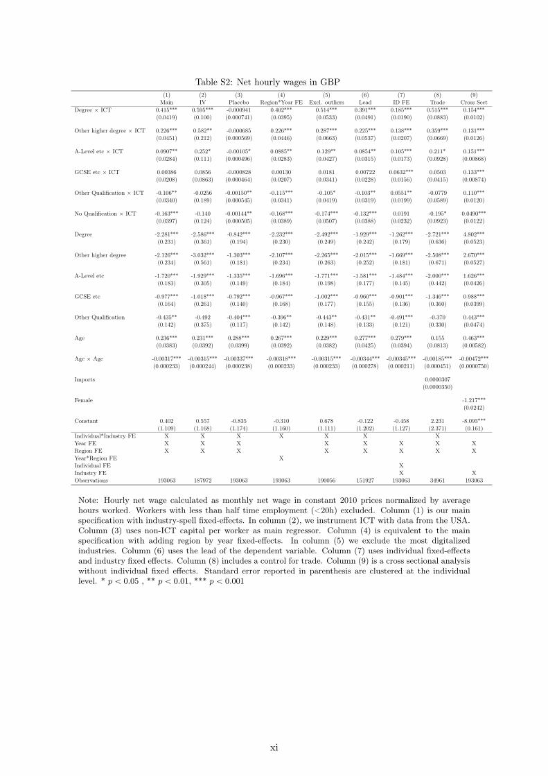
Table S2: Net hourly wages in GBP(1) (2) (3) (4) (5) (6) (7) (8) (9)Main IV Placebo Region*Year FE Excl. outliers Lead ID FE Trade Cross Sect

Degree ˆ ICT 0.415˚˚˚ 0.595˚˚˚ -0.000941 0.402˚˚˚ 0.514˚˚˚ 0.391˚˚˚ 0.185˚˚˚ 0.515˚˚˚ 0.154˚˚˚

(0.0419) (0.100) (0.000741) (0.0395) (0.0533) (0.0491) (0.0190) (0.0883) (0.0102)

Other higher degree ˆ ICT 0.226˚˚˚ 0.582˚˚ -0.000685 0.226˚˚˚ 0.287˚˚˚ 0.225˚˚˚ 0.138˚˚˚ 0.359˚˚˚ 0.131˚˚˚

(0.0451) (0.212) (0.000569) (0.0446) (0.0663) (0.0537) (0.0207) (0.0669) (0.0126)

A-Level etc ˆ ICT 0.0907˚˚ 0.252˚ -0.00105˚ 0.0885˚˚ 0.129˚˚ 0.0854˚˚ 0.105˚˚˚ 0.211˚ 0.151˚˚˚

(0.0284) (0.111) (0.000496) (0.0283) (0.0427) (0.0315) (0.0173) (0.0928) (0.00868)

GCSE etc ˆ ICT 0.00386 0.0856 -0.000828 0.00130 0.0181 0.00722 0.0632˚˚˚ 0.0503 0.133˚˚˚

(0.0208) (0.0863) (0.000464) (0.0207) (0.0341) (0.0228) (0.0156) (0.0415) (0.00874)

Other Qualification ˆ ICT -0.106˚˚ -0.0256 -0.00150˚˚ -0.115˚˚˚ -0.105˚ -0.103˚˚ 0.0551˚˚ -0.0779 0.110˚˚˚

(0.0340) (0.189) (0.000545) (0.0341) (0.0419) (0.0319) (0.0199) (0.0589) (0.0120)

No Qualification ˆ ICT -0.163˚˚˚ -0.140 -0.00144˚˚ -0.168˚˚˚ -0.174˚˚˚ -0.132˚˚˚ 0.0191 -0.195˚ 0.0490˚˚˚

(0.0397) (0.124) (0.000505) (0.0389) (0.0507) (0.0388) (0.0232) (0.0923) (0.0122)

Degree -2.281˚˚˚ -2.586˚˚˚ -0.842˚˚˚ -2.232˚˚˚ -2.492˚˚˚ -1.929˚˚˚ -1.262˚˚˚ -2.721˚˚˚ 4.802˚˚˚

(0.231) (0.361) (0.194) (0.230) (0.249) (0.242) (0.179) (0.636) (0.0523)

Other higher degree -2.126˚˚˚ -3.032˚˚˚ -1.303˚˚˚ -2.107˚˚˚ -2.265˚˚˚ -2.015˚˚˚ -1.669˚˚˚ -2.508˚˚˚ 2.670˚˚˚

(0.234) (0.561) (0.181) (0.234) (0.263) (0.252) (0.181) (0.671) (0.0527)

A-Level etc -1.720˚˚˚ -1.929˚˚˚ -1.335˚˚˚ -1.696˚˚˚ -1.771˚˚˚ -1.581˚˚˚ -1.484˚˚˚ -2.000˚˚˚ 1.626˚˚˚

(0.183) (0.305) (0.149) (0.184) (0.198) (0.177) (0.145) (0.442) (0.0426)

GCSE etc -0.977˚˚˚ -1.018˚˚˚ -0.792˚˚˚ -0.967˚˚˚ -1.002˚˚˚ -0.960˚˚˚ -0.901˚˚˚ -1.346˚˚˚ 0.988˚˚˚

(0.164) (0.261) (0.140) (0.168) (0.177) (0.155) (0.136) (0.360) (0.0399)

Other Qualification -0.435˚˚ -0.492 -0.404˚˚˚ -0.396˚˚ -0.443˚˚ -0.431˚˚ -0.491˚˚˚ -0.370 0.443˚˚˚

(0.142) (0.375) (0.117) (0.142) (0.148) (0.133) (0.121) (0.330) (0.0474)

Age 0.236˚˚˚ 0.231˚˚˚ 0.288˚˚˚ 0.267˚˚˚ 0.229˚˚˚ 0.277˚˚˚ 0.279˚˚˚ 0.155 0.463˚˚˚

(0.0383) (0.0392) (0.0399) (0.0392) (0.0382) (0.0425) (0.0394) (0.0813) (0.00582)

Age ˆ Age -0.00317˚˚˚ -0.00315˚˚˚ -0.00337˚˚˚ -0.00318˚˚˚ -0.00315˚˚˚ -0.00344˚˚˚ -0.00345˚˚˚ -0.00185˚˚˚ -0.00472˚˚˚

(0.000233) (0.000244) (0.000238) (0.000233) (0.000233) (0.000278) (0.000211) (0.000451) (0.0000750)

Imports 0.0000307(0.0000350)

Female -1.217˚˚˚

(0.0242)

Constant 0.402 0.557 -0.835 -0.310 0.678 -0.122 -0.458 2.231 -8.093˚˚˚

(1.109) (1.168) (1.174) (1.160) (1.111) (1.202) (1.127) (2.371) (0.161)Individual*Industry FE X X X X X X XYear FE X X X X X X X XRegion FE X X X X X X X XYear*Region FE XIndividual FE XIndustry FE X XObservations 193063 187972 193063 193063 190056 151927 193063 34961 193063

Note: Hourly net wage calculated as monthly net wage in constant 2010 prices normalized by averagehours worked. Workers with less than half time employment (<20h) excluded. Column (1) is our mainspecification with industry-spell fixed-effects. In column (2), we instrument ICT with data from the USA.Column (3) uses non-ICT capital per worker as main regressor. Column (4) is equivalent to the mainspecification with adding region by year fixed-effects. In column (5) we exclude the most digitalizedindustries. Column (6) uses the lead of the dependent variable. Column (7) uses individual fixed-effectsand industry fixed effects. Column (8) includes a control for trade. Column (9) is a cross sectional analysiswithout individual fixed effects. Standard error reported in parenthesis are clustered at the individuallevel. * p ă 0.05 , ** p ă 0.01, *** p ă 0.001

xi

Table S3: Probability to become unemployed(1) (2) (3) (4) (5) (6) (7) (8) (9)Main IV Placebo Region*Year FE Excl. outliers Lead ID FE Trade Cross Sect

Degree ˆ ICT -0.00245 0.177 0.00000172 -0.000390 -0.0930 0.130 0.0531 -0.169 0.0118(0.0716) (0.211) (0.000685) (0.0715) (0.0794) (0.114) (0.0455) (0.0997) (0.0247)

Other higher degree ˆ ICT -0.0562 0.133 0.000936 -0.0457 -0.157 0.00838 0.0678 -0.230 0.0217(0.0611) (0.271) (0.00101) (0.0613) (0.0899) (0.0752) (0.0748) (0.157) (0.0294)

A-Level etc ˆ ICT 0.133˚ 0.330 -0.000252 0.144˚ 0.132˚ 0.137 0.152˚˚ -0.0780 0.000546(0.0574) (0.238) (0.000901) (0.0580) (0.0656) (0.0953) (0.0518) (0.130) (0.0267)

GCSE etc ˆ ICT 0.175˚ 0.532 -0.000350 0.179˚˚ 0.165 0.254˚˚ 0.100 0.0466 -0.00449(0.0684) (0.430) (0.000748) (0.0683) (0.0908) (0.0911) (0.0511) (0.105) (0.0293)

Other Qualification ˆ ICT 0.0987 0.393 -0.000299 0.0988 0.0159 0.102 0.0589 -0.0554 -0.00787(0.0895) (0.264) (0.00135) (0.0897) (0.0937) (0.116) (0.0886) (0.285) (0.0460)

No Qualification ˆ ICT 0.242˚ 0.467 -0.000254 0.234˚ 0.245 0.323˚ 0.0202 0.0685 -0.0671(0.109) (0.459) (0.00120) (0.109) (0.138) (0.162) (0.0857) (0.168) (0.0462)

Degree 1.324 1.605 0.608 1.309 1.591˚ 0.783 -1.854˚ 3.420 -2.234˚˚˚

(0.793) (1.256) (0.744) (0.794) (0.812) (1.005) (0.849) (1.933) (0.210)

Other higher degree 1.971˚ 2.105 1.033 1.960˚ 2.237˚˚ 2.085˚ -0.996 3.480 -1.896˚˚˚

(0.798) (1.239) (0.744) (0.796) (0.834) (1.011) (0.888) (2.722) (0.217)

A-Level etc 0.815 1.075 0.639 0.802 0.822 1.119 -0.887 1.030 -1.656˚˚˚

(0.684) (1.102) (0.634) (0.684) (0.708) (0.877) (0.753) (1.392) (0.212)

GCSE etc 0.970 0.771 0.853 0.944 1.023 1.033 -0.304 0.119 -1.092˚˚˚

(0.652) (1.195) (0.591) (0.650) (0.685) (0.841) (0.721) (1.617) (0.211)

Other Qualification 1.028 1.009 0.666 0.996 1.243 1.561˚ -0.408 1.136 -0.700˚˚

(0.637) (0.944) (0.568) (0.637) (0.650) (0.774) (0.718) (1.861) (0.257)

Age -0.369˚˚ -0.380˚˚ -0.369˚˚ -0.373˚˚ -0.380˚˚ -0.278 -0.411˚˚˚ -0.453 -0.446˚˚˚

(0.122) (0.124) (0.124) (0.124) (0.123) (0.144) (0.124) (0.332) (0.0236)

Age ˆ Age 0.00116 0.00129˚ 0.00119 0.00119 0.00106 0.00202˚˚ 0.00366˚˚˚ 0.00295 0.00467˚˚˚

(0.000620) (0.000641) (0.000619) (0.000621) (0.000623) (0.000778) (0.000621) (0.00176) (0.000273)

Imports 0.0000628(0.000120)

Female -0.498˚˚˚

(0.0740)

Constant 11.01˚ 10.77˚ 11.79˚˚ 11.40˚ 11.48˚˚ 6.936 12.61˚˚ 0.226 12.42˚˚˚

(4.392) (4.526) (4.488) (4.499) (4.427) (4.373) (4.213) (11.16) (0.627)Individual*Industry FE X X X X X X XYear FE X X X X X X X XRegion FE X X X X X X X XYear*Region FE XIndividual FE XIndustry FE X XObservations 213154 207754 213154 213154 210135 172419 213154 34645 213154

Note: Probability to become unemployed in percentage points among those currently working. Column(1) is our main specification with industry-spell fixed-effects. In column (2), we instrument ICT with datafrom the USA. Column (3) uses non-ICT capital per worker as main regressor. Column (4) is equivalentto the main specification with adding region by year fixed-effects. In column (5) we exclude the mostdigitalized industries. Column (6) uses the lead of the dependent variable. Column (7) uses individualfixed-effects and industry fixed effects. Column (8) includes a control for trade. Column (9) is a crosssectional analysis without individual fixed effects. Standard error reported in parenthesis are clustered atthe individual level. * p ă 0.05 , ** p ă 0.01, *** p ă 0.001

xii

Table S4: Voted in last general elections(1) (2) (3) (4) (5) (6) (7) (8) (9)Main IV Placebo Region*Year FE Excl. outliers Lead ID FE Trade Cross Sect

Degree ˆ ICT 0.641˚ 1.550˚ 0.00783 0.557˚ 1.035˚˚ 0.327 0.351˚ 0.339 -0.0183(0.256) (0.643) (0.00509) (0.250) (0.366) (0.277) (0.145) (0.707) (0.108)

Other higher degree ˆ ICT 0.464 2.074˚ 0.00714 0.460 0.881 0.780 0.259 0.127 -0.141(0.346) (1.025) (0.00439) (0.342) (0.537) (0.404) (0.186) (0.597) (0.129)

A-Level etc ˆ ICT 0.650˚˚ 2.087˚ 0.00632 0.661˚˚ 0.964˚˚ 1.018˚˚˚ 0.436˚˚ -0.0299 0.160(0.246) (0.974) (0.00623) (0.246) (0.353) (0.286) (0.148) (0.493) (0.114)

GCSE etc ˆ ICT 0.239 1.313 -0.00203 0.199 -0.221 0.195 0.343˚ -0.0427 0.153(0.225) (0.931) (0.00491) (0.224) (0.382) (0.248) (0.152) (0.460) (0.116)

Other Qualification ˆ ICT -1.002 1.993 -0.00527 -1.076 -0.785 -0.142 0.175 -1.922 -0.427˚

(0.564) (1.777) (0.00772) (0.563) (0.546) (0.439) (0.243) (1.158) (0.179)

No Qualification ˆ ICT 0.0934 2.467 0.00244 0.132 0.201 0.435 0.658˚ -1.306 0.297(0.457) (2.973) (0.00571) (0.455) (0.641) (0.473) (0.264) (0.787) (0.186)

Degree -1.687 1.716 -1.734 -1.462 -2.343 -3.553 -1.159 -19.36˚ 22.57˚˚˚

(3.321) (6.109) (3.242) (3.306) (3.417) (3.451) (2.861) (9.726) (0.705)

Other higher degree -3.443 -2.339 -4.107 -3.816 -4.179 -7.720 -2.900 -23.57˚ 14.91˚˚˚

(3.984) (6.582) (3.771) (3.950) (4.151) (4.082) (3.372) (11.24) (0.763)

A-Level etc -5.841˚ -3.936 -5.393˚ -5.782˚ -6.231˚ -6.129˚ -3.624 -15.15˚ 10.93˚˚˚

(2.861) (5.674) (2.727) (2.838) (2.967) (2.900) (2.508) (6.365) (0.688)

GCSE etc -4.832 -2.463 -4.564 -4.704 -3.816 -3.522 -4.726 -10.68 6.097˚˚˚

(2.912) (5.650) (2.780) (2.888) (3.057) (3.048) (2.490) (6.651) (0.679)

Other Qualification -0.389 -1.875 -2.130 -0.0428 -0.428 0.197 -1.146 4.441 2.627˚˚

(2.275) (5.749) (2.027) (2.250) (2.307) (2.370) (1.816) (5.113) (0.827)

Age -1.542˚˚ -1.494˚˚ -0.892 -0.950˚ -1.599˚˚˚ 0.604 -1.149˚˚ -1.229 1.959˚˚˚

(0.481) (0.490) (0.484) (0.484) (0.484) (0.499) (0.440) (1.152) (0.0786)

Age ˆ Age -0.00853˚˚ -0.00913˚˚ -0.00925˚˚˚ -0.00884˚˚˚ -0.00805˚˚ -0.0107˚˚˚ -0.00900˚˚˚ 0.0000360 -0.0112˚˚˚

(0.00260) (0.00284) (0.00259) (0.00259) (0.00262) (0.00266) (0.00227) (0.00632) (0.000940)

Imports -0.000504(0.000512)

Female 0.112(0.296)

Constant 146.5˚˚˚ 142.0˚˚˚ 126.6˚˚˚ 127.7˚˚˚ 148.0˚˚˚ 86.34˚˚˚ 129.4˚˚˚ 136.8˚˚˚ 14.16˚˚˚

(15.60) (16.91) (15.89) (15.91) (15.73) (17.51) (15.23) (39.14) (2.157)Individual*Industry FE X X X X X X XYear FE X X X X X X X XRegion FE X X X X X X X XYear*Region FE XIndividual FE XIndustry FE X XObservations 108146 105171 108146 108146 106403 95363 108146 19908 108146

Note: Probability to report to have voted in last general election in percentage point. Column (1) is ourmain specification with industry-spell fixed-effects. In column (2), we instrument ICT with data from theUSA. Column (3) uses non-ICT capital per worker as main regressor. Column (4) is equivalent to themain specification with adding region by year fixed-effects. In column (5) we exclude the most digitalizedindustries. Column (6) uses the lead of the dependent variable. Column (7) uses individual fixed-effectsand industry fixed effects. Column (8) includes a control for trade. Column (9) is a cross sectional analysiswithout individual fixed effects. Standard error reported in parenthesis are clustered at the individuallevel. * p ă 0.05 , ** p ă 0.01, *** p ă 0.001

xiii

Table S5: Support for the Conservative Party(1) (2) (3) (4) (5) (6) (7) (8) (9)Main IV Placebo Region*Year FE Excl. outliers Lead ID FE Trade Cross Sect

Degree ˆ ICT 0.631˚˚ 2.264˚˚ 0.00376 0.593˚˚ 0.769˚˚ 0.596˚˚ 0.424˚˚˚ 1.124 0.322˚˚˚

(0.193) (0.721) (0.00252) (0.192) (0.258) (0.201) (0.0991) (0.593) (0.0719)

Other higher degree ˆ ICT 0.633˚˚ 1.908˚˚ 0.00596˚ 0.597˚ 1.044˚˚˚ 0.719˚˚ 0.212 -0.162 0.169˚

(0.245) (0.685) (0.00294) (0.245) (0.298) (0.255) (0.125) (0.589) (0.0827)

A-Level etc ˆ ICT 0.635˚˚˚ 1.793˚˚ 0.00510 0.599˚˚ 1.147˚˚˚ 0.650˚˚˚ 0.347˚˚˚ 0.210 0.188˚

(0.193) (0.609) (0.00301) (0.190) (0.269) (0.195) (0.0998) (0.346) (0.0745)

GCSE etc ˆ ICT 0.0239 1.332 0.00176 -0.00535 0.450 0.192 0.220˚ -0.800˚ 0.261˚˚˚

(0.190) (0.685) (0.00301) (0.186) (0.250) (0.178) (0.108) (0.378) (0.0778)

Other Qualification ˆ ICT -0.284 1.568 -0.00446 -0.381 -0.143 -0.216 0.122 -0.736 -0.0524(0.269) (0.989) (0.00569) (0.277) (0.329) (0.266) (0.137) (0.516) (0.106)

No Qualification ˆ ICT -0.566˚ 0.478 -0.00194 -0.538˚ -0.580 -0.415 -0.125 -1.258 -0.196(0.269) (1.083) (0.00405) (0.268) (0.331) (0.276) (0.150) (0.842) (0.108)

Degree -7.278˚˚˚ -7.966˚ -5.339˚˚ -7.093˚˚˚ -7.235˚˚˚ -7.173˚˚˚ -5.052˚˚ -20.44˚˚˚ 8.601˚˚˚

(1.877) (3.140) (1.778) (1.881) (1.915) (1.842) (1.568) (5.861) (0.429)

Other higher degree -4.835˚ -4.882 -3.233 -4.775˚ -5.572˚˚ -7.672˚˚˚ -3.162 -4.073 11.32˚˚˚

(1.986) (3.162) (1.807) (1.981) (2.041) (2.043) (1.626) (6.528) (0.472)

A-Level etc -6.151˚˚˚ -5.643˚ -4.499˚˚ -6.066˚˚˚ -7.181˚˚˚ -8.134˚˚˚ -4.775˚˚˚ -7.242 9.454˚˚˚

(1.715) (2.744) (1.605) (1.728) (1.763) (1.629) (1.435) (3.955) (0.421)

GCSE etc -3.597˚ -3.895 -3.196˚ -3.583˚ -4.468˚˚ -5.801˚˚˚ -3.714˚˚ -0.369 7.152˚˚˚

(1.684) (2.786) (1.592) (1.694) (1.722) (1.617) (1.375) (4.527) (0.418)

Other Qualification -0.265 -1.796 0.386 0.112 -0.452 -2.407 -0.648 1.685 4.054˚˚˚

(1.661) (2.925) (1.396) (1.653) (1.706) (1.556) (1.251) (5.239) (0.509)

Age 0.173 0.0966 0.310 0.258 0.147 0.218 0.124 1.085 0.179˚˚˚

(0.279) (0.287) (0.282) (0.282) (0.282) (0.297) (0.264) (0.701) (0.0469)

Age ˆ Age -0.00281 -0.00218 -0.00313˚ -0.00264 -0.00247 -0.00591˚˚˚ -0.00153 -0.00706 0.00242˚˚˚

(0.00156) (0.00163) (0.00156) (0.00156) (0.00157) (0.00173) (0.00134) (0.00406) (0.000582)

Imports 0.000204(0.000281)

Female -0.158(0.187)

Constant 17.02 16.95 11.89 13.81 17.52 18.62 13.80 -6.264 10.30˚˚˚

(9.023) (9.497) (9.286) (9.306) (9.106) (10.00) (8.327) (21.68) (1.453)Individual*Industry FE X X X X X X XYear FE X X X X X X X XRegion FE X X X X X X X XYear*Region FE XIndividual FE XIndustry FE X XObservations 231320 225834 231320 231320 228252 191163 231320 35775 231320

Note: Probability to report to support the Conservative Party in percentage point. Column (1) is ourmain specification with industry-spell fixed-effects. In column (2), we instrument ICT with data from theUSA. Column (3) uses non-ICT capital per worker as main regressor. Column (4) is equivalent to themain specification with adding region by year fixed-effects. In column (5) we exclude the most digitalizedindustries. Column (6) uses the lead of the dependent variable. Column (7) uses individual fixed-effectsand industry fixed effects. Column (8) includes a control for trade. Column (9) is a cross sectional analysiswithout individual fixed effects. Standard error reported in parenthesis are clustered at the individual level.* p ă 0.05 , ** p ă 0.01, *** p ă 0.001

xiv

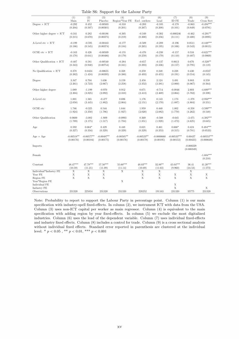
Table S6: Support for the Labour Party(1) (2) (3) (4) (5) (6) (7) (8) (9)Main IV Placebo Region*Year FE Excl. outliers Lead ID FE Trade Cross Sect

Degree ˆ ICT -0.292 0.452 -0.00503 -0.310 -0.203 -0.105 -0.178 -0.863 -0.494˚˚˚

(0.204) (0.507) (0.00301) (0.201) (0.267) (0.208) (0.101) (0.849) (0.0791)

Other higher degree ˆ ICT -0.341 0.282 -0.00186 -0.305 -0.349 -0.302 -0.000246 -0.462 -0.291˚˚

(0.215) (0.670) (0.00375) (0.219) (0.300) (0.256) (0.111) (0.400) (0.0895)

A-Level etc ˆ ICT -0.199 -0.595 -0.00443 -0.177 -0.509 -0.289 -0.196 0.0511 -0.448˚˚˚

(0.186) (0.545) (0.00374) (0.184) (0.265) (0.195) (0.106) (0.543) (0.0815)

GCSE etc ˆ ICT -0.163 0.426 -0.00509 -0.155 -0.476 -0.238 -0.157 0.534 -0.621˚˚˚

(0.178) (0.641) (0.00406) (0.179) (0.259) (0.179) (0.110) (0.487) (0.0869)

Other Qualification ˆ ICT -0.407 0.581 -0.00540 -0.384 -0.657 -0.137 0.0613 0.676 -0.328˚˚

(0.343) (0.940) (0.00754) (0.341) (0.393) (0.336) (0.157) (0.795) (0.118)

No Qualification ˆ ICT 0.378 0.0424 -0.00655 0.328 0.259 0.248 0.228 0.430 -0.0537(0.382) (1.424) (0.00395) (0.380) (0.493) (0.455) (0.191) (0.554) (0.145)

Degree 3.347 0.704 1.636 3.159 2.458 2.124 3.491 9.883 0.559(2.261) (3.723) (2.067) (2.258) (2.352) (2.381) (2.000) (6.067) (0.564)

Other higher degree 1.089 -1.199 -0.970 0.912 0.671 -0.714 -0.0846 2.603 -4.689˚˚˚

(2.304) (3.825) (2.092) (2.310) (2.413) (2.469) (2.064) (5.762) (0.598)

A-Level etc 1.001 1.565 -0.477 0.696 1.176 0.143 1.173 -1.378 -2.950˚˚˚

(2.058) (3.445) (1.882) (2.064) (2.151) (2.170) (1.887) (4.804) (0.551)

GCSE etc 1.746 -0.325 0.544 1.644 1.959 0.440 1.002 -0.358 -3.599˚˚˚

(1.924) (3.350) (1.786) (1.927) (2.020) (2.082) (1.770) (4.262) (0.548)

Other Qualification 0.0600 -3.082 -1.809 -0.0993 0.369 -0.508 -0.645 -3.475 -4.382˚˚˚

(1.789) (3.175) (1.517) (1.784) (1.851) (1.928) (1.473) (4.625) (0.645)

Age 0.592 0.664˚ 0.429 0.448 0.621 0.461 0.666˚ 0.424 0.484˚˚˚

(0.327) (0.334) (0.329) (0.329) (0.329) (0.353) (0.315) (0.781) (0.0533)

Age ˆ Age -0.00518˚˚ -0.00577˚˚ -0.00487˚˚ -0.00505˚˚ -0.00523˚˚ -0.0000660 -0.00533˚˚˚ 0.00437 -0.00553˚˚˚

(0.00176) (0.00184) (0.00175) (0.00176) (0.00178) (0.00195) (0.00153) (0.00423) (0.000649)

Imports -0.000229(0.000349)

Female -1.684˚˚˚

(0.210)

Constant 48.47˚˚˚ 47.78˚˚˚ 57.50˚˚˚ 55.60˚˚˚ 48.03˚˚˚ 32.88˚˚ 45.04˚˚˚ 36.41 41.20˚˚˚

(10.59) (11.21) (11.09) (11.14) (10.69) (11.63) (9.960) (24.53) (1.573)Individual*Industry FE X X X X X X XYear FE X X X X X X X XRegion FE X X X X X X X XYear*Region FE XIndividual FE XIndustry FE X XObservations 231320 225834 231320 231320 228252 191163 231320 35775 231320

Note: Probability to report to support the Labour Party in percentage point. Column (1) is our mainspecification with industry-spell fixed-effects. In column (2), we instrument ICT with data from the USA.Column (3) uses non-ICT capital per worker as main regressor. Column (4) is equivalent to the mainspecification with adding region by year fixed-effects. In column (5) we exclude the most digitalizedindustries. Column (6) uses the lead of the dependent variable. Column (7) uses individual fixed-effectsand industry fixed effects. Column (8) includes a control for trade. Column (9) is a cross sectional analysiswithout individual fixed effects. Standard error reported in parenthesis are clustered at the individuallevel. * p ă 0.05 , ** p ă 0.01, *** p ă 0.001

xv

Table S7: Support for the Incumbent(1) (2) (3) (4) (5) (6) (7) (8) (9)Main IV Placebo Region*Year FE Excl. outliers Lead ID FE Trade Cross Sect

Degree ˆ ICT 1.323˚˚˚ 2.496 0.0103 1.245˚˚˚ 1.957˚˚˚ 1.005˚˚ 0.968˚˚˚ 0.324 0.781˚˚˚

(0.318) (1.357) (0.00735) (0.312) (0.469) (0.363) (0.164) (0.790) (0.0808)

Other higher degree ˆ ICT 1.393˚˚ 2.492 0.00693 1.423˚˚ 2.488˚˚˚ 1.095 0.898˚˚˚ 0.434 0.792˚˚˚

(0.513) (1.273) (0.00650) (0.470) (0.557) (0.562) (0.213) (1.011) (0.0918)

A-Level etc ˆ ICT 1.419˚˚˚ 2.324˚ 0.00324 1.376˚˚˚ 2.156˚˚˚ 1.036˚ 0.885˚˚˚ -0.0190 0.672˚˚˚

(0.361) (0.914) (0.00591) (0.327) (0.418) (0.411) (0.186) (0.754) (0.0828)

GCSE etc ˆ ICT 0.902˚˚ 2.589˚˚ -0.00142 0.853˚˚ 1.479˚˚˚ 1.060˚˚ 0.712˚˚˚ -0.255 0.514˚˚˚

(0.290) (0.963) (0.00617) (0.278) (0.447) (0.332) (0.173) (0.496) (0.0876)

Other Qualification ˆ ICT 0.388 3.809 -0.00992 0.206 0.599 0.337 0.913˚˚˚ -1.386 0.662˚˚˚

(0.551) (1.982) (0.00920) (0.554) (0.664) (0.540) (0.250) (1.282) (0.119)

No Qualification ˆ ICT 0.0556 1.536 -0.0227˚ -0.0409 0.315 0.220 0.640˚ -1.051 0.284˚

(0.569) (1.965) (0.0104) (0.567) (0.745) (0.623) (0.277) (0.936) (0.138)

Degree -11.60˚˚˚ -10.48 -11.91˚˚˚ -10.63˚˚ -12.28˚˚˚ -8.791˚ -10.08˚˚˚ -17.16˚ 2.731˚˚˚

(3.513) (5.702) (3.189) (3.436) (3.725) (3.751) (2.959) (8.648) (0.542)

Other higher degree -11.25˚˚ -10.28 -10.98˚˚˚ -10.76˚˚ -13.07˚˚˚ -10.61˚˚ -9.963˚˚ -21.40˚ 2.243˚˚˚

(3.800) (5.683) (3.295) (3.659) (3.921) (4.038) (3.131) (9.780) (0.582)

A-Level etc -10.64˚˚˚ -9.363 -10.27˚˚˚ -10.19˚˚˚ -11.76˚˚˚ -8.971˚˚ -8.894˚˚ -11.96 1.493˚˚

(3.108) (4.811) (2.854) (3.051) (3.253) (3.277) (2.718) (6.705) (0.533)

GCSE etc -11.38˚˚˚ -12.06˚ -11.90˚˚˚ -11.22˚˚˚ -11.89˚˚˚ -11.74˚˚˚ -11.86˚˚˚ -16.31˚˚ 0.335(3.144) (4.806) (2.845) (3.052) (3.331) (3.331) (2.710) (6.275) (0.530)

Other Qualification -3.000 -7.958 -4.544˚ -3.135 -2.648 -2.978 -3.390 1.166 -1.746˚˚

(2.641) (4.981) (2.274) (2.602) (2.740) (2.758) (2.168) (6.341) (0.630)

Age -0.0858 -0.00582 -0.0488 -0.159 -0.191 -0.660 -0.0591 -1.879 0.556˚˚˚

(0.539) (0.549) (0.528) (0.529) (0.542) (0.546) (0.538) (1.341) (0.0518)

Age ˆ Age -0.000580 -0.000336 -0.00138 -0.000436 0.000221 -0.00135 -0.0000848 -0.00449 -0.00411˚˚˚

(0.00303) (0.00312) (0.00295) (0.00296) (0.00305) (0.00349) (0.00268) (0.00791) (0.000636)

Imports -0.00163˚

(0.000640)

Female -0.298(0.204)

Constant 68.95˚˚˚ 64.55˚˚˚ 86.60˚˚˚ 86.77˚˚˚ 71.55˚˚˚ 67.88˚˚˚ 66.78˚˚˚ 120.1˚˚ 34.85˚˚˚

(16.70) (17.49) (17.32) (17.36) (16.86) (17.16) (16.88) (40.17) (1.613)Individual*Industry FE X X X X X X XYear FE X X X X X X X XRegion FE X X X X X X X XYear*Region FE XIndividual FE XIndustry FE X XObservations 229320 223879 229320 229320 226288 189965 229320 35482 229320

Note: Probability to report to support the incumbent in percentage point. Until May 2010, Labour iscoded as the incumbent whereas the Conservatives after 2010. Column (1) is our main specification withindustry-spell fixed-effects. In column (2), we instrument ICT with data from the USA. Column (3) usesnon-ICT capital per worker as main regressor. Column (4) is equivalent to the main specification withadding region by year fixed-effects. In column (5) we exclude the most digitalized industries. Column(6) uses the lead of the dependent variable. Column (7) uses individual fixed-effects and industry fixedeffects. Column (8) includes a control for trade. Column (9) is a cross sectional analysis without individualfixed effects. Standard error reported in parenthesis are clustered at the individual level. * p ă 0.05 , **p ă 0.01, *** p ă 0.001

xvi

S6 Other political outcomes

The following tables report the results of additional analyses examining if digitalization

affects support for the Liberal Democratic Party and UKIP.

First, we do not find a change in the support for the Liberal Democratic Party among

workers who experience digitalization. The Liberal Democratic Party is a centrist party,

that includes both classical economic liberals as well as social-democrats. The two main

wings have varying strengths across constituencies and over time. One possible interpre-

tation of this finding is that these different factions within the party cancel each other

out. It is furthermore noteworthy that it seems that Libdem could not capitalize from an

incumbency advantage.

Second, we find some tentative evidence for increased UKIP support (only asked since

2013) among the lowest qualified respondents in our sample, which would be consistent with

the possibility that digitalization makes losers more likely to support anti-establishment

parties, in this case from the radical right. Among workers with no formal qualification,

an increase in ICT intensity produces a substantively large increase in the likelihood to

support UKIP. However, the point estimates are never significant . Furthermore, the results

have to be interpreted with caution since they are based on a relatively small sample and

a very short period of time, as the option to report support for the UKIP is only provided

in the latest three waves of the Understanding Society survey.

xvii

Table S8: Support for the Liberal Democratic Party(1) (2) (3) (4) (5) (6) (7) (8) (9)Main IV Placebo Region*Year FE Excl. outliers Lead ID FE Trade Cross Sect

Degree ˆ ICT -0.0489 -1.650˚ -0.00213 -0.0511 -0.0975 -0.0914 -0.0850 -0.656 0.165˚˚

(0.132) (0.656) (0.00217) (0.132) (0.204) (0.159) (0.0753) (0.403) (0.0527)

Other higher degree ˆ ICT 0.0557 -0.934 -0.00173 0.0700 0.0293 -0.0600 -0.104 -0.0856 0.0666(0.172) (0.648) (0.00258) (0.171) (0.251) (0.202) (0.0857) (0.377) (0.0549)

A-Level etc ˆ ICT 0.181 0.140 -0.000508 0.215 0.190 0.348˚˚ -0.0749 0.102 0.209˚˚˚

(0.125) (0.652) (0.00206) (0.125) (0.182) (0.134) (0.0858) (0.282) (0.0521)

GCSE etc ˆ ICT 0.0646 -0.932˚ -0.00325 0.0816 0.122 0.174 0.0241 -0.0880 0.278˚˚˚

(0.129) (0.447) (0.00230) (0.130) (0.195) (0.120) (0.0806) (0.476) (0.0561)

Other Qualification ˆ ICT 0.281 -0.527 0.00398 0.310 0.311 0.183 -0.0790 0.0760 0.216˚˚

(0.184) (0.623) (0.00469) (0.182) (0.228) (0.215) (0.139) (0.377) (0.0693)

No Qualification ˆ ICT 0.276 0.213 0.00251 0.207 0.344 -0.0184 -0.0460 0.353 0.0756(0.218) (0.796) (0.00263) (0.212) (0.288) (0.308) (0.108) (0.304) (0.0721)

Degree 3.331˚ 7.052˚˚ 2.979˚ 3.299˚ 3.762˚˚ 2.033 3.152˚˚ 5.166 9.176˚˚˚

(1.355) (2.358) (1.204) (1.356) (1.425) (1.590) (1.205) (3.340) (0.320)

Other higher degree 3.046˚ 5.208˚ 3.027˚ 2.972˚ 3.467˚ 0.849 2.812˚ 1.494 4.711˚˚˚

(1.442) (2.382) (1.299) (1.441) (1.506) (1.723) (1.320) (3.652) (0.335)

A-Level etc 2.697˚ 1.974 2.889˚˚ 2.538˚ 2.995˚ 1.069 3.614˚˚˚ 1.762 3.380˚˚˚

(1.135) (2.015) (1.008) (1.133) (1.183) (1.347) (1.053) (2.267) (0.293)

GCSE etc 1.142 3.189 1.241 0.967 1.394 0.949 1.682 -0.236 1.403˚˚˚

(1.079) (1.921) (0.949) (1.074) (1.136) (1.264) (0.997) (2.332) (0.287)

Other Qualification 0.672 2.048 0.304 0.237 0.613 0.234 1.069 3.569 0.609(1.042) (1.936) (0.901) (1.037) (1.069) (1.328) (0.909) (2.653) (0.344)

Age -0.0538 -0.0531 -0.169 -0.170 -0.0566 -0.0971 -0.174 -0.496 -0.256˚˚˚

(0.240) (0.246) (0.241) (0.241) (0.242) (0.262) (0.231) (0.566) (0.0333)

Age ˆ Age 0.00163 0.00158 0.00189 0.00188 0.00152 0.00173 0.00277˚ -0.00135 0.00382˚˚˚

(0.00128) (0.00134) (0.00128) (0.00128) (0.00129) (0.00146) (0.00115) (0.00282) (0.000409)

Imports -0.0000653(0.000215)

Female 0.868˚˚˚

(0.136)

Constant 1.249 0.978 3.936 3.769 1.143 10.88 6.149 6.717 7.421˚˚˚

(7.368) (7.668) (7.657) (7.678) (7.438) (8.267) (7.074) (18.67) (0.961)Individual*Industry FE X X X X X X XYear FE X X X X X X X XRegion FE X X X X X X X XYear*Region FE XIndividual FE XIndustry FE X XObservations 231320 225834 231320 231320 228252 191163 231320 35775 231320

Note: Probability to report to support the Liberal Democratic Party in percentage point. Column (1) isour main specification with industry-spell fixed-effects. In column (2), we instrument ICT with data fromthe USA. Column (3) uses non-ICT capital per worker as main regressor. Column (4) is equivalent to themain specification with adding region by year fixed-effects. In column (5) we exclude the most digitalizedindustries. Column (6) uses the lead of the dependent variable. Column (7) uses individual fixed-effectsand industry fixed effects. Column (8) includes a control for trade. Column (9) is a cross sectional analysiswithout individual fixed effects. Standard error reported in parenthesis are clustered at the individuallevel. * p ă 0.05 , ** p ă 0.01, *** p ă 0.001

xviii

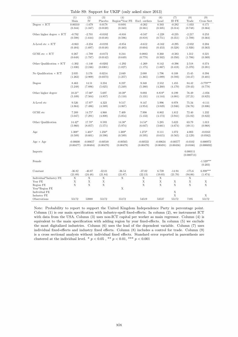
Table S9: Support for UKIP (only asked since 2013)(1) (2) (3) (4) (5) (6) (7) (8) (9)Main IV Placebo Region*Year FE Excl. outliers Lead ID FE Trade Cross Sect

Degree ˆ ICT 0.00310 -1.679 0.0178 0.0491 -0.262 0.503 -0.282 -1.033 0.171(0.344) (1.347) (0.0120) (0.343) (0.561) (0.505) (0.314) (0.748) (0.364)

Other higher degree ˆ ICT -0.792 -2.701 -0.0182 -0.816 -0.347 -1.228 -0.235 -2.217 0.253(0.598) (1.644) (0.0148) (0.596) (0.818) (0.751) (0.351) (1.709) (0.364)

A-Level etc ˆ ICT -0.863 -3.234 -0.0193 -0.854 -0.612 -0.162 -0.295 -2.832 0.204(0.484) (1.697) (0.0148) (0.483) (0.604) (0.453) (0.328) (1.926) (0.363)

GCSE etc ˆ ICT 0.267 -1.789 -0.0172 0.244 0.0883 0.260 -0.383 1.312 0.321(0.648) (1.787) (0.0142) (0.649) (0.778) (0.502) (0.350) (1.706) (0.369)

Other Qualification ˆ ICT -1.302 -1.140 -0.0202 -1.292 -1.269 0.142 -0.396 2.518 0.374(1.030) (2.246) (0.0301) (1.027) (1.175) (1.067) (0.418) (5.370) (0.381)

No Qualification ˆ ICT 2.035 3.176 0.0214 2.049 2.088 1.796 0.108 15.45 0.394(1.262) (2.909) (0.0373) (1.257) (1.365) (1.089) (0.593) (10.47) (0.401)

Degree 8.463 14.51 3.234 8.237 9.348 2.552 1.455 84.42 -3.779˚˚˚

(5.248) (7.896) (5.025) (5.249) (5.380) (4.260) (4.170) (59.43) (0.778)

Other higher degree 10.21˚ 17.00˚ 5.697 10.39˚ 9.093 8.819˚ 0.199 76.49 -1.056(5.109) (7.504) (4.857) (5.110) (5.131) (4.144) (4.081) (57.21) (0.825)

A-Level etc 9.526 17.97˚ 4.323 9.517 9.147 5.996 0.978 75.34 -0.111(4.864) (7.486) (4.569) (4.867) (4.954) (3.849) (3.946) (56.76) (0.806)

GCSE etc 7.289 14.75˚ 4.968 7.409 7.998 0.802 1.812 72.40 1.232(5.047) (7.291) (4.808) (5.054) (5.133) (4.173) (3.941) (55.82) (0.822)

Other Qualification 14.42˚ 17.78˚ 8.593 14.38˚ 14.54˚ 5.285 5.623 63.79 1.013(5.960) (8.057) (5.571) (5.974) (6.047) (3.661) (4.674) (49.11) (0.968)

Age 1.308˚ 1.401˚ 1.250˚ 1.269˚ 1.273˚ 0.111 1.072 4.003 -0.0163(0.589) (0.601) (0.590) (0.589) (0.595) (0.615) (0.565) (2.129) (0.0562)

Age ˆ Age -0.00600 -0.00657 -0.00548 -0.00565 -0.00533 -0.00634 -0.00577 -0.0102 0.000972(0.00477) (0.00484) (0.00479) (0.00479) (0.00479) (0.00491) (0.00456) (0.0166) (0.000692)

Imports 0.000111(0.000713)

Female -1.529˚˚˚

(0.203)

Constant -36.82 -40.87 -32.01 -36.54 -37.02 6.739 -14.94 -175.6 6.898˚˚˚

(21.89) (24.48) (21.84) (21.87) (22.13) (19.03) (21.70) (94.06) (1.874)Individual*Industry FE X X X X X X XYear FE X X X X X X X XRegion FE X X X X X X X XYear*Region FE XIndividual FE XIndustry FE X XObservations 55172 53988 55172 55172 54519 53537 55172 7195 55172

Note: Probability to report to support the United Kingdom Independence Party in percentage point.Column (1) is our main specification with industry-spell fixed-effects. In column (2), we instrument ICTwith data from the USA. Column (3) uses non-ICT capital per worker as main regressor. Column (4) isequivalent to the main specification with adding region by year fixed-effects. In column (5) we excludethe most digitalized industries. Column (6) uses the lead of the dependent variable. Column (7) usesindividual fixed-effects and industry fixed effects. Column (8) includes a control for trade. Column (9)is a cross sectional analysis without individual fixed effects. Standard error reported in parenthesis areclustered at the individual level. * p ă 0.05 , ** p ă 0.01, *** p ă 0.001

xix

S7 Attrition

Table S10 tests if differential attrition is a concern. We see that in general, workers who

experience digitalization are less likely to leave the sample, this effect seems to be driven at

least partially by the university educated. We never find that digitalization makes workers

more likely to leave the sample or change industry which is reassuring.

Table S10: AttritionLeave sample Change industry

(1) (2) (3) (4)

ICT -0.000553˚˚ 0.0000154(0.000169) (0.000204)

Degree ˆ ICT -0.00274˚ 0.000595(0.00131) (0.00178)

Other higher degree ˆ ICT -0.000809 -0.00147(0.00185) (0.00200)

A-Level etc ˆ ICT -0.000310 0.00106(0.00128) (0.00146)

GCSE etc ˆ ICT 0.000636 -0.0000339(0.00121) (0.00156)

Other Qualification ˆ ICT 0.000685 -0.00265(0.00247) (0.00342)

No Qualification ˆ ICT 0.00374 0.00823(0.00297) (0.00422)

Degree 0.110˚˚˚ 0.0627˚˚

(0.0174) (0.0241)

Other higher degree 0.108˚˚˚ 0.0470˚

(0.0188) (0.0235)

A-Level etc 0.0830˚˚˚ 0.00142(0.0156) (0.0207)

GCSE etc 0.0488˚˚ 0.00971(0.0155) (0.0205)

Other Qualification 0.0409˚˚ 0.0222(0.0143) (0.0193)

Age 0.0279˚˚˚ -0.0162˚˚˚

(0.00292) (0.00340)

Age ˆ Age -0.000196˚˚˚ 0.000130˚˚˚

(0.0000129) (0.0000176)

Constant 0.0538˚˚˚ -0.753˚˚˚ 0.285˚˚˚ 0.481˚˚˚

(0.00501) (0.0913) (0.00810) (0.109)Id*Ind FE X X X XYear FE X X X XRegion X X X XObservations 253814 253814 220829 220829

Note: Column (1) reports the direct effect of ICT intensity on probably to leave the sample. Column (2)reports the effect of ICT intensity on the probability to leave the sample by education group. Column (3)reports the direct effect of ICT on the probably to change industries. Column (4) reports the effect ofICT on the probably to change industries by education group. Standard error reported in parenthesis areclustered at the individual level. * p ă 0.05 , ** p ă 0.01, *** p ă 0.001

xx

S8 Alternative Clustering

Table S11 shows that our results are robust when we cluster standard errors at the industry-

year level rather than the individual level. Given that our main variable of interest is

the interaction between education (an individual-level characteristic) and digitalization (a

time-varying industry characteristic), it is not straightforward which level of clustering

is preferable. This table shows that when clustering at the industry-year level, standard

errors tend to be somewhat smaller than in the results presented in the main text.

Table S11: All outcomes with standard errors clustered at the industry-year level(1) (2) (3) (4) (5) (6)

Hourly wage Unemployed Turnout Conservative Labour IncumbentDegree ˆ ICT 0.415˚˚˚ -0.00245 0.641˚˚ 0.631˚˚˚ -0.292 1.323˚˚˚

(0.0393) (0.0919) (0.224) (0.161) (0.166) (0.385)

Other higher degree ˆ ICT 0.226˚˚˚ -0.0562 0.464 0.633˚˚ -0.341 1.393˚˚˚

(0.0371) (0.0742) (0.340) (0.208) (0.189) (0.393)

A-Level etc ˆ ICT 0.0907˚˚˚ 0.133 0.650˚ 0.635˚˚˚ -0.199 1.419˚˚˚

(0.0218) (0.0725) (0.259) (0.163) (0.157) (0.340)

GCSE etc ˆ ICT 0.00386 0.175˚ 0.239 0.0239 -0.163 0.902˚˚˚

(0.0183) (0.0860) (0.279) (0.186) (0.176) (0.267)

Other Qualification ˆ ICT -0.106˚˚˚ 0.0987 -1.002 -0.284 -0.407 0.388(0.0313) (0.104) (0.573) (0.236) (0.347) (0.429)

No Qualification ˆ ICT -0.163˚˚˚ 0.242˚ 0.0934 -0.566˚ 0.378 0.0556(0.0370) (0.103) (0.499) (0.225) (0.313) (0.426)

Degree -2.281˚˚˚ 1.324 -1.687 -7.278˚˚˚ 3.347 -11.60˚˚˚

(0.257) (0.852) (3.246) (1.833) (2.066) (3.153)

Other higher degree -2.126˚˚˚ 1.971˚ -3.443 -4.835˚ 1.089 -11.25˚˚˚

(0.220) (0.881) (3.823) (1.889) (2.168) (3.005)

A-Level etc -1.720˚˚˚ 0.815 -5.841˚ -6.151˚˚˚ 1.001 -10.64˚˚˚

(0.157) (0.702) (2.931) (1.589) (1.832) (2.529)

GCSE etc -0.977˚˚˚ 0.970 -4.832 -3.597˚ 1.746 -11.38˚˚˚

(0.116) (0.703) (2.913) (1.547) (1.959) (2.514)

Other Qualification -0.435˚˚˚ 1.028 -0.389 -0.265 0.0600 -3.000(0.123) (0.687) (2.537) (1.444) (1.701) (2.153)

Age 0.236˚˚˚ -0.369˚˚ -1.542˚˚ 0.173 0.592 -0.0858(0.0324) (0.125) (0.525) (0.291) (0.353) (0.434)

Age ˆ Age -0.00317˚˚˚ 0.00116 -0.00853˚˚ -0.00281 -0.00518˚˚ -0.000580(0.000206) (0.000696) (0.00287) (0.00146) (0.00185) (0.00201)

Constant 0.402 11.01˚ 146.5˚˚˚ 17.02˚ 48.47˚˚˚ 68.95˚˚˚

(0.946) (4.434) (17.62) (8.319) (10.08) (13.26)Individual*Industry FE X X X X X XYear FE X X X X X XRegion FE X X X X X XObservations 193063 213154 108146 231320 231320 229320

Note: All columns use the main specification. Column (1) reports the results for hourly wage, column(2) for the probability to become unemployed, column (3) for voter turnout, column (4) for vote for theConservatives, column (5) for vote for Labour and column (6) for vote for the incumbent. Standard errorreported in parenthesis are clustered at the industry-year level. * p ă 0.05 , ** p ă 0.01, *** p ă 0.001

xxi