not having the information you need when you need it...
TRANSCRIPT

Not having the information you need when you need it leaves you wanting. Not knowing where tolook for that information leaves you powerless. In a societywhere information is king, none of us
can afford that.
– Lois Horowitz.


University of Alberta
Data Mining Flow Graphs in a Dynamic Compiler
by
Adam Paul Jocksch
A thesis submitted to the Faculty of Graduate Studies and Researchin partial fulfillment of the requirements for the degree of
Master of Science
Department of Computing Science
c©Adam Paul JockschFall 2009
Edmonton, Alberta
Permission is hereby granted to the University of Alberta Libraries to reproduce single copies of this thesis and to lend orsell such copies for private, scholarly or scientific research purposes only. Where the thesis is converted to, or otherwise
made available in digital form, the University of Alberta willadvise potential users of the thesis of these terms.
The author reserves all other publication and other rights in association with the copyright in the thesis and, except ashereinbefore provided, neither the thesis nor any substantial portion thereof may be printed or otherwise reproduced in any
material form whatsoever without the author’s prior writtenpermission.


Examining Committee
Jose Nelson Amaral, Computing Science
Vincent Gaudet, Electrical and Computer Engineering
Joerg Sander, Computing Science

Abstract
This thesis introduces FlowGSP, a general-purpose sequence mining algorithm for flow graphs.
FlowGSP ranks sequences according to the frequency with which they occur and according to their
relative cost. This thesis also presents two parallel implementations of FlowGSP. The first imple-
mentation uses JavaTMthreads and is designed for use on workstations equipped with multi-core
CPUs. The second implementation is distributed in nature and intended for use on clusters.
The thesis also presents results from an application of FlowGSP to mine program profiles in
the context of the development of a dynamic optimizing compiler. Interpreting patterns within raw
profiling data is extremely difficult and heavily reliant on human intuition.
FlowGSP has been tested on performance-counter profiles collected from the IBMR©WebSphereR©
Application Server. This investigation identifies a numberof sequences which are known to be typi-
cal of WebSphereR© Application Server behavior, as well as some sequences which were previously
unknown.


Acknowledgements
I would like to thank my supervisor Nelson, first and foremost, for his endless support, encourage-
ment, and especially for his patience.
I would like to thank Osmar Zaıne for his advice in the planning stages of my research. His
advice on existing data mining algorithms was invaluable.
I would also like to thank the IBM Testarossa JIT developmentteam, specifically Marcel Mitran,
Joran Siu, and Nikola Grcevski. They have provided me with anabundance of technical information
and guidance throughout my research.
The research leading up to this thesis was made possible by funding from the IBM Center for
Advanced Studies (CAS) and by grants from the Natural Science and Engineering Research Council.

Contents
1 Introduction 3
2 Background Information 72.1 Machine Learning . . . . . . . . . . . . . . . . . . . . . . . . . . . . . . . . .. . 7
2.1.1 Data Mining . . . . . . . . . . . . . . . . . . . . . . . . . . . . . . . . . 82.1.2 Frequent-Sequence Mining . . . . . . . . . . . . . . . . . . . . . . .. . . 92.1.3 GSP . . . . . . . . . . . . . . . . . . . . . . . . . . . . . . . . . . . . . . 9
2.2 Compiler Technology . . . . . . . . . . . . . . . . . . . . . . . . . . . . . .. . . 102.2.1 Control Flow Graphs (CFGs) . . . . . . . . . . . . . . . . . . . . . . .. . 102.2.2 Edge Profiling vs. Path Profiling . . . . . . . . . . . . . . . . . . .. . . . 112.2.3 Dynamic Optimization . . . . . . . . . . . . . . . . . . . . . . . . . . .. 12
2.3 Performance Counters . . . . . . . . . . . . . . . . . . . . . . . . . . . . .. . . 142.4 z10 Architecture . . . . . . . . . . . . . . . . . . . . . . . . . . . . . . . . .. . . 15
2.4.1 Address Generation Interlock . . . . . . . . . . . . . . . . . . . .. . . . 152.4.2 Page Sizes . . . . . . . . . . . . . . . . . . . . . . . . . . . . . . . . . . 152.4.3 Performance Counters on z10 . . . . . . . . . . . . . . . . . . . . . .. . 16
2.5 WebSphere Application Server . . . . . . . . . . . . . . . . . . . . . .. . . . . . 162.5.1 Profiling WAS . . . . . . . . . . . . . . . . . . . . . . . . . . . . . . . . 17
2.6 Parallel Performance . . . . . . . . . . . . . . . . . . . . . . . . . . . . .. . . . 172.6.1 Linear Speedup . . . . . . . . . . . . . . . . . . . . . . . . . . . . . . . . 172.6.2 Memory Organization . . . . . . . . . . . . . . . . . . . . . . . . . . . .18
3 FlowGSP 213.1 Edge and Vertex Weighted Attributed Flow Graphs . . . . . . .. . . . . . . . . . 22
3.1.1 Formal Definition . . . . . . . . . . . . . . . . . . . . . . . . . . . . . . .223.2 Calculating Path Support . . . . . . . . . . . . . . . . . . . . . . . . . .. . . . . 24
3.2.1 Frequency Support . . . . . . . . . . . . . . . . . . . . . . . . . . . . . .243.2.2 Weight Support . . . . . . . . . . . . . . . . . . . . . . . . . . . . . . . . 25
3.3 Sequences of Attributes . . . . . . . . . . . . . . . . . . . . . . . . . . .. . . . . 253.3.1 Matching Sequences to Paths . . . . . . . . . . . . . . . . . . . . . .. . . 263.3.2 Support of a Sequence . . . . . . . . . . . . . . . . . . . . . . . . . . . .27
3.4 FlowGSP . . . . . . . . . . . . . . . . . . . . . . . . . . . . . . . . . . . . . . . 303.4.1 Creation of Initial Generation . . . . . . . . . . . . . . . . . . .. . . . . 323.4.2 Matching Path Discovery . . . . . . . . . . . . . . . . . . . . . . . . .. . 333.4.3 Candidate Generation . . . . . . . . . . . . . . . . . . . . . . . . . . .. . 37
4 Implementation 394.1 Data Collection . . . . . . . . . . . . . . . . . . . . . . . . . . . . . . . . . .. . 404.2 Data Storage . . . . . . . . . . . . . . . . . . . . . . . . . . . . . . . . . . . . .. 414.3 Construction of Execution Flow Graphs from Profiling Data . . . . . . . . . . . . 42
4.3.1 Attributes . . . . . . . . . . . . . . . . . . . . . . . . . . . . . . . . . . . 424.3.2 Consequences of Edge Profiling . . . . . . . . . . . . . . . . . . . .. . . 44
4.4 Architecture Specific Considerations . . . . . . . . . . . . . . .. . . . . . . . . . 44

4.5 Graph Division . . . . . . . . . . . . . . . . . . . . . . . . . . . . . . . . . . .. 454.6 Sequential Performance . . . . . . . . . . . . . . . . . . . . . . . . . . .. . . . . 45
5 Parallel Performance 475.1 Parallel Decomposition . . . . . . . . . . . . . . . . . . . . . . . . . . .. . . . . 485.2 Threaded Implementation . . . . . . . . . . . . . . . . . . . . . . . . . .. . . . . 49
5.2.1 Work Division . . . . . . . . . . . . . . . . . . . . . . . . . . . . . . . . 495.2.2 Performance Analysis . . . . . . . . . . . . . . . . . . . . . . . . . . .. 49
5.3 Distributed Implementation . . . . . . . . . . . . . . . . . . . . . . .. . . . . . . 535.3.1 Work Division . . . . . . . . . . . . . . . . . . . . . . . . . . . . . . . . 545.3.2 Performance Analysis . . . . . . . . . . . . . . . . . . . . . . . . . . .. 54
6 Mining WebSphere Application Server Profiles with FlowGSP 576.1 Discovery of Previously Known Patterns . . . . . . . . . . . . . .. . . . . . . . . 576.2 Discovery of New Characteristics . . . . . . . . . . . . . . . . . . .. . . . . . . 58
7 Related Work 617.1 Machine Learning and Compilers . . . . . . . . . . . . . . . . . . . . .. . . . . 61
7.1.1 Supervised Learning . . . . . . . . . . . . . . . . . . . . . . . . . . . .. 627.1.2 Unsupervised Learning . . . . . . . . . . . . . . . . . . . . . . . . . .. . 62
7.2 Data Mining . . . . . . . . . . . . . . . . . . . . . . . . . . . . . . . . . . . . . .637.3 Performance Counters . . . . . . . . . . . . . . . . . . . . . . . . . . . . .. . . 657.4 Enterprise Application Performance . . . . . . . . . . . . . . . .. . . . . . . . . 65

List of Tables
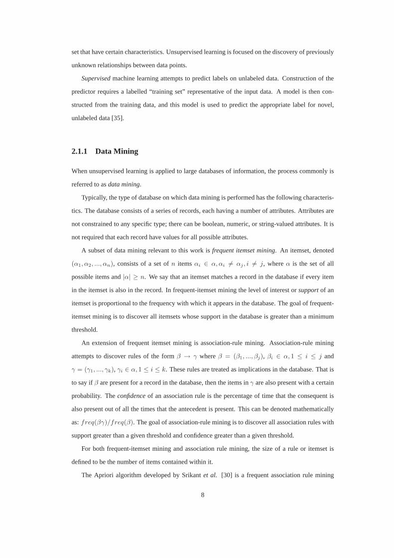
2.1 Example of path profiling information. . . . . . . . . . . . . . . .. . . . . . . . . 122.2 Example of edge profiling information. . . . . . . . . . . . . . . .. . . . . . . . . 122.3 Possible path profiling constructed from edge profiling information. . . . . . . . . 122.4 Upper path-profiling bounds based on edge profiling information. . . . . . . . . . 13
5.1 Total running time for FlowGSP, in seconds. . . . . . . . . . . .. . . . . . . . . . 505.2 Running times for FlowGSP by generation, in seconds, forN threads. . . . . . . . 505.3 Breakdown of execution time with 8 worker threads. . . . . .. . . . . . . . . . . 515.4 Influence of changing gap and window sizes on overall program performance. . . . 535.5 Execution time for the distributed implementation of FlowGSP withN workers. . . 55

List of Figures
2.1 Example of a portion of a program CFG. . . . . . . . . . . . . . . . . .. . . . . . 11
3.1 An example of a vertex-weighted, attributed flow graph. Edge weights are givenalong each edge and vertex weights are given next to each vertex. The letters in boldnext to a vertex are attributes of that vertex. . . . . . . . . . . . .. . . . . . . . . 23
3.2 The same graph as in figure 3.1 after edge weight and vertexcost normalization . . 233.3 Pathsp1 = {v1, v3, v7} andp2 = {v2, v4, v6} containing instances of the sequence
〈(A), (B), (E)〉 . . . . . . . . . . . . . . . . . . . . . . . . . . . . . . . . . . . . 283.4 Pathsp3 = {v6, v8} andp4 = {v7, v8} containing instances of the candidate se-
quence〈(E), (C)〉. . . . . . . . . . . . . . . . . . . . . . . . . . . . . . . . . . . 293.5 Small example of an Execution Flow Graph (EFG) . . . . . . . . .. . . . . . . . 35
4.1 Example of CFG annotated with edge profiling information. . . . . . . . . . . . . 44
5.1 Total speedup as a function of the number of threadsN . . . . . . . . . . . . . . . . 515.2 Speedup for the first through seventh generations as a function of the number of
threadsN . . . . . . . . . . . . . . . . . . . . . . . . . . . . . . . . . . . . . . . . 52
7.1 Example of a directed graph and a weighted traversal. . . .. . . . . . . . . . . . . 64

List Of Acronyms
AGI Address–Generation Interlock . . . . . . . . . . . . . . . . . . . . . . . .. . . . . . . . . . . . . . . . . . . . . . . . . . . . . 15
AOT Ahead-Of-Time . . . . . . . . . . . . . . . . . . . . . . . . . . . . . . . . . . . . . .. . . . . . . . . . . . . . . . . . . . . . . . . . . . 13
API Abstract Programming Interface . . . . . . . . . . . . . . . . . . . . . . .. . . . . . . . . . . . . . . . . . . . . . . . . . . . 18
BTB Branch Transition Buffer . . . . . . . . . . . . . . . . . . . . . . . . . . . . .. . . . . . . . . . . . . . . . . . . . . . . . . . . . 65
CFG Control Flow Graph . . . . . . . . . . . . . . . . . . . . . . . . . . . . . . . . . . .. . . . . . . . . . . . . . . . . . . . . . . . . . . 10
CPMF Central Processor Measurement Facility . . . . . . . . . . . . . . . .. . . . . . . . . . . . . . . . . . . . . . . . . . . 16
EFG Execution Flow Graph. . . . . . . . . . . . . . . . . . . . . . . . . . . . . . . . .. . . . . . . . . . . . . . . . . . . . . . . . . . .22
FDO Feedback–Directed Optimization . . . . . . . . . . . . . . . . . . . . . .. . . . . . . . . . . . . . . . . . . . . . . . . . . . 10
JDBC Java Database Connectivity . . . . . . . . . . . . . . . . . . . . . . . . . . .. . . . . . . . . . . . . . . . . . . . . . . . . . . . 40
JEE Java Enterprise Edition . . . . . . . . . . . . . . . . . . . . . . . . . . . . . .. . . . . . . . . . . . . . . . . . . . . . . . . . . . . 16
JVM Java Virtual Machine . . . . . . . . . . . . . . . . . . . . . . . . . . . . . . . . .. . . . . . . . . . . . . . . . . . . . . . . . . . . . 53
GSP Generalized Sequential Pattern . . . . . . . . . . . . . . . . . . . . . . .. . . . . . . . . . . . . . . . . . . . . . . . . . . . . . 9
ISA Instruction Set Architecture . . . . . . . . . . . . . . . . . . . . . . . . .. . . . . . . . . . . . . . . . . . . . . . . . . . . . . . 15
JIT Just-In-Time. . . . . . . . . . . . . . . . . . . . . . . . . . . . . . . . . . . . . . .. . . . . . . . . . . . . . . . . . . . . . . . . . . . . .10
MPI Message Passing Interface . . . . . . . . . . . . . . . . . . . . . . . . . . . .. . . . . . . . . . . . . . . . . . . . . . . . . . . . 18
PDF Profile–Directed Feedback . . . . . . . . . . . . . . . . . . . . . . . . . . . .. . . . . . . . . . . . . . . . . . . . . . . . . . . . 13
SVM Support Vector Machine . . . . . . . . . . . . . . . . . . . . . . . . . . . . . . .. . . . . . . . . . . . . . . . . . . . . . . . . . . 62
SPEC Standard Performance Evaluation Corporation . . . . . . . . . . .. . . . . . . . . . . . . . . . . . . . . . . . . . . 62
TLB Translation Lookaside Buffer . . . . . . . . . . . . . . . . . . . . . . . . .. . . . . . . . . . . . . . . . . . . . . . . . . . . . 14
1

2
Chapter 1
Introduction
Modern optimizing compilers are powerful tools in the pursuit of improved program performance.
Ultimately the ability of optimizing compilers to achieve good program performance is reliant on
the quality of the optimizations performed. These optimizations are the result of many person-hours
of hand tuning and investigation [6].
The development of these optimizations is a long process heavily dependant on the intuition and
skill of the compiler developer. Typically the investigation of new optimization opportunities starts
with the examination of current program performance. Once an opportunity has been identified,
the developer can then design and test an optimization. The entire process from investigation to
implementation can be extremely lengthy.
Typically, performance defects that merit the attention ofa compiler designer come in two dis-
tinct forms. The first consists of events that occur infrequently but incur a large cost. The second
type of defect is that which incurs a modest cost, but occurs very frequently. Identification of the
first type of defect is important to program performance and it is relatively simple to address. The
second type of performance issue is also important althoughmuch more difficult to discover.
Hardware performance counters are a common method for evaluating the performance of ap-
plications. Low-level information such as instruction cache misses, Translation Lookaside Buffer
(TLB) misses, and data cache misses can illuminate many aspects of program behavior that may be
potential targets for new optimizations. However, raw hardware profiles can be extremely verbose
making the identification of performance defects difficult.Many optimization opportunities may go
unnoticed simply due to the volume of information that must be examined. If performance defects
in hardware profiles could be identified more rapidly, then new optimizations could be developed at
3
a much faster pace.
Large enterprise applications, in particular, are an excellent example of how difficult it may be
to extract meaningful performance information from hardware performance profiles. For example,
the IBM R© WebSphereR© Application Server is a Java Enterprise Edition (JEE) enterprise server
written in JavaTM. A typical Application Server profile consists of thousandsof individual methods,
no one of which comes remotely close to dominating the total execution time. Such profiles are
often referred to as “flat” profiles as the histogram of execution time per region of code shows few
discernible peaks. Performance improvements are not likely to be achieved by considering individ-
ual methods; the entirety of the Application Server must be taken into account when designing code
transformations: a daunting task.
The field of data mining is devoted to the identification of patterns in data sets. An automated
analysis of the hardware profile data may be able to identify performance issues. In order to accom-
plish this, two goals must be accomplished:
1. A data structure must be designed to represent the data contained in the hardware profile. This
data structure must allow both the frequency and cost of defects to be identified.
2. An algorithm must be developed to search the data structure for patterns that correspond to
performance defects in the profiling data. This algorithm needs to rank patterns in accordance
with both their frequency and cost.
Generally, the hardware profiles of enterprise applications such as the WebSphereR© Application
Server are very flat. A profile is referred to as flat if no singlemethod accounts for a significant
proportion of the total execution time. In other words, the histogram of execution time spent on
each region of code shows no discernible peaks. This characteristic of enterprise application profiles
makes identification of worthwhile performance defects even more problematic.
The thesis presented in this document is:
A suitable data mining algorithm should be able able to discover patterns in a flat profile.
Some of these patterns should enable compiler designers to create new code transfor-
mations to improve the runtime performance of applications.
This thesis presents FlowGSP, a modification of the Generalized Sequential Pattern (GSP) algo-
rithm [32], and uses it to perform data mining on an ExecutionFlow Graph (EFG) constructed from
performance-counter data and Control Flow Graph (CFG) information extracted from the compiler.
4

The goal of this system is to aid in the identification of patterns in WebSphere-Application profiles
which may be indicative of new opportunities for code transformation.
The main contributions of this thesis are:
• The development of an EFG to model the information containedin hardware-profile data.
EFGs contain information that allows for the identificationof patterns based on their fre-
quency and on their relative weight.
• The development of FlowGSP, a data-mining algorithm designed to mine EFGs for patterns
corresponding to frequent and/or costly performance defects in hardware profiles.
• The development of two parallel implementations of FlowGSPin Java: one based on Java
threads for use on multi-core workstations and one based on sockets for use on distributed
systems. These implementations reduce the total executiontime of FlowGSP on WebSphere
Application Server profiles to the point where it is practical to use FlowGSP in a compiler
development environment.
• A report of the use of FlowGSP to identify performance defects in hardware profiles of the
WebSphere Application Server running on the IBM System z10TMarchitecture.
Chapter 2 provides background information on the technologies on which FlowGSP is based.
Chapter 3 details the FlowGSP algorithm and Chapter 4 outlines its implementation. A parallel im-
plementation and its performance is given in Chapter 5. Chapter 6 lists patterns discovered through
the use of FlowGSP and the performance opportunities exploited by their discovery. Works related
to this thesis are discussed in Chapter 7.
5

6

Chapter 2
Background Information
Mining interesting sequences from hardware profiles requires knowledge from multiple disciplines
in computing science. Knowledge of machine learning (specifically unsupervised learning and data
mining), compiler architecture, parallel algorithm construction, and low-level system architecture is
required in order to properly address the mining problem. This section briefly outlines background
information that may be needed to understand FlowGSP, its implementation, and its application to
mining hardware profiles.
Section 2.1 provides a high-level overview of machine learning techniques, with emphasis on
data mining. Section 2.2 discusses the difference between edge profiling and path profiling. Hard-
ware performance counters are discussed in Section 2.3, andSection 2.4 discusses specifics of the
IBM System z10 architecture on which the profiles were collected. The WebSphere Application
Server, which is the application studied in this work, is discussed in Section 2.5. Section 2.6 dis-
cusses measuring the performance of parallel algorithms.
2.1 Machine Learning
Machine learning, or statistical learning, can be defined asthe use of statistical techniques to auto-
matically extract meaningful information from data. Machine learning is divided into two categories:
supervised learning and unsupervised learning. The goals and methodology of these two types of
machine learning can greatly differ and as such it is important to differentiate between them.
Unsupervisedmachine learning techniques attempt to automatically assign labels to an unlabeled
data set, for example by finding patterns or identifying clusters of similar items [35]. Unsupervised
learning algorithms are not search algorithms. Search problems look for an entry or entries in a data
7
set that have certain characteristics. Unsupervised learning is focused on the discovery of previously
unknown relationships between data points.
Supervisedmachine learning attempts to predict labels on unlabeled data. Construction of the
predictor requires a labelled “training set” representative of the input data. A model is then con-
structed from the training data, and this model is used to predict the appropriate label for novel,
unlabeled data [35].
2.1.1 Data Mining
When unsupervised learning is applied to large databases of information, the process commonly is
referred to asdata mining.
Typically, the type of database on which data mining is performed has the following characteris-
tics. The database consists of a series of records, each having a number of attributes. Attributes are
not constrained to any specific type; there can be boolean, numeric, or string-valued attributes. It is
not required that each record have values for all possible attributes.
A subset of data mining relevant to this work isfrequent itemset mining. An itemset, denoted
(α1, α2, ..., αn), consists of a set ofn itemsαi ∈ α, αi 6= αj , i 6= j, whereα is the set of all
possible items and|α| ≥ n. We say that an itemset matches a record in the database if every item
in the itemset is also in the record. In frequent-itemset mining the level of interest orsupportof an
itemset is proportional to the frequency with which it appears in the database. The goal of frequent-
itemset mining is to discover all itemsets whose support in the database is greater than a minimum
threshold.
An extension of frequent itemset mining is association-rule mining. Association-rule mining
attempts to discover rules of the formβ → γ whereβ = (β1, ..., βj), βi ∈ α, 1 ≤ i ≤ j and
γ = (γ1, ..., γk), γi ∈ α, 1 ≤ i ≤ k. These rules are treated as implications in the database. That is
to say ifβ are present for a record in the database, then the items inγ are also present with a certain
probability. Theconfidenceof an association rule is the percentage of time that the consequent is
also present out of all the times that the antecedent is present. This can be denoted mathematically
as:freq(βγ)/freq(β). The goal of association-rule mining is to discover all association rules with
support greater than a given threshold and confidence greater than a given threshold.
For both frequent-itemset mining and association rule mining, the size of a rule or itemset is
defined to be the number of items contained within it.
The Apriori algorithm developed by Srikantet al. [30] is a frequent association rule mining
8

algorithm. The Apriori algorithm is so named because it is based on what the authors call the apriori
principle: in order for a pattern to be frequent, all of its sub-patterns must be frequent as well [30].1
Apriori searches for all rules up to a given size with a minimum support and confidence.
Apriori is an iterative generate-and-test algorithm. The first iteration is given an initial set of
candidate itemsets consisting of all possible sequences ofsize 1. The database is scanned, and the
support and confidence of each itemset is calculated. Any candidates that do not meet the minimum
support and confidence thresholds are removed. The candidate itemsets for the next iteration are
generated by joining the surviving items of the previous generation of candidates. This process
continues until either a set number of iterations has been completed or no candidates survive the
pruning process.
2.1.2 Frequent-Sequence Mining
An extension of frequent itemset mining isfrequent sequence data mining, or frequent sequence
mining. Sequences in frequent sequence mining, denoted〈I1, I2, ..., In〉, consist of a series of item-
setsI as previously defined. Databases mined for frequent sequences usually contain a number of
data sequences, each of which is a totally ordered sequence of records. Any itemsetI discoverable
through frequent itemset mining corresponds to the sequence 〈I〉 which can be discovered through
frequent-sequence mining. Thus frequent-itemset mining is a subset of frequent-sequence mining.
A sequence〈I1, I2, ..., , In〉matches a series of recordsR1, R2, ..., Rn if and only if:
• ∀α ∈ Ii, α ∈ Ri, 1 ≤ i ≤ n.
• For eachRi, i < n, Ri immediately precedesRi+1.
Many algorithms allow for an additional parameterg which specifies the maximum distance between
Ri, Ri+1 in a sequence.
The support of a sequence is typically defined to be the numberof data sequences in which
the sequence appears. Most frequent sequence mining algorithms do not count support for multiple
instances of a sequence in the same data sequences. Confidence is not included as a metric of support
unless the algorithm is also mining for association rules.
2.1.3 GSP
Our algorithm is based on a frequent-sequence algorithm called the Generalized Sequential Pattern
(GSP) algorithm [32]. GSP is an iterative generate-and-test algorithm.1Note that this has no connection witha priori or a posteriorireasoning.
9

GSP does allow for flexibility in how to determine if a sequence matches a series of records
by introducing two additional parameters: maximum gap sizeand maximum window size. The
maximum gap size determines how many vertices may occur betweenRi andRi+1. The maximum
window size determines how many records to consider in unison when matching each itemset in
a sequence. Formally, a window size ofw means that a itemsetI will match a series of records
Ri, Ri+1, ..., Ri+w if ∀α ∈ I, α ∈ Ri ∪Ri+1 ∪ ... ∪Ri+w.
2.2 Compiler Technology
Hardware profiles are not the only source of information regarding characteristics of a given pro-
gram. Compilers contain detailed representations of the program being compiled. This information
is used to perform a myriad of code transformations aimed at improving program performance. Un-
derstanding both the design process for new code transformations and the internal data structures of
the compiler is important if we are to search for patterns that are of use to compiler developers.
Compilers can be divided into two distinct categories: static compilers and Just-In-Time (JIT), or
dynamic, compilers. Static compilers are the most common, converting source into native executable
code prior to program execution. JIT compilers run in tandemwith an interpreter or virtual machine,
dynamically compiling sections of the interpreted programto native code during runtime.
The most relevant aspects of compiler technology for this thesis are the representation of pro-
gram flow, the collection of information about the relative frequency of execution of different por-
tions of the program through profiling, and the use of this information, in a process called Feedback–
Directed Optimization (FDO), to improve the performance ofa program. The remainder of this
section discusses these aspects.
2.2.1 Control Flow Graphs (CFGs)
Graphs are ubiquitously used as a way to represent the flow of execution in a program. Nearly all
optimizing compilers use a graph called CFG to represent theprogram being compiled. As the name
suggests, a CFG represents possible flow of control in the program.
Formally, a CFG is a graphG = {V,E, Fe} defined as follows:
• V is a set of vertices.
• E is a set of directed edges(vx, vy) wherevx, vy ∈ V .
• Fe is a function mapping edges inE to integer values.
10

Vertices inV represent units of execution in the program, usually basic blocks. Edges indicate
program flow between vertices. The functionFe maps each edgee ∈ E to an integer value indicating
the frequency of execution ofe. A CFG is a flow graph. Therefore the sum of the frequenciesFe
on the edges leading into any given vertex must be equal to thesum of the frequencies on the edges
leading out of the vertex.
The scope of a CFG is the same as the compilation unit of the compiler that created it. static
compilers typically analyze a single source file at a time. Asa result, the CFGs constructed by static
compilers consist of multiple single-entry single-exit regions corresponding to different procedures
in the source file. JIT compilers typically analyze individual methods in isolation, constructing a
single CFG for each method.
2.2.2 Edge Profiling vs. Path Profiling
It is important to distinguish edge profiling from path profiling. Edge profiling records only the num-
ber of times that each edge is the CFG was traversed during execution. Path profiling records how
many times an entirepath was executed. The difference between the two forms is best illustrated
with an example.
A
B C
D
E F
G
Figure 2.1: Example of a portion of a program CFG.
Consider the graph presented in Figure 2.1 to be an excerpt from a program CFG. Consider as an
example that the region of code represented by the CFG in Figure 2.1 is executed five times, taking
the following paths on each execution:
1. A→ B → D → F → G
2. A→ C → D → E → G
3. A→ C → D → F → G
4. A→ B → D → F → G
5. A→ C → D → E → G
11
Table 2.1 shows how the above information would be encoded asa path profile. Contrast this
profile with table 2.2 which shows the same information encoded as an edge profile.
Path Freq.A→ B → D → F → G 2A→ C → D → E → G 2A→ C → D → F → G 1
Table 2.1: Example of path profiling information.
Edge Freq.A→ B 2A→ C 3B → D 2C → D 3D → E 2D → F 3E → G 2F → G 3
Table 2.2: Example of edge profiling information.
The edge profiling information shown in Table 2.2 can be computed from the path profiling of
Table 2.1. However, the path profiling information cannot bederived from the edge profiling. For
instance, the path profiling shown in Table 2.3 could result from the same edge profiling information
in Table 2.2.
Path Freq.A→ B → D → E → G 2A→ C → D → F → G 3
Table 2.3: Possible path profiling constructed from edge profiling information.
FlowGSP mines edge profile data for sequences of attributes.Thus FlowGSP mines an upper
bound for the possible execution of the sequences in the program. For example, the upper bound on
path frequencies for the edge profiling of Table 2.2 is given in Table 2.4.
Path profiling is a much more precise representation of program execution. Path profiling is
often referred to astracing. However, for large programs, or long periods of execution,path profiling
becomes increasingly impractical due to the amount of storage space required. Edge profiling, while
less exact, is much more practical in these circumstances.
2.2.3 Dynamic Optimization
The heuristics that guide most standard compiler code transformations are based onstatic program
information, that is to say information that can be obtained by analyzingthe program source code
or CFG. Unfortunately, static information is insufficient to fully predict a program’s behavior at run
12

Path Freq.A→ B → D → E → G 2A→ B → D → F → G 2A→ C → D → E → G 2A→ C → D → F → G 3
Table 2.4: Upper path-profiling bounds based on edge profiling information.
time. For this reason it is difficult, if not impossible, to achieve optimal program performance using
code transformations that are based on static information alone. In order to more accurately model
program behavior, statistics obtained during program execution can be used in addition to static in-
formation. Such additional information is calleddynamic information. When code transformations
use this information the process is calleddynamic optimization.2
In addition, dynamic optimization also allows the collection of edge-frequency information to
add to the CFG of the program being compiled. This collectionis a form of edge profiling.
The rest of this section outlines the most common ways that modern optimizing compilers collect
runtime data.
Feedback-Directed Optimization
FDO, sometimes referred to as Profile–Directed Feedback (PDF), refers to the process where col-
lected runtime information from the previous execution of aprogram is used to make optimization
decisions about subsequent executions. The dynamic information required to make these optimiza-
tions is usually obtainedvia instrumentation hooks (in the case of Ahead-Of-Time (AOT) compilers)
or via online instrumentation (in the case of JIT compilers).
For AOT compilers, the data collected by the instrumentation hooks is written to disk after
execution has finished. This data is then fed back into the compiler via a command line parameter
on subsequent compilations and used to supplement the static program information. This process
is known asStatic Feedback Directed Optimizationas compilation occurs off-line,i.e. while the
program is not executing.
JIT compilation runtime data can be utilized while the program is still being executed. Programs
run under a JIT compiler can be recompiled multiple times during a single execution run with each
compilation ideally resulting in improved performance over the previous version. As such, programs
run under JIT compilers usually have to execute for a period of time before they reach a steady state.
This process is known asDynamic Feedback Directed Optimizationbecause compilation occurs
while the program is executing.
2Even though the compiler literature often talks about staticand dynamic “optimizations”, in most compiler developmentenvironments the designers implement heuristic-based code transformations. Often, the “optimal” case is not even defined.
13

Iterative Compilation
If the process of iterative search is applied to the optimization space of a program under an AOT
compiler, then the process is known as Iterative Compilation [18]. The idea behind iterative com-
pilation is that with each execution and recompilation performance is improved, even if slightly,
over the previous version. While iterative compilation doesresult in very fast code, it does so at the
cost of many recompilations and executions of the target program. While this large cost does make
Iterative Compilation unfit for general purpose computing,the technique can still be used for spe-
cialized cases where performance is crucial and it is difficult or impossible to update the application
once it has been deployed. Embedded systems and library optimization are fields in which iterative
compilation can provide substantial benefits [18, 6].
JIT compilation does bear some similarities with iterativecompilation. However, iterative com-
pilation is separate from JIT compilation because iterative compilation is done offline. Domains
that make frequent use of iterative compilation, such as embedded systems, are unlikely to use JIT
compilers. In addition, JIT compilers include compilationtime in the program runtime. Iterative
compilation is therefore unattrative from the perspectiveof a JIT compiler.
2.3 Performance Counters
Performance counters, or hardware profiling, allow programperformance at the hardware level to
be recorded. Events such as instruction cache misses, pipeline stalls, and Translation Lookaside
Buffer (TLB) misses to name a few are recorded by specializedhardware and then made available
to the user. Typically this information is obtained by sampling the machine state periodically after
a certain number of CPU cycles. This sampling period varies and can often be adjusted to suit the
application being profiled.
Typically performance counter data is gathered after execution has finished, however it is also
possible to gather this information while execution is occurring through the use of specialized li-
braries [27]. Schneideret. al. develop a custom run-time library to collect hardware counter infor-
mation about instruction-cache misses. The work done by Schneideret al. in this area only involves
a small number of performance counters [27]. It is unclear whether the performance overhead of
such libraries would become unmanageable on architectureswith a large number of performance
counters. Determining this overhead, however, is outside the scope of this thesis.
Performance counters are platform-specific entities; the types of events that are recorded and the
14

manner in which this recording is done varies from architecture to architecture.
2.4 z10 Architecture
The z10 is an in-order super-scalar CISC mainframe architecture from IBM [37]. “In-order” refers
to the fact that no hardware reordering of instructions occurs during execution. The z10 is an it-
erative advancement over the existing z9TMarchitecture [29], which is in turn an evolution of the
s390TM [26].
In modern architectures it takes multiple CPU cycles to decode, prepare, and execute even a
single assembly instruction. The z10 is a pipelined machinewhere, at any given moment, mul-
tiple instructions are at different stages of decoding or execution in order to increase instruction
throughput. Each core in the z10 has its own associated pipeline. The z10 pipeline is optimized
so that register-register, register-storage, and storage-storage instructions share the same pipeline
latency [37].
2.4.1 Address Generation Interlock
The z10 employs an Address–Generation Interlock (AGI) pipeline. AGI pipelines are designed to
avoid hazards introduced by load-use dependencies in the instruction pipeline [12]. However, this
form of pipeline design introduces another type of hazard. AGI stalls occur when a memory address
that is required by an instruction has not yet been computed when the instruction reaches a certain
stage in the pipeline. The missing address causes executionto stall until the address generation
completes. The hardware cannot let other instructions proceed ahead of the blocked instruction
because the z10 is an in-order machine.
There are two common ways to avoid AGI stalls. The first is to ensure that an address calculation
and corresponding use are spread far enough apart. The second is to select instructions from the
System z10 Instruction Set Architecture (ISA) that are designed to minimize AGI penalties [37]. In
either case, the onus falls on the compiler to produce code that avoids AGI stalls. Failure to do so
can result in a significant decrease in program performance.
2.4.2 Page Sizes
Most computer architectures transfer data between long-term storage, such as hard disks and main
memory, in fixed-length contiguous blocks called pages. A page normally contains 4 KB of data.
15

IBM System z10 allows for large pages that contain 1 MB of data[36]. Large pages are turned off
or onvia a command-line parameter given to the compiler.
2.4.3 Performance Counters on z10
The z10 Central Processor Measurement Facility (CPMF) includes numerous hardware performance
counters. There are two types of counters: sampled countersand event-based counters [17]. Sam-
pled counters are, as the name suggests, periodically sampled. Every set number of clock cycles
the architecture is queried, and it’s state recorded. If events of interest are in the process of oc-
curring, then the corresponding counters are incremented.Event-based counters are automatically
incremented each time the event occurs. Sampled counters record a measure of how much time was
spent handling various events, and event-based counters measure how often these events occurred.
Instructions on the z-series are typically grouped in pairs. This often results in performance-
counter information for one of the instructions being associated with the other and vice versa. While
this clustering of instructions does introduce imprecision into the data, this imprecision is extremely
localized and when taken over a large enough profile should not significantly affect overall trends in
the data.
2.5 WebSphere Application Server
The WebSphere Application Server is a full-featured Java Enterprise Edition (JEE) server developed
by IBM and written in Java [1]. A key characteristic of the WebSphere Application Server that makes
it interesting for study is that execution time is spread relatively evenly over hundreds of methods.
This even and thin distribution of execution time is a typical characteristic of enterprise applications
and other middleware. In addition, there are generally veryfew loops that are executed during the
processing of a query. Nagpurkaret al. stated that while each method occupies no more than 2% of
total execution time instruction-cache misses make up 12% of total execution time [22]. In addition,
if we want to capture 75% of all instruction-cache misses we must aggregate roughly 750 methods.
Therefore, optimizing any one method is not likely to make a significant impact on overall program
performance. Characteristics such as this require programbehavior to be examined beyond the scope
of a single method in order to accomplish efficient optimization of WebSphere Application Server.
At the same time it is impractical to thoroughly optimize theentirety of WebSphere Application
Server due to its size and number of methods. Thus, decisionsmade about how and what to optimize
must yield as much global benefit as possible whilst keeping compilation overhead to a minimum.
16
2.5.1 Profiling WAS
WebSphere Application Server is typically run using the IBMTestarossaR© JIT compiler. For this
reason, and the reasons discussed in Section 2.2.3, it is important that when attempting to profile
the Application Server that the proper amount of burn-in time be allowed to pass to ensure that the
majority of the code being executed has been compiled to native code. For the purposes of this work,
whenever profiling data is being discussed it is assumed thatthis data has been collected after the
burn-in period and consists almost entirely of code produced by the JIT compiler. Specific details
about data collection are addressed in Chapter 4.
2.6 Parallel Performance
The typical metric for program performance is raw executiontime. However, this measure of per-
formance is insufficient for programs which execute in parallel. Speed is still ultimately the goal;
however the number of parallel components being executed needs to be considered as well.
The metric by which the performance of parallel programs is measured is how quickly program
execution time decreases as the amount of parallelism is increased. This is referred to asspeedup,
a number representing the program’s execution time relative to the sequential case. Speedups is
calculated as follows:
s =tparallel
tsequential
wheretsequential is the execution time of the sequential version of the algorithm andtparallel is the
execution time of the parallel version of the same algorithm. A value ofs > 1 indicates a perfor-
mance improvement over the sequential case, whereas a valueof s < 1 indicates worse performance.
2.6.1 Linear Speedup
Ideally, if a task is split inton equal subsections we would expect the work to take1n
of the amount of
time, i.e. achieve a speedup ofn. This is referred to aslinear speedup, as the curvespeedup = f(n)
is exactly equal to the linef(x) = x.
However, linear speedup is not always obtained in practice because some problems cannot be
completely decomposed into parallel portions. Say that therunning time of an algorithm takes time
t = p + q, wherep is the amount of time taken to execute the potentially parallel portion(s) of the
algorithm andq is the amount of time taken to execute the portion(s) of the algorithm that cannot
be parallelized. The maximum amount of possible speedup istq, as even if we have infinite parallel
17

resources to makep insignificant the algorithm will still take timeq to execute.
When considering sublinear, linear, or superlinear speedups, it is important to consider the fac-
tors that limit performance. In the early days of parallel programming most applications were bound
by the capacity of the processor to execute instructions. Therefore, adding a second processor was
expected to reduce the execution time at most by half. That is, a linear speedup was the best that
one could hope for. Sub-linear speedups were explained by poor load-balancing, communication
and sequencing overhead, contention for common resources,etc. Super-linear speedups typically
indicated an error in the measurement of performance.
However, in contemporary computers, the capacity of the processor to execute instructions is no
longer the limiting factor for performance. In many applications the processor is idle for most of the
time. The memory hierarchy and contentions in the network are more likely to limit performance.
The relationship between the number of processing nodes andperformance is no longer linear. In
these architectures, non-linear relations, both sub- and super-linear, between performance and the
number of processing nodes should be expected.3
2.6.2 Memory Organization
An important factor to consider when discussing parallel systems is the type of memory organization
in use. Typically organization falls into three categories: shared memory, distributed memory, and
distributed-shared memory.
In shared memory, each worker has access to a single, shared pool of memory. Communication
between workers is usually implicit; one worker will write to an area of memory and another worker
will read the same area. Shared memory is typical of threadedsystems such aspthreads or Java
threads.
In distributed memory systems, such as clusters, each worker executes within its own address
space and communication between workers must occur explicitly. This communication is usually
performed through some external Abstract Programming Interface (API) such as UNIX or Windows
sockets or Message Passing Interface (MPI). Distributed memory systems are commonly found in
single-processor clusters.
Distributed-shared memory is a hybrid organization where groups of processors communicate
via messages with processors in other groups. Each group of processors has access to a common
3An example of a super-linear speedup would be a case where a problem does not fit entirely into cache when operatingon a single CPU. Adding a second CPU doubles the amount of available cache so that the problem now fits entirely insidethe combined CPU caches. Alba investigates superlinear speedups in the domain of Parallel Evolutionary Algorithms; manyof his conclusions are also relevant to general parallel computing[3].
18

area of shared memory. Distributed-shared memory is typical of clusters with multi-core nodes.
19

20
Chapter 3
FlowGSP
The theoretical basis for an algorithm is as important as itspotential application. FlowGSP is based
on GSP [32], which is a well-established algorithm for mining frequent sequences in a database.
However, a sequence of records is a poor choice to represent program control flow. Therefore, in
order to effectively mine program data a new data structure must be defined to accurately represent
program behavior. Graphs are commonly used to represent thestructure of a program in most
compilers, and therefore it makes sense to develop a graph-based data structure on which mining
can be performed. Such a data structure is introduced in Section 3.1.
Once this new data model has been defined it is then necessary to define how to measure the
support of frequent sequences in this data structure. The goal of FlowGSP is to discover frequent
and/or costly sequences of attributes in an execution flow graph. In the original GSP algorithm,
the support of a sequence was defined as the number of data sequences in which the candidate
sequence occurred [32]. Given the motivation behind the development of FlowGSP this definition is
insufficient. The traditional definition ignores sequencesthat occur multiple times in the same data
set. In the scope of the execution of a program a sequence thatoccurs multiple times in the same
method is of interest to compiler developers. In addition tothe frequency of a sequence, FlowGSP
is also interested in the cost of these sequences. For these reasons the definition of support for
a subpath must differ from the classical definition of support used by GSP. Section 3.2 defines
support over our new data structure.
21

3.1 Edge and Vertex Weighted Attributed Flow Graphs
While our work was focused on mining hardware profiling data, there are many other applications
where mining weighted and attributed flow graphs may be useful. This section formally describes
such a data structure as well as how support values are calculated for subpaths within it.
3.1.1 Formal Definition
Let G = {V,E,A, F,W} be an Execution Flow Graph (EFG) such that:
• V is a set of vertices.
• E is a set of edges(va, vb), whereva, vb ∈ V .
• A(v) 7→ {α1, ..., αk} is a function mapping verticesv ∈ V to a subset of attributes
{α1, ..., αk}, αi ∈ α, 1 ≤ i ≤ k whereα is the set of all possible attributes
• F (e) 7→ [0, 1] is a function assigning a normalized frequency to each edgee ∈ E. i.e.∑
e∈E
F (e) = 1.
• W (v) 7→ [0, 1] is a function assigning a normalized weight to each vertexv ∈ V . i.e.∑
v∈V
W (v) = 1.
The constraint below holds because G is a flow graph.
∑
(x,v0)∈E
F ((x, v0)) =∑
(v0,y)∈E
F ((v0, y))
F and W are completely independent quantities. In fact, it is this independence on which
FlowGSP is based. Rather than define the importance of a sequence merely by its frequency
FlowGSP also considers the weight of the sequence in question.
Example
Figure 3.1 gives an example of a vertex-weighted attributedflow graph withα = {A,B,C,D,E}.
The same graph with edge weights and vertex costs normalizedis given in Figure 3.2. It is the graph
in Figure 3.2 that will be used as input to the mining algorithm.
22

A,D
15 5
5
515
6 9
6 9
10
4
18
10
1 7
9
13
A B
A,B,C
E
A,E D,E
C
20
v1
v2 v3
v4 v5
v6 v7
v8
Figure 3.1: An example of a vertex-weighted, attributed flowgraph. Edge weights are given alongeach edge and vertex weights are given next to each vertex. The letters in bold next to a vertex areattributes of that vertex.
A,D0.16 0.05
0.05
0.050.16
0.06 0.10
0.06 0.10
0.14
A B
A,B,C
E
A,E D,E
C
0.14
0.18
0.01
0.13
0.10
0.06
0.25
0.21
v1
v2 v3
v4 v5
v6 v7
v8
Figure 3.2: The same graph as in figure 3.1 after edge weight and vertex cost normalization
23

3.2 Calculating Path Support
A sequence of attributes in an EFG has a direct correspondence with a subpath in the same graph.
Support metrics are defined in terms of subpaths in the graph because subpaths are more specific
than sequences. This definition is then generalized to sequences of attributes.
In our program representation, sequences correspond to frequent or costly subpaths in the graph.
A subpathpk ∈ G of lengthl is an ordered set ofl vertices. The notationpk[i] refers to theith vertex
of pk. By definition in order forpk to be a subpath,(pk[i], pk[i + 1]) ∈ E for all 0 ≤ i ≤ g − 2.
The notationpk[i : j] refers to the subpath ofpk which consists of theith to jth vertices inclusive,
i ≤ j.
The support of a path, both in terms of its cost of execution and its frequency of execution, can
now be defined.
3.2.1 Frequency Support
In GSP, the support of a sequence was defined as the number of data sequences in which the se-
quence appeared. This definition was sufficient because the type of database being mined by GSP
typically consisted of a large number of short data sequences. However, multiple occurrences of a
sequence in an EFG should all contribute towards the supportfor a sequence. The rationale for this
decision is based on the motivating application of FlowGSP.A profile is an aggregation over multi-
ple executions of the same region of code. Therefore, to onlyallow a single instance of a sequence
per EFG could potentially discard many other executions of the same region. This is not dissimilar to
the methodologies employed in some algorithms that search for frequent subgraphs [16, 39, 14, 23].
In addition, the data sequences mined by GSP are all total orderings; they do not have the edge-
weighted topological structure present in EFGs. In GSP, each occurrence of a candidate sequence
is weighted equally. However it does not make sense to assignequivalent importance to two oc-
currences of a sequence in an EFG with different edge weightsas edge weights are a measure of
frequency. Therefore the edge weights must also be taken into account when determining the fre-
quency support of a candidate sequence. Based on the two reasons discussed here, the method for
calculating the frequency support for a candidate sequencemust be redefined.
The definition of the frequency support of a pathpk is based on the frequenciesF of the edges
that comprisepk. It can only be assumed thatpk was at most executed the same number of times as
the least-frequent edge in the path.
In order to account for the degenerate case where a path consists of only a single vertex and no
24

edges, the frequency supportSf of a single vertexv is defined as follows:
Sf (v) =∑
(va,v)∈E
F ((va, v))
In general, the frequency support of a pathpk is:
Sf (pk) = min{F (pk[0], pk[1]), . . . , F (pk[g − 2], pk[g − 1])}
3.2.2 Weight Support
In order to contrast the frequency and weight of a sequence inan EFG an additional metric of support
must be defined to represent the weight of a subpath in the EFG.The weight of a subpath is based
on the weights of its vertices. The weight support of a path iscalculated as follows:
Sw(pk) = min0≤j≤g−1
{W (pk[j])}
Similarly to the frequency support of a subpath, the maximumweight support of a subpath is
limited by the vertex in the path with the smallest weight.
3.3 Sequences of Attributes
Attributes are the method by which information about each vertex is encoded. Each vertex may
have as many attributes as is needed. The attributes assigned to each vertex will be the items in the
frequent sequences mined by FlowGSP.
Attributes in our representation are binary, taking a valueof either true or false. If a given
attributeαi is true for a vertexva thenva has the attributeαi. Conversely ifαi is false forva
thenva does not haveαi. By convention, attributes whose value is false are simply omitted. This
interpretation leads to an efficient representation in which only true attributes need to be recorded
for each vertex. This is especially important to reduce the storage space required to process large
EFGs.
Unfortunately, not all attributes associated with a vertexare binary values. Some attributes are
measures of some quantity associated with the vertex, and others may indicate which of a number
of classes the vertex may belong to.
Attributes that take a numerical value (integer or otherwise) are converted to a binary represen-
25

tation by comparison with a set threshold. Multiple thresholds may also be used in order to separate
the attribute’s values into ranges.
Enumerated attributes that can take one ofr possible values are represented byr mutually-
exclusive binary attributes, wherer is a known positive integer.
A sequenceS = 〈s0, s1, ..., sk−1〉 of lengthk is a sequence ofk sets of attributes, denoted by
si, 0 ≤ i < k. For convenience, thesubsequence〈si, ..., sj〉 of S is denoted asS[i, j], i ≤ j. If
i = j this subsequence is denoted asS[i].
3.3.1 Matching Sequences to Paths
Section 3.3 established how the frequency and weight support of a subpathpk in an EFGG are
calculated. All that remains in order to calculate the supports of a sequenceS is to formally establish
howS maps topk. Once this has been done, the supports are aggregated over all suchpk to determine
the supports ofS.
A subpath isminimalwith respect to a candidate sequenceS if both pk[0] andpk[g − 1] contain
part of the candidate sequence, that is to say the first and last vertices in the subpath are not skipped.
Henceforth all subpaths are assumed to be minimal with respect to the candidate sequence being
examined.
A subpathpk contains a sequenceS if ∀si ∈ S, si ⊆ A(pk[i]). This is a very rigid definition
where each set of attributessi ∈ S must occur on theith vertex ofpk. This definition can be
modified to allow for a more flexible matching. Indeed, this same manner of flexible matching was
implemented in GSP by Srikantet al. [31]; this flexibility has been extended to fit the context of an
EFG.
It is not required that the entirety of each set of attributesin a sequence be contained within
the attributes of a single vertex in the graph. One of the parameters of the mining algorithm is
the maximum windows size,wmax. Attributes that are observed on any vertices withinwmax are
considered to belong to the same set within a sequence. Maximum window size can be formally
expressed as follows:
si ∈⋃
v∈pk[l:l+w]
A(v), 0 ≤ w ≤ wmax
The shorthand notationsi ∈ A(pk[l : l + w]) will henceforth also refer to the above constraint.
Themaximum gap sizegmax is the maximum allowable distance between two verticesvx, vy ∈
pk where the following holds:
26
• vx is the last in a series of vertices that contains a set of attributess1.
• vy is the first in a series of vertices that contains a set of attributess2
• s1 ands2 are consecutive sets of attributes inS.
It is implicit in this definition that all of the vertices in the path betweenvx andvy do not contribute
any attributes toS.
Formally, we say that a subpathpk contains a sequenceS if and only if the following criteria
hold:
• ∀si ∈ S, si ∈ A(pk[l : l + w]) where0 ≤ w ≤ wmax
• ∀si, sj ∈ S, wheresi ∈ A(pk[l : l + w]) andsj ∈ A(pk[m : m + w′])
– pk[l : l + w] ∩ pk[m : m + w′] = ∅
– If j = i + 1 thenm = l + w + 1 + g whereg ≤ gmax
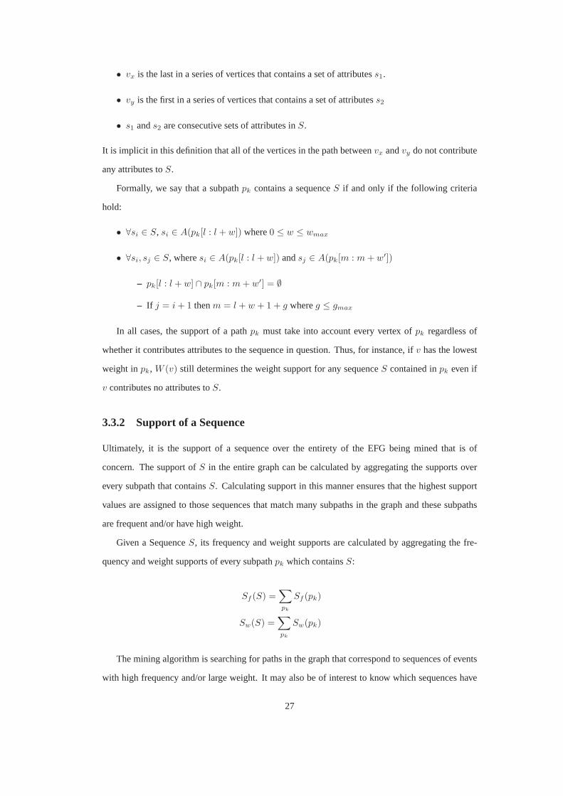
In all cases, the support of a pathpk must take into account every vertex ofpk regardless of
whether it contributes attributes to the sequence in question. Thus, for instance, ifv has the lowest
weight inpk, W (v) still determines the weight support for any sequenceS contained inpk even if
v contributes no attributes toS.
3.3.2 Support of a Sequence
Ultimately, it is the support of a sequence over the entiretyof the EFG being mined that is of
concern. The support ofS in the entire graph can be calculated by aggregating the supports over
every subpath that containsS. Calculating support in this manner ensures that the highest support
values are assigned to those sequences that match many subpaths in the graph and these subpaths
are frequent and/or have high weight.
Given a SequenceS, its frequency and weight supports are calculated by aggregating the fre-
quency and weight supports of every subpathpk which containsS:
Sf (S) =∑
pk
Sf (pk)
Sw(S) =∑
pk
Sw(pk)
The mining algorithm is searching for paths in the graph thatcorrespond to sequences of events
with high frequency and/or large weight. It may also be of interest to know which sequences have
27
disproportionate levels of frequency support compared to weight support or vice-versa. In order to
concisely capture the goals of the mining algorithm two additional measures of support are intro-
duced.
Themaximalsupport of a sequenceS is:
SM (S) = max{Sf (S), Sw(S)}
Thedifferentialsupport is:
SD(S) = |Sf (S)− Sw(S)|
The rationale behind these definitions is as follows. If one or both of Sf or Sw is high, then
it is likely that the sequence will be of interest either because it is frequent or because it is costly.
In addition, if there is a large difference betweenSf andSw then this means that the sequence in
question is either frequent but not costly, or costly but infrequent.
Example (continued)
A,D0.16 0.05
0.05
0.050.16
0.06 0.10
0.06 0.10
0.14
A B
A,B,C
E
A,E D,E
C
0.14
0.18
0.01
0.13
0.10
0.06
0.25
0.21
v1
v2 v3
v4 v5
v6 v7
v8
P1
P2
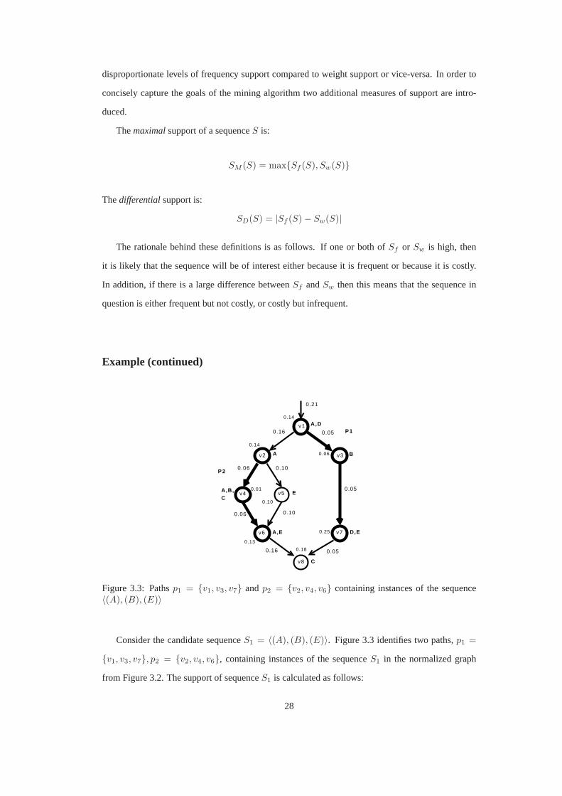
Figure 3.3: Pathsp1 = {v1, v3, v7} andp2 = {v2, v4, v6} containing instances of the sequence〈(A), (B), (E)〉
Consider the candidate sequenceS1 = 〈(A), (B), (E)〉. Figure 3.3 identifies two paths,p1 =
{v1, v3, v7}, p2 = {v2, v4, v6}, containing instances of the sequenceS1 in the normalized graph
from Figure 3.2. The support of sequenceS1 is calculated as follows:
28

Sf (p1) = min{0.21, 0.05, 0.05} = 0.05
Sf (p2) = min{0.16, 0.06, 0.06} = 0.06
Sf = 0.11
Sw(p1) = min{0.14, 0.06, 0.06} = 0.06
Sw(p2) = min{0.14, 0.01, 0.14} = 0.01
Sw = 0.07
Therefore, the total support for the sequenceS1 is:
SM = 0.11, SD = 0.04
A,D0.16 0.05
0.05
0.050.16
0.06 0.10
0.06 0.10
0.14
A B
A,B,C
E
A,E D,E
C
0.14
0.18
0.01
0.13
0.10
0.06
0.25
0.21
v1
v2 v3
v4 v5
v6 v7
v8P3 P4
Figure 3.4: Pathsp3 = {v6, v8} andp4 = {v7, v8} containing instances of the candidate sequence〈(E), (C)〉.
Now consider the candidate sequenceS2 = 〈(E), (C)〉. Figure 3.4 gives two paths,p3 =
{v6, v8}, p4 = {v7, v8}, containing instances ofS2. Note thatp3 andp4 share a common vertex in
this case. The supports for sequenceS2 are:
Sf (p1) = min{0.06 + 0.10, 0.16} = 0.16
Sf (p2) = min{0.05, 0.05} = 0.05
29

Sf = = 0.21
Sw(p1) = min{0.13, 0.18} = 0.13
Sw(p2) = min{0.25, 0.18} = 0.18
Sw = 0.31
Therefore, the total support for the sequenceS2 is:
SM = 0.31, SD = 0.10
3.4 FlowGSP
This section presents FlowGSP, an algorithm for mining sequences of attributes with either high
frequency or high cost. Pseudo-code for FlowGSP is presented in algorithm 1.
The parameters to FlowGSP are an EFG G, as defined in Section 3.1, the maximum gap size
gmax, the maximum window sizewmax, the number of generations to iteratengen, the threshold for
maximal supportSMthresh, and the threshold for differential supportSDthresh.
The graphG need not be the entire EFG that is being mined. The actual graph to be mined may
be subdivided into independent single-entry single-exit regions and FlowGSP may be applied to
each region individually. Support for each candidate is then aggregated over all regions. Currently,
inter-region sequences are not considered because a JIT compiler compiles individual methods in
isolation.
EFGs may contain cycles. In order to prevent traversing the graph infinitely around a cycle, a
list of previously visited vertices is maintained. Children that appear on this list are not added to
the queue of vertices. This restriction does not prevent thediscovery of sequences that occur across
loops in the graph; the list only ensures that FlowGSP startslooking for a matching path exactly
once at each vertex.
FlowGSP uses a hash treeH in order to reduce the number of candidate sequences that be
examined at each vertex. The creation of the hash treeH and the process of fetching candidate
sequences from it is derived from the process described in Srikant et.al. [32]. Candidates are added
to the hash tree by hashing on each attribute in the sequence,in order. The retrieval of candidates
from a node in the hash tree depends on the position of the nodein the tree:
• root node: Move to the next node in the tree by hashing on each attribute of v and any vertex
30

Algorithm 1 : FlowGSPFlowGSP(G, gmax, wmax, ngen, sMthresh, sDthresh)
1: G1 ← Create F irst Generation(α)2: n← 13: while Gn 6= ∅ ∧ n < ngen do4: H ← Create Hash Tree(Gn)5: v0 ← First vertex inG6: Q.push(v0)7: alreadySeen← ∅8: while Q 6= ∅ do9: v ← Q.pop()
10: alreadySeen← alreadySeen ∪ v11: C ← H.get candidates(v)12: for S ∈ C do13: supports← Find Paths(S, v, 0, true, gmax, wmax)14: for (Sw, Sf ) ∈ supports do15: Sw(S)← Sw(S) + Sw
16: Sf (S)← Sf (S) + min{Sf , Sf (v)}17: end for18: end for19: for v′ ∈ children(v) do20: if v′ /∈ alreadySeen then21: Q.push(v′)22: end if23: end for24: end while25: for S ∈ Gn do26: if SM (S) < sMthresh ∧ SD(S) < sDthresh then27: Gn ← Gn \ S28: end if29: end for30: if n < ngen − 1 then31: Gn+1 ←Make Next Gen(Gn)32: end if33: n← n + 134: end while
31

within wmax from v. Pass along the set of attributes that we have not yet hashed on.
• interior node: Move to the next node in the tree by hashing on each of the remaining attributes
passed in. If none remain, add the attributes of the next vertex/vertices to the set of attributes
and continue.
• leaf node: Return all candidates present on the leaf node.
Rather than hashing on the attributes of all data items with atime stamp in the given window,
FlowGSP hashes on the attributes of the current vertex and ofall its descendants that fit within the
specified window size. For instance, forwmax = 0, H.get candidates(v) in Line 11 of Algorithm 1
would return all sequences that start with an attribute associated with vertexv.
The rest of this section outlines the FlowGSP algorithm in more detail.
3.4.1 Creation of Initial Generation
Create F irst Generation takes the set of all possible attributes and returns a set of candidates,
where each candidate contains one of the possible attributes and there exists a candidate for every
attribute. Formally, this can be expressed as:
G1 = Create F irst Generation(α)
where the following two constraints hold:
G1 = {〈(αi)〉|αi ∈ α}
∀αi ∈ α, 〈(αi)〉 ∈ G1
For example, supposeα = {A,B,C,D,E}. The result of callingCreate F irst Generation(α)
would be:
G1 = {〈(A)〉, 〈(B)〉, 〈(C)〉, 〈(D)〉, 〈(E)〉}
Both the weight support and frequency support of each sequence are initialized to zero. For instance,
in this example:
Sf (〈(A)〉) = 0
Sw(〈(A)〉) = 0
32

3.4.2 Matching Path Discovery
To discover all subpaths that contain a candidate sequenceS FlowGSP employs the following strat-
egy. Each vertexv in the graph is considered as a potential starting point for asubpathpk that
contains a candidate sequenceS. The search for the subpath is conducted through a depth-first
search starting atv.
subpaths are found in a greedy fashion. That is, FlowGSP searches for the shortest subpath
pk that matches the given sequenceS starting at the current vertexv0. FlowGSP does not include
support from a subpathpn if there exists a subpathpm such that: pm ⊂ pn, pm and pn both
containS, andpm andpn share the same initial vertex. Consider again the example presented in
Section 3.3.1. The sequence〈(A), (D)〉 is contained in two minimal subpaths:pm = {va, vb}
andpn = {va, vb, vc} with vb not contributing any attributes. In this case FlowGSP wouldonly
return the subpathpm because it is the shortest. The rationale behind this decision is that any longer
subpath which also containsS has at most the same support as the shorter subpath.1 An argument
for including the supports ofpn while calculating supports forS is thatpn is capturing the event
where attributeA is observed, then attributeB is observed twice in succession. However this event
will be captured by the sequence〈(A), (B), (B)〉 that will be mined in a later iteration. Therefore,
given a starting vertexv, FlowGSP finds only the shortest path(s) that contains the current candidate
that start atv.
Algorithms 2 and 3 outlineFind Paths andFind Set, respectively, which conduct the depth-
first search for a subpath that matches a candidate sequence.Find Set searches for the next set
of attributes in the candidate sequence given the current window sizewmax. Find Paths then
searches for the starting point of the next set of attributesin the sequence within the given maximum
gap sizegmax. BothFind Paths andFind Set return a set of support tuples. Each tuple in this
set is formed by a weight supportSw and a frequency supportSf .
Find Paths andFind Set are mutually recursive. AfterFind Set finds a set of attributes,
it calls Find Paths to find the rest of the sequence.Find Paths in turn callsFind Set to find
the next set of attributes in the sequence. After the initialcall toFind Paths returns, the(Sw, Sf )
values are added to the frequency and weight support ofS. The recursion betweenFind Path and
Find Set is guaranteed to terminate. The search for a subpath that matches a sequenceS will stop
when either the sequence has been found, or when the maximum gap and maximum window size
has been exhausted and no matching subpath has been found. Therefore the search is guaranteed to
1This invariant holds because the frequency and weight supports are based on the edge with the lowest frequency or thevertex with the lowest weight respectively.
33
terminate in a finite amount of time becausewmax, gmax, and the size ofS are all constant.
Find Paths takes a parametergremain, indicating the remaining size of gap that may occur in
the current sequence. IfFind Set returns∅ andgremain = 0, thenFind Paths returns an empty
set. Similarly,Find Set has a parameterwremain that determines how many edges the algorithm
should traverse from the current vertex to find all the attributes that belong to the current set of
attributes. Ifwremain = 0, thenFind Set will return ∅ instead of investigating further vertices.
Find Paths also takes a boolean parameterfirstSet which is set to true if and only ifFind Paths
is searching for the start of the sequence. This parameter exists solely for the purpose of passing this
information toFind Set.
The initial call toFind Paths in algorithm 1 is given zero as the remaining gap regardless
of the value ofgmax, to ensure that the first set of attributes in the sequence starts on that vertex.
Therefore the subpath found is minimal.2
Find Set returns aSf value of infinity if there are no more itemsets left to find inS. This
value ofSf is assigned on Line 5 of Algorithm 3. Infinite support indicates thatFind Set has not
traversed any edges in order to find the current set of attributes. Therefore, there is no meaningful
value to return forSf . TheSf of the entire path is calculated by taking the minimum between the
new value and a previously computed value. Therefore, assigning a value of infinity ensures that
this new value will not alter the previously calculated value ofSf .
Find Set takes two parameters that together represent the set of attributes the algorithm is
searching for.sleft contains the attributes that we have yet to find, andsfound contains the attributes
that were previously located. On the initial call toFind Set from Find Path, sleft contains the
entire set of attributes andsfound = ∅.
Find Set also takes two boolean parameters,firstSet andstartOfFirstSet. firstSet is
set to true if and only ifFind Set is looking for the first set of attributes in the sequence, and
startOfFirstSet is true if and only ifFind Set is searching for the start of the first set of at-
tributes. The rationale behind these parameters is as follows.
firstSet is used on line 21 to ensure that we find the shortest sequence of vertices which matches
the current sequence. If the current vertex contains all of the attributes previously found on the first
set of a sequence then the subpath being explored is not minimal. ThereforefirstSet returns the
empty set. The shorter subpath will be discovered on a futurecall toFind Paths.
startOfFirstSet is required on line 18 to ensure that we do not allow a vertex which does not
2No steps need to be taken to ensure thatpk[g − 1] (i.e. the last vertex on the path) contributes to the sequence becausethe search for a matching path terminates at this point
34

contribute to the first item set to occur at the start of the subpath.
Algorithm 2 : Algorithm to find all paths that contain a sequenceS starting at a vertexv.
Find Paths(S, v, gremain, firstSet, gmax, wmax)
1: supports← Find Set(S[0], ∅, S, v, wmax, firstSet, firstSet, gmax, wmax)2: if supports 6= ∅ then3: returnsupports4: end if5: if gremain ≤ 0 then6: return∅7: end if8: for v′ ∈ children(v) do9: supports′ ← Find Paths(S, v′, gremain − 1, false, gmax, wmax)
10: for (Sw, Sf ) ∈ supports′ do11: Sw ← min{Sw,W (v)}12: Sf ← min{Sf , F ((v, v′))}13: supports← supports ∪ {(Sw, Sf )}14: end for15: returnsupports16: end for
Example
Figure 3.5 gives a small example of an EFG to illustrate the behavior ofFind Path andFind Set.
For this EFGα = {A,B}, gmax = 0, andwmax = 0.
0.25
0.375 0.125
0.25
AB
A
B
0.4
0.4
0.2
v1
v2
v3
Figure 3.5: Small example of an EFG
Consider thatFlowGSP has reached the vertexv2. Hashing on the attributes contained in
A(v2), the candidates that could potentially start onv2 in generationG2 are S1 = 〈(A), (A)〉,
S2 = 〈(A), (B)〉, andS3 = 〈(A,B)〉. FlowGSP then makes the following calls toFind Paths:
• Find Paths(S1, v2, 0, true, 0, 0). Find Paths immediately calls:
35

Algorithm 3 : Algorithm to find the next set of attributes in the sequence.
Find Set(sleft, sfound, S, v, wremain, firstSet, startOfFirstSet, gmax, wmax)
1: supports← ∅2: k ← |S|3: if sleft ⊆ A(v) then4: if k = 1 then5: supports = {(W (v),∞)}6: returnsupports7: end if8: for v′ ∈ children(v) do9: supports′ ← Find Paths(S[1, k − 1], v′, gmax, false, gmax, wmax)
10: for (Sw, Sf ) ∈ supports′ do11: Sw ← min{Sw,W (v)}12: Sf ← min{Sf , F ((v, v′))}13: supports = supports ∪ {(Sw, Sf )}14: end for15: end for16: returnsupports17: else18: if startOfFirstSet ∧A(v) ∩ sleft = ∅ then19: return∅20: end if21: if firstSet ∧ sfound ⊆ A(v) then22: return∅23: end if24: if wremain ≤ 0 then25: return∅26: end if27: Sleft ← sleft \A(v)28: Sfound ← sfound ∪ (A(v) ∩ sleft)29: for v′ ∈ children(v) do30: supports‘← Find Set(sleft, sfound, S, v′, wremain − 1, firstSet, false, gmax, wmax)31: for (Sw, Sf ) ∈ supports′ do32: Sw ← min{Sw,W (v)}33: Sf ← min{Sf , F ((v, v′))}34: supports← supports ∪ {(Sw, Sf )}35: end for36: end for37: returnsupports38: end if
36
– Find Set({A}, ∅, S1, v2, 0, true, true, 0, 0). S1[0] = A and thereforeS1[0] ⊆ A(v2).
Find Paths is called to search forS1[1] starting with the children ofv2.
∗ Find Paths(S1[1], v1, 0, false, 0, 0). Find Paths immediately calls:
· Find Set({A}, ∅, S1[1], v1, 0, false, false, 0, 0). S1[1] = A and therefore
S1[1] ⊆ A(v1). Find Set returns the tuple(0.4,∞) because|S1[1]| = 1 and
therefore we have found the entire sequence.
Find Set returned a non-empty set, thereforeFind Paths returns the same set.
Find Set setsSw = min{0.4, 0.4} = 0.4 and Sf = min{∞, 0.125} = 0.125.
(0.4, 0.125) is added to the set of support tuples.
Find Set now callsFind Paths to search the next child ofv2.
∗ Find Paths(S1[1], v3, 0, false, 0, 0). Find Paths immediately calls:
· Find Set({A}, ∅, S1[1], v3, 0, false, false, 0, 0). A(v3) = B, and therefore
S1[1] 6⊆ A(v3). Find Set. Find Set returns∅ becausewremain = 0.
Find Paths also returns∅ becauseFind Set returned∅ andgremain = 0.
Find Set returns the supports accumulated thus far because all of thechildren ofv2
have been explored.
Find Paths returns the set of supports returned byFind Set. These supports are added to
the support values ofS1.
FlowGSP then repeats the above procedure, callingFind Paths for S2 andS3.
In this example, the role ofFind Paths is diminished becausegmax = 0. If gmax > 0 then
Find Paths would explore children of the current vertex in the event that Find Set returns∅. This
exploration continues until the maximum gap size has been reached.
3.4.3 Candidate Generation
The creation of new candidates prior to the start of the next iteration byMake Next Gen is handled
exactly as in Srikantet al. [32]. A brief description is included here.
New candidates are created by joining compatible candidates in the current generation. Candi-
dates are defined as compatible if thesuffixof the first candidate is equal to theprefixof the second.
The suffix of a sequence is created by removing the firstattribute from the sequence. Note that
this is very different from removing the first set of attributes from the sequence. For example, the
suffix of the sequence〈(A,B), (C)〉 is 〈(B)(C)〉. The prefix of a sequence is likewise formed by
37

removing the last attribute of the sequence. The prefix of〈(A,B), (C)〉 is 〈(A,B)〉. A prefix and
suffix are defined to be equal if and only if they are identical.For instance, the suffix〈(B), (C)〉 and
the prefix〈(B,C)〉 are not equal as they are similar, but not identical.
By this rule, the sequences〈(A,B), (C)〉 and〈(B), (C), (D)〉 are compatible to be joined be-
causesuffix(〈(A,B), (C)〉) = 〈(B), (C)〉 = prefix(〈(B), (C), (D)〉). The sequences〈(A,B), (C)〉
and〈(A,B), (D)〉 are not compatible as the suffix of the first sequence,〈(B), (C)〉, is not equal to
the prefix of the second sequence,〈(A,B)〉.
To join candidates, the attribute removed to create the prefix of the second sequence is appended
to the first sequence. Joining〈(A,B), (C)〉 and〈(B), (C), (D)〉 yields the sequence〈(A,B), (C), (D)〉.
Similarly, joining〈(A,B), (C)〉 with 〈(B), (C,D)〉 yields〈(A,B), (C,D)〉.
The lone exception to this rule is when two sequences with only one attribute are being joined
because both the suffix and the prefix are empty. In this case, the removed attribute must be added
both as part of the last set of attributes and as part of a new set of attributes. Joining〈(A)〉 with
〈(B)〉, for example, yields the sequences〈(A,B)〉 and〈(A), (B)〉.
The rationale behind this method of candidate generation isto only generate candidates that have
the potential to meet the minimum support requirements. A sequence cannot have higher support
than any individual subsequence [32]. Candidate sequencesare generated in this manner in order to
avoid the creation of sequences that cannot have support greater than the given threshold.
Final Comments
This Chapter defined an execution flow graph: a data structurethat models topologically-ordered,
attributed data with weights for both frequency and cost. Within this data structure, the support
of subpaths was defined both in terms of their frequency and their cost. Using this data structure,
maximal and differential support were defined. This enabledus to construct a data mining algorithm
that can search for frequent and/or costly sequences in an EFG.
FlowGSP was also formally defined to search for all sequencesthat occur with maximal or
differential support greater than a given threshold. Discussion can now turn to the application of
FlowGSP to the problem of mining frequent sequences from hardware profiles.
38

Chapter 4
Implementation
Now that FlowGSP has been established its application to WebSphere Application Server profiles
can be discussed.
Section 2.2.1 discussed CFGs and how they are used to model program behavior. However,
CFGs usually only encode information such as edge or block frequency. Frequency information is
usually sufficient for making code transformation decisions. However, there is a wealth of informa-
tion about the behavior of a program that is not captured by CFGs.
Hardware profiles are rich with low-level details about whatoccurred during program execution.
However, profile information is typically unstructured andcontains no control-flow information.
Each method in the profile merely contains a list of instructions, the sampling ticks incurred on each
instruction, and any associated hardware-counter information. Combining this detailed, low level,
information with the high-level control flow information inthe CFG creates a reasonably accurate
model of program execution that can then be mined.
The general philosophy behind the implementation of FlowGSP is that the algorithm must be
correct first, and then efficient. While a number of optimizations were required in order to ensure
that FlowGSP was able to operate entirely in main memory, forexample, there was not an extensive
amount of time spent optimizing small details of the algorithm.
The platform for this research is a cluster of 16 nodes, each node being equipped with dual quad-
core AMD 2350 CPUs with 8GB of RAM. The database containing the profiling data is hosted on a
separate machine running a dual-core AMD CPU with 2GB of RAM.The database server is running
the express edition of IBM’s DB2R© database server.
All profiles were collected using WebSphere Application Server 6.1, 64-bit edition running on
39

the IBM System z10TMarchitecture running Linux for System zTM.
FlowGSP is implemented in Java due to its portability, robust threading capabilities (discussed
in chapter 5), and mature database interaction capabilities through the Java Database Connectivity
(JDBC) libraries.
Sections 4.1 and 4.2 discuss the collection and storage of information required to construct
the EFG. Section 4.3 discusses the actual construction of the EFG. Section 4.3.1 discusses the
specific attributes used in mining z10 profiles. Considerations specific to this experimental setup are
discussed in Section 4.4. Section 4.5 discusses division ofthe EFG for mining purposes.
4.1 Data Collection
This experimental evaluation of FlowGSP uses a WebSphere Application Server profile collected
over five minutes. This profile is collected after the Application Server reaches a steady state because
it is the code which has already been natively compiled by theJIT which is of interest. WebSphere
Application Server is deemed to be in a steady state when throughput shows little to no discernible
change for a period of two minutes. An average hardware profile produces 450 MB of uncompressed
data, and the compiler log produces roughly 6 GB of data. Although many compiler attributes could
be derived from the log, the focus is on CFG information.
Five minutes was the longest profile that could be collected.The amount of hard disk space
required to collect the profiling data is much larger than the450 MB required to store the resulting
profile. Also significant is the amount of hard drive space required to output the compiler log.1 Given
the amount of available disk space on the z10 machine used forthese experiments, five minutes was
the longest profile that could be collected. Given additional disk space, there is no reason that a
longer profile could not be collected.
Many profiles were collected while developing and testing FlowGSP. Profiles were collected to
test different compiler configurations and hardware profiling features.
Only slight modifications to the IBM Testarossa JIT compilerwere required for our experiments.
An annotation was added to each instruction in the compiler log to allow the instruction to be mapped
back to its basic block.
1At the time of writing, the IBM Testarossa JIT compiler was not able to output logs in compressed format.
40

4.2 Data Storage
The profile data and CFG data to be mined is stored in a relational database. Population of hardware-
profile information in the database was done using an in-house tool provided by IBM. CFG informa-
tion is read from the compiler logs and added to the database containing the profiling information.
A relational database allows easier access to arbitrary sections of the graph at the cost of some in-
creased post-processing. Therefore, in order to allow the easy subdivision of work, a database is
more desirable than alternative formats such as a flat text file.
The information in the database is organized into the following tables:
Symbol: The symbol table contains a record for each method (or symbol) in the profile.
Disassm: The disassm table contains the raw assembly code from each method/symbol. This
table includes information such as the instruction opcode,operands, and the offset in bytes of the
instruction from the beginning of the method.
IA: The Instruction Address (IA) table contains the actual profiling information collected during
execution.
Listing: The listing table contains information gleaned from the included compiler logs. This
information includes which bytecode and basic block associated with each instruction.
CFGNode: The CFGNode table contains information pertaining to basicblocks extracted from
the compiler logs. The number, associated symbol, and frequency of each block is recorded.
CFGEdge: The CFGEdge table records all information about inter-basic block edges. The type
(in, out, exception-in, or exception-out), source block, destination block, and frequency of each edge
is recorded.
In order to reduce storage requirements only edges between basic-blocks are stored. Intra-basic
block edges are inferred based on instruction offset. As stated earlier, many Application Server pro-
files were collected. The most up to date profile contains 102,865 individual assembly instructions,
30,430 basic blocks, and 44,178 inter-basic block edges.
Most database servers enforce strict levels of isolation toensure that queries remain indepen-
dent.2 This isolation results in slower database performance but is required to ensure absolute cor-
rectness in the presence of multiple connections. However,most levels of query isolation assume
that data is both being written and read to the database. Multiple concurrent queries cannot affect
each other’s results because FlowGSP only reads information from the database. Therefore, the level
of query isolation can be reduced to the lowest possible setting in order to improve performance.
2The level of query isolation in a database management server refers to how each query obtains locks on portions of thedatabase to ensure the atomicity and reproducibility of eachtransaction.
41

4.3 Construction of Execution Flow Graphs from Profiling Data
This section explains how an EFG is constructed from the information contained in the compiler log
and the hardware profile.
The assembly instruction is the unit of execution used in thegraph. Therefore a vertex is created
for each assembly instruction in the profile. Instructions within the same basic block are connected
into a path according to their offsets and the frequency of each edge is set to the frequency of the
basic block. The vertices at the end of each basic block are connected to the first vertices of all
subsequent basic blocks as determined by edges in the CFG. The frequency of these edges is set to
the frequency of the corresponding edges in the control flow graph.
The weight of each vertex is equal to the number of sampling ticks incurred on the corresponding
assembly instruction. The attributes of a vertex are the attributes associated with the assembly
instruction the vertex represents. In the most recent profile the maximum number of attributes
observed on any given vertex was 70, with an average of 1.4 attributes per vertex. A detailed list of
possible attributes is given in Section 4.3.1.
Raw edge frequencies and vertex weights may be of different magnitudes. Thus, in order to di-
rectly compare frequency and weight, both quantities are normalized. Edge frequencies are normal-
ized with respect to the sum of all edge frequencies in the graph, and vertex weights are normalized
with respect to the sum of all vertex weights.
During execution, data for each method is fetched independently and used to build a single-entry
single-exit EFG. This method-based construction allows the graph to be easily partitioned as may be
required for a parallel implementation. Construction of the graph in this format is efficient because
profile data in the database is indexed by unique method id.
4.3.1 Attributes
The majority of hardware counters were directly converted into attributes. This conversion was
done by thresholding against the value zero because counters are integer-valued. In other words, an
attribute representing a counter is present on a vertex if any ticks were recorded for the corresponding
instruction.
A main goal in the development of FlowGSP is the discovery of patterns that lead to the develop-
ment of new code transformations. In light of this goal, as much information as possible is included
in the EFG. An abundance of information may lead to the discovery of false positives,i.e. patterns
that are identified as being of interest but from which no new code transformations can be developed.
42

The occasional discovery of false positives is preferable to failing to discover a sequence of genuine
interest. If some hardware counters proved to be of little use after further study they are removed.
As an example, there are many counters representing catch-all situations that are not deemed to be
of interest. These counters were initially included as attributes, however early experiments revealed
that they provided little new information about the program. Therefore, they were dropped from the
list of attributes. Other attributes were removed after they proved to be too ubiquitous to be useful;
an attribute that appears on nearly every vertex is of littleuse when attempting to identify interesting
patterns in the data because it tends to occur in nearly everysequence.
Attributes are encoded as integer values on each node and a symbol table is used to look up the
actual names of the attributes if required. Integer comparison is significantly cheaper than string
comparison. Moreover, storing attributes as strings wouldlead to both an increase in required mem-
ory as well as an increase in computation time because the EFGs being mined consist of thousands
of nodes.
Not all attributes are based purely on counter information,some are calculated based on other
attributes of the instruction. The prologue of a method is a stub automatically inserted by the com-
piler prior to the actual method code. The prologue is responsible for setting up the environment
in which the method operates. For example, to manipulate thestack pointer appropriately. If the
offset is below a given threshold, the instruction is determined to be part of the method prologue
and assigned thePrologue attribute. Whether or not an instruction is in the prologue isof interest
because the prologue of a method is more likely to incur cachemisses if the call to the method was
not predicted correctly.
Similarly theJITtarget attribute is assigned to an instruction if it is the entry point of the
method when it is called from JITted code. This entry point differs from the entry point executed
when the method is called from interpreted code. This attribute is of interest because it can help
to determine performance differences when methods are called from native code versus interpreted
code.
Some attributes are not integer-valued; rather they take onone of a finite number of discrete
values. For instance, theOpcode attribute is the opcode of the current instruction (Store, Load,
Branch, etc.). Such attributes are of interest because theytie the hardware events with the instruction
being executed at the time. TheInlineLvl attribute is the inlining level of the current instruction.
An instruction from an inlined method will have an inlining level of 1, an instruction from a method
inlined within an inlined method will have an inlining levelof 2, and so on. If the instruction was
not inlined from any other method then this attribute is not present. This attribute is relevant because
43

excessive inlining may cause performance degradation.
4.3.2 Consequences of Edge Profiling
The CFG used to create the EFG only contains frequencies on individual edges. As such the CFG,
and consequently the resulting EFG, is a form of edge profiling. Therefore, onlypossiblesequences
of attributes can be discovered.
A
B C
D
E F
G
2
2
2
2
3
3
3
3
Figure 4.1: Example of CFG annotated with edge profiling information.
Consider again the example presented in Section 2.2.2, re-illustrated in Figure 4.1. According
to the edge profiling information it could be inferred that the pathA → B → D → E → G
was executed twice because every edge on the path was executed two times. However, if the path
profiling information is examined it is discovered that the pathA→ B → D → E → G was never
actually executed. Unfortunately without path-profiling information it is impossible to determine
whether or not a path in the graph was executed with absolute certainty.
Therefore, within the limitations of edge profiling the bestthat can be expected is the identifi-
cation ofpossiblesequences of attributes in the EFG. The potential severity of this issue is directly
related to the number of junctions crossed by the sequence inquestion. Therefore shorter sequences,
which should statistically cross fewer junctions, will likely not be as significantly effected. By keep-
ing the number of generations reasonable, and therefore thelength of sequences, error due to edge
profile inaccuracy can be controlled.
4.4 Architecture Specific Considerations
As mentioned in Section 2.4, instructions on the System z10 are grouped in pairs, introducing a
small amount of noise into the profiling data. To compensate for this, most runs of FlowGSP are run
44

with wmax = 1. The idea behind this decision is that the vertices representing instructions in the
same pair are grouped into the same series of vertices. It is possible that this strategy could backfire,
i.e. instructions not in the same grouping could end up in the sameseries of vertices. However,
statistically speaking the odds of this occurring are the same as instructions from the same grouping
being associated. Therefore the amount of additional imprecision introduced is likely to be minimal.
4.5 Graph Division
As JIT compilers make most of their optimization decision atan intra-method scope, it makes sense
that the patterns most interesting to JIT compiler developers would be those that occur wholly within
methods. For this reason, FlowGSP mines each method as an independent graph. As discussed in
Section 5.1, this is also a natural way of decomposing the problem into sub-problems.
4.6 Sequential Performance
As will be outlined in Chapter 5, while sequential performance of FlowGSP is not excruciatingly
slow, in order for FlowGSP to be a useful tool in a compiler development shop the execution time
must be reduced well beyond its current time of almost six hours to mine a five-minute profile.
Given the previously discussed independent nature of the EFG produced by WebSphere Appli-
cation Server profiles, a parallel implementation may be an excellent way of increasing throughput.
Final Remarks
Chapter 3 introduced EFGs and showed that they are a useful structure for data mining. This chapter
described how to practically construct an EFG using hardware profiling data and information from
the CFG from compiler logs. This chapter also defined a set of attributes suitable for representing
the types of events found in System z10 hardware profiles.
45

46
Chapter 5
Parallel Performance
Data mining is a computationally intensive problem. It can take many hours of CPU time to mine
for all frequent or heavily weighted sequences in an EFG, especially if the number of attributes is
large. Given that FlowGSP is intended as an aid to compiler developers, decreasing the turnaround
time between runs would greatly increase the algorithm’s utility as a tool. Given the inherently
parallel nature of the EFGs created from WebSphere Application Server profile data, a parallel
implementation of FlowGSP may very well accomplish this goal.
When deciding to parallelize an algorithm, it is important toremember that the amount of poten-
tial parallelism is limited by the portion of the algorithm which must be executed sequentially. For
example, if 10% of the running time of an algorithm is spent incode that cannot be parallelized, then
the maximum possible speedup given infinite resources is a 10-fold speedup. For FlowGSP, there is
no single portion of the algorithm whichmustbe executed sequentially. There are, however, regions
for which the overhead caused by work division and resource contention out-weighs the benefits
of parallelization. Fortunately these regions occupy a small portion of the total execution time and
therefore the potential for parallelism is great.
Both a multi-threaded shared memory implementation and a multiple-processor distributed mem-
ory system are presented. These two implementations are intended to leverage the common parallel
architectures in use today. The distributed implementation is aimed at high-performance comput-
ing clusters that operate on a distributed memory model. Thethreaded implementation is aimed
at workstations with multiple-core CPUs operating under a shared memory model. While clusters
are the dominant platform for high-performance computing,workstations with 8 or more cores are
becoming increasingly common. The opportunities presented by multi-core architectures should not
47

be overlooked.
Section 5.1 discusses the decomposition of FlowGSP into parallel subproblems. Section 5.2
discusses the threaded implementation and Section 5.3 discusses the distributed implementation.
5.1 Parallel Decomposition
Prior to discussion of the two implementations, it is important to analyze how FlowGSP can be
effectively partitioned into parallel subproblems. A proper parallel implementation of an algorithm
is of little use if the underlying data can not be properly divided into parallelizable units of work.
Each iteration of FlowGSP can be broken down into the following steps:
1. Find all instances of candidate sequences in the graph andcalculate the support of each in-
stance.
2. Prune all candidate sequences that haveSM andSD below the minimum support threshold.
3. Create the next generation of candidate sequences.
Step 1 is the most likely candidate for parallelization. It accounts for the majority of execution
time and is easily decomposed. In fact, it is possible to decompose step 1 in a number of ways
depending on the graph being mined. On one hand, work could bedivided by assigning each worker
a subset of the single-entry single-exit regions in the graph, each corresponding to a method in the
profile. Work could also be divided by assigning each worker asubset of the current generation of
candidate sequences.
Steps 2 and 3 could also be potentially parallelized. However, as indicated later in this chapter,
these steps occupy a small portion of total execution time. Therefore the benefit to optimizing these
steps is unclear.
Step 3 was not parallelized for either of the implementations. The decision not to parallelize
candidate generation was made primarily due to the amount ofcommunication that would be re-
quired to distribute the work and collect the results. All the candidates would need to be distributed
to all of the worker threads because all possible pairs of candidate sequences must be checked for
join compatibility. In addition, for later generations, the number of candidates generated could be
potentially large. Aggregating the resulting lists of new candidates from all of the worker threads
is also likely to be expensive. Furthermore, candidate generation occupies a small portion of exe-
cution time. For these reasons, the overhead of work distribution and result collection would likely
outweigh the benefits of parallelization.
48
5.2 Threaded Implementation
This section presents a multi-threaded implementation of FlowGSP. This implementation is designed
to leverage the popular trend towards increased use of multi-core CPUs in workstations and personal
computers.
For the threaded implementation, work is divided by assigning each thread a subset of the meth-
ods to mine. Each thread searches for instances of all of the current candidate sequences within
the methods assigned to it. To ensure that only one thread canupdate the support of a sequence at
a time, the updating of support values for the candidates is handled via the Javasynchronized
primitive.
Work is assigned to the worker threads by a single master thread that is also in charge of pruning
candidates with inadequate support and of calculating he next generation of candidates. For the
threaded implementation neither of these operations are parallelized. Pruning is not parallelized
due to the simplicity of the operation and to the extremely low percentage of total execution time it
occupies.
All workers share a common database connection because the threaded version of the algorithm
is run in a shared memory environment.
5.2.1 Work Division
As discussed, WebSphere Application Server is comprised ofa very large number of small to
medium-sized methods. Hence, a simple round-robin scheme is adopted to assign methods to worker
threads. While this method is certainly not ideal in terms of achieving optimal load balancing among
the threads, from our experiments it appears that this strategy is adequate. The vast majority of the
methods are comprised of 50–250 instructions, with the largest method containing 725 instructions.
Therefore, mining each method independently naturally results in the over-decomposition of the
problem necessary for adequate load balancing.
5.2.2 Performance Analysis
The performance of the threaded implementation is evaluated by mining a WAS profile with the
following parameters:
1. gmax = 0
2. wmax = 0
49
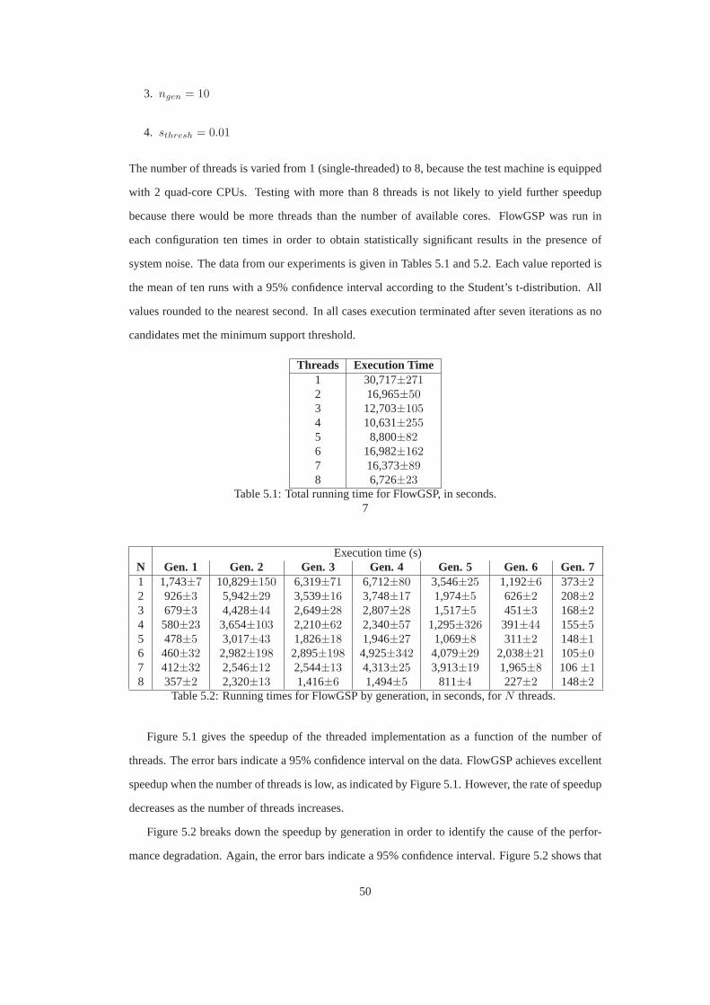
3. ngen = 10
4. sthresh = 0.01
The number of threads is varied from 1 (single-threaded) to 8, because the test machine is equipped
with 2 quad-core CPUs. Testing with more than 8 threads is notlikely to yield further speedup
because there would be more threads than the number of available cores. FlowGSP was run in
each configuration ten times in order to obtain statistically significant results in the presence of
system noise. The data from our experiments is given in Tables 5.1 and 5.2. Each value reported is
the mean of ten runs with a 95% confidence interval according to the Student’s t-distribution. All
values rounded to the nearest second. In all cases executionterminated after seven iterations as no
candidates met the minimum support threshold.
Threads Execution Time1 30,717±2712 16,965±503 12,703±1054 10,631±2555 8,800±826 16,982±1627 16,373±898 6,726±23
Table 5.1: Total running time for FlowGSP, in seconds.7
Execution time (s)N Gen. 1 Gen. 2 Gen. 3 Gen. 4 Gen. 5 Gen. 6 Gen. 71 1,743±7 10,829±150 6,319±71 6,712±80 3,546±25 1,192±6 373±22 926±3 5,942±29 3,539±16 3,748±17 1,974±5 626±2 208±23 679±3 4,428±44 2,649±28 2,807±28 1,517±5 451±3 168±24 580±23 3,654±103 2,210±62 2,340±57 1,295±326 391±44 155±55 478±5 3,017±43 1,826±18 1,946±27 1,069±8 311±2 148±16 460±32 2,982±198 2,895±198 4,925±342 4,079±29 2,038±21 105±07 412±32 2,546±12 2,544±13 4,313±25 3,913±19 1,965±8 106±18 357±2 2,320±13 1,416±6 1,494±5 811±4 227±2 148±2
Table 5.2: Running times for FlowGSP by generation, in seconds, forN threads.
Figure 5.1 gives the speedup of the threaded implementationas a function of the number of
threads. The error bars indicate a 95% confidence interval onthe data. FlowGSP achieves excellent
speedup when the number of threads is low, as indicated by Figure 5.1. However, the rate of speedup
decreases as the number of threads increases.
Figure 5.2 breaks down the speedup by generation in order to identify the cause of the perfor-
mance degradation. Again, the error bars indicate a 95% confidence interval. Figure 5.2 shows that
50

0
1
2
3
4
5
0 1 2 3 4 5 6 7 8
Spe
edup
Number of Threads, N
Figure 5.1: Total speedup as a function of the number of threadsN .
we obtained similar speedups on all iterations of the algorithm. Therefore we cannot isolate any
particular iteration or iterations as a cause of the poor speedup in later generations.
Figure 5.2 also shows that when the algorithm is run with 6 or 7threads the speedup obtained is
extremely poor. The machine used for these performance runsis a part of a cluster of machines; it
is possible that other nodes on the cluster experienced increased use during this period. Other nodes
being used would effect the results of this experiment as allnetwork traffic from each node is routed
through a single master node. It is also possible that increased network congestion at the time of the
experiment could infuence the execution time of the algorithm because the database server is hosted
on a seperate machine. However, a repeated run of the algorithm with 7 threads again produced data
consistent with the observations in Table 5.1. Therefore itis unclear exactly what is causing this
particular performance anomaly.
Time (in seconds)Generation Mining Fetching Pruning/Joining
1 338 19 02 2302 18 0.23 1394 20 0.14 1476 18 0.15 793 18 06 209 18 07 130 18 0
Table 5.3: Breakdown of execution time with 8 worker threads.
Table 5.3 breaks down the time spent mining each generation into three sections: time spent
mining, time spent fetching data from the database, and timespent pruning and creating the next
generation for 8 threads. The amount of time spent fetching data from the database is uniform
accross all iterations of the algorithm. There is also a noticible increase in the amount of time spent
51
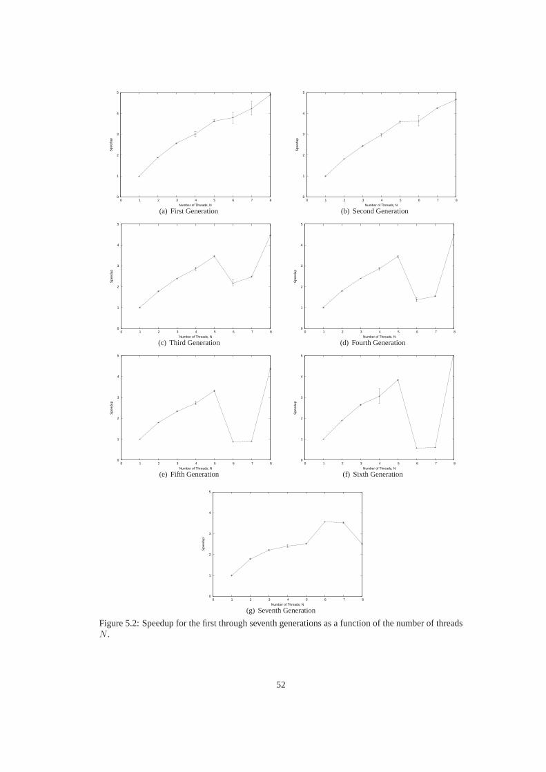
0
1
2
3
4
5
0 1 2 3 4 5 6 7 8
Spe
edup
Number of Threads, N
(a) First Generation
0
1
2
3
4
5
0 1 2 3 4 5 6 7 8
Spe
edup
Number of Threads, N
(b) Second Generation
0
1
2
3
4
5
0 1 2 3 4 5 6 7 8
Spe
edup
Number of Threads, N
(c) Third Generation
0
1
2
3
4
5
0 1 2 3 4 5 6 7 8
Spe
edup
Number of Threads, N
(d) Fourth Generation
0
1
2
3
4
5
0 1 2 3 4 5 6 7 8
Spe
edup
Number of Threads, N
(e) Fifth Generation
0
1
2
3
4
5
0 1 2 3 4 5 6 7 8
Spe
edup
Number of Threads, N
(f) Sixth Generation
0
1
2
3
4
5
0 1 2 3 4 5 6 7 8
Spe
edup
Number of Threads, N
(g) Seventh Generation
Figure 5.2: Speedup for the first through seventh generations as a function of the number of threadsN .
52

Gap Size Window Size Execution Time (s)0 0 6,7260 1 14,0681 0 12,7481 1 22,314
Table 5.4: Influence of changing gap and window sizes on overall program performance.
pruning and joining the next generation of candidates, but this accounts for a small portion of total
execution time.
The amount of time spent fetching data from the database is measured by starting and stopping
a timer around each JDBC call, summing the time for all such calls from the same thread, and then
averaging the totals over all worker threads. The amount of time spent pruning/joining is measured
by a similar timer in the master thread. The time spent pruning/joining also includes the time spent
fetching results from the worker threads. The time reportedas mining time is the difference between
the time for the mining task and the sum of the fetching and pruning/joining time.
The runs which produced the data in Tables 5.1 and 5.2 were obtained with a gap size of zero
and a window size of zero. In many datasets a larger gap or window size may be required in order to
discover interesting sequences. Table 5.4 shows the running time of FlowGSP on a Websphere Ap-
plication Server profile when the gap and window sizes are increased. For this experiment FlowGSP
was again run with 8 threads for ten iterations with a supportthreshold of 1%.
Increasing either the gap or the window size results in a significant increase in execution time.
This increase can be explained by a general increase in the support values of candidate sequences and
consequently more candidates meeting the support threshold. More candidates meeting the support
threshold results in more candidates being generated at each iteration. Based on this data, it may be
prudent to increase the support threshold when running FlowGSP with non-zero gap and window
sizes in order to control the execution time. However, whileincreasing the support threshold is a
good idea for Application Server profiles, this decision is ultimately dependant on the characteristics
of the data being mined.
5.3 Distributed Implementation
This section describes a socket-based version of the algorithm for use in distributed memory ma-
chines. The scalability of the threaded implementation is limited by the number of cores on a single
machine1. In order for the distributed implementation to be of use, itmust scale beyond the capabil-
ities of the threaded implementation. The distributed implementation described in this section does
1Most standard Java Virtual Machines (JVMs) do not allow for the distribution of threads between multiple machines.
53
not scale, therefore there is little reason to deploy this implementation of FlowGSP on a large cluster
as opposed to single multi-core workstations.
5.3.1 Work Division
Similar to the threaded implementation, work is divided by asingle master. Each worker is as-
signed an equal-sized subset of the candidate sequences in the current generation. Each worker then
searches for instances of its subset of candidates over all of the methods in the profile. The deci-
sion to divide work in this manner was made after an initial attempt that divided work in the same
manner as the threaded version. Information that needs to betransmitted from the master to the
workers incurs a communication overhead because each worker has its own private address space.
The amount of overhead for early generations is small because there are few candidates, but in later
generations copying all candidates to each client is prohibitively expensive. Collecting results from
workers is even more expensive: not only do the candidates need to be copied from each worker
but the supports found by each worker need to be merged. Therefore, the method of work division
was changed to reduce both the communication between workers and the computation needed to
combine results from clients.
The only other difference between the socketed and threadedimplementations is that the work-
ers in the socketed implementation prune candidates with inadequate support prior to communicat-
ing the results of the mining to the master worker. This optimization was not implemented in the
threaded version because all workers search for instances of all candidate sequences, therefore any
pruning must wait until all workers have finished. This limitation is not present given this work dis-
tribution scheme and therefore it was convenient to implement this advanced pruning. It is unlikely,
however, that this optimization resulted in any significantperformance improvement.
5.3.2 Performance Analysis
The socketed implementation demonstrates extremely poor performance. In fact, runs with more
than 2 workers usually resulted in a significant slowdown compared to the sequential case (in this
instance, a run of the socketed implementation with only oneworker apart from the master).
Table 5.5 gives the execution times for the distributed implementation for 1,2,4,8, and 16 work-
ers. The data in Table 5.5 is from a single run of the distributed implementation and therefore may
contain a significant amount of error. However, given that the distributed implementation fails to
even achieve a speedup of two with sixteen workers, no further runs were performed and a 95%
54

Execution Time (in seconds)N Gen. 1 Gen. 2 Gen. 3 Gen, 4 Gen. 5 Total1 697 1,434 2,240 6,666 10,437 21,4782 455 975 1,673 4,565 7,345 15,0184 370 625 1,313 4,986 9,088 16,3888 506 556 1,016 5,199 10,696 17,97816 684 647 816 3,974 11,178 17,304
Table 5.5: Execution time for the distributed implementation of FlowGSP withN workers.
confidence interval was not calculated. It is unlikely that the amount of error represents more than a
small portion of total execution time.
In order to understand the behavior of the distributed implementation, the amount of time spent
fetching data from the database was recorded. The time spentfetching data was recorded in the same
manner as the threaded implementation. The data shows that,for 16 workers, 1,688 seconds were
spent fetching data from the database. It is unlikely that the fetching of data from the database is the
bottleneck for the distributed implementation because theamount of time spent fetching accounts
for only 9.7% of total execution time.
The amount of time spent retrieving results from workers, pruning candidates with insufficient
support, and creating the next generation of candidates wasalso recorded. The amount of time spent
on these activities accounts for twelve seconds. Twelve seconds is a relatively insignificant portion
of the total execution time listed in Table 5.5.
It seems likely that poor granularity is the reason the distributed implementation experiences
poor performance. The current method of work division was implemented only after the work-
division scheme used in the threaded implementation was used unsuccessfully. Neither of these
methods of work division result in good parallel performance. Therefore further work is required
to determine an appropriate method of dividing the mining problem among the workers. Given the
relatively good performance of the threaded implementation, the discovery of such a method is left
to future work.
Final Remarks
A threaded and distributed (via sockets) implementation of FlowGSP has been discussed. The
threaded version achieved a 78% decrease in total executiontime. The threaded implementation
of FlowGSP reduces execution time to the point where multiple runs can be easily performed in a
day, a critical feature if FlowGSP is to be used in a production compiler environment. It may be pos-
sible with further investigation to further increase the performance of the threaded implementation.
55

The distributed version, unfortunately, achieves little to no speedup because the database server
is unable to cope with the volume or frequency of requests. Itis possible that with more resources the
performance of both implementations of FlowGSP could see significant improvement. The socketed
implementation is of no use because it is outperformed by thethreaded implementation.
56

Chapter 6
Mining WebSphere Application
Server Profiles with FlowGSP
The experimental results presented in this Chapter demonstrate that FlowGSP works in the context of
mining WebSphere Application Server profiles, a large enterprise application. The execution paths
in this server consist of millions of assembly instructionsper transaction and a plethora of hardware
events per instruction. These results establish FlowGSP asa practical and effective solution for the
mining of large flow graphs.
6.1 Discovery of Previously Known Patterns
Before the development of FlowGSP, compiler developers were faced with the difficult challenge
of identifying patterns in the execution paths of large enterprise applications using nothing but in-
tuition and observation. This approach to discovery is not only tedious and time consuming, but is
also fraught with limitations of capturing the scope and respective support for improvement oppor-
tunities. The intuitive approach may lead to large investments in compiler development effort that
may not necessarily pay off. Countless person-hours of effort have been invested in such discovery
processes.
With the implementation of FlowGSP, an interesting acid test of the automatic approach is to dis-
cover patterns that had already been identified manually by compiler developers. FlowGSP passed
this acid test because it was able to identify all the patterns that were known to the developers. Some
of these patterns include:
57
• 〈(Icachemiss, TLBmiss)〉, SM = 0.529 indicates a high correlation between instruction-
cache misses and TLB misses on the host architecture.
• 〈(Prologue, Icachemiss)〉, SM = 0.1175 indicates a high occurrence of instruction-cache
misses in the prologues of methods. This is significant considering that the sequence
〈(Prologue)〉 hasSM = 0.120.
• 〈(JIT target, Icachemiss)〉, SM = 0.0935 corresponds to a significant number of instruction-
cache misses on the JIT target instructions. The JIT target instruction is the first assembly in-
struction to be called when the method is called from natively compiled code. In general, a dif-
ferent first instruction is executed when the method is called from interpreted code. The level
of support for this attribute pair is even more significant because the sequence〈(JIT target)〉
hasSM = 0.0935.
6.2 Discovery of New Characteristics
In addition to re-discovering known patterns, FlowGSP was effective in identifying an opportunity
to improve WebSphere Application Server performance by enabling large pages. By discovering a
high incidence and correlation of instruction cache and TLBmisses, FlowGSP helped identify the
use of large pages as a performance opportunity. As such, enabling large pages resulted in a 3-4%
decrease in instruction-cache misses and an overall throughput improvement of 2%.
FlowGSP was also successful at discovering many expected patterns. For instance, it is known
that the instruction-cache-miss counter exhibits a long tail because the counter continues to register
for multiple instructions following the instruction that incurred the actual delinquent cache fetch.
FlowGSP identified good support for the sequence〈(Icachemiss), (Icachemiss)〉, SM = 0.112.
A result that confirms thisa priori knowledge. FlowGSP also identified a high occurance of se-
quences which contained data cache misses and TLB misses, a result that is both typical and ex-
pected.
The sequence〈(Icachemiss,Branchmispredict)〉, SM = 0.240 shows that there is a corre-
lation between branch mispredictions and instruction-cache misses. This observation suggests that
it may be possible to improve the hardware’s branch predictor to improve WebSphere Application
Server performance.
58
Final Remarks
This chapter demonstrated that FlowGSP is able to identify known patterns in an EFG constructed
from a WebSphere Application Server profile. These patternswere identified with a level of support
proportional to their known significance. This chapter alsoshowed that FlowGSP is capable of
identifying previously unknown sequences in an EFG, and that these sequences can be used to
achieve performance improvements in the target application.
59

60

Chapter 7
Related Work
There has been a significant body of work recently investigating the possible applications of machine
learning techniques to compiler research. The applicationof machine learning could potentially
relieve many person-hours of intensive, skilled labor because compilers rely heavily on hand-tuned
heuristics. Section 7.1 discusses such applications.
Data mining techniques have been extended to mine data in a large variety of formats. While, to
the best of our knowledge, no algorithm exists that can mine EFGs, there are a number of algorithms
that mine similar types of data. These algorithms are discussed in Section 7.2.
There have also been a number of efforts to improve compiler performance through traditional
means based on hardware profiling information. Section 7.3 discusses some of these approaches.
Enterprise applications, such as the WebSphere Application Server, usually carry a very large
load in terms of responsibility for many businesses. Therefore, interest in improving their per-
formance is common. Other approaches that attempt to improve the performance of large Java
applications are covered in Section 7.4.
While all of these approaches have some elements in common with FlowGSP, none of them are
uniquely equipped to handle the challenges faced when mining for frequent sequences in hardware
profile data.
7.1 Machine Learning and Compilers
A common problem with trying to achieve optimal performancewith modern optimizing compilers
is that it is extremely difficult to predict the ideal optimization parameters for any given program.
Moreover, the number of possible parameter values for most optimizing compilers is extremely
61

large. Manually searching through them all,i.e. through iterative optimization, is prohibitively
expensive. Compiler researchers have begun to turn to the field of machine learning in order to more
efficiently find good optimization configurations.
7.1.1 Supervised Learning
There have been a number of efforts into using predictive models to improve the performance of
optimizing compilers.
Cavazoset. al. present a method for automatically selecting good compileroptimizations via
a model constructed using performance-counter data [6]. They evaluate a variety of optimization
configurations on a training set of programs and use the resulting speedups relative to a baseline
optimization level to construct a predictive model. Given anovel program, they compile it once
using the baseline compiler options. The performance-counter data from this run is fed back into
the model to produce a set of “best” optimizations. They testtheir system using cross-validation
on the PathScale EKOPath compiler and the Standard Performance Evaluation Corporation (SPEC)
1995 benchmark suite. N-fold Cross-validation involves splitting the data set into N sections, then
training on N-1 sections and testing on the remaining section. Cavazoset. al. are able to achieve a
17% performance increase over the fastest built-in optimization setting (-Ofast). While they do
produce excellent results, they are only exploring the space of all pre-existing optimization settings.
FlowGSP allows the discovery of new opportunities for code transformations that may not be within
the scope of existing compiler flags. It would not be possiblefor their system to discover any of
these opportunities.
Stephensonet al. use supervised learning techniques to determine the ideal loop unrolling factor
for a program [33]. They use both nearest-neighbor and Support Vector Machine (SVM) classifiers
[9] in their research. Using these methods they are able to improve loop unrolling performance by
5% on the SPEC 2000 benchmark suite [8]. While an adapted version of their tool could be used
to discover good parameter values for existing optimization, their method is unable to discover
opportunities for new code transformations, or even if the current set of parameters to existing
options is wanting.
7.1.2 Unsupervised Learning
Stephensonet al. (2003) use Genetic Programming to determine ideal parameters for hyperblock
formation, data prefetching, and register allocation [34]. Genetic Programming uses the principles
62

of genetics to “evolve” more suitable candidates over multiple generations. However there is some
doubt as to the usefulness of genetic algorithms in cases such as these, especially when their perfor-
mance is compared to that of pure random search [4].
7.2 Data Mining
Mining for frequent sequences in structured data has its roots in algorithms such as GSP [2], PrefixS-
pan [13], and WINEPI/MINEPI [20]. These algorithms all search for sequences or partial sequences
within a totally ordered dataset. While this assumption of a total ordering is sufficient for some ap-
plications, such as market-basket analysis, there are manyexamples of real-world data, such as
hardware profiles, that cannot be expressed using a total ordering.
One of the most commonly used data structures in both computing science and mathematics is a
graph. It should come as no surprise that there has been a significant amount of work devoted toward
developing mining algorithms that operate on topologically ordered data structures such as graphs.
AGM [16], gSpan [39], Origami [14], and Gaston [23] are all algorithms that search for frequent
substructures in graph-based data.
While mining for common substructures is a very similar goal to that accomplished by FlowGSP,
there are some crucial differences. First, FlowGSP is interested in discovering frequent sequences
of attributes on the vertices of a flow graph. The mining performed by FlowGSP is more than just
frequent substructure discovery because a frequent connected substructure need not be a sequence
of vertices. Also, none of the cited works handle multiple labels or attributes on vertices.
A traversal of a graph is an ordered sequence of connected vertices in a graph. There are a num-
ber of real-world situations for which finding frequent sequences in a collection of graph traversals
may prove useful, such as analyzing the behavior of visitorsto a web site.
Lee et al.develop an algorithm for discovering frequent patterns in traversals of a weighted,
directed graph [19]. A traversal of a graph is an ordered sequence of connected vertices in the
underlying graph. They evaluate their algorithm on a numberof randomly generated graphs.
Genget al. propose another algorithm for mining frequent patterns in traversals of graphs with
weighted edges and vertices [11]. They used a generate-and-test approach based on the Apriori
algorithm [30] to grow their candidate patterns.
The key difference between these traversal-mining algorithms and FlowGSP is the form of the
data being mined. Both Leeet al. and Genget al. mine a collection of traversals over a graph. This
difference is illustrated by Figure 7.1. Subfigure (a) is an example of a directed graph G; subfigure
63

(b) gives a list of weighted traversals. Each traversal consists of a sequence of nodes from G (under
the traversal column) and a series of weights assigned to each edge of the traversal (under the weight
column). This figure is adapted from Figure 1 in [19]. Traversals such as these are not the same as
the EFGs mined by FlowGSP: FlowGSP mines for frequent possible subpaths in a graph.
D B
A
CE
(a) G
ID Traversal Weight1 < A,B,C > < 2.2, 2.0 >2 < B,D,E,C,A > < 3.0, 4.3, 3.5, 3.1 >3 < C,A,B,D > < 2.9, 2.0, 4.0 >4 < D,C,A > < 4.0, 3.0 >5 < B,C,A > < 2.2, 2.9 >6 < A,B,E,C > < 1.4, 3.9, 4.4, 3.2 >
(b) Traversals on G
Figure 7.1: Example of a directed graph and a weighted traversal.
Hwanget al. perform data mining on program call graphs in order to identify recurring pat-
terns in method call sequences [15]. They successfully identify two commonly occurring “control
patterns” that occur frequently together in a collection ofJava programs. Hwanget al. only pro-
vide the mechanism for identifying these control patterns and do not provide insights into how this
information may be used to increase program performance. Also, their work relies on obtaining pro-
gram traces rather than profiles. The cost of obtaining a fulltrace for an application as large as the
WebSphere Application Server would be prohibitively expensive. Their method also only uses the
sequence of method calls and does not incorporate low-levelor performance-counter information.
Pawlak develops a method for mining association rules from labelled, weighted, flow graphs
[24]. They derive these rules by “fusing” the graph being mined and combining the normalized
edge weights. Through fusing they are able to obtain association rules between the graph’s sources
and sinks by fusing out all the intermediary nodes. Such an approach does not map well to mining
control-flow-graph data because each method has only a single source and single sink node. Also,
patterns that occur within the internal structure of a flow graph are of higher interest.
Moseleyet al. develop Optiscope, a tool for comparing multiple hardware profiles [21]. Their
goal is to allow easy comparison of multiple executions of the same program under various compiler
configurations. Loops in each profile are matched, and the differences in the profiling information
examined via a web interface. The profiling data from each loop or method is aggregated and
compared. The local focus of Optiscope is in sharp contrast to the goal of finding global patterns
that may yield performance opportunities. Optiscope is built around basic slicing operations. That is
64

to say that optiscope only performs basic aggregations; no search for frequent patterns or sequences
is performed.
7.3 Performance Counters
Choi et al. use performance counter data to enhance the performance of the Intel compiler on the
Itanium 2 platform [7]. They use performance counter data tosupplement the information usually
obtained during static FDO. However, as is usual for FDO, their process is restricted to improv-
ing the performance of existing code transformations and cannot aid in the discovery of new code
transformations.
There have been a growing body of research directed towards allowing JIT compilers access to
hardware profiling data at run-time. Schneideret al. collects information about instruction cache
misses on the Intel Pentium 4 platform in order to increase performance via object co-allocation [27].
Cuthbertsonet al. also use I-cache information from hardware event counters on the Intel Itanium
platform to improve co-allocation, as well as to influence global scheduling [10]. Shyeet al. collect
branching information from the Itanium Branch Transition Buffer (BTB) and use this information to
build partial path profiles of the executing program [28]. All of these works only operate on a very
small number of performance counters. While a small number ofcounters is enough data for the
code transformations they investigate, by discarding someperformance counters, information about
the program is lost. It may not be possible to simply increasethe amount of counter information
passed into the JVM, because it is not clear how well the strategies presented will scale as the number
of counters retrieved increases.
Buytaertet al. use hardware-performance counters (in particular sampling ticks) to increase
the accuracy and decrease the cost of the instrumentation used to detect hot methods in a Java
JIT compiler [5]. No new code transformations are introduced because their work is focused on
improving the performance of current techniques.
7.4 Enterprise Application Performance
Xu et al. investigate object copying as a symptom of bloat in large Java applications [38]. By
profiling object copy behavior they are able to hand-tune their applications and significantly increase
performance. They are able to decrease the execution time oftwo DaCapo benchmarks by 65% and
9.3% respectively. While Xuet al. also investigate large scale Java application performancetheir
65
approach is focused on hard tuning the resulting application instead of searching for opportunities for
new compiler code optimizations. While application tuning is important for overall performance, the
role of the compiler is equally important. FlowGSP addresses the needs of the compiler developer
when it comes to improving the performance of enterprise applications.
66
Conclusion
This thesis presented the EFG, a data structure that represents the information contained in hardware
profiles. This data structure was designed by supplementingthe profile data with the CFG taken from
the compiler logs. This thesis defined the notions of frequency and weight support of a subpath in
an EFG. It also presented FlowGSP, an algorithm to mine for sequences in an EFG. FlowGSP ranks
sequences by both their frequency in the graph and by the costof the subpaths in which they appear.
EFGs were constructed using profiling information obtainedfrom WebSphere Application Server
runs on the IBM z10 architecture. A list of attributes was created to represent the characterstics of
z10 profiling data. This thesis presented an implementationof FlowGSP in Java to mine these EFGs.
Two parallel implementations of FlowGSP were also introduced. The first implementation uses
Java threads and is targeted at the rapidly growing domain ofmulti-core workstations. The threaded
implementation of FlowGSP reduces the time required to minea profile of the WebSphere Appli-
cation Server by roughly 75%. This improved performance allows FlowGSP to mine such a profile
many times in a day, a necessary requirement for deployment in a production compiler develop-
ment environment. This thesis also presented a distributedimplementation of FlowGSP targeted at
cluster-based computing. However, the distributed implementation failed to show the performance
necessary to merit deployment. Future work may yield a better work-division strategy for this im-
plementation.
FlowGSP was evaluated on WebSphere Application Server hardware profiles. This thesis pre-
sented a number of sequences discovered by FlowGSP which characterize known Application Server
behavior. The discovery of previously unknown sequences was also discussed. These new sequences
may yield new performance opportunities upon further study.
There are a number of areas for future development based on the work in this thesis. The parallel
implementations of FlowGSP discussed in Chapter 5 can be greatly improved. The threaded imple-
mentation suffers from a database bottleneck. Adding additional database servers or implementing
some caching protocol may alleviate this bottleneck. The distributed implementation exhibits poor
67

granularity and does not scale to a large number of nodes. Thedevelopment of an alternate method
of work division which does not exhibit this poor granularity would increase the viability of this
implementation.
There are a number of newer data mining algorithms, PrefixSpan [25] for example, that have
improved performance compared to GSP. GSP was chosen as the basis for FlowGSP due to its
simplicity and the fact that it is well studied. Other sequence-mining algorithms could be extended to
achieve the same goals as FlowGSP, perhaps with greater efficiency. It may also be possible to extend
a graph mining algorithm such as Gaston [23] or gSpan [39] to search for frequent sequences in an
EFG. These algorithms have differing characteristics and it is possible that using an algorithm other
than GSP as the base to mine EFGs for data may result in considerable performance improvements.
FlowGSP has been extensively tested on WebSphere Application Server profiles. However, the
WebSphere Application Server is hardly representative of all programs. Other application profiles
could yield patterns of interest to compiler developers with FlowGSP’s help.
EFGs are not limited to hardware profiles. There are many other domains that could be charac-
terized in a manner similar to performance-counter data. Web traffic pattern analysis, urban traffic
planning, and purchasing pattern analysis are examples of areas that could benefit from the applica-
tion of FlowGSP.
68
Bibliography
[1] WebSphere Application Server. http://www-01.ibm.com/software/websphere/, March 2009.
[2] Rakesh Agrawal and Ramakrishnan Srikant. Mining sequential patterns. InInternational
Conference on Data Engineering (ICDE), pages 3–14. IEEE Computer Society, March 1995.
[3] Enrique Alba. Parallel evolutionary algorithms can achieve super-linear performance.Inf.
Process. Lett., 82(1):7–13, 2002.
[4] Jose Nelson Amaral, Adalberto Tiexeira Castelo Neto, and Alessandro Valerio Dias. Genetic
algorithms in optimization: Better than random search? In1997 International Conference on
Engineering and Informatics, pages 320–326, April 1997.
[5] Dries Buytaert, Andy Georges, Michael Hind, Matthew Arnold, Lieven Eeckhout, and Koen
De Bosschere. Using HPM-sampling to drive dynamic compilation. volume 42, pages 553–
568. ACM, 2007.
[6] John Cavazos, Grigori Fursin, Felix Agakov, Edwin Bonilla, Michael F. P. O’Boyle, and Olivier
Temam. Rapidly selecting good compiler optimizations using performance counters. InCode
Generation and Optimization (CGO), pages 185–197, Washington, DC, USA, 2007. IEEE
Computer Society.
[7] Y. Choi, A. Knies, G. Vedaraman, and J. Williamson. Design and experience using the Intel
Itanium 2 processor performance monitoring unit to implement feedback optimizations.EPIC2
Workshop, 2002.
[8] Standard Performance Evaluation Corporation. SPEC benchmark. http://www.spec.org.
[9] Koby Crammer and Yoram Singer. On the algorithmic implementation of multiclass kernel-
based vector machines.J. Mach. Learn. Res., 2:265–292, 2002.
69

[10] John Cuthbertson, Sandhya Viswanathan, Konstantin Bobrovsky, Alexander Astapchuk, and
Eric Kaczmarek. Uma Srinivasan. A practical approach to hardware performance monitoring
based dynamic optimizations in a production JVM. InCode Generation and Optimization
(CGO), pages 190–199, Seattle, WA, USA, 2009. IEEE Computer Society.
[11] Runian Geng, Xiangjun Dong, Xingye Zhang, and Wenbo Xu.Efficiently mining closed fre-
quent patterns with weight constraint from directed graph traversals using weighted FP-tree
approach. InInternational Colloquium on Computing, Communication, Control, and Manage-
ment, pages 399–403, Guangzhou City, China, August 2008.
[12] M. Golden and T. Mudge. Comparison of two common pipeline structures.Computers and
Digital Techniques, IEE Proceedings, 143(3):161–167, May 1996.
[13] J. Han, J. Pei, and Y. Yin.Sequential Pattern Mining by Pattern-Growth: Principles and
Extensions, volume 180 ofStudies in Fuzziness and Soft Computing, pages 183–220. Springer,
2005.
[14] Mohammad Al Hasan, Vineet Chaoji, Saeed Salem, Jeremy Besson, and Mohammed J. Zaki.
Origami: Mining representative orthogonal graph patterns. In International Conference on
Data Mining (ICDM), pages 153–162, Omaha, NE, USA, 2007. IEEE Computer Society.
[15] Chung-Chien Hwang, Shih-Kun Huang, Deng-Jyi Chen, andD.T.K. Chen. Object-oriented
program behavior analysis based on control patterns. InAsia-Pacific Conference on Quality
Software (APCQS), pages 81–87, Hong Kong, China, December 2001.
[16] Akihiro Inokuchi, Takashi Washio, and Hiroshi Motoda.An apriori-based algorithm for min-
ing frequent substructures from graph data. InPKDD ’00: Proceedings of the 4th European
Conference on Principles of Data Mining and Knowledge Discovery, pages 13–23, London,
UK, 2000. Springer-Verlag.
[17] K.M. Jackson, M.A. Wisniewski, D. Schmidt, U. Hild, S. Heisig, P. C. Yeh, and W. Gellerich.
IBM system z10 performance improvements with software and hardware synergy.IBM J. Res.
Dev., 53(1-16), May 2009.
[18] T. Kisuki, P.M.W. knijnenburg, Michael F. P. O’Boyle, Francois Bodin, and E. Rouhu. Iterative
compilation in a non-linear optimization space. InParallel Architectures and Compilation
Techniques (PACT), Paris, France, October 1998.
70

[19] Seong Dae Lee and Hyu Chan Park. Mining frequent patterns from weighted traversals on
graph using confidence interval and pattern priority.International Journal of Computer Science
and Network Security (IJCSNS), 6(5A):136–141, May 2006.
[20] H. Mannila, H. Toivonen, and A. I. Verkamo. DiscoveringFrequent Episodes in Sequences.
In U. M. Fayyad and R. Uthurusamy, editors,Knowledge Discovery and Data Mining (KDD),
Montreal, Canada, 1995. AAAI Press.
[21] Tipp Moseley, Dirk Grunwald, and Ramesh V. Peri. Optiscope: Performance accountability
for optimizing compilers. InCode Generation and Optimization (CGO), Seattle, WA, USA,
2009. IEEE Computer Society.
[22] Priya Nagpurkar, Harold W. Cain, Mauricio Serrano, Jong-Deok Choi, and Ra Krintz. A study
of instruction cache performance and the potential for instruction prefetching in J2EE server
applications. InWorkshop of Computer Architecture Evaluation using Commercial Workloads
(CAECW), Phoenix, AZ, USA, 2007.
[23] Siegfried Nijssen and Joost N. Kok. A quickstart in frequent structure mining can make a
difference. InKnowledge Discovery and Data Mining (KDD), pages 647–652, New York, NY,
USA, 2004. ACM.
[24] Zdzislaw Pawlak. Flow graphs and data mining. InTransactions on Rough Sets III, volume
3400/2005 ofLecture Notes in Computing Science, pages 1–36. Springer, 2005.
[25] J. Pei, J. Han, B. Mortazavi-Asl, H. Pinto, Q. Chen, U. Dayal, and M.C. Hsu. PrefixSpan
mining sequential patterns efficiently by prefix projected pattern growth. InInternational Con-
ference on Data Engineering (ICDE), pages 215–226, Heidelburg, Germany, 2001.
[26] K.E. Plambeck, W. Eckert, R. R. Rogers, and C. F. Webb. Development and attributes of
z/architecture.IBM J. R. Dev., 46(4-5):367, 2002.
[27] Florian T. Schneider, Mathias Payer, and Thomas R. Gross. Online optimizations driven by
hardware performance monitoring. InProgramming language design and implementation
(PLDI), pages 373–382, New York, NY, USA, 2007. ACM.
[28] Alex Shye, Matthew Iyer, Tipp Moseley, David Hodgdon, Dan Fay, Vijay Janapa Reddi, and
Daniel A. Connors. Analyis of path profiling information generated with performance moni-
toring hardware. InWorkshop on Interaction between Compilers and Computer Architectures
(INTERACT), pages 34–43, Rome, Italy, 2005. IEEE Computer Society.
71
[29] T. J. Siegel, E. Pfeffer, and J. A. Magee. The IBM eServerz990 microprocessor.IBM J. Res.
Dev., 48(3-4):295–309, 2004.
[30] Ramakrishnan Srikant and Rakesh Agrawal. Mining quantitative association rules in large
relational tables. InSIGMOD International Conference on Management of Data, pages 1–12,
New York, NY, USA, 1996. ACM.
[31] Ramakrishnan Srikant and Rakesh Agrawal.Mining Sequential Patterns: Generalizations and
Performance Improvements, pages 3–17. Advances in Database Technology. Springer, 1996.
[32] Ramakrishnan Srikant and Rakesh Agrawal. Mining sequential patterns: Generatlizations and
performance improvements. Technical report, IBM ResearchDivision, Almaden Research
Center, San Jose, CA, USA, 1996.
[33] Mark Stephenson and Saman Amarasinghe. Predicting unroll factors using supervised classi-
fication. InCode Generation and Optimization (CGO), pages 123–134, San Jose, CA, USA,
2005. IEEE Computer Society.
[34] Mark Stephenson, Saman Amarasinghe, Martin Martin, and Una-May O’Reilly. Meta opti-
mization: improving compiler heuristics with machine learning. In Programming language
design and implementation (PLDI), pages 77–90, New York, NY, USA, 2003. ACM.
[35] Robert Tibshirani and Jerome Friedman Trevor Hastie.The Elements of Statistical Learning:
Data Mining, Inference, and Prediction. Springer, New York, 2001.
[36] E. Tzortzatos, J. Bartik, and P. Sutton. IBM system z10 support for large pages.IBM J. Res.
Dev., 53(1-17), May 2009.
[37] C. F. Webb. IBM z10: The next generation microprocessor. IEEE Micro, 28(2):19–29, March
2008.
[38] Guoqing Xu, Matthew Arnold, Nick Mitchell, Atanas Rountev, and Gary Sevitsky. Go with
the flow: profiling copies to find runtime bloat. InPLDI ’09: Proceedings of the 2009 ACM
SIGPLAN conference on Programming language design and implementation, pages 419–430,
Dublin, Ireland, 2009. ACM.
[39] Xifeng Yan and Jiawei Han. gSpan: Graph-based substructure pattern mining. InInternational
Conference on Data Mining (ICDM), page 721, Maebashi City, Japan, 2002. IEEE Computer
Society.
72