Northwest Advanced Renewables Alliance

Douglas-fir biomass and nutrient removal under varying harvest intensities designed for co-production of timber and biofuel

Kristin Coons, Doug Maguire, Doug Mainwaring, Andy Bloom, Rob Harrison, and Eric Turnblom

http://liferefocused.wordpress.com/

Background• Biofuel is a viable, renewable

alternative to fossil fuels.

• The leading national level assessment proposes displacing 30% of the petroleum consumed in the U.S.

• Biofuel produced from forests comprises 50% of energy derived from all biomass in the U.S.

• The majority of aboveground biomass in the PNW is Douglas-fir.

OutlineI. Background

II. Objectives

III. Hypotheses

IV. Study Sites

V. Methods

VI. Preliminary Results

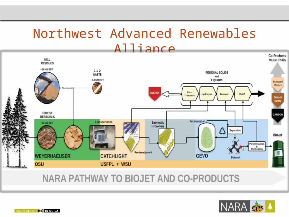
Northwest Advanced Renewables Alliance

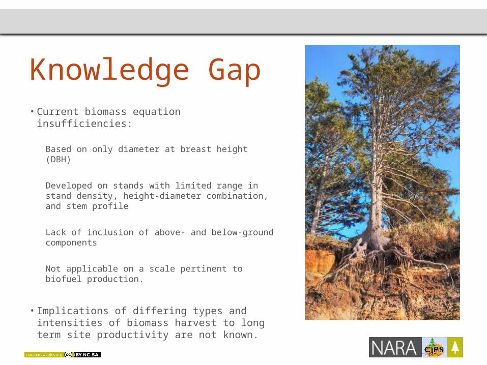
Knowledge Gap• Current biomass equation insufficiencies:

­ Based on only diameter at breast height (DBH)

­ Developed on stands with limited range in stand density, height-diameter combination, and stem profile

­ Lack of inclusion of above- and below-ground components

­ Not applicable on a scale pertinent to biofuel production.

• Implications of differing types and intensities of biomass harvest to long term site productivity are not known.

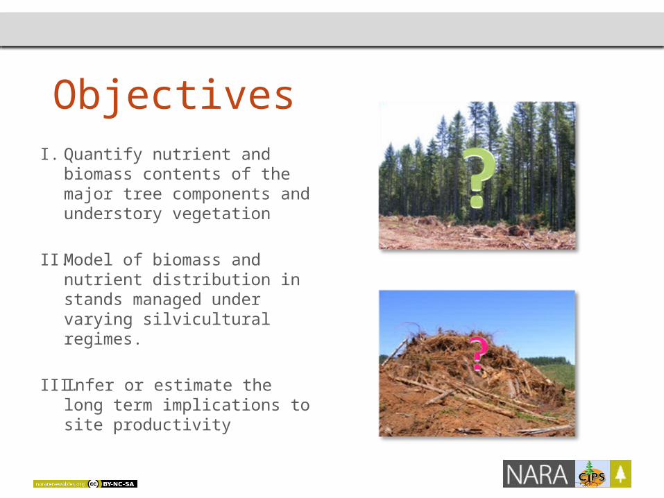
ObjectivesI. Quantify nutrient and

biomass contents of the major tree components and understory vegetation

II. Model of biomass and nutrient distribution in stands managed under varying silvicultural regimes.

III. Infer or estimate the long term implications to site productivity

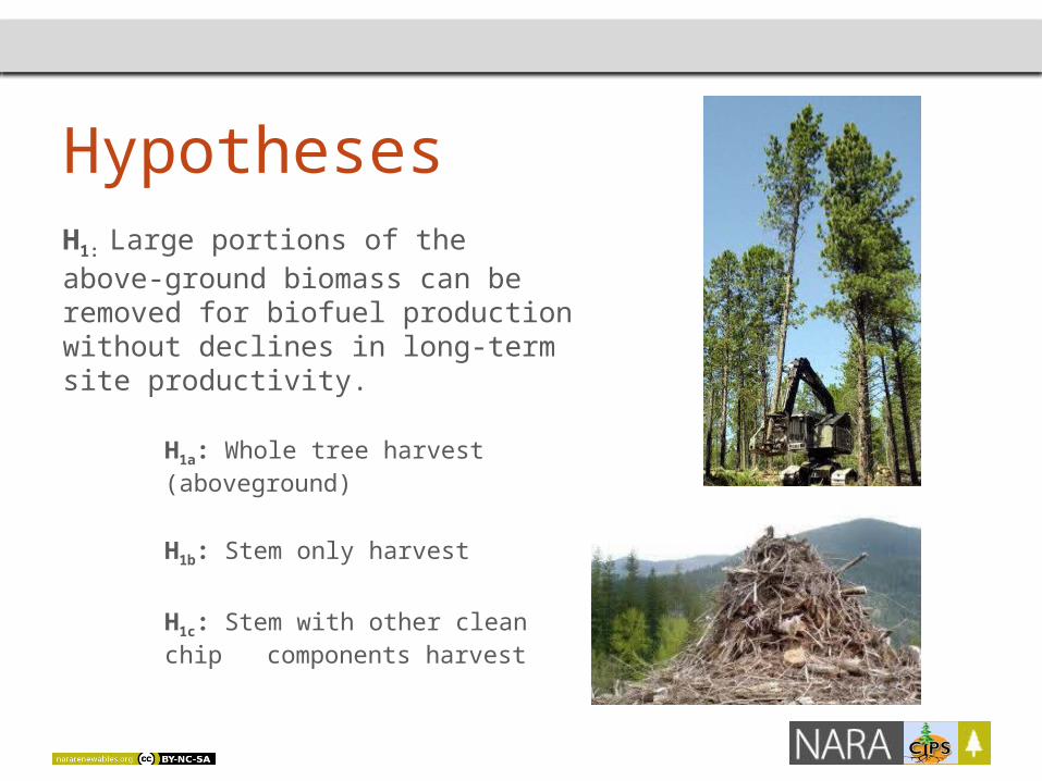
HypothesesH1: Large portions of the above-ground biomass can be removed for biofuel production without declines in long-term site productivity.

­ H1a: Whole tree harvest

(aboveground)

­ H1b: Stem only harvest

­ H1c: Stem with other clean chip

components harvest 

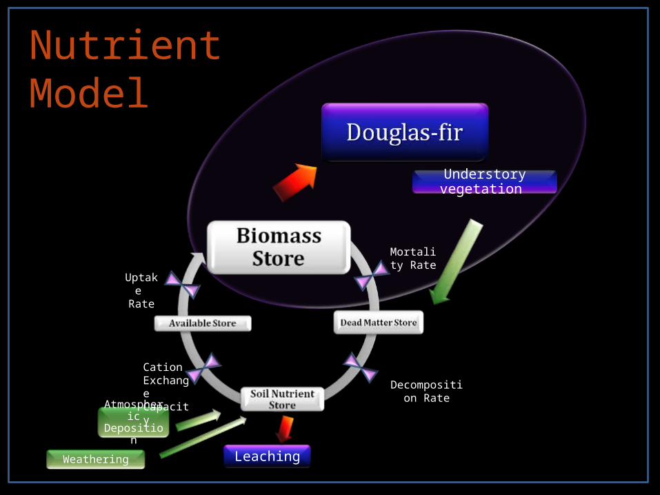
Leaching

Atmospheric Deposition

Uptake Rate

Mortality Rate

Decomposition Rate

Cation Exchange Capacity

Nutrient Model

Weathering

Understory vegetation

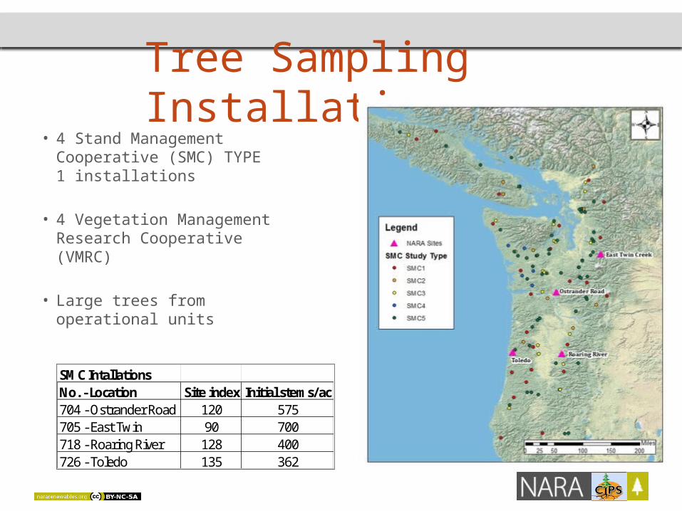
Tree Sampling Installations• 4 Stand Management

Cooperative (SMC) TYPE 1 installations

• 4 Vegetation Management Research Cooperative (VMRC)

• Large trees from operational units

SMC IntallationsNo. - Location Site index Initial stems/ac704 - Ostrander Road 120 575705 - East Twin 90 700718 - Roaring River 128 400726 - Toledo 135 362

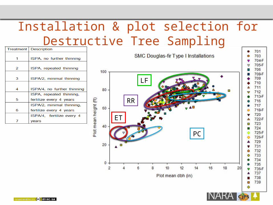
Installation & plot selection for Destructive Tree Sampling

PC

ET

RR

LF

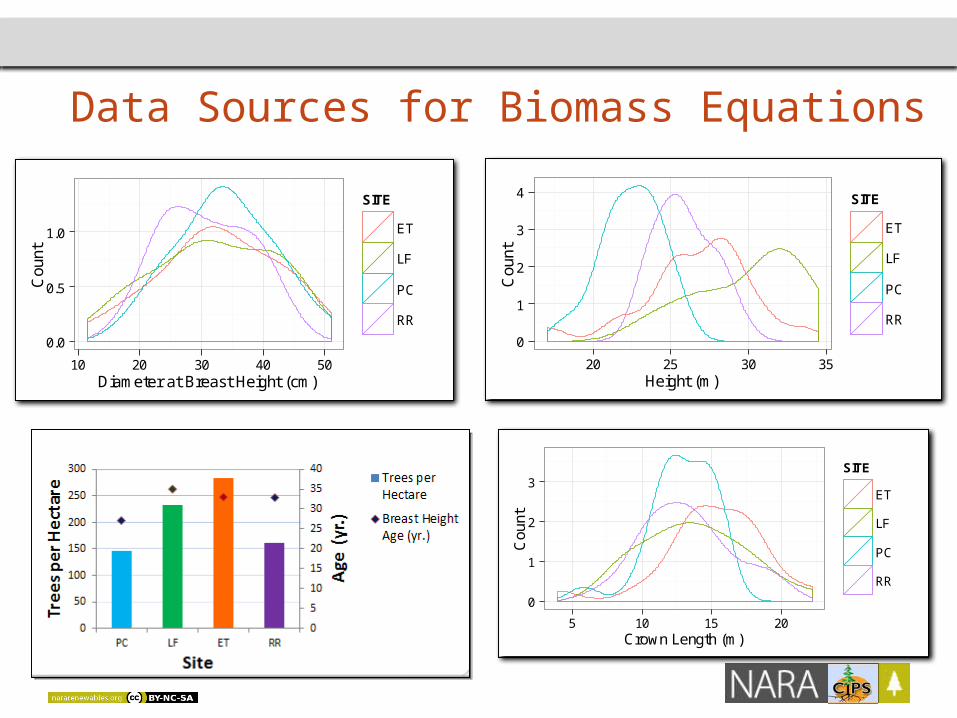
Data Sources for Biomass Equations

0

1

2

3

4

20 25 30 35Height (m)

Cou

nt

SITE

ET

LF

PC

RR

0

1

2

3

5 10 15 20Crown Length (m)

Cou

nt

SITE

ET

LF

PC

RR

0.0

0.5

1.0

10 20 30 40 50Diameter at Breast Height (cm)

Cou

nt

SITE

ET

LF

PC

RR

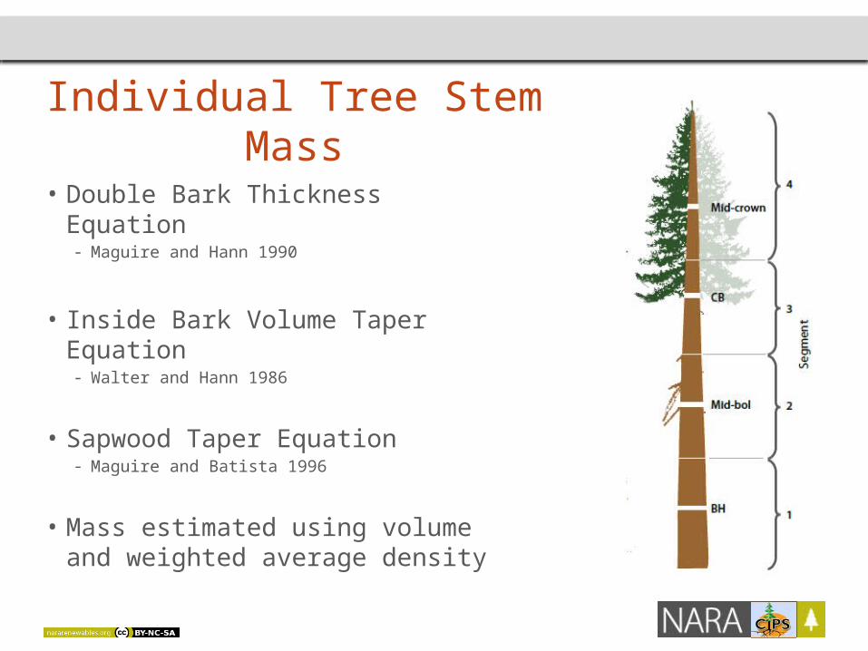
Individual Tree Stem Mass

• Double Bark Thickness Equation- Maguire and Hann 1990

• Inside Bark Volume Taper Equation - Walter and Hann 1986

• Sapwood Taper Equation- Maguire and Batista 1996

• Mass estimated using volume and weighted average density

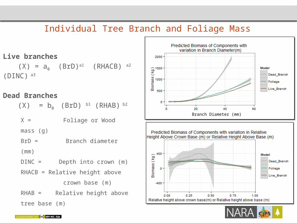
Individual Tree Branch and Foliage Mass

Live branches (X) = a0 (BrD)a1 (RHACB) a2 (DINC) a3

Dead Branches(X) = b0 (BrD) b1 (RHAB) b2

X = Foliage or Wood mass (g)

BrD = Branch diameter (mm)

DINC = Depth into crown (m)

RHACB = Relative height above

crown base (m)

RHAB = Relative height above tree base (m)

Branch Diameter (mm)

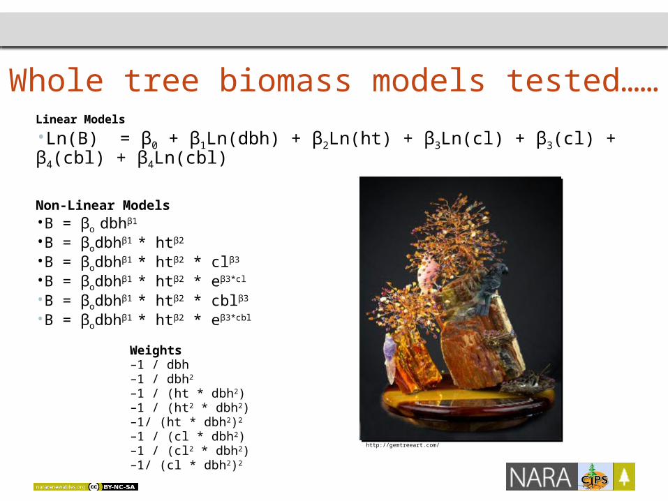
Whole tree biomass models tested……Linear Models

•Ln(B) = β0 + β1Ln(dbh) + β2Ln(ht) + β3Ln(cl) + β3(cl) + β4(cbl) + β4Ln(cbl) 

Non-Linear Models•B = βo dbh 1β

•B = βodbh 1 β * ht 2β

•B = βodbh 1 β * ht 2β * cl 3β

•B = βodbh 1 β * ht 2β * e 3*clβ

•B = βodbh 1 β * ht 2β * cbl 3β

•B = βodbh 1 β * ht 2β * e 3*cblβ

Weights –1 / dbh–1 / dbh2

–1 / (ht * dbh2)–1 / (ht2 * dbh2)–1/ (ht * dbh2)2

–1 / (cl * dbh2)–1 / (cl2 * dbh2)–1/ (cl * dbh2)2

http://gemtreeart.com/

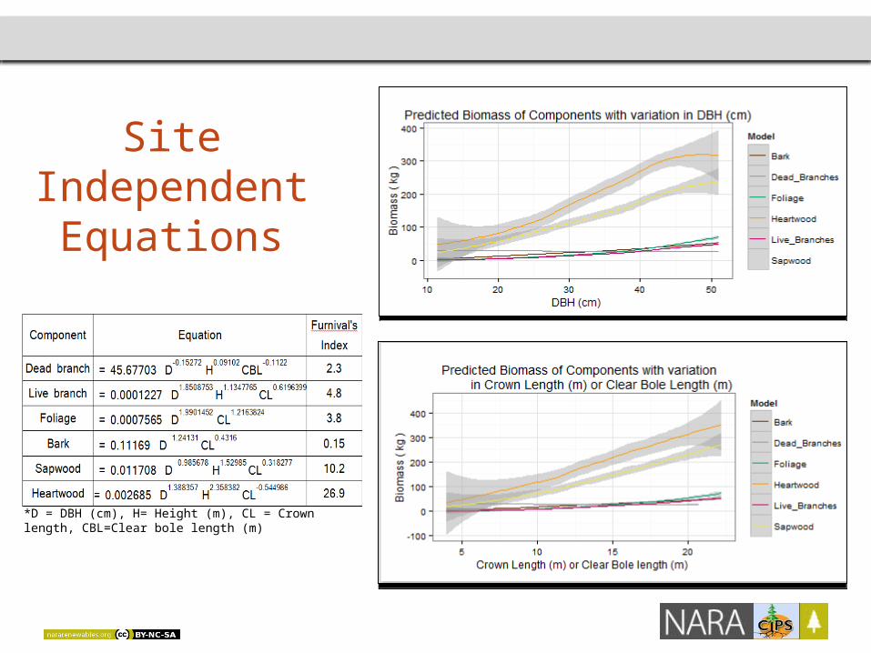
*D = DBH (cm), H= Height (m), CL = Crown length, CBL=Clear bole length (m)

Site Independent

Equations

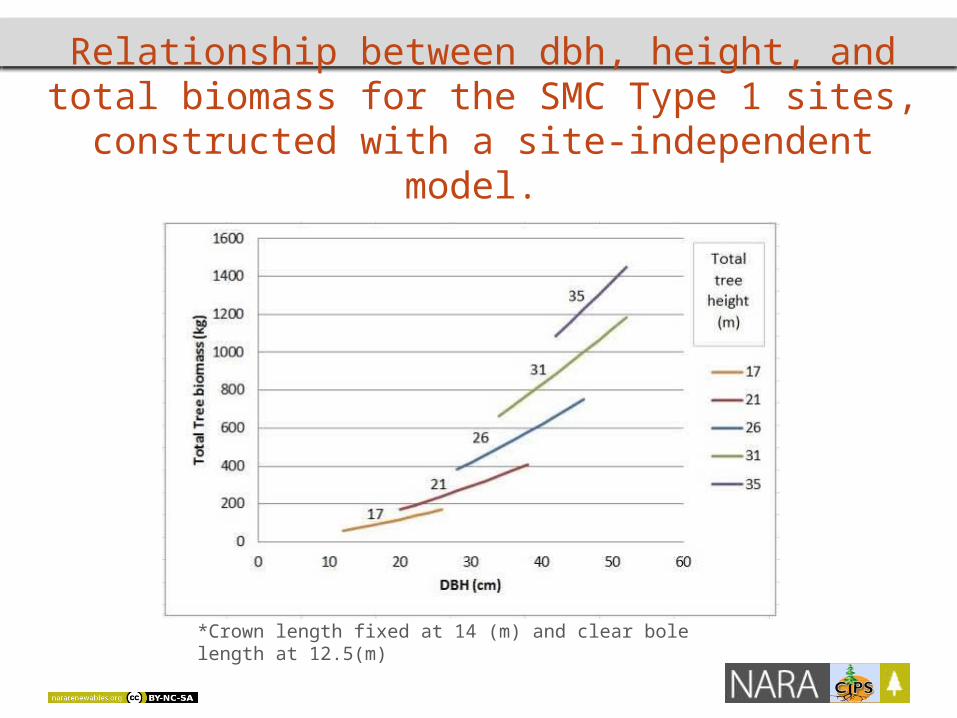
Relationship between dbh, height, and total biomass for the SMC Type 1 sites, constructed

with a site-independent model.

*Crown length fixed at 14 (m) and clear bole length at 12.5(m)

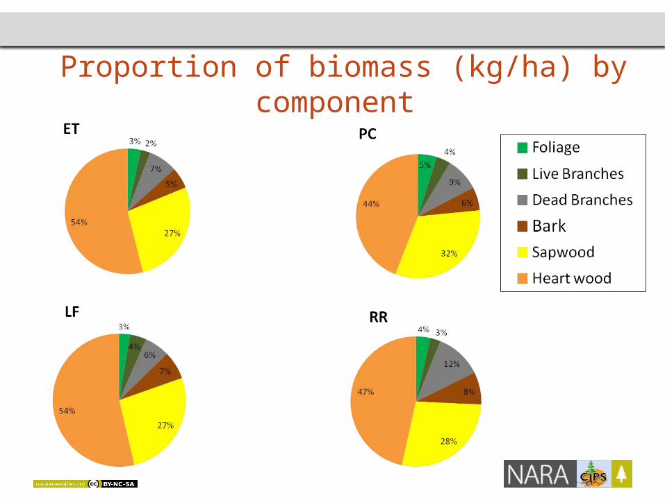
Proportion of biomass (kg/ha) by component

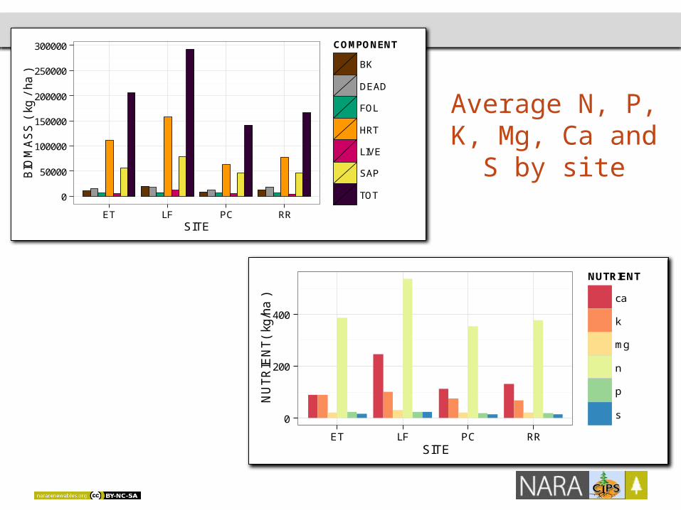
Average N, P, K, Mg, Ca and

S by site

0

200

400

ET LF PC RRSITE

NU

TR

IEN

T(

kg/h

a )

NUTRIENT

ca

k

mg

n

p

s

0

50000

100000

150000

200000

250000

300000

ET LF PC RRSITE

BIO

MA

SS

( k

g /

ha )

COMPONENT

BK

DEAD

FOL

HRT

LIVE

SAP

TOT

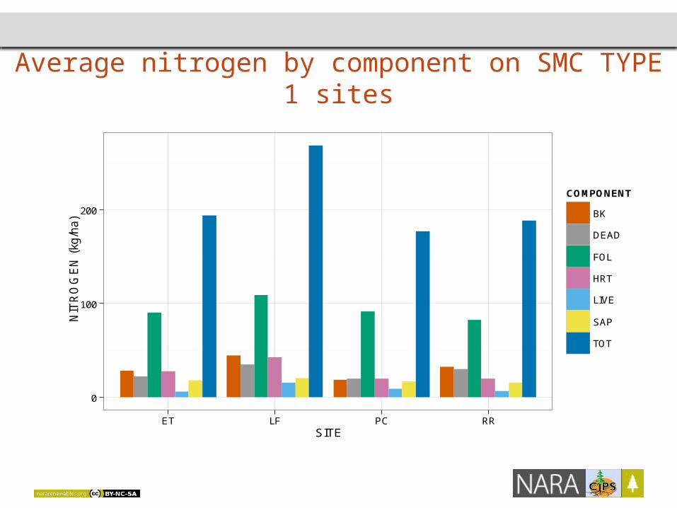
Average nitrogen by component on SMC TYPE 1 sites

0

100

200

ET LF PC RRSITE

NIT

RO

GE

N (

kg/h

a)

COMPONENT

BK

DEAD

FOL

HRT

LIVE

SAP

TOT

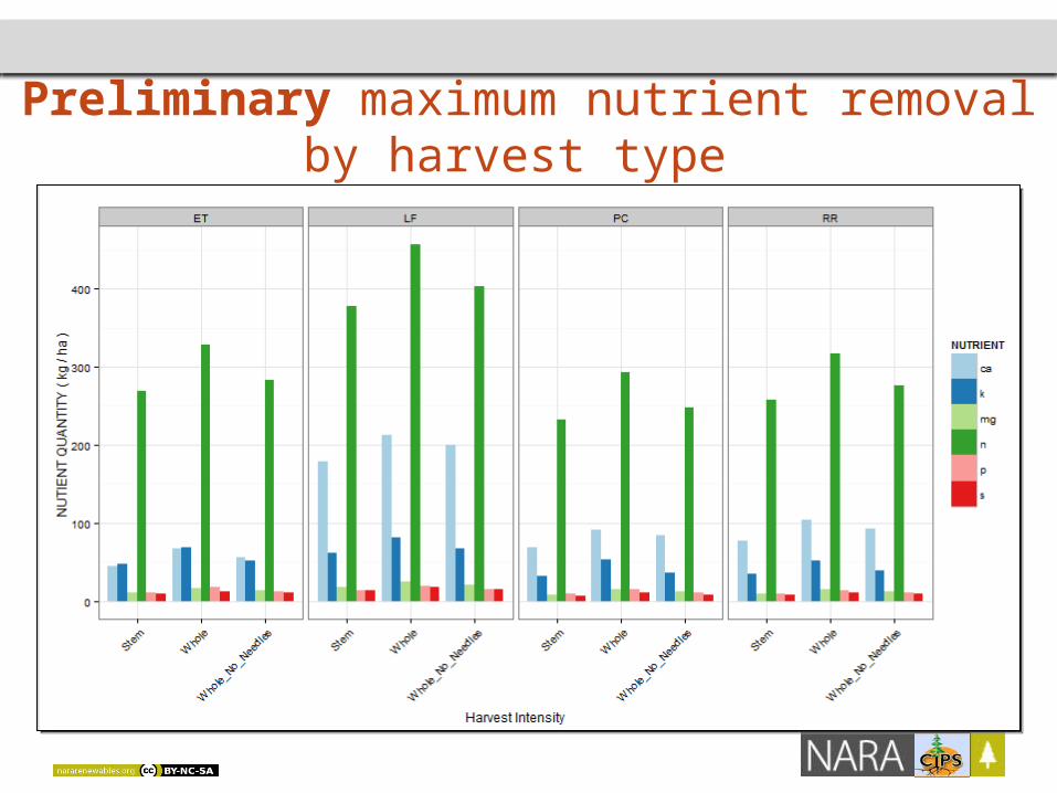
Preliminary maximum nutrient removal by harvest type

Any Questions or Comments?

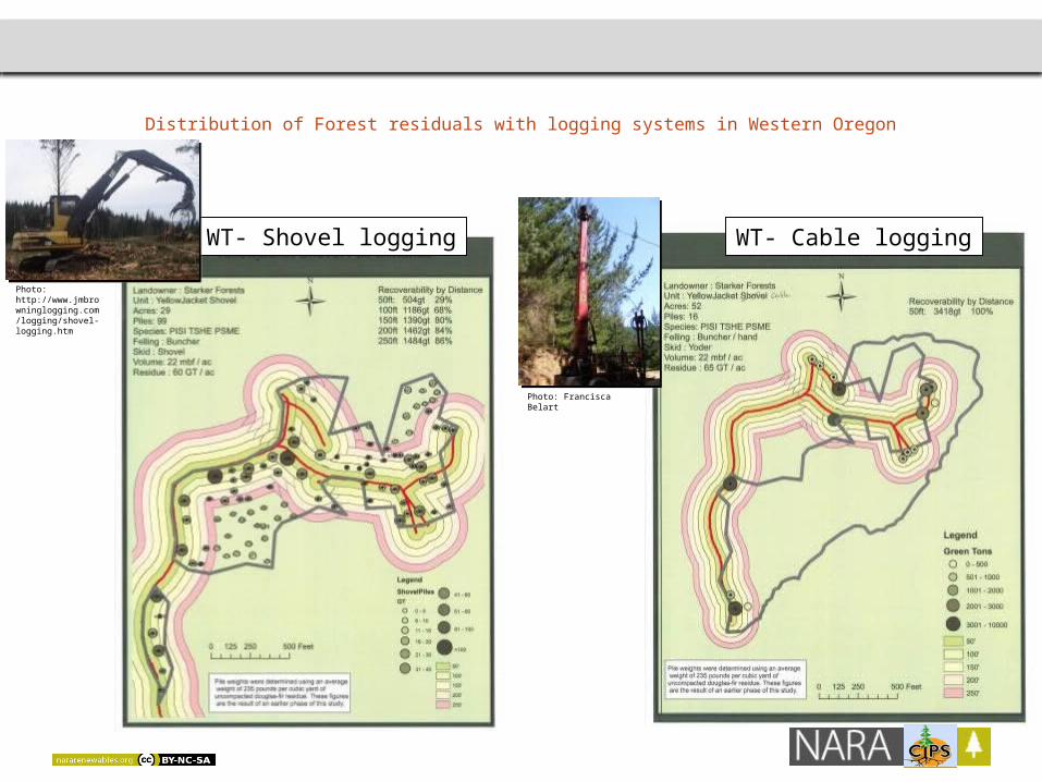
Distribution of Forest residuals with logging systems in Western Oregon

Photo: Francisca Belart

Photo: http://www.jmbrowninglogging.com/logging/shovel-logging.htm

WT- Cable loggingWT- Shovel logging

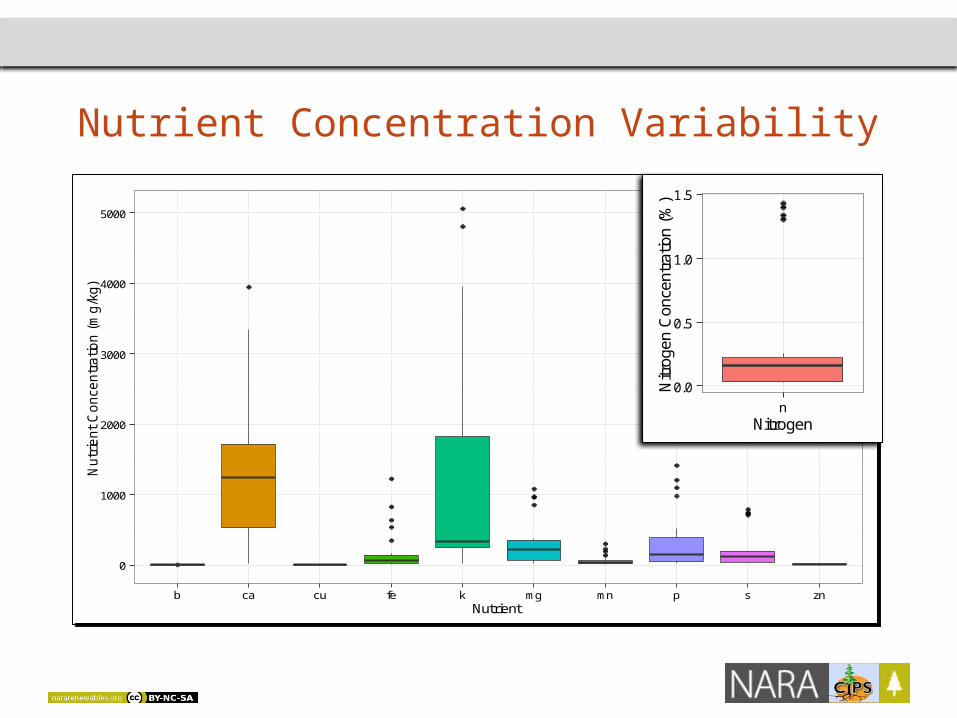
Nutrient Concentration Variability

0

1000

2000

3000

4000

5000

b ca cu fe k mg mn p s znNutrient

Nutr

ient

Conce

ntr

atio

n (

mg/k

g)

0

1000

2000

3000

4000

5000

b ca cu fe k mg mn p s znNutrient

Nutr

ient

Conce

ntr

atio

n (

mg/k

g)

0.0

0.5

1.0

1.5

nNitrogen

Nitr

ogen

Con

cent

ratio

n (%

)

Component biomass(%) averaged over treatment type

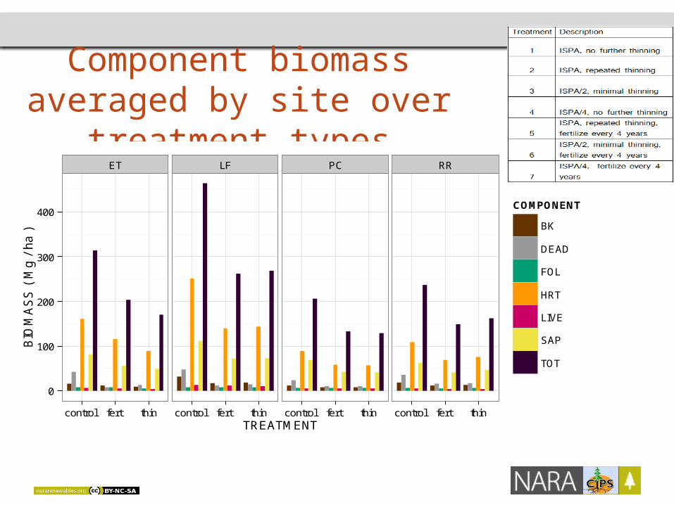
Component biomass averaged by site over

treatment types

presentation title

ET LF PC RR

0

100

200

300

400

control fert thin control fert thin control fert thin control fert thinTREATMENT

BIO

MA

SS

( M

g /

ha )

COMPONENT

BK

DEAD

FOL

HRT

LIVE

SAP

TOT

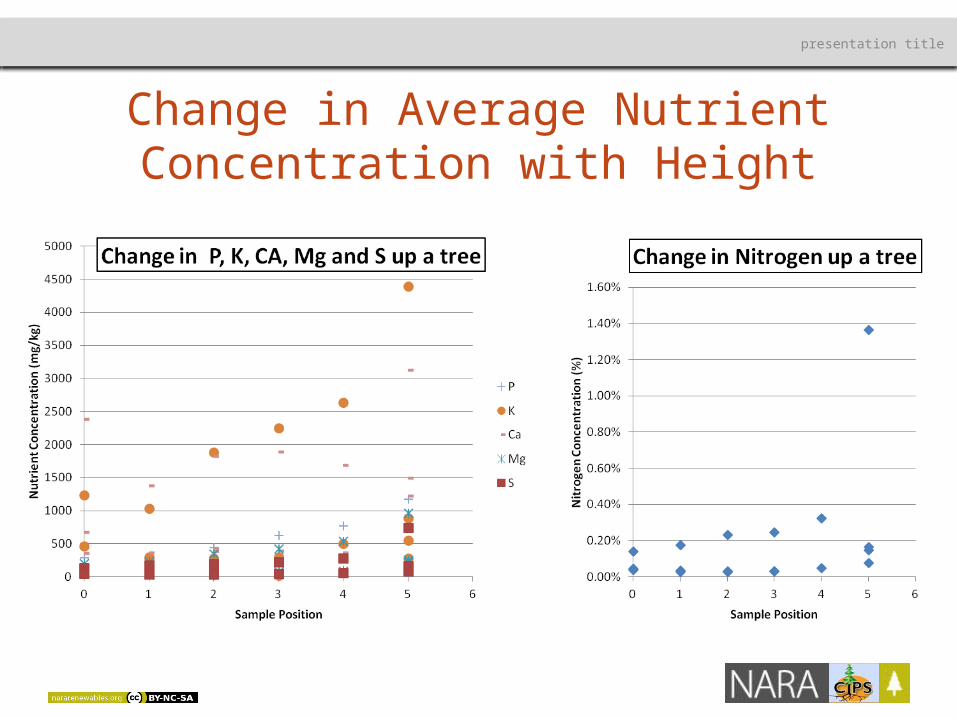
Change in Average Nutrient Concentration with Height

presentation title

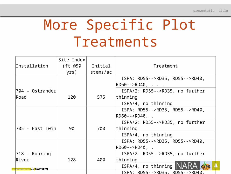
More Specific Plot Treatments

presentation title

Installation Site Index (ft @50 yrs) Initial stems/ac

Treatment

ISPA: RD55-->RD35, RD55-->RD40, RD60-->RD40, . . .704 – Ostrander Road 120 575 ISPA/2: RD55-->RD35, no further thinning ISPA/4, no thinning ISPA: RD55-->RD35, RD55-->RD40, RD60-->RD40, .705 - East Twin 90 700 ISPA/2: RD55-->RD35, no further thinning ISPA/4, no thinning ISPA: RD55-->RD35, RD55-->RD40, RD60-->RD40, .718 - Roaring River 128 400 ISPA/2: RD55-->RD35, no further thinning ISPA/4, no thinning ISPA: RD55-->RD35, RD55-->RD40, RD60-->RD40, .726 - Toledo 135 362 ISPA/2: RD55-->RD35, no further thinning ISPA/4, no thinning

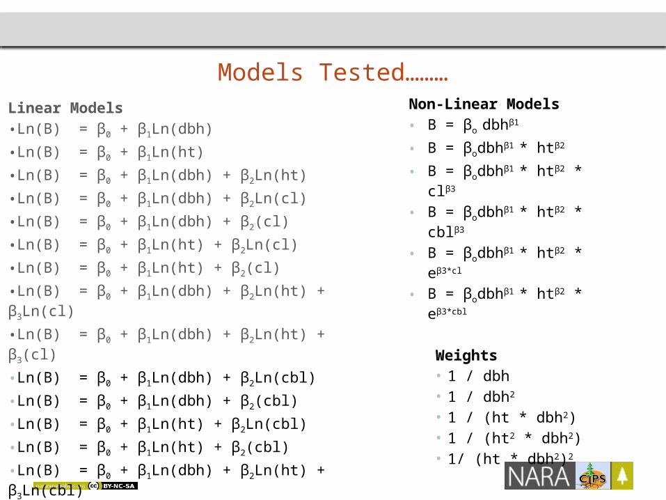
Models Tested………Linear Models•Ln(B) = β0 + β1Ln(dbh)

•Ln(B) = β0 + β1Ln(ht)

•Ln(B) = β0 + β1Ln(dbh) + β2Ln(ht)

•Ln(B) = β0 + β1Ln(dbh) + β2Ln(cl)

•Ln(B) = β0 + β1Ln(dbh) + β2(cl)

•Ln(B) = β0 + β1Ln(ht) + β2Ln(cl)

•Ln(B) = β0 + β1Ln(ht) + β2(cl)

•Ln(B) = β0 + β1Ln(dbh) + β2Ln(ht) + β3Ln(cl)

•Ln(B) = β0 + β1Ln(dbh) + β2Ln(ht) + β3(cl)

•Ln(B) = β0 + β1Ln(dbh) + β2Ln(cbl)

•Ln(B) = β0 + β1Ln(dbh) + β2(cbl)

•Ln(B) = β0 + β1Ln(ht) + β2Ln(cbl)

•Ln(B) = β0 + β1Ln(ht) + β2(cbl)

•Ln(B) = β0 + β1Ln(dbh) + β2Ln(ht) + β3Ln(cbl)

•Ln(B) = β0 + β1Ln(dbh) + β2Ln(ht) + β3(cbl)

 

Non-Linear Models• B = βo dbh 1β

• B = βodbh 1 β * ht 2β

• B = βodbh 1 β * ht 2β * cl 3β

• B = βodbh 1 β * ht 2β * cbl 3β

• B = βodbh 1 β * ht 2β * e 3*clβ

• B = βodbh 1 β * ht 2β * e 3*cblβ

Weights • 1 / dbh• 1 / dbh2

• 1 / (ht * dbh2)• 1 / (ht2 * dbh2)• 1/ (ht * dbh2)2