north- development and evaluation of five fuzzy...

NORTH- HOIJ-AND

Development and Evaluation of Five Fuzzy Multiattribute Decision-Making Methods Evangelos Triantaphyllou and Chi-Tun Lin

Department o f Industrial Engineering, Louis iana State University, Baton Rouge, Louis iana

ABSTRACT

We present the development o f five fuzzy multiattribute decision-making methods. These methods are based on the analytic hierarchy process (original and ideal mode), the weighted-sum model, the weighted-product model, and the TOPSlS method. More- over, these methods are examined in terms of two evaluative criteria. Computational results on test problems suggest that although all the methods are inaccurate, some of them seem to be more accurate than the others. The proposed evaluation methodology can easily be used in evaluating more fuzzy multiattribute decision making methods.

KEYWORDS: Fuzzy decision-making, multiattribute decision.making, ranking of fuzzy numbers, pairwise comparisons, analytic hierarchy process, weighted-sum model, weighted-product model, TOPSlS method.

1. BACKGROUND INFORMATION

One of the most crucial problems in many decision-making methods is the precise evaluation of the pertinent data. Very often in real-life decision-making applications data are imprecise and fuzzy (see, for instance, [32], [21, [34], [4], [24, 261, and [15]). For example, how can one quantify statements such as "What is the value of the j th alternative in terms of an environmental impact criterion?" A decision maker may encounter difficulty in quantifying and processing such linguistic statements. Therefore, it is desirable to develop decision-making methods

Address correspondence to Evangelos Triantaphyllou, Department of Industrial Engineering, 3128 CEBA Building, Louisiana State University, Baton Rouge, LA 70803-6409. E-mail: ietrian @lsuvm.sncc.lsu.edu.

Received January 1995; accepted September 1995.

International Journal of Approximate Reasoning 1996; 14:281-310 © 1996 Elsevier Science Inc. 0888-613X/96/$15.00 655 Avenue of the Americas, New York, NY 10010 SSDI 0888-613X(95)00119-0

282 Evangelos Triantaphyllou and Chi-Tun Lin

which use fuzzy data. It is equally important to evaluate the performance of these fuzzy decision-making methods.

In [6], [8], and [16] a fuzzy version of Saaty's [20] AHP method was developed. In that version of fuzzy AHP, triangular fuzzy numbers were used with pairwise comparisons in order to compute the weights of importance of the decision criteria. Also, the fuzzy performance values of the alternatives in terms of each decision criterion were computed by using triangular fuzzy numbers. The fuzzy operations which were used by these authors are also applied later in this paper to fuzzify four more crisp decision-making methods. These five methods are the weighted-sum model (WSM), the weighted-product model (WPM), the revised AHP (RAHP) (as proposed by Belton and Gear [3]; it is also known as the ideal model AHP [21]), and the TOPSlS method [13]. These methods are briefly described in the next section.

2. SOME CRISP DECISION-MAKING METHODS

2.1. The Weighted-Sum Model

The WSM is probably the best-known and most widely used method of decision making. Suppose that there are M alternatives and N criteria in a decision-making problem. Then the best alternative, A*, is the one which satisfies (in the maximization case) the following expression [12, 11]:

N

* = ~ aijWj, (2-1) PWS M max M>_i>_l i - I

where PWSM is the WSM priority score of the best alternative, aij is the measure of performance of the ith alternative in terms of the j th decision criterion, and wj is the weight of importance of the j th criterion.

The WSM method can be applied without difficulty in single-dimensional cases where all units of measurement are identical (for example, dollars, milage, hours, etc.). Because of the additivity utility assumption, a conceptual violation occurs when the WSM is used to solve multidimensional problems in which the units are different.

2.2. The Weighted-Product Model

The WPM uses multiplication to rank alternatives. Each alternative is compared with others by multiplying a number of ratios, one for each criterion. Each ratio is raised to the power of the relative weight of the

Five Multiattribute DM Methods 283

corresponding criterion. Generally, in order to compare the two alternatives A K and A L, the following formula is used [7, 19, 11]: ()6()w

A K aK__L

R ~ L = j= 1 aLj ' (2-2)

If the above ratio is greater than or equal to one, then (in the maximization case) the conclusion is that alternative A K is bet ter than alternative A L. Obviously, the best alternative A* is the one which is bet ter than or at least as good as all other alternatives.

Note that the WPM is very similar to the WSM. The WPM is sometimes called dimensionless analysis because its structure eliminates any units of measure. Thus, the WPM can be used in single- and multidimensional decision problems. Also, the relative values of the measure of the ith alternative in terms of the j th criterion can be replaced with actual values in this method.

2.3. The Analytic Hierarchy Process

The final step of the A H P approach deals with the construction of an M × N matrix (where M is the number of alternatives and N is the number of criteria). In this matrix the element aij represents the relative performance of the ith alternative in terms of the j th criterion. The vector X i = ( a i d a i 2 , . . . , a i N ) for the ith alternative (i = 1,2,-.., M) is the eigenvector of an N × N reciprocal matrix which is determined through a sequence of pairwise comparisons [20]. Also, the elements in each such vector add up to one. The A H P uses relative values instead of actual ones. Therefore, the A H P can be used in single- and multidimensional decision- making problems. The formula used by the A H P (or the RAHP) is the same as the one used by the WSM [i.e., Equation (2-1)].

2.4. The Revised Analytic Hierarchy Process

The RAHP, which was proposed by Belton and Gear [3], is a revised version of the original A H P model. They observed that sometimes it is possible for the A H P to yield unjustifiable ranking reversals. In [3] a numerical example is demonstra ted which consists of three alternatives and three criteria. Next, a new alternative, identical to a nonoptimal alternative, is introduced. As result, the ranking of the existing alternatives changes.

The reason for that ranking inconsistency, according to Belton and Gear, is that the relative performance measures of all alternatives in terms of each criterion summed to one. Instead of having the relative values sum


to one, they propose to divide each relative value by the maximum value in the corresponding vector of relative values. Later, Saaty [21] accepted this variant of the original AHP, and now it is also known as the ideal-mode AHP.

2.5. The TOPSIS Method

TOPSIS (the Technique for Order Preference by Similarity to Ideal Solution) was developed by Hwang and Yoon [13] as an alternative to the ELZCTRE method [5]. The basic concept of this method is that the selected best alternative should have the shortest distance from the ideal solution and the farthest distance from the negative-ideal solution in a geometrical (i.e., Euclidean) sense.

TOPSlS assumes that each attribute has a tendency toward monotonically increasing or decreasing utility. Therefore, it is easy to locate the ideal and negative-ideal solutions. The Euclidean distance is used to evaluate the relative closeness of alternatives to the ideal solution. Thus, the preference order of alternatives is derived by comparing these relative distances.

The TOPSIS method evaluates the following decision matrix, which refers to m alternatives which are evaluated in terms of n criteria:

Criterion

C 1 C 2 C 3 "" C,, Alt. W 1 W 2 W 3 "'" W n

A1 Xll x12 x13 . . . Xln

A2 x21 x22 x23 • .. X2n

A3 x31 x32 x33 •. . X3n

A m Xml Xm2 Xm3 "'" Xmn

where A i is the ith alternative, Cj is the j th criterion, and xij is the performance measure of the ith alternative in terms of the j th criterion. Then the TOPSIS method consists of the following steps (which are adapta- tions of the corresponding steps of the ELECTRE method).

Step 1: Construct the normalized decision matrix. This step converts the various attribute dimensions into nondimensional attributes, as in the ELECTRE method. An element rij of the normalized decision matrix R is calculated as follows:

xij (2-3) rij ~ m l X 2


Step 2: Construct the weighted normalized de~ision matrix. A set of weights W = (w 1, w 2, ... w n) (such that Ew i = 1), specified by the decision maker , is used in conjunct ion with the previous normal ized decision matr ix to de t e rmine the weighted normal ized matr ix V defined as V = (rijWj).

Step 3: Determine the ideal and the negative-ideal solutions. T h e ideal (A*) and the negat ive- ideal ( A - ) solutions are def ined as follows:

or/= m)

= {v~', v~, v 3 , " ' , v, }, (2-4)

= { V l , U 2 , U 3 , ' " , Un} , ( 2 - 5 )

where

J = {j -- 1 ,2 , - - - n I j associated with the benef i t criteria}

and

J ' = {j = 1 ,2 , - . - n L j associa ted with the cost criteria}.

For benefi t criteria, the decision m a k e r desires to have a m a x i m u m value a m o n g the alternatives. Fo r cost criteria, however , the decision m a k e r desires to have a m i n i m u m value among them. Obviously, A* indicates the mos t p re fe rab le a l ternat ive or ideal solution. Similarly, A - indicates the least p re fe rab le a l ternat ive or negat ive- ideal solution.

Step 4: Calculate the separation measure. In this step the concept of the n-d imens iona l Eucl idean distance is used to measu re the separa t ion distances of each a l ternat ive to the ideal solut ion and negat ive- ideal solution. The cor responding fo rmulas are

S i . = V [ ~ (Uij -- V j , )2 for i = 1, 2, 3,---, m , (2-6)

where S i . is the separa t ion (in the Eucl idean sense) of a l ternat ive i f rom the ideal solution, and

S i = ~/ ~ (Vij -- Vj_ )2 for i = 1 ,2 , 3 , - " , m , (2-7)


where S i is the separation (in the Euclidean sense) of alternative i from the negative-ideal solution.

Step 5: Calculate the relative closeness to the ideal solution. Next, the relative closeness of alternative Ai with respect to the ideal solution A* is defined as follows:

S i _ Ci , 0 < C i , <_ 1, i = 1 ,2 , - ' . ,m . (2-8)

S i , -~- S i

E v i d e n t l y , C i , = ] if and only if A i = A*, and C i _ : 0 if and only if A i = A - .

Step 6: Rank the preference order. The best satisfied alternative can now be decided according to preference rank order of C i , . It is the one which has the shortest distance to the ideal solution. The way the alternatives are processed in the previous steps reveals that if an alternative has the shortest distance to the ideal solution, then this alternative is guaranteed to have the longest distance to the negative-ideal solution.

3. OPERATIONS ON FUZZY TRIANGULAR NUMBERS

Most of the decision making in the real world takes place in a situation in which the pertinent data and the sequences of possible actions are not precisely known. Therefore, it is very important to adopt fuzzy data to express such situations in decision-making problems. In order to fuzzify the previous five crisp decision-making methods, it is important to know how fuzzy operations are used on fuzzy numbers. Fuzzy operations were first introduced by Dubois and Prade [10, 9]. Other researchers, such as Laarhoven and Pedrycz [16], Buckley [8], and Boender et al. [6], treated a fuzzy version of the AHP by using the fuzzy operations introduced by Dubois and Prade.

When the decision maker considers the problem of ranking the M alternatives A s, A2,-.., A M with respect to the N criteria C~, C2,..., CN, he or she will feel great difficulty in assigning numbers, or ratios of numbers to alternatives in terms of these criteria. The merit of using a fuzzy approach is to assign the relative importance of attributes using fuzzy numbers instead of crisp numbers. For fuzzy numbers we use triangular fuzzy numbers (that is, fuzzy numbers with lower, modal, and upper values), because they are simpler than trapezoidal fuzzy numbers. A fuzzy triangular number is defined as follows:


DEFINITION [9] A fuzzy number M on R ~ ( - oo, + be) is defined to be a fuzzy triangular number if its membership function ]£m : g ~ [0, 1] i s equal to

/+:m/ m,(x) = l (3-1)

, x ~ [ m , u ] ,

~ o - U m - u otherwise,

where l _< m _< u, and l and u stand for the lower and upper values of the support of the fuzzy number M, respectively, and m for the modal value. A fuzzy triangular number, as expressed by Equation (3-1), will be denoted by (l, m, u).

Laarhoven and Pedrycz [16], Buckley [8], and Boender et al. [6] introduced fuzzy number operations in Saaty's AHP method by replacing crisp numbers with triangular fuzzy numbers. The distinction of Buckley's method from Boender's is that the fuzzy solution of a decision-making problem does not need to be approximated by fuzzy triangular numbers. However, the triangular approximation of fuzzy operations is plausible for fuzzifying the implicit solution of a decision-making problem and provides fuzzy solutions with much smaller spread than Buckley's method [6]. Also, Boender et al. proposed the use of a geometric ratio scale as opposed the original Saaty equidistant scale in quantifying the gradations of a human's comparative judgements. The basic operations on fuzzy triangular numbers which were developed and used in [16] are defined as follows:

711 ~ n2 = (nat + n2l, nlm + n2m, nlu + n2u) for addition,

/~1 ~ fi2 = (rill >( n21, him X n2rn, nlu x nzu ) for multiplication,

Off1 = (-nmu, -n~m, - n i t ) for negation,

1/fi I --- (1/nlu, 1/n lm, 1~nit) for division,

ln(fi l) --- (In(nit), ln(nim), ln(nl~)) for natural logarithm,

exp(fi 1) =- (exp(nlt), exp(nlm), exp(nlu)) for exponential,

where -- denotes approximation, and f i l - - (n l l , nlm, nlu) and fi2 = (n2l , n2m , n2u) represent two fuzzy triangular numbers with lower, modal, and upper values. For the special case of raising a fuzzy triangular number of the power of another fuzzy triangular number, the following approximation was used:

n 1 tl2m n2u fi~2 -_ (nl{ ,nl m ,nl ~ ).


Note that this formula was used only in the development of the fuzzy WPM (as explained later).

4. RANKING OF FUZZY NUMBERS

The problem of ranking fuzzy numbers appears very often in the literature. For instance, a comparison and evaluation of different ranking approaches is described in [18] and [33]. As each method of ranking fuzzy numbers has its advantages over the others in certain situations, it is very difficult to determine which method is the best one. Some important factors in deciding which ranking method is the most appropriate for a given situation include the complexity of the algorithm, its flexibility, accuracy, ease of interpretation, and the shape of the fuzzy numbers which are used.

A widely accepted method for comparing fuzzy numbers was first introduced by Baas and Kwakernaak [1]. Tong and Bonissone [22] introduced the concept of a dominance measure and proved it to be equivalent to Baas and Kwakernaak's ranking measure. This method was also later adopted by Buckley [8]. According to Zhu and Lee [33] this ranking method is less complex and still effective. It allows a decision maker to implement it without difficulty and with ease of interpretation. Therefore, in this paper we use this method in ranking fuzzy triangular numbers. However, a given problem may require a different method.

The above procedure for ranking triangular fuzzy numbers is used as follows. Let /~i(x) denote the membership function for the fuzzy number fi i. Next, define

max min( /~i (x) , /~ j (y))} for all i, j = 1,2, 3,-.., m. (4-1) CiJ ~" x>y_ {

Then /2i dominates (or outranks) fij, written as fii > fij, if and only if eij = 1 and eji < Q, where Q is some fixed positive fraction less than one. Values such as 0.7, 0.8, or 0.9 might be appropriate for Q; the value should be set by the analyst and possibly be varied for a sensitivity analysis. In the computational experiments reported later in this study the value Q = 0.9 was used. The above concepts are best explained in the following illustrative example:

EXAMPLE 4-1 Suppose that the importances of two alternatives A 1 and A 2 are represented by the two fuzzy triangular numbers fil = (0.2, 0.4, 0.6) and fi2 = (0.4,0.7,0.9), respectively. Next, observe from Figure l that e21 = 1 and e12 = 0 . 4 < Q = 0.9. Therefore, the best alternative is A 1.


/.£m

51 ~2 l . 00 . . . . . . . . . . . . . . . . . . . . . . . . . . . . . . . . . . . . . . .

#,( n=

elo = 0.40

0.00 g . 8 0 0 . 2 8 0 . 4 0 0 . 6 0 0 . B 0 J . . ~

X

Figure 1. Membership functions for the fuzzy alternatives A 1 and A 2.

5. FUZZIFICATION OF THE CRISP MADM METHODS

In the following subsections the procedures applied by Laarhoven and Pedrycz [16] and Boender et al. [6] will be used on the crisp multiattribute decision methods (MADM) described in Section 2. Some numerical examples are also given for a better illustration of these procedures.

5.1. The Fuzzy Weighted-Sum Model

Recall that the best alternative according to this model is the one which satisfies Equation (2-1). Now, the performance value of the ith alternative in terms of the j th criterion is a fuzzy triangular number denoted as aij = (aijl, aijm, aiju). Analogously, it is assumed that the decision maker will use fuzzy triangular numbers in order to express the weights of importance of the criteria. These weights are denoted as ~j = (Wyl, Wjm , Wju). Also, to be consistent with the basic requirement that the weights usually add up to one (in a crisp environment), now it is required that the sum of Wjm (the modal values of the fuzzy triangular numbers which represent the criterion weights) be equal to one. From the above considerations it follows that now the best alternative is the one which satisfies the following relation:

N

PFWSM : max ~ aijWj f o r i = 1 , 2 , 3 , ' " , M. (5-1) j = l


EXAMPLE 5-1 Let a decision problem be defined on the four criteria CI, C 2, C 3, C a and the three alternatives A1, A z, A 3. Suppose that the data for this problem are as shown in the following fuzzy decision matrix:

C 1 C 2 C3 Ca (0.13,0.20,0.31) (0.08,0.15,0.25) (0.29,0.40,0.56) (0.17,0.25,0.38)

~zl 1

A2 A3

(3.00, 4.00, 5.00) (6.00, 7.00, 8.00) (4.00, 5.00, 6.00)

(5.00, 6.00, 7.00) (5.00, 6.00, 7.00) (5.00, 6.00, 7.00) (0.50, 1.00, 2.00) (3.00, 4.00, 5.00) (7.00, 8.00, 9.00)

(2.00, 3.00, 4.00) (4.00, 5.00, 6.00) (6.00, 7.00, 8.00)

Therefore, when the fuzzy WSM approach is used, the final priority scores (denoted as P1, P2, and P3) of the alternatives are

P1 = (0.13,0.20,0.31) × (3.00,4.00,5.00) + (0.08,0.15,0.25)

× (5.00, 6.00, 7.00) + (0.29, 0.40, 0.56) × (5.00, 6.00, 7.00) + (0.17, 0.25, 0.38) × (2.00, 3.00, 4.00)

= (2.583, 4.850, 8.750), and similarly,

P2 = (1.979~ 3.950, 7.625),

P3 = (3.792, 6.550, 11.188).

Figure 2 displays the membership functions of these final results. They could be interpreted as a measure of the ability of each alternative to meet

1 . 0 0 . . . . . . . . . . . . . . . . . .

Q = 0 . 9 0 . . . . . . . . . . . . . . . . . . . . . . . . . . . . . . . . . . / . . . . . . . . . . . . . . . . . .

d

0 . 0 0

3 .0 2 . 0 4 . 0 6 . 0 g . g 1 0 . 0 1 2 . 0

X Figure 2. Membership functions of the alternatives A1, A 2, and A 3 of Example 5-1 according to the fuzzy WSM.


the decision criteria. From this figure it is clear that e31 = e32 = el2 = 1, and e13, e23 , and e21 are less than Q (= 0.9). Thus, according to the ranking procedure which was discussed in Section 4, alternative A 3 is the most preferred alternative.

5.2. The Fuzzy Weighted-Product Model

The best alternative according to this model is the one which satisfies Equation (2-2). For the fuzzy version of this model the corresponding formula is

A K aKj R ~- ,

j = l aLj (5-2)

where aKj, aLj, and ffj are fuzzy triangular numbers. Alternative A K

dominates alternative A t if and only if the numerator in Equation (5-2) is greater than the denominator. The application of (5-2) is also illustrated in the following example:

EXAMPLE 5-2 The data used in Example 5-1 are also used here. When the relation (5-2) is used, the following ratios are obtained:

R(A1/A 2) = [(3.00, 4.00, 5.00) (0"13'0'20'0"31) X (5.00, 6.00, 7.00)(0-08,0.t5,0 -25)

X (5.00, 6.00, 7.00) (0"29'0"40'0"56) X (2.00, 3.00, 4.00) (0"17'0"25'0"38)

/ ( 6 . 0 0 , 7.00, 8.00) (°'13'0"2°'°'31) X (5.00, 6.00, 7.00) (°'°8'°'15'°'25)

x (0.50, 1.00, 2.00) (0"29'0"40'0"56) x (4.00, 5.00, 6.00) (0"17'0'25 ,0.38)]

= (2.355, 4.652, 13.516)/(1.473, 2.887, 9.008),

and similarly,

R(A1/A 3) = (2.355,4.652, 13.516)/(3.099, 6.348, 19.649),

R(Az /A 3) = (1.473, 2.887, 9.008)/(3.099, 6.348, 19.649).

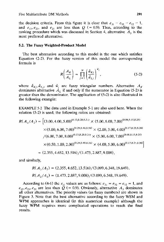
According to (4-1) the eq values are as follows: e31 = e32 = e12 = 1, and e13 , e23 , e21 are less than Q (= 0.9). Obviously, alternative A 3 dominates all other alternatives. The priority values (as fuzzy numbers) are shown in Figure 3. Note that the best alternative according to the fuzzy WSM and WPM approaches is identical (in this numerical example) although the fuzzy WPM requires more complicated operations to reach the final results.


1. oe

~.0 a.i

A t A 3

) 5.a 7 .e

X Figure 3. Membership functions of alternatives A1, A2, and A3 of Example 5-2 according to the fuzzy WPM.

5.3 The Fuzzy Analytic Hierarchy Process

In [16] and [6] a fuzzy version of the AHP method was presented. An example is shown below to illustrate that approach by using fuzzy triangular numbers.

EXAMPLE 5-3 Consider a decision problem with four criteria and three alternatives. Suppose that when the decision maker is asked to compare the three alternatives in terms of the first criterion by using pairwise comparisons, the following reciprocal judgment matrix was derived:

A 1

A2 A 3

A 1 A 2 A 3

(1,1,1) (~, ½, 2) (~-, 1 4-, 1 2 .~) (½, 2, 6) (1, 1, 1) (½, ~, 1) (3, 4, 10) (1, 3, 8) (1, 1, 1)

Note that when an alternative is compared with itself, the fuzzy number (1, 1, 1) is used instead of the crisp number 1.00.

Next, the fuzzy eigenvector of the above matrix is estimated. Recall that given a crisp reciprocal matrix, then according to Saaty the right principal eigenvector of the matrix expresses the importances of the alternatives. Some alternative procedures for estimating importances from pairwise


comparisons are discussed by Triantaphyllou et al. in [24, 26], and a partitioning method is presented by Triantaphyllou in [30]. Saaty [21] approximates the eigenvector by multiplying the elements in each row and then taking the nth root (an evaluation of that procedure can be found in [25, 28]). Therefore, the fuzzy version of the above procedure yields the following fuzzy importances of the three alternatives:

1 1/3 U 1 ~-~ [(1, 1, 1) × (-~, ½,2) x ( ~ , %, 2)]

1 v2 [(5,2, 6/ × (1, 1, 1) x (½, ½, 1)] 1/3

3 U3 [ ( 5 ' 4, 10) X (1,3,8) X (1,1, 1)] 1/3

= (0.25, 0.50, 1.10),

= (0.40, 0.87, 1.82),

= (1.14, 2.29, 4.31).

Next, the above vector is normalized according to the corresponding requirement in the original crisp AHP. The normalized vector is derived by dividing each entry by the sum of the entries in the vector. It can be easily verified that the normalized priority vector is

(0.02, 0.14, 0.99) ] (0.06, 0.24, 1.02)/. (0.16, 0.62, 2.41) J

At this point let us assume that the fuzzy eigenvectors of the pairwise comparisons when the three alternatives are compared in terms of each of the remaining criteria are also derived in a similar manner, along with the weights of importance of the four criteria, and form the vectors in the following fuzzy decision matrix:

C 1 C 2 C 3 C 4

(0.08,0.18,0.46) (0.08,0.16,0.39) (0.17,0.40,0.86) (0.11,0.26,0.61)

A 1

A2 A3

(0.02, 0.14, 0.99) (0.06, 0.24, 1.02) (0.16, 0.62, 2.41)

(0.18,0.44,0.95) (0.22,0.37,0.64) (0.12,0.23,0.55) (0.14,0.35,0.83) (0.07,0.10,0.15) (0.13,0.30,0.69) (0.11,0.21,0.53) (0.30,0.53,0.91) (0.19,0.47,1.00)

According to Equation (5-1) the final priority scores (denoted as P1, P2, and P3 ) of the three alternatives are as follows:

P1 = (0.02, 0.14, 0.99) x (0.08, 0.18, 0.46)

+ (0.18, 0.44, 0.95) x (0.08, 0.16, 0.39)

+ (0.22, 0.37, 0.64) x (0.17, 0.40, 0.86)

+(0.12,0.23,0.55) x (0.11,0.26,0.61)

= (0.068, 0.474, 1.887),


and similarly,

P2 = (0.772, 0.208, 1.908),

P3 = (0.897, 0.480, 2.696).

When the ranking procedure described in Section 4 is applied on P~, P2, and /'3, it can be easily shown that alternative A 3 is the best one.

Finally, it should be stated here that other pairwise comparison procedures require the comparisons not to be considered as ratios but as differences (see, for instance, [27]). A survey of some critical issues in the use of pairwise comparisons is presented in [29].

5.4. The Revised Analytic Hierarchy Process

As mentioned in Section 2.4., the revised version of the AHP (which is also called the ideal-modeAHP [21]) as proposed by Belton and Gear [3] is to normalize the relative performance measures of the alternatives in terms of each criterion by dividing the values by the largest one. This is the only difference from the original AHP method. The fuzzy version of the revised AHP is best illustrated in the following example, which uses the same numerical data as the last example.

EXAMPLE 5-4 In this example the vectors in the fuzzy decision matrix of Example 5-3 are divided by the largest entry in that vector. In this way the following decision matrix is derived:

A 1

A2 A3

C 1 C 2 C 3 C 4 (0.08,0.18,0.46) (0.08,0.16,0.39) (0.17,0.40,0.86) (0.11,0.26,0.61)

(0.01, 0.21, 9.90) (0.44, 1.00, 2.29) (0.01, 0.38, 1.14) (0.35, 0.79, 2.00) (0.07, 1.00, 15.1) (0.26, 0.50, 1.26)

(0.41, 0.69, 1.26) (0.13, 0.19, 0.30) (0.56, 1.00, 1.78)

(0.26, 0.50, 1.26) (0.30, 0.63, 1.59) (0.44, 1.00, 2.29)

In a manner similar to the one used in the original AHP, the final scores of the alternatives are calculated as follows:

P~ = (0.08, 0.18, 0.46) × (0.01,0.21,9.90)

+ (0.08, 0.16, 0.39) x (0.44, 1.00, 2.29)

+ (0.17, 0.40, 0.86) x (0.41, 0.69, 1.26)

+ (0.11, 0.26, 0.61) × (0.26, 0.50, 1.26)

= (0.130, 0.605, 2.923).


and similarly,

P2 = (0.081,0[422, 2.525),

P3 = (0.167, 0.932, 11.45).

When the ranking procedure described in Section 4 is applied on P1, P2, and P3, it can be easily shown that alternative Z 3 is the best one.

5.2. The Fuzzy TOPSIS Method

The fuzzy version of the TOPSIS method is best illustrated in the following numerical example.

EXAMPLE 5-5

Step 1: Construct the normalized decision matrix. Suppose that when a decision problem with four criteria and three alternatives is considered, the following fuzzy decision matrix was derived:

C 1 C 2 C 3 C 4 (0.13,0.20,0.31) (0.08,0.15,0.25) (0.29,0.40,0.56) (0.17,0.25,0.38)

A l (0.08,0.25,0.94) (0.25,0.93,2.96) (0.34,0.70,1.71) (0.12,0.24,0.92) A 2 (0.23, 1.00, 3.10) (0.13, 0.60, 2.24) (0.03, 0.05, 0.09) (0.12, 0.40, 1.48) A 3 (0.15,0.40,1.48) (0.13,0.20,0.88) (0.62, 1.48,3.41) (0.24,1.00,3.03)

Step 2: Construct the weighted normalized decision matrix. Given the previous fuzzy decision matrix, the corresponding fuzzy weighted normalized matrix is

A 1

A2 A3

C 1 C 2 C 3 C 4

(0.01,0.05,0.29) (0.02,0.14,0.74) (0.10,0.28,0.96) (0.02,0.06,0.35) (0.03, 0.20, 0.96) (0.01, 0.09, 0.56) (0.01, 0.02, 0.05) (0.02, 0.10, 0.55) (0.02,0.08,0.46) (0.01,0.03,0.22) (0.18,0.59,1.91) (0.04,0.25,1.15)

Step 3: Determine the Meal and negative-ideal solutions. According to the fuzzy version of Equations (2-4) and (2-5), the ideal solution A* and the negative-ideal solution A - are as follows:

A* = {(0.03, 0.20, 0.96), (0.02, 0.14, 0.74), (0.18, 0.59, 1.91),

(0.04, 0.25, 1.15)},

A - = {(0.01,0.05, 0.29), (0.01,0.02, 0.22), (0.01,0.02, 0.05),

(0.02, 0.06, 0.35)}.


Step 4: Calculate the separation measure. W h e n the fuzzy versions o f Equat ions (2-6) and (2-7) are used, the following separat ion distances between each alternative and the ideal and negative-ideal solutions are derived:

S 1 . = (0.09, 0.39, 1.41), $1_ = (0.09, 0.28, 1.04),

S 2 . = (0.17, 0.59, 1.95), S 2_ = (0.02, 0.16, 0.76),

$3 , = (0 .02,0 .16,0 .71) , $3 = (0 .17,0 .60,2 .03) .

For instance,

$1 , = {[(0.01,0.05, 0.29) - (0.03, 0.20, 0.96)] 2

x [(0.02, 0.14, 0.74) - (0.02, 0.14, 0.74)] 2

× [(0.02, 0.06, 0.35) - (0.04, 0.25, 1 . ]5 ) ] 2

× [(0.10, 0.28, 0.96) - (0.18, 0.59, 1.91)]2} 1/2

= (0.09, 0.39, 1.41).

Step 5: Calculate the relative closeness to the ideal solution. The relative closeness to the ideal solution of the three alternatives is defined by the fuzzy version of Equat ion (2-8) as follows:

S i_ (0.09, 0.39, 1.41) C1.

S 1 , + S 1 _ (0.09, 0.39, 1.41) + (0.09, 0.28, 1.04)

= (0.04, 0.42, 5.83),

and similarly,

C 2 , = (0 .01 ,0 .21,3 .99) ,

C 3 , = (0.06, 0.79, 10.42).

W h e n the ranking p rocedure described in Section 4 is applied, it can be easily shown that the previous closeness measures are ranked as follows: C 3 , > C 1, > C 2 , . Therefore , the preference order of the three alternatives is A 3 > A 1 > A 2. That is, the best alternative is A 3.

6. EVALUATIVE CRITERIA FOR FUZZY MADM METHODS

The previous five fuzzy decision-making methods can all be used in fuzzy decis ion-making problems. However , these methods may derive different answers for the same problem. Since the best alternative should be the same no mat ter which me thod is used, an examinat ion of the accuracy and


consistency of these methods is highly desirable. Two evaluative criteria are introduced in this section to examine the performance of these fuzzy decision-making methods.

In [23] the effectiveness of four crisp decision-making me thods - - the WSM, the WPM, the AHP, and the revised A H P - - w a s studied. Two evaluative criteria were used in that research to test these crisp decision- making methods. These two criteria are adopted here and are used to examine the performance of the five fuzzy decision-making methods defined previously.

The first evaluative criterion deals with the consistency of a method when single-dimensional problems are considered (i.e., problems in which there is only one unit of measurement). That is, if a method is accurate in multidimensional problems, then it should also be accurate in single- dimensional problems. This is true because single-dimensional problems can be viewed as a special case of multidimensional problems.

In a crisp and single-dimensional environment the WSM yields the most reasonable results. Therefore, in a crisp single-dimensional problem one may want to compare the results of the WPM, AHP, and TOPSIS with the results derived by using the WSM. In a fuzzy setting, however, one may want to apply the above evaluative criterion by comparing the result of the fuzzy WSM with those obtained by applying the fuzzy versions of the WPM, AHP, and TOPSIS methods. In comparing the ranking derived by using the fuzzy WSM and any one of the other methods, two contradiction rates can be determined. The first is the rate at which the best alternative is not the same by both methods. The second is the rate at which two rankings are different in terms of any (i.e., not just the best) alternative.

The second evaluative criterion examines the stability of the results derived by a method when a nonoptimal alternative is replaced by a worse one. A perfectly accurate method should rank some alternative as the best, even after a nonoptimal alternative is replaced by a worse alternative (and assuming that the rest of the data remain the same). The second evaluative criterion considers the premise that a method should not change its indication of the best alternative when a nonoptimal alternative is replaced by a worse one.

In [29] data for simulation experiments when the AHP is tested are generated by using the concepts of RCP (real and continuous pairwise) and CDP (closest and discrete pairwise) matrices. These matrices are used to emulate the derivation of pairwise comparisons by a decision maker under the assumption that h e / s h e is as accurate as possible. Some interesting properties of these classes of matrices are elaborated in [29]. The notion of these matrices, along with their fuzzy extensions, is discussed in the following examples, which demonstrate the application of the two evaluative criteria.


6.1. Using the First Evaluative Criterion

The following example illustrates the procedure of testing the fuzzy decision-making methods by using the first evaluative criterion.

EXAMPLE 6-1 Let a decision problem involve four decision criteria and three alternatives. Let all the data be expressed in terms of the same unit of measurement (e.g. dollars, hours, kilograms). Suppose that the following decision matrix depicts the actual (and thus unknown to the decision maker) data for this problem:

A 1

A2 A 3

C 1 C 2 C 3 C 4 6.015 5.526 8.349 5.721

4.454 3.253 3.987 5.816 3.647 8.450 1.447 2.189 6.232 7.273 2.496 4.756

The decision maker is assumed not to know these data. Next, h e / s h e is asked to use triangular fuzzy numbers in which the lower, modal, and

| 1 upper values are members of the set of the numbers: {~, 8, 7, • -. ,1, 2, 3,..., 7, 8, 9}. These are the values recommended by the Saaty scale

[21] when one wishes to quantify pairwise comparisons. It is also assumed here that the decision maker is as accurate as possible. Therefore, for instance, when the decision maker attempts to estimate the performance of the first alternative in terms of the first criterion, the fuzzy number (3, 4, 5) is used. Observe that the modal value of this number is the closest number in the above set to the actual value of 4.454. Also, the lower and upper values of that fuzzy number are one unit apart. In a similar manner the rest of the entries are estimated, and thus the following fuzzy decision matrix is assumed to have been obtained by the decision maker:

C 1 C 2 C 3 C4 (5, 6, 7) (5, 6, 7) (7, 8, 9) (5, 6, 7)

A 1

A2 A3

(3, 4, 5) (2, 3, 4) (3, 4, 5) (5, 6, 7) (3, 4, 5) (7, 8, 9) (0.5, 1, 2) (1, 2, 3) (5, 6, 7) (6, 7, 8) (1, 2, 3) (4, 5, 6)

Therefore, the final priority scores of the alternatives are calculated as follows:

PI = (5 ,6 ,7 ) X (3 ,4 ,5 ) + (5 ,6 ,7 ) x (2 ,3 ,4 ) + (7 ,8 ,9 ) X (3 ,4 ,5)

+ ( 5 , 6 , 7 ) x (5 ,6 ,7 )

= (71,105,157),


and similarly,

P2 = (58.5,92,135),

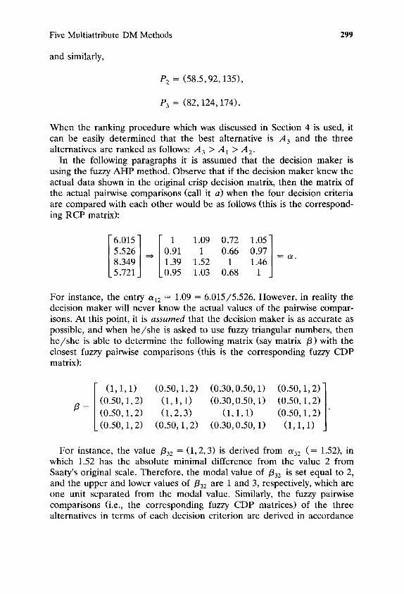
P3 = (82,124,174).

When the ranking procedure which was discussed in Section 4 is used, it can be easily determined that the best alternative is A 3 and the three alternatives are ranked as follows: A 3 > A 1 > A 2.

In the following paragraphs it is assumed that the decision maker is using the fuzzy AHP method. Observe that if the decision maker knew the actual data shown in the original crisp decision matrix, then the matrix of the actual pairwise comparisons (call it a) when the four decision criteria are compared with each other would be as follows (this is the corresponding RCP matrix):

6.0151 [ 1 1.09 0.72 1.05] 5 .526 | ~ |0 .91 1 0.66 0 .97 | = 8.349 | | 1.39 1.52 1 1 .46 | 5.721] L0.95 1.03 0.68 1 ]

OZ.

For instance, the entry o~12 = 1.09 = 6.015/5.526. However, in reality the decision maker will never know the actual values of the pairwise comparisons. At this point, it is assumed that the decision maker is as accurate as possible, and when he / she is asked to use fuzzy triangular numbers, then he / she is able to determine the following matrix (say matrix /3) with the closest fuzzy pairwise comparisons (this is the corresponding fuzzy CDP matrix):

/ 3 =

(1,1, 1) (0.50, 1,2) (0.30, 0.50, 1) (0.50, 1,2) ] (0.50, 1, 2) (1, 1, 1) (0.30, 0.50, 1) (0.50, 1, 2) | (0.50, 1, 2) (1, 2, 3) (1, 1, 1) (0.50, 1,2) 1" (0.50, 1,2) (0.50, 1,2) (0.30,0.50, 1) (1, 1, 1) J

For instance, the value /332 = (1, 2, 3) is derived from oL32 ( = 1.52), in which 1.52 has the absolute minimal difference from the value 2 from Saaty's original scale. Therefore, the modal value of /332 is set equal to 2, and the upper and lower values of /332 a r e 1 and 3, respectively, which are one unit separated from the modal value. Similarly, the fuzzy pairwise comparisons (i.e., the corresponding fuzzy CDP matrices) of the three alternatives in terms of each decision criterion are derived in accordance


with the Saaty scale and are as follows:

4.454 ] 3.647 | 6.232_1

3.253 ] 8.450 | 7.273 J

3.987 ] 1.447 ] 2.496.]

5.816] 2.189 =~ 4.736

1 1.22 0.71] 0.82 1 0.59 1.41 1.69 1

(1, 1, 1) (0.50, 1, 2) (0.50, 1,2) (1, 1, 1)

(1,2, 3) (2, 3, 4)

1 0.38 0.45] 1 ,16j

2.22 0.86

(1, 1, 1) (0.25,0.30,0.50) (2, 3, 4) (1, 1, 1) (1, 2, 3) (0.50, 1,2)

1 2.76 1.60] 0.36 1 0.58 l 0.63 1.72 1

(1, 1, 1) (2, 3, 4) (0.25, 0.30, 0.50) (1, 1, 1)

(0.30,0.50,1) (1,2,3)

1 2.66 1.23] 0.38 1 0.46] 0.81 2.17

(0.30, 0.50, 1) ] (0.30, 0.50, 1) 1'

(1, 1,1)

(0.30, 0.50, 1) ] (0.50, 1,2) 1'

(1, 1,1)

(1,2,3) ] (0.30,0.50, 1) ,

(1,1,1)

(1,1,1) (2,3,4) (0.50,1,2) ] = (0.25, 0.30, 0.50) (1, 1, 1) (0.30, 0.50, 1) ].

(0.50, 1, 2) (1, 2, 3) (1, 1, 1)

Next, the eigenvector approach and normalization procedure are applied to the above fuzzy reciprocal matrices in order to derive the relative preference values of the alternatives in terms of the criteria, along with the weights of importance of the four decision criteria. Therefore, the derived fuzzy decision matrix (which we assume the decision maker has estimated) is as follows:

C1 C 2 (0.09, 0.22, 0.69) (0.08, 0.23, 0.61)

(0.13, 0.29, 0.67) (0.10, 0.17, 0.35) (0.10, 0.22, 0.52) (0.24, 0.47, 0.90) (0.24, 0.49, 0.84) (0.16, 0.36, 0.66)

C3 C 4 (0.11, 0.32, 0.73) (0.08, 0.23, 0.61)

A 1 A2 A3

(0.29, 0.55, 0.98) (0.23, 0.46, 0.91) (0.09,0.16,0.34) (0.09,0.16,0.36) (0.14, 0.29, 0.60) (0.16, 0.38, 0.81)


The final priority scores P1, P2, and P3 of the three alternatives are derived as before and are as follows:

P1 = (0.09, 0.26, 0.72) × (0.12, 0.28, 0.66) + (0.08, 0.22, 0.60)

× (0.09, 0.16, 0.34)

+ (0.11,0.30, 0.72) x (0.28, 0.54, 0.97) + (0.08, 0.22, 0.60)

× (0.22, 0.45, 0.90)

= (0.070, 0.384, 1.946),

and similarly,

P2 = (0.045, 0.245, 1.376),

P3 = (0.063, 0.371, 1.914).

When these priority values are ranked as before, then the three alternatives are ranked as follows: A~ > A 3 > A 2. That is, alternative A 1 turns out now to be the best one. Obviously, this is in contradiction with the results derived when the fuzzy WSM was applied at the beginning of this illustrative example.

At the same time, it can also be observed that the entire ranking order of the alternatives as derived by the fuzzy WSM and the fuzzy AHP has also changed (that is, from A 3 > A 1 > A 2 to A 1 > A 3 > A2). Therefore, a contradiction occurs between fuzzy WSM and fuzzy AHP when one compares the entire ranking orders of the three alternatives for this illustrative example.

It is possible that the best alternative derived from the fuzzy WSM and other fuzzy methods is identical but the remaining alternatives change their orders. The revised (i.e., ideal-mode) AHP, WPM, and TOPSIS methods can be examined as above, and it can be similarly demonstrated that they also yield contradictions when a single-dimensional environment is assumed and the fuzzy WSM is used as the norm.

6.2. Using the Second Evaluative Criterion

Similarly to Section 6.2, the use of the second evaluative criterion is best illustrated by an example.

EXAMPLE 6-2 As with the previous example, suppose that a decision problem with four criteria and three alternatives has the following decision


matrix (again, i t is assumed that these values are unknown to the decision maker):

A 1

A2 A3

C 1 C 2 C 3 C 4 2.885 3.987 2.434 4.894

8.283 7.851 1.064 4.554 5.284 8.626 4.161 3.750 1.358 2.905 8.501 4.888

When one generates the fuzzy triangular numbers as before and pro- ceeds as in the previous example, it can be easily shown that the corresponding fuzzy decision matrix (which we assume the decision maker can derive for this problem) is as follows:

A 1

A2 A3

C1 C2 C3 C4 (0.08,0.18,0.47) (0.11,0.30,0.74) (0.08,0.18,0.47) (0.13,0.35,0.82)

(0.35, 0.59, 0.91) (0.21, 0.32, 0.57) (0.06, 0.09, 0.13)

(0.22, 0.43, 0.83) (0.06, 0.08, 0.11) (0.22, 0.43, 0.83) (0.20, 0.31, 0.54) (0.09, 0.14, 0.26) (0.38, 0.62, 0.94)

(0.13,0.33,0.84) (0.13,0.33,0.84) (0.13,0.33,0.84)

Also, the final priority scores P1, P2, and P3 of the three alternatives can be shown to be as follows:

P1 = (0.073,0.361,1.889),

P2 = (0.073,0.355,1.824),

P3 = (0.061,0.284,1.388).

Evidently, alternative A 1 is the best one. Next, alternative A 3 (which is not the best one) in the original matrix is

replaced by A' 3, which is worse than the original A 3. The performance values of A' 3 are the same as in the original alternative A 3 except that the third value in terms of criterion C3, 8.501, is replaced by the least one, 1.064. Thus, the original matrix of crisp numbers is modified as follows:

..41

A2 A;

C 1 C 2 C 3 C 4 2.885 3.987 2.434 4.894

8.283 7.851 1.064 4.554 5.284 8.626 4.161 3.750 1.358 2.905 1.064 4.888


In order to test the stability of the fuzzy AHP method, the same procedure as above is repeated in order to determine the best alternative. The new fuzzy decision matrix can be shown to be as follows:

A 1

A2 M' 3

C 1 C 2 C 3 C 4 (0.08, 0.18, 0.47) (0.11, 0.30, 0.74) (0.08, 0.18, 0.47) (0.13, 0.35, 0.82)

(0.35, 0.59, 0.91) (0.21, 0.32, 0.57) (0.06, 0.09, 0.13)

(0.22, 0.43, 0.83) (0.10, 0.17, 0.29) (0.13,0.33, 0.84) (0.22, 0.43, 0.83) (0.45, 0.67, 0.97) (0.13, 0.33, 0.84) (0.09, 0.14, 0.26) (0.10, 0.17, 0.29) (0.13, 0.33,0.84)

The final priority scores now become

P1 = (0.077, 0.377, 1.872),

P2 = (0.092, 0.418, 2.030),

P~ = (0.040, 0.205, 1.082).

From the above scores it is obvious that now the best alternative is A 2. This result is in contradiction with the earlier result, namely that the best alternative is A 1. This analysis indicates that a contradiction may occur when the fuzzy AHP (original version) is used and a nonoptimal alternative is replaced by a worse one. In a similar manner it can be shown that the ideal AHP, WPM, and TOPSIS methods may also fail when they are tested in a similar manner.

7. COMPUTATIONAL EXPERIMENTS

The previous fuzzy decision-making methods were evaluated by generat- ing test problems which were treated like Examples 6-1 and 6-2 and then recording the contradiction rates. These experiments were conducted in an attempt to examine the performance of the previously mentioned fuzzy decision-making methods in terms of the two evaluative criteria. There- fore, the three contradiction rates which were considered in these computational experiments are summarized as follows:

R l l is the rate at which the fuzzy WSM and another fuzzy method disagree in the indication of the best alternative.

R12 is the rate at which the fuzzy WSM and another fuzzy method disagree on the entire ranking of the alternatives.

R21 is the rate at which a method changes the indication of the best alternative when a nonoptimal alternative is replaced by a worse alternative.


The c o m p u t e r p r o g r a m was wr i t t en in FORTRAN and run on an I B M 3090 m a i n f r a m e compute r . A to ta l of 400 (i.e., 10 a l te rna t ives × 10 cr i ter ia × 4 me thods ) cases were examined with 3, 5, 7, . . . , 19, 21 a l te rna- tives and 3 ,5 ,7 , . . . , 19,21 cr i ter ia . T h r e e kinds of con t rad ic t ion ra tes were r e c o r d e d for each case by runn ing each case with 500 r a n d o m repl ica t ions .

As s ta ted in the prev ious sect ions, it was a s sumed that the dec is ion m a k e r d id not know the ac tual values o f the a l te rna t ives in t e rms of the decis ion cr i ter ia o r the weights of i m p o r t a n c e of the dec is ion cr i ter ia . F o r the pu rposes o f these s imula t ions , the or iginal i m p o r t a n c e measu re s of the a l te rna t ives in t e rms of the decis ion cr i ter ia were g e n e r a t e d r andomly within the interval [1, 9] (which is the interval o f the values accord ing to the or iginal Saa ty scale). The fuzzy A H P (or iginal and revised), W P M , and TOPSlS m e t h o d s were then examined in t e rms o f the two evaluat ive cr i te r ia in a m a n n e r s imi lar to the p r o c e d u r e s desc r ibed in E x a m p l e s 6-1 and 6-2. The compu ta t i on a l resul ts a re dep ic t ed in F igures 4 to 8 and are also discussed in the fol lowing two subsect ions.

7.1. Description of the Computational Results

In F igures 4 to 8 the fuzzy A H P , fuzzy revised A H P , fuzzy W P M , and fUZzy TOPSIS are d e n o t e d as F - A H P , F - R A H P , F - W P M , and F - T O P S I S ,

.35

.3

.25

e- . 2 o

-o 2 .15 o

O

.1

.05

. . . . . . . . . . . . . . . . . . . . . . . . . . . . . . . . . . . . . . . . . . . . . . . . . . . . . . . . . . . . . . . . . . . . . . . .

.......... ~ ......................... i " 2 ~ ......... i .................................................... ? ......... '~ ........... i ........................ ! ....................... ~ ......................... f ..........

, i 1 1 2 1 ' i i . ............. . i ............. .72 ............ i ; . ............. 2 .... 4 6 8 10 12 14 16 18 20

Number of CriteriG Figure 4. Contradiction rate R l l when the number of alternatives is equal to 3.

Five M u l t i a t t r i b u t e D M M e t h o d s 305

.55 . . . . . . . . . . . . . I . . . . . . ' '

. 5 .................................................................................................................... ~ g c i / ~ N i ~ ............................................... ~ ......................... ~ ...........

. , ~ . . . . . . . ~ ....................... ~ ......................... ~ ......................... , . . . . . . . . . . . . . . . . . + ........................ { . . . . . . . . .~ .~,~ . . . . . . . . . ,~,~,,. . . , ,~.-.: : :~." ~--_......

. ' ~ .......... ! .......................... i ......................... i - - - " : ; ~ , - - " : : : ' - i ......................... i ......................... i ......................... i ......................... i ......................... ~ ..........

*~ i i ,r" i ! i i ! i i "5 .35 a: i !../ i i ~-uPM i i

g . 3 . .-.. . . . .+...-.: . . . . . . . . . . . . . . . . . . . . . . . . . . . . . . . . . . . . . . . . . . . . . . . . . . . . . . . . . . . . . . . . . . . . . . . . . . . . . . . . . . . . . . . . . . . . . . . . . . . . . . . - - ~ " " " ~ - i . . . . . . ~ . . . . . . . . . . . . ~ ..................... ~ ........................ i .......... "~.o

.25

g . 2

.15

F-RRHP :

i

° ~ ........... i ........................................................................................................ i ....................... ~ .................................................... i ......................... i ......... 0 , i . . . . . . . . . . . . i . , . i . . . . . . i . . . . i .

4 6 8 10 12 14 16 18 20

N u m b e r of Criteria

F i g u r e 5. C o n t r a d i c t i o n r a t e R l l w h e n t h e n u m b e r o f a l t e r n a t i v e s is e q u a l to 21.

.1

.08

.06 .£ *a

"& .04- 0

.02

i ! F-WPM :~

i .... ~ " - ' k . ~ - ~ e ! i ....

:i J ! \ / ! i ....

....... i ................ i .2 i ......... - ......... " i i . . . . . . . . . i i i i i :

4- 6 8 10 12 14 16 18 20

N u m b e r of Criterio

F i g u r e 6. C o n t r a d i c t i o n r a t e R21 w h e n t h e n u m b e r o f a l t e r n a t i v e s is e q u a l to 3.


.2 i ¸ i . . . . . i . . . . . . . F-WPM

.~.. 15 . . . . . . . . . . . i . . . . . . . . . . . . . . . . . . . . . . . . . . , ............................................................................................................ ~ - - - - , . . . - ~

c~ c -

O

i !

0 i F -TOPSTS i i F-RHP i ¢,D i - F'-RRHP

. 0 ~ S - ~ .......... ~ .......................................................................... ~ ......................... : ...................... i .......................... ~ .........

4 8 8 10 12 14 16 18 20

Number of Criteria

Figure 7. Contradiction rate R21 when the number of alternatives is equal to 2l.

.55 .~ f . . . . . . i . . . . , -o=~i " T T t

.4s ~ i ..-"""i "i ........ -""i :: i

i . 1 5 .......... i .................................................... i ..................................................................................................... i ............................................................

' ........................................................................................................... i ....................... 7 ......................................................................................... . 0 s ........... i ......................... i ......................... ~ .......................... i ......................... ! ......................... :i ......................... ! ..............................................................

0 , i . , . i , . . i . , , " , , , i . . , i . . . i . . . . . . .

4 6 8 10 12 14 16 18 20

.¢ q J

S .35 n ~

g .3 T o

.___ ~ .25

Number of Criteria Figure 8. Contradiction rate R12 when the number of alternatives is equal to 3.


respectively. The computational results suggest that the contradiction rate RI! increases as the number of alternatives increases. For a more trans- parent illustration, Figures 4 and 5 depict the results only for the cases where the number of alternatives is equal to 3 and 21. These results reveal that the rate of change of the indication of the best alternative increases as the number of alternatives increases, no matter which method is used. However, the number of criteria does not seem to be important.

For the contradiction rate R21, which indicates changes of the best alternative when a nonoptimal alternative is replaced by a worse one, it can be seen from the plots in Figures 6 and 7 that the fuzzy revised (i.e., ideal-mode) AHP is slightly better than the other methods.

Similarly, the contradiction rate R12, which indicates changes in the entire ranking of alternatives between the fuzzy WSM and other methods, shows similar behavior. In this case only the results for number of alternatives equal to 3 are shown (in Figure 8). This is because the results for rate R12 when the number of alternatives is 21 were equal to 100% (or very near that value).

Despite the increasing inaccuracy of these fuzzy methods when the decision-making problems become more complex, it can be seen from these graphs that the fuzzy revised AHP is better than any other fuzzy decision-making method in most cases. This results turns out to be in agreement with the results originally reported in [23] (which examined the same problems in a crisp setting). However, now the fuzzy WPM becomes the worst method in terms of the contradiction rate R21 (it was the second best method in the crisp setting).

7.2. Findings of the Simulation Experiments

The results derived from the computational experiments lead to some interesting observations. First, none of the fuzzy decision-making methods examined in this study is perfectly effective in terms of both evaluative criteria. The results indicate that each method yields different rates of contradiction.

Secondly, the results reveal that the contradiction rates increase when the number of alternatives increases. That is, the methods are less accurate when the decision-making problems become more complex.

Finally, it appears that the revised fuzzy AHP is the best method in most cases, although the difference in performance may be small in certain cases. From these results, the fuzzy revised AHP has the smallest contradiction rates in terms of both evaluative criteria. As was stated in the previous subsection, this should not come as a surprise to anyone.

At this point it should also be stated that we also experimented with more scales for quantifying the pairwise comparisons. In particular, we


considered two geometric scales introduced by Lootsma [17] in which the parameter y was equal to 0.50 and 1.00. However, the derived contradiction rates were significantly higher than when the Saaty scale was used, and thus these results were not plotted. For a deeper analysis of some families of scales for quantifying pairwise comparisons, the interested reader may want to see [29].

In summary, the findings of this study reveal that some methods are better than others in some cases even though none of the methods is perfectly accurate. This study gives an experimentally proved suggestion that some fuzzy decision-making methods are more effective than others in solving real-life fuzzy multiattribute decision-making problems.

8. CONCLUDING REMARKS

The previous analyses reveal that none of the five fuzzy decision-making methods is completely perfect in terms of both evaluative criteria. Differ- ent contradiction rates are yielded when these methods are tested according to the two evaluative criteria. The fuzzy WSM could be the simplest method to solve single-dimensional decision-making problems. However, the other more systematic approaches- - the fuzzy AHP, the fuzzy RAHP, and the fuzzy TOPS~S--are more capable of capturing a human's appraisal of ambiguity when complex decision-making problems are considered. This is true because pairwise comparisons provide a flexible and realistic way to accommodate real-life data. The experimental results reveal that the fuzzy revised (ideal-mode) AHP is better than the other methods in terms of the previous two evaluative criteria.

It needs to be emphasized here that these fuzzy decision-making pro- cesses are best used as decision tools. Individual decision makers may reach their own solution after applying any one of them. This study provides only a general view of different methods under certain situations. A broader understanding of the characteristics of the methods and evaluative criteria is required for successful solution of real-life fuzzy multicriteria decision-making problems.

References

1. Baas, S. J., and Kwakernaak, H., Rating and ranking of multi-aspect alternatives using fuzzy sets, Automatica 13, 47-58, 1977.

2. Bellman, R. E., and Zadeh, L. A., Decision-making in a fuzzy environment, Management Sci. 17, 212-223, 1970.


3. Belton, V., and Gear, T., On a short-coming of Saaty's method of analytic hierarchies, Omega, 228-230, Dec. 1983.

4. Ben-Arieh, D., and Triantaphyllou, E., Quantifying data for group technology with weighted fuzzy features, Internat. J. Production Res. 30, 1285-1299, 1992.

5. Benayoun, R., Roy, B., and Sussman, N., Manual de reference du programme electre, Note de Synthese et Formation, No. 25, Direction Scientifique SEMA, Paris, 1966.

6. Boender, C. G. E., de Graan, J. G. and Lootsma, F. A., Multi-criteria decision analysis with fuzzy pairwise comparisons, Fuzzy Sets and Systems 29, 133-143, 1989.

7. Bridgman, P. W., DimensionalAnalysis, Yale U.P., New Haven, 1922.

8. Buckley, J. J., Ranking alternatives using fuzzy numbers, Fuzzy Sets and Systems 15, 21-31, 1985.

9. Dubois, D., and Prade, H., Fuzzy Sets and Systems, Academic, New York, 1980.

10. Dubois, D., and Prade, H., Fuzzy real algebra: Some results, Fuzzy Sets and Systems 2, 327-348, 1979.

11. Chen, S. J., and Hwang, C. L., Fuzzy Multiple Decision Making, Lecture Notes in Econom. and Math. Systems 375, Springer-Verlag, New York, 1992.

12. Fishburn, P. C., Additive utilities with incomplete product set: Applications to priorities and assignments, Oper. Res. Soc. of America, 1967.

13. Hwang C. L., and Yoon, K., Multiple Attribute Decision Making: Methods and Applications, Springer-Verlag, New York, 1981.

14. Ichihashi, H., and TiJrksen, I. B., A neuro-fuzzy approach to data analysis of pairwise comparisons, Approx. Reasoning 9, 227-248, 1993.

15. Tseng, T. Y., and Klein, C. M., A new algorithm for fuzzy multicriteria decision making, Approx. Reasoning, 6, 45-66, 1992.

16. Laarhoven, P. J. M., and Pedrycz, W., A fuzzy extension of Saaty's priority theory, Fuzzy Sets and Systems 11, 229-241, 1983.

17. Lootsma, F. A., Numerical scaling of human judgment in pairwise-comparison methods for fuzzy multi-criteria decision analysis, Math. Models Decision Sup- port 48, 57-88, 1988.

18. McCahon, C. S., and Lee, E. S., Comparing fuzzy numbers: The proportion of the optimum method, Approx. Reasoning 4, 159-163, 1990.

19. Miller, D. W., and Starr, M. K., Executive Decisions and Operations Research, Prentice-Hall, Englewood Cliffs, N.J., 1969.

20. Saaty, T. L., The Analytic Hierarchy Process, McGraw-Hill, New York, 1980.

21. Saaty, T. L., Fundamentals of Decision Making and Priority Theory with the AHP, RWS Publications, Pittsburgh, 1994.


22. Tong, R. M., and Bonissone, P."P., A linguistic approach to decision making with fuzzy sets, 1EEE Trans. Systems Man Cybemet. SMC-10(ll), 716-723, 1980.

23. Triantaphyllou, E., and Mann, S. H., An examination of the effectiveness of multi-dimensional decision-making methods: A decision-making paradox, Deci- sion Support Systems 5, 303-312, 1989.

24. Triantaphyllou, E., Pardalos, P. M., and Mann, S. H., A minimization approach to membership evaluation in fuzzy sets and error analysis, J. Optim. Theory Appl. 66, 275-287, 1990.

25. Triantaphyllou, E., and Mann, S. H., An evaluation of the eigenvalue approach for determining the membership values in fuzzy sets, Fuzzy Sets and Systems 35, 295-301, 1990.

26. Triantaphyllou, E., Pardalos, P. M., and Mann, S. H., The problem of determining membership values in fuzzy sets in real world situations, in Operations Research and Artificial Intelligence: The Integration of Problem Solving Strategies (D. E. Brown and C. C. White III, Eds.), Kluwer Academic, 197-214, 1990.

27. Triantaphyllou, E., A quadratic programming approach in estimating similarity relations, IEEE Trans. Fuzzy Systems 1, 138-145, 1993.

28. Triantaphyllou, E., and Mann, S. H., A computational evaluation of the AHP and the revised AHP when the eigenvalue method is used under a continuity assumption, Comput. and Indust. Eng. 26, 609-618, 1994.

29. Triantaphyllou, E., Lootsma, F. A., Pardalos, P. M., and Mann, S. H., On the evaluation and application of different scales for quantifying pairwise comparisons in fuzzy sets, Multi-Criteria Decision Anal. 3, 133-155, 1994.

30. Triantaphyllou, E., A linear programming based decomposition approach in evaluating relative priorities from pairwise comparisons and error analysis, J. Optim. Theory Appl. 84, 207-234, 1995.

31. Triantaphyllou, E., and Mann, S. H., Some critical issues in making decisions with pairwise comparisons, Proceedings of the Third International Symposium on the Analytic Hierarchy Process, George Washington Univ., Washington, 225 -236, 11-13 July 1994.

32. Zadeh, L. A., Fuzzy sets, Inform. and Control 8, 338-353, 1965.

33. Zhu, Q., and Lee, E. S., Comparison and ranking of fuzzy numbers, in Fuzzy Regression Analysis, Omnitech Press, Warsaw, 132-145, 1992.

34. Zimmermann, H. J., Fuzzy Set Theory--and Its Applications, Kluwer Aca- demic, Amsterdam, 1985.

north- development and evaluation of five fuzzy...

Documents