nonperforming loans in asia: determinants and macrofinancial linkages (ewp 574) · 2019-04-03 ·...

ASIAN DEVELOPMENT BANK

NONPERFORMING LOANS IN ASIA: DETERMINANTS AND MACROFINANCIAL LINKAGESJunkyu Lee and Peter Rosenkranz

ADB ECONOMICSWORKING PAPER SERIES

NO. 574

March 2019

ASIAN DEVELOPMENT BANK

ADB Economics Working Paper Series

Nonperforming Loans in Asia: Determinants and Macrofinancial Linkages Junkyu Lee and Peter Rosenkranz

No. 574 | March 2019

Junkyu Lee ([email protected]) is Principal Economist and Peter Rosenkranz ([email protected]) is Economist at the Economic Research and Regional Cooperation Department of the Asian Development Bank (ADB). This paper has been prepared as background material for the Asian Economic Integration Report 2017 theme chapter entitled: The Era of Financial Interconnectedness: How Can Asia Strengthen Financial Resilience?. The authors thank Yasuyuki Sawada, Reiner Martin, and Dominik Peschel, as well as the participants of the International Public AMC Forum (IPAF) Financial Stability Seminar on Managing NPLs in Asia and Europe in Shanghai on 8–10 November 2016 and the IPAF Research Workshop in Manila on 30 May 2017 for helpful comments and suggestions. They also acknowledge Jesson Pagaduan, Ryan Jacildo, Junray Bautista, Alyssa Villanueva, Mara Tayag, and Pilar Dayag for excellent research assistance.

Creative Commons Attribution 3.0 IGO license (CC BY 3.0 IGO)

© 2019 Asian Development Bank6 ADB Avenue, Mandaluyong City, 1550 Metro Manila, PhilippinesTel +63 2 632 4444; Fax +63 2 636 2444www.adb.org

Some rights reserved. Published in 2019.

ISSN 2313-6537 (print), 2313-6545 (electronic)Publication Stock No. WPS190050-2DOI: http://dx.doi.org/10.22617/WPS190050-2

The views expressed in this publication are those of the authors and do not necessarily reflect the views and policies of the Asian Development Bank (ADB) or its Board of Governors or the governments they represent.

ADB does not guarantee the accuracy of the data included in this publication and accepts no responsibility for any consequence of their use. The mention of specific companies or products of manufacturers does not imply that they are endorsed or recommended by ADB in preference to others of a similar nature that are not mentioned.

By making any designation of or reference to a particular territory or geographic area, or by using the term “country” in this document, ADB does not intend to make any judgments as to the legal or other status of any territory or area.

This work is available under the Creative Commons Attribution 3.0 IGO license (CC BY 3.0 IGO) https://creativecommons.org/licenses/by/3.0/igo/. By using the content of this publication, you agree to be bound by the terms of this license. For attribution, translations, adaptations, and permissions, please read the provisions and terms of use at https://www.adb.org/terms-use#openaccess.

This CC license does not apply to non-ADB copyright materials in this publication. If the material is attributed to another source, please contact the copyright owner or publisher of that source for permission to reproduce it. ADB cannot be held liable for any claims that arise as a result of your use of the material.

Please contact [email protected] if you have questions or comments with respect to content, or if you wish to obtain copyright permission for your intended use that does not fall within these terms, or for permission to use the ADB logo.

Corrigenda to ADB publications may be found at http://www.adb.org/publications/corrigenda.

Notes: In this publication, “$” refers to United States dollars. ADB recognizes “Hong Kong” as Hong Kong, China.

The ADB Economics Working Paper Series presents data, information, and/or findings from ongoing research andstudies to encourage exchange of ideas and to elicit comment and feedback about development issues in Asia and thePacific. Since papers in this series are intended for quick and easy dissemination, the content may or may not be fullyedited and may later be modified for final publication.

CONTENTS

TABLES AND FIGURES iv ABSTRACT v I. INTRODUCTION 1 II. LITERATURE REVIEW 7 III. DETERMINANTS OF NONPERFORMING LOANS 9 A. Data 9 B. Model 13 C. Results and Discussion 14 IV. FEEDBACK EFFECTS FROM NONPERFORMING LOANS 19 TO THE REAL ECONOMY AND THE FINANCIAL SECTOR A. Data 19 B. Methodology 21 C. Results and Discussion 22 V. CONCLUDING REMARKS 24 APPENDIX 27 REFERENCES 29

TABLES AND FIGURES

TABLES

1 Bank Nonperforming Loans 2 2 Number of Banks in Sample and Their Share in Commercial Bank Total Assets 10 3 Panel Unit Root Tests 11 4 Summary Statistics, Bank-Level Indicators, 1995–2014 12 5 Summary Statistics, Macroeconomic Indicators, 1995–2014 13 6 Macroeconomic and Bank-Level Determinants of Nonperforming Loans, 1995–2014 16 7 Macroeconomic and Bank-Level Determinants of Nonperforming Loans, 17 Precrisis Period, 1995–2007 8 Macroeconomic and Bank-Level Determinants of Nonperforming Loans, 17 Precrisis Period, 2001–2007 9 Macroeconomic and Bank-Level Determinants of Nonperforming Loans, Postcrisis 18 Period, 2008–2014 10 Panel Unit Root Tests 19 11 Summary Statistics, 1994–2014 20 12 Correlation Matrix, 1994–2014 21 13 Granger Causality Test Results 22 A1 Correlation Matrix, 1995–2014 27 A2.1 Forecast Error Variance Decomposition, Baseline Model 27 A2.2 Forecast Error Variance Decomposition, Specification 2 28 FIGURES

1 Nonperforming Loan Levels and Ratios, Selected Asian Economies 4 2 Sources of Corporate Financing in Emerging Asia 7 3 Logit Transformation of the Nonperforming Loan Ratio 12 4 Distribution of the Level and the Change in Nonperforming Loan Ratio, 1994–2014 20 5 Orthogonalized Impulse Response Functions, Baseline Model 23 6 Orthogonalized Impulse Response Functions, Specification 2 24

ABSTRACT The recent rise of nonperforming loans (NPLs) in some Asian economies calls for close analysis of the determinants, the potential macrofinancial feedback effects, and the implications for financial stability in the region. Using a dynamic panel model, we assess the determinants of the evolution of bank-specific NPLs in Asia and find that macroeconomic conditions and bank-specific factors—such as rapid credit growth and excessive bank lending—contribute to the buildup of NPLs. Further, a panel vector autoregression analysis of macrofinancial implications of NPLs in emerging Asia offers significant evidence for the feedback effects of NPLs on the real economy and financial variables. Impulse response functions demonstrate that a rising NPL ratio decreases gross domestic product growth and credit supply and increases unemployment rate. Our findings underline the importance of considering policy options to swiftly and effectively manage and respond to a buildup of NPLs. The national and regional mechanisms underlying NPL resolution are important for safeguarding financial stability in an increasingly interconnected global financial system. Keywords: dynamic panel model, emerging Asia, financial stability, macrofinancial feedback effects, nonperforming loans, panel vector autoregression model

JEL codes: C32, C33, E44, G21, O16

I. INTRODUCTION

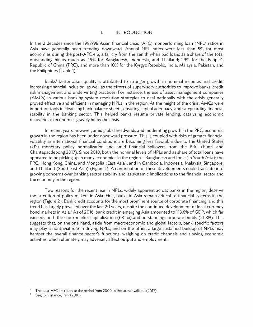
In the 2 decades since the 1997/98 Asian financial crisis (AFC), nonperforming loan (NPL) ratios in Asia have generally been trending downward. Annual NPL ratios were less than 5% for most economies during the post-AFC era, a far cry from the zenith when bad loans as a share of the total outstanding hit as much as 49% for Bangladesh, Indonesia, and Thailand; 29% for the People’s Republic of China (PRC); and more than 10% for the Kyrgyz Republic, India, Malaysia, Pakistan, and the Philippines (Table 1).1

Banks’ better asset quality is attributed to stronger growth in nominal incomes and credit, increasing financial inclusion, as well as the efforts of supervisory authorities to improve banks’ credit risk management and underwriting practices. For instance, the use of asset management companies (AMCs) in various banking system resolution strategies to deal nationally with the crisis generally proved effective and efficient in managing NPLs in the region. At the height of the crisis, AMCs were important tools in cleansing bank balance sheets, ensuring capital adequacy, and safeguarding financial stability in the banking sector. This helped banks resume private lending, catalyzing economic recoveries in economies gravely hit by the crisis.

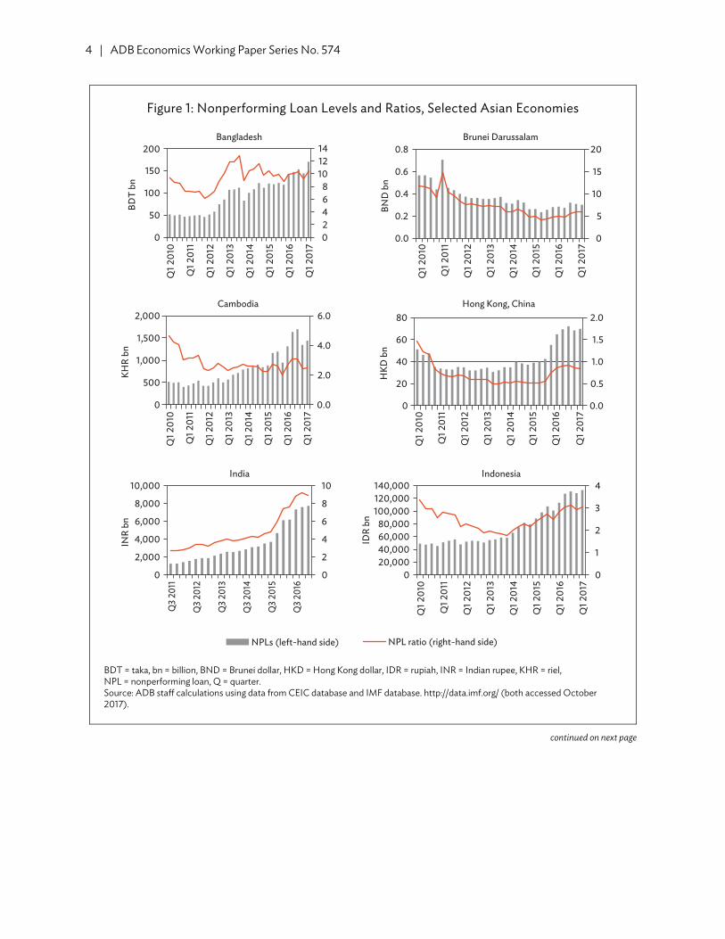
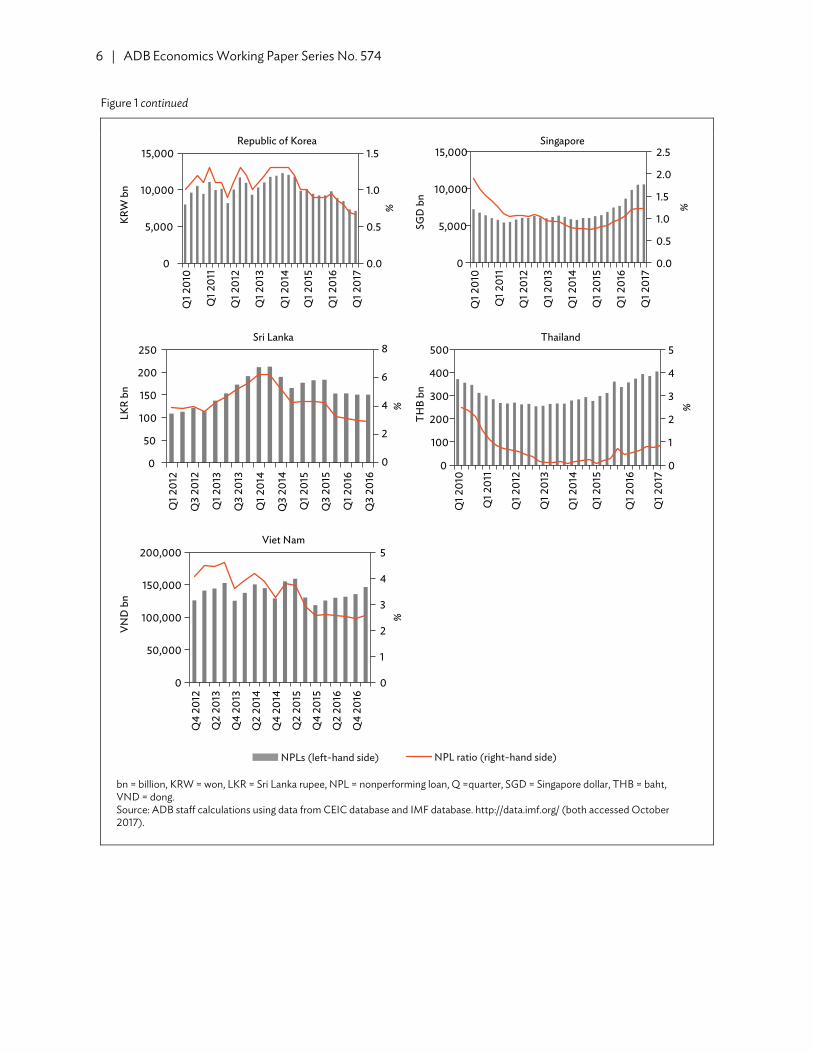
In recent years, however, amid global headwinds and moderating growth in the PRC, economic growth in the region has been under downward pressure. This is coupled with risks of greater financial volatility as international financial conditions are becoming less favorable due to the United States (US) monetary policy normalization and amid financial spillovers from the PRC (Punzi and Chantapacdepong 2017). Since 2010, both the nominal levels of NPLs and as share of total loans have appeared to be picking up in many economies in the region—Bangladesh and India (in South Asia); the PRC; Hong Kong, China; and Mongolia (East Asia); and in Cambodia, Indonesia, Malaysia, Singapore, and Thailand (Southeast Asia) (Figure 1). A continuation of these developments could translate into growing concerns over banking sector stability and its systemic implications to the financial sector and the economy in the region.

Two reasons for the recent rise in NPLs, widely apparent across banks in the region, deserve the attention of policy makers in Asia. First, banks in Asia remain critical to financial systems in the region (Figure 2). Bank credit accounts for the most prominent source of corporate financing, and this trend has largely prevailed over the last 20 years, despite the continued development of local currency bond markets in Asia.2 As of 2016, bank credit in emerging Asia amounted to 113.6% of GDP, which far exceeds both the stock market capitalization (68.1%) and outstanding corporate bonds (21.8%). This suggests that, on the one hand, aside from macroeconomic and global factors, bank-specific factors may play a nontrivial role in driving NPLs, and on the other, a large sustained buildup of NPLs may hamper the overall finance sector’s functions, weighing on credit channels and slowing economic activities, which ultimately may adversely affect output and employment.

1 The post-AFC era refers to the period from 2000 to the latest available (2017). 2 See, for instance, Park (2016).

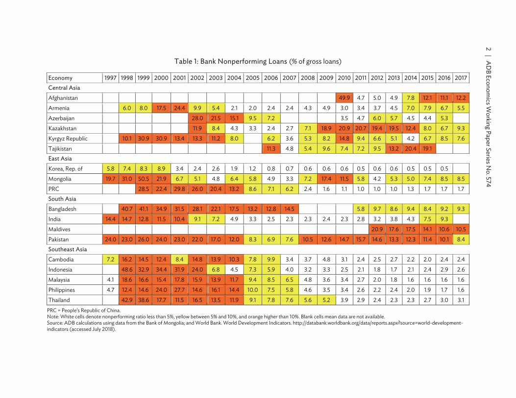
Table 1: Bank Nonperforming Loans (% of gross loans)

Economy 1997 1998 1999 2000 2001 2002 2003 2004 2005 2006 2007 2008 2009 2010 2011 2012 2013 2014 2015 2016 2017Central Asia

Afghanistan 49.9 4.7 5.0 4.9 7.8 12.1 11.1 12.2

Armenia 6.0 8.0 17.5 24.4 9.9 5.4 2.1 2.0 2.4 2.4 4.3 4.9 3.0 3.4 3.7 4.5 7.0 7.9 6.7 5.5

Azerbaijan 28.0 21.5 15.1 9.5 7.2 3.5 4.7 6.0 5.7 4.5 4.4 5.3

Kazakhstan 11.9 8.4 4.3 3.3 2.4 2.7 7.1 18.9 20.9 20.7 19.4 19.5 12.4 8.0 6.7 9.3

Kyrgyz Republic 10.1 30.9 30.9 13.4 13.3 11.2 8.0 6.2 3.6 5.3 8.2 14.8 9.4 6.6 5.1 4.2 6.7 8.5 7.6

Tajikistan 11.3 4.8 5.4 9.6 7.4 7.2 9.5 13.2 20.4 19.1East Asia

Korea, Rep. of 5.8 7.4 8.3 8.9 3.4 2.4 2.6 1.9 1.2 0.8 0.7 0.6 0.6 0.6 0.5 0.6 0.6 0.5 0.5 0.5

Mongolia 19.7 31.0 50.5 21.9 6.7 5.1 4.8 6.4 5.8 4.9 3.3 7.2 17.4 11.5 5.8 4.2 5.3 5.0 7.4 8.5 8.5

PRC 28.5 22.4 29.8 26.0 20.4 13.2 8.6 7.1 6.2 2.4 1.6 1.1 1.0 1.0 1.0 1.3 1.7 1.7 1.7South Asia

Bangladesh 40.7 41.1 34.9 31.5 28.1 22.1 17.5 13.2 12.8 14.5 5.8 9.7 8.6 9.4 8.4 9.2 9.3

India 14.4 14.7 12.8 11.5 10.4 9.1 7.2 4.9 3.3 2.5 2.3 2.3 2.4 2.3 2.8 3.2 3.8 4.3 7.5 9.3

Maldives 20.9 17.6 17.5 14.1 10.6 10.5

Pakistan 24.0 23.0 26.0 24.0 23.0 22.0 17.0 12.0 8.3 6.9 7.6 10.5 12.6 14.7 15.7 14.6 13.3 12.3 11.4 10.1 8.4Southeast Asia

Cambodia 7.2 16.2 14.5 12.4 8.4 14.8 13.9 10.3 7.8 9.9 3.4 3.7 4.8 3.1 2.4 2.5 2.7 2.2 2.0 2.4 2.4

Indonesia 48.6 32.9 34.4 31.9 24.0 6.8 4.5 7.3 5.9 4.0 3.2 3.3 2.5 2.1 1.8 1.7 2.1 2.4 2.9 2.6

Malaysia 4.1 18.6 16.6 15.4 17.8 15.9 13.9 11.7 9.4 8.5 6.5 4.8 3.6 3.4 2.7 2.0 1.8 1.6 1.6 1.6 1.6

Philippines 4.7 12.4 14.6 24.0 27.7 14.6 16.1 14.4 10.0 7.5 5.8 4.6 3.5 3.4 2.6 2.2 2.4 2.0 1.9 1.7 1.6

Thailand 42.9 38.6 17.7 11.5 16.5 13.5 11.9 9.1 7.8 7.6 5.6 5.2 3.9 2.9 2.4 2.3 2.3 2.7 3.0 3.1

PRC = People’s Republic of China. Note: White cells denote nonperforming ratio less than 5%, yellow between 5% and 10%, and orange higher than 10%. Blank cells mean data are not available. Source: ADB calculations using data from the Bank of Mongolia; and World Bank. World Development Indicators. http://databank.worldbank.org/data/reports.aspx?source=world-development-indicators (accessed July 2018).

2 | AD

B Econom

ics Working Paper Series N

o. 574

Nonperforming Loans in Asia: Determinants and Macrofinancial Linkages | 3

Second, given the risks stemming from financial integration in the region, deeper regional and global financial interconnectedness could amplify the propagation of shocks, thereby threatening financial stability. Indeed, the vast literature on contagion and spillovers stresses how financial shocks can be spread through financial linkages via various channels (Forbes 2012). For example, on the back of banking sector interconnectedness through cross-border banking, a shock to one country’s financial sector (such as a sharp increase in nonperforming loans or a deposit run) can cause banks to reduce the supply of credit to other economies as well. Idiosyncratic shocks to the value of investors’ portfolios in one country may also force them to sell assets in other countries to meet margin calls or cash requirements. Kwan, Wong, and Hui (2014) highlight one transmission channel of contagion originating from advanced economies experiencing financial distress (which are lending) to emerging economies (which are borrowing), resulting in pronounced capital outflows from the latter as credit conditions tighten in the former. Park and Shin (2017) illustrate a similar channel, showing that the (borrowing) exposure of emerging market economies to advanced economies that are experiencing a financial crisis significantly explained capital outflows from these emerging market economies during the global financial crisis.

Therefore, the recent rise of NPLs in some Asian economies calls for close analysis of the determinants, its potential macrofinancial feedback effects, and the implications for financial stability in the region. An investigation of the macroeconomic and bank-specific factors that drive NPLs in Asia helps to enhance the understanding of the nature and characteristics of NPLs, thereby facilitating the design of possible policy measures to address a buildup of NPLs. Further, we estimate macrofinancial feedback effects of NPLs to economies’ overall financial systems and real economic sectors to explore the costs associated with NPLs. Our analysis highlights the negative feedback effects both on the financial sector and the real economy, calling for mitigating policy action.

Results reveal that output, unemployment, and inflation influence NPLs considerably, a finding consistent across the alternative model specifications. Although the magnitude is relatively small, intensified global risk aversion and tighter financial conditions, as captured by a rising VIX, are associated with heightened credit risks in the form of higher NPLs.3 Bank-specific factors are found to have a statistically significant, albeit relatively small, effect on credit risk. In particular, low-capitalized, less profitable banks—and those with more risk appetite—tend to have higher NPLs. The findings of the Granger causality tests confirm the substantial feedback effects of NPLs on the economy’s overall financial system and real sector. Impulse response functions show that the impact of a rise in NPLs on economic and financial variables is sizable. It also shows that over 3 years, a 1 percentage point increase in the NPL ratio leads to a cumulative effect of about a 0.1 percentage point contraction of GDP growth, about a 1.5 percentage point decline in loans growth, and a 0.1 percentage point pickup in unemployment. Our findings underline the importance of considering policy options to swiftly and effectively manage and respond to a buildup of NPLs. National and regional mechanisms underlying NPL resolution are important for safeguarding financial stability in an increasingly interconnected regional and global financial system.

In the paper, section II reviews the literature on the determinants of NPLs in Asia. Section III details data and methodology employed to investigate the macroeconomic and bank-specific determinants of NPLs, section IV discusses the empirical model and its results to estimate the feedback effects of NPLs to the real economy and the banking sector, and the last section concludes and discusses policy implications.

3 VIX is the ticker symbol of the Chicago Board Options Exchange Volatility Index.

4 | ADB Economics Working Paper Series No. 574

Figure 1: Nonperforming Loan Levels and Ratios, Selected Asian Economies

BDT = taka, bn = billion, BND = Brunei dollar, HKD = Hong Kong dollar, IDR = rupiah, INR = Indian rupee, KHR = riel, NPL = nonperforming loan, Q = quarter. Source: ADB staff calculations using data from CEIC database and IMF database. http://data.imf.org/ (both accessed October 2017).

NPLs (left-hand side) NPL ratio (right-hand side)

0.0

2.0

4.0

6.0

0

500

1,000

1,500

2,000

Q1 2

010

Q1 2

011

Q1 2

012

Q1 2

013

Q1 2

014

Q1 2

015

Q1 2

016

Q1 2

017

KHR

bn

Cambodia

0.0

0.5

1.0

1.5

2.0

0

20

40

60

80

Q1 2

010

Q1 2

011

Q1 2

012

Q1 2

013

Q1 2

014

Q1 2

015

Q1 2

016

Q1 2

017

HKD

bn

IDR

bn

Hong Kong, China

0

2

4

6

8

10

0

2,000

4,000

6,000

8,000

10,000

Q3 2

011

Q3 2

012

Q3 2

013

Q3 2

014

Q3 2

015

Q3 2

016

INR

bn

India

0

1

2

3

4

020,00040,00060,00080,000

100,000120,000140,000

Q1 2

010

Q1 2

011

Q1 2

012

Q1 2

013

Q1 2

014

Q1 2

015

Q1 2

016

Q1 2

017

Indonesia

02468

101214

0

50

100

150

200

Q1 2

010

Q1 2

011

Q1 2

012

Q1 2

013

Q1 2

014

Q1 2

015

Q1 2

016

Q1 2

017

BDT

bn

Bangladesh

0

5

10

15

20

0.0

0.2

0.4

0.6

0.8

Q1 2

010

Q1 2

011

Q1 2

012

Q1 2

013

Q1 2

014

Q1 2

015

Q1 2

016

Q1 2

017

BND

bn

Brunei Darussalam

continued on next page


Figure 1 continued

bn = billion, CNY = yuan, KZT = tenge, MNT = togrog, MYR = ringgit, NPL = nonperforming loan, PHP = peso, PKR = Pakistan rupee, Q = quarter. Source: ADB staff calculations using data from CEIC database and IMF database. http://data.imf.org/ (both accessed October 2017).

0

10

20

30

40

0

2,000

4,000

6,000

Q1 2

010

Q1 2

011

Q1 2

012

Q1 2

013

Q1 2

014

Q1 2

015

Q1 2

016

Q1 2

017

Q1 2

010

Q1 2

011

Q1 2

012

Q1 2

013

Q1 2

014

Q1 2

015

Q1 2

016

Q1 2

017

Q1 2

010

Q1 2

011

Q1 2

012

Q1 2

013

Q1 2

014

Q1 2

015

Q1 2

016

Q1 2

017

Q1 2

010

Q1 2

011

Q1 2

012

Q1 2

013

Q1 2

014

Q1 2

015

Q1 2

016

Q1 2

017

Q1 2

010

Q1 2

011

Q1 2

012

Q1 2

013

Q1 2

014

Q1 2

015

Q1 2

016

Q1 2

017

%

KZT

bn

Kazakhstan

0

5

10

15

20

0

500

1,000

1,500

Q1 2

010

Q1 2

011

Q1 2

012

Q1 2

013

Q1 2

014

Q1 2

015

Q1 2

016

Q1 2

017

%

MN

T bn

Mongolia

0

1

2

3

4

0

10

20

30

40

%

MYR

bn

Malaysia

0

2

4

6

8

0

50

100

150

200

250

%

PKR

bn

Pakistan

0.0

1.0

2.0

0

1,000

2,000

%

CNY

bn

People's Republic of China

01122334

0

50

100

150

%

PHP

bn

Philippines




Figure 1 continued

bn = billion, KRW = won, LKR = Sri Lanka rupee, NPL = nonperforming loan, Q =quarter, SGD = Singapore dollar, THB = baht, VND = dong. Source: ADB staff calculations using data from CEIC database and IMF database. http://data.imf.org/ (both accessed October 2017).


0.0

0.5

1.0

1.5

2.0

2.5

0

5,000

10,000

15,000

SGD

bn

Singapore

0.0

0.5

1.0

1.5

0

5,000

10,000

15,000

KRW

bn

Republic of Korea

0

1

2

3

4

5

0

50,000

100,000

150,000

200,000

Q4

2012

Q2

2013

Q4

2013

Q2

2014

Q4

2014

Q2

2015

Q4

2015

Q2

2016

Q4

2016

VND

bn

Viet Nam

Q1 2

010

Q1 2

011

Q1 2

012

Q1 2

013

Q1 2

014

Q1 2

015

Q1 2

016

Q1 2

017

Q1 2

010

Q1 2

011

Q1 2

012

Q1 2

013

Q1 2

014

Q1 2

015

Q1 2

016

Q1 2

017

0

1

2

3

4

5

0

100

200

300

400

500

THB

bn

Thailand

0

2

4

6

8

0

50

100

150

200

250

Q1 2

012

Q3

2012

Q1 2

013

Q3

2013

Q1 2

014

Q3

2014

Q1 2

015

Q3

2015

Q1 2

016

Q3

2016

LKR

bn

Sri Lanka

Q1 2

010

Q1 2

011

Q1 2

012

Q1 2

013

Q1 2

014

Q1 2

015

Q1 2

016

Q1 2

017

% %%%

%


Figure 2: Sources of Corporate Financing in Emerging Asia

GDP = gross domestic product. Note: Emerging Asia (excluding Singapore and Hong Kong, China) includes the People’s Republic of China, India, Indonesia, the Republic of Korea, Malaysia, the Philippines, Thailand, and Viet Nam. Sources: ADB, Asian Economic Integration Report 2017, calculations using data from AsianBondsOnline. https://asianbondsonline.adb.org/; International Monetary Fund (IMF). International Financial Statistics. www.imf.org/en/Data; CEIC database; and IMF. World Economic Outlook October 2016 database. https://www.imf.org/external/pubs/ft/weo/2017/01/weodata/index.aspx (all accessed March 2017).

II. LITERATURE REVIEW

The empirical evidence on the determinants of NPLs in Asian economies has been limited and by and large has been relying on country-level analysis. Nevertheless, there is consensus that two groups of factors influence the evolution of NPLs over time. On the one hand, overall macroeconomic conditions, which affect borrowers’ debt servicing capacity, explain credit risk, as confirmed by the literature on major economies. On the other, bank-specific factors, which focus on variables that can possibly signal or influence risk-taking lending practices, also affect each bank’s NPL level.

Much of the empirical evidence on the macroeconomic determinants of credit risk reveals that NPLs exhibit countercyclical behavior (Klein 2013). In particular, income increases when an economy is expanding and real GDP growth is higher, which then improves borrower capacity to repay loans. Hence, default risk is mitigated and NPLs tend to decrease. Conversely, during economic contraction, unemployment tends to rise, leaving borrowers with fewer resources to repay their debts. Default risk tends to pick up and NPLs to increase.4 Other macroeconomic variables found to affect NPLs include exchange rate, interest rate, and inflation.5

4 For example, see Anderson and Sundaresan (2000), Collin-Dufresne and Goldstein (2001), Salas and Saurina (2002),

Rajan and Dhal (2003), Fofack (2005), and Jiménez and Saurina (2005). 5 For example, see Fuentes and Maquieira (2003); IMF (2006); Louzis, Vouldis, and Metaxas (2010); and Nkusu (2011).

0

20

40

60

80

100

120

1996 2006 2016

Corporate bonds Stock market capitalization Bank credit

% o

f GD

P


Roy (2014) investigated the drivers of NPL ratios in India using panel data of five bank groups for the period 1995–2012. The results of the fixed effects model reveal that an increase in the GDP growth rate—both current period and one-period lag—exerts downward pressure on the NPL ratio, while an increase in the real effective exchange rate (currency appreciation) contributes to the buildup of NPLs.

Using panel data from eight commercial banks for the fourth quarter (Q) of 2008 to Q2 2013, Ha, Trien, and Diep (2014) analyzed the macroeconomic determinants of NPL ratios in Viet Nam. Results of the panel regression confirm the countercyclical behavior of Vietnamese NPLs relative to the GDP growth rate. The study also finds that a higher lending rate is likely to increase the level of NPLs. And inflation and exchange rates are found to have statistically insignificant effects on Vietnamese NPLs.

Various studies in the literature have also considered bank-specific factors that affect banks’ asset quality. Klein (2013) summarized the following hypotheses that attempt to explain the relationship between bank-specific factors and NPLs:

(i) bad management hypothesis,6 which argues that banks’ low cost efficiency signals poor management practices, and thus may likely contribute to NPL buildup on the back of poor loan underwriting, monitoring, and control;

(ii) an alternative hypothesis called skimping,7 which contends that high cost efficiency may increase NPLs due to few resources allocated to monitoring lending risks;

(iii) the moral hazard hypothesis,8 which argues that moral hazard incentives exert upward pressure on NPLs by encouraging banks with relatively low capital to increase the riskiness of their loan portfolios; and

(iv) excess lending,9 which explains that higher NPLs can be attributed to banks’ aggressive risk-taking behavior.

Hassan, Ilyas, and Rehman (2015) tested the importance of bank-specific variables along with social factors such as political interference and management competence in driving NPLs in Pakistan’s banking sector. Using survey data from 150 randomly selected bank managers and other credit officers of the top 12 banks of Lahore, Pakistan, the study found that bank-specific factors such as rapid credit growth, poor monitoring, interest, and weak risk assessment played a significant role in the buildup of NPLs.

Karim, Chan, and Hassan (2010) tested the bad management hypothesis proposed by Berger and DeYoung (1997) using Malaysian and Singaporean banks. Employing the stochastic frontier approach to measure bank efficiency and then incorporating it in a Tobit simultaneous equations model, the study found that an increase in bank efficiency decreases NPLs in Malaysia and Singapore’s banking sectors, providing empirical validation of the bad management hypothesis.

6 Williams (2004); Podpiera and Weill (2008); and Louzis, Vouldis, and Metaxas (2010) provide empirical evidence to

support this hypothesis. 7 See, for instance, Rossi, Schwaiger, and Winkler (2005). 8 Berger and DeYoung (1997) and Salas and Saurina (2002) confirm this hypothesis. 9 This is supported by the empirical findings of Salas and Saurina (2002) and Jiménez and Saurina (2005).


Caballero, Hoshi, and Kashyap (2008) explored the engagement of large Japanese banks in misdirected bank lending (“zombie lending”) to financially impaired borrowers (“zombies”). In this scenario, undercapitalized banks roll over loans from existing borrowers that struggle financially in order to avoid these assets being classified as nonperforming. Consequently, unproductive firms receive credit as opposed to more creditworthy and productive firms. While such a behavior keeps the loans artificially performing, it could also contribute to a buildup in NPLs in the long run due to this credit misallocation to unproductive firms.

The above discussed studies focus on either the macroeconomic variables or bank-specific factors driving NPLs, and are performed using a country-level analysis. A number of studies have incorporated both sets of factors and performed the analysis using bank-level data. Most notable among these include Klein (2013), focusing on Central, Eastern, and Southeastern Europe; Nkusu (2011), covering the advanced economies; and Espinoza and Prasad (2010), looking at countries in the Cooperation Council for the Arab States of the Gulf. A major contribution of these studies involves the use of bank-level data and exploiting the unobserved heterogeneity of banks across countries using dynamic panel data methods. All of them provide empirical support for the two sets of factors. In addition, these studies assessed the feedback effects of NPLs to the real side of the economy by employing panel data vector autoregression methods.10

One report that uses a cross-country approach is the panel data analysis of Endut et al. (2013) covering Australia; Bangladesh; the PRC; Hong Kong, China; India; Indonesia; Japan; the Republic of Korea; Malaysia; the Philippines; Singapore, and Thailand. Results of the random effects generalized least squares model reveal that NPL ratios in Asia are influenced by interest rates, inflation rates, and real GDP growth.

The studies reveal several important insights. First, most Asian studies place greater importance on the role of macroeconomic conditions in determining NPLs as opposed to bank-specific factors, and they perform the analysis using aggregate country-level data. Second, there is a limited number of Asian studies that attempt to model the persistence of NPLs as well as their macrofinancial feedback effects. Last, there is no attempt to control for structural changes such as the AFC and global financial crises.

III. DETERMINANTS OF NONPERFORMING LOANS

A. Data

The paper uses panel data of individual banks’ balance sheets from Bankscope and macroeconomic indicators from CEIC. The sample covers annual data for 1995–2014. Bank-level data consists of 165 commercial banks in 17 emerging economies in Asia, and the dataset covers more than 60% of the banking sector’s assets in most of the sample countries (both in Table 2).

10 De Bock and Demyanets (2012) and Messai and Jouini (2013) use a similar approach.


Table 2: Number of Banks in Sample and Their Share in Commercial Bank Total Assets

Country Banks (number) % of Total Assets

Bangladesh 20 78.32

Georgia 8 91.13

Hong Kong, China 3 58.28

India 14 71.96

Indonesia 12 71.10

Japan 13 56.30

Kazakhstan 8 71.39

Korea, Republic of 12 72.43

Kyrgyz Republic 2 43.15

Malaysia 14 89.66

Pakistan 9 79.16

Philippines 5 67.62

PRC 9 52.42

Singapore 2 53.83

Sri Lanka 9 86.97

Thailand 15 85.70

Viet Nam 10 63.73

PRC = People’s Republic of China. Source: Authors’ calculations using data from Bankscope database (accessed February 2016).

The following data are used:

(i) bank-level data, all taken from the Bankscope database, include NPL ratio (ratio of impaired loans to gross loans; 𝑛𝑝𝑙 denotes the logit transformation of the NPL ratio), equity-to-assets ratio (ratio of equity to assets; denoted by 𝑒𝑎𝑟𝑎𝑡𝑖𝑜), return on equity (ratio of net income to average equity; denoted by 𝑟𝑜𝑒), loans-to-deposits ratio (ratio of gross loans to deposits; denoted by 𝑙𝑑𝑟𝑎𝑡𝑖𝑜), loans growth rate (year-on-year growth rate of loans; denoted by Δ𝑙𝑜𝑎𝑛𝑠);

(ii) macroeconomic variables, all taken from CEIC, include the real GDP growth rate (Δ𝑔𝑑𝑝 , unemployment rate (number of unemployed as a percent of the total labor force and Δ𝑢𝑛𝑒𝑚𝑝𝑟𝑎𝑡𝑒, which is the change in unemployment rate), exchange rate (value of local currency per US dollar denoted by 𝑒𝑥𝑟𝑎𝑡𝑒; an increase in the exchange rate means depreciation of the local currency), inflation rate (𝑖𝑛𝑓); and

(iii) a measure of global risk aversion, which is the Standard and Poor’s 500 stock market index (VIX) (denoted by 𝑣𝑖𝑥) taken from the Bloomberg database.


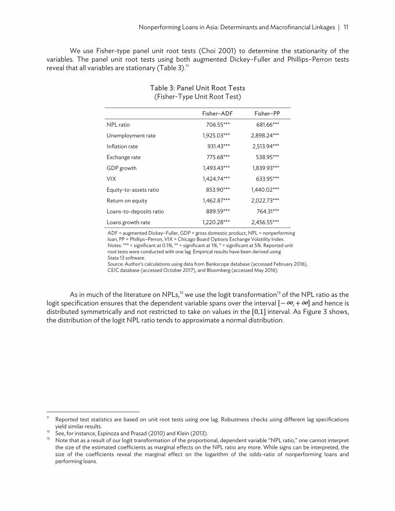
We use Fisher-type panel unit root tests (Choi 2001) to determine the stationarity of the variables. The panel unit root tests using both augmented Dickey–Fuller and Phillips–Perron tests reveal that all variables are stationary (Table 3).11

Table 3: Panel Unit Root Tests (Fisher-Type Unit Root Test)

Fisher–ADF Fisher–PP

NPL ratio 706.55*** 681.66***

Unemployment rate 1,925.03*** 2,898.24***

Inflation rate 931.43*** 2,513.94***

Exchange rate 775.68*** 538.95***

GDP growth 1,493.43*** 1,839.93***

VIX 1,424.74*** 633.95***

Equity-to-assets ratio 853.90*** 1,440.02***

Return on equity 1,462.87*** 2,022.73***

Loans-to-deposits ratio 889.59*** 764.31***

Loans growth rate 1,220.28*** 2,456.55***

ADF = augmented Dickey–Fuller, GDP = gross domestic product, NPL = nonperforming loan, PP = Phillips–Perron, VIX = Chicago Board Options Exchange Volatility Index. Notes: *** = significant at 0.1%, ** = significant at 1%, * = significant at 5%. Reported unit root tests were conducted with one lag. Empirical results have been derived using Stata 13 software. Source: Author’s calculations using data from Bankscope database (accessed February 2016), CEIC database (accessed October 2017), and Bloomberg (accessed May 2016).

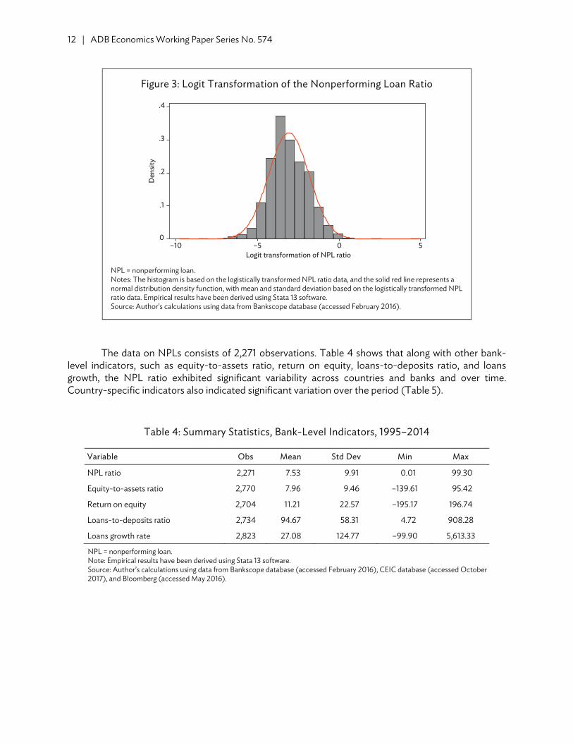
As in much of the literature on NPLs,12 we use the logit transformation13 of the NPL ratio as the logit specification ensures that the dependent variable spans over the interval ∞, ∞ and hence is distributed symmetrically and not restricted to take on values in the 0,1 interval. As Figure 3 shows, the distribution of the logit NPL ratio tends to approximate a normal distribution.

11 Reported test statistics are based on unit root tests using one lag. Robustness checks using different lag specifications

yield similar results. 12 See, for instance, Espinoza and Prasad (2010) and Klein (2013). 13 Note that as a result of our logit transformation of the proportional, dependent variable “NPL ratio,” one cannot interpret

the size of the estimated coefficients as marginal effects on the NPL ratio any more. While signs can be interpreted, the size of the coefficients reveal the marginal effect on the logarithm of the odds-ratio of nonperforming loans and performing loans.


Figure 3: Logit Transformation of the Nonperforming Loan Ratio

NPL = nonperforming loan. Notes: The histogram is based on the logistically transformed NPL ratio data, and the solid red line represents a normal distribution density function, with mean and standard deviation based on the logistically transformed NPL ratio data. Empirical results have been derived using Stata 13 software. Source: Author’s calculations using data from Bankscope database (accessed February 2016).

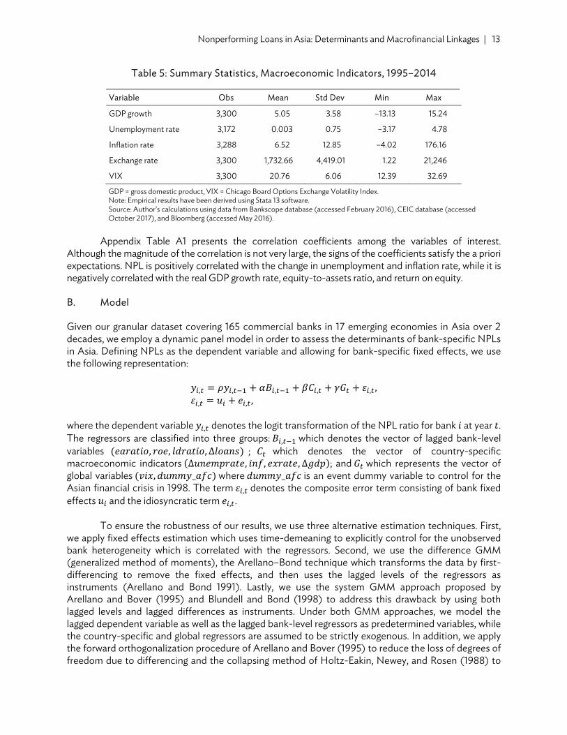
The data on NPLs consists of 2,271 observations. Table 4 shows that along with other bank-level indicators, such as equity-to-assets ratio, return on equity, loans-to-deposits ratio, and loans growth, the NPL ratio exhibited significant variability across countries and banks and over time. Country-specific indicators also indicated significant variation over the period (Table 5).

Table 4: Summary Statistics, Bank-Level Indicators, 1995–2014

Variable Obs Mean Std Dev Min Max

NPL ratio 2,271 7.53 9.91 0.01 99.30

Equity-to-assets ratio 2,770 7.96 9.46 –139.61 95.42

Return on equity 2,704 11.21 22.57 –195.17 196.74

Loans-to-deposits ratio 2,734 94.67 58.31 4.72 908.28

Loans growth rate 2,823 27.08 124.77 –99.90 5,613.33

NPL = nonperforming loan. Note: Empirical results have been derived using Stata 13 software. Source: Author’s calculations using data from Bankscope database (accessed February 2016), CEIC database (accessed October 2017), and Bloomberg (accessed May 2016).

0

.1

.2

.3

.4

Den

sity

–10 –5 0 5Logit transformation of NPL ratio


Table 5: Summary Statistics, Macroeconomic Indicators, 1995–2014


GDP growth 3,300 5.05 3.58 –13.13 15.24

Unemployment rate 3,172 0.003 0.75 –3.17 4.78

Inflation rate 3,288 6.52 12.85 –4.02 176.16

Exchange rate 3,300 1,732.66 4,419.01 1.22 21,246

VIX 3,300 20.76 6.06 12.39 32.69

GDP = gross domestic product, VIX = Chicago Board Options Exchange Volatility Index. Note: Empirical results have been derived using Stata 13 software. Source: Author’s calculations using data from Bankscope database (accessed February 2016), CEIC database (accessed October 2017), and Bloomberg (accessed May 2016).

Appendix Table A1 presents the correlation coefficients among the variables of interest.

Although the magnitude of the correlation is not very large, the signs of the coefficients satisfy the a priori expectations. NPL is positively correlated with the change in unemployment and inflation rate, while it is negatively correlated with the real GDP growth rate, equity-to-assets ratio, and return on equity.

B. Model

Given our granular dataset covering 165 commercial banks in 17 emerging economies in Asia over 2 decades, we employ a dynamic panel model in order to assess the determinants of bank-specific NPLs in Asia. Defining NPLs as the dependent variable and allowing for bank-specific fixed effects, we use the following representation:

𝑦 , 𝜌𝑦 , 𝛼𝐵 , 𝛽𝐶 , 𝛾𝐺 𝜀 , , 𝜀 , 𝑢 𝑒 , ,

where the dependent variable 𝑦 , denotes the logit transformation of the NPL ratio for bank 𝑖 at year 𝑡. The regressors are classified into three groups: 𝐵 , which denotes the vector of lagged bank-level variables 𝑒𝑎𝑟𝑎𝑡𝑖𝑜, 𝑟𝑜𝑒, 𝑙𝑑𝑟𝑎𝑡𝑖𝑜, Δ𝑙𝑜𝑎𝑛𝑠 ; 𝐶 which denotes the vector of country-specific macroeconomic indicators Δ𝑢𝑛𝑒𝑚𝑝𝑟𝑎𝑡𝑒, 𝑖𝑛𝑓, 𝑒𝑥𝑟𝑎𝑡𝑒, Δ𝑔𝑑𝑝 ; and 𝐺 which represents the vector of global variables 𝑣𝑖𝑥, 𝑑𝑢𝑚𝑚𝑦_𝑎𝑓𝑐 where 𝑑𝑢𝑚𝑚𝑦_𝑎𝑓𝑐 is an event dummy variable to control for the Asian financial crisis in 1998. The term 𝜀 , denotes the composite error term consisting of bank fixed effects 𝑢 and the idiosyncratic term 𝑒 , .

To ensure the robustness of our results, we use three alternative estimation techniques. First, we apply fixed effects estimation which uses time-demeaning to explicitly control for the unobserved bank heterogeneity which is correlated with the regressors. Second, we use the difference GMM (generalized method of moments), the Arellano–Bond technique which transforms the data by first-differencing to remove the fixed effects, and then uses the lagged levels of the regressors as instruments (Arellano and Bond 1991). Lastly, we use the system GMM approach proposed by Arellano and Bover (1995) and Blundell and Bond (1998) to address this drawback by using both lagged levels and lagged differences as instruments. Under both GMM approaches, we model the lagged dependent variable as well as the lagged bank-level regressors as predetermined variables, while the country-specific and global regressors are assumed to be strictly exogenous. In addition, we apply the forward orthogonalization procedure of Arellano and Bover (1995) to reduce the loss of degrees of freedom due to differencing and the collapsing method of Holtz-Eakin, Newey, and Rosen (1988) to


control the number of instruments (Roodman 2009). To construct panel-specific serial correlation- and heteroskedasticity-robust standard errors, we also employ the two-step estimation of the covariance matrix in both the difference and system GMM approaches.

C. Results and Discussion

Table 6 presents the results of our estimation. The results reveal that both macroeconomic indicators as well as bank-level variables play a key role in explaining the evolution of banks’ NPL ratios, and this finding appears to be consistent across all model specifications and across the three alternative estimation approaches. The inclusion of bank-level variables increases the explanatory power of the model, both the within- and the between 𝑅-squared (in the fixed effects estimations). The same finding is observed when we control for the Asian financial crisis in 1998—holding bank-level and macroeconomic indicators fixed, banks’ asset quality deteriorated to a large extent during the outbreak of the Asian financial crisis in 1998, and this increase in banks’ NPL ratios is both practically and statistically significant in all the estimation approaches.

In the GMM estimations, we present diagnostic tests and results designed to ensure whether the instruments are valid and whether the estimated dynamic panel data models satisfy the classical assumption of no serial correlation. The Hansen test for overidentifying restrictions reveals that the instruments in both the difference and system GMM satisfy the exogeneity condition—that is, they are uncorrelated with the residuals and hence jointly exogenous instruments. The Arellano–Bond tests for serial correlation reveals that the GMM-estimated models possess serial correlation up to the first lag. This is expected since, by construction, both the difference and system GMM involve differencing which generates serial correlation of order 1 (Wooldridge 2002). The Arellano–Bond test for AR(2) serial correlation finds that there is no serial correlation of order 2, which implies that the assumption of serial independence in the original errors is satisfied.

Across all specifications and estimation methods, the results suggest that banks’ NPL ratios exhibit strong serial correlation. The estimated coefficient of the lagged dependent variable ranges between 0.6 and 0.9. This suggests that a positive shock to NPLs is predicted to have significant lasting effects on the banking system, i.e., NPLs would persistently remain.

The macroeconomic variables contribute to the buildup of NPLs in emerging Asia. The real GDP growth rate, change in the unemployment rate, and inflation rate affect NPLs to a considerable extent, a finding consistent across all alternative estimations. In particular, lower output growth is associated with rising NPLs, confirming the empirical evidence that NPLs tend to behave countercyclically. One of the main transmission channels of this strong link between business cycles and the banking system is unemployment. When the economy slows, unemployment increases and borrowers’ debt servicing capacity suffers, hence the surge in NPLs (Klein 2013; Makri, Tsagkanos, and Bellas 2014). Indeed, our results show that unemployment contributes significantly to higher NPLs. The coefficient of Δ𝑢𝑛𝑒𝑚𝑝𝑟𝑎𝑡𝑒 is both practically and statistically significant across all model specifications and estimation approaches. Inflation, on the other hand, can have an ambiguous effect (Nkusu 2011). Higher inflation can, on the one hand, reduce the real value of outstanding loans thereby making it easier for borrowers to repay debt, or on the other hand, weaken real income when wages are sticky, in which case debt servicing capacity of borrowers deteriorates. The results of our analysis suggest that inflation significantly exhibits the latter behavior.

The VIX and the exchange rate also play a prominent role in explaining the evolution of NPLs among banks in emerging Asia. Although the magnitude is relatively small, intensified global risk


aversion and tighter financing conditions are captured by rising VIX and depreciation of the local currency. They are associated with heightened credit risks in the form of higher NPLs. The VIX and the exchange rate are significantly related to funding conditions and related risks in emerging economies due to the financial channels of the variables. The magnitude of the VIX is much larger than that of the exchange rate.

Moreover, the Asian financial crisis (dummy_afc) is found to have contributed significantly to the buildup of NPLs among emerging Asian banks. For reasons not related to the included macroeconomic indicators and bank-level variables, credit risk in the form of rising NPLs intensified during the outbreak of the Asian financial crisis.

Bank-specific factors are found to have a statistically significant, albeit relatively small, effect on credit risk. In particular, banks with relatively low capital in the form of a smaller equity-to-assets ratio tend to have higher NPLs, holding other factors constant. This supports the moral hazard hypothesis as in Klein (2013) and discussed in Keeton and Morris (1987). According to the hypothesis, low capitalized banks respond to moral hazard incentives by increasing risk appetite in their loan portfolio, thereby increasing NPLs. Risk-taking behavior also explains the positive relationship between the loans-to-deposits ratio and NPLs. The loans-to-deposits ratio measures bank liquidity—it calculates how much funds banks use to create loans from the collected deposits (Makri, Tsagkanos, and Bellas 2014).

Therefore, the more liquid a bank is, the more incentives the bank has to engage in risky behavior and hence to welcome more credit risk. The results suggest strong evidence of a positive relationship between bank liquidity and credit risk, and this finding is robust across the model specifications and alternative estimations. On the other hand, higher bank profitability, as indicated by increasing return on equity, decreases credit risk. This finding supports Makri, Tsagkanos, and Bellas (2014) and Klein (2013) who assert that bank profitability is closely linked with the risk-taking behavior of banks, thus highly profitable banks have fewer incentives to engage in high-risk activities which therefore exerts downward pressure on NPL buildup. Past excessive lending, as measured by the lagged loans growth, is found to contribute to higher NPL buildup among banks in emerging Asia. This finding is statistically significant across all the models.

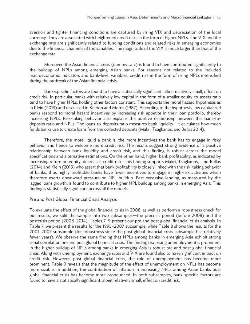
Pre and Post Global Financial Crisis Analysis

To evaluate the effect of the global financial crisis in 2008, as well as perform a robustness check for our results, we split the sample into two subsamples—the precrisis period (before 2008) and the postcrisis period (2008–2014). Tables 7–9 present our pre and post global financial crisis analysis. In Table 7, we present the results for the 1995–2007 subsample, while Table 8 shows the results for the 2001–2007 subsample (for robustness since the post global financial crisis subsample has relatively fewer years). We observe the same finding that NPLs among banks in emerging Asia exhibit strong serial correlation pre and post global financial crisis. The finding that rising unemployment is prominent in the higher buildup of NPLs among banks in emerging Asia is robust pre and post global financial crisis. Along with unemployment, exchange rates and VIX are found also to have significant impact on credit risk. However, post global financial crisis, the role of unemployment has become more prominent. Table 9 reveals that the magnitude of the effect of unemployment on NPLs has become more sizable. In addition, the contribution of inflation in increasing NPLs among Asian banks post global financial crisis has become more pronounced. In both subsamples, bank-specific factors are found to have a statistically significant, albeit relatively small, effect on credit risk.

Table 6: Macroeconomic and Bank-Level Determinants of Nonperforming Loans, 1995–2014

Fixed Effects Difference GMM System GMM

𝑛𝑝𝑙 0.671*** 0.689*** 0.697*** 0.685*** 0.708*** 0.708*** 0.851*** 0.804*** 0.812***

Macroeconomic variables

Δ𝑢𝑛𝑒𝑚𝑝𝑟𝑎𝑡𝑒 0.131*** 0.129*** 0.129*** 0.125*** 0.140*** 0.135*** 0.104*** 0.126*** 0.122***

𝑖𝑛𝑓 0.006 0.010** 0.010** 0.006 0.009*** 0.008*** 0.017*** 0.019*** 0.018***

𝑒𝑥𝑟𝑎𝑡𝑒 0.00005* 0.000 0.000 0.00002 0.00003** 0.00003** 0.000 0.000 0.000

Δ𝑔𝑑𝑝 –0.015** –0.017*** –0.017*** –0.014*** –0.015*** –0.015*** –0.008** –0.011*** –0.011***

𝑣𝑖𝑥 0.008*** 0.007*** 0.006*** 0.006*** 0.005*** 0.004*** 0.006*** 0.005*** 0.005***

𝑑𝑢𝑚𝑚𝑦_𝑎𝑓𝑐 0.383*** 0.266*** 0.306***

Bank-level variables

𝑒𝑎𝑟𝑎𝑡𝑖𝑜 –0.004* –0.005 0.005 0.005 –0.011*** –0.011***

𝑟𝑜𝑒 –0.001* –0.002* 0.002 0.002 –0.001*** –0.0007**

𝑙𝑑𝑟𝑎𝑡𝑖𝑜 0.001*** 0.001*** 0.001* 0.001* 0.001*** 0.001***

Δ𝑙𝑜𝑎𝑛𝑠 0.0005*** 0.0004*** 0.001*** 0.001*** 0.0006*** 0.0006***

No. of observations 1,996 1,770 1,774 1,831 1,686 1,686 1,996 1,764 1,764

𝑅 (within) 0.534 0.540 0.546

𝑅 (between) 0.801 0.967 0.963

No. of banks 165 165 165 165 165 165 165 165 165

No. of instruments 22 81 81 24 96 96

Hansen test 0.136 0.467 0.467 0.899 0.496 0.496

A-B AR(1) test 0.000 0.000 0.000 0.000 0.000 0.000

A-B AR(2) test 0.398 0.278 0.278 0.401 0.306 0.306

GMM = generalized method of moments. Notes: *** = significant at 1%, ** = significant at 5%, * = significant at 10%. Empirical results have been derived using Stata 13 software. Source: Author’s calculations using data from Bankscope database (accessed February 2016), CEIC database (accessed October 2017), and Bloomberg (accessed May 2016).

16 | AD

B Econom

ics Working Paper Series N

o. 574


Table 7: Macroeconomic and Bank-Level Determinants of Nonperforming Loans, Precrisis Period, 1995–2007


𝑛𝑝𝑙 0.531*** 0.531*** 0.868*** 0.726*** 0.896*** 0.717***


Δ𝑢𝑛𝑒𝑚𝑝𝑟𝑎𝑡𝑒 0.103*** 0.114*** 0.112*** 0.157*** 0.112*** 0.114***

𝑖𝑛𝑓 0.009 0.010 0.005 0.005 0.008 0.018***

𝑒𝑥𝑟𝑎𝑡𝑒 0.0001* 0.0001* 0.00008*** 0.00003 –0.000 –0.000

𝑣𝑖𝑥 0.035*** 0.004*** 0.015*** 0.015*** 0.018*** 0.031***


𝑒𝑎𝑟𝑎𝑡𝑖𝑜 –0.002 0.023 –0.006***

𝑟𝑜𝑒 –0.001 -0.0001 –0.002***

𝑙𝑑𝑟𝑎𝑡𝑖𝑜 0.002** 0.002 0.0008

No. of observations 1,135 1,100 1,123 1,087 1,135 1,100

𝑅 (within) 0.479 0.484

𝑅 (between) 0.376 0.423

No. of banks 162 162 162 162 162 162

No. of instruments 15 48 17 53

Hansen test 0.304 0.628 0.406 0.191

A-B AR(1) test 0.000 0.000 0.000 0.000

A-B AR(2) test 0.398 0.687 0.394 0.103


Table 8: Macroeconomic and Bank-Level Determinants of Nonperforming Loans, Precrisis Period, 2001–2007


𝑛𝑝𝑙 0.484*** 0.488*** 0.794*** 0.758*** 0.857*** 0.731***


Δ𝑢𝑛𝑒𝑚𝑝𝑟𝑎𝑡𝑒 0.086** 0.092** 0.081* 0.107*** 0.061* 0.080***

𝑖𝑛𝑓 –0.013 –0.013 –0.0004 –0.004 0.009* 0.013***

𝑒𝑥𝑟𝑎𝑡𝑒 0.00009 0.00007 0.00009*** 0.00006** –0.00002*** –0.00003***

𝑣𝑖𝑥 0.029*** 0.004*** 0.013*** 0.014*** 0.015*** 0.026***


𝑒𝑎𝑟𝑎𝑡𝑖𝑜 –0.023** 0.026 –0.007***

𝑟𝑜𝑒 –0.0005 –0.001 –0.001**




𝑙𝑑𝑟𝑎𝑡𝑖𝑜 0.002*** 0.0005 0.001

No. of observations 899 873 887 860 899 873

𝑅 (within) 0.450 0.461

𝑅 (between) 0.463 0.569

No. of banks 162 162 161 161 162 162


Hansen test 0.324 0.552 0.346 0.199

A-B AR(1) test 0.000 0.000 0.000 0.000

A-B AR(2) test 0.395 0.680 0.396 0.146


Table 9: Macroeconomic and Bank-Level Determinants of Nonperforming Loans, Postcrisis Period, 2008–2014


𝑛𝑝𝑙 0.369*** 0.430*** 0.507*** 0.404*** 0.820*** 0.802***


Δ𝑢𝑛𝑒𝑚𝑝𝑟𝑎𝑡𝑒 0.106** 0.113*** 0.107*** 0.120*** 0.076* 0.109***

𝑖𝑛𝑓 0.014** 0.015** 0.019*** 0.012*** 0.030*** 0.019***

𝑒𝑥𝑟𝑎𝑡𝑒 0.00003 0.000 0.000 0.000 0.000 0.000

𝑣𝑖𝑥 0.0006 –0.002 –0.002 –0.002 –0.004 –0.001


𝑒𝑎𝑟𝑎𝑡𝑖𝑜 –0.0009 0.001 0.0006

𝑟𝑜𝑒 –0.0004 0.0003 0.0002

𝑙𝑑𝑟𝑎𝑡𝑖𝑜 0.00006 0.002*** 0.003***

No. of observations 862 845 708 693 861 845

𝑅 (within) 0.196 0.254

𝑅 (between) 0.814 0.812

No. of banks 153 152 148 148 153 152


Hansen test 0.531 0.463 0.406 0.255

A-B AR(1) test 0.000 0.000 0.000 0.000

A-B AR(2) test 0.410 0.402 0.400 0.299


Table 8 continued


IV. FEEDBACK EFFECTS FROM NONPERFORMING LOANS TO THE REAL ECONOMY AND THE FINANCIAL SECTOR

A. Data

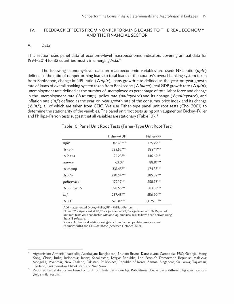
This section uses panel data of economy-level macroeconomic indicators covering annual data for 1994–2014 for 32 countries mostly in emerging Asia.14

The following economy-level data on macroeconomic variables are used: NPL ratio (𝑛𝑝𝑙𝑟) defined as the ratio of nonperforming loans to total loans of the country’s overall banking system taken from Bankscope, change in NPL ratio (Δ𝑛𝑝𝑙𝑟), loans growth rate defined as the year-on-year growth rate of loans of overall banking system taken from Bankscope (Δ𝑙𝑜𝑎𝑛𝑠 , real GDP growth rate (Δ𝑔𝑑𝑝 , unemployment rate defined as the number of unemployed as percentage of total labor force and change in the unemployment rate (Δ𝑢𝑛𝑒𝑚𝑝), policy rate (𝑝𝑜𝑙𝑖𝑐𝑦𝑟𝑎𝑡𝑒 and its change (Δ𝑝𝑜𝑙𝑖𝑐𝑦𝑟𝑎𝑡𝑒), and inflation rate (𝑖𝑛𝑓) defined as the year-on-year growth rate of the consumer price index and its change (Δ𝑖𝑛𝑓), all of which are taken from CEIC. We use Fisher-type panel unit root tests (Choi 2001) to determine the stationarity of the variables. The panel unit root tests using both augmented Dickey–Fuller and Phillips–Perron tests suggest that all variables are stationary (Table 10).15

Table 10: Panel Unit Root Tests (Fisher-Type Unit Root Test)

Fisher–ADF Fisher–PP

𝑛𝑝𝑙𝑟 87.28 *** 125.79***

Δ𝑛𝑝𝑙𝑟 255.52*** 338.11***

Δ𝑙𝑜𝑎𝑛𝑠 95.23*** 146.62***

𝑢𝑛𝑒𝑚𝑝 63.07 88.10***

Δ𝑢𝑛𝑒𝑚𝑝 331.45*** 474.33***

Δ𝑔𝑑𝑝 230.54*** 285.82***

𝑝𝑜𝑙𝑖𝑐𝑦𝑟𝑎𝑡𝑒 172.19*** 258.76***

Δ𝑝𝑜𝑙𝑖𝑐𝑦𝑟𝑎𝑡𝑒 398.55*** 383.53***

𝑖𝑛𝑓 257.45*** 556.20***

Δ𝑖𝑛𝑓 575.81*** 1,075.31***

ADF = augmented Dickey–Fuller, PP = Phillips–Perron. Notes: *** = significant at 1%, ** = significant at 5%, * = significant at 10%. Reported unit root tests were conducted with one lag. Empirical results have been derived using Stata 13 software. Source: Author’s calculations using data from Bankscope database (accessed February 2016) and CEIC database (accessed October 2017).

14 Afghanistan; Armenia; Australia; Azerbaijan; Bangladesh; Bhutan; Brunei Darussalam; Cambodia; PRC; Georgia; Hong

Kong, China; India; Indonesia; Japan; Kazakhstan; Kyrgyz Republic; Lao People’s Democratic Republic; Malaysia; Mongolia; Myanmar; New Zealand; Pakistan; Philippines; Republic of Korea; Samoa; Singapore; Sri Lanka; Tajikistan; Thailand; Turkmenistan; Uzbekistan; and Viet Nam.

15 Reported test statistics are based on unit root tests using one lag. Robustness checks using different lag specifications yield similar results.


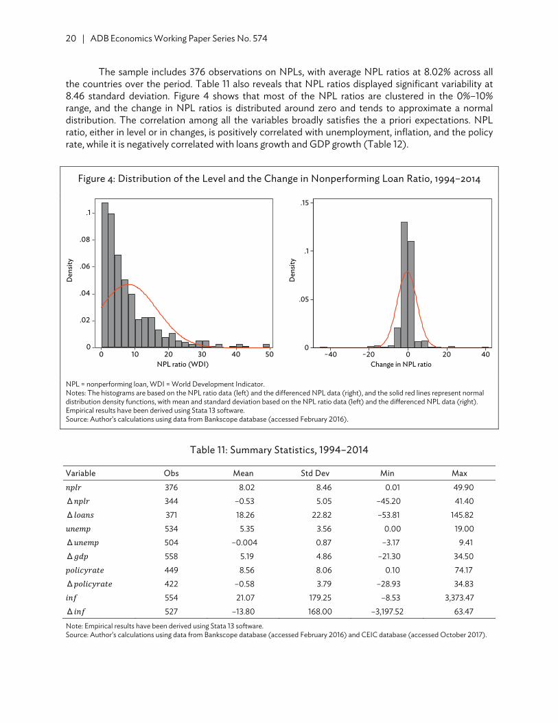
The sample includes 376 observations on NPLs, with average NPL ratios at 8.02% across all the countries over the period. Table 11 also reveals that NPL ratios displayed significant variability at 8.46 standard deviation. Figure 4 shows that most of the NPL ratios are clustered in the 0%–10% range, and the change in NPL ratios is distributed around zero and tends to approximate a normal distribution. The correlation among all the variables broadly satisfies the a priori expectations. NPL ratio, either in level or in changes, is positively correlated with unemployment, inflation, and the policy rate, while it is negatively correlated with loans growth and GDP growth (Table 12).

Figure 4: Distribution of the Level and the Change in Nonperforming Loan Ratio, 1994–2014

NPL = nonperforming loan, WDI = World Development Indicator.Notes: The histograms are based on the NPL ratio data (left) and the differenced NPL data (right), and the solid red lines represent normal distribution density functions, with mean and standard deviation based on the NPL ratio data (left) and the differenced NPL data (right). Empirical results have been derived using Stata 13 software. Source: Author’s calculations using data from Bankscope database (accessed February 2016).

Table 11: Summary Statistics, 1994–2014


𝑛𝑝𝑙𝑟 376 8.02 8.46 0.01 49.90Δ𝑛𝑝𝑙𝑟 344 –0.53 5.05 –45.20 41.40Δ𝑙𝑜𝑎𝑛𝑠 371 18.26 22.82 –53.81 145.82𝑢𝑛𝑒𝑚𝑝 534 5.35 3.56 0.00 19.00Δ𝑢𝑛𝑒𝑚𝑝 504 –0.004 0.87 –3.17 9.41Δ𝑔𝑑𝑝 558 5.19 4.86 –21.30 34.50𝑝𝑜𝑙𝑖𝑐𝑦𝑟𝑎𝑡𝑒 449 8.56 8.06 0.10 74.17Δ𝑝𝑜𝑙𝑖𝑐𝑦𝑟𝑎𝑡𝑒 422 –0.58 3.79 –28.93 34.83𝑖𝑛𝑓 554 21.07 179.25 –8.53 3,373.47Δ𝑖𝑛𝑓 527 –13.80 168.00 –3,197.52 63.47

Note: Empirical results have been derived using Stata 13 software. Source: Author’s calculations using data from Bankscope database (accessed February 2016) and CEIC database (accessed October 2017).

0

.02

.04

.06

.08

.1

Den

sity

0 10 20 30 40 50NPL ratio (WDI)

0

.05

.1

.15

Den

sity

−40 −20 0 20 40Change in NPL ratio


Table 12: Correlation Matrix, 1994–2014

𝒏𝒑𝒍𝒓 𝚫𝒏𝒑𝒍𝒓 𝚫𝒍𝒐𝒂𝒏𝒔 𝒖𝒏𝒆𝒎𝒑 𝚫𝒖𝒏𝒆𝒎𝒑 𝚫𝒈𝒅𝒑 𝒑𝒐𝒍𝒊𝒄𝒚𝒓𝒂𝒕𝒆 𝚫𝒑𝒐𝒍𝒊𝒄𝒚𝒓𝒂𝒕𝒆 𝒊𝒏𝒇 𝚫𝒊𝒏𝒇

𝑛𝑝𝑙𝑟 1.00

Δ𝑛𝑝𝑙𝑟 0.19*** 1.00

Δ𝑙𝑜𝑎𝑛𝑠 –0.22*** –0.04 1.00

𝑢𝑛𝑒𝑚𝑝 –0.03 0.03 0.18*** 1.00

Δ𝑢𝑛𝑒𝑚𝑝 0.12** 0.13** –0.09* 0.14*** 1.00

Δ𝑔𝑑𝑝 –0.11** –0.38*** 0.44*** –0.09** –0.33*** 1.00

𝑝𝑜𝑙𝑖𝑐𝑦𝑟𝑎𝑡𝑒 0.62*** 0.37*** 0.13** 0.15*** 0.11** 0.005 1.00

Δ𝑝𝑜𝑙𝑖𝑐𝑦𝑟𝑎𝑡𝑒 –0.03 0.57*** 0.12** –0.14*** –0.04 –0.03 –0.10* 1.00

𝑖𝑛𝑓 0.30*** 0.38*** 0.23*** 0.02 0.04 –0.19*** 0.63*** 0.12** 1.00

Δ𝑖𝑛𝑓 0.04 0.41*** 0.05 –0.03 –0.02 0.11** –0.30*** 0.43*** –0.66*** 1.00


B. Methodology

To investigate the feedback effects of NPLs on the real economy, we choose to estimate a panel vector autoregression (VAR) model. All variables in the system are endogenous and have potential influence on each other. A VAR framework allows for a structural analysis by estimating impulse response functions for each exogenous shock in the system. For instance, one can estimate dynamic responses of all variables to a shock to the NPL ratio, thereby investigating macrofinancial feedback effects of NPLs and their dynamics. The panel VAR allows for combining the traditional VAR approach with the panel dimension, thereby not only estimating the parameters for an individual economy, but instead for a wider set of economies. It has the following representation:

𝑌 , Π Π 𝑌 , 𝜀 , ,

𝜀 , 𝑢 𝑒 ,

where 𝑌 , is the vector of endogenous variables, 𝜀 , is the composite error term consisting of the country fixed effects 𝑢 and idiosyncratic errors 𝑒 , . In our baseline specification, 𝑌 , consists of four endogenous variables, namely Δ𝑛𝑝𝑙𝑟 , , Δ𝑙𝑜𝑎𝑛𝑠 , , Δ𝑢𝑛𝑒𝑚𝑝 , ( Δ𝑔𝑑𝑝 for specification 2), and Δ𝑝𝑜𝑙𝑖𝑐𝑦𝑟𝑎𝑡𝑒 , , where subscript 𝑖 and 𝑡 denote country 𝑖 and year 𝑡 , respectively. For robustness checks, we estimate the panel VAR both in level and first-difference forms and get qualitatively similar findings. Results of model selection tests developed by Andrews and Lu (2001) reveal that the optimal lag order is 1, hence we include the first lag of each of the four endogenous variables in the estimation. Using the Stata program developed by Abrigo and Love (2015), the panel VAR is estimated using GMM techniques to derive consistent estimates of the parameters. The said program uses the forward orthogonal deviation (Helmert procedure) proposed by Arellano and Bover (1995) to purge the country fixed effects, which are correlated with the regressors due to the lags of the dependent variable. The Helmert procedure transforms the data by subtracting the average of all available future observations. Finally, the program uses GMM-style instruments as proposed by Holtz-Eakin, Newey,


and Rosen (1988). This procedure improves the efficiency of estimates by creating instruments based on observed realizations, with missing observations substituted with zero.

Following Espinoza and Prasad (2010), the identification strategy is based on a Cholesky decomposition with Δ𝑝𝑜𝑙𝑖𝑐𝑦𝑟𝑎𝑡𝑒 appearing first in the ordering, followed by Δ𝑙𝑜𝑎𝑛𝑠, Δ𝑔𝑑𝑝, and finally Δ𝑛𝑝𝑙𝑟. This ordering assumes that the NPL ratio can affect economic growth or credit growth only with a lag and not contemporaneously. This is consistent with the empirical evidence documented in the literature that causality runs initially from economic growth to NPLs. For robustness checks, we also try alternative Cholesky orderings proposed by Klein (2013) and De Bock and Demyanets (2012), which assume that NPLs have a contemporaneous effect on economic activity, while GDP growth, unemployment, and inflation affect NPLs only with a lag. Qualitatively, the results are similar across alternative Cholesky orderings.

C. Results and Discussion

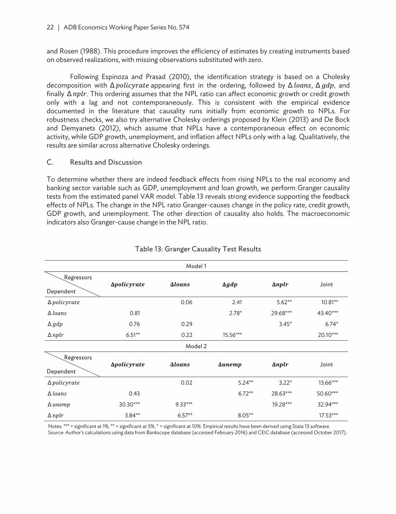
To determine whether there are indeed feedback effects from rising NPLs to the real economy and banking sector variable such as GDP, unemployment and loan growth, we perform Granger causality tests from the estimated panel VAR model. Table 13 reveals strong evidence supporting the feedback effects of NPLs. The change in the NPL ratio Granger-causes change in the policy rate, credit growth, GDP growth, and unemployment. The other direction of causality also holds. The macroeconomic indicators also Granger-cause change in the NPL ratio.

Table 13: Granger Causality Test Results

Model 1

Regressors Dependent

𝚫𝒑𝒐𝒍𝒊𝒄𝒚𝒓𝒂𝒕𝒆 𝚫𝒍𝒐𝒂𝒏𝒔 𝚫𝒈𝒅𝒑 𝚫𝒏𝒑𝒍𝒓 Joint

Δ𝑝𝑜𝑙𝑖𝑐𝑦𝑟𝑎𝑡𝑒 0.06 2.41 5.62** 10.81**

Δ𝑙𝑜𝑎𝑛𝑠 0.81 2.78* 29.68*** 43.40***

Δ𝑔𝑑𝑝 0.76 0.29 3.45* 6.74*

Δ𝑛𝑝𝑙𝑟 6.51** 0.22 15.56*** 20.10***

Model 2

Regressors Dependent

𝚫𝒑𝒐𝒍𝒊𝒄𝒚𝒓𝒂𝒕𝒆 𝚫𝒍𝒐𝒂𝒏𝒔 𝚫𝒖𝒏𝒆𝒎𝒑 𝚫𝒏𝒑𝒍𝒓 Joint

Δ𝑝𝑜𝑙𝑖𝑐𝑦𝑟𝑎𝑡𝑒 0.02 5.24** 3.22* 13.66***

Δ𝑙𝑜𝑎𝑛𝑠 0.43 6.72** 28.63*** 50.60***

Δ𝑢𝑛𝑒𝑚𝑝 30.30*** 9.33*** 19.28*** 32.94***

Δ𝑛𝑝𝑙𝑟 3.84** 6.57** 8.05** 17.53***

Notes: *** = significant at 1%, ** = significant at 5%, * = significant at 10%. Empirical results have been derived using Stata 13 software. Source: Author’s calculations using data from Bankscope database (accessed February 2016) and CEIC database (accessed October 2017).


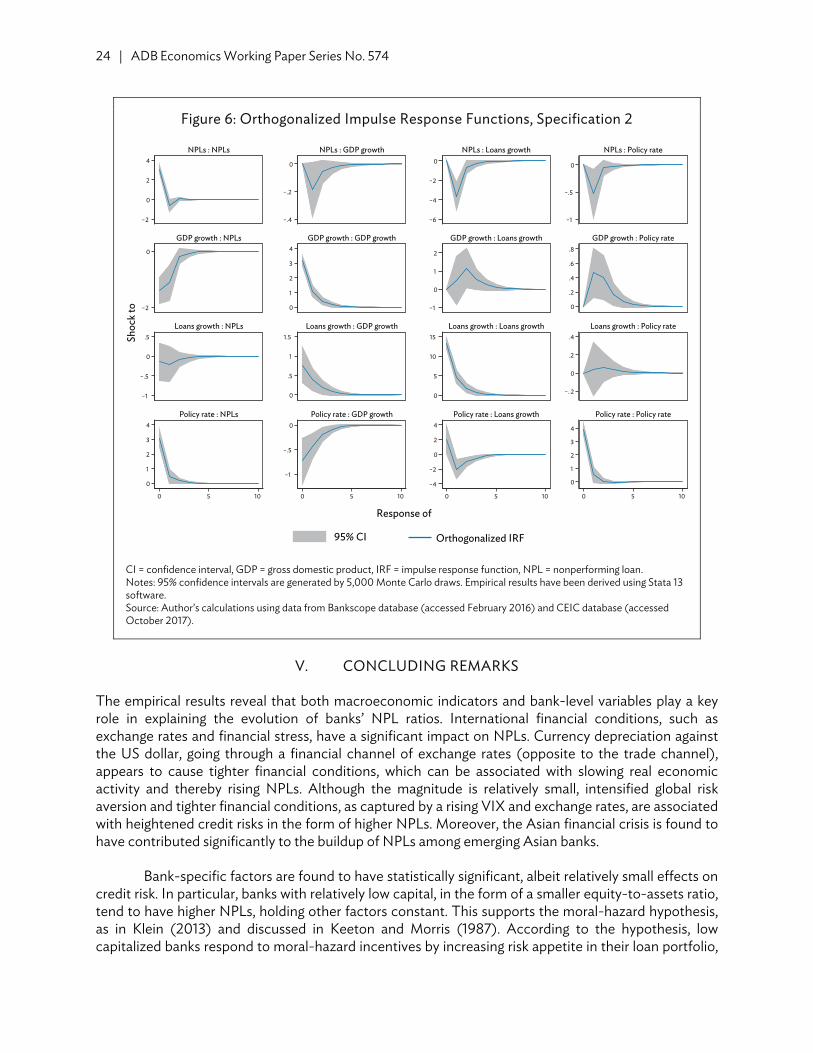
To assess the dynamic behavior of the model, we present the orthogonalized impulse response functions in Figures 5 (baseline model) and 6 (specification 2).

Figure 5: Orthogonalized Impulse Response Functions, Baseline Model

CI = confidence interval, IRF = impulse response function, NPL = nonperforming loan. Notes: 95% confidence intervals are generated by 5,000 Monte Carlo draws. Empirical results have been derived using Stata 13 software. Source: Author’s calculations using data from Bankscope database (accessed February 2016) and CEIC database (accessed October 2017).

The impulse response functions summarize the response of one variable in the system to a shock in another while holding other innovations fixed.16 Our results suggest that a rising NPL ratio decreases GDP growth, credit supply, and the policy rate, and increases unemployment. By magnitude, a one standard deviation shock in the NPL ratio would lead to about 0.18 percentage point contraction in GDP growth rate, about 3.61 percentage point decline in the loan growth rate, and about 0.21 percentage point rise in unemployment after 1 year.17 Over 3 years, a 1 percentage point increase in the NPL ratio leads to a cumulative effect of about a 0.1 percentage point contraction in the GDP growth rate, about a 1.5 percentage point decline in loans growth, and a 0.1 percentage point pickup in unemployment. Higher GDP growth and credit supply both decrease the NPL ratio, while tighter monetary policy and rising unemployment both increase the NPL ratio. 16 See Appendix Tables A2.1 and A2.2 for the underlying forecast error variance decompositions. 17 A one standard deviation shock to the NPL ratio is equal to 3.5 percentage points in the baseline model, and 3.1

percentage points in specification 2.

95% CI Orthogonalized IRF

Shoc

k to

Response of

−2

0

2

4

–.5

0

.5

1

−1

–.5

0

–.5

0

1

2

3

–.1

0

.1

.2

.3

0

.5

1

–.2

0

.2

.4

–.3

–.2

–.1

0

.1

−6

−4

−2

0

−3

−2

−1

0

0

5

10

15

−4

−2

0

2

4

−1

–.5

0

−2

−1.5−1

–.50

–.5

0

.5

0

2

4

0 5 10 0 5 10 0 5 10 0 5 10

NPLs : NPLs

Unemployment rate : NPLs

Loans growth : NPLs

Policy rate : NPLs

NPLs : Unemployment rate

Unemployment rate : Unemployment rate

Loans growth : Unemployment rate

Policy rate : Unemployment rate

NPLs : Loans growth

Unemployment rate : Loans growth

Loans growth : Loans growth

Policy rate : Loans growth

NPLs : Policy rate

Unemployment rate : Policy rate

Loans growth : Policy rate

Policy rate : Policy rate


Figure 6: Orthogonalized Impulse Response Functions, Specification 2

CI = confidence interval, GDP = gross domestic product, IRF = impulse response function, NPL = nonperforming loan. Notes: 95% confidence intervals are generated by 5,000 Monte Carlo draws. Empirical results have been derived using Stata 13 software. Source: Author’s calculations using data from Bankscope database (accessed February 2016) and CEIC database (accessed October 2017).

V. CONCLUDING REMARKS

The empirical results reveal that both macroeconomic indicators and bank-level variables play a key role in explaining the evolution of banks’ NPL ratios. International financial conditions, such as exchange rates and financial stress, have a significant impact on NPLs. Currency depreciation against the US dollar, going through a financial channel of exchange rates (opposite to the trade channel), appears to cause tighter financial conditions, which can be associated with slowing real economic activity and thereby rising NPLs. Although the magnitude is relatively small, intensified global risk aversion and tighter financial conditions, as captured by a rising VIX and exchange rates, are associated with heightened credit risks in the form of higher NPLs. Moreover, the Asian financial crisis is found to have contributed significantly to the buildup of NPLs among emerging Asian banks.

Bank-specific factors are found to have statistically significant, albeit relatively small effects on credit risk. In particular, banks with relatively low capital, in the form of a smaller equity-to-assets ratio, tend to have higher NPLs, holding other factors constant. This supports the moral-hazard hypothesis, as in Klein (2013) and discussed in Keeton and Morris (1987). According to the hypothesis, low capitalized banks respond to moral-hazard incentives by increasing risk appetite in their loan portfolio,

−2

0

2

4

−2

0

−1

−.5

0

.5

0

1

2

3

4

−.4

−.2

0

0

1

2

3

4

0

.5

1

1.5

−1

−.5

0

−6

−4

−2

0

−1

0

1

2

0

5

10

15

−4

−2

0

2

4

−1

−.5

0

0

.2

.4

.6

.8

−. 2

0

.2

.4

0

1

2

3

4

0 5 10 0 5 10 0 5 10 0 5 10

NPLs : NPLs

GDP growth : NPLs

Loans growth : NPLs

Policy rate : NPLs

NPLs : GDP growth

GDP growth : GDP growth

Loans growth : GDP growth

Policy rate : GDP growth

NPLs : Loans growth

GDP growth : Loans growth

Loans growth : Loans growth

Policy rate : Loans growth

NPLs : Policy rate

GDP growth : Policy rate

Loans growth : Policy rate

Policy rate : Policy rate

Shoc

k to

95% CI Orthogonalized IRF

Response of


resulting in increasing NPLs. Risk-taking behavior also explains the positive relationship between loan-to-deposit ratios and NPLs. The loan-to-deposit ratio measures bank liquidity—it calculates how much funds banks use to create loans from the collected deposits (Makri, Tsagkanos, and Bellas 2014).

As such, the more liquid a bank is, the greater its incentive to engage in risky behavior and hence welcome more credit risk. The results suggest strong evidence of a positive relationship between bank liquidity and credit risk, a finding robust across the model specifications and alternative estimations. By contrast, the higher a bank’s profitability, as indicated by increasing return on equity, the lower its credit risk. This finding supports Makri, Tsagkanos, and Bellas (2014) and Klein (2013), who assert that bank profitability is closely linked with risk-taking behavior, thus highly profitable banks have fewer incentives to engage in high-risk activities, exerting downward pressure on NPL buildup. Past excessive lending, as measured by lagged loans growth, is found to contribute to higher NPL buildup among banks in emerging Asia. This finding is statistically significant across all the models. This could relate to the results by Mian, Sufi, and Verner (2017), highlighting the important role of (household) credit supply shocks. They show that a buildup in the household debt-to-GDP ratio is associated with lower GDP growth and higher unemployment.

We also observe the finding that NPLs among banks in emerging Asia exhibit strong serial correlation pre and post global financial crisis. The finding that rising unemployment plays a prominent role in the higher buildup of NPLs among banks in emerging Asia is robust pre and post global financial crisis. Along with unemployment, exchange rates and the VIX are also found to have significant impact on credit risk. However, post global financial crisis, the role of unemployment has become more prominent. Table 9 reveals that the magnitude of the partial effect of unemployment on NPLs has become more sizable. In addition, the contribution of inflation in increasing NPLs among Asian banks post global financial crisis has become more prominent. In both subsamples, banks’ specific factors are found to have a statistically significant, albeit relatively small, effect on credit risk. On the feedback effects from NPLs to economic and financial variables, the results suggest that a rising NPL ratio decreases GDP growth, credit supply, and policy rate, and increases unemployment.

The research results and past episodes of financial crises strongly suggest that rising NPLs must be addressed rapidly and effectively due to an immediate feedback impact on economic and financial variables. NPLs reduce banks’ lending abilities and drag on banks’ profitability (that is, they increase the opportunity cost of capital, since they yield no returns and require capital provisioning, management, and financial resources). Excessive and rapid buildup of NPLs can also cause a credit crunch, leading to a banking crisis, and financing for small and medium-sized enterprises, trade, infrastructure, and households may take a serious hit. Banking instability strongly affects other capital market segments (bonds, equities, and commodities).

Accordingly, the early cleanup of NPLs from bank balance sheets can help restore private sector lending to the real economy and facilitate recovery from a crisis. Effective and preemptive handling of the deterioration of banks’ asset quality can also help inclusive growth, by mitigating the negative impact of NPLs on unemployment and the poor. In addition, the finding that rising unemployment plays a key role in the buildup of NPLs also suggests that, during a crisis, policy measures to mitigate unemployment could be considered part of a comprehensive crisis response package, and decrease the negative impact on financial instability. As such, dealing with a rapid rise of NPLs can be seen as part of either microprudential or macroprudential policies depending on the underlying cause of the vulnerability and country-specific circumstances.


That said, a next step for enhancing financial stability is to determine how policy makers can strengthen Asia’s financial safety nets by effectively and rapidly dealing with asset quality deterioration in bank balance sheets. Measures would include policy options such as recapitalization, corporate debt restructuring, supervisory framework and efforts, as well as employing NPL resolution mechanisms including an AMC option to complement efforts, although not to substitute these. Another policy effort of developing distressed asset markets in Asia, requiring efforts to develop financial markets and their infrastructure, and implement legal and institutional reforms based on country-specific factors, can also be considered.

APPENDIX

Table A1: Correlation Matrix, 1995–2014

𝒏𝒑𝒍 𝚫𝒖𝒏𝒆𝒎𝒑𝒓𝒂𝒕𝒆 𝒊𝒏𝒇 𝒆𝒙𝒓𝒂𝒕𝒆 𝚫𝒈𝒅𝒑 𝒗𝒊𝒙 𝒆𝒂𝒓𝒂𝒕𝒊𝒐 𝒓𝒐𝒆 𝒍𝒅𝒓𝒂𝒕𝒊𝒐 𝚫𝒍𝒐𝒂𝒏𝒔

𝑛𝑝𝑙 1.00 Δ𝑢𝑛𝑒𝑚𝑝𝑟𝑎𝑡𝑒 0.06*** 1.00 𝑖𝑛𝑓 0.05** 0.24*** 1.00 𝑒𝑥𝑟𝑎𝑡𝑒 –0.17*** 0.007 0.05*** 1.00 Δ𝑔𝑑𝑝 –0.06*** –0.43*** –0.17*** 0.06*** 1.00 𝑣𝑖𝑥 0.12*** 0.16*** –0.07*** 0.008 –0.29*** 1.00 𝑒𝑎𝑟𝑎𝑡𝑖𝑜 –0.14*** –0.08*** –0.07*** –0.009 0.05*** –0.02*** 1.00 𝑟𝑜𝑒 –0.22*** –0.12*** 0.14*** 0.06*** 0.17*** –0.08*** –0.006 1.00 𝑙𝑑𝑟𝑎𝑡𝑖𝑜 –0.004 –0.03* –0.03* –0.08*** –0.08*** –0.004 0.06*** –0.13*** 1.00Δ𝑙𝑜𝑎𝑛𝑠 –0.18*** –0.02 0.04** 0.02 0.07** –0.005 0.08*** 0.02 0.005 1.00

Notes: *** = significant at 1%, ** = significant at 5%, * = significant at 10%. Empirical results have been derived using Stata 13 software. Source: Author’s calculations using data from Bankscope database (accessed February 2016), CEIC database (accessed October 2017), and Bloomberg (accessed May 2016).

Table A2.1: Forecast Error Variance Decomposition, Baseline Model

Forecast Horizon Impulse: ∆𝒑𝒐𝒍𝒊𝒄𝒚𝒓𝒂𝒕𝒆 ∆𝒍𝒐𝒂𝒏𝒔 ∆𝒈𝒅𝒑 ∆𝒏𝒑𝒍𝒓

Response: ∆𝒍𝒐𝒂𝒏𝒔 0 0 0 0 01 .0122878 .9877123 0 02 .0295472 .8962381 .0088728 .06534193 .0312659 .8828819 .0151518 .07070054 .0312107 .8806379 .015983 .07216845 .031196 .8802338 .0162574 .07231286 .0311957 .8801723 .0162927 .07233947 .0311961 .8801624 .0163003 .07234118 .0311964 .8801612 .0163012 .07234139 .0311965 .880161 .0163013 .072341210 .0311965 .880161 .0163013 .0723412Response: ∆𝒖𝒏𝒆𝒎𝒑 0 0 0 0 01 .0004308 .0068825 .9926866 02 .0421441 .0486904 .8643079 .04485763 .0424242 .0508971 .862412 .04426684 .0437451 .053354 .8586397 .04426135 .0438014 .0536168 .8582878 .04429416 .0438356 .0537095 .8581663 .04428867 .0438373 .0537196 .8581512 .04429198 .0438379 .0537219 .8581482 .0442929 .0438379 .0537221 .8581478 .044292210 .0438379 .0537221 .8581477 .0442922


28 | Appendix

Table A2.2: Forecast Error Variance Decomposition, Specification 2

Forecast Horizon Impulse: ∆𝒑𝒐𝒍𝒊𝒄𝒚𝒓𝒂𝒕𝒆 ∆𝒍𝒐𝒂𝒏𝒔 ∆𝒈𝒅𝒑 ∆𝒏𝒑𝒍𝒓

Response: ∆𝒍𝒐𝒂𝒏𝒔

0 0 0 0 0

1 .0213331 .9786668 0 0

2 .0361702 .9021571 .0011028 .06056983 .0399606 .8921981 .0071136 .0607277

4 .0409138 .8899166 .0083499 .0608197

5 .0410865 .8895004 .0086015 .06081166 .0411164 .8894301 .0086434 .0608100

7 .0411213 .8894188 .0086502 .0608097

8 .041122 .8894171 .0086513 .06080969 .0411222 .8894168 .0086515 .0608096

10 .0411222 .8894167 .0086515 .0608096

Response: ∆𝒈𝒅𝒑

0 0 0 0 0

1 .0480977 .0528326 .8990697 02 .0569968 .058472 .8818541 .0026771

3 .0587605 .060036 .878332 .0028715

4 .059124 .0603917 .8775599 .00292455 .0591891 .0604625 .8774147 .0029336

6 .0592003 .0604756 .8773888 .0029353

7 .0592021 .0604779 .8773844 .00293568 .0592024 .0604782 .8773837 .0029357

9 .0592025 .0604783 .8773835 .0029357

10 .0592025 .0604783 .8773835 .0029357


REFERENCES

Abrigo, Michael R. M., and Inessa Love. 2015. “Estimation of Panel Vector Autoregression in Stata: A Package of Programs.” Manuscript. http://paneldataconference2015.ceu.hu/Program/Michael-Abrigo.pdf.

Anderson, Ronald W., and Suresh Sundaresan. 2000. “A Comparative Study of Structural Models of Bond Yields: An Explanatory Investigation.” Journal of Banking and Finance 68: 29–51.

Andrews, Donald W. K., and Biao Lu. 2001. “Consistent Model and Moment Selection Procedures for GMM Estimation with Application to Dynamic Panel Data Models.” Journal of Econometrics 101 (1): 123–64.

Arellano, Manuel, and Stephen Bond. 1991. “Some Tests of Specification for Panel Data: Monte Carlo Evidence and an Application to Employment Equations.” Review of Economic Studies 58 (2): 277–97.

Arellano, Manuel, and Olympia Bover. 1995. “Another Look at the Instrumental Variable Estimation of Error Components Model.” Journal of Econometrics 68 (1): 29–51.

Berger, Allen N., and Robert DeYoung. 1997. “Problem Loans and Cost Efficiency in Commercial Banks.” Journal of Banking and Finance 21 (6): 849–70.

Blundell, Richard, and Stephen Bond. 1998. “Initial Conditions and Moment Restrictions in Dynamic Panel Data Models.” Journal of Econometrics 87 (1): 115–43.

Caballero, Ricardo J., Takeo Hoshi, and Anil K. Kashyap 2008. “Zombie Lending and Depressed Restructuring in Japan.” American Economic Review 98 (1): 1943–77.

Choi, In. 2001. “Unit Root Tests for Panel Data.” Journal of International Money and Finance 20 (2): 249–72.

Collin-Dufresne, Pierre, and Robert S. Goldstein. 2001. “Do Credit Spreads Reflect Stationary Leverage Ratios?” Journal of Finance 56 (5): 1929–57.

De Bock, Reinout, and Alexander Demyanets. 2012. “Bank Asset Quality in Emerging Markets: Determinants and Spillovers.” IMF Working Paper No. 12/71.

Endut, Roziela, Nabila Syuhada, Fathiah Ismail, and Wan Mansor Mahmood. 2013. “Macroeconomic Implications on Non-Performing Loans in Asian Pacific Region.” World Applied Sciences Journal 23: 57–60.

Espinoza, Raphael, and Ananthakrishnan Prasad. 2010. “Nonperforming Loans in the GCC Banking Systems and Their Macroeconomic Effects.” IMF Working Paper No. 10/224.

Fofack, Hippolyte. 2005. “Non-Performing Loans in Sub-Suharan Africa: Causal Analysis and Macroeconomic Implications.” World Bank Policy Research Working Paper No. 3769.

30 | References

Forbes, Kristin J. 2012. “The “Big C”: Identifying Contagion.” NBER Working Paper No. 18465. http://www.nber.org/papers/w18465.pdf.

Fuentes, Rodrigo, and Carlos Maquieira. 2003. “Institutional Arrangements, Credit Market Development and Loan Repayment in Chile.” School of Business and Economics, Universidad de Chile, Santiago.

Ha, Võ Thị Ngọc, Lê Vĩnh Trien, and Hồ Diep. 2014. “Macro Determinants of Non-Performing Loans and Stress Testing of Vietnamese Commercial Banks' Credit Risk.” VNU Journal of Science: Economics and Business 30 (5E): 1–16.

Hassan, Hisham UI, Muhammad Ilyas, and Choudahry Abdul Rehman. 2015. “Quantitative Study of Bank-Specific and Social Factors of Non-Performing Loans of Pakistani Banking Sector.” International Letters of Social and Humanistic Sciences 43: 192–213.

Holtz-Eakin, Douglas, Whitney Newey, and Harvey Rosen. 1988. “Estimating Vector Autoregressions with Panel Data.” Econometrica 56 (6): 1371–95.

International Monetary Fund (IMF). 2006. “Spain: Financial Sector Assessment Program—Technical Note—Stress Testing Methodology and Results.” IMF Country Report No. 06/216.

Jiménez, Gabriel, and Jesús Saurina. 2005. “Credit Cycles, Credit Risk, and Prudential Regulation.” Banco de Espana, Madrid.

Karim, Mohd Zaini Abd, Sok-Gee Chan, and Sallahudin Hassan. 2010. “Bank Efficiency and Non-Performing Loans: Evidence from Malaysia and Singapore.” Prague Economic Papers 2010 (2): 118–32.

Keeton, William, and Charles Morris. 1987. “Why Do Banks’ Loan Losses Differ?” Federal Reserve Bank of Kansas City. Economic Review (May): 3–21.

Klein, Nir. 2013. “Non-Performing Loans in CESEE: Determinants and Impact on Macroeconomic Performance.” IMF Working Paper No. WP/13/72.

Kwan, Simon, Eric T. C. Wong, and Cho-Hoi Hui. 2014. “The International Transmission of Shocks: Foreign Bank Branches in Hong Kong during Crises.” Federal Reserve Bank of San Francisco Working Paper Series. http://www.frbsf.org/economic-research/files/wp2014–25.pdf.

Louzis, Dimitrios, Angelos Vouldis, and Vasilios Metaxas. 2010. “Macroeconomic and Bank-Specific Determinants of Non-Performing Loans in Greece: A Comparative Study of Mortgage, Business, and Consumer Loan Portfolios.” Bank of Greece Working Paper No. 118.

Makri, Vasiliki, Athanasios Tsagkanos, and Athanasios Bellas. 2014. “Determinants of Non-Performing Loans: The Case of Eurozone.” Panoeconomicus 61 (2): 193–206. doi:10.2298/PAN1402193M.

Messai, Ahlem, and Fathi Jouini. 2013. “Micro and Macro Determinants of Non-Performing Loans.” International Journal of Economics and Financial Issues 3 (4): 852–60.

Ha, Võ Thi. Ng0. c, Lê Vi~nh Trien, and HÔ Diep.

References | 31

Mian, Atif, Amir Sufi, and Emil Verner. 2017. “Household Debt and Business Cycles Worldwide.” Quarterly Journal of Economics 132: 1735–817.

Nickell, Stephen. 1981. “Biases in Dynamic Models with Fixed Effects.” Econometrica 49 (6): 1417–26.

Nkusu, Mwanza. 2011. “Nonperforming Loans and Macrofinancial Vulnerabilities in Advanced Economies.” IMF Working Paper Series No. 11/161.

Park, Cyn-Young. 2016. “Developing Local Currency Bond Markets in Asia. ADB Economics Working Paper Series No. 495.

Park, Cyn-Young, and Kwanho Shin. 2017. “A Contagion through Exposure to Foreign Banks during the Global Financial Crisis.” ADB Economics Working Paper No. 516.

Podpiera, Jin, and Laurent Weill. 2008. “Bad Luck or Bad Management? Emerging Banking Market Experience.” Journal of Financial Stability 4 (2): 135–48.

Punzi, Maria Teresa, and Pornpinum Chantapacdepong. 2017. “Spillover Effects of Unconventional Monetary Policy in the Asia and Pacific Region.” ADBI Working Paper Series No. 630.

Rajan, Rajiv, and Sarat Chandra Dhal. 2003. “Nonperforming Loans and Terms of Credit of Public Sector Banks in India: An Empirical Assessment.” Reserve Bank of India Occasional Papers 24: 81–121.

Roodman, David. 2009. “How to do xtabond2: An Introduction to Difference and System GMM in Stata.” The Stata Journal 9 (1): 86–139.

Rossi, Stefania, Marcus Schwaiger, and Gerhard Winkler. 2005. “Managerial Behavior and Cost/Profit Efficiency in the Banking Sectors of Central and Eastern European Countries.” Austrian National Bank Working Paper No. 96.

Roy, Saikat Ghosh. 2014. “Determinants of Nonperforming Assets in India-Panel Regression.” Eurasian Journal of Economics and Finance 2 (3): 69–78.

Salas, Vicente, and Jesús Saurina. 2002. “Credit Risk in Two Institutional Regimes: Spanish Commercial and Savings Banks.” Journal of Financial Services Research 22 (3): 203–24.

Williams, Jonathan. 2004. “Determining Management Behavior in European Banking.” Journal of Banking and Finance 28: 2427–60.

Wooldridge, Jeffrey. 2002. Econometric Analysis of Cross Section and Panel Data. Cambridge, MA: MIT Press.

ASIAN DEVELOPMENT BANK6 ADB Avenue, Mandaluyong City1550 Metro Manila, Philippineswww.adb.org

Nonperforming Loans in Asia: Determinants and Macrofinancial Linkages

Against the backdrop of recent rises in nonperforming loans in some Asian economies, this study looks at nonperforming loans, including the determinants, macrofinancial feedback effects, and implications for financial stability. The empirical study demonstrates that while macroeconomic conditions and bank-specific factors—such as weak gross domestic product growth and rapid credit growth—contribute to the buildup of nonperforming loans, a sustained increase of nonperforming loans can also lead to a reduction in credit supply and slowdown in overall economic activity. These findings underline the importance of considering policy options to swiftly and effectively manage and respond to a buildup of nonperforming loans.

About the Asian Development Bank

ADB is committed to achieving a prosperous, inclusive, resilient, and sustainable Asia and the Pacific, while sustaining its efforts to eradicate extreme poverty. Established in 1966, it is owned by 68 members— 49 from the region. Its main instruments for helping its developing member countries are policy dialogue, loans, equity investments, guarantees, grants, and technical assistance.

nonperforming loans in asia: determinants and macrofinancial linkages (ewp 574) · 2019-04-03 ·...

Documents