nonparametric regression for correlated data - wseas.us

Nonparametric Regression for Correlated Data

NOOR AKMA IBRAHIMUniversiti Putra Malaysia

Institute for Mathematical ResearchUPM Serdang, Selangor Darul Ehsan 43400

[email protected]

SULIADIBandung Islamic University

Department of StatisticsJl. Tamansari No. 1 Bandung 40116

[email protected]

Abstract: This paper considers nonparametric regression to analyze correlated data. The correlated data could belongitudinal or clustered data. Some developments of nonparametric regression have been achieved for longitudinalor clustered categorical data. For data with exponential family distribution, nonparametric regression for correlateddata has been proposed using GEE-Local Polynomial Kernel (LPK). It was showed that in order to obtain anefficient estimator, one must ignore within subject correlation. This means within subject observations should beassumed independent, hence the working correlation matrix must be an identity matrix. Thus to obtained efficientestimates we should ignore correlation that exist in longitudinal data, even if correlation is the interest of study. Inthis paper we propose GEE-Smoothing spline to analyze correlated data and study the properties of the estimatorsuch as the bias, consistency and efficiency. We use natural cubic spline and combine with GEE in estimation.We want to study numerically, whether the properties of GEE-Smoothing spline are better than of GEE-LocalPolynomial Kernel. Several conditions have been considered. i.e. several sample sizes and several correlationstructures. Using simulation we show that GEE-Smoothing Spline is better than GEE-local polynomial. The biasof pointwise estimator is decreasing with increasing sample size. The pointwise estimator is also consistent evenwith incorrect correlation structure, and the most efficient estimate is obtained if the true correlation structure isused. We also give example using real data, and compared the result of the proposed method with parametricmethod and GEE-Smoothing Spline under independent assumption.

Key–Words: Nonparametric regression, Longitudinal binary data, Generalized estimating equation, Natural cubicspline, Properties of estimator.

1 Introduction

Nowadays many studies are conducted in the widearea that consist of many districts. In these studies,subjects are drawn from many districts. These studiesare very common in economics, epidemiology or clin-ical trials. In the studies related to area, area usuallycan be split into some clusters where within clustersubjects are homogeneous but between cluster, sub-jects are heterogeneous. These studies are usuallyin economic or epidemiological research. For exam-ple, Gonzalez et al. [4] studied the behavior obesityof childhood in developing countries. In this case,the subjects in a district are correlated whilst subjectsfrom different districts are not. Other research of thistype was conducted by Raimundo & Venturino [12]that studied the drug resistent impact on tubercolistransition. In this study dependency among subjectswithin an area must be considered in the model.

Another type of study that is common in epidemi-ology, biology, and clinical trial is a study that is re-lated to time. In this study, subjects are followed over

time or several occasions to collect response variables.This study is commonly known as longitudinal study.Example for longitudinal study is given by Adina etal. [2]. Adina et al. [2] studied the prognosis factorin metastatic breast cancer, carried out on 120 patientsadmitted at the Cluj-Napoca Institue of Oncology be-tween January 2000 and December 2005. Subjectswere followed on several observations. Data from thesame subject are more similar than from different sub-ject, meaning within subject observations are depen-dent whilst between subject observations are indepen-dent.

The characteristic of these data is that they are nolonger independent. In the clustered data, there arecorrelations among subjects in a cluster whilst sub-jects from different cluster are independent. In lon-gitudinal sudy, within subject observations are corre-lated whilst between subject observations are indepen-dent. Another characteristic is that the variances usu-ally are not homogeneous.

Methods in the class of generalized linear model(GLM) are no longer valid for these data, since GLM

WSEAS TRANSACTIONS on MATHEMATICS Noor Akma Ibrahim, Suliadi

ISSN: 1109-2769 331 Issue 7, Volume 8, July 2009

assumes that observations are independent. Somedevelopments have been proposed to analyze suchdata, that can be classified into three types of model,marginal model, subject specific effect, and transitionmodel (Davis [3]). In the class of marginal model,Liang and Zeger [8] and Zeger and Liang [13] ex-tended quasi-likelihood estimation of Weddernburn[14] by introducing ”working correlation” to accom-modate within subject correlation, which is calledgeneralized estimating equation (GEE). GEE yieldsconsistent estimates of the regression coefficients andtheir variances even though there is misspecificationof the working correlation structure, provided themean function is correctly specified.

GEE is part of the class of parametric estimation,in which the model can be stated in a linear func-tion and the function is known. Very often the ef-fect of the covariate cannot be specified in the spe-cific function. Nonparametric regression can accom-modate this problem by relaxing relationship betweencovariate and response. In nonparametric regression,we assume that the effect of the covariate follows anunknown function without specific term, that is justa smooth function. To date there are several meth-ods in nonparametric regression, for example: localpolynomial kernel regression, penalized splines re-gression, and smoothing splines. Green and Silver-man [5] gave a simple algorithm for nonparametric re-gression using cubic spline by penalized least squareestimation. They also gave nonparametric and semi-parametric methods for independent observations forclass of generalized linear models.

Some developments of nonparametric and semi-parametric regression for longitudinal or clustereddata have been achieved. Lin and Carroll [9] consid-ered nonparametric regression using longitudinal dataGEE-Local Polynomial Kernel (LPK). They showedthat for kernel regression, in order to obtained an effi-cient estimator, one must ignore within subject corre-lation. This means within subject observations shouldbe assumed independent, hence the working correla-tion matrix must be an identity matrix. This result wasdefinitely different from GEE of Liang & Zeger’s, inwhich the GEE estimator was consistent even thereare misspecification of the true correlation as workingcorrelation. Lin and Carroll [10] also studied the be-havior of local polynomial kernel which was appliedto semiparametric-GEE for longitudinal data. The re-sult was the same as in nonparametric GEE-LPK inLin and Carroll [9]. Welsh et al. [15] studied the local-ity of the kernel method for nonparametric regressionand compared it to P-splined regression and smooth-ing splines. The result was that the kernel is local evenwhen the correlation is taken into account. The re-sult was different for smoothing splines, in which if

there is no within subject correlation then smoothingsplines is local, and if within subject correlation in-creases, than smoothing splines become more nonlo-cal. This implies that for smoothing splines, withinsubject correlation must be taken into account in theworking correlation.

This paper considers nonparametric regression toanalyze longitudinal data. In this paper we proposeGEE-Smoothing spline to analyze longitudinal dataand study the properties of the estimator such as thebias, consistency and efficiency. We use natural cubicspline and combine this with GEE of Liang & Zeger’sin estimation. We want to study numerically, whetherthe properties of GEE-Smoothing spline are betterthan of GEE-Local Polynomial Kernel proposed byLin & Carrol [9]. Simulation study was carried out toinvestigate these properties.

The outline of this paper is follows. We give ashort review of GEE in section 2.1. Section 2.2 con-siders brief review of smoothing splines. The algo-rithm of the proposed method is considered in section3.1. Section 3.2 considers smoothing parameter selec-tion. Properties of GEE-smoothing spline estimatorusing simulation are given in section 4. In section 5we illustrate the application to real data and compareto the parametric GEE and GEE-Smoothing Spline.The conclusion and discussion are given in Section 6.

2 Generalized Estimating Equationand Smoothing Splines

2.1 Generalized estimating equationSuppose there are K subjects, and the i-th subject isobserved ni times for the responses and covariates.Let yi = (yi1, yi2, . . . , yini)

T be the ni × 1 vectorof response variable and Xi = (xi1, . . . , xini)

T beni × p matrix of covariate for the i-th subject, andxij = (xij1, xij2, . . . , xijp)T . It is assumed that themarginal density of yij follows exponential familywith probability density function

f(yij) = exp(

yijθij − b(θij)a(φ)

+ c(yij , φ))

The first two moments of yij are

E(yij) = b′(θij) = µij

andVar(yij) = b′′(θij)a(φ),

where θij is canonical parameter. It is assumed thatbetween subject, observations are independent. The



relationship between µ and covariates through the linkfunction is

g(µij) = ηij = xTijβ (1)

where β = (β1, β2, . . . , βp)T be p × 1 vector of re-gression coefficient.

Generalized estimating equation to solve β wasgiven by Liang and Zeger [8] as follows:

K∑i=1

DTi V −1

i Si = 0 (2)

where

Di =∂(b′(θi))

∂β=

∂µi

∂β

=∂µi

∂θi

∂θi

∂ηi

∂ηi

∂β

= Ai∆iXi,

∆i =∂θi

∂ηi,

andVi = A

1/2i R(α)A1/2

i .

Ai is an ni × ni diagonal matrix with diagonal ele-ments var(yij). R(α) is also called a ”working cor-relation”, an ni × ni symmetric matrix which ful-fills the requirement of being a correlation matrix, andSi = yi − µi . The estimating equation (2) is similarto the quasi-likelihood estimating equation, except theform of Vi. Thus it can be seen as an estimating equa-tion of β by letting Φ as the ”quasi-likelihood” scorefunction of the y1, y2, . . . , yK . Solution of β can beobtained by minimizing Φ subject to β . Thus the es-timating equation is

∂Φ∂β

=n∑

i=1

DTi V −1

i Si = 0

Liang and Zeger [8] gave the iterative procedure usingmodified Fisher scoring for β and moment estimationmethod of α and φ . Given the current estimates of αand φ then the iterative procedure for β is

βs+1 =βs +

[n∑

i=1

DTi (βs)V −1

i Di(βs)

]−1

×

[n∑

i=1

DTi (βs)V −1

i Si(βs)

](3)

where Vi(β) = Vi{β, α(β, φ(β))}. The close formof moment estimator for α and φ for some correlationstructures can be seen in Liang & Zeger [8].

2.2 Smoothing splineGreen and Silverman [5] gave simple approach in es-timating smooth function f in interval [a, b] usingnatural cubic splines. Suppose given n real num-ber t1, t2, . . . , tn on the interval [a, b] and satisfy-ing a < t1 < · · · < tn < b. A function fon [a, b] is cubic spline if two conditions are sat-isfied. First, f is cubic polynomial on each inter-val (a, t1), (t1, t2), . . . , (tn, b); second, the polyno-mial pieces fit together at the points ti in such a waythat f itself and its first and second derivative are con-tinuous at each ti, thus the function is continuous onthe whole of [a, b]. It is said to be natural cubic spline(NCS), if its second and third derivative are zero ata and b. Suppose fi = f(ti) and γi = f ′′(ti) fori = 1, 2, . . . , n. By definition of NCS, the secondderivative of f at t1 and tn are zero, so γ1 = γn = 0.Let fff = (f1, f2, . . . , fn)T and γ = (γ2, . . . , γn−1)T .Vector γ is numbered in non standard way, starting ati = 2. The vector f and vector γ completely specifythe curve f . These two vectors are related and speci-fied by two matrices Q and R defined below.

Let hi = ti+1 − ti, for i = 1, 2, . . . , n − 1. LetQ be the n × (n − 2) matrix with elements qij , i =1, . . . , n, and j = 2, . . . , n− 1, given by

qj−1,j = h−1j−1,

qjj = −h−1j−1 − h−1

j ,

andqj+1,j = h−1

j .

The R matrix is defined by the (n−2)× (n−2) sym-metric matrix with elements rij , for i and j runningfrom 2 to (n− 1), given by

rii = (hi−1 + hi)/3, for i = 2, 3, .., n− 1

ri,i+1 = ri+1,i = hi/6, for i = 2, 3, .., n− 1Matrix R and Q are numbered in non standard way.The matrix R is strictly diagonal dominant, in which|rii| >

∑i6=j |rij |. Thus R is strictly positive-definite,

hence R−1 exists. Defined a matrix G by

G = QR−1QT (4)

The important result is the theorem below (Greean &Silverman [5]):

Theorem 1 The vector fff and γ specify a natural cu-bic spline f , if and only if the condition

QTfff = Rγ

is satisfied. If condition above is satisfied then theroughness penalty will satisfy∫ b

a[f ′′(t)]2dt = γT Rγ = fffT Gfff (5)



The proof of this theorem can be seen in Green andSilverman [5].

Green and Silverman [5] proposed smoothingspline for several conditions, e.g nonparametric andsemiparametric regressions for independent continu-ous data, nonparametric and semiparametric general-ized linear models for independent data, and quasi-likelihood for independent data. They also consid-ered method for correlated continuous data. For quasi-likelihood approach, the important result is the solu-tion of the function f for nonparametric regressionand parameter β in semiparametric regression, ob-tained by maximizing ”penalized quasi-likelihood”:

Π = Φ− 12λ

∫[f ′′(t)]2dt (6)

Thus the solution of f is obtained by maximizing (6).

3 Generalized Estimating Equation-Smoothing Spline

3.1 Estimation of GEE-smoothing splineSuppose there are K subjects and the measurementof the i-th subject taken ni times. Let yi =(yi1, yi2, . . . , yini)

T be a vector of responses of thei-th subject, corresponding to the vector of covariateti = (ti1, ti2, . . . , tini)

T and yij ∈ {0, 1} be Bernoullidistributed and comes from exponential family distri-bution with canonical parameter θij . Thus E(yij) =b′(θij) = µij and V ar(yij) = b′′(θij)a(φ) = µij(1−µij).

Consider the population average model, wherethe systematic component of the exponential familyis nonparametric, rather than parametric, that is

g(µij) = ηij = f(tij),

i = 1, 2, ...,K; j = 1, 2, ..., ni

We replace the systematic component in (1) with un-known smooth function, i.e. natural cubic splines,rather than linear (known) function. In this paper weuse the canonical link function θij = ηij . Suppose Xi

an ni × q incidence matrix of all tij’s that can be con-structed as follows. Let all tij’s have q different valuesthat can be ordered to be t(1) < t(2) < · · · < t(q) withrelation to xijk is xijk = 1, if tij = t(k) and xijk = 0,if tij 6= t(k) for k = 1, 2, . . . , q.

Let xij = (xij1, xij2 . . . , xijq)T and vector ofthe functions f at different points denoted by fff =[f(t(1)), f(t(2)), . . . , f(t(q))]T . Then the function f

at point tij can be expressed as f(tij) = xTijfff . Set

Xi = (xi1, xi2, . . . , xini)T ,

yi = (yi1, yi2, . . . , yini)T ,

ηi = (ηi1, ηi2, . . . , ηini)T ,

µi = (µi1, µi2, . . . , µini)T

Since function f can be any arbitrary smoothfunction, then to maximize ”quasi-likelihood” scorefunction Φ (see Sub-Section 2.1), one might take yij

as the estimates of f(tij) and the Φ will be maximum.But the function obtained, f , is just an interpolationof the yij’s and the function is too rough or wiggly.One might want a smooth function by adding rough-ness penalty to the objective function. This is calledpenalized ”quasi-likelihood” function defined by

Π = Φ− 12λ

∫ b

a[f ′′(t)]2dt (7)

From (2), (3), and (5), the estimating equationthat maximizing penalized ”quasi-likelihood” func-tion (7) is defined as

∂Π∂f

=K∑

i=1

DTi V −1

i Si −∂

∂f

[12λ

∫[f ′′(t)]2dt

]

=K∑

i=1

DTi V −1

i Si − λGfff = 0

where

Di =∂(b′(θi))

∂β=

∂µi

∂β

=∂µi

∂θi

∂θi

∂ηi

∂ηi

∂β

= Ai∆iXi,

and Si = yi − µi(see subsection 2.1).Given the current estimates of α and assuming

canonical link function is used, following Liang andZeger [8] as in (3), then the iterative procedure usingmodified Fisher scoring for fff , is

fffs+1 =fffs +

[K∑

i=1

DTi V −1

i Di + λG

]−1

×

[K∑

i=1

DTi V −1

i Si − λGfffs

](8)

where Di, Vi, and Si are evaluated using fffs. The as-sociation parameter α can be estimated using methodof moment [8].



We may use sandwich variance estimator for theestimate suggested by Liang & Zeger [8]. This esti-mator is robust due to the misspecification of the cor-relation structure. The sandwich variance estimator offff is defined by

VarS(fff) = Σ−10 Σ1Σ−1

0 , (9)

where

Σ−10 =

[K∑

i=1

DTi V −1

i Di + λG

]−1

and

Σ1 =K∑

i=1

DTi V −1

i SiSTi Di (10)

A special case using canonical link funtion, the∂θi/∂ηi = Ini . Thus the form of (10) becomes

Σ−10 =

[K∑

i=1

XTi AiV

−1i AiXi + λG

]−1

and

Σ1 =K∑

i=1

XTi AiV

−1i SiS

Ti V −1

i AiXi

Another possibility of Var(fff) is model based co-variance obtained from (8), this is also called naive es-timator. The naive estimator is defined by the inversehessian matrix, i.e

VarN (fff) = Σ−10 . (11)

3.2 Smoothing parameter selectionSmoothing parameter (λ) is an important part in GEE-Smoothing Spline. The parameter measures the ”tradeoff” or exchange between goodness of fit and theroughness or the smoothness of the curve. Hence,the performance of the estimator depends on this pa-rameter. In selecting smoothing parameter, we usea method proposed by Wu & Zhang ([16], p326)which is called leave-one-subject-out cross validateddeviance (SCVD). Smoothing parameter λ is chosenthat minimizes SCVD score, where

SCV D(λ) =K∑

i=1

ni∑j=1

d(yij , µ(−i)ij )

where d is ”deviance” and µ(−i)ij = g−1(Xifff

(−i))ij is

the estimate value for the i-th subject and the j-th time

observation using fff(−i)

. The fff(−i)

is f obtained with-out the i-th observation. Since GEE is based on quasi-likelihood thus the deviance is also based on quasi-likelihood (see: Hardin & Hilbe [6], Ch. 4; McCul-lagh & Nelder [11], Ch. 9).

Direct computation of fff(−i)

is time consuming.Wu & Zhang [16] suggested using approximate of

fff(−i)

computed as follows. Suppose from the finaliteration of (8), we have Di, V −1

i , Si and fs. Then the

fff(−i)

is approximated by

fff(−i)

=fffs +

K∑i6=r

DTr V −1

r Dr + λG

−1

×

K∑i6=r

DTr V −1

r Sr − λGfffs

We still need to compute fff

(−i)for i = 1, 2, . . . ,K,

but we do not need to iterate (8) from the beginning.

4 Simulation Study

The objective of this simulation is to study the proper-ties of GEE-smoothing spline, such as biasness, con-sistency, and efficiency, considering different samplesizes with correct and incorrect correlation structurein estimation. In this simulation we only consider bi-nary data using logit link function.

4.1 Model and structure of data

We generated correlated binary data using R languageversion 2.7.1 (see: Leisch et al [7]). Three corre-lation structures were considered: (i) autoregressivewith corr(yij , yi(j+1)) = 0.7, for j = 1, 2, . . . , ni;(ii) exchangeable with corr(yij , yij′) = 0.35, forj′, j = 1, 2, . . . , ni and j′ 6= j; and (iii) independencywith corr(yij , yij′) = 0, for j′, j = 1, 2, . . . , ni andj′ 6= j. Each subject is considered to be measured tentimes, t = 7.5, 25.5, 43.5, . . . , 169.5. The function isf(t) = sin(πt/90). Response variable, yij , relatedto covariate, t, through canonical link function is asfollows,

E(yij) = µij and logit(

µij

1− µij

)= f(tij)

We considerd three sample sizes n = 15, n = 30, andn = 50. For each correlation structure, we estimatedfunction f using the three correlation structure: au-toregressive, exchangeable, and independency. Thusfor each one, there are nine combinations of samplesizes and correlation structure. Each combination wasrun 250 times.

The purpose of this simulation is to study theproperties of the estimator, such as biasness, consis-tency, and efficiency.



4.2 Simulation results

In order to assess the biasness of the estimator we usepointwise sum of absolute deviation (SAD). SAD isdefined as follows. Suppose the estimate of f at pointt for the r-th replication is f

(r)t and f∗

t is the averageof f

(r)t of 250 replications, thus f∗

t =∑250

r=1 f(r)t /250,

and the true f at point t is ft. SAD is defined asSAD =

∑10j=1 |f∗

tj − ftj |/10. Thus SAD shows thesize of bias of the estimates. Figure 1 (a), (b), and(c) show the SAD for true correlation structure of au-toregressive, exchangeable, and independency respec-tively.

From Figure 1 we can see the biasness of the es-timators. Refering to the correlation structure, thereis no pattern for the size of bias whether we use cor-rect or incorrect correlation structure. The degree ofbiasness is related to the sample size. Whether usingcorrect or incorrect correlation structure, the bias willdecrease when sample size increases. This pattern isthe same for data that have high correlation (autore-gressive, α = 0.7), moderate correlation (Exchange-able, α = 0.35), and independent.

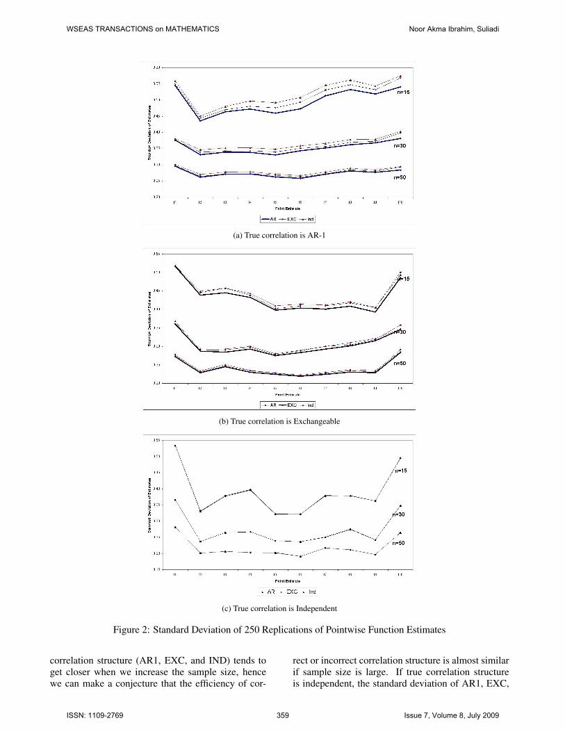
We used standard deviation of 250 replication ateach point estimates to study the consistency and ef-ficiency. The estimator is consistent if standard devi-ation tends to zero when sample size is infinity, i.e.standard deviation decreases while sample size in-creases. This standard deviation can also be used tostudy the efficiency, that is small standard deviationindicates the efficiency of the estimator. Figure 2 andTable 1 show the standard deviation of 250 pointwisefunction estimates.

From Figure 2 and Table 1 we can see the con-sistency of the estimator. The pattern of standard de-viation for all true correlation structures is the same.It decreases when sample size increases. The samepattern is also observed for all correlation structures,using correct or incorect correlation structure. Thismeans that the estimators are consistent and the con-sistency still holds even if we use incorrect correlationstructure. The rate of the decreasing of standard devi-ation from n = 15 to n = 30, and from n = 30 ton = 50, are the same for all true correlation struc-tures. This indicates the convergency rate is (almost)the same for all conditions of true correlation struc-tures. From the standard deviation we can also studythe efficiency of the estimator. From the result of theefficiency study we may conclude whether we need totake into account the correlation into the model or justignore the dependency. The method that has smallervariance or standard deviaton of estimator is more ef-ficient than others.

(a) True correlation is AR-1

(b) True correlation is Exchangeable

(c) True correlation is Independent

Figure 1: Sum of Absolute Deviation of the Three ofTrue Correlation Structures

Figure 2 and Table 1 show that if data are corre-lated (true correlation is autoregressive or exchange-able), for specific sample size, the biggest standarddeviation is obtained if one assumes that the data areindependent. Whilst using true correlation structure,the standard deviation is the smallest. This means thattaking into account the dependency into the model isbetter than assuming data are independent, even weuse incorrect correlation structure. The most efficientestimate is obtained if we use true correlation struc-ture. The difference between standard deviations of



(a) True correlation is AR-1

(b) True correlation is Exchangeable

(c) True correlation is Independent

Figure 2: Standard Deviation of 250 Replications of Pointwise Function Estimates

correlation structure (AR1, EXC, and IND) tends toget closer when we increase the sample size, hencewe can make a conjecture that the efficiency of cor-

rect or incorrect correlation structure is almost similarif sample size is large. If true correlation structureis independent, the standard deviation of AR1, EXC,



Sample Assuming Estimate PointK Corr. f(t1) f(t2) f(t3) f(t4) f(t5) f(t6) f(t7) f(t8) f(t9) f(t10)

Correlation Structure AR-115 AR1 0.545 0.436 0.464 0.472 0.460 0.474 0.513 0.533 0.519 0.541

EXC 0.549 0.445 0.470 0.481 0.476 0.493 0.531 0.547 0.532 0.568IND 0.559 0.451 0.480 0.497 0.493 0.508 0.545 0.562 0.543 0.575

30 AR1 0.377 0.332 0.339 0.338 0.331 0.343 0.352 0.362 0.368 0.381EXC 0.376 0.339 0.342 0.344 0.340 0.351 0.357 0.370 0.373 0.399IND 0.381 0.347 0.352 0.353 0.349 0.359 0.366 0.378 0.380 0.403

50 AR1 0.296 0.262 0.271 0.273 0.263 0.259 0.271 0.282 0.278 0.284EXC 0.298 0.265 0.272 0.273 0.268 0.262 0.273 0.285 0.280 0.293IND 0.301 0.270 0.278 0.279 0.273 0.267 0.278 0.290 0.284 0.295

Correlation Structure Exchangeable15 AR1 0.517 0.445 0.458 0.439 0.403 0.409 0.410 0.417 0.405 0.501

EXC 0.516 0.439 0.445 0.432 0.398 0.404 0.401 0.409 0.393 0.486IND 0.519 0.449 0.458 0.444 0.410 0.415 0.412 0.420 0.405 0.494

30 AR1 0.368 0.290 0.291 0.297 0.278 0.289 0.301 0.304 0.319 0.358EXC 0.360 0.287 0.285 0.293 0.275 0.283 0.293 0.301 0.315 0.345IND 0.363 0.293 0.293 0.301 0.281 0.289 0.300 0.310 0.322 0.348

50 AR1 0.277 0.231 0.247 0.234 0.227 0.221 0.227 0.234 0.230 0.292EXC 0.272 0.229 0.245 0.229 0.224 0.219 0.225 0.230 0.229 0.283IND 0.275 0.233 0.250 0.235 0.228 0.223 0.229 0.237 0.234 0.286

Correlation Structure Independent15 AR1 0.534 0.332 0.379 0.398 0.323 0.322 0.380 0.378 0.363 0.495

EXC 0.534 0.331 0.377 0.397 0.322 0.322 0.379 0.379 0.363 0.495IND 0.534 0.330 0.377 0.396 0.322 0.322 0.378 0.379 0.363 0.495

30 AR1 0.367 0.237 0.265 0.267 0.240 0.236 0.250 0.274 0.242 0.348EXC 0.366 0.237 0.265 0.267 0.239 0.236 0.251 0.275 0.242 0.348IND 0.366 0.237 0.265 0.267 0.239 0.236 0.251 0.275 0.242 0.348

50 AR1 0.282 0.201 0.206 0.203 0.203 0.191 0.217 0.211 0.197 0.265EXC 0.282 0.201 0.206 0.203 0.202 0.191 0.217 0.212 0.197 0.265IND 0.282 0.201 0.206 0.203 0.202 0.191 0.217 0.212 0.197 0.265

Table 1: Standard Deviation of the Estimate Points of Function for Nonparametric Components

and IND are almost similar, for all sample sizes. Thusin this case, the efficiency of using incorrect corre-lation structures is almost similar to the efficiency ofusing correct correlation structure.

5 Application to Real Data

As an application of the proposed method, we useddata of A5055 Long-Term Viral Dynamic Data. Thedata were generated from AIDS Clinical Trials Group,ACTG 5055 study, which was sponsored by NI-AID/NIH. More details of this clinical study can befound in Acosta et al. [1]. Among the total 44 patientsaccrued in this study, 42 subjects were included in theanalysis; of the remaining two subjects, one was ex-

cluded from the analysis because the some covariateswere not obtained and the other was excluded becausethe phenotype assay could not be completed on thissubject. Detection limit of the viral load (HIV RNAcopies) assay is 50 copies per ml blood. If it is belowdetectable, it is imputed as 25 in the data set. Datawere recoded as

yij ={

1, if RNA < 50 copies per ml blood0, otherwise

The covariate is day after treatment. For depen-dent model, we assumed that the structure of correla-tion is exchangeable. This means that the within sub-ject correlations for different lag-time are the same.

As comparison we did three scenarios: (i)parametric approach; (ii) nonparametric (smoothing



Figure 3: Comparison of the Result: the Parametric Approach, Independent, and Dependent GEE-SmoothingSpline

spline) approach with assumption within subject ob-servations are independent; and (iii) nonparametricapproach with assumption within subject observationsare dependent, using GEE-Smoothing Spline. Weused PROC GENMOD for parametric approach, forsmoothing spline we used PROC GAM in SAS 9.0,and SAS IML for GEE-Smoothing Spline.

Results of Parametric and Nonparametric modelare completely different. GEE-parametric model isηij = −1.9619 + 0.0169day, and correlation coef-ficient is r = 0.2467. The P-value of the intercept andcovariate are less than .0001 respectively. The curveof this model shows that P(y=1) will increase slowlywith respect to the increasing of day.

Result of nonparametric approach is definitelydifferent with parametric ones (see Figure 3). Non-parametric models showed that the relationship ofP (y = 1) and day is almost quadratic. Results ofindependent and dependent assumption are almost thesame. From beginning of the day after treatment untilday ≈ 130, those two curves are similar. The differ-ence between those two assumptions started from thispoint, in which the curve of the dependent assump-tion will decrease faster than independent assumption.Another result is P (y = 1) for dependent assump-tion is higher than independent one. For dependentassumption, the estimate of within subject correlationis 0.2208.

6 Conclusion and Discussion

From section 4, it can be concluded that GEE-smooting spline has better properties than GEE-localpolynomial kernel proposed by Lin & Carroll [9]. Thepointwise estimates of GEE-smoothing are consistent,even we use incorrect correlation structure. The con-vergency rates of consistency for independent data (nocorrelation), moderate correlation, and high correka-tion are the same. If data are correlated, ignoringthis correlation in the model, will give the most inef-ficient estimate. Taking into account the dependencyinto the model is better than ignoring it, even using in-correct correlation structure. If data are independent,the efficiency of using correct or incorrect correlationstructures is almost similar. Hence, since in true sit-uation the correlation is unknown, then it is better toassumme the data are correlated rather than to assumedata are independent . We have shown by simulationthat the estimator of GEE-smoothing spline has goodproperties. As an extension for future research, it isimperative these properties should be shown analiti-cally.

Acknowledgements: This research is supported byScience Fund grant Vote No. 5450434 from Ministryof Science, Technology and Innovation Malaysia.



References:

[1] Acosta, E.P, H. Wu, A. Walawander, J. Eron, C.Pettinelli, S. Yu, D. Neath, E. Ferguson, A. J.Saah, D. R. Kuritzkes, and J. G. Gerber, for theAdult ACTG 5055 Protocol Team, Comparisonof two indinavir/ritonavir regimens in treatment-experienced HIV-infected individuals. Journalof Acquired Immune Deficiency Syndromes, 37,2004, pp1358-1366

[2] Adina, Man Milena, C. Bondor, I. Neagoe,M. Pop, A. Trofor, D. Alexandrescu, and O.Arghir, Prognosis Factors in the Evaluation ofMetastatic Breast Cancer, WSEAS TRANSAC-TIONS on BIOLOGY and MEDICINE, 5, 2008,pp281-292.

[3] Davis, Charles S, Statistical Methods for theAnalysis of Repeated Measurements, Springer-Verlag, New York, USA, 2002.

[4] Gonzalez, Gilberto, Lucas Jodar, Rafael Vil-lanuera, and Fransisco Santonja, Random Mod-eling of Population Dynamics with Uncertainty,WSEAS TRANSACTIONS on BIOLOGY andMEDICINE, 5, 2008, pp34-45.

[5] Green, P. J. and B. W. Silverman, Nonpara-metric Regression and Generalized Linear Mod-els. A Roughness Penalty Approach, Chapman &Hall/CRC, New York, USA, 1994.

[6] Hardin, James W. and Joseph M Hilbe, Gen-eralized Estimating Equations, Chapman &Hall/CRC, Washington DC, USA, 2003.

[7] Leisch, Friedrich, Andreas Weingessel and KurtHornik, On the Generation of Correlated Arti-ficial Binary Data. Working Paper. No 13. SFB.Adaptive Information System and Modeling inEconomics and Management Science, ViennaUniversity of Economics and Business Admin-istration, Austria, 1998.

[8] Liang, K. Y. and S. L. Zeger, LongitudinalData Analysis using Generalized Linear Models,Biometrika, 73, 1986, pp13-22.

[9] Lin, Xihong and Raymond J. Carroll, Nonpara-metric Function Estimation for Clustered DataWhen the Predictor is Measured Without/WithError, Journal of the American Statistical Asso-ciation, 95, 2000, pp520-534.

[10] Lin, Xihong and Raymond J. Carroll, Semi-parametric Regression for Clustered Data UsingGeneralized Estimating Equations, Journal ofthe American Statistical Association, 96, 2001,pp1045-1056.

[11] McCullagh, P. and J. A. Nelder, GeneralizedLinear Models 2nd Edition Chapman and Hall,London, UK, 1989.

[12] Raimundo,Silvia Martorano and Ezio Venturino,Drug Resistants Impact on Tuberculosis Trans-mission, WSEAS TRANSACTIONS on BIOL-OGY and BIOMEDICINE, 5, 2008, pp85-95.

[13] Zeger, Scott L. and Kung-Yee Liang, Longitudi-nal Data Analysis for Discrete and ContinuousOutcomes, Biometrics, 42, 1986, pp121-130.

[14] Weddernburn, R. W. M, Quasi-likelihood Func-tions, Generalized Linear Models, and theGauss-Newton Method, Biometrika, 61, 1974,pp439-447.

[15] Welsh, Alan H., Xihong Lin, and Raymond J.Carroll, Marginal Longitudinal NonparametricRegression: Locality and Effeciency of Splineand Kernel Methods. Journal of the AmericanStatistical Association, 97, 2002, 482-493.

[16] Wu, Hulin and Jin-Ting Zhang, Nonparamet-ric Regression Methods for Longitudinal DataAnalysis, John Wiley & Sons, New Jersey, USA,2006.



nonparametric regression for correlated data - wseas.us

Documents