1

Nonlinear Waves on Collinear Currents with Horizontal Velocity Gradient Alexander V. Babanin 1 , Hwung-Hweng Hwung 2 , Igor Shugan 2 , Aron Roland 3 ,

Andre van der Westhuysen 4,5 , Arun Chawla 4 , Caroline Gautier 5

1Swinburne University of Technology, Melbourne, Australia 2 National Cheng Kung University, Tainan, Taiwan 3Technical University of Darmstadt, Germany 4 UCAR Visiting Scientist at NOAA/NWS/NCEP, Camp Springs, MD, USA 5Deltares, Delft, The Netherlands Abstract. Analytical and experimental research of wave dynamics on adverse and following currents with horizontal-velocity gradient, was conducted. Laboratory tests were carried out at the Tainan Hydraulics Laboratory of the National Cheng Kung University of Taiwan, where a special setup aimed at accelerating/decelerating currents was designed, constructed and employed. In the case of accelerating adverse currents, the wave behaviour is strongly nonlinear and leads to downshifting of the wave energy which allows the waves to penetrate the blocking current. For the case of decelerating currents, linear behaviour should lead to amplification of wave amplitude and increase in steepness, which is indeed observed, but downshifting also happens if the initial waves are steep enough. Such results point out to the physics which is presently not accounted for in wave forecast models.

I. Introduction Propagation of waves through spatially and temporally variable currents is a frequent occurrence in coastal areas. In Figure 1, maps of Port Phillip Bay in Australia and Wadden Sea in The Netherlands are shown. Port Phillip (left) is large enough to have its own wind-generated wave system, but it is also open to the Southern Ocean waves, largest on the planet. This is, however, a narrow 1km-wide opening dominated by alternating tidal currents up to a few m/s strong. The Wadden Sea (right) is separated from the North Sea by a chain of barrier islands and the waves – influenced by strong tidal currents - are a combination of penetrated swell and local wind sea.

Figure 1. Maps of Port Phillip (left) and Wadden Sea (right). For Wadden Sea, depth is colour coded according to scale on the right

2

Wave forecast in Port Phillip, Wadden Sea and thousands of similar locations round the world is of great practical significance, as well as for large-scale open-ocean currents with horizontal gradients, for remote sensing applications (e.g. Young et al., 1985, The WISE Group, 2007). Interpretation of the waves on currents, however, is mostly concentrated on the linear and quasi-linear Doppler-shift related or refraction related effects, and even then a large portion of attention has been paid to waves travelling on adverse currents and specifically to the conditions of wave-energy blocking (Chawla and Kirby, 2002, Suastika, 2004, Ardhuin et al., 2007 and references in these papers). These will be briefly reviewed in Section I.1 below. In this paper, we will be specifically interested in what happens to the waves on the opposing currents which do allow penetration of these waves onto the current (Sections II and IV). In the meantime, it is now understood than nonlinear effects may be important. Janssen and Herbers (2009) investigated linear focusing of directional waves on currents which then leads to nonlinear dynamics. Onorato et al. (2011) showed how opposing currents can instigate modulational instability in wave trains. Both studies concentrated on consequences of such nonlinear dynamics for enhancing the probability of freak waves, but the same consequences apply to the probability of wave breaking and hence enhancing the whitecapping dissipation. The topic of fully nonlinear effects will be outlined in Introduction Section 1.2, and in the paper we will again demonstrate significance of these effects and investigate them qualitatively and quantitatively in Sections III and IV. Another topic, largely overlooked previously and highlighted in Section I.3 of Introduction and Section IV of laboratory investigations of the current paper is the waves on decelerating following current. Even in linear sense such waves are to grow steeper, and if so to break more frequently (e.g. Babanin et al., 2007, 2010). Change of the wave breaking rates does not have to be as dramatic as 100% breaking at wave blocking, in order to alter the wave energy dissipation significantly. Typical breaking rates in the ocean are of the order of 2-5% (e.g. Babanin et al. 2001), and therefore an increase of breaking occurrence by a few percent may double the dissipation.

I.1 Wave Blocking Wave blocking is the phenomenon in which waves propagating against an adverse current are stopped. As waves propagate into adverse currents, their group velocity reduces, and at the point of blocking goes to zero. As waves approach this blocking point, they steepen significantly and in most cases there is significant wave breaking. The phenomenon of wave blocking has been known for quite some time (Evans, 1955 conducted experimental studies on using hydraulic breakwaters for stopping waves), however the dynamics of wave blocking are much more complex. Fundamentally, the dynamics of wave current interaction became much clearer with the development of the concept of radiation stresses (Longuet–Higgins and Stewart, 1960, 1961) and the conservation of wave action (Bretherton and Garret, 1969). The latter concept is the fundamental building block for wind wave models. However, these two approaches rely on ray theory, which lead to singularities at the blocking point.

3

Using perturbation stream functions and conducting a local analysis in the neighbourhood of the blocking region, Peregrine (1976) showed that the waves at the blocking point are large but have a finite steepness and are not singular. Smith (1975) developed a uniform asymptotic solution for small waves through the blocking point and showed that if the initial waves are small enough then the waves are reflected at the blocking point with the action flux of the incident and reflected waves being equal and opposite. These reflected waves have a positive phase speed (against the current) but a negative group velocity. As these reflected waves propagate back, they become smaller and smaller till the effects of capillary waves start becoming important (Shyu and Phillips, 1990, Trulsen and Mei, 1993). Some of these processes have been documented in the short-wave experiments of Badulin et al. (1983). This theory has been extended further to include the effects of wave dissipation (Suastika, 2004, Suastika and Battjes, 2009). The limitations of these models are the linear wave assumptions, and they are not easily applicable to practical conditions where there are significant nonlinear processes and frequent wave breaking close to the blocking region. Experimental studies have shown that except for the smallest wave conditions where you have wave blocking with reflection (Chawla, 2000, Suastika 2004), in almost all other conditions there is significant wave steepening and breaking close to the blocking point. Nonlinear processes such as the growth of sideband instabilities is enhanced in the presence of adverse wave currents (Lai et al 1989, Chawla and Kirby 2002, see also Section I.2 below). This coupled with the slowing of the wave group speed have a significant impact on the phenomenon of wave blocking and the evolution of the wave spectra (Chawla and Kirby, 2002). With the enhanced wave steepness close to the blocking region, nonlinear corrections to the dispersion relation play an important role in wave blocking (Chawla and Kirby, 2002). Reproducing these physical processes in wave models is still a significant challenge. There is also very limited data available to adequately quantify energy dissipation due to current-induced breaking close to the blocking region. I.2 Fully Nonlinear Effects of Waves on Currents Traditional research of waves on currents does take into account nonlinear corrections due to finite amplitudes of Stokes waves (see e.g. Chawla and Kirby, 2002, Saustika, 2004 for analyses and further references). Fully nonlinear behaviours, however, such as those which lead to modulational instability, give an additional perspective to wave dynamics on the currents. Janssen and Herbers (2009) studied a combined effect of refraction and nonlinearity of waves with a directional distribution, entering an opposing shearing current. While refraction of such waves can be treated as a largely linear process, it can bring about focusing of the waves. Thus waves become steeper, and if they remain narrow-banded, modulational instability can be triggered or at least enhanced similarly to that observed in directional wave fields without current by Babanin et al. (2011). Janssen and Herbers (2009) point out an increased probability of freak waves, but in the context of wave modelling which is the target of this paper, such instability should cause enhanced breaking and spectrum-energy downshifting, the latter was indeed observed by Janssen and Herbers (2009).

4

Onorato et al. (2011) specifically studied modulational instability triggered in a stable unidirectional wave train when entering an adverse current. They used a modified Nonlinear Shroedinger Equation of Hjelmervik and Trulsen (2009), which modification allows for a current, provided its magnitude is small compared with wave phase velocity. That is, the conditions are far from the wave-blocking limit and let the waves propagate onto the current. Such wave trains exhibit modulational instability whose magnitude depends on the ratio of the current velocity and wave group velocity. If the initial one-dimensional wave field is random, modulational instability is also enhanced by the presence of the current gradient. Again, the authors were mostly interested in probability of freak waves, but in the wave-modelling perspective these results should be interpreted as an increased probability of wave breaking and hence an enhanced whitecapping dissipation. Another possible aspect of nonlinear behaviour in wave-current system should also be mentioned, this is nonlinear exchanges by energy between the waves and the currents. Although for currents, such exchanges are apparently negligible, for waves this may potentially indicate an essential drop or gain of energy, and consequently decrease or increase of wave steepness which is connected with the breaking probability (Babanin et al. 2007, 2011). Such alterations of the steepness would then lead to variations of the whitecapping dissipation of waves propagating over the current, as well as to changes to the wave spectrum through non-breaking nonlinear effects such as spectral-energy downshifting which is frequently observed in experiments described in this paper. I.3. Van der Westhuysen Wave-Current Dissipation Van der Westhuysen (2011) presents a semi-empirical expression for the enhanced dissipation of essentially linear waves on current gradients. This expression was introduced since the linear action balance equation of SWAN displayed strong overestimation of significant wave heights in both the far field (away from the blocking point) and the near field (at the blocking point) in partially and fully blocking wave-current interaction flume experiments. The proposed dissipation term is based on the saturation-based whitecapping expression of Van der Westhuysen et al. (2007). Wind waves in the field experience steepening, and subsequently breaking, due to various processes, including energy transfer from wind, shoaling due to bathymetry and shoaling due to gradients in the ambient current. In order to isolate the contribution of current gradients in the increased steepness and resulting dissipation, Van der Westhuysen (2011) proposes to scale the degree of whitecapping dissipation with the incremental shortening/steepening of the waves due to negative current gradients, which is related to the relative Doppler shifting rate cσ/σ. The formulation reads:

( )2( , ) ( ), max ,0 ( , )

p

ds dsr

c B kS C EB

σ σ θσ θ σ θ

σ⎡ ⎤⎡ ⎤

= − ⎢ ⎥⎢ ⎥⎣ ⎦ ⎣ ⎦ , (1)

where σ is the intrinsic (relative) radian frequency, θ is the mean wave direction and E the variance density spectrum. From linear theory, the propagation in frequency space cσ is given by (e.g. Mei, 1983):

5

gd d Uc U d c kdt d t sσ

σ σ∂ ∂ ∂⎡ ⎤= = + ⋅∇ − ⋅⎢ ⎥∂ ∂ ∂⎣ ⎦

rrr, (2)

in which s is the space coordinate in the propagation direction θ, d is the water depth, cg the wave group velocity, k

r the wavenumber vector and U

r the current velocity

vector. The last term on the right-hand side of (2) is considered to be dominant in practical cases such as the tidal inlets of the Dutch Wadden Sea. The calibration coefficient Cds = 0.8 in (1) was found from calibration to laboratory data. A maximum function is included in order to take only relative increases in steepness into account in the enhanced dissipation. The formulation (1) is applied as an additional dissipation term in the action balance equation. Note that negative current gradients occur both for accelerating opposing currents and decelerating following currents, both of which result in steepening of the waves, as will be shown below. The remaining parameters are as defined and calibrated in Van der Westhuysen et al. (2007): B(k) is the spectral saturation and Br is a threshold saturation level, which has been calibrated to Br = 1.75×10-3. The parameter p is a function of the inverse wave age u*/c, based on scaling arguments involving a spectral balance between the wind input, whitecapping and nonlinear interaction terms.

II. Stokes Waves in Presence of Current Here, we will conduct a theoretical analysis of the nonlinear Stokes surface wave propagation in the presence of a non-uniform long-scale horizontal current ( )U U x= where x is the horizontal coordinate. The analysis will be based on the set of modulation equations derived by Hwung et al. (2009):

- dispersion relation for nonlinear surface waves on deep water:

2 4 2 20 0 0 0 0( 2 ) /tt xt xxgk k U Uσ φ φ φ φ φ= + + + + , (3)

- wave action conservation law in the presence of current:

2 20 0[ ] [( ) ] 0

2t xgUφ σ φ σσ

+ + = , (4)

- condition of wave phase compatibility:

( ) 0t xk kUσ+ + = , (5)

where ( , )k σ - wavenumber and intrinsic frequency of waves, correspondingly; 0φ is the amplitude of the velocity potential, g is the gravity acceleration and t is time.

6

The stationary model of interaction gives the conservation of wave action flux 0A and a constant value for the absolute frequency of waves 0Ω at any space point x, following from (4) and (5), correspondingly:

20 0( )

2gU Aφ σσ

+ = ; (6)

0kUσ + =Ω . (7)

So, for a stationary regime of interaction, the wavenumber k and the intrinsic frequency σ will change in accordance with the variability of the current due to (7); the wave action flux 0A and observable wave frequency 0Ω will be constant for all x. After eliminating wavenumber k and frequency σ , the set of equations (3), (6) and (7) transforms into a single equation for the first-order potential amplitude 0φ :

422 20 0 0 00 0 02 2 2 2 2

0 0

( 4 )1 1 /4 2 xx

A g g U Ag UU U U U

φ φ φφ φ

⎛ ⎞⎛ ⎞ ⎛ ⎞+ Ω Ω= + − + +⎜ ⎟⎜ ⎟ ⎜ ⎟⎜ ⎟⎝ ⎠ ⎝ ⎠⎝ ⎠

. (8)

The last two terms on the right of (8) represent the higher-order nonlinear amplitude Stokes correction and the effect of amplitude dispersion, respectively. It has to be mentioned that neglecting these two terms gives the main singularity of the linear regime of the modulation – solution of the equation (8) does not exist for strong enough adverse current:

04gU < −Ω

. (9)

Eq. (9) exactly expresses the blocking phenomenon of surface waves by adverse current – wave amplitude in the vicinity of blocking point will tend to infinity. For example, waves with period T=1 Sec will be blocked by a current of U ~ 0.4 m/sec. The linear modulation solution is not valid in such a regime, and taking account of the higher order dispersion properties in the equation (8) is necessary. Let us consider results of simulations for wave propagation, based on the equation (8) for conditions of laboratory experiments described below, and compare it to the linear solutions. The horizontal current profile ( )U U x= will be taken in the following parametric analytical form:

( ){ }0 1 1 2[ ( 75)] [ (105 )] / 2U U Tanh U x Tanh U x U= − + − + , (8)

where 2U is magnitude of the generated current, 0U is value of the current change due to elevation of the bottom level in Figure 6, and 1U characterizes the gradient of bottom variability. An example of the current profile for typical laboratory conditions ( )2 0 10.2 / sec, 0.2 / sec, 0.6 1/U m U m U m= − = − = is presented in Figure 2.

7

Figure 2. Example of a current profile Let us compare results of the simulations for the linear and nonlinear models of wave-current interaction, for different magnitudes of the adverse current. An example of a non-blocking regime of interaction with initial wave period T=1sec, height of generated waves H=2a=0.05m and current speed parameters ( )2 0 10.1 / sec, 0.1 / sec, 0.6 1/U m U m U m= − = − = is presented at Figure 3(a)-3(c). That is, maximal opposing current speed is 0.2 / secmU m= − .

Figure 3(a). Wave amplitude modulation for the linear (L) and nonlinear models (NL). 0.2 / secmU m= −

8

Figure 3(b). Wavenumber modulation for the linear (L) and nonlinear models (NL).

0.2 / secmU m= −

Figure 3(c). Wave steepness modulation for the linear (L) and nonlinear models (NL).

0.2 / secmU m= − One can see that difference in the results between these two models, for the regimes which are relatively far from the wave blocking condition (9), is quite small and linear model performs reasonably well. Results of calculations for a near-blocking regime of

9

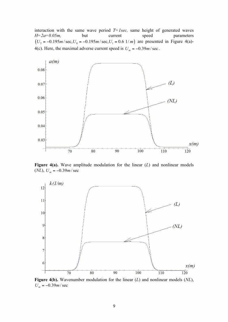
interaction with the same wave period T=1sec, same height of generated waves H=2a=0.05m, but current speed parameters ( )2 0 10.195 / sec, 0.195 / sec, 0.6 1/U m U m U m= − = − = are presented in Figure 4(a)-4(c). Here, the maximal adverse current speed is 0.39 / secmU m= − .

Figure 4(a). Wave amplitude modulation for the linear (L) and nonlinear models (NL), 0.39 / secmU m= −

Figure 4(b). Wavenumber modulation for the linear (L) and nonlinear models (NL),

0.39 / secmU m= −

10

Figure 4(c). Wave steepness modulation for the linear (L) and nonlinear models (NL),

0.39 / secmU m= − The linear modulation model in the near-blocking conditions produces outcomes which exhibit very large differences with respect to the higher-order nonlinear model. The principal difference here is that the wave steepness in the linear model exceeds more than two times the Stokes wave limiting steepness which signifies wave-breaking threshold for one-dimensional waves (Babanin et al., 2007), while the nonlinear model does not reach this threshold. Finally, the results for a wave blocking regime of interaction, with the same wave period T=1 sec, same height of generated waves H=2a=0.05m, and current speed parameters of ( )2 0 10.2 / sec, 0.2 / sec, 0.6 1/U m U m U m= − = − = are shown in Figure 5(a) -5(c). Now the maximal adverse current speed is 0.4 / secmU m= − .

11

Figure 5(a). Wave amplitude modulation for the linear (L) and nonlinear models (NL), 0.4 / secmU m= − .

Figure 5(b). Wavenumber modulation for the linear (L) and nonlinear models (NL),

0.4 / secmU m= − .

12

Figure 5(c). Wave steepness modulation for the linear (L) and nonlinear models (NL),

0.4 / secmU m= − . The linear model of interaction totally fails under these blocking conditions, while the nonlinear model still works and gives modulations of wave steepness under the breaking threshold. The waves in the presented nonlinear model propagate through the linear-blocking region, they are rather steep and will break soon (see Babanin 2007, 2010). For very strong adverse currents, even the nonlinear model will lead to wave steepness exceeding the wave breaking limit, and so the region of applicability for such a model have to be investigated additionally.

III. Laboratory Facility and the Experiment Laboratory tests were carried out at the Tainan Hydraulics Laboratory of the National Cheng Kung University of Taiwan, where a special setup aimed at accelerating/decelerating currents was designed, constructed and employed. The tank is 200m long, with a wavemaker on one end and pumps arranged in such a way that they can generate currents in both adverse and following directions. In Figure 6 (top), the general setup of the experiment is shown, and below that the geometry of the bottom elevation and arrangement of the wave probes around this elevation are detailed. A vertical array of current meters was deployed in the centre of the bottom elevation. In the table, WH are wave probes and EMC are current meters. In the tank, probes 1 and 2, and probes 5 and 6 are located in close proximity for intentional redundancy. In the analysis of Section IV below, each of these two pairs will be treated as a single probe, and distant probe 12 will not be employed. So in the experimental figures the probe numbering will be changed as described in the beginning of Section IV. As seen in Figure 6, waves are generated in the still water, and then enter the current above the pump opening at the bottom of the tank where

13

they may undergo some aritificial transformations. Therefore, features of this transition of the waves should be interpreted with caution.

wave maker

Motor Driver

Interface

Control program

wave making machine control system

wave absorb

section

observation window

MNDAS

73m 4m 6m

2m

2m

wave gauge

data acquisition system

The image cannot be displayed. Your computer may

78m 39m

load cell structure

contra-propeller

pipeline

1 2 3 5 6 7

8 9

10 11 12 4

83.9 123.1 196 6.0 0.0

Figure 6. Top: General setup of the laboratory tank and wave-current experiment. Bottom: Detailed arrangement of the wave probes and current meters around the bottom elevation in the centre of the tank.

14

IV. Laboratory Experiment with Adverse Current

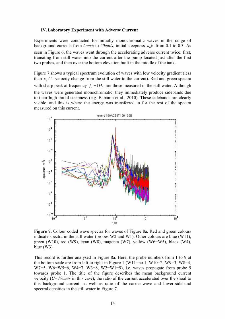
Experiments were conducted for initially monochromatic waves in the range of background currents from 6cm/s to 20cm/s, initial steepness a0k from 0.1 to 0.3. As seen in Figure 6, the waves went through the accelerating adverse current twice: first, transiting from still water into the current after the pump located just after the first two probes, and then over the bottom elevation built in the middle of the tank. Figure 7 shows a typical spectrum evolution of waves with low velocity gradient (less than cg / 4 velocity change from the still water to the current). Red and green spectra with sharp peak at frequency fp =1Hz are those measured in the still water. Although the waves were generated monochromatic, they immediately produce sidebands due to their high initial steepness (e.g. Babanin et al., 2010). These sidebands are clearly visible, and this is where the energy was transferred to for the rest of the spectra measured on this current.

Figure 7. Colour coded wave spectra for waves of Figure 8a. Red and green colours indicate spectra in the still water (probes W2 and W1). Other colours are blue (W11), green (W10), red (W9), cyan (W8), magenta (W7), yellow (W6=W5), black (W4), blue (W3)

This record is further analysed in Figure 8a. Here, the probe numbers from 1 to 9 at the bottom scale are from left to right in Figure 1 (W11=no.1, W10=2, W9=3, W8=4, W7=5, W6=W5=6, W4=7, W3=8, W2=W1=9), i.e. waves propagate from probe 9 towards probe 1. The title of the figure describes the mean background current velocity (U=19cm/s in this case), the ratio of the current accelerated over the shoal to this background current, as well as ratio of the carrier-wave and lower-sideband spectral densities in the still water in Figure 7.

15

In the top panel, asterisks indicate frequency of the spectrum peak at each location along the tank. The dotted black line shows the position where the lower sideband was located in still water (probe no. 9), and this is exactly where the peak frequency is measured by the stationary probes positioned along the current (8 through 1). Therefore, the current stimulates downshifting of wave energy to the lower sideband which appears to be irreversible. The middle subplot demonstrates measured wave-amplitude evolution defined as a = 2 ! std(e) where e is time series of the surface elevations. Amplitude rapidly drops between probes 9 and 8, i.e. between the still water and waves on the current. Distance between these probes is about 60m, but the measured friction against the wall is very small, therefore the energy drop should be attributed to the wave breaking. Initial steepness of the waves is quite high (ak=0.15 in the still water), and such waves would break within some 30 wavelength even without the current (Babanin et al., 2007). Further evolution of the wave amplitude is apparently induced by the current: the amplitude grows between probes 8 and 6 (where the adverse current accelerates) and then reduces (current decelerates). The bottom subplot requires special attention. This is the evolution of the wave steepness ak over the current. Asterisks indicate steepness of waves of amplitude a for the variable wavenumber k of waves with frequency fp =1Hz in the still water. These waves, however, as we see from the top subplot, are no longer the peak, and steepness in terms of wavenumber of the actual peak waves on the current is shown with circles. This steepness is lower and such waves penetrate the current without breaking, even if the original peak frequency is blocked by the adverse current as we will see below.

16

Figure 8. Arranged in three subplots, three cases of wave propagation through the tank, (a) – top, (b) – middle, (c) – bottom. In each case, top subplot is peak frequency, middle panel is wave amplitude, bottom subplot is wave steepness for the original

17

frequency (asterisks) and measured peak frequency (circles). Background current speed is shown in the title of the top subplot in each case

Another example, with much smaller current velocity of U=6cm/s, is shown in Figure 8b. The behaviour of the frequency downshift is the same, as is that for the wave amplitude evolution and steepness. A similar pattern is observed in Figure 8c with U=13cm/s.

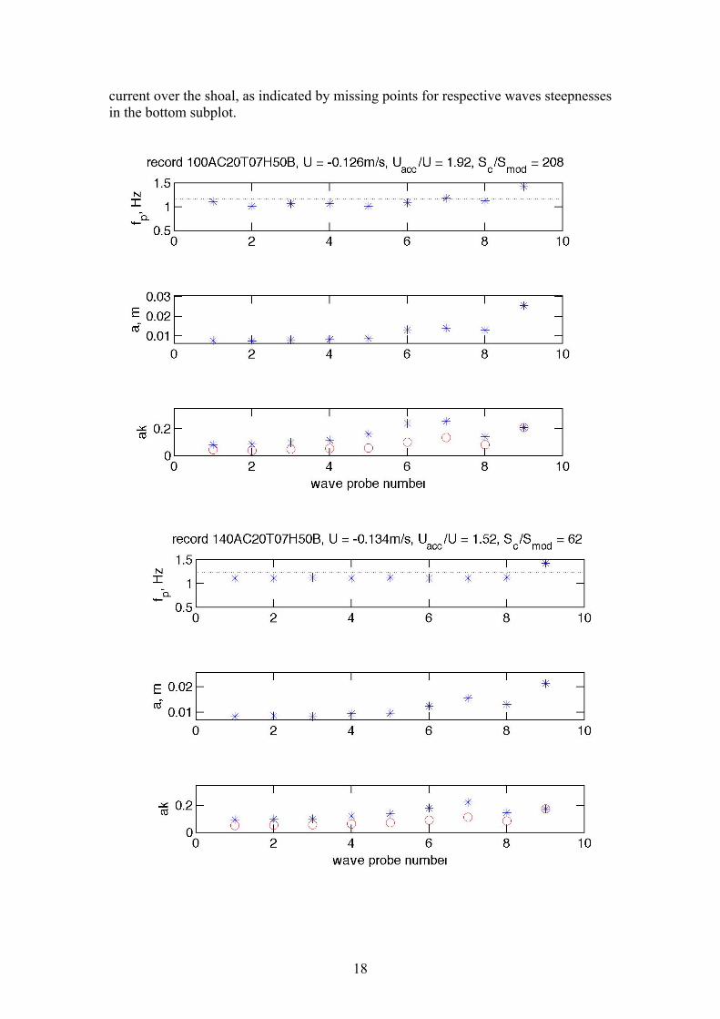
Substantially different is downshifting of wave energy in cases of stronger velocity gradients (here, we conventionally separated the second group of cases as those with the initial velocity change greater than cg / 4 ). For fp =1.4Hz on U=12cm/s, the progression of spectra in Figure 9 shows a gradual decrease of the peak frequency.

Figure 9. Colour coded wave spectra for waves of Figure 10a. Red and green colours indicate spectra in the still water (see caption of Figure 7) Figure 10a depicts the spectra shown in Figure 9. It is clear that initially waves corresponding to the lower sideband are produced (as seen in Figure 8), but eventually they evolve into essentially longer waves. This again points to the role of current gradients in the irreversible downshifting of the wave energy. Patterns for the wave amplitude and steepness are similar to Figure 8, but the initial drop of the amplitude is more significant. For the same initial frequency fp =1.4Hz , approximately same initial amplitude, but stronger currents, the downshifting evolves rapidly to frequencies lower than the initial lower sideband (Figures 10b and 10c). Most informative is Figure 10c, where both the initial peak frequency and the initial lower sideband are blocked by the

18

current over the shoal, as indicated by missing points for respective waves steepnesses in the bottom subplot.

19

Figure 10. Arranged in three subplots, three cases of wave propagation through the tank, (a) – top, (b) – middle, (c) – bottom. In each case, top subplot is peak frequency, middle panel is wave amplitude, bottom subplot is wave steepness for the original frequency (asterisks) and measured peak frequency (circles). Background current speed is shown in the title of the top subplot in each case. Missing points in the bottom subplot indicate wave blocking

V. Laboratory Experiment with Following Current

The dynamics of waves on following current, observed in the laboratory experiment, are determined by the combination of linear and nonlinear effects. If the initial steepness of waves in still water is small, sidebands are absent and waves are strictly monochromatic, the same narrow single peak is maintained throughout (Figure 11). The evolution of such a wave train over the following current is depicted in Figure 12, using the same notation as above for the adverse current (again, waves propagate from right to left). The peak frequency in the top subplot remains unchanged. The middle subplot confirms expectations of the linear theory. Acceleration starts at probe 8 and causes reduction of wave amplitude, and deceleration begins after probe 5 and brings about wave growth. The pattern of wave steepness on the current repeats the trend of the wave amplitude (bottom panel). Probes 9 and 1 are distant and indicate some additional dynamics due to transition from the still water to the current between probes 9 and 8 over the pump opening at the bottom and non-uniform transient vertical current distribution at this place, and perhaps due to breaking between probes 2 and 1.

20

Figure 11. Colour coded wave spectra for waves of Figure 12. Red and green colours indicate spectra in the still water (see caption of Figure 7)

Figure 12. Wave propagation through the tank. Top subplot is peak frequency, middle panel is wave amplitude, bottom subplot is wave steepness for the original

21

frequency (asterisks) and measured peak frequency (circles). Background current speed is shown in the title of the top subplot in each case In Figure 13, spectra of much steeper initial waves are shown. Immediately, they exhibit sidebands (red spectrum), and the lower sideband then grows into the main peak (blue spectrum).

Figure 13. Colour coded wave spectra for waves of Figure 14. Red and green colours indicate spectra in the still water (see caption of Figure 7) The evolution of such a wave train is illustrated in Figure 14. The wave amplitude (middle panel) retains the same pattern as in Figure 12 for linear waves. Different only is the amplitude on probe 9 in the still water, which corresponds to a large initial steepness in the bottom subplot and should have led to breaking before waves reach probe 8. The pattern of the wave steepness (bottom panel) is smeared because the spectrum broadens and the peak frequency in the upper panel moves to the lower sideband according to Figure 13.

22

Figure 14. Wave propagation through the tank. Top subplot is peak frequency, middle panel is wave amplitude, bottom subplot is wave steepness for the original frequency (asterisks) and measured peak frequency (circles). Background current speed is shown in the title of the top subplot in each case

VI. Conclusions Analytical and experimental research of wave dynamics on currents with horizontal-velocity gradient, was conducted. Nonlinear effects appear to be very significant. Theoretical investigation of Stokes waves on adverse currents demonstrates that when the linear wave theory fails into a singularity while current speeds approach wave-blocking magnitudes, the nonlinear theory performs realistically. At the blocking point it leads to steepness close to the Stokes limiting steepness which also indicates the wave breaking threshold. That is, the waves will be breaking soon, as does happen in the experiment, but there are no unlimited steepness predictions. In laboratory tests, however, it is apparent that fully nonlinear behaviours are essential for waves on currents. In the experiments, a special setup aimed at accelerating/decelerating the currents was employed. In case of the accelerating adverse currents, the wave behaviour is strongly nonlinear and leads to downshifting of the wave energy which allows the waves even to penetrate the blocking current. For the case of decelerating folowing currents, linear behaviour should lead to amplification of wave amplitude and an increase in steepness, which is indeed observed, but downshifting also happens if the initial waves are steep enough. Such results point out to the physics which is presently not accounted for in wave forecast models. This is an important application to be conducted, as waves entering

23

currents with horizontal gradients are a frequent occurrence in the ocean, and particularly in coastal areas with tidal inlets and channels.

References

Ardhuin, F., K. Belibassakis, I.V. Lavrenov, R. Magne, H.L. Tolman, 2007: Wave propagation. Progress in Oceanography, 75, 622-632 (In Wave modeling – the state of the art by The WISE Group (Cavaleri, L., J.-H.G.M. Alves, F. Ardhuin, A. Babanin, M. Banner, K. Belibassakis, M. Benoit, M. Donelan, J. Groeneweg, T.H.C. Herbers, P. Hwang, P.A.E.M. Janssen, T. Janssen, I.V. Lavrenov, R. Magne, J. Monbaliu, M. Onorato, V. Polnikov, D. Resio, W.E. Rogers, A. Sheremet, J. McKee Smith, H.L. Tolman, G. van Vledder, J. Wolf, and I. Young), Progr. Oceanogr., 75, 603-674) Babanin, A.V., I.R. Young, and M.L. Banner, 2001: Breaking probabilities for dominant surface waves on water of finite constant depth. J. Geophys. Res., C106, 11659-11676 Babanin, A.V., D. Chalikov, I.R. Young, and I. Savelyev, 2007: Predicting the breaking onset of surface water waves. Geophys. Res. Lett., 34, L07605, doi:10.1029/2006GL029135, 6p Babanin, A.V., D. Chalikov, I.R. Young, and I. Savelyev, 2010: Numerical and laboratory investigation of breaking of steep two-dimensional waves in deep water. J. Fluid Mech., 644, 433-463 Badulin, S.I., K.V. Pokzayev, A.D. and Rosenberg, 1983: A laboratory study of the transformation of regular gravity – capillary waves in inhomogenous flows. Izv. Atmos. Ocean. Phys.,19, 782-787 Bretherton, F.P., and C.J.R. Garett, 1969: Wavetrains in inhomogenous moving media. Proc. Roy. Soc. London A., 302, 529–554 Chawla, A., 2000: An experimental study on the dynamics of wave blocking and breaking on opposing currents. Ph D. Thesis, University of Delaware, Newark, DE, 174p Chawla, A., and J.T. Kirby, 2002: Monochromatic and random wave breaking at blocking points. J. Geophys. Res., C107, 3067, 10.1029/2011JC001042, 19p Evans, J. T., 1955: Pneumatic and similar breakwaters. Proc. Roy. Soc. London, A231, 457–466 Hjelmervik, K.B., and K. Trulsen, 2009: Freak wave statistics on collinear currents. J. Fluid Mech., 637, 267-284 Hwung, H.-H., R.-Y. Yang, and I. Shugan, 2009: Exposure of internal waves on the sea surface. J. Fluid Mech., 626, 1-20 Janssen, T.T. and T.H.C Herbers, 2009: Nonlinear wave statistics in a focal zone. J. Phys. Oceanogr., 39, 863-884 Lai, R. J., S.R. Long, and N.E. Huang, N.E., 1989: Laboratory studies of wave-current interaction: kinematics of the strong interaction. J. Geophys. Res., 94, 16201–16214 Longuet–Higgins, M. S., and R.W. Stewart, 1960: Changes in the form of short gravity waves on long waves and tidal currents. J Fluid Mech., 8, 565–583

24

Longuet–Higgins, M. S., and R.W. Stewart, 1961: The change in the amplitude of short gravity waves on steady non-uniform currents. J Fluid Mech., 10, 529–549 Mei, C. C., 1983: The applied dynamics of ocean surface waves. Wiley, New York, 740p Onorato, M., D. Proment, and A. Toffoli, 2011: Triggering rogue waves in opposing currents. Phys. Rew. Lett., in press Peregrine, D. H., 1976: Interaction of water waves and currents. Advances in Appl. Mech., 16, 9–117 Saustika, I.K., 2004: Wave blocking. PhD Thesis, Technische Universiteit Delft, 157p Suastika, I.K., and J.A. Battjes, 2009: A model for blocking of periodic waves, Coastal Eng. J., 51, 81–99 Shyu, J. H., and O.M. Phillips, 1990: The blockage of gravity and capillary waves by longer waves and currents. J Fluid Mech., 217, 115–141 Smith, R., 1975: Reflection of short gravity waves on a non-uniform current. Math. Proc. Camb. Phil. Soc., 78, 517–525 Trulsen, K., and C.C. Mei 1993: Double reflection of capillary / gravity waves on a non-uniform current: A boundary layer theory. J Fluid Mech., 251, 239–271 Van der Westhuysen, A. J., 2011: Spectral modeling of wave dissipation on negative current gradients. Coastal Eng., in review Van der Westhuysen, A. J., M. Zijlema, and J. A. Battjes, 2007: Nonlinear saturation-based whitecapping dissipation in SWAN for deep and shallow water. Coastal Eng., 54, 151-170 WISE Group, The (Cavaleri, L., J.-H.G.M. Alves, F. Ardhuin, A. Babanin, M. Banner, K. Belibassakis, M. Benoit, M. Donelan, J. Groeneweg, T.H.C. Herbers, P. Hwang, P.A.E.M. Janssen, T. Janssen, I.V. Lavrenov, R. Magne, J. Monbaliu, M. Onorato, V. Polnikov, D. Resio, W.E. Rogers, A. Sheremet, J. McKee Smith, H.L. Tolman, G. van Vledder, J. Wolf, and I. Young), 2007: Wave modeling – the state of the art. Progr. Oceanogr., 75, 603-674

Young, I.R., W. Rosenthal, and F. Ziemer, 1985: A three-dimensional analysis of marine radar images for the determination of ocean wave directionality and surface currents. J. Geophys. Res., 90, 1049-1060