nonlinear wave transmission and pressure on the fixed ... · 52 m. ghiasi et al./ nonlinear wave...

11(2014) 051 - 074

Abstract Fully nonlinear wave interaction with a fixed breakwater is inves-tigated in a numerical wave tank (NWT). The potential theory and high-order boundary element method are used to solve the boundary value problem. Time domain simulation by a mixed Eulerian-Lagrangian (MEL) formulation and high-order boundary integral method based on non uniform rational B-spline (NURBS) formulation is employed to solve the equations. At each time step, Laplace equation is solved in Eulerian frame and fully non-linear free-surface conditions are updated in Lagrangian manner through material node approach and fourth order Runge-Kutta time inte-gration scheme. Incident wave is fed by specifying the normal flux of appropriate wave potential on the fixed inflow boundary. To ensure the open water condition and to reduce the reflected wave energy into the computational domain, two damping zones are provided on both ends of the numerical wave tank. The conver-gence and stability of the presented numerical procedure are ex-amined and compared with the analytical solutions. Wave reflec-tion and transmission of nonlinear waves with different steepness are investigated. Also, the calculation of wave load on the break-water is evaluated by first and second order time derivatives of the potential. Keywords Fully Nonlinear, Numerical Wave Tank, Mixed Eularian-Lagrangian, NURBS, Potential Flow.

Nonlinear wave transmission and pressure on the fixed truncated breakwater using NURBS numerical wave tank

1 INTRODUCTION

In the shallow water, as the wave approaches the shore, its energy gradually increases. Therefore, shore protection is required to keep the shore and to provide the calm water condition. The break-waters are widely used to make progressive wave amplitude fade away. Wave run-up mechanism can result in the loss of wave energy on rear side of the breakwater.The motion of fluid particles on the free surface in front of the breakwater is fully nonlinear.

Arash Abbasn ia

Mahmoud Ghias i *

Department of Maritime Technology, Amir-kabir Universityof Technology, Tehran, Iran, 15875-4413 Received in 18 Nov 2012 In revised form 03 May 2013 * Author email: [email protected]

52 M. Ghiasi et al./ Nonlinear wave transmission and pressure on the fixed truncated breakwater using NURBS numerical wave tank

Latin American Journal of Solids and Structures 11(2014) 051 - 074

In the past three decades, a lot of efforts have been made to develop the computational tools equivalent to a laboratory wave tank facilities. In general, these attempts are categorized into po-tential and viscous NWTs. Most of the works have been focused on developing fully nonlinear wave generation and propagation in both two- and three-dimension inviscid numerical tank. Mixed Eu-lerian-Lagrangian time marching method (MEL) developed by Longuet-Higgins and Cokelet (1976) have been widely used in potential NWTs. In MEL scheme, at each time step, the Laplace equation is solved in the Eulerian frame and the moving boundary points update in a Lagrangian manner. The boundary integral equation can be employed to obtain the velocity potential at each time step in fluid control volume. Then, the time integration of the fully nonlinear free surface boundary con-dition in Lagrangian manner is conducted to evaluate the boundary value and new position of the surface for the next time step.

Inflow boundary condition is implemented by putting wavemaker on upstream of the flow. At NWT, instead of wavemaker, an artificial wave generator is used on the inflow boundary by dis-tributing sources in the fixed vertical wall. The wave characteristics might be defined by the wave theories. Different types of wavemakers have been reviewed in detail by Tanizawa (2000) and Newman (2010).Wave absorber is deployed at upstream and downstream boundaries to prevent wave reflection from end walls. This function is essential to maintain unbounded region condition during a long time simulation and to avoid the nonphysical manner due to the propagation of re-flected wave from the end walls within the computational domain.

The boundary element method is efficientin solving the Laplace equation in free surface flow problems. Indirect boundary element method was used in NWT by Zhang et al. (2006) for modeling the linear and nonlinear wave propagation and the wave shoaling on submerged obstacles. The di-rect method has been widely used based on different formulations in potential NWTs. Constant element formulation, as the simplest one, was employed by Ryu et al. (2003) to simulate current-wave interaction in the 2D NWT. The linear elements approach was used by Buchmann et al. (1998) to predict wave run-up on structure in numerical wave tank and, analogously, this method was treated to determine Bragg reflection in 2D NWT by Tang et al. (2008). Curvilinear element was employed by Baudic et al. (2001) to describe the boundaryin nonlinear potential wave tank.A boundary element formulation based on B-splines is developed by Carbal et al. (1990) for higher degrees of continuity of the geometric boundary and variables. Also, this formulation was extended for lowering the degree of continuity of the variables at points of geometric discontinuity by Carbal et al. (1991).

First order and second order finite difference formulation in time as low order time integration method were employed in NWT by Ryu et al. (2003), Wu &Tsay (2005) and Xiao et al. (2009). High-order time integral methods such as fourth order Runge-Kutta method by Koo (2003), fifth order Runge-Kutta-Gil and fourth order Adams-Bashforth-Moulton method by Zhang et al. (2005) were also used.

Discontinuity in the normal flux occurs on intersection of the free surface and end walls or body hull boundary (corner points). This discontinuity severely affects the stability of the solution. To overcome these difficulties, some remedies were proposed. The double nodes technique is one of the suitable methods. This technique was developed by Grilli et al. (1990). The other one is discontin-

M. Ghiasi et al./ Nonlinear wave transmission and pressure on the fixed truncated break water using NURBS numerical wave tank 53


ues elements recommended by Brebbia and Dominguez (1992). These techniques are compared with each other in standing wave problem by Hamano et al. (2003).

During the free surface simulation of nonlinear waves, the nonphysical saw tooth instability may happen. Instabilities may also occur due to variable mesh size or natural singular treatment at the intersection of wavemaker and free surface. To treat the so-called saw tooth instability, smoothing schemes have been already used such as Chebyshev five-point smoothing scheme by Koo (2004), and the B-spline smoothing scheme.

In the present paper, nonlinear wave interaction with a fixed box-type breakwater is analyzed by a two dimensional fully nonlinear NWT. The NWT is developed based on the potential theory, MEL, and high-order boundary element method by NURBS formulation. Discretizing of the com-plicated free surface boundary and the distribution of the velocity potential over the boundaries is also based on the NURBS approximation.The two artificial damping zones proposed by Cointe (1990) are implemented at the ends of the tank to absorb the reflected wave from the end walls into the computational domain. The wavemaker is treated by an artificial wave generator.

Material node approach scheme is applied as time marching scheme. Also, the tangential deriva-tive of potential on the free surface is accurately obtained by NURBS approximation. The fourth order Runge-Kutta time integration scheme is used to update the free surface boundary value and positions. Kinematics of corner points is calculated by applying double nodes technique. To over-come the nonphysical saw tooth instability, five point Chebyshev smoothing scheme is employed at every several time steps.

Time derivative of potential on the body is estimated numerically by first and second order fi-nite difference formulation to measure wave load on the body. Performance of present numerical procedure is verified by theoretical results. Numerical solutions show that the NURBS NWT can successfully simulate the nonlinear wave body interaction.

2 THEORITICAL DEVELOPMENT

Assume a NWT with length L and a constant depth d and the damping zones located at both ends of the tank. The fixed box-type breakwater is located at the wave tank with the width B and the submergence depth D . A Cartesian coordinate system Oxz( ) with origin O is placed on the

mean water surface with the positive z -axis directed vertically upwards asFigure 1. The fluid is assumed to be homogeneous, incompressible, and inviscid and its motion is irrota-

tional. The governing equation of the velocity potential φ x, z,t( ) is given by Laplace’s equation in

the domain R t( ) .

∇2φ = 0 in R t( ) (1)

The solution must satisfy bottom, free surface, and input and output boundary conditions.



2.1 Boundary and initial conditions

There are two fully nonlinear boundary conditions, kinematic (KFSBC) and dynamic boundary condition (DFSBC) on the free surface ( S f ) as defined by Dean and Dalrymple (1991).

∂η∂x

= ∂φ∂z

− ∂φ∂x

∂η∂x

(KFSBC)

∂φ∂t

= −gz − 12∇φ

2 (DFSBC)

on S f (2)

Both boundary conditions are applied on the exact free surface. η x,t( ) is the wave elevation

measured from still water level. t indicates the time of simulation and g is gravitational accelera-tion.

Figure 1Definition Sketch

Impermeable condition is specified on the breakwater body ( Sh ), rigid bottom boundary ( Sb )

and wall boundary at the end of wave tank ( Sw ).

∂ϕ∂n

= 0 on Sb , Sw and Sh (3)

n is the normal vector directed outward of the control domain. Based on the given incident ve-locity potential function (φwg ), the normal velocity at input boundary ( Si ) is written as:

∂φ∂n

= −∂φwg∂x

on Si (4)

According to Koo and Kim (2004), the nonlinear second order stokes wave is adopted in input

boundary.

d)(tR

Damping

Zone 1

Damping

Zone 2

wS

Rig

id W

all

x B

reakwater

hSB

D

Rigid Bottom bS

L

Inpu

t Bou

ndar

y

iS

z Free surface fS



∂φwg∂x

= gAkωcosh k z + d( )( )cosh(kd )

cos kx −ωt( )+ 34 A2ωk

cosh 2k z + d( )( )sinh4(kd )

cos2 kx −ωt( ) (5)

where A , k andω are the wave amplitude, wave number and angular frequency, respectively. The wave number is obtained by dispersion relation:

ω 2 = gk tanh kd( ) (6)

The incident wave on the inflow boundary is increased gradually by using a ramping function which smoothly approaches unities from zero during the simulation procedure. The ramping func-tion is used to reduce the transient effect so that to make the numerical computation stable and to reach to the steady state properly. In the present modeling, the following ramping function is used:

fm t( ) =12

1− cosπ tTm

⎛

⎝⎜⎞

⎠⎟ , t ≤ Tm

1 , t > Tm

⎧

⎨⎪⎪

⎩⎪⎪

(7)

where Tm is the modulation time. Initial conditions for initial free surface are

η x,t ≤ 0( ) = 0φ x, z,t ≤ 0( ) = 0 (8)

Boundary integral equation based on Green's second identity is used to solve the boundary value

problem.

ciφi = Gij∂φ j∂n

−φ j∂Gij∂n

⎛

⎝⎜

⎞

⎠⎟ dΓΓ∫ (9)

where ci =θ 2π , θ is the internal angle at point i on the boundary of the computational domain

(Γ ∈Si Sb Sw S f Sh ). For two dimensional problems

Gij = −ln rij( )2π

(10)



This represents a flow field generated by a concentrated unit singular point. rij is the distance from

source point xi , zi( ) to the field point x j , z j( ) .

2.2 NURBS formulation

To implement the boundary integral equation, the boundaries must be discretized. Then, a system of linear equations can be formed. Fixed boundaries are described exactly by linear elements. Whereas the moving boundary, i.e. the free surface boundary has to be updated and re-meshed at each time step, curvilinear elements can precisely model this evolution. Accurate geometry charac-teristics of a complicated curve such as normal vector and length and tangential derivatives of the boundary value are significant advantages of using the parametric curve. The NURBS curve was represented by Piegl and Tiller (1997) as:

C u( ) = x u( ), z u( )( ) = Nip( ) u( )Piwii=1

m∑Ni

p( ) u( )wii=1

m∑ (11)

where x and z represent coordinates of the points on the NURBS curve. Knot vector u is the parametric value of the NURBS curve and m is the number of control points in the u direction,

(0 ≤ u ≤1). Pi and wi are the control points and weighted function, respectively. Nip( ) u( ) is the

basis function with the degree of p in u direction. When the free-surface is represented by a set of data, it is convenient to model the free-surface by the NURBS curve. Equation 11 provides a sys-tem of m linear equations for known curve data points χk and the unknown control points Pi . Using homogeneous coordinates, Equation 11 is decomposed into a set of linear equation.

ℜip( ) uk( )Pi

i=1

m

∑ = χk , k =1,...,n (12)

where

ℜip( ) u( ) = Ni

p( ) u( )wiN j

p( ) u( )wjj=0

m

∑

(13)

Using uk as the value of knots by computation of m value of rational functions ℜ1p( ) ,...,ℜm

p( ) ,

the position of control points Pi can be obtained. uk is obtained as following;



uk = uk−1 +χk − χk−1

q for k = 2,...,m−1 (14)

where q = χk − χk−1k=1

m

∑ .

To solve the boundary integral equation, the collocation points are distributed on the free-surface based on the Gaussian quadrature (Gaussian points).The propertiesof these points of the free-surfacei.e. normal and tangential vectorare computed based on the NURBS description of the free-surface. Collocation points Q on the free-surface can be described by

Q u( ) = x u( ), z u( )( ) (15)

The unit tangent vector (

s ) for the collocation points Q in the u direction can be defined as:

s = sx

i + sz

k =TuTu

(16)

where

Tu is tangent vector along u direction.

Tu =

∂x∂ui + ∂z

∂u

k (17)

The unit normal vector

n at the point Q can be found from

n =

− ∂z∂ui + ∂x

∂u

k

Tu

(18)

2.3 Discretization of boundary integral equation

Linear elements are used to describe the inflow, outflow and bottom boundaries (Γ1 ∈Si Sw Sb Sh ), and the free surface boundary (Γ 2 ∈S f ) is explained by curvilinear ele-

ments. The Green’s formula (Equation 9) is discretized on Γ ∈ Γ1Γ 2( ) . If the boundaries Γ1

are divided into N1 elements and the boundary Γ 2 is divided into N2 elements, then, the integral equation can be written as:



ciφi + φ j∂Gi , j∂n

dΓ1Γ j

∫j=1

N1

∑ + φk∂Gi ,k∂n

dΓ 2Γ k∫

k=1

N2

∑ =∂φ j∂nGi , j dΓ1

Γ j

∫j=1

N1

∑ +∂φk∂nGi ,k dΓ 2

Γ k∫

k=1

N2

∑ (19)

Linear elements are indicated by j and curvilinear elements are denoted by k . The boundary

value and geometry on the linear elements can be defined by linear interpolation function with re-spect to nodal values and coordinates of each element.

Ψ j ξ( ) =

x jz jφ jφn j

⎡

⎣

⎢⎢⎢⎢⎢⎢

⎤

⎦

⎥⎥⎥⎥⎥⎥

=

x1 x2

z1 z2

φ1 φ2

φn1φn2

⎡

⎣

⎢⎢⎢⎢⎢⎢

⎤

⎦

⎥⎥⎥⎥⎥⎥j

λ1

λ2

⎧⎨⎪

⎩⎪

⎫⎬⎪

⎭⎪ , j =1,...,N1 (20)

where Ψ j represents the values of coordinates, velocity potential and potential normal flux on each

elements, respectively. ξ is the local coordinates varying from -1 to +1. λ1,λ2 are two linear inter-polation functions given as:

λ1 =12

1−ξ( ) , λ2 =12

1+ξ( ) (21)

For element j , the integral on the left hand side of Equation 19 can be written as:

φ j∂Gi , j∂n

dΓ1Γ j

∫ = φ1 φ2⎡⎣

⎤⎦ j∂Gi , j∂n

λ1λ2

⎧⎨⎪

⎩⎪

⎫⎬⎪

⎭⎪dΓ1

Γ j

∫ = φ1 φ2⎡⎣

⎤⎦ j

h1i , j

h2i , j

⎧⎨⎪

⎩⎪

⎫⎬⎪

⎭⎪ (22)

where

h1i , j = λ1

∂Gi , j∂n

dΓ1Γ j

∫ , h2i , j = λ2

∂Gi , j∂n

dΓ1Γ j

∫ (23)

Similarly, the integral on the right hand side of Equation 19 can be written as:

∂φ j∂nGi , j dΓ1

Γ j

∫ =∂φ1∂n

∂φ2∂n

⎡

⎣⎢⎢

⎤

⎦⎥⎥j

Gi , jλ1λ2

⎧⎨⎪

⎩⎪

⎫⎬⎪

⎭⎪dΓ1

Γ j

∫ =∂φ1∂n

∂φ2∂n

⎡

⎣⎢⎢

⎤

⎦⎥⎥j

g1i , j

g2i , j

⎧⎨⎪

⎩⎪

⎫⎬⎪

⎭⎪ (24)



where

g1i , j = λ1Gi , j dΓ1

Γ j

∫ , g2i , j = λ2Gi , j dΓ1

Γ j

∫ (25)

The integral components (h1

i , j ,h2i , j ,g1

i , j ,g2i , j ) are evaluated by eight-point Gaussian quadrature

scheme. The free surface ( S f ) is approximated by NURBS. Velocity potential and its flux distribu-

tion on the nodal points are also described by NURBS. Hence, each element is defined by four

nodes. According to Equation 12, four curve rational functions (ℜ13( ) ,ℜ2

3( ) ,ℜ33( ) ,ℜ4

3( ) ) would be in-volved in discretizingthe boundary integrals.

Ψ k ξ( ) =

x1 x2 x3 x4

z1 z2 z2 z4

φ1 φ2 φ3 φ4

φn1φn2

φn3φn4

⎡

⎣

⎢⎢⎢⎢⎢⎢

⎤

⎦

⎥⎥⎥⎥⎥⎥k

ℜ13( )

ℜ23( )

ℜ33( )

ℜ43( )

⎧

⎨

⎪⎪⎪

⎩

⎪⎪⎪

⎫

⎬

⎪⎪⎪

⎭

⎪⎪⎪

, k =1,...,N2 (26)

Integral terms of the left hand side and right hand side of Equation 26 for the free surface boundary part (Γ 2 ∈S f ) can be carried out for element k as:

ϕk∂Gi ,k∂n

dΓ 2Γ k∫ = φ1 φ2 φ3 φ4⎡

⎣⎤⎦k

∂Gik∂n

ℜ13( )

ℜ23( )

ℜ33( )

ℜ43( )

⎧

⎨

⎪⎪⎪

⎩

⎪⎪⎪

⎫

⎬

⎪⎪⎪

⎭

⎪⎪⎪

dΓ 2Γ k∫

= φ1 φ2 φ3 φ4⎡⎣

⎤⎦k

h1i ,k

h2i ,k

h3i ,k

h4i ,k

⎧

⎨

⎪⎪⎪

⎩

⎪⎪⎪

⎫

⎬

⎪⎪⎪

⎭

⎪⎪⎪

(27)



∂ϕk∂nGi ,k dΓ 2

Γ k∫ =

∂φ1∂n

∂φ2∂n

∂φ3∂n

∂φ4∂n

⎡

⎣⎢⎢

⎤

⎦⎥⎥k

∂Gi ,k∂n

ℜ13( )

ℜ23( )

ℜ33( )

ℜ43( )

⎧

⎨

⎪⎪⎪

⎩

⎪⎪⎪

⎫

⎬

⎪⎪⎪

⎭

⎪⎪⎪

dΓ 2Γ k∫

=∂φ1∂n

∂φ2∂n

∂φ3∂n

∂φ4∂n

⎡

⎣⎢⎢

⎤

⎦⎥⎥k

g1i ,k

g2i ,k

g3i ,k

g4i ,k

⎧

⎨

⎪⎪⎪

⎩

⎪⎪⎪

⎫

⎬

⎪⎪⎪

⎭

⎪⎪⎪

(28)

The components (h1

i ,k ,h2i ,k ,h3

i ,k ,h4i ,k ,g1

i ,k ,g2i ,k ,g3

i ,k ,g4i ,k ) can be obtained in the same way indicat-

ed in Equation 23 and Equation 25. Substituting Equations 23, 25, 27, 28 into Equation 19 forΓ ∈ Si Sw Sb Sh S f( ) , the discretized form of the equation can be written as:

ciφi + φ1 φ2 ...φN⎡⎣

⎤⎦

H i ,1

H i ,2

H i ,N

⎧

⎨⎪⎪

⎩⎪⎪

⎫

⎬⎪⎪

⎭⎪⎪

=∂φ1∂n

∂φ2∂n...

∂φN∂n

⎡

⎣⎢⎢

⎤

⎦⎥⎥

F i ,1

F i ,2

F i ,N

⎧

⎨⎪⎪

⎩⎪⎪

⎫

⎬⎪⎪

⎭⎪⎪

(29)

where N is the total number of nodal points on the boundaries. For linear elements

H i , j = h1i , j + h2

i , j−1 , j =1,...,N1

F i , j = g1i , j + g2

i , j−1 , j =1,...,N1

(30)

for the nodal points (m ) on the free surface curvilinear elements ( j ),

H i ,m = h1i , j + h4

i , j−1 , j =1,...,N2

F i ,m = g1i , j + g4

i , j−1 , j =1,...,N2

⎫⎬⎪

⎭⎪ , if m = 4 j + N1 (31)

It must be noted that Equations 30 and 31 are not used for corner points; hence, for each junc-

tion, double coefficients appear separately on both sides of discretized boundary integral equation. On linear elements, potential normal flux is known and velocity potential is unknown. On curviline-ar elements, velocity potential is known and potential normal flux is unknown. For node i , Equa-tion 29 is arranged so that the unknown values be on the left hand side and known values be on the



right hand side. Nevertheless, in each time step, a N × N system of algebraic equations would be constituted and solved to determine unknown values i.e. velocity potential flux and particles' veloci-ty on the free surface nodal points. 2.4 Time marching scheme

At each time step, the fully nonlinear freesurface boundary is updated through MEL approach and fourth order Runge-Kutta time integration scheme. If the velocity of free surface node represented by υ , material derivative will be formulated in δ δ t = ∂ ∂t +

υ.∇( ) form. The fully nonlinear free

surface boundary conditions in Lagrangian frame can be written as:

δφδ t

= −gη − 12∇φ

2+∇φ.

υ

δηδ t

= ∂φ∂z

− ∇φ −υ( ).∇η

(32)

In the material node approach, the collocation points on the free surface are moving with water

particle υ = ∇φ( ) , so Equation 32 can be modified as:

δφδ t

= −gη + 12∇φ

2

δ

δ t= ∇φ

(33)

where

is the location of free surface nodes x, z( ) with respect to Cartesian coordinate system.

2.5 Numerical wave absorption

When running simulation in the physical wave tank, the re-reflection takes place and no prevention is required. But in NWT, a damping zone is adopted in front of the wavemaker to dissipate the reflected wave from the wavemaker. The energy dissipation scheme includes adding an artificial damping term to the fully nonlinear free surface boundary conditions over the region of the free surface adjacent to the end wall boundary and inflow boundary. Modified nonlinear free surface boundary condition with damping coefficient was presented by Cointe (1990) as:

δ sδ t

= ∇φ −ν x( ) − e( )δφδ t

= −gη + 12

∇φ.∇φ( )−ν x( ) φ −φe( ) on S f (34)



where the subscript e corresponds to the reference configuration for the fluid. The function ( )xν

is damping coefficient given by

ν x( ) =αω k2π

x − x0( )⎡

⎣⎢

⎤

⎦⎥

2

, x0 ≤ x ≤ x1 = x0 +2πβk

(35)

In practice, the damping coefficient is equal to zero except in the damping zone x0 ≤ x ≤ x1( ) ,

which is continuous and continuously differentiable, and is tuned to a characteristic wave frequency (ω ) and to a characteristic wave number ( k ). Strength and length of the damping zone are con-trolled by dimensionless parameters α and β . The terms φe and

e = xe , ze( ) are reference val-

ues. These damping terms absorb differences between reference value and simulated values. When reference values are set calm water condition φe = 0 , ze = 0( ) , the damping zone acts as a simple

absorber. If a propagating wave is used as reference value, then the damping zone allows only this wave pass though. 2.6 Corner problem on the free surface

At the intersection of free surface and the tank and breakwater’s wall, the discontinuity of potential normal flux due to the discontinuity of normal vector on the boundaries becomes substantial for determination of kinematics of free surface nodes (Figure 2). It significantly impresses stability of the solution.

Figure 2Magnified view of intersection and double nodes technique

The double node technique is deployed to overcome this difficulty. On the intersection point ve-locity at junction of free surface and inflow and outflow boundary, known values include potential and potential normal flux before and after the corner, respectively. The unknown values are poten-tial normal fluxes after and before the corner points. As shown in Figure 2, points Pw and Pf are

double nodes located at the same position and nf = nfx ,nfz( ) is unit normal vector of the free-

x

zfn

wnφ

fnφ

wn

fn

wP

fP

Fluid

wβfβ

wsφ

fsφ

Bre

ak W

ater



surface and nw = nwx ,nwz( ) belongs to the wall surface. Since the intersection is a vertex,

nf and nw

are pointed in different directions and the normal flux is discontinue there. Velocity potential which is continues on the vertex φ Pf( ) and velocity potential normal fluxes on the walls φn Pw( ) are

given. Unknown velocity potential flux on the free surface φn Pf( ) is obtained through boundary

element method solution. If velocity of the fluid particle at the intersection is defined by V = u,w( ) , it can be calculated as following:

uw

⎡

⎣⎢

⎤

⎦⎥ =

cosβw −sinβwsinβw cosβw

⎡

⎣⎢⎢

⎤

⎦⎥⎥

φswφnw

⎡

⎣⎢⎢

⎤

⎦⎥⎥=cosβ f −sinβ f

sinβ f cosβ f

⎡

⎣

⎢⎢

⎤

⎦

⎥⎥

φsfφnf

⎡

⎣

⎢⎢

⎤

⎦

⎥⎥

(36)

where φsf and φsw represent the velocity potential tangential derivation on the free surface and

walls boundaries, respectively. The angles βw and β f correspond to the wall and free surface an-

gles with respect to +x direction determined by the following equation:

tan βw, f( ) =∂z∂s w, f∂x∂s w, f

(37)

where, ∂z ∂sw, f and ∂x ∂sw, f are the tangential derivative of curve evolution coordinates on the

walls and free-surface boundaries, respectively. The inflow boundary angle in front of the tank is βw = π 2 , while that of the wall boundary at the end of wave tank is βw = 3π 2 . The tangential derivative potential at the intersection point in Equation 36 can be obtained from the continuity of particle velocity as

φsf = φnfcos βw − β f( )sin βw − β f( ) −φnw

1sin βw − β f( ) (38)

2.7 Smoothing scheme

The simulation of nonlinear wave motions requires attention to maintain numerical accuracy and avoid instability, while allowing the simulation to develop for a long time. In MEL method, to avoid the so-called saw-tooth instability which happens during the free-surface simulation of highly nonlinear wave, a smoothing scheme is adopted in time marching. In this paper, the variable-node-space Chebyshev 5-point smoothing scheme is used to remove these non-physical oscillations. This



smoothing method has been found to efficiently remove this instability and is applied every several time steps. 2.8 Wave force on the body

The instantaneous forces can be obtained by integrating the hydrodynamic pressure over the in-stantaneous wetted body surface.

F = Pnh dS

Sh

∫ (39)

where, P and

nh are the pressure over the body surface and unit normal vector of the breakwater (out of fluid), respectively. Pressure can be obtained from Bernoulli equation:

Pρ= − ∂φ

∂t− 12∇φ.∇φ − gz (40)

where, ∂φ ∂t is the time derivatives which can be computed through a numerical differentiation and the other terms of the right side of equation are evaluated explicitly from the solution of boundary integral equation. In this paper, NURBS interpolation is used to compute the tangential velocity of particles’ fluid slipping over the body surface and the first order and second order back-ward finite difference are adopted to implement time derivative potential velocity over the body.

3 NUMERICAL APPLICATIONS

This paper is focused on the numerical simulation of free surface due to wave propagation in the presence of a fixed breakwater as shown in Figure 1. For this simulation a high order 2D potential NWT is developed. Then, the interactionof free nonlinear wave with a fixed breakwater is investi-gated. 3.1 NURBS potential numerical wave tank

To investigate the influence of free surface mesh size and order of NURBS curve on the solution, error of free surface wave height is given in Table 1. Here, a second order stokes wave of height (H = 2 A = 2 cm) and wave period (T = 1.2 s) is fed to the inflow boundary of NWT.The wave tank has a depth (d = 0.5 m) and overall length ( L = 11λ ) where λ is the wavelength. In the damping zone 1, α = 1 and β = 1 are adopted and in the damping zone 2, α = 1 and β = 2 are

considered. Two numerical wave’s probes at x1 = 3λ and x2 = 3λ +Δ ′x are deployed to record the wave height numerically. Three different mesh sizes and various order of B-spline basis function are applied to check the accuracy of the solution. NURBS NWT is run with a desktop PC (Intel Core 2 Quad CPU, 2.66 GHz, and 2 GB of RAM). For all runs, time step Δt is set toT / 36 and Δ ′x =



0.25λ . The inflow and outflow boundary is discretized into linear elements with d / 20 mesh size and the bottom boundary is divided by linear elements with λ / 10 mesh size.

Table 1 Error and CPU time of nonlinear wave simulation.

Mesh size λ Δx( ) B-Spline order p( ) Error %( ) CPU time per time step s( )

20 3 1.554E-2.0 17.46 4 1.582E-2.0 17.46 5 1.583E-2.0 17.46 30 3 1.441E-2.0 22.78 4 1.380E-2.0 22.78 5 1.378E-2.0 22.78 40 3 1.018E-0.2 31.42 4 1.006E-2.0 31.42 5 1.006E-2.0 31.42 48 3 1.010E-2.0 37.34 4 1.005E-2.0 37.34 5 1.007E-2.0 37.34

It is shown that higher order of B-spline basisfunction doesnot improve the accuracy of solution.

Decreasing mesh size improves solution but CPU time severely increased. According to the Table, mesh size Δx = λ / 40 with fourth order B-spline basisfunction seems to be suitable for the simula-tionof wave propagation problem. Figure 3 compares the calculated time series of the wave profile at x1with analytical solution.

Figure 3 Comparison of the dimensionless free surface elevation (ζ =η d ) at x1 = 3λ due to second order stokes input wave of

kη = 0.307 versus dimensionless time (τ = t d g( ) ), for Δt = T / 36.

It shows that there is a good agreement between analytical results and present numerical proce-dure. In addition, NURBS can properly approximate free surface evolution. Smoothing scheme in a NWT developed by Koo and Kim (2004) was applied at every five time step to avoid nonphysical instability. In our numerical experiments it is found that for propagation wave problem in NURBS NWT, smoothing scheme is not required.

Performance of NWTs significantly depends on the damping zones. If the damping of wave ener-gy is too weak, a part of energy will come back to the computational domain from downstream boundary. On the contrary, if the absorbing strength is too powerful, the damping zone will act as a solid boundary and the waves will reflect from outflow boundary. Figure 4 shows the free surface

τ

ζ

160 180 200-0.03

-0.02

-0.01

0

0.01

0.02

0.03AnalyticalNURBS NWT



oscillations overthe numerical tank from inflow boundary. In the damping zone 1, α and β are set to zero. The wave reflected due to damping zone 2 is measured based on Goda and Suzuki’s (1976) method. For damping zone 2, different values of α and β are used in numerical simulation. It is

found that the minimum reflection coefficient which is 1.044% can be obtained for α = 1 and β =2. This simulation is run for t T = 39.5, 39.75 and 40. The incoming wave amplitude into damping zone shrinks about 62% after a wave period. After two wave periods, wave amplitude vanishes.

Figure 4 The water surface elevation along the wave tank for second order stokes input short wave of kη = 0.307, showing almost perfect

damping (α=1, β=2).

The actual wave tank has been made open sea condition with the reflection coefficient typically less than 5% over the frequency range of interest (Tang and Huang, 2008). It shows that the result of the reflection is much better than the physical wave tank. 3.2 Numerical model of the present problem

Estimation of the reflection and the transmission coefficients arising from waves interacting with the fixed breakwater are attended in this section. The second order stokes wave with A = 0.025m and T = 1s is chosen to interact with the fixed box-type breakwater with section B = 0.28m and D = 0.4 d located in the middle of numerical wave tank as shown in Figure 5. The mesh size and time step sizes are the same as pervious subsection. It seems that a major part of incident wave energy is reflected into rear of breakwater and wave amplitude is magnified. Small amplitude wave on the lee of breakwater arises from transmitted wave energy. Characters of a number of incident waves used as input wave are tabulated in Table 2. Deep water waveswith wave length of λ0 and wave heights of H0 (4cm and 10cm, respectively) are chosen to make different wave steepness. Since, it is difficult to obtain the stable solution of the wave problem nearthe Miche (1951) wave breaking criteria (Hmax λ ), the NURBS NWT is performed for near

critical condition. Also, convergence tests are conducted for different free surface mesh sizes and various time steps. One wave probe is deployed on the rear side of breakwater ( 1x =3λ ) and an-

other one is on the lee side ( x2 = 9λ ). The calculations of the wave 1, 3 are presentedto show the mesh size effects and the results of wave 2, 4 are given to demonstrate the time step influence.

x/d

ζ

10 15 20-0.02

-0.01

0

0.01

0.02 t/T=39.25t/T=39.50t/T=39.75t/T=40.00



Figure 5 The water surface elevation due to reflection and transmission of the second order stokes wave ( kη = 0.104)

from fixed box-type breakwater.

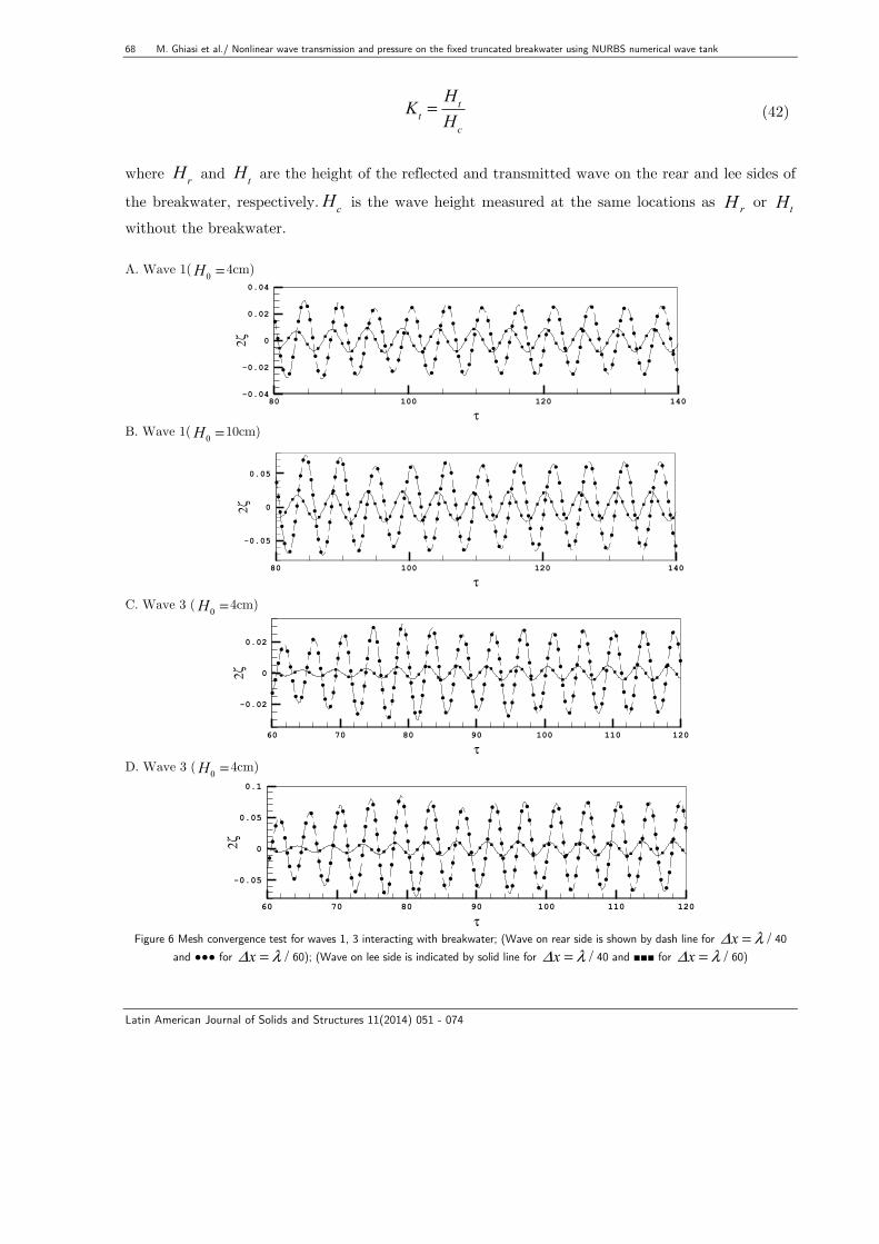
Two element sizes ( /xΔ λ= 40, /λ 60) are chosen to show time series wave evolution about body for the fourth order NURBS curve and interval time ( /t TΔ = 40) in Figure 6. It shows that the both solutions converge on both side of breakwater. CPU time is about 30% greater for the small mesh size.

Table 2 Incident wave characteristics.

No. ω rad s( ) d λ0 d λ Hmax λ H H0

Wave Steepness H λ

H0 = 4cm H0 = 10cm

1 5.23568 0.222392 0.2441 0.1294 0.9237 0.0180 0.0450 2 5.71198 0.264664 0.2807 0.1339 0.9375 0.0210 0.0526 3 6.28318 0.320244 0.3304 0.1376 0.9554 0.0252 0.0630 4 6.98131 0.395363 0.4006 0.1402 0.9751 0.0312 0.0780 5 7.85398 0.500381 0.5022 0.1415 0.9905 0.0396 0.0994 6 8.97597 0.653559 0.6538 0.1419 0.9988 0.0522 0.1304

Also, two time steps (Δt = T / 40, T / 80) are used to test solution convergence for mesh size

Δx = λ / 40 on the free surface and fourth order NURBS curve. Figure 7 shows the reflection and transmission of waves and solution time step convergence. CPU time of small time step is about 82% greater than the larger time step. Smoothing scheme is applied at every 20 time steps for high-er wave height of the waves 3 and 4.For other wave heights no smoothing scheme was required. Comparison of wave heights of transmitted wave and reflected wave shows that the reflection is magnified and transmission is shrunk when the incoming wave number becomes greater.

The wave energy dissipation of breakwater can be demonstrated by measuring the amount of wave energy reflected back to the rear side and transmitted past the breakwater. Wave reflection and transmission is quantified by the use of the wave reflection Kr and transmission Kt coeffi-cients written as:

Kr =Hr

Hc

(41)

x

y/d

5 10 15-1

-0.8

-0.6

-0.4

-0.2

0

0.2

Breakwater



Kt =Ht

Hc

(42)

where Hr and Ht are the height of the reflected and transmitted wave on the rear and lee sides of

the breakwater, respectively.Hc is the wave height measured at the same locations as rH or tHwithout the breakwater. A. Wave 1( 0H =4cm)

B. Wave 1( 0H =10cm)

C. Wave 3 ( 0H =4cm)

D. Wave 3 ( 0H = 4cm)

Figure 6 Mesh convergence test for waves 1, 3 interacting with breakwater; (Wave on rear side is shown by dash line for /xΔ λ= 40

and ●●● for /xΔ λ= 60); (Wave on lee side is indicated by solid line for /xΔ λ= 40 and ■■■ for /xΔ λ= 60)

τ

2ζ

80 100 120 140-0.04

-0.02

0

0.02

0.04

Lee side, dx = Landa/40Rear side, dx = Landa/40Lee side, dx = Landa/60Rear side, dx = Landa/60

τ

2ζ

80 100 120 140

-0.05

0

0.05

τ

2ζ

60 70 80 90 100 110 120

-0.02

0

0.02

τ

2ζ

60 70 80 90 100 110 120

-0.05

0

0.05

0.1



Reflection coefficient and transmission coefficient are depicted in Figure 8 for all waves. The higher the reflection coefficient, the lower transmission coefficient would be. It means that more portion of the wave energy is reflected and less portion of the wave energy is transmitted. Also, the reflection coefficient of the breakwater increases with the wave number. A. Wave 2( 0H =4cm)

B. Wave 2( 0H =10cm)

C. Wave 4 ( 0H =4cm)

D. Wave 4 ( 0H =4cm)

Figure 7 Time interval test for waves 2, 4 interacting with breakwater; (Wave on rear side is shown by dash line for /t TΔ = 40 and

●●● for /t TΔ = 80); (Wave on lee side is indicated by solid line for /t TΔ = 40 and ■■■ for /t TΔ = 80).

Wave force on the breakwater is computed by Equation 39. The first order backward finite dif-

ference method is used to evaluate time derivative of velocity potential over the breakwater surface and instantaneous hydrodynamics pressure. Time history of the horizontal and vertical forces on the

x (m)

2ζ 6 8 10 12 14

-0.02

0

0.02Breakwater

x (m)

2ζ 6 8 10 12 14

-0.05

0

0.05Breakwater

x (m)

2ζ 4 6 8 10 12

-0.02

0

0.02 Breakwater

x (m)

2ζ

4 6 8 10 12

-0.05

0

0.05

0.1Breakwater



breakwater ( Fx , Fz ) due to incident waves 1-6 are shown in Figure 9. The horizontal force is nor-

malized as 2Fx ρgBH and the vertical force is computed relative to the hydrostatic force and is

normalized as 2 Fz − ρgdB( ) ρgBH hence. It shows that horizontal forces are magnified when the

wave number becomes smaller.

Figure 8 The reflection and transmission coefficients of the fixed box-type breakwater.

Intersection points of free surface and the breakwater body moves and the number of elements

on the breakwater body changes at every time step. Hence, nonphysical instability occurs when finite difference formulation is used to obtain time derivation of velocity potential on instant wetted surface. It is called spike instability. Order of finite difference can influence time derivatives of ve-locity potential. Time series of the horizontal forces for waves 1 and 2 are shown in Figure 10, whereas ∂φ ∂t is obtained by first and second order backward finite difference. It shows that in the second order finite difference method instability occurs for some time steps while it does not occur at first order solution. Hence, for wave interaction with fixed bodies, first order finite differ-ence can be applied appropriately to compute ∂φ ∂t . 4 CONCLUSIONS

Numerical simulation of nonlinear wave interaction with a fixed structure at the two dimensional NURBS NWT is conducted in this paper. MEL method combined with high order boundary ele-ment method is applied to model the free surface distortion. High order boundary integral equation based on Green’s second identity and NURBS curve is employed to solve Laplace equation in the Eulerian frame. To obtain free surface elevation and re-gridding, NURBS interpolation is used. To update fully nonlinear free surface boundary condition in the Lagrangian manner, material node approach and fourth order Rung-Kutta time integration scheme are employed. Double node tech-nique is applied to overcome the difficulties arising from the singularity at the corner points.

w.w.B/g

Kr,Kt

0.5 1 1.5 2 2.50

0.5

1

1.5

2

KrKt

tHrH



A. Wave 1

B. Wave 2

C. Wave 3

D. Wave 4

E. Wave 5

F. Wave 6

Figure 9 Horizontal and vertical forces (ℑ= 2F ρgBH )on the breakwater for all waves;

(Dash line for horizontal force and solid line for vertical force)

τℑ

0 20 40 60 80 100 120

-0.5

0

0.5

τ

ℑ

0 20 40 60 80 100 120

-0.5

0

0.5

τ

ℑ

0 20 40 60 80 100 120

-0.5

0

0.5

τ

ℑ

0 20 40 60 80 100

-0.5

0

0.5

τ

ℑ

0 20 40 60 80

-0.4

-0.2

0

0.2

0.4

τ

ℑ

0 20 40 60 80-0.4

-0.2

0

0.2

0.4



The five points Chebyshev smoothing scheme is adopted to avoid instability of numerical procedure and to keep the accuracy of the solution within time marching scheme. Artificial damping zones (sponger layer) are placed at the both ends of the wave tank to absorb the wave energy to minimize reflection of the wave into the computational domain. An artificial wave maker is deployed by per-turbation sources over the length of inflow boundary. Normal flux of potential of a theoretical wave is feed into inflow boundary. A ramp function is applied to reduce the transient effect on the stabil-ity of solution.

A. Wave 1 B.Wave 2

Figure 10 Time history of horizontal force on the breakwater for incident wave 1 and 2

Different free surface mesh sizes and various order of NURBS curve are used to test convergence of NURBS NWT. CPU time and solution error are demonstrated for propagation nonlinear wave. The efficiency and performance of damping zone at the ends of NWT are addressed. A series of wav with different steepness is used to check the present numerical procedure for wave body interaction problem. Transmitted and reflected waves are studied for different wave numbers.

Wave vertical and horizontal forces on the breakwater are evaluated by first order and second order finite difference formulations. Instability of time derivative of velocity potential is addressed for both formulations. The results indicate that the present numerical method is an efficient tool for modeling the wave and fixed breakwater interactionin a numerical wave tank.

τ

ℑ

30 35 40 45 50-0.4

-0.2

0

0.2

0.4First order backwardSecond order backward

τ

ℑ

30 35 40 45 50-0.4

-0.2

0

0.2

0.4First order backwardSecond order backward



References

Bandyk, P.J., Beck, R.F. (2011). The acceleration potential in fluid-body interaction problems. Journal of Engi-neering Mathematics 70: 147-163. Büchmann, B., Skourup, J. and Cheung, K.F. (1998). Run-up on a structure due to second-Order waves and a current in a numerical wave tank. Journal of Applied Ocean Research 20: 297-308. Baudic, S.F., Williams, A.N., Kareem, A. (2001). A two-dimensional numerical wave flume-Part1; nonlinear wave generation, propagation, and absorption. OMAE Division and Presented at the 19th International Symposium and Exhibition on Offshore Mechanics and Arctic Engineering, New Orleans, USA. Boutros, Y.Z., Anwar, M. N. and Tewfick, A.H. (1986). Application of boundary integral equation method for modelling unsteady nonlinear water waves.Journal of Appling Mathematical Modeling 10: 11-15. Brebbia, C.A., Dominguez, I. (1992). Boundary elements: An introductory course, WIT Press. CAO, Y., Schultz, W.W. and Beck, R.F. (1991). Three-dimensional desingularized boundary integral method for potential problems. International Journal of Numerical Methods in Fluids.12: 758-803. Carbal, J.J.S.P, Worbel, L.C. and Brebbia C.A. (1990). A BEM formulation using B-splines: I- uniform blending functions. Engineering Analysis with Boundary Elements 7: 136-144. Carbal, J.J.S.P, Worbel, L.C. and Brebbia C.A. (1991). A BEM formulation using B-splines: I- multiple knots and non-uniform blending functions. Engineering Analysis with Boundary Elements 8: 51-55. Cointe, R. (1991). Free surface flows close to a surface piercing body. Mathematical Approaches in Hydrodynan-mics. Editors: T. Miloh. Soc. Ind. Appl. Math., Philadelphia. 319-334. Dean, R.G., Dalrymple, R.A., (1991). Water wave mechanics for engineers and scientists, World Scientific. Dommerth, D.(1987). Numerical methods for solving nonlinear water wave problems in the time domain, PhD Thesis, MIT .USA. Grilli, S.T., Svendsen, I.A.(1990). Corner problems and global accuracy in the boundary element solution of non-linear wave flow. Journal of Engineering Analysis with Boundary Elements 7: 178-195. Hamano, K., Murashige, S. and Hayami. K.(2003). Boundary elements simulation of large amplitude standing waves in vessels. Journal of Engineering Analysis with BoundaryElopements 27: 565-574. Hsin, C.Y., Kerwin, J.E. and Newman, J.N.(1993). A high-order panel method for ship motions based on B-Splines. In Proceeding 6th International Conference on Numerical Ship Hydrodynamics, Iowa. Kim, B., Shin Y.S.(2003). A NURBS panel method for three-dimensional radiation and diffraction problems. Journal of Ship Research.47: 177-186. Koo, W.(2003). Fully nonlinear wave-body interaction by a 2D potential numerical wave tank, PhD Thesis, Tex-as A&M University. USA. Koo, W., Kim, M.H.(2004).Nonlinear wave-floating body interactions by a 2D fully nonlinear numerical wave tank.Proceeding 14th International Offshore and Polar Engineering Conference, Toulon, France, 23-28. Li, Y.S., Liu, S.X., Yu. Y.X. and Lai. G.Z.(2000).Numerical modelling of multi-directional irregular waves through breakwaters.Journal of Applied MathematicalModeling 24: 551-574. Longuet-Higgins, M.S., Cokelet, E.D.(1976). The deformation of steep surface waves on water (Ι)-a numerical method of computation. Proceeding of The Royal Society of London, Series A, 350, 1-26. Newman, J.N.(1989). Marine hydrodynamics. 6th ed., MIT Press. Newman, J.N. (2010). Analysis of wave generators and absorbers in basins.Journal ofApplied Ocean Research.32: 71-82. Ning, D.Z., Teng, B.(2006).Numerical simulation of fully nonlinear irregular wave tank in three dimension nu-merical wave tank. International Journal Numerical Methods in Fluids.53: 1847-1862. Park, J.C., Kim, M.H., Miata, H. and Chun, H.H.(2003). Fully nonlinear numerical wave tank (NWT) simula-tion and wave Run-Up prediction around 3D Structure. Ocean Engineering 20: 1969-1996. Park, J.C., Kim, M.H. andMiyata, H.(1999). Fully non-linear free-surface simulation by a 3D viscous numerical wave tank.International Journal of Numerical Methods in Fluids.29: 685-703.



Park, J.C., Kim, M.H. and Miyata, H.(2001). Reproduction of fully-nonlinear multi-directional waves by a 3D viscous numerical wave tank. In proceeding of The 11th International Offshore and Polar Engineering Conference, Stavanger, Norway. Ryu, S., Kim, M.H. and Lynett P.J.(2003).Fully nonlinear wave-Current interactions and kinematics by a BEM-based numerical wave tank.Journal of Computational. Mechanics. 32: 336-346. Tanizawa, K.(2000). The state of the art on numerical wave tank.In Proceeding of 4th Osaka Colloquium on Sea-keeping Performance of Ships, Japan, 95-114. Tang, H.J. & Huang, C.C, (2008).Bragg reflection in a fully nonlinear numerical wave tank based on boundary integral equation method. Ocean Engineering. 35: 1800-1810. Tiller, w.(1996).NURBS book, Springer. Wang, C.Z., Wu, G.X.(2010). Interaction between fully nonlinear water waves and cylinder arrays in a wave tank. Ocean Engineering. 37: 400-417. Wu, N.J., Tsay, T.K. and Young D.l.(2005).Meshless numerical simulation for fully nonlinear water waves.International Journal of Numerical Methods in Fluids.50: 219-234. Xiao, L.F., Yang, J.M., Peng, T. and Li, J.(2009). A meshless numerical wave tank for simulation of nonlinear ir-regular waves in shallow Water.International Journal of Numerical.Methods in Fluids.61: 165-184. Xü, H., Yue, D.K.P.(1992). Computation of fully-nonlinear three Dimensional water waves. Proceeding of 19th Symposium on Naval Hydrodynamics, Seoul, Korea. Zhang X.T., Khoo, B.C. and Lou, J.(2005). Wave propagation in a fully nonlinear numerical wave tank: A des-ingularized method. Ocean Engineering 33: 2310-2331.

nonlinear wave transmission and pressure on the fixed ... · 52 m. ghiasi et al./ nonlinear wave...

Documents