nonlinear statistical methodology applied on modeling the...

Nonlinear Statistical Methodology Applied on Modeling the Growth Correlation of Some Global Macroeconomic Parameters

1

Nonlinear Statistical Methodology Applied on Modeling the Growth Correlation of Some Global Macroeconomic ParametersAssoc. Prof. Dr. Ivan MihajlovicManagement Department, Technical Faculty in Bor, University in Belgrade, Serbiaemail: [email protected]

Assist. Prof. Aleksandra Fedajev, MScManagement Department, Technical Faculty in Bor, University in Belgrade, Serbiaemail: [email protected]

Assist. Prof. Ivica Nikolic, MScManagement Department, Technical Faculty in Bor, University in Belgrade, Serbiaemail: [email protected]

Prof. Dr. Zivan ZivkovicManagement Department, Technical Faculty in Bor, University in Belgrade, Serbiaemail: [email protected]

Primena nelinearnih statističkih metoda na modeliranje korelacije rasta kod nekih globalnih makroekonomski parametraDr. Ivan Mihajlović, Vanredni ProfesorKatedra za menadžment, Tehnički fakultet u Boru, Univerzitet u Beogradu, Srbijaemail: [email protected]

Aleksandra Fedajev, AsistentKatedra za menadžment, Tehnički fakultet u Boru, Univerzitet u Beogradu, Srbijaemail: [email protected]

Ivica Nikolić, Asistent Katedra za menadžment, Tehnički fakultet u Boru, Univerzitet u Beogradu, Srbijaemail: [email protected]

Dr. Živan Živković, Redovni professorKatedra za menadžment, Tehnički fakultet u Boru, Univerzitet u Beogradu, Srbijaemail: [email protected]

Abstract: This paper presents the preliminary results of modeling the interdependence between some macroeconomic parameters which included daily goods prices: Gold price, Brent Oil price, Copper price, Natural gas price; exchange rates: USD to JPY, EUR to USD, EUR to JPY and the stock market indices: S&P 500 index, Dow Jones Industrial index, EURO Stoxx 50 index, Nikkei 225 index, Dow Jones Composite index and the Dow Jones Global index. Listed parameters were being continually recorded for the period of nine months. Subsequently, data collected were statistically processed in order to determine the param-eter with the driving effect. This was followed by an attempt to develop further the conceiv-able model of their interdependence.

Ivan Mihajlovic, Aleksandra Fedajev, Ivica Nikolic and Zivan Zivkovic

2

І. Introduction

The issue of this analysis is an attempt to develop the model of interdependency between some globally important mac-roeconomic parameters, especially in the context of global economy development. There were attempts to do similar mod-eling in contemporary scientific literature, coming from different fields of sciences. However, most of authors attempted to develop connection among stock markets and initial conditions of the external mar-ketplaces. The aim of such analysis was to develop model that could predict the dynamics of stock markets change. The stock markets are said to be nonlinear, dy-namic systems. Chaos theory is the math-ematics of studying such nonlinear, dy-namic systems (Banks et al., 2003). Does this mean that scientists dealing with the chaos theory can predict when stocks will rise and fall? Not quite; however, during research and modeling in previous dec-ades, it was determined that the market prices are highly random, but with a trend. The stock market is accepted as a self-similar system in the sense that the indi-vidual parts are related to the whole. Also, it was discovered, that the stock market has sensitive dependence on initial condi-tions. This factor is what makes dynamic market systems so difficult to predict. Be-cause it is hard to describe accurately the current situation with the necessary detail, it is most difficult to predict accurately the state of the system at a future time (Finn-track Ltd, 2011). In this way, short-term investing, such as intraday exchanges, is an item which cannot be predicted accu-rately enough. However, over time, long-

І. Uvod

Tema ove analize je pokušaj da se razvije model međuzavisnosti između nekih glo-balno značajnih makroekonomskih para-metara, posebno u kontekstu globalnog ekonomskog razvoja. U savremenoj nauč-noj literaturi bilo je pokušaja da se ura-de slična modelovanja, koja su dolazila iz različitih naučnih oblasti. Međutim, većina autora je pokušala da razvije vezu između berza i početnih uslova spoljnog tržišta. Cilj takve analize bio je da se razvije model koji bi mogao da predvidi dinamiku ber-zanskih promena. Za berze se smatra da su to nelinearni, dinamički sistemi (Banks i dr., 2003). Da li to znači da naučnik koji se bavi teorijom haosa može predvideti kada će akcije rasti ili opasti? Pa ne baš; me-đutim, tokom istraživanja i modelovanja u prethodnim decenijama, utvrđeno je da se tržišne cene ponašaju stohastički ali sa trendom. Berza je prihvaćena kao pose-ban sistem u kome su pojedinačni delovi u vezi sa celinom. Takođe, otkriveno je da berza ima osetljivu zavisnost od početnih uslova. Ova činjenica je ono što čini dina-mički sistem tako teškim za predviđanje. Zbog toga što je teško precizno opisati trenutnu situaciju sa svim neophodnim detaljima, najteže je precizno predvideti stanje sistema u budućem periodu (Finn-track Ltd, 2011). Na ovaj način kratkoroč-na ulaganja, kao što su dnevne razmene, predstavljaju stavke koje ne mogu biti predviđene dovoljno precizno. Međutim, tokom vremena, dugoročna cena akcija nije slučajna. Trgovci mogu uspešno trgo-vati sa dnevnim ili nedeljnim vrednostima ako prate trendove. Prema tome, sistem

Key words: quantitative methods, macroeconomic effects, modeling, nonlinear statistics.

Izvod: U ovom radu su prikazani preliminarni rezultati modeliranja međuzavisnost po-jedinih makroekonomskih parametara u koji ulaze cene sledećih roba: cena zlata, cena Brent nafte, cena bakra, cena prirodnog gasa; deviznih kurseva: USD prema JPY, EUR prema USD, EUR prema JPY i Berzanskih indeksa: S&P 500 indeks, Dow Jones Industri-als indeks, EURO Stoxx 50 indeks, Nikkei 225 indeks, Dow Jones Composite indeks i Dow Jones Global indeks. Navedeni parametri su kontinuirano praćeni za period od devet mese-ci. Nakon toga, prikuplјeni podaci su statistički obrađeni u cilјu određivanja parametra koji ima upravljački efekat. Ovo je bilo praćeno sa pokušajem da se dodatno razvije primenljiv model njihove međuzavisnosti.

Ključne reči: kvantitativne metode, makroekonomski efekti, modelovanje, nelinearne statistike.

JEL Classification: C3, C8


3

term price action is not random. Traders can succeed trading from daily or weekly charts if they follow the trends. According-ly, a system can be random in the short-term and deterministic in the long term.

Considering that the stock markets could be connected to the chaos theory, most of the non-specialists have an opinion on the chaos theory as a complicated item which should be considered only by scientists and scholars. This opinion was disapproved in this next sentence, written at the end of the book A Brief History of Time (Hawking, 1998):” If we do discover a complete the-ory, it should in time be understandable in broad principle by everyone, not just a few scientists. Then we shall all, philoso-phers, scientists, and just non-specialists, be able to take part in the discussion of the question of why it is that we and the universe exist.” The meaning is that the chaos theory cannot be complete until it becomes understandable to the general public.

Accordingly, there were attempts in which the stock markets were modeled by avail-able mathematical tools. For example, there is an example which is based on data collected about Dow Jones Indus-trial stock prices, divisor, and average at month’s close from December 31, 1990, to October 31, 1998, then extrapolated and displayed (DJI) prices, divisor, and aver-age to 2001. This example was integrated as a tool in a MLAB (Civilized Software, Inc), as a demonstration file. However, one should have in mind that the base of this model was created from the data ob-tained in the period 1990 to 1998, so it is not realistic to expect higher accuracy of long term extrapolation, because of the phenomena which Edward Lorentz firstly realized in the early 1960’s (Lorenz, 1963; Lorenz, 1966; C.A.Danforth, 2001). The findings of Professor Lorenz relied on the theory of large number rows. In the case of large row of number modeling, the ac-curacy will increase if the extrapolation is not too far from the borders of considered data set. This is because of the fact that in the dynamic systems, equilibrium states are changing their position in time. Moving far in extrapolation, will probably neglect the formation of some new equilibrium state in the future, which is dependence

može biti slučajan u kratkom roku i deter-ministički u dugom roku.

S obzirom da berze mogu biti povezane te-orijom haosa, većina onih koji nisu struč-ni u datoj oblasti imaju mišljenje o teoriji haosa kao o jednoj komplikovanoj oblasti koja bi trebala biti razmatrana samo od strane naučnika. Ovaj stav je osuđivan u sledećoj rečenici, napisanoj na kraju knji-ge čiji je naziv Kratka istorija vremena (Hawking, 1998): „ Ako radimo na tome da otkrijemo komplektnu teoriju, ona bi trebala da na vreme bude razumljiva u ši-rokim načelima od strane svih, a ne samo od nekoliko naučnika. Tada će svi, filozo-vi, naučnici i čak nestručni pojedinci, biti sposobni da učestvuju u diskusijama na pitanje zašto mi i svemir postojimo.“ Smi-sao je u tome da teorija haosa ne može biti potpuna dok ne postane razumljiva od strane široke populacije.“

Prema tome, bilo je pokušaja u kojima su berze bile modelirane primenom raspolo-živih matematičkih alata. Na primer, tu je slučaj koji se zasniva na prikuplјenim po-dacima o Dow Jones Industrial ceni akcija, odnosu i proseku na mesečnom zatvaranju 31. decembra 1990, do 31. oktobra 1998, zatim je izvedena vrednost i predstavljene (DJI) cene, odnos i prosek za 2001. Ovaj primer je integrisan kao alat u MLAB (Ci-vilized Software, Inc), kao pokazna dato-teka. Međutim, treba imati na umu da je osnova ovog modela nastala na osnovu podataka dobijenih u periodu od 1990. go-dine do 1998. godine, tako da nije realno očekivati veću tačnost u dugoročnoj prime-ni, zbog fenomena koji je Edward Lorentz prvi predstavio u ranim 1960-tim (Lorenz, 1963; Lorenz, 1966; C.A.Danforth, 2001). Nalazi profesora Lorenz-a oslanjali su se na teoriji redova velikih brojeva. U slučaju modeliranja velikog broja redova, tačnost će se povećati ako ekstrapolacija nije su-više daleka od granice razmatranog sku-pa podataka. Ovo je zbog činjenice što u dinamiočkim sistemima, ravnotežna sta-nja menjaju svoje položaje u vremenu. Udaljavanje ekstrapolacijom, verovatno će zanemariti formiranje neke nove budu-će ravnoteže, što će zavisiti od promene spoljnih uslova sistema.

Naravno, posle tih prvih pokušaja, bilo je


4

on change of external conditions of the system.

Off course, after those first attempts, there was further development of such math-ematical modeling (Bullard and Batler, 1993; Takala and Viren, 1996; Murphy, 1996; Perrelo et al., 2994; Guegan, 2009). What could be concluded from referenc-es published in recent years is that new trends in modeling stock market data were based on acceptance of different equilib-rium states through which financial indi-cators pass during the period of record-ing and observations. Those equilibrium states could be defined as macroeconomic phases in time series of each considered indicator, such are Dow Jones, NASDAQ, SP500, NIKKE, etc. (Wong, et al., 2009). Thus, increasing the period of observation increases the number of potential equilib-rium states. Each equilibrium state is usu-ally placed in different amplitude of input and output parameters, requiring discrete model equation. This fact limits the appli-cability of modeling methods based on lin-ear statistical approach (such is MLRA) or even methods based on nonlinear statisti-cal approach with “one rule” input variable (such are ANNs).

Accordingly, modeling approaches de-scribed in recent references are mostly based on methodologies which take into consideration the change of scopes of in-put and output variables in time, depend-ing on the number of equilibrium states of the system. Some of the interesting ap-proaches are given in the manuscript re-cently published by Juarez (Juarez 2010). In this manuscript the author deals with defining the relations among the aggre-gate financial indicators based on the Lor-enz equation, which cluster the input data around different equilibrium states, pro-ducing adequate model equation for each one. Another approach published in recent years is based on a multivariate Markov Switching Intercept Autoregressive Het-eroscedasticity (MSIAH) models, which is also used for more than one rule (regime) of input variable observed during longer time series (Chan et al., 2011).

The analysis presented in this paper is based on a new approach of assessing the macroeconomic data collected, e.g. the stock prices, the exchange rates and the

daljih razvoja takvog matematičkog mo-delovanja (Bullard i Batler, 1993; Takala i Viren, 1996; Murphy, 1996; Perrelo i dr., 2004; Guegan, 2009). Ono što se može zaključiti iz referenci objavljenih u posled-njih nekoliko godina jeste da su novi tren-dovi u modeliranju berzanskih podataka zasnovani na prihvatanju drugačijih rav-notežnih stanja kroz čije finansijske indi-katore prolazimo tokom perioda snimanja i posmatranja. Ta ravnotežna stanja mogla bi se definisati kao makroekonomske faze u vremenskim serijama svakog posma-tranog indikatora kao što su Dow Jones, NASDAQ, SP500, NIKKE, itd. (Wong, i dr., 2009). Na ovaj način povećenjem perioda posmatranja povećava se broj potencijal-nih ravnotežnih stanja. Svako ravnotežno stanje je obično stavljeno u različitim am-plitudnim ulazima i izlaznim parametrima, zahtevajući diskretnu jednačinu modela. Ova činjenica ograničava primenjivost me-toda modeliranja koji se zasnivaju na pri-stupu linearne statistike (takva je MLRA) ili čak metode koje su zasnovani na neli-nearnom statističkom pristupu sa „jednim pravilom“ promene ulazne varijable (kao što su ANN).

Prema tome, pristupi modelovanja opi-sanih u poslednjih nekoliko referenci su uglavnom zasnovani na metodologijama koje uzimaju u obzir promene opsega ula-znih i izlaznih promenljivih tokom vreme-na, u zavisnosti od broja ravnotežnih sta-nja sistema. Neki od zanimljivih pristupa dati su u rukopisu nedavno objavljenih od strane Juarez-a (Juarez 2010). U ovom ru-kopisu autor se bavio definisanjem odnosa između ukupnih finansijskih pokazatelјa na osnovu Lorenz-ove jednačine, koji klasira ulazne podatke oko različitih rav-notežnih stanja, proizvodeći adekvatnu jednačinu modela za svaku od njih. Dru-gi pristup objavljen u poslednjih nekoliko godina je zasnovan na multivarijabilnim “Markov Switching Intercept Autoregressi-ve Heteroscedasticity“ (MSIAH) modelima, koji su takođe korišćeni za više od jednog pravila (režima) ulaznih varijabli posma-trane tokom duže vremenske serije (Chan i dr., 2011).

Analiza predstavlјena u ovom radu za-snovana je na novom pristupu procene prikuplјenih makroekonomskih podataka


5

npr. cene akcija, devizni kursevi i cene robe, sa cilјem da se pronađe njihova međusobna korelacija i mogućnost da se predvide promene u njihovim trendovima.

II. Podaci

Podaci u uzorku, korišćeni za proračune u ovom radu sastoje se od dnevne varijaci-je cene roba: cene zlata (X1), cene Brent nafte (X2), cene bakra (X3), cene prirod-nog gasa (X4); valutnih kurseva: USD prema JPY (X5), EUR prema USD (X6), EUR prema JPY (X7) i berzanskih indeksa: S&P 500 indeks (X8), Dow Jones Industrial indeks (X9), EURO Stoxx 50 indeks (X10), Nikkei 225 indeks (X11), Dow Jones Com-posite indeks (X12) i Dow Jones Global in-deks (Y).

Većina tih vrednosti su dobijene sa sajta ForexPros (finansijsko tržište širom sveta) i Dow Jones zvaničnog veb sajta. Najvaž-niji parameter, koji je bio predmet izuča-vanja, za finalni model bio je globalni DJI (Y).

Vrednosti navedenih parametra su priku-pljeni na dnevnom nivou i to na zatvara-nju berza, počev od 2. januara 2012. go-dine a završavajući 28. septembra 2012. godine. Dakle, početna baza podataka, sa 195 vektora iz 13 dimenzija bila je formi-rana na ovaj način. Treba napomenuti da cene metala (zlata i bakra) nisu raspolo-žive tokom vikenda, iz tog razloga, za sve 13 varijable nisu uzeti u obzir podaci koji postoje vikendom. Zatim, dobijeni podaci su standardizovani u odnosu na početnu vrednost (dobijenu u prvom danu mere-nja), kako bi se dobila stopa promene u određenom vremenskom periodu. Na ovaj način sve praćene varijable zapravo pred-stavljaju stope promena, koje su od po-sebnog značaja za dalji pristup diskutovan u ovom radu.

III. Eksperimentalna metodologija

Eksperimentalni pristup iz koga su dobije-ni rezultati prikazani u ovom radu zasni-va se na novom pristupu, definisanog kao „efekat-bove“. Za sve posmatrane varija-ble (X1 do X2 i Y), rang (R) je bio izra-čunat počevši od prvog dana posmatranja (2. januara 2012). Zatim, su sve varijable bile rangirane prema vrednosti ranga (R)

goods prices, with the aim to find their in-ter correlations and the possibility to pre-dict the change in their trends.

II. The Data

The sample data, used for calculations in this paper, consist of daily goods prices: Gold price (X1), Brent Oil price (X2), Cop-per price (X3), Natural gas price (X4); exchange rates: USD to JPY (X5), EUR to USD (X6), EUR to JPY (X7) and the stock market indices: S&P 500 index (X8), Dow Jones Industrial index (X9), EURO Stoxx 50 index (X10), Nikkei 225 index (X11), Dow Jones Composite index (X12) and the Dow Jones Global index (Y).

Most of those values were obtained from ForexPros (Financial markets worldwide) and Dow Jones official web site. The most important parameter, which was the sub-ject of intent, for our final model was the global DJI (Y).

The values of the above mentioned pa-rameters have been collected on a daily base, at market closure, starting from January 2nd 2012 and ending with Sep-tember 28th 2012. Thus, a starting data base with 195 vectors of 13 dimensions was formed. It should be noted that the metal prices (gold and copper) are not available during weekends, so the week-end data was not taken into considera-tion for all 13 variables. Then, the results obtained have been standardized in com-parison to the starting value (obtained on the first day of measurement), to obtain the rate of change during the period. This way all investigated variables actually are the rates of change, which are of particu-lar interest for further modeling approach discussed in the paper.

III. Experimental methodology

The experimental approach behind the re-sults presented in this paper is based on a new approach. We defined it as a “buoy-effect”. For all indicated variables (X1 to X12, and Y), the range (R) has been calcu-lated starting from the first day of obser-vation (January the 2nd 2012). Then, all variables have been ranked according to the values of their ranges (R) during time series. The variable with higher range is


6

selected as the central “buoy”. If the level of correlation of this variable with the rest of the explanatory variables is high; then, its relative change causes the change of all connected variables, instantaneously. In such cases, interdependence of cor-related variables could be modeled using linear approach (MLRA). If the degree of correlation between two variables is not high, this doesn’t automatically mean that the behavior of one variable does not in-fluence the behavior of another. This just indicates that their inter correlation can-not be described with the linear model, but modeling based on dynamic behavior of the variables can be used to present the behavior of the variables in the future. Then, modeling could be facilitated by the usage of nonlinear statistical approach such as Artificial Neural Networks (ANNs), in the case that all variables do not have a wide range of change during the whole time interval of observation, or Adaptive-Network-Based Fuzzy Inference System for variables with wide range of change.

IV. Results and discussions

After standardization of the 13 factors considered, descriptive statistics has been calculated for all the data and the results are presented in Table 1.

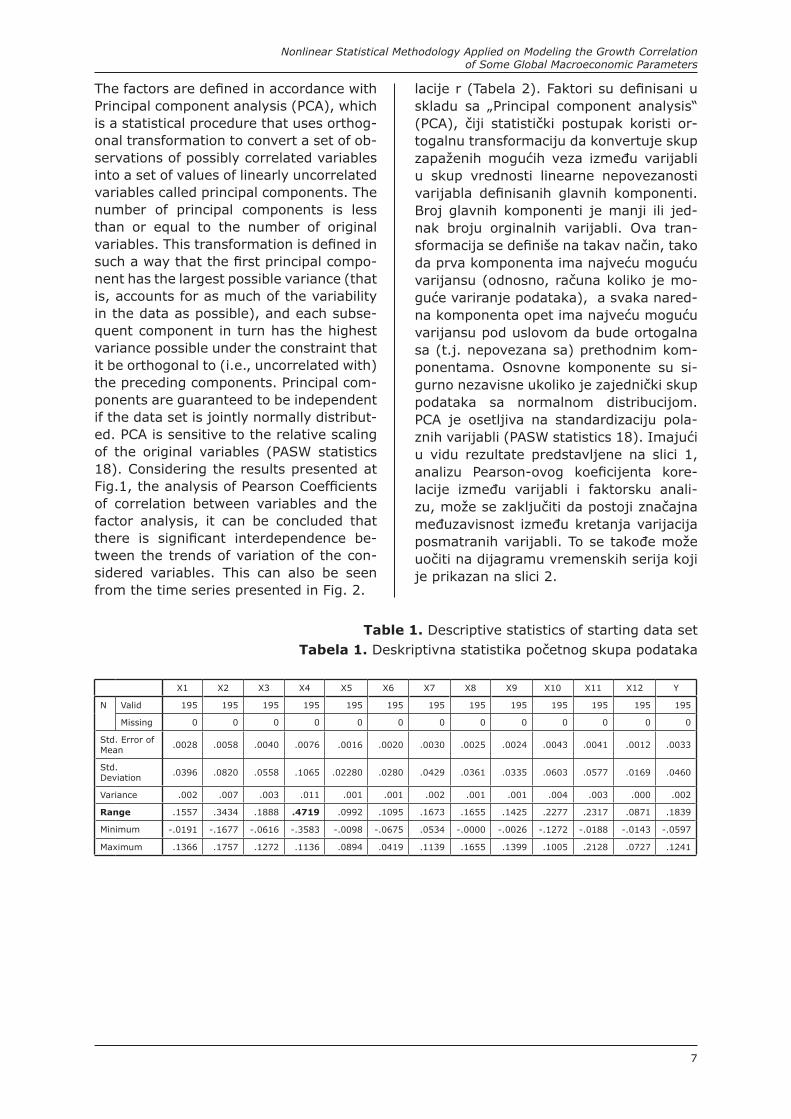
According to the values of the Range (Ta-ble 1), the central “buoy” has been identi-fied. The variable with the largest range is the variable X4 (the natural gas price). The residual variables have been subse-quently lined according to ranges, on the left and right side of the central buoy (X4), as presented in Fig. 1.

Future analysis included the Pearson Co-efficients (PC) calculation between the output (Y) and all input variables. Almost all PC values obtained were positive and with values above 0.5, having statistical significance (p < 0.01). The only excep-tion was the correlation between Y and X4 (r = -0.302; p < 0.01), which is starting the trend of other variables changes, ac-coriding to Fig.1. Also, factor analysis in-dicated that all variables can be divided in two factor groups. First factor contains most of the variables, and the second one contains only variables X4 and X5, how-ever in inverse inter correlation (Table 2).

u toku vremenske serije. Promenljiva sa najvišim rangom je odabrana kao central-na „bova“. Ako je stepen korelacije ove varijable sa ostalim varijablama visok; tada njena relativna promena prouzrokuje trenutne promene svih ostalih povezanih promenljivih. U takvim slučajevima, me-đuzavisnost povezanih varijabli može se modelovati korišćenjem linearnog pristu-pa (MLRA). Ako stepen korelacije između dve promenljive nije visok, to automatski ne znači da ponašanje jedne varijable ne utiče na onašanje drugih. To nam samo ukazuje da njihova međupovezanost ne može biti opisana linearnim modelom, ali modelovanje zasnovano na dinamičkom ponašanju varijabli može biti korišćeno za predstavljanje ponašanja promenljivih u budućnoti. Tako da modeliranje može biti olakšano korišćenjem nelinearnih statistič-kih pristupa kao što su Veštačke neuron-ske mreže (ANN), u slučaju u kom sve va-rijable nemaju širok rang promene u toku celog vremenskog intervala posmatranja, ili ANFIS metodu za varijable sa širokim rangom promene.

IV. Rezultati i diskusija

Nakon standardizacije 13 razmatranih pa-rametra, izračunata je deskriptivna stati-stiaka za sve podatke čiji su rezultati pri-kazani u Tabeli 1.

Prema vrednostima ranga (Tabela 1), određena je centralna „bova“. Promenljiva sa najvećim opsegom je X4 (cena prirod-nog gasa). Preostale promeljive su zatim postavljene prema rangu na levoj i desnoj strani od centralne bove (X4), kao što je prikazano na Slici 1.

Buduća analiza obuhvata „Pearson Coeffi-cients“ (PC) izračunat između izlaza (Y) i svih ulaznih promenljivih. Skoro sve po-smatrane PC vrednosti bile su pozitivne sa vrednostima preko 0.5, imajući statističku značajnost (p < 0.01). Jedini izuzetak bila je korelacija između Y i X4 (r = -0.302; p < 0.01), koja započinnje trend prome-ne ostalih varijabli, kao na slici 1. Tako-đe, faktorska analiza je pokazala da sve varijable možemo podeliti u dve faktorske grupe. Prva faktor sadrži najviše varija-bli, a drugi sadrži samo variable X4 i X5, međutim sa obrnutim koeficijontom kore-


7

The factors are defined in accordance with Principal component analysis (PCA), which is a statistical procedure that uses orthog-onal transformation to convert a set of ob-servations of possibly correlated variables into a set of values of linearly uncorrelated variables called principal components. The number of principal components is less than or equal to the number of original variables. This transformation is defined in such a way that the first principal compo-nent has the largest possible variance (that is, accounts for as much of the variability in the data as possible), and each subse-quent component in turn has the highest variance possible under the constraint that it be orthogonal to (i.e., uncorrelated with) the preceding components. Principal com-ponents are guaranteed to be independent if the data set is jointly normally distribut-ed. PCA is sensitive to the relative scaling of the original variables (PASW statistics 18). Considering the results presented at Fig.1, the analysis of Pearson Coefficients of correlation between variables and the factor analysis, it can be concluded that there is significant interdependence be-tween the trends of variation of the con-sidered variables. This can also be seen from the time series presented in Fig. 2.

lacije r (Tabela 2). Faktori su definisani u skladu sa „Principal component analysis“ (PCA), čiji statistički postupak koristi or-togalnu transformaciju da konvertuje skup zapaženih mogućih veza između varijabli u skup vrednosti linearne nepovezanosti varijabla definisanih glavnih komponenti. Broj glavnih komponenti je manji ili jed-nak broju orginalnih varijabli. Ova tran-sformacija se definiše na takav način, tako da prva komponenta ima najveću moguću varijansu (odnosno, računa koliko je mo-guće variranje podataka), a svaka nared-na komponenta opet ima najveću moguću varijansu pod uslovom da bude ortogalna sa (t.j. nepovezana sa) prethodnim kom-ponentama. Osnovne komponente su si-gurno nezavisne ukoliko je zajednički skup podataka sa normalnom distribucijom. PCA je osetljiva na standardizaciju pola-znih varijabli (PASW statistics 18). Imajući u vidu rezultate predstavljene na slici 1, analizu Pearson-ovog koeficijenta kore-lacije između varijabli i faktorsku anali-zu, može se zaključiti da postoji značajna međuzavisnost između kretanja varijacija posmatranih varijabli. To se takođe može uočiti na dijagramu vremenskih serija koji je prikazan na slici 2.

Table 1. Descriptive statistics of starting data setTabela 1. Deskriptivna statistika početnog skupa podataka

X1 X2 X3 X4 X5 X6 X7 X8 X9 X10 X11 X12 Y

N Valid 195 195 195 195 195 195 195 195 195 195 195 195 195

Missing 0 0 0 0 0 0 0 0 0 0 0 0 0

Std. Error of Mean .0028 .0058 .0040 .0076 .0016 .0020 .0030 .0025 .0024 .0043 .0041 .0012 .0033

Std. Deviation .0396 .0820 .0558 .1065 .02280 .0280 .0429 .0361 .0335 .0603 .0577 .0169 .0460

Variance .002 .007 .003 .011 .001 .001 .002 .001 .001 .004 .003 .000 .002

Range .1557 .3434 .1888 .4719 .0992 .1095 .1673 .1655 .1425 .2277 .2317 .0871 .1839

Minimum -.0191 -.1677 -.0616 -.3583 -.0098 -.0675 .0534 -.0000 -.0026 -.1272 -.0188 -.0143 -.0597

Maximum .1366 .1757 .1272 .1136 .0894 .0419 .1139 .1655 .1399 .1005 .2128 .0727 .1241


8

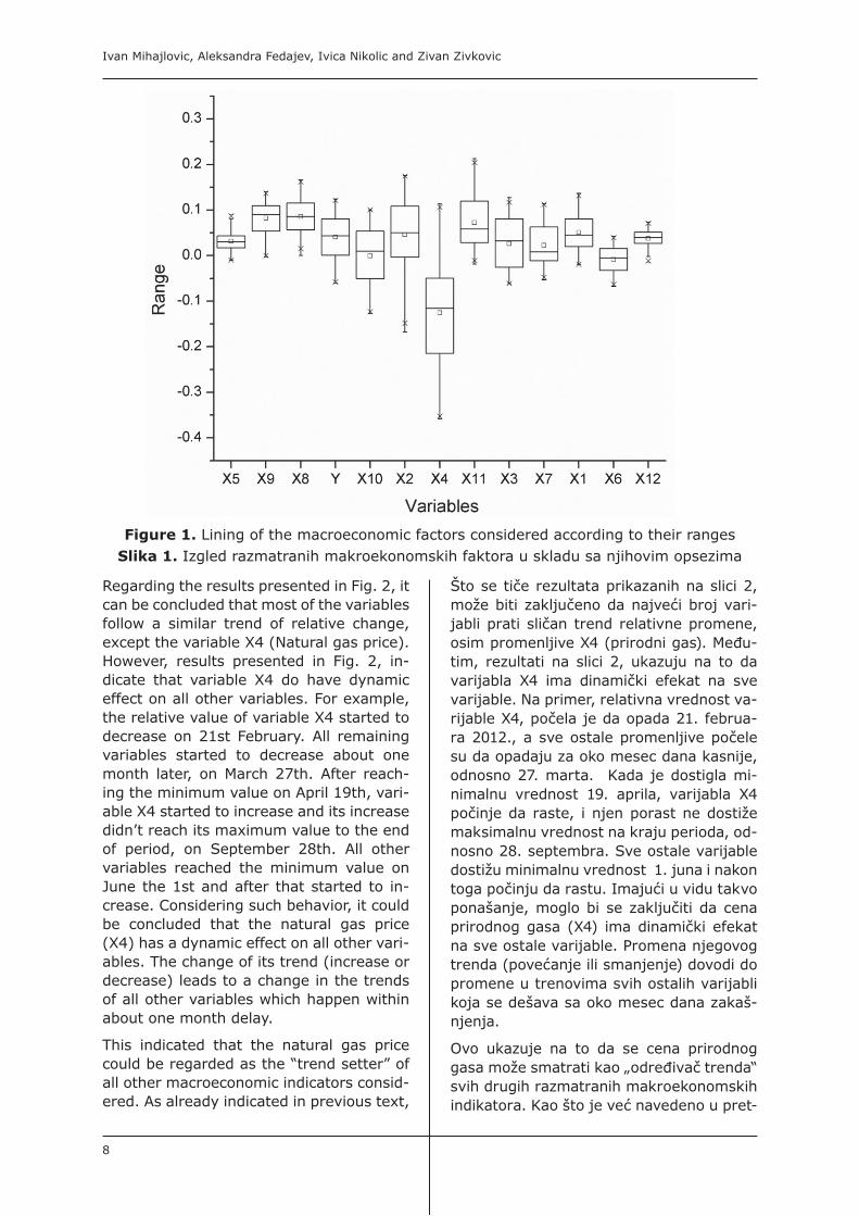
Regarding the results presented in Fig. 2, it can be concluded that most of the variables follow a similar trend of relative change, except the variable X4 (Natural gas price). However, results presented in Fig. 2, in-dicate that variable X4 do have dynamic effect on all other variables. For example, the relative value of variable X4 started to decrease on 21st February. All remaining variables started to decrease about one month later, on March 27th. After reach-ing the minimum value on April 19th, vari-able X4 started to increase and its increase didn’t reach its maximum value to the end of period, on September 28th. All other variables reached the minimum value on June the 1st and after that started to in-crease. Considering such behavior, it could be concluded that the natural gas price (X4) has a dynamic effect on all other vari-ables. The change of its trend (increase or decrease) leads to a change in the trends of all other variables which happen within about one month delay.

This indicated that the natural gas price could be regarded as the “trend setter” of all other macroeconomic indicators consid-ered. As already indicated in previous text,

Što se tiče rezultata prikazanih na slici 2, može biti zaključeno da najveći broj vari-jabli prati sličan trend relativne promene, osim promenljive X4 (prirodni gas). Među-tim, rezultati na slici 2, ukazuju na to da varijabla X4 ima dinamički efekat na sve varijable. Na primer, relativna vrednost va-rijable X4, počela je da opada 21. februa-ra 2012., a sve ostale promenljive počele su da opadaju za oko mesec dana kasnije, odnosno 27. marta. Kada je dostigla mi-nimalnu vrednost 19. aprila, varijabla X4 počinje da raste, i njen porast ne dostiže maksimalnu vrednost na kraju perioda, od-nosno 28. septembra. Sve ostale varijable dostižu minimalnu vrednost 1. juna i nakon toga počinju da rastu. Imajući u vidu takvo ponašanje, moglo bi se zaključiti da cena prirodnog gasa (X4) ima dinamički efekat na sve ostale varijable. Promena njegovog trenda (povećanje ili smanjenje) dovodi do promene u trenovima svih ostalih varijabli koja se dešava sa oko mesec dana zakaš-njenja.

Ovo ukazuje na to da se cena prirodnog gasa može smatrati kao „određivač trenda“ svih drugih razmatranih makroekonomskih indikatora. Kao što je već navedeno u pret-

Figure 1. Lining of the macroeconomic factors considered according to their rangesSlika 1. Izgled razmatranih makroekonomskih faktora u skladu sa njihovim opsezima


9

factor analysis of the variables presented in table 2, revealed another interesting re-sult. Namely, all variables are extracted in two factors, with the second factor includ-ing natural gas price (X4) and USD/JPY exchange rate. Those two variables are contained in the same factor with opposite factor loadings. This means that increase of natural gas price will automatically lead to decrease of USD/JPY ratio. So, it can be concluded that increase of natural gas price will lead to strengthening of JPY or decline of USD. This trend is not unexpected, con-sidering that Japan is a larger importer of natural gas. This correlation becomes es-pecially important after the Japan’s nuclear crisis. The expansion of Japanese industry after the nuclear crisis led to almost con-stant decrease of USD/JPY ratio. This, of course, caused the increase of the Japa-nese industry’ natural gas demand (Er-man, 2011), because of the substitution of the nuclear power and oil consumption with usage of natural gas (Nakajima and Hamori, 2012). Increased natural gas de-mand leads to rise of its price. Having this in mind, it could be concluded that there is a significant direct – negative - correlation between the natural gas price and USD/JPY ratio (Component 2 in Table 2). On the other hand, natural gas price is dynami-cally correlated with all other considered macroeconomic parameters included in Component 1 of Table 2.

hodnom tekstu, faktorska analiza varijabli prikazana u tabeli 2, otkrila je još jedan za-nimljiv rezultat. Naime sve promenljive su izdvojene u dva faktora, gde je u drugom faktoru uključena cena prieodnog gasa (X4) i USD/JPY valutni kurs. Ove dve vari-jable se nalaze u istom faktoru sa suprotno definisanim indeksom. To znači da će po-većanje cene prirodnog gasa automatski dovesti do smanjenja deviznog kursa USD/JPY. Dakle, može se zaključiti da povećanje cene prirodnog gasa dovesti do jačanja JPY ili pada USD. Ovaj trend nije neočekivan, s obzirom da je Japan najveći uvoznik prirod-nog gasa. Ova korelacija postaje posebno važna nakon nuklearne krize u Japanu. Ek-spanzija Japanske industrije nakon nukle-arne krize dovela je do skoro konstantnog smanjenja odnosa USD/JPY. Ovo je narav-no izazvano potražnjom za prirodnim ga-som od strane Japanske industrije (Erman, 2011), zbog zamene nuklearne energije i nafte sa prirodnim gasom (Nakajima i Ha-mori, 2012). Povećana potrošnja prirodnog gasa dovodi do rasta njegove cene. Ima-jući to u vidu, može se zaključiti da postoji značajna, direktna – negativna – korelacija između cene prirodnog gasa i odnosa USD/JPY (Komponenta 2 u Tabeli 2.). S druge strane, cena prirodnog gasa je dinamič-ki povezana sa drugim razmatranim ma-kroekonomskim parametrima uključenih u komponentu 1 u tabeli 2.

Table 2. Factor analysis of considered macroeconomic indicatorsTabela 2. Faktorska analiza posmatranih makroekonomskih pokazatelja

Com

pone

nt M

atrixa X1 X2 X3 X4 X5 X6 X7 X8 X9 X10 X11 X12 Y

Com

pone

nt 1 .694 .869 .869 -.431 .533 .825 .840 .620 .917 .807 .885 .638 .970

2 .417 -.086 -.047 .758 -.588 -.287 -.507 .504 .306 .453 -.304 .475 .139

Extraction Method: Principal Component Analysis.a. 2 components extracted.

In further research, the Dow Jones (DJ) global index (variable Y), was selected as the global indicator of macro economical treads. Accordingly, further research was based on the attempt to develop the model which will present the dependence of Dow Jones (DJ) global index (Y) on other input variables. The first attempt of correlation modeling is performed on the basis on Mul-

U daljem istraživanju, Dow Jones (DJ) glo-balni indeks (variabla Y), bila je izabrana kao globalni pokazatelj makroekonomskog kretanja. Shodno tome dalja istraživanja su se zasnivala na pokušaju da se razvi-je model koji će predstaviti zavisnost Dow Jones (DJ) globalnog indeksa (Y) u odno-su na druge ulazne varijable. Prvi pokušaj


10

tiple Linear Regression Analysis (MLRA), because of high correlation among most of the variables considered (Đorđević, et al., 2010), although it was assumed earlier that the “central buoy” variable is not in-fluencing the remaining variables accord-ing to linear behavior. On the other hand, the correlation of variable Y is statistically significant with all other input variables (p < 0.05). The correlation coefficient (r) be-tween the output variable Y and remain-ing input variables is decreasing in the fol-lowing manner: Y – X9 (0.906); Y – X10 (0.898); Y – X3 (0.883); Y – X2 (0.845); Y – X6 (0.804); Y – X11 (0.797); Y – X1 (0.766); Y – X7 (0.735); Y – X12 (0.620); Y – X8 (0.574); Y – X5 (0.364); Y – X4 (-0.302).

The appropriate model was developed us-ing the enter MLRA methodology (PASW statistics 18). Enter is a default method of variable entry in the model, where all input variables are introduced at the same time and their individual influence on output pa-rameter is assessed. The results are pre-sented in Table 3. According to the results presented in Table 3, it can be concluded in advance that the DJ global can be present-ed as the dependence of other variables with incredibly high coefficient of determi-nation (r2 = 0.993). Only the variable X7 was excluded from the final model, having the statistical significance above 0.05.

On the other hand, after running the collin-earity analysis of the model’s coefficients, the results obtained showed that there might be a problem with multicollinearity of the model (see Table 4). The tolerance is the percentage of the variance in a giv-en predictor that cannot be explained by the other predictors. Thus, relatively small tolerances in case of almost all predictors, except X4 which is a central one, show that more than 80% of the variance in a given predictor can be explained by the other predictors. A variance inflation factor (VIF) greater than 2 is usually considered prob-lematic and in the example modeled in this paper; this is the case for all predictors (it was proven that modeling approach based on linear statistics should not be used in this case).

Further modeling was based on nonlinear statistical analysis of data obtained.

korelacionog modelovanja zasnovao se na Višestrukoj Linearnoj Regresionoj Anali-zi (MLRA), zbog visoke korelacije između većine razmatranih varijabli (Đorđević, i dr., 2010), iako je ranije pretpostavljeno da „centralna bova“ varijabla neće uticati na ostale varijable prema linearnom pona-šanju. S druge strane, korelacija između varijable Y je statistički značajna sa svim ostalim ulaznim varijablama (p < 0.05). Koeficijenat korelacije (r) između izlazne varijable Y i ostalih ulaznih varijabli opada na sledeći način: Y – X9 (0.906); Y – X10 (0.898); Y – X3 (0.883); Y – X2 (0.845); Y – X6 (0.804); Y – X11 (0.797); Y – X1 (0.766); Y – X7 (0.735); Y – X12 (0.620); Y – X8 (0.574); Y – X5 (0.364); Y – X4 (-0.302).

Odgovarajući model bio je razvijen kori-šćenjem enter MLRA metodologije (PASW statistics 18). Enter je standardna metoda koja ubacuje varijablu u model, gde se sve ulazne promenljive unose istovremeno a njihov pojedinačni uticaj na izlazne para-metre je ocenjivan. Rezultat je predstav-ljen u Tabeli 3. Prema rezultatima prikaza-nim u tabeli 3, može se prethodno zaključiti da se globalni DJ indeks može predstaviti kao zavisnost drugih varijabli sa izuzetno visokim koeficijentom determinacije (r2 = 0.993). Samo varijabla X7 je isključena iz konačnog modela, imajući statističku zna-čajnost iznad 0.05.

S druge strane, posle pokretanja korelaci-one analize koeficijenata modela, dobijeni rezultati su pokazali da možda postoji pro-blem sa multikolinearnošću modela (pogle-dati tabelu 4).

Tolerancija predstavlja procenat varijacije u datom prediktoru koji može biti objaš-njen od strane drugih prediktora. Tako, re-lativno male tolerancije se nalaze u sluča-ju gotovo svih prediktora, osim X4 koji je centralni, i pokazuje da više od 80% vari-janse u datom prediktoru se može objasni-ti drugim prediktorima. Varijansa faktora inflacije (VIF) čija je vrednost veća od 2 smatra se problematičnom, što je slučaj i u primeru modeliranja u ovom radu (pristup modeliranju koji je zasnovan na linearnoj statistici dokazano ne bi trebalo koristiti u ovom slučaju). Dalje modelovanje je za-snovano na nelinearnoj statističkoj analizi posmatrnih podataka.


11

Figure 2. Time series of relative change of the macroeconomic factors consideredSlika 2. Vremenske serije relativnih promena razmatranih makroekonomskih faktora

Table 3. MLRA Model SummaryTabela 3. MLRA Rezime modela

Table 4. MLRA model parameters of considered variablesTabela 4. MLRA model parametara razmatranih varijabli

Model Summarya,b

Model R R SquareAdjusted R Square

Std. Error of the

Estimate

Change Statistics

R Square Change F Change df1 df2

Sig. F Change

1 .997a .993 .993 .00393 .993 1644.001 11 122 .000

a. Predictors: (Constant), X12, X4, X1, X5, X2, X3, X10, X6, X8, X11, X9

b. Dependent Variable: Y

Coefficientsa,b

Model

UnstandardizedCoefficients

Standardized Coefficients

t Sig.Collinearity Statistics

B Std. Error Beta Tolerance VIF1 (Constant) .010 .002 3.928 .000

X1 .033 .028 .028 1.200 .232 .100 10.030X2 -.002 .010 -.004 -.236 .814 .152 6.601X3 .045 .019 .054 2.431 .017 .110 9.117X4 -.009 .006 -.020 -1.418 .159 .283 3.529X5 -.239 .055 -.115 -4.336 .000 .078 12.881X6 .317 .038 .196 8.303 .000 .099 10.118X8 -.194 .032 -.149 -6.059 .000 .091 10.975X9 .273 .065 .196 4.200 .000 .025 39.723X10 .315 .017 .409 18.503 .000 .112 8.913X11 .269 .028 .342 9.704 .000 .044 22.557X12 .349 .084 .128 4.157 .000 .058 17.151

a. Dependent Variable: Y


12

4.1. Pristup modeliranju zasnovan na Adaptivnim mrežama –zasnovanim na fazi logici zaključivanja

Ako posmatramo vremenske serije va-rijabli koje su prikazane na slici 1, može se zaključiti da skoro sve (sa izuzetkom promenljive X12 čiji je rang 0.087) ima-ju širok rang relativne promene. Na ovaj način nelinearna statistička analiza, koja se zasniva na samo jednom pravilu, a to je ANN, ne može dati dovoljno precizne rezultate, kao što je dokazano analizom kolinearnosti. Iz tog razloga dalji pristup modeliranju se zasniva na Adaptivnim Mrežama Zasnovanim na Fazi Logici Za-ključivanja (ANFIS).

ANFIS sistem služi kao osnova za izradu skupa fazi i ako-onda pravila sa odgova-rajućim članovima funkcija kako bi se ge-nerisali odgovarajući ulazno-izlazni parovi. ANFIS struktura je dobijena ugradnjom fazi interferentnih sistema u okviru adap-tivnih mreža. Detalji o ANFIS arhitekturi su opisani u referenci (Savić i dr., 2013).

Grafički prikaz opšte ANFIS mreže prika-zan je na slici 3.

Kao što se može videti na slici 3, svaka ANFIS arhitektura može biti prikazana sa četiri sloja. Gde su X1 i X2 ulazi u čvorove sloja 1, Ai i Bi su oznake rangova ulaznih varijabli (mala, velika, itd.), povezane sa čvorovima funkcije. Funkcije pripadno-sti čvorova koji se nalaze u sloju 1 (Oi

1 = μAi(xi) or Oi

2 = μBi(xi)) određuju stepen do koje dato Xi zadovoljava kvantifikator Ai, Bi, itd. Obično, funkcije pripadnosti su ili u obliku zvona sa maksimalnim izjednja-čenjem do jedan i minimalnim izjednjače-njem do 0, ili Gausova funkcija. Čvorovi koji se nalaze u sloju 2 su multiplikatori, koji sa multipliciranim signalima izlaze iz čvorova sloja 1. Na primer Oi

2 = Wi = μAi(xi) x μBi(xi), i = 1, 2, itd. Izlaz svakog čvora predstavlja kvantifikovanu snagu pravila. i-ti čvor trećeg sloja računa odnos i-tih pravila snažnih uticaja do sume svih pravila snažnih korelacija. Na ovaj način Oi

3 = = Wi /(W1 + W2 + …), i = 1, 2, …Svaki čvor u sloju 4 ima čvornu funkciju sledećeg tipa: Oi

4 = . f1 = . (piX1 + qiX2 + ri). Jedini čvor sloja 5 je čvor koji računa ukupan izlaz kao zbir svih dolaznih signala, odnosno:

4.1. Modeling approach based on Adaptive-Network-based fuzzy infer-ence system

If observing the time series for variables presented in Figure 1, it can be concluded that almost all (with the exception of vari-able X12 with the range of 0.087) have a wide range of relative change. In this way nonlinear statistical analysis meth-od, based on only one rule, such as ANNs couldn’t present accurate enough results, as indicated by collinearity analysis. For that reason, further modeling approach was based on Adaptive-Network-Based Fuzzy Inference System (ANFIS).

The ANFIS system serves as a basis for constructing a set of fuzzy if-then rules with appropriate membership functions to generate the stipulated input-output pairs. The ANFIS structure is obtained by embed-ding the fuzzy interference system into the framework of adaptive networks. Details about ANFIS architecture are described in the reference (Savić et al., 2013).

The graphical presentation of general AN-FIS network is presented in Figure 3. As can be seen in Figure 3, each of the AN-FIS architectures can be presented with four layers. Where X1 and X2 are inputs to nodes in layer 1, Ai and Bi are the lin-guistic labels of the ranges of input vari-ables (small, large, etc), associated with the node function. Membership functions of nodes located in layer 1 (Oi

1 = μAi(xi) or Oi

2 = μBi(xi)) specifies the degree to which the given Xi satisfies the quantifier Ai, Bi, etc. Usually, membership functions are ei-ther bell- shaped with maximum equal to 1 and minimum equal to 0, or Gaussian function. Nodes located in layer 2 are mul-tipliers, which are multiplying the signals exiting the layer 1 nodes, for example Oi

2 = Wi = μAi(xi) x μBi(xi), i = 1, 2, etc. The output of each node is representing the fir-ing strength of a rule. The i-th node of lay-er 3 calculates the ratio of i-th rules firing strength to sum all rules firing strengths. Thus, Oi

3 = = Wi /(W1 + W2 + …), i = 1, 2,… Every node i in the layer 4 has a node function of the following type: Oi

4 = . f1 = . (piX1 + qiX2 + ri). The single

node of layer 5 is the node that computes the overall output as the summation of all incoming signals i.e.:


13

Figure 3. Graphical presentation of ANFISSlika 3. Grafički prikaz ANFIS-a

According to the trends and the ranges of the time series for the input variables, presented in Figure 2, it was decided that the three rules ANFIS network should be applied. The selected membership func-tion was the Gaussian one. The number of input variables was 12 (X1 to X12), with one output variable (Y).

To apply the ANFIS methodology the as-sembly of 195 inputs and outputs has been divided into two groups. The first group consisted of 134 (≈70 %) random-ly selected samples, and it was used for training of the model, whereas the second group consisted of 61 (≈30 %) remaining samples from the starting data set, and it was used for testing the model. The selec-tion of the variables for these two stages was performed by using random number generator. During the training phase the correction of the weighted parameters (pi, qi, ri, etc) of the connections is achieved through the necessary number of itera-

Prema trendovima i rangovima vremen-skih serija za ulazne varijable, prikazanih na slici 2, odlučeno je da treba biti prime-njena ANFIS mreža sa tri pravila. Odabra-na funkcija pripadnosti je Gausova. Broj ulaznih varijabli je 12 (X1 do X12), sa jed-nom izlaznom varijablom (Y).

Da bi se primenila ANFIS metodologija, skup od 195 ulaza i izlaza podeljen je u tri grupe. Prvu grupu je činilo 134 (≈70 %) nasumično odabranih uzoraka, i ova grupa je bila korišćena za trening modela, dok je drugu grupu činilo 61 (≈30 %) preostalih uzoraka iz polaznog skupa podataka, koja je bila korišćena za testiranje modela. Iz-bor varijabli za ove dve faze bio je izveden korišćenjem generatora slučajnih brojeva. Tokom faze treninga korelacija ponderisa-nih parametara (pi, qi, ri, itd.) povezanost se postiže kroz potreban broj iteracija, dok je srednja kvadratna greška između


14

tions, until the mean squared error be-tween the calculated and measured out-puts of the ANFIS network, is minimal. During the second phase, the remaining 30% of the data is used for testing the ’’trained’’ network. In this phase, the net-work uses the weighted parameters deter-mined during the first phase. These new data, excluded during the network training stage, are now incorporated as the new in-put values (Xi) which are then transformed into the new outputs (Y).

For the development of a relational AN-FIS configuration, previously defined input variables X1 – X12 and the output variable Y (described in the previous text) were used, as the elements of the network ar-chitecture, Figure 3.

As previously discussed, the ANFIS pre-sented in Fig. 3 consists of four layers. The neurons of the first layer present the information on input process variables – Xi (independent variables), while the only neuron in the output layer generates the output information – a process quality in-dicator – Y (dependent variable). For the calculation presented in this paper Matlab ANFIS editor was used (MATLAB, 2007).

In the phase of the network training, the necessary number of iterations was per-formed until the error between the meas-ured output of the Dow Jones Global in-dex - Y and the calculated values wasn’t minimized and remained constant. The re-sults obtained from the training stage can be evaluated by comparison of the cal-culated values Y with the measured ones (Figure 4). The results obtained present a large scale of fitting among calculated and measured values, obtained during the training phase and it can be used in the subsequent testing phase. Average train-ing error was recorded at 4.7167e-006.

The test set (total of 61 vectors), which examines the generalization abilities of the model, shows that the model could be used to estimate the Dow Jones Global in-dex quite satisfactorily. The comparison of the measured and ANFIS model calculated values, for the testing stage, are present-ed in Figure 5. It can be concluded that al-most perfect fitting was obtained. Average testing error was recorded at 0.0088933.

izračunatih i izmerenih izlaza ANFIS mreže minimalna. Tokom, druge faze, preostalih 30% podataka je korišćeno za testiranje „obučene“ mreže. U ovoj fazi, mreža ko-risti ponderisane parametre utvrđene za vreme prve faze. Ovi novi podaci, isključe-ni tokom faze obuke mreže, su sada uklju-čeni kao nove ulazne vrednosti (Xi) koje su tada transformisane u novi izlaz (Y).

Za razvoj relacione ANFIS konfiguracije, prethodno definisane ulazne varijable X1 – X12 i izlazna varijabla Y (opisana u pret-hodnom tekstu) su korišćene, kao elemen-ti mrežne arhitekture, slika 3.

Kao što je ranije pomenuto, ANFIS pri-kazan na slici 3 sastoji se od četiri sloja. Neuroni prvog sloja predstavljaju informa-cije o ulaznim procesnim varijablama – Xi (nezavisnim varijablama) dok samo jedan neuron u izlaznom sloju generiše izlaznu informaciju – indikator kvaliteta proce-sa – Y (zavisna varijabla). Za proračune prikazane u ovom radu korišćen je Matlab ANFIS editor (MATLAB, 2007).

U fazi treninga mreže, bio je izvršen po-treban broj iteracija sve dok greške izme-đu izmerenog izlaza Dow Jones Global in-deksa - Y i izračunate vrednosti nisu bile svedene na minimum i ostale konstantne. Dobijene rezultati iz faze obuke možemo oceniti poređenjem izračunatih vrednosti Y sa izmerenim (slika 4). Dobijeni rezulta-ti predstavljaju veliku tačnost poklapanja između izračunatih i izmerenih vrednosti, dobijenih tokom faze treninga a mogu se koristiti u narednoj fazi testiranja. Pro-sečna proračunata greška treninga je 4.7167e-006.

Testiranje skupa (ukupno 61 vektor), gde se ispituje generalizovana sposobnost mo-dela, pokazuje da se model može sasvim zadovoljavaljuće koristiti za procenu Dow Jones Global indeksa. Poređenje izmere-nih i proračunatih vrednosti ANFIS mode-la, za fazu testiranja prikazano je na slici 5. Može se zaključiti da je dobijeno skoro savršeno uklapanje. Prosečna greška te-stiranja iznosi 0.0088933.


15

The correlations between measured and model predicted values of the Dow Jones Global index, for the testing stage are pre-sented in Figure 6.

Korelacija između izmerenih i predviđenih vrednosti modela za Dow Jones Global in-deks, za fazu testiranja prikazan je na slici 6.

Figure 4. Actual (O) and predicted (*) relative change of Dow Jones Global index for training data

Slika 4. Stvarne (O) i predviđene (*) relativne promene Dow Jones Global indeksa za trening podataka

Figure 5. Actual (O) and predicted (*) relative change of Dow Jones Global index for testing data

Slika 5. Stvarne (O) i predviđene (*) relativne promene Dow Jones Global indeksa za testiranje podatka


16

According to the results presented in fig-ure 6, it is obvious that the coincidence between the values of Dow Jones Global index, measured during the observed pe-riod, and those resulting as the output of obtained ANFIS model are excellent. This is indicated with a large value of coeffi-cient of determination (r2 = 0.994).

V. Conclusion

According to the results presented in this paper, it can be concluded that correla-tion between macroeconomic factors ex-ists. Also, this interdependence could be presented as influence of the dynamical change of factor values, which was de-nominated as the “buoy-effect”. It was determined that the natural gas price has a dynamic (time dependent) effect on all other parameters considered. The influ-ence of the natural gas price on remain-ing macroeconomic factors, important for world market, was predicted by Hartley and Medlock in the frame of their research prepared for the Geopolitics of the Natural Gas Study (Hartley and Medlock, 2005). This dynamic effect will also be the subject of our further research. Also, the possibil-

Prema rezultatima prikazanim na slici 6, jasno je da je podudarnost između vred-nosti Dow Jones Global indeksa, merenih tokom posmatranog perioda, i rezultata koji su dobijeni kao izlaz ANFIS modela, odlična. Ovo se vidi iz velike vrednosti ko-eficijenta determinacije (r2 = 0.994)

V. Zaključak

Prema rezultatima prikazanim u ovom radu može se zaključiti da povezanost iz-među posmatranih makroekonomskih fak-tora postoji. Takođe, ova međuzavisnost mogla bi biti predstavljena kao uticaj dina-mičkih promena vrednosti faktora, koji je izražen kao „efekat-bove“. Utvrđeno je da cena prirodnog gasa ima dinamički (vre-menski zavisni) efekat na sve ostale raz-matrane parametre. Uticaj cene prirodnog gasa na ostale makroekonomske faktore, značajne za svetsko tržište, predviđena je od strane Hartley i Medlock u okviru ni-hovog istraživanja pripremljenog za stu-diju geopolitike prirodnog gasa (Hartley i Medlock, 2005). Ovaj dinamički efekat će takođe biti predmet budućeg istraži-vanja. Takođe, mogućnost modelovanja zavisnosti globalnog DJ indeksa od važnih

Figure 6. Correlation between measured and model predicted Dow Jones Global indexSlika 6. Korelacija između izmerene i predviđene vrednosti Dow Jones Global indeksa


17

ity of modeling the dependence of global DJ index on important macroeconomic factors was proven. Considering the rang-es of input variables, ANFIS methodology was chosen, as an appropriate modeling tool. This approach resulted in the model for global DJ index prediction of very high accuracy. The average testing error re-corded was small, while the coefficient of determination was high enough to sustain applicability of the model. According to obtained results, it is possible to conclude that an adequate modeling tool can be used to predict the trend of changes of the global macroeconomic parameters, based on interdependency of their inter corre-lation. However, development of a final model that can be used for such prediction will have to be based on larger data bases and additional application of contemporary modeling tools, which rely on the dynamic behaviours of such complex systems. This will be the subject of our further research.

makroekonomskih faktora je dokazana. S obzirom na rang ulaznih varijabli, izabrana je ANFIS metodologija, kao odgovarajući alat za modeliranje. Ovaj pristup je rezul-tirao modelom za predviđanje globalnog DJ indeksa veoma visoke preciznosti. Pro-sečna greška testiranja je bila mala, dok je koeficijenat determinacije bio dovoljno visok da se podrži primenljivost modela. Prema dobijenim rezultatima, moguće je zaključiti da adekvatan alat za modeliranje može biti iskorišćen za predviđanje pro-mene trenda globalnih makroekonomskih parametara, na onovu međuzavisnosti iz-među njihovih korelacija. Međutim, razvoj finalnog modela koji se može koristiti za takve prognoze će morati da se bazira ve-ćim bazama podataka i dodatnoj primeni savremenih alata za modeliranje, koji se oslanjaju na dinamičko ponašanje takvih složenih sistema. To će biti predmet daljeg istraživanja.

Reference/LiteraturaBanks, J., Dragan, V., Jones, A. (2003). Chaos: A Mathematical Introduction. Cambridge University Press,

Cambridge, UK.Bullard, J. and Butler, A. (1993). Nonlinearity and Chaos in Economic Models: Implications for Policy Deci-

sions, Economic Journal, 103 (419) : 849-867. Chan, K. F., Treepongkaruna, S., Brooks, R., Gray, S. (2011). Asset market linkages: Evidence from finan-

cial, commodity and real estate assets, Journal of Banking & Finance, 35 : 1415–1426. Danforth, C.A. (2001). Why the weather is unpredictable: an experimental and theoretical study of the Lorentz

equation, Lewiston, Maine, USA.Dow Jones: http://www.dowjones.com/ Đorđević, P., Mihajlović, I., Živković, Ž. (2010). Comparison of Linear and Non-Linear Statistics Methods

Applied in Industrial Process Modeling Procedure, Serbian Journal of Management , 5 (2) : 189 – 198. Erman, B. (2011). Japan crisis seen boosting oil, natural gas demand, The Globe and Mail.Finntrack Ltd, (2011): http://finntrack.co.uk/leadership/chaos2.htmForexPros: http://www.forexpros.com/ Guegan, D. (2009). Chaos in economics and finance, Annual Reviews in Control, 33 : 89–93.Hartley, P and Medlock, K.B. (2005). Political and Economic Influences on the Future World Market for Natural

Gas, Program on Energy and Sustainable Development At the Center for Environmental Science and Policy Stanford Institute for International Studies, Stanford University, Stanford, CA 94305-6055, USA.

Hawking, S. (1998). A Brief History of Time. Bantam Books. New York, USA.Juarez, F. (2011). Applying the theory of chaos and a complex model of health to establish relations among

financial indicators, Procedia Computer Science, 3 : 982–986.Lorenz, E. (1966). The Circulation of the Atmosphere, American Scientist, 54 : 402–420. Lorenz, E. (1963). Deterministic Nonperiodic Flow, Journal of the Atmospheric Sciences, 20 : 130–141.MATLAB, V.7.1, The MathWorks Inc., Natick, MA, 2007.MLAB, Civilized Software Inc., www.civilized.com (November 29, 2013). Murphy, P. (1996). Chaos Theory as a Model for Managing Issues and Crises, Public Relations Review,

22 (2) : 95-113.Nakajima, T., Hamori, S. (2012). Causality-in-mean and causality-in-variance among electricity prices, crude

oil prices, and yen–US dollar exchange rates in Japan, Research in International Business and Finance, 26 : 371– 386.

Parello, J., Masoliver, J., Anento, N. (2004). A comparison between several correlated stochastic volatility models, Physica A, 344 : 134-137.


18

Savić, M., Mihajlović, I., Živković, Ž. (2013). An ANFIS based quality model for prediction of SO2 concentra-tion in urban area, Serbian Journal of Management, 8 (1) : 25-38.

SPSS inc. PASW Statistics 18, Predictive Analysis Software Portfolio, www.spss.com Takagi, T., Sugano, M. (1985). Fuzzy identification of systems and its application to modeling and control, IEEE

Trans., Systems, Man and Cybernetics, 15 (1) : 116-132.Takala, K. and Viren, M. (1996). Chaos and nonlinear dynamics in financial and nonfinancial time series: Evi-

dence from Finland, European Journal of Operational Research, 93 : 155-172.Wong, J. C., Lian, H., Cheong, S., A. (2009). Detecting macroeconomic phases in the Dow Jones Industrial

Average time series, Physica A, 388 : 4635-4645.

nonlinear statistical methodology applied on modeling the...

Documents