nonlinear regression technique to estimate kinetic...

www.elsevier.com/locate/jfoodeng

Journal of Food Engineering 80 (2007) 581–593

Nonlinear regression technique to estimate kinetic parametersand confidence intervals in unsteady-state conduction-heated foods

K.D. Dolan a,*, L. Yang b, C.P. Trampel c

a Department of Food Science and Human Nutrition, Department of Biosystems and Agricultural Engineering, Michigan State University,

135 Trout Food Science Building, East Lansing, MI 48824-1224, United Statesb Department of Statistics and Probability, Michigan State University, United States

c Department of Electrical and Computer Engineering, Iowa State University, United States

Received 1 February 2006; received in revised form 17 May 2006; accepted 22 June 2006Available online 7 September 2006

Abstract

Due to difficulty in computing, confidence intervals (CIs) for kinetic parameters and the predicted dependent variable (Y) in nonlinearmodels are often not reported. The purpose of this work was to present a straightforward method to calculate asymptotic CIs for kineticparameters and the associated Y variable for nonisothermal survivor or retention curves. The novelty of this work was that (1) confidencebands (CBs) and prediction bands (PBs) for predicted Y (microbial survival ratio or nutrient retention) were computed along with CIs forthe parameters (using Matlab�), and (2) confidence regions for the parameters were computed by an iterative method. Both the k–E andthe D–z model were used. Three case studies were used. Kinetic parameters for microbial death (Cases 1 and 2) in an unsteady-stateconduction-heated canned food and for thiamin concentration (Case 3) were estimated using a nonlinear regression technique. Upper95% prediction bands gave a more conservative (safer) limit than the Y value predicted by the model, up to a 0.84 log difference. Giventhe availability and ease of use of nonlinear regression software, researchers can consider using the proposed method as a template forkinetic parameter estimation, confidence interval, and confidence region computation. These data are essential for accurate estimates offood safety.� 2006 Elsevier Ltd. All rights reserved.

Keywords: Confidence interval; Prediction band; Confidence region; Conduction heating; Nonisothermal; Unsteady-state heating; Nonlinear regression;Kinetic parameters

1. Introduction

Common methods to estimate kinetic parameters inhigh-moisture foods include heating liquid samples in cap-illary tubes, and heating small samples of moist foods—such as ground beef—for different times at different con-stant temperature. The kinetics could apply to nutrientdestruction or microbial death, for example. These meth-ods usually work well, because during heating of smallsamples of high-moisture foods, there are short lag times

0260-8774/$ - see front matter � 2006 Elsevier Ltd. All rights reserved.

doi:10.1016/j.jfoodeng.2006.06.023

* Corresponding author. Tel.: +1 517 355 8474x119; fax: +1 517 3538963.

E-mail addresses: [email protected] (K.D. Dolan), [email protected](L. Yang), [email protected] (C.P. Trampel).

and negligible temperature gradients within the sample.However, in the literature surveyed, there is no standardmethod to estimate kinetic parameters in low-moisture,conduction-heated foods subject to temperatures above100 �C, such as vegetable pastes, candies, confectionaries,breads, and extruded grains. Isothermal experiments attemperatures above 100 �C require more sophisticateddesign, because samples must be heated in a pressure vesselor oil bath, and some temperature-measuring device (e.g., athermocouple) must penetrate the sample container whilestill maintaining a perfect seal to prevent moisture lossand maintain pressure. As temperatures and pressureincrease, measuring sample temperature may becomeimpractical, so the experimenter may choose to predictsample temperature using thermal properties. Even with

mailto:[email protected]



Nomenclature

Greek

a thermal diffusivity, m2/s, or probabilitybE,bz time–temperature history, minc R/lDt time interval of integration for b, ming any parameterl average of distributionq r/R dimensionless radial positionqij correlation coefficient between the ith and jth

parametersk eigenvalue, dimensionless; for cylinder, km satis-

fies kmJ1ðkmÞ � ðhRk ÞJ0ðkmÞ ¼ 0; for slab, kn satis-

fies kn tan kn ¼ ðhlk Þ

n z/l dimensionless axial positionp 3.14156r standard deviations heating Fourier number = at/R2

sw cooling Fourier number = atcool/R2

xj roots of J0(x) = 0Ca measured mass-average survival ratio or mass-

average retention, dimensionlessbCa predicted mass-average survival ratio or mass-average retention, dimensionless

Dr time to reduce microorganism population by90% at reference temperature Tr, min

Ea activation energy, J/g molFa critical value of the F distribution for a given

(1 � a) confidence level and degrees of freedom.For example, in Excel, finv (95% confidence, p,n � p) = finv(0.05, 2,24) = 3.40. In matlab, theidentical expression is finv(0.95,2,24) = 3.4

h heat-transfer coefficient, W/(m2 K)i, j,k,n integer indicesJ0 zero order Bessel function

J1 first-order Bessel functionk thermal conductivity in Eq. (1), W/m Kkr rate constant at reference temperature Tr, min�1

l half the container length, normalized = 1.0ln natural logarithmlog base 10 logarithmMSE mean square error = SSbest-fit/(n � p)N number of microorganismsN0 initial number of microorganismsn number of data pointsp number of parameters = 2 in the present workr position in radial direction, mR container radius, normalized = 1.0RMSE root mean square error=ffiffiffiffiffiffiffiffiffiffiffiffiffiffiffiffiffiffiffiffiffiffiffiffiffiffiffiffiffiffiffiffiffiffiffiffiffiffiffiffiffiffiffiP

ðY i � bY iÞ2=ðn� pÞq

Rg gas law constantSSbest-fit minimum sum-of-squares of errors, i.e., sum-

of-squares when nonlinear regression fits thecurve

SSall-fixed target value for sum-of-squares to computeparameter joint confidence regions

t time, mintcool cooling time, mintn end time of process, minT temperature, KTr reference temperature, KTs steam or retort temperature, �CTw cooling water temperature, �CTi initial temperature, �CYa measured dependent variablebY a predicted dependent variablez can axial coordinate, mz temperature change causing a 10-fold change in

D, �C

582 K.D. Dolan et al. / Journal of Food Engineering 80 (2007) 581–593

small samples, often very long lag times (time to reachnearly a temperature plateau, or time to reach 99% of thetemperature increase) and large temperature gradientsmake the isothermal method challenging for many conduc-tion-heated foods.

Some researchers have proposed alternate methods forconduction-heated solids, such as heating thin samples(�2 mm of soy flour, van den Hout, Meerdink, & Van’tRiet, 1999; 13.5-mm diameter test tubes with gelatinizedstarch solutions, Dolan, Steffe, & Morgan, 1989) and usingtransient heat-transfer theory to predict the temperaturewithin the sample.

Other researchers have presented calculation methods toestimate thermal and kinetic parameters in conductionheating of foods in larger sealed containers, such as cans.Lenz and Lund (1977a) used nonlinear regression to esti-mate the thermal diffusivity of pureed peas, pureed lima

beans, baked beans and applesauce. Lenz and Lund(1977b) used a distribution of activation energies and ther-mal diffusivities in a Monte Carlo technique to compute95% confidence intervals for thermal death time (F0) andfor mass-average retention of thiamin, chlorophyll, andbetanin in various foods. Lenz and Lund (1980) used non-linear regression to estimate activation energy and rateconstant for thiamin destruction in conduction-heatedcanned pea puree. They also computed the asymptotic95% confidence intervals for the reaction rate constantand the thermal death time.

Other researchers have presented calculation methods toestimate kinetic parameters in conduction heating of foodsin larger sealed containers, such as cans. Similar to Lenzand Lund (1977a, 1980), Welt et al. (1997) used sealed cansof pea puree inoculated with Bacillus stearothermophilus

spores. Using a finite-difference procedure, they calculated

Table 1Retort temperature, heating time, and measured survival ratios for 24heated cans (Welt, 1996, pp. 190–191)

Can number Retorttemperature (�C)

Heatingtime (min)

Measured survivalratios, N/N0

1 n/a 0 0.8912 n/a 0 1.1093 104.4 50 0.6894 104.4 50 0.7695 104.4 90 0.6566 104.4 90 0.7447 104.4 180 0.3878 104.4 180 0.4769 104.4 180 0.279

10 104.4 180 0.26611 104.4 240 0.075512 104.4 240 0.069713 104.4 240 0.070314 104.4 240 0.066715 104.4 275 0.041816 104.4 275 0.040117 104.4 305 0.0072518 104.4 305 0.0085519 112.8 27.5 0.64220 112.8 32.5 0.43321 112.8 44 0.15922 120.6 19 0.50023 120.6 24 0.26624 120.6 27.5 0.093

Can size was 0.0602 diameter by 0.0348 m height. Survival ratio for can #2was >1.0 because the denominator of survival ratio for all cans was themean of survivor numbers for cans 1 and 2 (mean = 9 · 105 CFU/mL).

K.D. Dolan et al. / Journal of Food Engineering 80 (2007) 581–593 583

puree temperatures throughout the cans at any time. Oncethe temperatures were known, they used the paired equiva-lent isothermal exposures (PEIE) method to converge to therate constant and activation energy for microbial destruc-tion that minimized the sum-of-squares of errors. Theadvantages of Lenz and Lund’s (1980) and Welt et al’s.(1997) experimental and calculation methods were thatlag-time and temperature gradients were not problems,and that moisture loss at temperatures greater than100 �C was prevented because the cans were sealed. How-ever, there were some disadvantages with the estimationprocedures: (1) both methods are multi-step and are there-fore labor-intensive; (2) the PEIE method requires writingextensive computer code for the iterative estimation proce-dure; (3) in the PEIE method, negative activation energiesresult when two pairs of data move opposite to thatexpected (i.e., increased microbial count with time); and(4) the PEIE method may be deficient when two dynamicthermal exposures yield similar equivalent temperatures.The one-step regression method proposed in the presentwork avoided all four of these difficulties, as described later.

Nasri, Simpson, Bouzas, and Torres (1993) used nonlin-ear regression to estimate kinetic parameters (D121.1 �C andz) of thiamin degradation in pea puree. They used the jack-knife method to estimate the standard error of the param-eters. However, they did not estimate confidence intervalsfor the parameters, and did not include standard error orconfidence intervals for the predicted Y (mass-average thi-amin concentration in the can). Because Y is a complicatedexponential function of the parameters, the relationship ofY-variability to parameter-variability is not straightfor-ward. Especially in the study of microbial death, the confi-dence interval for Y is more important in assessing foodsafety than the confidence intervals for the parameters.

The correlation between the two kinetic parametersmeans that the confidence interval of one parameterdepends on the value of the other parameter. Therefore,joint confidence regions can be used to see the correlation.Fernandez, Ocio, Fernandez, Rodrigo, and Martinez(1999) and Fernandez, Ocio, Fernandez, Rodrigo, andMartinez (2001) plotted the 90% joint confidence regionsfor D90 �C and z for thermal resistance of two Bacillus cereus

strains heated under isothermal conditions, and under non-isothermal conditions at different heating rates, respec-tively. Claeys, Ludikhuyze, van Loey, and Hendrickx(2001) and Claeys, Ludikhuyze, and Hendrickx (2001)plotted the 90% joint confidence regions for D and z forinactivation of alkaline phosphatase, lactoperoxidase, andb-lactoblobulin, and for hydroxymethlfurfural for isother-mal and nonisothermal conditions. It appears that in thesefour papers, the elliptical approximation was used for theconfidence contour. In the present work, we show the trueconfidence contour so that it can be compared to the ellip-tical approximation.

In summary, the literature reviewed shows no standard-ized method to report confidence intervals for multiplekinetic parameters and for predicted dependent variable

for nonisothermal conduction-heated foods. Therefore,the purpose of this work is to show, for unsteady-state con-duction-heated foods, a convenient method to estimate (1)kinetic parameters, their asymptotic confidence intervals,and their joint confidence regions, and (2) asymptotic con-fidence intervals for the predicted dependent variable Y.

2. Overview of method

2.1. Published data used in this study

For comparison purposes, data from two studies wereused. For Cases #1–2 in the present work, the work ofWelt et al. (1997) and the data of Welt (1996) were used.In their study, cans of pea puree, inoculated with sporesof Bacillus stearothermophilus, were heated at 12 differenttime–temperature combinations using three different retorttemperatures (Table 1). The number of spores surviving foreach can was measured and recorded as a survival ratio =Ni/N0, where N0 = 9(±1) · 105 CFU/mL. For case 3, datafrom Nasri et al. (1993) were used.

2.2. Equations

2.2.1. Analytical heating solution for finite cylindrical

geometry

2.2.1.1. From time = 0 until steam off. Temperatures werepredicted using conduction heat transfer for heating with


uniform initial temperature. The slab part of this solutionis from Carslaw and Jaeger (1959, p. 122, Eq. (12)); theradial solution part is from Myers (1971, p. 122, Eq.(3.3.20)). This solution assumes a constant finite heat-transfer coefficient along all boundaries of the finitecylinder:

T ðq; n; tÞ � T s

T i � T s

¼X1m¼1

2 hlk

� �cosðkmnÞ secðkmÞ exp �k2

matl2

� �h ihlk

� �hlk þ 1� �

þ k2m

�X1n¼1

2 hRk

� �J 0ðknqÞ exp �k2

natR2

� �h ihRk

� �2 þ k2n

h iJ 0ðknÞ

ð1Þ

2.2.1.2. From steam off until all temperatures in can were

below significant microbial kill temperature. When coolingbegins at the end of heating, there is a non-uniform initialtemperature distribution throughout the can. The analyti-cal conduction heat-transfer solution for this case is fromLenz and Lund (1977a, Eq. (7)), and assumes an infiniteheat-transfer coefficient along the boundary:

T � T w

T s � T i

¼ 4X1j¼1

X1i¼0

�ð�1Þi exp � c2 iþ 1

2

� �2p2 þ x2

j

� �sw

h iJ 0ðxjqÞ

iþ 12

� �pxjJ 1ðxjÞ

� cos iþ 1

2

� �pn

T s � T w

T s � T i

� �� exp � x2

j þ iþ 1

2

� �2

p2c2

!s

" #)ð2Þ

Cooling temperatures were calculated using Eq. (2) until allGauss node temperatures in the can were below 80 �C.

Tolerance criteria: Additional terms in Eqs. (1) and (2)were added until the relative difference (sumnew � sumold/sumold) in the summation was 610�6.

Kinetic parameters were estimated based on a first-orderkinetic model and Arrhenius relationship (k = f(T)), usingnlinfit in Matlab�, described later.

Note: If one has access to finite-element (such as FEM-LAB�) or finite difference software, that software can beused to replace Eqs. (1) and (2).

2.2.2. Models for microbial survival ratio (or nutrient

retention) (0 < N/N0 < 1.0) at any point within the can

k–E model : Y ðkr; q; n; tÞ ¼ Nðkr; q; n; tÞ=N 0

¼ exp½�krbEðq; n; tÞ� ð3Þ

A model is linear in a parameter if the first derivative of thedependent variable with respect to that parameter is not afunction of that parameter. (Another way of describing thiscondition is that the second derivative with respect to thatparameter equals zero.) If a model is nonlinear in a param-eter, then the parameter cannot be solved for directly, but

must be solved for by nonlinear regression (‘‘directed’’trial-and-error). If a model is linear in a parameter, thenan initial guess is not needed for that parameter. Fewernonlinear parameters usually will indicate better conver-gence. Therefore, we first determine which parameters inthe model are nonlinear. For the two models in the presentwork, all parameters are nonlinear, as shown by thefollowing:

The k–E model is nonlinear in both kr and Ea because

oYokr

¼ �bE expð�krbEÞ ¼ f ðkrÞ ð4Þ

and

oYoEa

¼ ðkr=RÞb0E expð�krbEÞ ¼ f ðEaÞ ð5Þ

D–z model: Y ðDr;q;n; tÞ ¼ logðN=N 0Þ ¼ �ð1=DrÞbzðq;n; tÞð6Þ

The D–z model is nonlinear in both Dr and z because

oYoDr

¼ bz

D2r

¼ f ðDrÞ ð7Þ

and

oYoz¼ b0z

Drz2¼ f ðzÞ ð8Þ

Definition of beta and beta prime:

k–E model: bEðq;n; tÞ ¼Z t

s¼0

exp�Ea

Rg

1

T ðq;n;sÞ�1

T r

� � ds

ð9Þ

b0Eðq;n; tÞ ¼Z t

s¼0

1

T ðq;n;sÞ�1

T r

� �� exp

�Ea

Rg

1

T ðq;n;sÞ�1

T r

� � ds ð10Þ

D–z model: bzðq;n; tÞ ¼Z t

s¼0

10T ðq;n;sÞ�T r

zð Þds ð11Þ

b0zðq;n; tÞ ¼Z t

s¼0

½T ðq;n;sÞ� T r�10T ðq;n;sÞ�T r

zð Þds ð12Þ

Beta calculated by N-point trapezoidal rule:

k–E model:

bEðq; n; tÞ ffiXN�1

n¼0

Dt2

exp�Ea

Rg

1

T ðq; n; tnþ1Þ� 1

T r

� � �þ exp

�Ea

Rg

1

T ðq; n; tnÞ� 1

T r

� � �ð13Þ

D–z model:

bzðq; n; tÞ ffiXN�1

n¼0

Dt2

10T ðq;n;tnþ1Þ�T r

z

� �þ 10

T ðq;n;tnÞ�T rzð Þ

� �ð14Þ


To minimize computer time spent on Eqs. (13) and (14),one should use smaller time intervals when temperature ischanging rapidly, and longer time intervals when tempera-ture is moving slowly. Therefore, in the present work, fromtime = 0 until the time (‘‘plateau time’’) the temperatures atall 9 Gauss points in the can reached within 2 �C of Ts,Dt = 60 s. To speed calculations when the temperaturewas not changing rapidly, from ‘‘plateau time’’ until cool-ing time, Dt = 1200 s. During cooling, Dt = 30 s.

Arrhenius relationship of rate to temperature:

k–E model: kðT Þ ¼ kr exp � Ea

R

� �1

T� 1

T r

� � ð15Þ

D–z model: DðT Þ ¼ Dr10�ðT�T rÞ

z ð16Þ

2.2.3. Predicted mass-average survival ratio (or nutrient

retention)

k–E model: bCaðkr; tÞ ¼ bY aðkr; tÞ

¼2R l

n¼0

R Rq¼0

exp½�krbEðq; n; tÞ�qdqdn

R2lð17Þ

D–z model: bCaðkr; tÞ ¼2R l

n¼0

R Rq¼0

10 �1

Drbzðq;n;tÞ½ �qdqdn

R2lð18Þ

Mass-average survival ratio (or nutrient retention) calcu-lated using 3-point Gauss integration.

k–E model: bCaðkr; tnÞ

¼ bY aðkr; tnÞ ffi2

R

X3

j¼1

X3

i¼1

exp½�krbEðqij; nij; tnÞ�qijwiwj

ð19Þ

D–z model: bCaðDr; tnÞ ffi2

R

X3

j¼1

X3

i¼1

10 �1

Drbzðqij;nij;tnÞ½ �qijwiwj

ð20Þ

The predicted dependent variable for the D–z model is thelogarithm of the mass-average concentration:

D–z model: bY a ¼ log10ðbCaÞ ð21ÞThe choice of numerical integration technique is not trivial,because the computational time increases rapidly with thenumber of nodes. Gauss is more accurate than trapezoidalintegration, but is not convenient when limits change, suchas a time-series in Eq. (9). When limits are fixed, such asEqs. (17) and (18), Gauss integration should be used(Eqs. (19) and (20)), because a minimum number of nodescan give extremely high accuracy (exact for a 2n � 1 poly-nomial, where n is number of nodes). For example, numer-ical integration on 2D functions similar to Eq. (17) showedthat 3-node Gauss gave an error of 0.000788%. 9-Node and50-node trapezoidal gave an error of �0.7087% and�0.01888%, respectively. The fact that 50-nodes trapezoi-

dal could not match 3-nodes Gauss shows that Gauss is al-ways preferred.

2.2.4. Sum-of-squares of errors to minimize by nonlinear

regression

The parameters k121.1 �C and Ea, or D121.1 �C and z wereestimated as the pair that minimized sum-of-squares oferrors:

k–E model : SSbest-fit ¼X

i

½ðCaÞi � ðbCaÞi�2 ð22Þ

D–z model : SSbest-fit ¼X

i

½ðlog CaÞi � ðlog bCaÞi�2 ð23Þ

2.2.5. Asymptotic confidence intervals and confidence/

prediction bands

For nonlinear models, the best method for computingthe asymmetric confidence intervals is the Monte Carlomethod (Van Boekel, 1996). The Monte Carlo method isbeyond the scope of this work. A common approximationof nonlinear confidence intervals is the asymptotic confi-dence interval, which is symmetric (Van Boekel, 1996).This approximation may underestimate the true confidenceinterval (Johnson & Faunt, 1992). Although asymptoticCIs lack in theoretical reliability, they are computationallyexpedient and conceptually appealing. Matlab� has twocommands for asymptotic confidence intervals:

for parameters: nlparci(beta, residuals, Jacobian),for predicted Y value: nlpredci(model, x, parameters,residuals, Jacobian, alpha, simultaneousoption,predictionoption).

These two functions use the equations (Seber & Wild,1989) based on the t distribution, which give a symmetricconfidence interval at every point. The confidence bandsare the boundaries that have a 95% chance of containingthe true regression line. The prediction band is the area where95% of all the data are expected to lie (Motulsky & Christo-poulos, 2004). The prediction band will be wider than theconfidence band. In the present work, the 95% confidenceintervals for each of the two parameters were calculatedusing nlparci, and the 95% simultaneous (simultaneousop-tion = ‘‘on’’) confidence band (predictionoption = ‘‘curve’’)and 95% prediction band (predictionoption = ‘‘observa-tion’’) was calculated for the predicted Y using nlpredci.For the predicted Y, we say ‘‘band’’ because we used thesimultaneous option, as opposed to ‘‘interval’’ if we had usedthe non-simultaneous option.

2.2.6. Standard error and correlation coefficient

Standard error ri of each parameter was estimated perVan Boekel (1996), where ri is the square root of the cor-responding diagonal of the symmetric parameter vari-ance–covariance matrix

covðaÞ ¼ ðXTXÞ�1ðMSEÞ ¼r2

krrkrEa

rkrEa r2Ea

!ð24Þ


and X is the Jacobian

X ¼

oY 1

okr

� �oY 1

oEa

� �... . .

. ...

oY nokr

� �oY noEa

� �0BBBB@

1CCCCA ð25Þ

(The variables kr and Ea in Eqs. (24) and (25) were replacedwith Dr and z, respectively, when the D–z model was used.)

The correlation coefficient between the two parameterswas qkrEa

¼ rkrEa=ðrkrrEaÞ, and �1.0 6 q 6 1.0, wherehigher values of jqj indicate more difficulty in the estima-tion process.

2.2.7. Parameter joint confidence regions

The joint confidence region for two parameters, g1 andg2, can be defined as the set of points (g1,g2) where thesum-of-squares of errors is less than or equal to a constantvalue determined by the level of confidence required. Spe-cifically, the constant value is (Motulsky & Christopoulos,2004)

SSall-fixed ¼ SSbest-fit

pn� p

F aðp; n� pÞ þ 1

� �ð26Þ

The confidence contour bounding the confidence regionwas computed per the iterative method of Motulsky andChristopoulos (2004). Their method is as follows: (1) fixparameter 1 (along the y-axis) equal to best-fit value al-ready determined. (2) Allow parameter 2 (along x-axis)to vary using a root-finder program (function fmincon inMatlab) until SS ffi SSall-fixed. Because the contour is anoval shape, there will be two values (roots) of parameter2 (E or z) that will satisfy this criterion. By using two dif-ferent starting values of parameter 2—one on each sideof parameter 2best-fit in the root-finder—the two roots canbe found. (3) Fix parameter 1 at a slightly lower value,�95% of the best-fit value. Repeat #2. (4) Repeat #3 untilthe two roots of parameter 2 are almost equal, such aswithin 1–5% of each other. This completes the lower halfof the contour. (5) Repeat #3–4, but use increasing valuesof parameter 1, using starting value = 1.05 · parameter2best-fit. This procedure completes the upper half of thecontour.

For all cases below, the temperatures at the Gauss nodesat the specified times were calculated first via Eqs. (1) and(2), and then stored to be accessed during parameter esti-mation (Eqs. (22) and (23)). Alternatively, one could com-pute and supply temperatures via a separate finite-difference or finite-element program, such as FEMLAB�.

3. Case studies

The following three cases studies were used as examplesto illustrate how to estimate the parameters and how tocompute predicted bY a, confidence intervals and predictionintervals for parameters and Y, and the 95% and 99% con-fidence regions for the two parameters.

3.1. Case 1. k–E model, data of Welt (1996)

Ya, heating times, and retort temperatures were thoselisted in Table 1. Tr = 380 K, because we found by trial-and-error that the convergence was good and the correla-tion between kr and D was low. k121.1 �C and E were esti-mated by minimizing Eq. (22). Predicted survival ratiosbY a were computed per Eq. (17). Internal can temperaturesin Eq. (13) were generated by Eqs. (1) and (2), which usedthe heating times and boundary conditions h = 5500 W/m2 K for heating, and h =1 for cooling (because we didnot find an analytical solution for finite h). Retort temper-atures are listed in Table 1. Initial uniform can tempera-ture = 0 �C. Cooling water temperature = 25 �C.

3.2. Case 2. D–z model, data of Welt (1996)

Same as Case 1, except using the corresponding D–z

model equations. Tr = 381 K, because we found by trial-and-error that the convergence was good and the correla-tion was low. D121.1 �C and z were estimated by minimizingEq. (23). Predicted survival ratios bCa were computed usingEq. (20). The predicted dependent variable bY a was calcu-lated via Eq. (21). Identical with Case 1, internal can tem-peratures in Eq. (14) were generated by Eq. (1) and (2),which used the heating times and boundary conditionsh = 5500 W/m2 K for heating, h =1 for cooling. Retorttemperatures are listed in Table 1.

3.3. Case 3. D–z model, data of Nasri (1993)

Same as Case 2, except Nasri et al.’s (1993) data (Table2) were used. Tr = 376 K. Initial uniform can tempera-ture = 37.5 �C. Cooling water temperature = 13 �C.

4. Results and discussion

All kr and D were estimated at Tr, rather than at121.1 �C, to avoid high correlation with E and z, respec-tively. All correlations between k and E and between D

and z were not high (Table 3, jqj ranged 0.247–0.766, wherejqjP 0.99 indicates excessive correlation). To allow com-parison at one temperature, all k and D were reported at121.1 �C per Eqs. (15) and (16). As expected, the nonlinearregression fits for all three cases were good (Table 3, root-mean squared error ranged 0.099–0.260 for all three cases).

4.1. Case 1

4.1.1. Parameter values

The rate constant and activation energy estimated in thepresent work were 47% and 14% higher (k121.1 �C = 0.382vs. 0.26 min�1, E = 284 vs. 250 kJ/g mol, Table 3), thanWelt et al. estimated using the PEIE method. The 95% con-fidence interval for rate constant in the present work(0.322, 0.443, Table 3) did not even include the meanvalue = 0.26 min�1 from Welt et al. (1997). Likewise, Welt

Table 2Retort temperature, heating time, and measured retention ratios forthiamin for 18 heated cans (Nasri et al., 1993, Table 1 in their paper)

Cannumber

Retorttemperature(�C)

Heatingtime (min)

Measuredretention ratios,Ca

Log(retentionratio)

1 116 92 0.806 �0.0942 116 92 0.755 �0.1223 116 92 0.738 �0.1324 115 100 0.653 �0.1855 115 100 0.721 �0.1426 115 100 0.694 �0.1597 112 137 0.657 �0.1828 112 137 0.637 �0.1969 112 137 0.679 �0.168

10 109 211 0.51 �0.29211 109 211 0.561 �0.25112 109 211 0.624 �0.20513 106 367 0.475 �0.32314 106 367 0.408 �0.38915 106 367 0.483 �0.31616 103 675 0.3 �0.52317 103 675 0.261 �0.58318 103 675 0.313 �0.504

We generated the individual measured retention ratios using a normaldistribution with the reported standard deviation and reported meanvalues of the triplicate runs from Nasri et al. (1993). Can size was 0.081diameter by 0.1111 m height.


et al.’s (1997) 95% confidence intervals for both parametersdid not include the values in the present work (0.382 min�1

and 284 kJ/g mol). The RMSE based on Welt et al.’s (1997)reported parameter estimates was slightly lower than ours(0.0913 vs. 0.099), implying that they may have usedmeans, rather than individual survival ratios for the cans(Table 1). In that case, the fact that our parameter esti-

Table 3Statistical results of parameter estimates

Root meansquare error

Numberof data

Parameterestimate

Standard

Case 1 0.0990 24 k121.1 �C = 0.382 min�1 0.0291 mWelt (1996)

dataE = 284.0 kJ/g mol 24.8 �C

k–E model

Case 2 0.260log 24 D121.1 �C = 6.31 min 0.586 minWelt (1996)

dataz = 11.36 �C 1.31 �C

D–z model

Case 3 0.0314log 18 D121.1 �C = 287.9 min 8.47 min

Nasri et al. (1993)data

z = 29.1 �C 3.08 �C

D–z model

a RMSE computed in the present work based on Welt et al.’s (1997) paramb RMSE computed in the present work based on Nasri et al.’s (1993) param

mates are different from theirs indicates that researchersshould use individual data, and not means, when estimat-ing parameters.

4.1.2. Parameter confidence intervals (CIs)

The width of the confidence intervals we estimated fork121.1 �C and E were 73% and 243% larger, respectively,than those estimated by Welt et al. (1997) (0.121 vs.0.07 min�1, and 102.9 vs. 30 kJ/g mol). These larger CIswill lead to larger confidence intervals for the dependentvariable, but how much larger was beyond the scope of thiswork. The practical result is that for the same data, Weltet al.’s (1997) CI results imply that the product is safer thanit actually is. Therefore, standard methods for computingCIs are needed to make more accurate food safetyconclusions.

4.1.3. Parameter confidence regions (CRs)

The nearly elliptical form of the 95% and 99% confi-dence regions (Fig. 1) shows the low correlation = 0.247for Tr = 380 K. Higher correlation coefficient would showa more slanted, more ‘‘stretched’’ ellipse. The correlationcoefficient was highly dependent on the reference tempera-ture chosen. For example, the correlation coefficientbecame more negative at Tr < 380 K (confidence regionsmore elliptical and slanted to the left), and became morepositive as Tr > 380 K (confidence regions more ellipticaland slanted to the right). The same pattern was found inCases 2 and 3 below. Therefore, when reporting confidenceregions for parameters using the Arrhenius model, oneshould also report both the reference temperature and thecorrelation coefficient.

error Correlationcoefficient qkrEa

or qDrz

(reference temperature)

95% asymptoticconfidenceinterval

Resultsfrom otherresearchers

in�1 0.247 (0.322,0.443) k121.1 �C = 0.26 min�1

(Tr = 380 K) (232.5,335.4) 95% confidenceinterval (0.23,0.30)E = 250 kJ/g mol95% confidenceinterval (235, 265)RMSEa = 0.0913

0.766 (5.09,7.53) D121.1 �C = 8.9 min(Tr = 381 K) (8.64,14.1) z = 11.4 �C

CIs not reportedRMSEa = 0.363

�0.545 (269.9,305.8) D121.1 �C =304 ± 32min

(Tr = 376 K) (22.54,35.6) z = 30 ± 3 �C

RMSEb = 0.0168

eter estimates.eter estimates on 6 means.

Fig. 1. Case 1. Welt (1996) data. 95% (inner) and 99% (outer) joint confidence region for parameters k121.1 �C and E (Tr = 380 K). All points representconstant sum-of-squares of errors per Eq. (26). Computed iteratively per Motulsky and Christopoulos (2004).


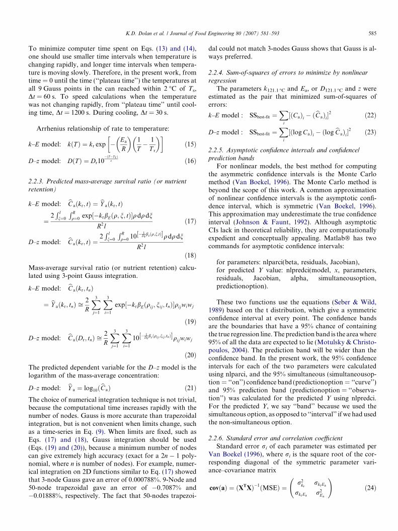
4.1.4. Dependent variable

The 95% confidence bands and 95% prediction bandsfor the survival ratio bY a are shown separately for eachretort temperature (Figs. 2–4). In general, both the confi-dence and prediction bands were smaller at short and longtimes, and reached a maximum at some time in the middle(Fig. 2 shows the trend best). This non-constant size of CBsis common for nonlinear models (Bates & Watts, 1988, pp.59–60). The width of the CBs ranged from 0 to 0.235, whileprediction bands ranged from 0.519 to 0.570. As expected,more than half the points lie outside the CB, while all thepoints lie within the PB (Fig. 2). These plots reveal thepower of using a nonisothermal method over an isothermalmethod, namely, that the rate constant and activation

Fig. 2. Case 1. Welt (1996) data. 95% asymptotic confidence band and 95% p104.4 �C. Prediction curve, confidence band, and prediction bands were const

energy over a large temperature range can be found withfewer experiments. In this case, the temperature range ofthe material in the cans was 0 �C to �120 �C. Covering arange that large with isothermal experiments would be pro-hibitively expensive and time-consuming.

4.2. Case 2


Analogous to Case 1, the D121.1 �C value (inversely pro-portional to rate constant) we estimated was 29% lower(6.31 vs. 8.9 min) than Welt et al. (1997) estimated, whilethe z value was the same (11.36 vs. 11.4 �C).

rediction band for survival ratio for cans heated at retort temperature ofructed by minimizing total sum-of-squares for the data in Figs. 2–4.

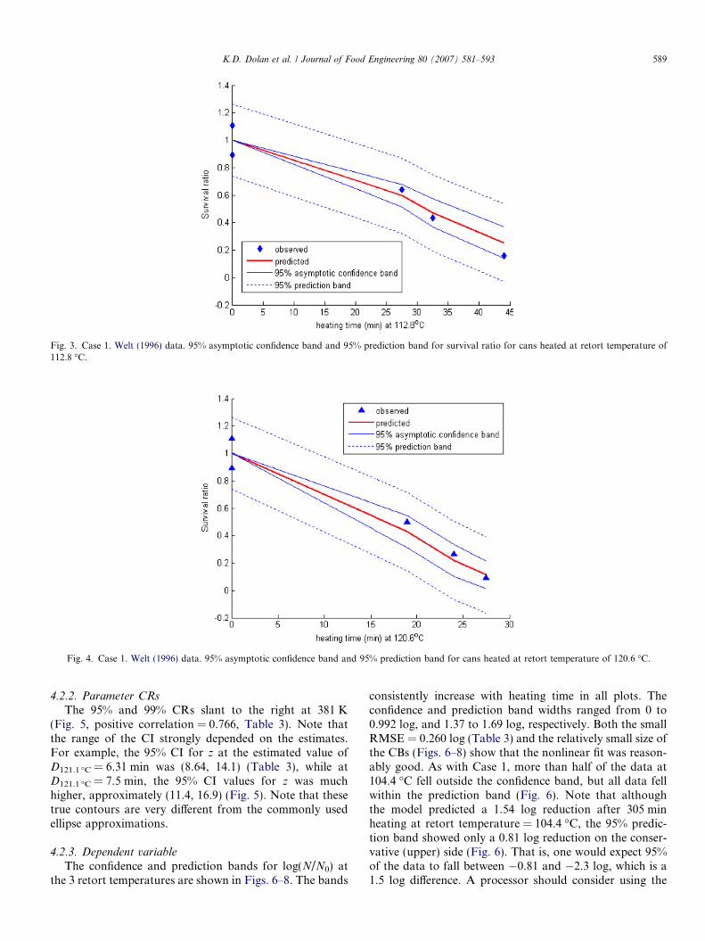
Fig. 3. Case 1. Welt (1996) data. 95% asymptotic confidence band and 95% prediction band for survival ratio for cans heated at retort temperature of112.8 �C.

Fig. 4. Case 1. Welt (1996) data. 95% asymptotic confidence band and 95% prediction band for cans heated at retort temperature of 120.6 �C.


4.2.2. Parameter CRs

The 95% and 99% CRs slant to the right at 381 K(Fig. 5, positive correlation = 0.766, Table 3). Note thatthe range of the CI strongly depended on the estimates.For example, the 95% CI for z at the estimated value ofD121.1 �C = 6.31 min was (8.64, 14.1) (Table 3), while atD121.1 �C = 7.5 min, the 95% CI values for z was muchhigher, approximately (11.4, 16.9) (Fig. 5). Note that thesetrue contours are very different from the commonly usedellipse approximations.

4.2.3. Dependent variableThe confidence and prediction bands for log(N/N0) at

the 3 retort temperatures are shown in Figs. 6–8. The bands

consistently increase with heating time in all plots. Theconfidence and prediction band widths ranged from 0 to0.992 log, and 1.37 to 1.69 log, respectively. Both the smallRMSE = 0.260 log (Table 3) and the relatively small size ofthe CBs (Figs. 6–8) show that the nonlinear fit was reason-ably good. As with Case 1, more than half of the data at104.4 �C fell outside the confidence band, but all data fellwithin the prediction band (Fig. 6). Note that althoughthe model predicted a 1.54 log reduction after 305 minheating at retort temperature = 104.4 �C, the 95% predic-tion band showed only a 0.81 log reduction on the conser-vative (upper) side (Fig. 6). That is, one would expect 95%of the data to fall between �0.81 and �2.3 log, which is a1.5 log difference. A processor should consider using the

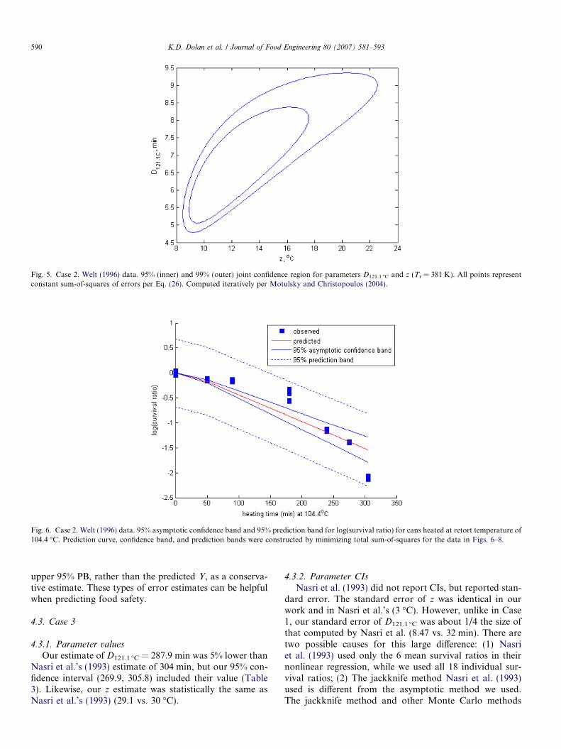
Fig. 5. Case 2. Welt (1996) data. 95% (inner) and 99% (outer) joint confidence region for parameters D121.1 �C and z (Tr = 381 K). All points representconstant sum-of-squares of errors per Eq. (26). Computed iteratively per Motulsky and Christopoulos (2004).

Fig. 6. Case 2. Welt (1996) data. 95% asymptotic confidence band and 95% prediction band for log(survival ratio) for cans heated at retort temperature of104.4 �C. Prediction curve, confidence band, and prediction bands were constructed by minimizing total sum-of-squares for the data in Figs. 6–8.


upper 95% PB, rather than the predicted Y, as a conserva-tive estimate. These types of error estimates can be helpfulwhen predicting food safety.

4.3. Case 3


Our estimate of D121.1 �C = 287.9 min was 5% lower thanNasri et al.’s (1993) estimate of 304 min, but our 95% con-fidence interval (269.9, 305.8) included their value (Table3). Likewise, our z estimate was statistically the same asNasri et al.’s (1993) (29.1 vs. 30 �C).

4.3.2. Parameter CIs

Nasri et al. (1993) did not report CIs, but reported stan-dard error. The standard error of z was identical in ourwork and in Nasri et al.’s (3 �C). However, unlike in Case1, our standard error of D121.1 �C was about 1/4 the size ofthat computed by Nasri et al. (8.47 vs. 32 min). There aretwo possible causes for this large difference: (1) Nasriet al. (1993) used only the 6 mean survival ratios in theirnonlinear regression, while we used all 18 individual sur-vival ratios; (2) The jackknife method Nasri et al. (1993)used is different from the asymptotic method we used.The jackknife method and other Monte Carlo methods

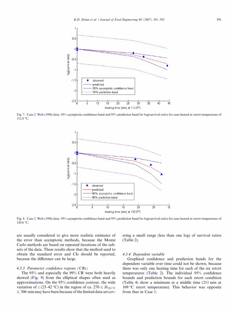
Fig. 7. Case 2. Welt (1996) data. 95% asymptotic confidence band and 95% prediction band for log(survival ratio) for cans heated at retort temperature of112.8 �C.

Fig. 8. Case 2. Welt (1996) data. 95% asymptotic confidence band and 95% prediction band for log(survival ratio) for cans heated at retort temperature of120.6 �C.


are usually considered to give more realistic estimates ofthe error than asymptotic methods, because the MonteCarlo methods are based on repeated iterations of the sub-sets of the data. These results show that the method used toobtain the standard error and CIs should be reported,because the difference can be large.

4.3.3. Parameter confidence regions (CRs)

The 95% and especially the 99% CR were both heavilyskewed (Fig. 9) from the elliptical shapes often used asapproximations. On the 95% confidence contour, the widevariation of z (23–42 �C) in the region of ca. 270 6 D121 �C

6 306 min may have been because of the limited data set cov-

ering a small range (less than one log) of survival ratios(Table 2).

4.3.4. Dependent variable

Graphical confidence and prediction bands for thedependent variable over time could not be shown, becausethere was only one heating time for each of the six retorttemperatures (Table 2). The individual 95% confidencebounds and prediction bounds for each retort condition(Table 4) show a minimum at a middle time (211 min at109 �C retort temperature). This behavior was oppositefrom that in Case 1.

Fig. 9. Case 3. Nasri et al. (1993) data. 95% (inner) and 99% (outer) joint confidence region for parameters D121 �C and z (Tr = 376 K). All points representconstant sum-of-squares of errors per Eq. (26). Computed iteratively per Motulsky and Christopoulos (2004).

Table 4Case 3. Nasri et al. (1993) data

Retort temperature (�C) Heating time (min) Predicted log(retention) 95% confidence band width (log) 95% prediction band with (log)

116 92 �0.139 0.0494 0.1762115 100 �0.145 0.0481 0.1758112 137 �0.177 0.0457 0.1752109 211 �0.239 0.0440 0.1748106 367 �0.354 0.0475 0.1757103 675 �0.535 0.0897 0.1914

95% Confidence intervals and 95% prediction intervals for log(retention) for each of six retort time–temperature conditions.


5. Conclusions

Most literature that reports confidence intervals forkinetic parameters has not reported the confidence inter-val for predicted Y, even though the predicted Y is moreimportant than the estimated parameters for food safetypurposes. In this article, three case studies were exam-ined. The confidence intervals for parameters and theconfidence and prediction intervals for predicted Y werecomputed. Both the k–E and the D–z model were used.Upper 95% prediction bands gave a more conservative(safer) limit than the Y value predicted by the model,up to a 0.84 log difference. This result indicates thatfor food safety considerations, the upper prediction bandis more important than the model prediction (regressionline). Confidence regions for the parameters were some-times highly skewed from the typical elliptical approxi-mations used in most of the literature. The intent ofthis work was to propose a framework for otherresearchers to use when reporting error in kinetic studies.Because this nonlinear regression method is easy to use,and can be implemented conveniently using Matlab� orVisual Basic for Applications on Excel�, we hope thatresearchers will use the method on other data to disproveor confirm our results.

Acknowledgements

We thank Dr. Bradley Marks for helpful comments inpreparing this manuscript. This research has been sup-ported in part by NSF grant DMS0405330.

References

Bates, D. M., & Watts, D. G. (1988). Nonlinear regression analysis and its

application. New York: Wiley.Carslaw, H. S., & Jaeger, J. C. (1959). Conduction of heat in solids (second

ed.). Oxford London: Oxford University Press.Claeys, W. L., Ludikhuyze, L. R., & Hendrickx, M. E. (2001). Formation

kinetics of hydroxymethylfurfural, lactulose, and furosine in milkheated under isothermal and non-isothermal conditions. Journal of

Dairy Research, 68, 287–301.Claeys, W. L., Ludikhuyze, L. R., van Loey, A. M., & Hendrickx, M. E.

(2001). Inactivation kinetics of alkaline phosphatase and lactoperox-idase, and denaturation kinetics of b-lactoglobulin in raw milk underisothermal and dynamic temperature conditions. Journal of Dairy

Research, 68, 95–107.Dolan, K. D., Steffe, J. F., & Morgan, R. G. (1989). Back extrusion and

simulation of viscosity development during starch gelatinization.Journal of Food Processing Engineering, 11, 79–101.

Fernandez, A., Ocio, M. J., Fernandez, P. S., Rodrigo, M., & Martinez, A.(1999). Application of nonlinear regression analysis to the estimationof kinetic parameters for two enterotoxigenic strains of Bacillus cereus

spores. Food Microbiology, 16(6), 607–613.


Fernandez, A., Ocio, M. J., Fernandez, P. S., Rodrigo, M., & Martinez, A.(2001). Effect of heat activation and inactivation conditions ongermination and thermal resistance parameters of Bacillus cereus

spores. International Journal of Food Microbiology, 63, 257–264.Johnson, M. L., & Faunt, L. M. (1992). Parameter estimation by least-

squares methods. Methods in Enzymology, 210, 25.Lenz, M. K., & Lund, D. B. (1977a). The lethality-Fourier number

method: experimental verification of a model for calculating temper-ature profiles and lethality in conduction-heating canned foods.Journal of Food Science, 42(4), 989–996, 1001.

Lenz, M. K., & Lund, D. B. (1977b). The lethality-Fourier numbermethod: confidence intervals for calculated lethality and mass-averageretention of conduction-heating, canned foods. Journal of Food

Science, 42(4), 1002–1007.Lenz, M. K., & Lund, D. B. (1980). Experimental procedures for

determining destruction kinetics of food components. Food Technol-

ogy, 34(2), 51–55.Motulsky, H. J., & Christopoulos, A. (2004). Fitting models to biological

data using linear and nonlinear regression. A practical guide to curve

fitting. New York, NY: Oxford University Press, pp. 110–117.

Myers, G. E. (1971). Analytical methods in conduction heat transfer. NewYork: McGraw-Hill.

Nasri, H., Simpson, R., Bouzas, J., & Torres, J. A. (1993). An unsteady-state method to determine kinetic parameters for heat inactivation ofquality factors: conduction-heated foods. Journal of Food Engineering,

19, 291–301.Seber, G. A. F., & Wild, C. J. (1989). Nonlinear regression. NY: John

Wiley & Sons, pp. 191–193.van Boekel, M. A. J. S. (1996). Statistical aspects of kinetic modeling for

food science problems. Journal of Food Science, 61(3), 477–489.van den Hout, R., Meerdink, G., & Van’t Riet, K. (1999). Modelling of

the inactivation kinetics of the trypsin inhibitors in soy flour. Journal of

the Science of Food and Agriculture, 79(1), 63–70.Welt, B. A. (1996). Kinetic parameter estimation in prepackaged foods

subjected to dynamic thermal treatments, Ph.D. thesis, University ofFlorida, Gainesville, FL.

Welt, B. A., Teixeira, A. A., Balaban, M. O., Smerage, G. H., Hintinlang,D. E., & Smittle, B. J. (1997). Kinetic parameter estimation inconduction heating foods subjected to dynamic thermal treatments.Journal of Food Science, 62(3), 529–534, 538.

nonlinear regression technique to estimate kinetic...

Documents