nonlinear oscillations and multiscale dynamics …

.

NONLINEAR OSCILLATIONS AND MULTISCALE DYNAMICS IN A

CLOSED CHEMICAL REACTION SYSTEM

YONGFENG LI, HONG QIAN, AND YINGFEI YI

Abstract. We investigate the oscillatory chemical dynamics in a closed isothermal reaction sys-tem described by the reversible Lotka-Volterra model. This is a three-dimensional, dissipative,singular perturbation to the conservative Lotka-Volterra model, with the free energy serving asa global Lyapunov function. We will show that there is a natural distinction between oscillatoryand non-oscillatory regions in the phase space, that is, while orbits ultimately reach the equi-librium in a non-oscillatory fashion, they exhibit damped, oscillatory behaviors as interestingtransient dynamics.

1. Introduction

Since the discovery of the Belousov-Zhabotinsky (BZ) reaction and the “Oregonator” mechanism([5, 24, 31]), many new studies in cell biology have also indicated the importance of chemicaloscillations and it is well-believed that these oscillations can emerge as the collective dynamicbehavior of interacting components in the cell. But little understanding is known about themechanisms and underlying principles of such oscillations, for which modeling and analysis areessential ([16]).

There are essentially two types of reaction systems in which chemical oscillations can be observed.One is open system where exchange of matter and/or energy with the surroundings is allowed,and the other is closed system without such exchange. Following the pioneer work of Belousov-Zhabotinsky, open systems have been widely studied for the understanding chemical oscillations(see [11, 13, 21, 22, 24, 26] and references therein) and related dynamical issues (see e.g., [12] forcomposite double oscillations, [7] for the existence of limit cycles, [29] for chaos, [4, 14, 15] forwave motions, and [20, 30, 32] for period-doubling bifurcations). To the contrary, little is knownabout the nature of chemical oscillations in a closed system. While sustained oscillations aretypically observed in an open system, the reaction in a closed system should go to the equilibriumstate ([25]) and yield transitory, quasi-stationary oscillation ([5]) according to the laws of non-equilibrium thermodynamics ([3]). In fact, our recent work [19] on a reversible Lotka-Volterra(LV) reaction system has shown that chemical oscillations in a closed system exhibit a uniquedynamical behavior differing from that of the traditionally studied nonlinear oscillations arising inmechanical and electrical systems.

2000 Mathematics Subject Classification. Primary 34C15, 34E15, 37L45, 92E20.Key words and phrases. Closed chemical reaction, Reversible Lotka-Volterra system, Multi-scale dynamics,

Nonlinear oscillation, Singular perturbation.Dedicated to Professor Jack K. Hale on the occasion of his 80th birthday.The first author was partially supported by the Institute for Mathematics and its Applications and the third

author was partially supported by NSF grant DMS0708331, NSFC Grant 10428101, and a Changjiang Scholarshipfrom Jilin University.

1

2 Y.-F. LI, H. QIAN and Y. YI

The present paper is a continuation of our previous study in [19] on reversible Lotka-Volterra(LV) reaction system in which detailed dynamical behaviors of the underlying chemical oscillationswill be analyzed. More precisely, consider the reversible Lotka-Volterra (LV) reaction

(1.1) A+Xk1

⇌

k−1

2X, X + Yk2

⇌

k−2

2Y, Yk3

⇌

k−3

B,

where X , Y , A and B denote the concentrations of the four species in the chemical reaction, k1,k2 and k3 are forward reaction rates and k−1, k−2 and k−3 are reverse reaction rates. The law ofmass action then yields the following differential equations

(1.2)

⎧

⎨

⎩

dx

dt= k1cAx− k−1x

2 − k2xy + k−2y2,

dy

dt= k2xy − k−2y

2 − k3y + k−3cB,

dcA

dt= −k1cAx+ k−1x

2,

dcB

dt= k3y − k−3cB

on the concentration rates x, y, cA, cB of X,Y,A,B respectively. Under the rescaling

(1.3)u = k2

k3x, v = k2

k3y, w = k1

k3cA, z = k2

k3cB,

� = k3t, " = k−1

k1= k−2

k2= k−3

k3, � = k1

k2.

the system (1.2) has the following dimensionless form

(1.4)

⎧

⎨

⎩

du

d�= u(w − v)− "(�u2 − v2),

dv

d�= v(u− 1)− "v2 + "z,

dw

d�= −�(wu − "�u2),

dz

d�= v − "z.

We assume that the backward reaction is much slower than the forward reaction and the firstforward reaction is slower than the second forward reaction, and the ratios � and " satisfy 0 < " ≪� ≪ 1. Using the conservation of total concentration � = u + v + w

�+ z, system (1.4) is further

reduced into the following three-dimensional system

(1.5)

⎧

⎨

⎩

du

d�= u(w − v)− "(�u2 − v2),

dv

d�= v(u− 1)− "v2 + "

(

� − u− v − w�

)

,

dw

d�= −�(wu − "�u2).

The system (1.5) is dissipative, and, in fact, a two-scale singular perturbation of Hamiltoniansystems. As " = � = 0, the unperturbed systems become a family of standard conservative LVsystems which bear Hamiltonian structures by appropriate transformations. Each unperturbedsystem admits a family of periodic solutions with distinct frequencies. But when the perturbationis tuned on, dissipation will eliminate all periodic motions. Instead, as what we will show, thesystem (1.5) admits a unique globally attracting equilibrium, and moreover, the attraction is non-oscillatory in a non-oscillating zone near the equilibrium, simply because the equilibrium is anasymptotically stable node. Still, away from the equilibrium, we will also show that there isan oscillating zone in which solutions will oscillate in the (u, v)-direction around a central axiswhile moving downward in the w-direction, with decreasing oscillating diameters in response tothe damping. In fact, each round of oscillation around the central axis consists of two parts: a“horizontal” portion with nearly unchanged energy and w-value which shadows a periodic orbit

NONLINEAR OSCILLATION IN REVERSIBLE LV SYSTEM 3

of the unperturbed system on the same energy level, and a “vertical” portion with exponentiallydecay energy and w-values. Such an oscillatory phenomenon well fits in the physical intuitionpredicted by the Second Law of Thermodynamics that chemical oscillation is far away from theequilibrium and the reaction eventually approaches the chemical equilibrium state as free energydissipates.

The system (1.5) is also interesting from a pure dynamics point of view. First of all, it isa dissipative perturbation to conservative systems. This is an area for which little is known indynamical systems theory. The second, for such a system, although long term dynamics are simple,the transient, finite-time ones are of the most theoretical and physical interests. We remark thatthough there have been many studies in transient dynamics such as chaos and nonlinear waves([1], [2], [8], [9], [18], [23], [28]), transient oscillations have not been much explored in dynamicalsystems theory besides the short-lived ones arising in electrical and mechanical systems due tosudden changes of voltage, current, or load. Finally, each orbit in the system admits a mixture ofconservative, dissipative, and monotone natures, corresponding to the shadowing of conservativeoscillations, jumping due to dissipation, and non-oscillatory convergence, respectively. This is alsoa new phenomenon in dynamical systems theory.

Detailed contents of the paper is as follows. Section 2 is devoted for the description of generalglobal dynamics of (1.5), in which we show the dissipative property of the system and globalattraction of the equilibrium. In Section 3, we use the integral manifolds theory and Poincaremaps to describe oscillations away from the equilibrium in the oscillating zone by considering theexistence of central axis and nature of oscillations. In Section 4, we apply the geometric theory ofsingular perturbations to describe the nature of convergence in the non-oscillating zone near theequilibrium. Some discussions on transit dynamics in the transition zone in between the oscillatingand the non-oscillating zones will be made in Section 5.

2. Global Dynamics

In this section, we will consider the general global dynamics of the reversible LV system (1.5).Because each state variable in system (1.5) represents the concentration of the respective chemicalreactant, it only makes sense that each variable remains positive during the time evolution. Thiscan be shown by applying the invariance principle due to LaSalle([17]) and Hale([10]) to constructan invariant set in the first octant ℝ3+. Meanwhile the long time behavior of system (1.5) can bealso determined consequently.

For any fixed � > 1, define a tetrahedron

T ={

(u, v, w) ∈ ℝ3, u, v, w ≥ 0, and u+ v +

w

�≤ �}

and let P∗ = (u∗, v∗, w∗)⊤ ∈ T , where

u∗ ="2�

r("), v∗ =

"�

r("), w∗ =

�"3�

r("), r(") = 1 + "+ "2 + "3.

Theorem 2.1. System (1.5) is dissipative and allows a positively invariant set given by T in whichP∗ is a global attractor of (1.5).


Proof. To show the dissipative property, we trace back to the original four-dimensional system(1.4). Denote by F (X) the vector field on the right hand side of (1.4) with X = (u, v, w, z) and

z∗ = � − u∗ − v∗ − w∗

�= �

r(") for given � > 1. Define

L(X) = u ln( u

u∗

)

+ v ln( v

v∗

)

+w

�ln( w

w∗

)

+ z ln( z

z∗

)

,

thend

d�L(X) =

⟨

∇L(X),dX

d�

⟩

= uwp("�u

w

)

+ uvp("v

u

)

+ vp("z

v

)

,

where p(x) = (1−x) lnx ≤ 0 for all x > 0 and p(x) = 0 if and only if x = 1. Therefored

d�L(X) ≤ 0

for all X ∈ ℝ4+. Note that in X ∈ ℝ

4+,d

d�L(X) = 0 if and only if

p("�u

w

)

= p("v

u

)

= p("z

v

)

= 0 ⇐⇒ "�u

w=

"v

u=

"z

v= 1,

or, w = �"u, u = "v, v = "z, which, under the constraint u + v + w�+ z = � yields that u = u∗,

v = v∗, w = w∗ and z = z∗. Hence L(u, v, w, �−u−v− w�) plays the role of Lyapunov function for

system (1.5) and by the invariance principle due to LaSalle and Hale ([17, 10]), T is a positivelyinvariant set and P∗ is a global attractor of system (1.5) and hence (1.5) is dissipative. Thiscompletes the proof. 2

Theorem 2.1 says that the long term dynamics of system (1.5) is simple. And because of theinvariance, T is called reaction zone and all the further analysis will be carried out in T .

Moreover, we remark that the Lyapunov function L is precisely the free energy in thermody-namics. Thus the conclusion of the theorem above agrees with the second Law of Thermodynamicsthat the free energy must be decreasing to reach its minimum. However, because system (1.5) isnot a gradient system, at least not the gradient of L, the solution curve does not go along withthe direction of −∇L, i.e., the reaction in our system does not proceed along the deepest decentdirection of the free energy. It is interesting to point out that, from chemistry point of view, ourresults clearly show that the chemical dynamics does not follow the gradient descent of the freeenergy function. We believe this is a rather deep theoretical physics problem whose origin remainsto be explained.

3. Oscillating Zone

Although each orbit of (1.5) in T ultimately reaches the equilibrium P∗, we will show in thissection that there is an oscillating zone away from the equilibrium in which all solutions oscillatearound a central axis.

3.1. Central Axis. In the case " = 0, the system (1.5) reduces to the following partially perturbedsystem

(3.1)

⎧

⎨

⎩

du

d�= u(w − v),

dv

d�= v(u− 1),

dw

d�= −�uw.

It is easy to see thatW o

� = {(u, v, w), u = ��, v = w} ,


where �� = 11+�

, is an one-dimensional, asymptotically stable, invariant manifold of (3.1) on which

v = w ∼ e−��t. As " is a regular perturbation parameter, our next theorem shows that a similarinvariant curve exists for the full system (1.5).

Theorem 3.1. Away from the equilibrium, there exists an one-dimensional asymptotically stable,smooth, locally invariant manifold W o

�," with the following properties:

a) For fixed � ≪ 1,

W o�," = {(u, v, w) ∈ T : u = �� + "f1(w) +O("2),

v = w + "g1(w) +O("2), w ≥ �2},where

f1 = �

[

−f11

∫

f12(w)p(w)dw + f12

∫

f11(w)p(w)dw

]

,

g1 = ��w

[

−f ′11

∫

f12(w)p(w)dw + f ′12

∫

f11(w)p(w)dw

]

− �� +w2

��

,

with p(w) = c2 +c3w

+ c4w2 , f11 =

√wJ1(2

√c1w) and f12 =

√wY1(2

√c1w), and J1 and Y1

being the Bessel’s functions of first and second kinds, respectively, and

c1 =

(

1 + �

�

)2

, c2 =1− �2

�2, c3 =

(1 + �)2

�3, c4 =

1+ �

�2(� − ��).

b) Each solution on W o�," decays exponentially with rate ∼ ��.

Proof. We note that under the transformation

u → x+ ��, v → y + w, w → w,

the system (1.5) becomes

(3.2)

{

dXd�

= A�(w)X +G(X,w, �, ")dwd�

= �F (X,w, �, ")

where

A�(w) =

[

0 −��

(1 + �)w −��

]

, F (X,w, �, ") = −(x+ ��) [w − "�(x+ ��)] ,

G(X,w, �, ") =

[

−xy − "�(x+ ��)2 + "(y + w)2

xy − "[

�2(x+ ��)2 + (y + w)2 + (x+ ��) + (y + w) + w

�− �

]

]

.

As w ≥ �2�2�

4 , A�(w) has two complex eigenvalues with negative real parts −��

2 and hence the

freezed system dXd�

= A�(w)X is uniformly exponentially stable with exponent � = ��

2 . For each s,we denote by Φ�(�, s, w) the fundamental matrix of this freezed system with Φ�(s, s, w) =Identity.

Let f be a smooth cutoff function such that f(w) = 1 for w ∈ I = [�2, ��], f(w) = 0 for

w ∈ (0,�2�2

�

4 ] and w ∈ (�� + 1,∞), 0 ≤ f(w) ≤ 1 and ∣f ′(w)∣ ≤ 2. Define

F (X,w, �) = F (X,w, �)f(w)

and consider the modified system

(3.3)

{

dXd�

= A�(w)X +G(X,w, �, ")dwd�

= �F (X,w, �, ").

We note that for fixed � ≪ 1, " introduces a regular perturbation when w ≥ �2, and G =O(∣X ∣2 + "). It is then easy to see that the proof in [27, 34] for the existence, asymptotic stability,and smoothness of integral manifolds holds true for system (3.3), yielding an one-dimensional,

smooth, asymptotically stable, invariant manifold W�," for (3.3). In fact, for any continuous


function X(�), let w = W (w0, X)(�) denote the solution of the second equation of (3.3) withinitial value w0 ∈ I. Then it follows from the proof in [27, 34] that there exists a sufficiently smallconstant "1 > 0 such that the mapping

ℱ(X)(�) =

∫ �

−∞Φ�(�, s,W (w0, X)(s))G(X,W (w0, X)(s), s)ds

is well defined in an appropriate function space containing {∣X ∣ < "1}, and is also a uniformlycontraction mapping. Moreover, if X(�) is the fixed point, then the graph of X(w0, �, ") = X(0)

defines the invariant manifold W�,". In vitro of the cutoff function and by replacing w0 by w, it isnow clear that

W o�," =

{

(u, v, w) ∈ W�,", w ∈ I}

is the desired one-dimensional, locally invariant manifold for system (3.2).

To prove a), we use the fact that " is a regular perturbation parameter and expand X(w, �, "),for fixed �, into the following Taylor series

u = �� +

∞∑

k=1

fk(w)"k, v = w +

∞∑

k=1

gk(w)"k.

Since W o�," is the graph of X(w, �, "), a) is then proved by substituting the Taylor series into (1.5)

and comparing the coefficients.

As the restricted equation on W o�," is a regular perturbation of that on W o

� , b) follows from theexponential decay property of solutions on W o

� . 2

3.2. Oscillatory Behavior. Let �t denote the flow induced by system (1.5) and B�

(

W o�,"

)

be a�-neighborhood of W o

�,". With 0 < " ≪ � ≪ 1 fixed, for certain 1 < � < 2 determined by � and ",we refer the set

T o = T∩

⎛

⎝

∪

t≤0

�t

(

B�

(

W o�,"

))

⎞

⎠

∩

{(u, v, w) ∈ T : w ≥ ��}

as the oscillating zone, where � ∼ (� − 2)�� ln�. From the construction of W o�," in the proof of

Theorem 3.1, we see that as w ≥ �2�2�

4 , the linearized matrix A�(w) has two complex eigenvalueswith negative real parts. This suggests the possibility of oscillations around the central axis W o

� .In fact, as described in the theorem below, oscillations around the central axis exhibit both regularand singular behaviors.

Let

T o1 = {(u, v, w) ∈ T : w ≥ �} ,

T o2 =

{

(u, v, w) ∈ T : w ≥ �2}

,

Ω− = {(u, v, w) ∈ T : v < w} ,Ω+ = {(u, v, w) ∈ T : v > w} .

As we will see below, Ω+ ∩ Ω− plays the role of a Poincare section and the number of oscillations

for each orbit in T o can be measured by counting its number of returns to the section.

Theorem 3.2. There exists an � = �(", �) ∈ (1, 2) such that the following holds as " ≪ � ≪ 1.

a) T o1 ⊂ T o ⊂ T o

2 .


b) Each orbit starting in T o oscillates a finite number of times around the central axis W o�,",

with decreasing distance to the axis, and moreover, there is a constant c0 > ��−1 suchthat, the oscillation number of each orbit with initial energy E�

0 and initial w0 = c0� isless than −c0(�− 1) ln�

��E�0

.

c) Each round of oscillation around W o�," consists of two parts: a “horizontal” portion in Ω+

with nearly unchanged energy and w-value which shadows a periodic orbit of the unperturbedsystem(where " = � = 0) on the same energy level, and a “vertical” portion in Ω− withexponentially decaying energy and w-values.

d) There is a constant c > 0 such that at the bottom of the oscillating zone T o where w ∼ ��,the energy E� is less than or equal to c(�− 2)�� ln�.

Proof. Since w is monotonically decreasing when w ≥ �"�, part a) of the theorem follows from thedefinition of T o and the construction of W o

� in the proof of Theorem 3.1.

As " is a regular perturbation parameter, it is sufficient to prove the remaining parts of thetheorem for the partially perturbed system (3.1). Consider the following transformation

(1 + �)[

(u− ��) + �� ln(��

u

)]

= E� cos2 �,

(v − w) + w ln(w

v

)

= E� sin2 �,

where � is the (counterclockwise) rotation angle around W o� = {(u, v, w), u = ��, v = w} which

is an approximation of W o�,", and E� is the translated total free energy for the partially perturbed

system (3.1) which is proportional to the distance to W o� . Under this transformation the system

(3.1) becomes

(3.4)

⎧

⎨

⎩

E� = −�uE� sin2 �,w = −�uw,

� = Θ�(E�, w, �),

where

Θ�(E�, w, �) =

⎧

⎨

⎩

(−1)k(1 + �)(u − ��)

√w√

2E�, � = k�;

(−1)k(1 + �)(v − w)√

2E�, � = k� + �

2 ;

(1 + �)

2E�

(

u− ��

cos �

)(

v − w

sin �

)

− �u

2sin � cos �, otherwise.

Clearly, E� ≤ 0.

Consider the Poincare section Σ� = {(u, v, w), u > 0, u ∕= ��, v = w ≥ ��} and let

Σ�+ = {(u, v, w) ∈ Σ�, u > ��}, Σ�

− = {(u, v, w) ∈ Σ�, 0 < u < ��}.It is easy to see that the flow ��

t generated from the partially perturbed system (3.1) crosses Σtransversely except when u = ��, and, those starting from Σ+ (resp. Σ−) will travel in Ω+ (resp.Ω−) then reach Σ− (resp. Σ+). Let � : Σ� → Σ�: P 7→ �t(P )(P ), be the Poincare map, wheret(P ) is the first return time.

From the definition of Θ�, it is easy to see that � ≥ c > 0 as w > � where c depends on � andE�

0 . Hence each orbit starting in T o1 oscillates around W o

� . Starting from a P0 ∈ Σ�+ ∩ T o

1 , weconsider a sequence of points {Pn = (E�

n , wn, �n)} ⊂ T o such that Pn+1 = �(Pn), n = 0, 1, ⋅ ⋅ ⋅ .


For each n, write wn = cn�. Then cn > ��−1, and in particular, cn = O(1) if Pn ∈ T o1 . Denote

tn = t(Pn), n = 0, 1, ⋅ ⋅ ⋅ . Since[

ln(vw1� )]′

=v

v+

1

�

w

w= (u− 1)− u = −1,

we have

(3.5) tn = ln(

vnw1�n

)

− ln(

vn+1w1�

n+1

)

=1

��

(lnwn − lnwn+1) .

We now consider in the above sequence three consecutive points P2k, P2k+1, P2k+2. ThenP2k, P2k+2 ∈ Σ+ and P2k+1 ∈ Σ−. We note that Θ� can be rewritten as

Θ� =

(

u− ��

2 cos �

)[(

v − w

E� sin �

)

+ �

(

w ln vw

E� sin �+ sin3 �

)]

− ��

2sin � cos �.

Let (u(t), v(t), w(t)) be the portion of the orbit from P2k to P2k+2. Since bothu− ��

cos �> 0 and

v − w

sin �> 0 and

v − w√E� sin �

≥√

2w2k+1 as � ∈ [2k�, (2k+1)�], there exists a constant c∗ such that

(3.6) Θ� > c∗√

2w2k+1 −�

4> 0.

It follows that

t2k =

∫ (2k+1)�

2k�

1

Θ�

d� <4�

4c∗√2w2k+1 − �

.

Hence by (3.5),

1 <w2k

w2k+1= e��t2k < exp

(

4��√�

4c∗√2c2k+1 −

√�

)

∼ 1,

i.e., w2k+1 = (1 +O(�1− �2 ))w2k. From the first two equation in (3.4), we also have

dE�

dw=

E�

wsin2 � ≤ E�

w,

which implies that

1 >E�

2k+1

E�2k

≥ w2k+1

w2k∼ 1.

Hence E�2k+1 = (1 +O(�1− �

2 ))E�2k. From the monotonicity of E� and w, we also see that for this

portion of the orbit, E� and w remain near constants, for which the last equation of the system(3.4) becomes a regular perturbation to the corresponding one in the unperturbed system (i.e.,when � = 0 in (3.4)). It follows that this portion of the orbit shadows the (periodic) solution ofthe unperturbed system with the same initial value (see e.g., [33]).

On the other hand, as � ∈ [(2k + 1)�, (2k + 2)�], we have v ≤ w ≤ w2k+1. Then

t2k+1 =

∫ u2k+2

u2k+1

1

u(w − v)du >

∫ u2k+2

u2k+1

1

uwdu >

∫ u2k+2

u2k+1

1

uw2k+1du =

1

w2k+1ln

u2k+2

u2k+1.

Since u2k+1 < ��e−E�

2k+1 and u2k+2 > ��, we have

w2k+2

w2k+1= e−��t2k+1 <

(

u2k+2

u2k+1

)− ��w2k+1

< exp

(

−��E

�2k+1

w2k+1

)

.

Butd

dt

(

E�

w

)

=E�w − E�w

w2=

−�uE�w sin2 � + �uE�w

w2= �u cos2 �

E�

w≥ 0,


i.e., E�

wis increasing in time. Thus,

(3.7)w2k+2

w2k+1< exp

(

−��E�0

w0

)

= exp

(

−��E�0

c0

)

.

To estimate E2k+2

E2k+1, we let

Θ� =Θ�

u= p(�)q(�) − �

2sin � cos �,

where

p(�) =v − w√2E� sin �

=√w

1− vw

√

2E�

w∣ sin �∣

, q(�) =1− ��

u√2E� cos �

.

Then

ln

(

E�2k+2

E�2k+1

)

= −�

∫ (2k+2)�

(2k+1)�

sin2 �

Θ�

d�.

As � ∈ [(2k+1)�, (2k+ 32 )�], since both

E�

wand ∣ sin �∣ are increasing, p(�) is decreasing. While

as � ∈ [(2k + 32 )�, 2(k + 1)�],

d

d�

(

E�

wsin2 �

)

=E�

w

(

2 +�u sin � cos �

Θ�

)

sin � cos � ≤ 0,

i.e., p is increasing. Thus for � ∈ [(2k + 1)�, (2k + 2)�],

p(�) ≤ max{p((2k + 1)�), p(2(k + 1)�)} = max{√w2k+1,√w2(k+1)} ≤ √

w2k+1.

Similarly, q(�) is decreasing for � ∈ [(2k+1)�, (2k+2)�]. Using the fact that if f(x) = x−1−lnx =

a2 with x < 1 then x ≥ e−1−a2

, we have

q(�) ≤��

u2k+1− 1

√

2E�2k+1

≤ e1+E�2k+1 − 1

√

2E�2k+1

.

It follows that as � ∈ [(2k + 1)�, (2k + 2)�],

Θ� ≤ (1 + �)(

e1+E�2k+1 − 1

)

√

w2k+1

2E2k+1+

�

4≤ (1 + �)

(

e1+E�0 − 1

)

√

w0

2E0+

�

4.

Consequently,

ln

(

E�2k+2

E�2k+1

)

≤ −2��

4 (e1+E�0 − 1)

√

w0

2E�0

+ ��

,

or equivalently,

E�2k+2

E�2k+1

≤ exp

⎛

⎝

−2��

4 (e1+E�0 − 1)

√

w0

2E�0

+ ��

⎞

⎠ .

This inequality shows that if w0

E0∼ �2, then the decay rate of the energy E� will be more or less

a constant independent of �, resulting a jump of energy during the second half of each oscillation.

However, if w0

E0∼ �� with 0 < � < 2, then the decay rate will be in the order exp

(

−�1− �2

)

,

resulting only a small jump of energy. The proof of c) is now complete.

It also follows from (3.7) that

w2n

w0=

n∏

k=1

w2k

w2k−2<

n∏

k=1

w2k

w2k−1< exp

(

−n��E�0

c0

)

,


and consequently

n <c0 ln

(

w0

w2n

)

��E�0

.

We note that n is precisely the number of oscillations of the orbit ��t (P0) ending at P2n around the

central axis. We note that if P2n reaches the bottom of the oscillating zone T o, then w2n ≥ ��,from which b) easily follows.

By the inequality Θ� ≥ c∗√2w2n−1 − �

4 as � ∈ [2(n − 1)�, (2n − 1)�], we know that Θ� > 0,

that is, the oscillation proceeds in Ω+∩T o2 . While if � ∈ [(2n− 1)�, 2n�], then we have v−w√

E� sin �≥

√2v ≥

√

2v2n− 12and Θ� ≥ c∗

√

2v2n− 12− �

4 , where v2n− 12, w2n− 1

2and E�

2n− 12

(associated to

� = 2n� − �2 ) satisfy

v2n− 12− w2n− 1

2− w2n− 1

2ln

(

v2n− 12

w2n− 12

)

= E�2n− 1

2

and hence

v2n− 12< w2n− 1

2exp

(

−E�

2n− 12

w2n− 12

)

< w2n−1 exp

(

−E�2n−1

w2n−1

)

.

To proceed the oscillation to reach P2n which is close to the bottom of the oscillation zone T o, itis necessary that Θ� > 0 for which it is sufficient to have

�2

32c2∗≤ v2n− 1

2< w2n−1 exp

(

−E�2n−1

w2n−1

)

or

E�2n < E�

2n−1 ≤ w2n−1 ln

(

32c2∗w2n−1

�2

)

∼ (�− 2)�� ln�.

2

According to numerical simulations, it seems that for two orbits initiated in Ω+ ∩ T o1 with the

same w-initial value, the one with smaller initial distance to W o�," has a less number of oscillations

around it in T o. As the number of jumps made by an orbit in T o is approximately equal to itsnumber of oscillations, a possible mechanism behind this could be that the one with smaller initialdistance to W o

�," would have bigger total length of jumps in T o (hence a less number of jumpswhich would imply a less number of total oscillations). Indeed, by the estimate (3.7), this is truefor the first jumps made by the two orbits.

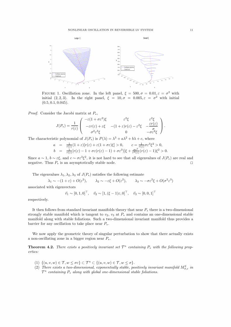
The above theorem is stated for a fixed �. If we allow � to depend on � in the scale of 1�, then

w = O(1) can be considered. In this case, it is not hard to see that � can be also treated as aregular parameter, and hence all oscillations in the oscillating zone are regular without significantjumps in w-values. The numerical plugs in Figure 1 below give comparisons between the regularand singular oscillatory behaviors.

4. Non-oscillating Zone

In this section, we show the existence of a non-oscillating zone near the the equilibrium andstudy its dynamical behaviors.

Theorem 4.1. The unique interior equilibrium point P∗ is an asymptotically stable node.


00.5

11.5

22.5

01

23

45

60

0.5

1

1.5

2

2.5

3

3.5

u

Large ξ

v

w

Oscillatory trajectoryCentral axis

0.40.6

0.81

1.21.4

1.61.8

2

00.05

0.10.15

0.20.25

0.30.35

0

0.005

0.01

0.015

0.02

0.025

0.03

0.035

0.04

0.045

u

Small ξ

v

w

Oscillatory trajectoryCentral axis

Figure 1. Oscillation zone. In the left panel, � = 500, � = 0.01, " = �2 withinitial (2, 2, 3). In the right panel, � = 10, � = 0.005, " = �2 with initial(0.5, 0.1, 0.045).

Proof. Consider the Jacobi matrix at P∗,

J(P∗) =1

r(")

⎛

⎜

⎝

−"(1 + �"2)� "2� "2�

−"r(") + "� −(1 + ")r(")− "2� −"r(")

��2"3� 0 −�"2�

⎞

⎟

⎠.

The characteristic polynomial of J(P∗) is P (�) = �3 + a�2 + b�+ c, where

a = 1r(") (1 + ")[r(") + "(1 + �")�] > 0, c = 1

r(")�"3�2 > 0,

b = 1r(") [r(")− 1 + �"(r(") − 1) + �"3)]� + �"2

r2(") (r(") − 1)�2 > 0.

Since a ∼ 1, b ∼ "�, and c ∼ �"3�2, it is not hard to see that all eigenvalues of J(P∗) are real andnegative. Thus P∗ is an asymptotically stable node. 2

The eigenvalues �1, �2, �3 of J(P∗) satisfies the following estimate

�1 ∼ −(1 + ") +O("2), �2 ∼ −"� +O("2), �3 ∼ −�"2� +O(�2"3)

associated with eigenvectors

v1 ∼ [0, 1, 0]⊤, v2 ∼ [1, (� − 1)", 0]⊤, v3 ∼ [0, 0, 1]⊤

respectively.

It then follows from standard invariant manifolds theory that near P∗ there is a two-dimensionalstrongly stable manifold which is tangent to v2, v3 at P∗ and contains an one-dimensional stablemanifold along with stable foliations. Such a two-dimensional invariant manifold thus provides abarrier for any oscillation to take place near P∗.

We now apply the geometric theory of singular perturbation to show that there actually existsa non-oscillating zone in a bigger region near P∗.

Theorem 4.2. There exists a positively invariant set T n containing P∗ with the following prop-erties:

(1) {(u, v, w) ∈ T , w ≤ �"} ⊂ T n ⊂ {(u, v, w) ∈ T , w ≤ �}.(2) There exists a two-dimensional, exponentially stable, positively invariant manifold M2

�," inT n containing P∗ along with global one-dimensional stable foliations.


(3) On M2�,", there exists an one-dimensional, exponentially stable, positively invariant mani-

fold M1�," containing P∗ along with global one-dimensional stable foliations.

Proof. In vitro of Theorem 3.2, we consider the following rescaling

(4.1) u → u, v → "v, w → �"w,

by which equation (1.5) becomes

(4.2)

⎧

⎨

⎩

du

d�= "

[

u(�w − v)− (�u2 − "2v2)]

,

dv

d�= v(u− 1)− "2v2 + (� − u− "v − "w) ,

dw

d�= −�u(w − u).

When � = 0 (hence " = 0), system (4.2) has a two-dimensional reduced manifold

M�0 =

{

(u, v, w), v = ℎ0(u,w) =� − u

1− u, u, w ∈ [0, �]

}

for some fixed � < 1, consisting of equilibria, which is normally, exponentially stable.

By employing a cutoff function near the boundary ∂M�0 , we have by the geometric theory

of singular perturbation ([6]) that under the perturbation M�0 gives rise to a slightly deformed,

two-dimensional, normally exponentially stable, positively invariant manifold

M2�," = {(u, v, w), v = ℎ�,"(u,w), u, w ∈ [0, �]} ,

where ℎ�,"(u,w) = ℎ0(u,w)+O(�). Since the existence of global attractor P∗ implies that there isno periodic orbit in T , the compact invariant manifold M2

�," must contain at least one equilibrium

point. In fact, it is easy to see that P∗ is the only equilibrium contained in M2�,". The geomet-

ric theory of singular perturbations also asserts the existence of one-dimensional, global, stablefoliations W s

�,"(p), p ∈ M2�,", in T .

Now, the restricted flow on M2�," is described by the system

(4.3)

⎧

⎨

⎩

du

d�1= �

[

u(�w − ℎ�,"(u,w))− (�u2 − �2�2ℎ2�,"(u,w))

]

,

dw

d�1= −u(w − u),

where �1 = �� and � = "�. When � = 0, the system has an one-dimensional, normally exponentially

stable, reduced manifoldM�

∗ = {(u,w), u = w ∈ [0, �]}consisting of equilibria. When � ∕= 0, the geometric theory of singular perturbation again leads toa slightly deformed, one-dimensional, normally exponentially stable, positively invariant manifold

M1�," = {(u,w), w = u+O(�), u ∈ [0, �]}

containing P∗, along with global, one-dimensional stable foliations.

Let T n be defined by ∪p∈M2�,"

W s�,"(p) with respect to the original scales. It follows from the

above and the actual construction of the stable foliations ([6]) that

{(u, v, w) ∈ T , w ≤ �"} ⊂ T n ⊂ {(u, v, w) ∈ T , w ≤ �} .2


According to the theorem, all orbits on M2�," converge to P∗ exponentially following the one-

dimensional stable manifold M1�," and each orbit in T n ∖M2

�," converges to P∗ exponentially fol-

lowing an orbit on M2�,", it is clear that orbits in T n do not oscillate in any way. We thus refer T n

as the non-oscillating zone.

Figure 2 is a numerical demonstration of dynamics in the non-oscillating zone T n. The leftpanel of Figure 2 shows how orbits follow the two-dimensional strongly stable invariant manifoldM2

�,", and the right panel shows how orbits in M2�," follow the one-dimensional stable manifold

M1�,".

00.2

0.40.6

0.81

1.21.4

1.6

0.02

0.04

0.06

0.08

0.10

0.5

1

1.5

x 10−3

Non−oscillation Zone

00.2

0.40.6

0.81

0

0.005

0.01

0.0150

0.2

0.4

0.6

0.8

1

x 10−8

uv

w

Figure 2. Nonoscillation zone. In both panel, � = 100;� = 0.01, " = �3. In theleft one, the initials are (u0, 0.02, 0.001) with u0 = 0.1, 0.333, 1.033, 1.267, 1.5. Inthe right one, the initials are (u0, �, �") with u0 = 0.1, 0.325, 0.55, 0.775, 1.

5. Transition Zone

LetT t = T ∖ {T o ∪ T n}.

Then T t is the transition zone in which transitions from oscillating to non-oscillating dynamicalbehaviors of orbits take place. In this section, we provide some numerical evidences on what wouldhappen to the dynamics in this zone.

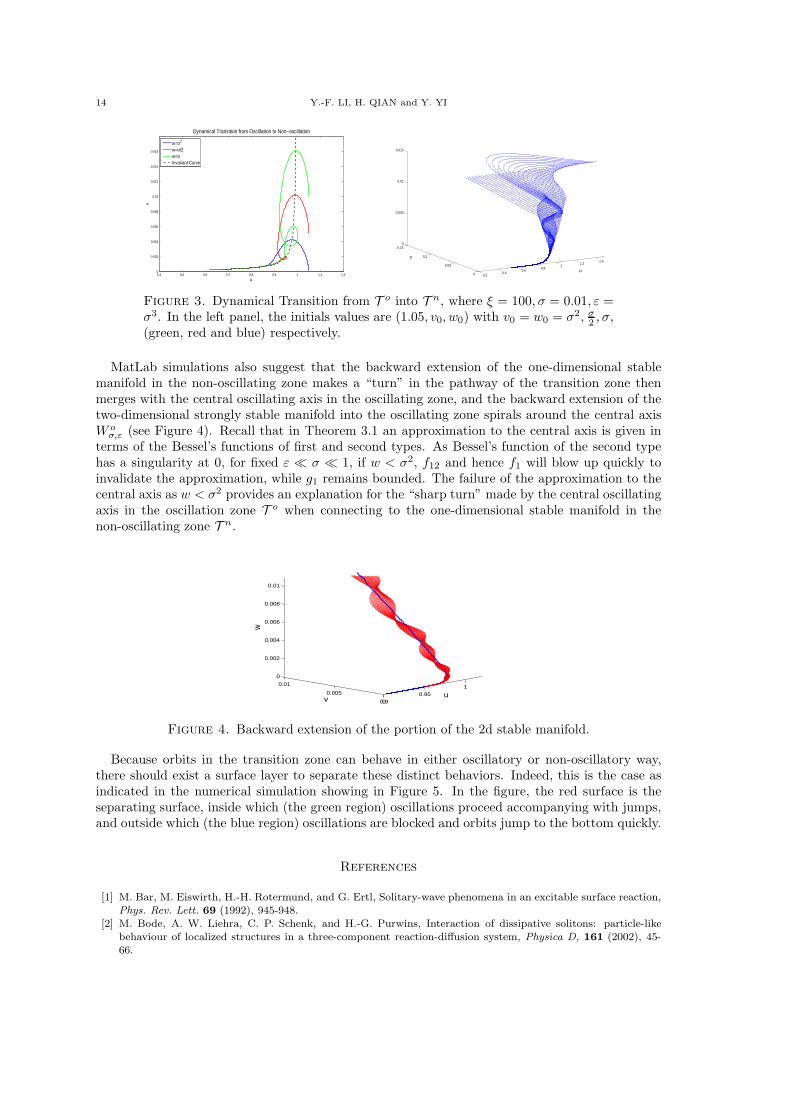
In the left panel of Figure 3, three particular orbits in the transition zone are plotted. Aninteresting phenomenon we observe numerically is that, although an orbit in the oscillating zonehas a decreasing oscillating diameters to the central axis and the diameter is nearly zero at thebottom of the oscillating zone, it can actually reassume some oscillations in the transition zonewith increasing diameters, but as its w value decreases, its number of complete oscillations alsodecreases. Once the orbit exits the transition zone, it immediately follows the two-dimensionalstrong stable manifold in the non-oscillating zone in a monotone fashion.

The right panel of Figure 3 is a MatLab simulation of dynamics in the transition zone. Weobserve that there is a unique, narrow, ‘Tornado”-looking pathway in T t through which the tran-sition occurs. Moreover, no matter where they start in the oscillating zone T o, orbits eventuallycluster in the pathway and then follow the “Tornado tail” to enter the non-oscillating zone T n.We note that for an orbit (u(t), v(t), w(t)) entering in the transition zone, the initial entry valueu0 of u(t) is of the scale �� < 1 < �. It then follows from (1.5) that u(t) ≤ (� − 1)1−�e−�t, that is,u(t) starts to decay exponentially during the transition. This explains the formation of the narrowpathway in the transition zone.


0.4 0.5 0.6 0.7 0.8 0.9 1 1.1 1.20

0.002

0.004

0.006

0.008

0.01

0.012

0.014

0.016

u

v

Dynamical Transition from Oscillation to Non−oscillation

w=σ2

w=σ/2w=σInvariant Curve

0.20.4

0.60.8

11.2

1.4

0

0.05

0.1

0.150

0.005

0.01

0.015

u

v

Figure 3. Dynamical Transition from T o into T n, where � = 100, � = 0.01, " =�3. In the left panel, the initials values are (1.05, v0, w0) with v0 = w0 = �2, �

2 , �,(green, red and blue) respectively.

MatLab simulations also suggest that the backward extension of the one-dimensional stablemanifold in the non-oscillating zone makes a “turn” in the pathway of the transition zone thenmerges with the central oscillating axis in the oscillating zone, and the backward extension of thetwo-dimensional strongly stable manifold into the oscillating zone spirals around the central axisW o

�," (see Figure 4). Recall that in Theorem 3.1 an approximation to the central axis is given interms of the Bessel’s functions of first and second types. As Bessel’s function of the second typehas a singularity at 0, for fixed " ≪ � ≪ 1, if w < �2, f12 and hence f1 will blow up quickly toinvalidate the approximation, while g1 remains bounded. The failure of the approximation to thecentral axis as w < �2 provides an explanation for the “sharp turn” made by the central oscillatingaxis in the oscillation zone T o when connecting to the one-dimensional stable manifold in thenon-oscillating zone T n.

0.90.95

1

0

0.005

0.01

0

0.002

0.004

0.006

0.008

0.01

uv

w

Figure 4. Backward extension of the portion of the 2d stable manifold.

Because orbits in the transition zone can behave in either oscillatory or non-oscillatory way,there should exist a surface layer to separate these distinct behaviors. Indeed, this is the case asindicated in the numerical simulation showing in Figure 5. In the figure, the red surface is theseparating surface, inside which (the green region) oscillations proceed accompanying with jumps,and outside which (the blue region) oscillations are blocked and orbits jump to the bottom quickly.

References

[1] M. Bar, M. Eiswirth, H.-H. Rotermund, and G. Ertl, Solitary-wave phenomena in an excitable surface reaction,Phys. Rev. Lett. 69 (1992), 945-948.

[2] M. Bode, A. W. Liehra, C. P. Schenk, and H.-G. Purwins, Interaction of dissipative solitons: particle-likebehaviour of localized structures in a three-component reaction-diffusion system, Physica D, 161 (2002), 45-66.


12

34

0

0.5

1

1.50

0.002

0.004

0.006

0.008

0.01

0.012

0.014

uv

w

Figure 5. Separation of Oscillation and Non-oscillation in the Transition Zone.

[3] S. R. de Groot and P. Mazur, Nonequilibrium Thermodynamics, (Dover: New York 1984).[4] J. D. Dockery, J. P. Keener and J. J. Tyson, Dispersion of traveling waves in the Belousv-Zhabotinsky

reaction, Physica D, 30 (1988), 177-191.[5] I. R. Epstein and J. A. Pojman, An Introduction to Nonlinear Chemical Dynamics: Oscillation, Waves,

Patterns, and Chaos, Oxford University Press, 1998.[6] N. Fenichel, Geometric singular perturbation for ordinary differental equations, J. Differential Equations 31

(1979), 53-98.[7] R. J. Field and R. M. Noyes, Oscillations in chemical systems. IV. Limit cycle behavior in a model of a real

chemical reaction, J. Chem. Phys. 60 (1974), 1877-1884.[8] C. Grebogi, E. Ott, and J. A. Yorke, Chaotic attractors in crisis, Phys. Rev. Lett. 48 (1982), 1507-1510.[9] C. Grebogi, E. Ott, and J. A. Yorke, Crises, sudden changes in chaotic attractors and chaotic transients,

Physica D 7 (1983), 181-200.[10] J. K. Hale, Dynamical systems and stability, J. Math. Anal. and Appl. 26 (1969), 39–59.[11] S. P. Hastings and J. D. Murray, The existence of oscillatory solucitons in the Field-Noyes model for the

Belousv-Zhabotinsky reaction, SIAM J. Appl. Math. 28 (1975), 678-688.[12] R. D. Janz, D. J. Vanecek and R. J. Field,Composite double oscillation in a modified version of the oregonator

model of the Belousov-Zhabotinsky reaction, J. Chem. Phys. 73 (1980), 3132.[13] D. Q. Jiang, M. Qian, and M. P. Qian, Mathematical Theory of Nonequilibrium Steady States: On the

Frontier of Probability and Dynamical Systems, New York: Springer-Verlag, 2004.[14] J. P. Keener and J. J. Tyson, Spiral waves in the Belousv-Zhabotinsky reaction, Physica D, 21 (1986),

307-324.[15] J. P. Keener and J. J. Tyson, The motion of untwisted untorted scroll waves in the Belousv-Zhabotinsky

reaction, Science, 239 (1988), 1284-1286.[16] K. Kruse and F. Julicher, Oscillations in cell biology, Current Opinion in Cell Biology, 17 (2005), 20-26.[17] J. P. LaSalle, Stability theory for ordinary differential equations, J. Differential Equations, 4 (1968), 57–65.[18] K. J. Lee, W. D. McCormick, J. E. Pearson and H. L. Swinney, Experimental observation of self-replicating

spots in a reaction-diffusion system, Nature, 369 (1994), 215-218.[19] Y.-F. Li, H. Qian, and Y. Yi, Oscillations and multiscale dynamics in a closed chemical reaction system:

Second law of thermodynamics and temporal complexity, J. Chem. Phys. 129, No. 15, (2008), 154505.[20] B. Marts, D. J. W. Simpson, A. Hagberg and A. L. Lin, Period doubling in a periodically forced Belousov-

Zhabotinsky reaction, Phys. Rev. E(3), 76 (2007), 1539-3755.[21] J. D. Murray, Mathematical Biology I: An Introduction, Third ed., Springer, 2002.[22] G. Nicolis and I. Prigogine, Self-organization in Nonequilibrium Systems, Wiley-Interscience, New York,

1977.[23] Y. Nishiura and D. Ueyama, A skeleton structure of self-replicating dynamics, Physica D, 130 (1999), 73-104.[24] R. M. Noyse and R. J. Field, Oscillatory Chemical Reactions, Ann. Rev. Phys. Chem. 25 (1974), 95.[25] H. Qian, Open-system nonequilibrium steady-state: statistical thermodynamics, fluctuations and chemical

oscillations, J. Phys. Chem. B, 110 (2006), 15063-15074.[26] H. Qian, Phosphorylation energy hypothesis: open chemical systems and their biological functions, Ann. Rev.

Phys. Chem. 58 (2007), 113-142.[27] K. Sakamoto, Invariant Manifolds in Singular Perturbation Problems for Ordinary Differential Equations,

Proc. Roy. Soc. Edinburg. A. 116 (1990), 45-78.[28] T. Tel and Y. C. Lai, Chaotic transients in spatially extended systems, Phys. Reports 460 (2008), 245-275.[29] K. Tomita and I. Tsuda, Chaos in the Belousov-Zhabotinsky Reaction in a Flow System, Phys. Lett. A, 71

(1979), 489-492.[30] I. Tsuda, On the abnormality of period doubling bifurcations: in connection with the bifurcation structure in

the Belousov-Zhabotinsky reaction system, Progr. Theoret. Phys. 66 (1981), 1985-2002.


[31] J. J. Tyson, Non-Equilibrium Dynamics in Chemical Systems, (C. Vidal and A. Pacault Eds.), Springer-Verlag,Berlin 1981.

[32] J. Wang, F. Hynne and P. G. Sørensen, Period-doubling geometry of the Belousov-Zhabotinsky reactiondynamics, Int. J. Bifur. Chaos Appl. Sci. Engrg., 6 (1996), 1267-1279.

[33] S. Wiggins and P. Holmes, Periodic orbits in slowly varying oscillators, SIAM J. Math. Anal. 18, No. 3(1987), 592-611.

[34] Y. Yi, Generalized integral manifold theorem, J. Differential Equations 102 No. 1 (1993), 153-187.

Y.-F. Li: Institute for Mathematics and its Applications, University of Minnesota, 207 Church St.

S.E., Minneapolis, MN 55455-0134

E-mail address: [email protected]

H. Qian: Department of Applied Mathematics, University of Washington, Seattle, Washington 98195


Y. Yi: School of Mathematics, Georgia Institute of Technology, Atlanta, Georgia, 30332-0160


nonlinear oscillations and multiscale dynamics …

Documents