nonlinear models of econometric analysisdoubleh/lecturenotes/slides1_summer2012.… · lecture 2:...
TRANSCRIPT

Nonlinear Models of Econometric Analysis
September 2011
1 / 1

Introduction
Linear econometric models are widely popular in economics.
Most people run OLS and 2SLS.
However, there are questions not addressed by OLS or 2SLS.
Linear Models might be misspecified.
Alternatives: nonlinear models, nonparametric models,semiparametric models.
Some nonlinear models can be implemented in Stata: for examplequantile regression, discrete choice models
Some can not, for example auction models, dynamic discrete choicemodels, nonlinear models of demand and oligopolistic competition.
2 / 1
Introduction
Nonlinear Models are challenging, in terms of both numericalimplementation and econometric (statistical analysis).
Econometric analysis focuses more on the statistical properties ofnonlinear models.
But numerical implementation is equally, if not more, difficult!
Some nonlinear models, such quantile regression and discrete choicemodels, can be computed as efficiently as linear models. However,other models are far more difficult.
Ken Judd’s ”Numerical Methods in Economics” is a good startingpoint.
3 / 1

Examples of the difficulty of numerical implementation:
(Knittel)
http://www.nber.org/papers/w14080
(Judd)
http://economics.uchicago.edu/Skrainka-HighPerformanceQuad.pdf
4 / 1

Course Materials
Current course materials are posted at:
http://www.stanford.edu/~doubleh/eco273
http://www.stanford.edu/~doubleh/condensedcourse/
5 / 1

Outline of Materials
Review of General Nonlinear Estimator Theory
Nonparametric Regression, Application to Auctions
Quantile Regression
Simulation, Computation, Markov Chain Monte Carlo (MCMC) andBayesian Methods
Bootstrap and Subsampling
Time permitting: Treatment Effect Models
6 / 1

Lecture 2: Consistency of M-estimators
Instructor: Han Hong
Department of EconomicsStanford University
Prepared by Wenbo Zhou, Renmin University
Han Hong Consistency of M-estimators

References
• Takeshi Amemiya, 1985, Advanced Econometrics, HarvardUniversity Press
• Newey and McFadden, 1994, Chapter 36, Volume 4, TheHandbook of Econometrics.
Han Hong Consistency of M-estimators

Consistency
• Distinction between global and local consistency.
• Global condition: If Θ is compact,
• supθ∈Θ |Qn (θ)− Q (θ) | p−→ 0,
• Q (θ) < Q (θ0) for θ 6= θ0,
then θp−→ θ0, where θ = argmaxθ∈ΘQn (θ)
• Local condition: If N is a neighborhood around θ0,
• supθ∈N
∣∣∣∣∂Qn(θ)∂θ − ∂Q(θ)
∂θ
∣∣∣∣ p−→ 0,
• Q (θ) < Q (θ0) for θ 6= θ0 and θ ∈ N,
then infθ∈Θ ||θ − θ0||p−→ 0, where Θ denotes the set of θ for
which ∂Qn(θ)∂θ = 0.
• For the local consistency condition, check
(1) ∂Q(θ0)∂θ = 0 and (2) ∂2Q(θ0)
∂θ∂θ′ negative definite.
Han Hong Consistency of M-estimators
Consistency for MLE
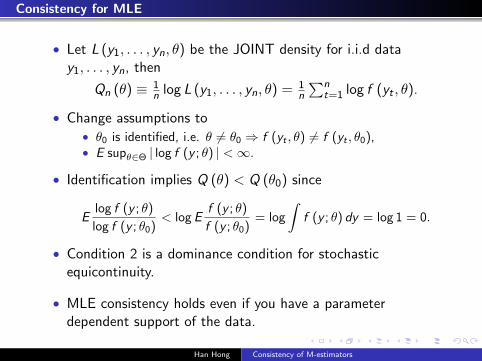
• Let L (y1, . . . , yn, θ) be the JOINT density for i.i.d datay1, . . . , yn, then
Qn (θ) ≡ 1n log L (y1, . . . , yn, θ) = 1
n
∑nt=1 log f (yt , θ).
• Change assumptions to• θ0 is identified, i.e. θ 6= θ0 ⇒ f (yt , θ) 6= f (yt , θ0),• E supθ∈Θ | log f (y ; θ) | <∞.
• Identification implies Q (θ) < Q (θ0) since
Elog f (y ; θ)
log f (y ; θ0)< log E
f (y ; θ)
f (y ; θ0)= log
∫f (y ; θ) dy = log 1 = 0.
• Condition 2 is a dominance condition for stochasticequicontinuity.
• MLE consistency holds even if you have a parameterdependent support of the data.
Han Hong Consistency of M-estimators

• In general case when yt is not i.i.d,
E log L (y1, . . . , yn; θ) ≤ log EL (y1, . . . , yn; θ0)
still holds but to justify the strict < is harder.
• When global condition fails or Θ is not compact, localcondition may hold.
• Example: Mixture of normal distributions.
yt ∼ λN(µ1, σ
21
)+ (1− λ)N
(µ2, σ
22
),
L =n∏
t=1
[λ√
2πσ1
exp
(− (yt − u1)2
2σ21
)+
1− λ√2πσ2
exp
(− (yt − u2)2
2σ22
)].
Set u1 = y1 and let σ1 → 0, then L increases to ∞. Henceglobal MLE cannot be consistent, but local MLE is.
Han Hong Consistency of M-estimators

Consistency for GMM
• Qn (θ) = gn (θ)′Wgn (θ), for gn (θ) = 1n
∑nt=1 g (zt , θ), and
W is the positive definite weighting matrix. If• supθ∈Θ |gn (θ)− Eg (zt , θ) | p−→ 0,
• Eg (zt , θ) = 0 iff θ = θ0,
then θ ≡ argmaxθQn (θ)p−→ 0.
• Global identification in nonlinear GMM model is usuallydifficult and “assumed”.
• But identification in linear models usually reduces to conditionthat the sample var-cov matrix for regressors is full rank, i.e• Extx
′t for iid models,
• limn→∞1n
∑nt=1 xtx
′t for fixed regressors.
• For least square, 1n
∑nt=1 (yt − x ′tβ)2 p−→ E (y − x ′β)2. Iff Extx
′t
full rank,
E (y − x ′β)2 − E (y − x ′β0)
2= E [x ′ (β − β0)]
2
= (β − β0)′ Extx′t (β − β0) > 0 if β 6= β0.
Han Hong Consistency of M-estimators

Quantile Regression
• Conditional τ th quantile of yt given xt is a linear regressionfunction x ′tβ0, i.e. Pr (yt ≤ x ′tβ0|xt) ≡ Fy (x ′tβ0|xt) = τ .
• The τ = 12 th quantile is the median.
• Population moment condition:
E(τ − 1
(yt ≤ x ′tβ0
))xt = E
(τ − Pr
(yt ≤ x ′tβ0|xt
))xt = 0.
• Sample moment condition:
0 ≈1
n
n∑t=1
xt(τ − 1
(yt ≤ x ′t β
))=
1
n
n∑t=1
xt[τ1(y > x ′t β
)− (1− τ) 1
(yt ≤ x ′t β
)].
• Integrate the condition back to obtain the convex objectivefunction Qn (β).
Han Hong Consistency of M-estimators
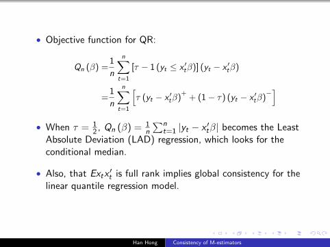
• Objective function for QR:
Qn (β) =1
n
n∑t=1
[τ − 1 (yt ≤ x ′tβ)] (yt − x ′tβ)
=1
n
n∑t=1
[τ (yt − x ′tβ)
++ (1− τ) (yt − x ′tβ)
−]
• When τ = 12 , Qn (β) = 1
n
∑nt=1 |yt − x ′tβ| becomes the Least
Absolute Deviation (LAD) regression, which looks for theconditional median.
• Also, that Extx′t is full rank implies global consistency for the
linear quantile regression model.
Han Hong Consistency of M-estimators
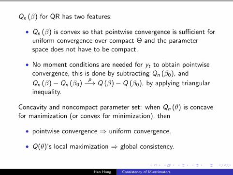
Qn (β) for QR has two features:
• Qn (β) is convex so that pointwise convergence is sufficient foruniform convergence over compact Θ and the parameterspace does not have to be compact.
• No moment conditions are needed for yt to obtain pointwiseconvergence, this is done by subtracting Qn (β0), and
Qn (β)− Qn (β0)p−→ Q (β)− Q (β0), by applying triangular
inequality.
Concavity and noncompact parameter set: when Qn (θ) is concavefor maximization (or convex for minimization), then
• pointwise convergence ⇒ uniform convergence.
• Q(θ)’s local maximization ⇒ global consistency.
Han Hong Consistency of M-estimators

Uniform Convergence (in probability)
• Definition: Q (θ) converges in probability to Q (θ) uniformlyover the compact set θ ∈ Θ if
∀ε > 0, limT→∞
P
(supθ∈Θ|Q (θ)− Q (θ) | > ε
)= 0.
• Consistency of M-Estimators: If
• QT (θ) converges in probability to Q (θ) uniformly,
• Q (θ) continuous and uniquely maximized at θ0,
• θ = argmaxQT (θ) over compact parameter set Θ,
plus continuity and measurability for QT (θ), then θp−→ θ0.
• Consistency of estimated var-cov matrix: Note that it issufficient for uniform convergence to hold over a shrinkingneighborhood of θ0.
Han Hong Consistency of M-estimators

Conditions for Uniform Convergence: Equicontinuity
First think about sequence of deterministic functions fn (θ).
• Uniform Equicontinuity for fn (θ):
limδ→0
supn
sup|θ′−θ|<δ
|fn(θ′)− fn (θ) | = 0.
• What if fn (θ) may be discontinuous but the size of the jumpgoes to 0?
• Asymptotic uniform equicontinuity for fn (θ):
limδ→0
lim supn→∞
sup|θ′−θ|<δ
|fn(θ′)− fn (θ) | = 0.
• Uniform convergence of fn (θ):Θ compact, supθ∈Θ |fn (θ) | −→ 0 if and only if fn (θ) −→ 0for each θ and fn is asymptotically uniformly equicontinuous.
Han Hong Consistency of M-estimators

Then the stochastic case Qn (θ).
• Definition:
A sequence of random functions Qn (θ) is stochastic uniformequicontinuity if ∀ε > 0,
limδ→0
lim supn→∞
P
(sup
|θ−θ′|<δ|Qn (θ)− Qn (θ′) | > ε
)= 0.
• Uniform convergence in probability:
If Qn (θ)p−→ 0 for each θ, and Qn (θ) is stochastic
equicontinuous on θ ∈ Θ compact, then
supθ∈Θ|Qn (θ) | p−→ 0.
Han Hong Consistency of M-estimators

Lipschitz Condition for Stochastic Equicontinuity
• Simple sufficient condition for stochastic equicontinuity.• where the objective function is smooth, differentiable, etc.
• Lipschitz condition: For ∀θ, θ′ ∈ Θ, if
|Qn (θ)− Qn (θ′) | ≤ Bnd (θ, θ′),
where limδ→0 sup|θ−θ′|<δ d (θ, θ′) = 0 and Bn = Op (1),then Qn (θ) is stochastic equicontinuous.
• Example: Suppose Qn (θ) = 1n
∑nt=1 f (zt , θ), zt iid, f (zt , θ)
differentiable with fθ (zt , θ), then by Taylor, for θ ∈ (θ, θ′),
|Qn (θ)− Qn (θ′) | ≤ 1
n
n∑t=1
|fθ(zt , θ
)||θ − θ′|.
If b (zt) = supθ∈Θ fθ (zt , θ) is such that Eb (zt) <∞, thenthe Lipschitz condition holds with Bn = 1
n
∑nt=1 b (zt).
Han Hong Consistency of M-estimators

Uniform WLLN
• But what to do when the Lipschitz condition is notapplicable?
• Uniform WLLN
Θ compact, yt iid, g (yt , θ) continuous in θ for each yt a.s.,Eg (yt , θ) = 0, E supθ∈Θ |g (yt , θ) | <∞, then ∀ε > 0,
limn→∞
P
(supθ∈Θ|1n
n∑t=1
g (yt , θ) | > ε
)= 0.
Han Hong Consistency of M-estimators

Proof: Use pointwise convergence + stochastic equicontinuity.
1 E supθ∈Θ |g (yt , θ) | <∞ =⇒ E |g (yt , θ) | >∞ for each θ, so
use SLLN 2 to conclude 1n
∑nt=1 g (yt , θ)
a.s.(p)−→ 0 for each θ.
2 Verify stochastic equicontinuity for 1n
∑nt=1 g (yt , θ):
sup|θ−θ′|<δ
|1n
n∑t=1
g (yt , θ)− g(yt , θ
′) |≤ sup|θ−θ′|<δ
1
n
n∑t=1
|g (yt , θ)− g(yt , θ
′) |≤ 1
n
n∑t=1
sup|θ−θ′|<δ
|g (yt , θ)− g(yt , θ
′) |.
Han Hong Consistency of M-estimators

Therefore
limδ→0
lim supn→∞
P
(sup
|θ−θ′|<δ|1n
n∑t=1
g (yt , θ)− g(yt , θ
′) | > ε
)
≤ limδ→0
lim supn→∞
P
(1
n
n∑t=1
sup|θ−θ′|<δ
|g (yt , θ)− g(yt , θ
′) | > ε
)
≤ limδ→0
lim supn→∞
E∑n
t=1 sup|θ−θ′|<δ |g (yt , θ)− g (yt , θ′) |
nε
= limδ→0
E sup|θ−θ′|<δ
|g (yt , θ)− g(yt , θ
′) |Finally use (uniform b/o compact Θ) continuity of g (yt , θ) and
DOM. Since limδ→0 sup|θ−θ′|<δ |g (yt , θ)− g (yt , θ′) | almost surely,
andE supδ sup|θ−θ′|<δ |g (yt , θ)− g (yt , θ
′) | < E2 supθ |g (yt , θ) | <∞.
Han Hong Consistency of M-estimators

Lecture 3: Asymptotic Normality of M-estimators
Instructor: Han Hong
Department of EconomicsStanford University
Prepared by Wenbo Zhou, Renmin University
Han Hong Normality of M-estimators

References
• Takeshi Amemiya, 1985, Advanced Econometrics, HarvardUniversity Press
• Newey and McFadden, 1994, Chapter 36, Volume 4, TheHandbook of Econometrics.
Han Hong Normality of M-estimators

Asymptotic Normality
The General Framework
• Everything is just some form of first order Taylor Expansion:
∂Qn(θ)
∂θ= 0⇐⇒
√n∂Qn (θ0)
∂θ+√n(θ − θ0
) ∂2Qn (θ∗)
∂θ∂θ′= 0.
√n(θ − θ0
)=−
(∂2Qn (θ∗)
∂θ∂θ′
)−1√n∂Qn (θ0)
∂θ
LD= −
(∂2Q (θ0)
∂θ∂θ′
)−1√n∂Qn (θ0)
∂θ
d−→ N(0,A−1BA−1
)where
A = E
(∂2Q (θ0)
∂θ∂θ′
), B = Var
(√n∂Qn (θ0)
∂θ
)
Han Hong Normality of M-estimators
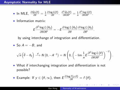
Asymptotic Normality for MLE
• In MLE, ∂Qn(θ)∂θ = 1
n∂ log L(θ)
∂θ . ∂2Qn(θ)∂θ∂θ′ = 1
n∂2 log L(θ)∂θ∂θ′ .
• Information matrix:
E∂2 log L (θ0)
∂θ∂θ′= −E ∂ log L (θ0)
∂θ
∂ log L (θ0)
∂θ′.
by using interchange of integration and differentiation.
• So A = −B, and
√n(θ − θ0
)d−→ N
(0,−A−1
)= N
(0,
(− lim
1
nE∂2 log L (θ)
∂θ∂θ′
)−1).
• What if interchanging integration and differentiation is notpossible?
• Example: If y ∈ (θ,∞), then E ∂ log f (y ;θ)∂θ = f (θ).
Han Hong Normality of M-estimators
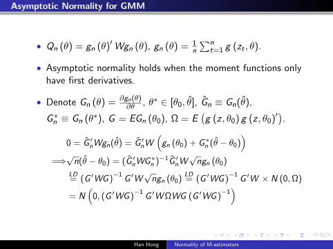
Asymptotic Normality for GMM
• Qn (θ) = gn (θ)′Wgn (θ), gn (θ) = 1n
∑nt=1 g (zt , θ).
• Asymptotic normality holds when the moment functions onlyhave first derivatives.
• Denote Gn (θ) = ∂gn(θ)∂θ , θ∗ ∈ [θ0, θ], Gn ≡ Gn(θ),
G ∗n ≡ Gn (θ∗), G = EGn (θ0), Ω = E(g (z , θ0) g (z , θ0)′
).
0 = G ′nWgn(θ) = G ′nW(gn (θ0) + G∗n (θ − θ0)
)=⇒√n(θ − θ0) = (G ′nWG∗n )−1G ′nW
√ngn (θ0)
LD= (G ′WG )
−1G ′W
√ngn (θ0)
LD= (G ′WG )
−1G ′W × N (0,Ω)
= N(
0, (G ′WG )−1
G ′WΩWG (G ′WG )−1)
Han Hong Normality of M-estimators
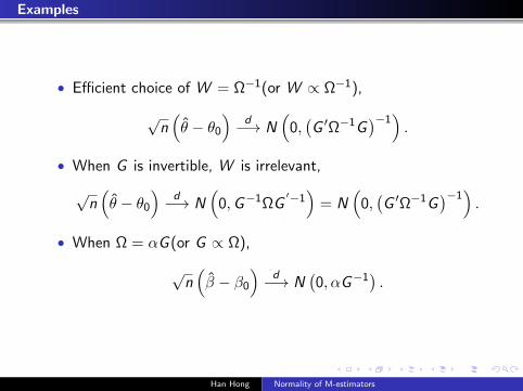
Examples
• Efficient choice of W = Ω−1(or W ∝ Ω−1),
√n(θ − θ0
)d−→ N
(0,(G ′Ω−1G
)−1).
• When G is invertible, W is irrelevant,
√n(θ − θ0
)d−→ N
(0,G−1ΩG
′−1)
= N(
0,(G ′Ω−1G
)−1).
• When Ω = αG (or G ∝ Ω),
√n(β − β0
)d−→ N
(0, αG−1
).
Han Hong Normality of M-estimators

• Least square (LS): g (z , β) = x (y − xβ).
• G = Exx ′, Ω = Eε2xx ′, then
√n(β − β0
)d−→ N
(0, (Exx ′)
−1 (Eε2xx ′
)(Exx ′)
−1),
the so-called White’s heteroscedasticity consistency standarderror.
• If E[ε2|x
]= σ2, then Ω = σ2G and
√n(β − β0
)d−→ N
(0, σ2 (Exx ′)
−1).
• Weighted LS: g (z , β) = 1E(ε2|x) (y − x ′β).
G = E 1E(ε2|x)xx
′ = Ω =⇒√n(β − β0
)d−→ N (0,G ).
Han Hong Normality of M-estimators

• Linear 2SLS: g (z , β) = z (y − xβ).
• G = Ezx ′, Ω = Eε2zz ′, W = (Ezz ′)−1, then√n(β − β0
)d−→ N (0,V ).
• If Eε2zz ′ = σ2Ezz ′, V = σ2[Exz ′ (Ezz ′)
−1Ezx ′
]−1.
• Linear 3SLS: g (z , β) = z (y − xβ).
G = Ezx ′, Ω = Eε2zz ′, W =(Eε2zz ′
)−1, then
√n(β − β0
)d−→ N (0,V ) for V =
[Exz ′
(Eε2zz ′
)−1Ezx ′
]−1.
• MLE as GMM: g (z , θ) = ∂ log f (z,θ)∂θ .
G = −E ∂2 log f (z,θ)∂θ∂θ′ = Ω = E ∂ log f (z,θ)
∂θ∂ log f (z,θ)
∂θ′ , then
√n(θ − θ
)d−→ N
(0,G−1
)= N (0,Ω).
Han Hong Normality of M-estimators

• GMM again:
• Take linear combinations of the moment conditions to make
Number of g (z , θ) = Number of θ.
• In particular, take h (z , θ) = G ′Wg (z , θ) and use h (z , θ) asthe new moment conditions, then
θ = argmaxθ
[1
n
n∑t=1
h (zt , θ)
]′ [1
n
n∑t=1
h (zt , θ)
]
is asymptotically equivalent to θ = argmaxθg′nWgn, where
G = E ∂h(z,θ)∂θ = G ′WG , Ω = Eh (z , θ) h (z , θ)′ = G ′WΩWG .
Han Hong Normality of M-estimators

• Quantile Regression as GMM:
• g (z , β) = (τ − 1 (y ≤ x ′β)) x , and W is irrelevant.
• G = E g(z,β)∂β = −E ∂1(y≤x′β)x
∂β . Proceeding with a “quick anddirty” way – take expectation before taking differentiation:
G =∂E1 (y ≤ x ′β) x
∂β=∂ExF (y ≤ x ′β|x)
∂β
=Ex∂F (y ≤ x ′β|x)
∂β= Efy (x ′β|x) xx ′ = Efu (0|x) xx ′.
• Conditional on x , τ − 1 (y ≤ x ′β0) = τ − 1 (u ≤ 0) is a
Bernoulli r.v.⇒ E[(τ − 1 (y ≤ x ′β0))2 |x
]= τ (1− τ), then
Ω = EE[(τ − 1 (y ≤ x ′β0))
2 |x]xx ′ = τ (1− τ)Exx ′.
Han Hong Normality of M-estimators

• Quantile Regression as GMM:
•√n(β − β0)
d→N(
0, τ (1− τ) [Efu (0|x) xx ′]−1
Exx ′ [Efu (0|x) xx ′]−1)
.
• f (0|x) = f (0) if homoscedastic, then V = τ(1−τ)f (0) Exx ′.
• Consistent estimation of G and Ω:
• Estimated by G.
= 1n
∑nt=1
∂g(zt ,θ)∂θ .
• For nonsmooth problems as quantile regression, useQn(θ+2hn)+Qn(θ−2hn)−2Q(θ)
4h2nto approximate.
Require hn = o (1) and 1/hn = o(1/√n).
• For stationary data, heteroscedasticity and dependence willonly affect estimation of Ω. For independent data, use White’sheteroscedasticity-consistent estimate; for dependent data, useNewey-West’s autocorrelation-consistent estimate.
Han Hong Normality of M-estimators

Iteration and One Step Estimation
• The initial guess θ ⇒ the next round guess θ.
• Newton-Raphson, use quadratic approximation for Qn (θ).
• Gauss-Newton, use linear approximation for the first-ordercondition, e.g. GMM.
• If the initial guess is a√n consistent estimate, more iteration
will not increase (first-order) asymptotic efficiency.
• e.g.(θ − θ0
)= Op
(1√n
), then
√n(θ − θ0
) LD=√n(θ − θ0
),
for θ = argmaxθQn (θ).
Han Hong Normality of M-estimators

Influence Function
• φ (zt) is called influence function if
•√n(θ − θ0) = 1√
n
∑nt=1 φ (zt) + op (1),
• Eφ (zt) = 0, Eφ (zt)φ (zt)′<∞.
• Think of√n(θ − θ0) distributed as
φ (zt) ∼ N(0,Eφφ′
).
• Used for discussion of asymptotic efficiency, two step ormultistep estimation, etc.
Han Hong Normality of M-estimators

Examples
• For MLE,
φ (zt) =
[−E ∂
2 ln f (yt , θ0)
∂θ∂θ′
]−1∂ ln f (yt , θ0)
∂θ
=
[E∂ ln f (yt , θ0)
∂θ
∂ ln f (yt , θ0)
∂θ′
]−1 ∂ ln f (yt , θ0)
∂θ.
• For GMM,
φ =−(G ′WG
)−1G ′Wg (zt , θ0) ,
or φ =−(E∂h
∂θ
)−1h (zt , θ0) for h (zt , θ0) = G ′Wg (zt , θ0) .
• Quantile Regression:
φ (zt) =[Ef (0|x) xx ′
]−1(τ − 1 (u ≤ 0)) xt .
Han Hong Normality of M-estimators

Asymptotic Efficiency
• Is MLE efficient among all asymptotically normal estimators?
• Superefficient estimator:
Suppose√n(θ − θ0)
d−→ N (0,V ) for all θ. Now define
θ∗ =
θ if |θ| ≥ n−1/4
0 if |θ| < n−1/4
then√n (θ∗ − θ0)
d−→ N (0, 0) if θ0 = 0, and√n (θ∗ − θ0)
LD=√n(θ − θ0)
d−→ N (0,V ) if θ0 6= 0.
• θ is regular if for any data generated by θn = θ0 + δ/√n, for
δ ≥ 0,√n(θ − θ0) has a limit distribution that does not
depend on δ.
Han Hong Normality of M-estimators

• For regular estimators, influence function representationindexed by τ ,
√n(θ (τ)− θ0)
LD= φ (z , τ) ∼ N
(0,Eφ (τ)φ (τ)′
),
• θ (τ) is efficient than θ (τ) if it has a smaller var-cov matrix.
• A necessary condition is thatCov (φ (z , τ)− φ (z , τ) , φ (z , τ)) = 0 for all τ including τ .
• The following are equivalent:
Cov (φ (z , τ)− φ (z , τ) , φ (z , τ)) = 0
⇐⇒Cov (φ (z , τ) , φ (z , τ)) = Var (φ (z , τ))
⇐⇒Eφ (z , τ)φ (z , τ)′ = Eφ (z , τ)φ (z , τ)′
Han Hong Normality of M-estimators

Newey’s efficiency framework:
• Classify estimators into the GMM framework with
φ (z , τ) = D (τ)−1m (z , τ).
• For the class indexed by τ = W , given a vector g (z , θ0),
D (τ) ≡ D (W ) = G ′WG and
m (z , τ) ≡ m (z ,W ) = G ′Wg (z , θ0).
• Consider MLE among the class of GMM estimators, so that τindexes any vector of moment function having the samedimension as θ. In this case,
D (τ) ≡ D (h) = −E ∂h∂θ and m (z , τ) = h (zt , θ0).
Han Hong Normality of M-estimators

• For this particular case where φ (z , τ) = D (τ)−1m (z , τ),
Eφ (z , τ)φ (z , τ)′ = Eφ (z , τ)φ (z , τ)′ =⇒
D (τ)−1 Em (z , τ)m (z , τ)D (τ)−1 = D (τ)−1 Em (z , τ)m (z , τ)D (τ)−1 .
• If τ satisfies D (τ) = Em (z , τ)m (z , τ) for all τ , then bothsides above are the same D (τ)−1 and so efficient.
• Examples. Check D (τ) = Em (z , τ)m (z , τ).
• GMM with optimal weighting matrix:
D (τ) = G ′WG , m (z , τ) = m (z ,W ) = G ′Wg(z , θ0).
To check D (τ) = Em (z , τ)m (z , τ) = G ′WΩWG ,
G ′WG = G ′WΩWG =⇒ ΩW = I =⇒ W = Ω−1.
Han Hong Normality of M-estimators
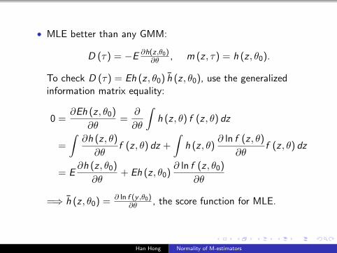
• MLE better than any GMM:
D (τ) = −E ∂h(z,θ0)∂θ , m (z , τ) = h (z , θ0).
To check D (τ) = Eh (z , θ0) h (z , θ0), use the generalizedinformation matrix equality:
0 =∂Eh (z , θ0)
∂θ=
∂
∂θ
∫h (z , θ) f (z , θ) dz
=
∫∂h (z , θ)
∂θf (z , θ) dz +
∫h (z , θ)
∂ ln f (z , θ)
∂θf (z , θ) dz
= E∂h (z , θ0)
∂θ+ Eh (z , θ0)
∂ ln f (z , θ0)
∂θ
=⇒ h (z , θ0) = ∂ ln f (y ,θ0)∂θ , the score function for MLE.
Han Hong Normality of M-estimators

Two Step Estimator
General Framework:
• First step estimator√n (γ − γ0) = 1√
n
∑nt=1 φ (zt) + op (1).
• Estimate θ by
∂Qn(θ, γ)
∂θ=
1
n
n∑t=1
q(zt , θ, γ)
∂θ= 0
Let=
1
n
n∑t=1
h(zt , θ, γ).
• Let
H (z , θ, γ) =∂h (z , θ, γ)
∂θ, Γ (z , θ, γ) =
∂h (z , θ, γ)
∂γ;
H = EH (zt , θ0, γ0) , Γ = EΓ (z , θ0, γ0) ;
h = h (θ0, γ0) .
Han Hong Normality of M-estimators

• Then just taylor expand: 1√n
∑h(zt , θ, γ
)= 0
⇐⇒ 1√n
∑h (θ0, γ) + 1
n
∑H (θ∗, γ)
√n(θ − θ0
)= 0 =⇒
√n(θ − θ0
)=−
[1
n
∑H (θ∗, γ)
]−11√n
∑h (θ0, γ)
LD= − H−1
[1√n
∑h (θ0, γ0) +
1
n
∑Γ (θ0, γ
∗)√n (γ − γ0)
]LD= − H−1
[1√n
∑h + Γ
(1√n
∑φ (zt) + op (1)
)]LD= − H−1
[1√n
∑h + Γ
1√n
∑φ (zt)
].
So that√n(θ − θ0
)d−→ N (0,V ) for
V = H−1E (h + Γφ) (h′ + φ′Γ′)H−1′.
Han Hong Normality of M-estimators
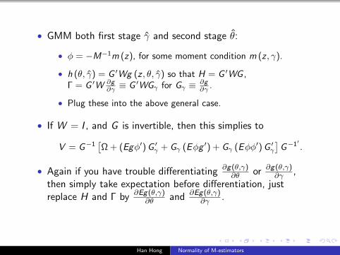
• GMM both first stage γ and second stage θ:
• φ = −M−1m (z), for some moment condition m (z , γ).
• h (θ, γ) = G ′Wg (z , θ, γ) so that H = G ′WG ,Γ = G ′W ∂g
∂γ ≡ G ′WGγ for Gγ ≡ ∂g∂γ .
• Plug these into the above general case.
• If W = I , and G is invertible, then this simplies to
V = G−1[Ω + (Egφ′)G ′γ + Gγ (Eφg ′) + Gγ (Eφφ′)G ′γ
]G−1
′.
• Again if you have trouble differentiating ∂g(θ,γ)∂θ or ∂g(θ,γ)
∂γ ,then simply take expectation before differentiation, justreplace H and Γ by ∂Eg(θ,γ)
∂θ and ∂Eg(θ,γ)∂γ .
Han Hong Normality of M-estimators
Lecture 4: Basic Nonparametric Estimation
Instructor: Han Hong
Department of EconomicsStanford University
2011
Han Hong Basic Nonparametric Estimation

Basic View
• There can be many meanings to “nonparametrics”.
• One meaning is optimization over a set of function.
• For example, given the sample of observations x1, . . . , xn, finda distribution function under which the joint probability ofx1, . . . , xn is maximized.
• This is also called “nonparametric maximum likelihood”.
• The meaning of “nonparametric” for now is density estimateand estimation of conditional expectations.
Han Hong Basic Nonparametric Estimation

Density Estimate: Motivation
• One motivation is to first use the histogram to estimate thedensity:
1
2h
# of xi in (x − h, x + h)
n=
1
2h
1
n
n∑t=1
1 (x − h ≤ xi ≤ x + h)
=1
nh
n∑i=1
1
21
(|x − xi |
h≤ 1
)• 1
21 (|x | ≤ 1) is the uniform density over (−1, 1), called theuniform kernel.
• Generally, use other density function K (·) to get
f (x) =1
nh
n∑t=1
K
(x − xi
h
).
Han Hong Basic Nonparametric Estimation

• Another motivation is to estimate the distribution functionF (x) by
F (x) =1
n
n∑t=1
1 (xi ≤ x) ,
but you can’t differentiate it to get the density.
• Replace 1 (xi ≤ x) by G(xi−xh
)where G (·) is any smooth
distribution function (G (∞) = 1,G (−∞) = 0), and h→ 0.
• In practice, take h as some small but fixed number, like 0.1.
• So let K = G ′ (·), differentiate F (x) to get
f (x) =1
nh
n∑t=1
K
(xi − x
h
)or
1
nhd
n∑t=1
K
(xi − x
h
)if x ∈ Rd .
Han Hong Basic Nonparametric Estimation

Conditional Expectation: Motivation
• Estimate E (y |x) or more generally E (g (y) |x) for somefunction g (·), or things like conditional quantiles.
• Local weighting: use observations xi close to x .
• Take a neighborhood N around x and the size of N shouldshrink to 0 but not too fast.
• Average over those yi for which xi ∈ N .
• More generally give more weights to those yi if xi is close to x ,and less weights to those yi if xi is far away from x .
• For weights Wn (x , xi ) such that
(1)∑n
i=1Wn (x , xi ) = 1, (2) Wn (x , xi )→ 0 if xi 6= x ,
(3) max1≤i≤n |Wn (x , xi ) | → 0 as n→∞,
estimate E (y |x) by∑n
i=1Wn (x , xi )Yi .
Han Hong Basic Nonparametric Estimation

Classification
• Anything you do parametrically, if you do that only for xiclose to x , then you become “nonparametric”.
• Local nonparametric estimates:
• kernel smoothing
• k-nearest neighborhood (k-NN)
• local polynomials
• Global nonparametric estimates:
• series (sieve)
• splines
• The focus today is kernel.
Han Hong Basic Nonparametric Estimation
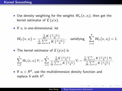
Kernel Smoothing
• Use density weighting for the weights Wn (x , xi ), then get thekernel estimator of E (y |x).
• If xi is one-dimensional, let
Wn (x , xi ) =1nhK
(x−xih
)1nh
∑ni=1 K
(x−xih
) , satisfyingn∑
i=1
Wn (x , xi ) = 1.
• The kernel estimator of E (y |x) is
n∑i=1
Wn (x , xi )Yi =n∑
i=1
1nhK
(x−xih
)1nh
∑ni=1 K
(x−xih
)Yi =1nh
∑ni=1 K
(x−xih
)Yi
1nh
∑ni=1 K
(x−xih
) .
• If xi ∈ Rd , use the multidimension density function andreplace h with hd .
Han Hong Basic Nonparametric Estimation

Another View of Kernel Estimator
• Estimate γ (x) and f (x) separately for
E (y |x) =E (y |x) f (x)
f (x)=
∫yf (y , x) dy
f (x)=γ (x)
f (x)
• f (x) = 1nhd
∑ni=1 K
(x−xih
).
• For γ (x), plug
f (x , y) =1
nhd+1
n∑i=1
K
(x − xih
)K
(yi − y
h
)into
∫yf (y , x) dy , and let u = (yi − y) /h:∫
y f (y , x) dy =1
nhd
n∑i=1
K
(x − xih
)∫y
1
hK
(yi − y
h
)dy
=1
nhd
n∑i=1
K
(x − xih
)∫(yi + uh) K (u) du =
1
nhd
n∑i=1
K
(x − xih
)yi .
Han Hong Basic Nonparametric Estimation

• Another view for γ (x): think of∫y f (y , x) dy as
∫ydP,
where P is the measure over y defined by
P (yi ≤ y , xi = x) =d
dxP (yi ≤ y , xi ≤ x)
estimate=
d
dx
1
n
n∑i=1
1 (yi ≤ y)G
(xi − x
h
)=
1
nhd
n∑i=1
1 (yi ≤ y)K
(xi − x
h
)• Plug in this estimate of P into
∫ydP:∫
ydP =
∫yd
1
nhd
n∑i=1
1 (yi ≤ y)K
(xi − x
h
)
=1
nhd
n∑i=1
K
(xi − x
h
)∫yd1 (yi ≤ y) =
1
nhd
n∑i=1
K
(xi − x
h
)yi
Han Hong Basic Nonparametric Estimation
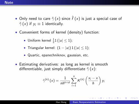
Note
• Only need to care γ (x) since f (x) is just a special case ofγ (x) if yi ≡ 1 identically.
• Convenient forms of kernel (density) function:
• Uniform kernel 121 (|u| ≤ 1);
• Triangular kernel: (1− |u|) 1 (|u| ≤ 1);
• Quartic, epanechniknov, gaussian, etc.
• Estimating derivatives: as long as kernel is smoothdifferentiable, just simply differentiate γ (x):
γ(k) (x) =1
nhk+d
n∑i=1
K (k)
(xi − x
h
)yi
Han Hong Basic Nonparametric Estimation

k-NN and Local Polynomials
• Other two major weighting schemes for Wni (x).
• k-nearest neighborhood (k-NN)
• Use k closest neighbors of point x instead of fixed one.
• Weight these k neighbors equally or according to distances.
• Example: use any kernel density weight K (·).
• Local polynomial
• Run a kth polynomial regression using observations over|xi − x | ≤ h.
• The degree k corresponds to the order of the kernel.
Han Hong Basic Nonparametric Estimation

Series and Splines
• Series (Sieve)
• The only difference between series and local polynomials isthat you run the polynomials using all observations, instead ofonly a shrinking neighborhood (x − h, x + h).
• Instead of fixing k , let k →∞.
• Instead of using polynomials, use family of orthogonal series offunctions, like trigonometric function, etc.
• Splines
• Find a twice differentiable function g (x) that minimizes∑ni=1 (yi − g (xi ))2 + λ
∫g ′′ (x)2 dx , for some λ > 0.
• λ∫g ′′ (x)2 dx is to penalize the roughness of the estimate g .
• This will give a cubic polynomial with continuous secondderivatives.
Han Hong Basic Nonparametric Estimation

Optimal Rate of Convergence for Nonparametric Estimates
• Curse of dimensionality:For a given bandwidth (window size), the higher dimension x ,the less data in a neighborhood with bandwidth h.
• If both h→ 0 and nhd →∞, then the estimate is consistent.
• How about the speed at which estimator converges?
• Conclusion:Suppose the true function γ (x) is pth degree differentiable,all pth derivative bounded uniformly over x . Then the optimal
bandwidth hopt is n−1
2p+d , and the best rate at which γ (x)
can approach γ (x) is Op
(n−
p2p+d
).
Han Hong Basic Nonparametric Estimation

• The problem here is the bias and variance trade-off.• The smaller the h, the smaller the bias, but the less
observations you have, thus the large the variance.
• Criterion: total error = bias + estimation error , or MSE .
• The bias is Op(hp).
• Use p bounded derivatives condition and taylor expansion.
• The variation is Op
(1√nhd
).
• Think of x − µ = Op
(1√n
), by analogy with nhd .
• Total error is Op
(hp + 1√
nhd
).
Han Hong Basic Nonparametric Estimation

• Find a h to minimize total error,
hopt = O(n−
12p+d
).
• Then the (pointwise) optimal rate of convergence is
O(hpopt
)= O
(1√nhd
)= O
(n−
p2p+d
).
• It is not possible to have√n convergence for nonparametric
estimates since p2p+d <
12 .
• Sometimes n1/4 rate of convergence is needed for getting ridof the second order terms for semiparametric estimators,which means p > d/2.
Han Hong Basic Nonparametric Estimation

Optimal Rate for Derivative Estimates
• The optimal bandwidth of γ(k) (x) is of the same order asthat of estimating γ (x) itself.
• The bias is Op(hp−k), and the variation is Op
(1
hk√nhd
).
• The total error is Op
(hp−k + 1
hk√nhd
).
• Find a h to minimize this again,
hopt = n−1
2p+d .
• Then the best convergence rate is
Op
(np−k
)= Op
(1
hk√nhd
)= Op
(n−
p−k2p+d
).
Han Hong Basic Nonparametric Estimation

Higher Order Kernels
• A kernel of order r is defined as those K (·) for which:∫K (u) du = 1,
∫K (u) uqdu = 0,∀q = 1, . . . , r − 1,∫
|urK (u) |du <∞.
• Bias of kernel estimates = E γ (x)− γ (x)
E γ (x) =E1
nhd
n∑i=1
K
(x − xih
)Yi =
∫1
hdK
(x − xih
)E (yi |xi ) f (xi ) dxi
=
∫1
hdK
(x − xih
)γ (xi ) dxi =
∫K (u) γ (x + uh) du
=γ (x) +r−1∑j=1
hjγ(j)
j!
∫ujk (u) du + hr
1
r !
∫γ(r) (x∗) urK (u) du
• If γ (x) has pth bounded derivatives and the kernel is of orderr , then the bias = hmin(p,r).
Han Hong Basic Nonparametric Estimation

• Variance of kernel estimates:
Var (γ(x)) =1
n2h2d
n∑i=1
Var
(K
(x − xih
)Yi
)
=1
nh2dE
(K 2
(x − xih
)Y 2i
)− 1
nh2d
(EK
(x − xih
)Yi
)2
=1
nhd
∫1
hdK 2
(x − xih
)E(y2i |xi)f (xi ) dxi −
1
n
(E
1
hdK
(x − xih
)Yi
)2
=1
nhd
∫1
hdK 2
(x − xih
)g (xi ) dxi + O
(1
n
)=
1
nhd
∫K 2 (u) g (x + uh) du + O
(1
n
)=
1
nhd
∫K 2 (u) g (x) du +
1
nhdh
∫K 2 (u) g ′ (x∗) udu + O
(1
n
)=
1
nhd
∫K 2 (u) g (x) du + O
(1
nhdh
)+ O
(1
n
)= O
(1
nhd
)
Han Hong Basic Nonparametric Estimation

Asymptotic Distribution, Confidence Band
• If use h ∼ hopt , the asymptotic distribution will depend onboth the bias and the variance.
• If use h << hopt , i.e., hhopt→ 0, the asymptotic distribution
has no bias in but the convergence rate is not the fastest.
• Example: consider d = 1, r = 2, then hopt = n−1
2p+d = n−15 .
• Find the asymptotic distribution of√nhopt (m (x)−m (x)) = h−2opt (m (x)−m (x)) ,
for m (x) = γ(x)
f (x).
Han Hong Basic Nonparametric Estimation

Bias
• Linearization
m (x)−m (x) ≈ 1
f (x)(γ (x)− γ (x))− γ (x)
f (x)2
(f (x)− f (x)
)• As seen above, E γ (x)− γ (x) = 1
2h2γ′′ (x)
∫u2K (u) du.
• E f (x)− f (x) = 12h
2f ′′ (x)∫u2K (u) du,
since γ (x) = m (x) f (x) and m (x) ≡ 1.
• Therefore,
Eh−2opt (m (x)−m (x)) =1
2
(γ′′
f− m
ff ′′)∫
u2K (u) du
=1
2
(m′′f + 2m′f ′ + mf ′′
f− m
ff ′′)∫
u2K (u) du
=1
2
2m′ (x) f ′ (x) + m′′ (x) f (x)
f (x)
∫u2K (u) du.
Han Hong Basic Nonparametric Estimation

Variance
• As seen above, for g (x) = E(y2|x
)f (x),
Var(√
nh (γ (x)− γ (x)))→ g (x)
∫K 2 (u) du.
• Var(√
nh(f (x)− f (x)))→ f (x)
∫K 2 (u) du since for density
estimate where y ≡ 1, g (x) = f (x).
• The covariance between γ (x) and f (x):
Cov(√
nh (γ (x)− γ (x)) ,√nh(f (x)− f (x))
)→ γ (x)
∫K 2 (u) du.
• Therefore, use the delta method
Var(√
nh (m (x)−m (x)))
= Var
(√nh
(1
fγ − m
ff
))=
(1
f 2E(y2|x
)f − 2
f 2mγ +
m2
f 2f
)∫K 2 (u) du
=1
f (x)
(E(y2|x
)−m (x)2
)∫K 2 (u) du =
1
f (x)σ2 (x)
∫K 2 (u) du
Han Hong Basic Nonparametric Estimation

• To summarize:√nh (m (x)−m (x))
d−→
N
(m′′ (x) f (x) + 2m′ (x) f ′ (x)
2f (x)
∫u2K (u) du,
1
f (x)σ2 (x)
∫K 2 (u) du
)• If use a undersmooth bandwidth h << n−1/5, say h = n−1/4,
√nh (m (x)−m (x))
d−→ N
(0,
1
f (x)σ2 (x)
∫K 2 (u) du
)• If use hopt to draw the confidence interval around m (x),
consistent bias term is needed.
• However, γ′′ (x) can NOT be estimated consistently usinghopt . Instead, use a oversmoothed bandwidth, say g = n−1/6.
Han Hong Basic Nonparametric Estimation

Automatic Bandwidth Selection
• Good fit of estimate:
• Minimize∑n
i=1 (m (xi )−m (xi ))2.
• If replace m (xi ) with yi , we will get perfect fit 0 since ash→ 0, m (xi ) = yi .
• Another way to think about this,
n∑i=1
(m (xi )− yi )2 =
n∑i=1
(m (xi )−m (xi )− εi )2
=n∑
i=1
(m (xi )−m (xi ))2︸ ︷︷ ︸what we want
+n∑
i=1
ε2i︸ ︷︷ ︸unrelated
− 2n∑
i=1
(m (xi )−m (xi )) εi︸ ︷︷ ︸the trouble
.
Han Hong Basic Nonparametric Estimation

• Expectation of trouble term:
En∑
i=1
1
nh
n∑j=1
K
(xi − xj
h
)εjεi =
1
nh
n∑i=1
K (0)σ2 =1
hσ2K (0)
• Cross validation
• Leave-one-out estimate m−i (xi ) = 1(n−1)h
∑nj 6=i K
(xj−xih
)yi
• Minimize cross-validation function
CV (h) =n∑
i=1
(m−i (xi )− yi )2
• Penalizing function
• Consistent trouble term estimate K (0) 1n
∑ni=1 (yi − m (xi ))2
• Minimize penalizing function
G (h) =n∑
i=1
(m (xi )− yi )2 + 2K (0)
1
n
n∑i=1
(yi − m (xi ))2
Han Hong Basic Nonparametric Estimation

Bias reduction by Jacknifing
• It is essentially equivalent to high order kernel.
• It doesn’t make any difference if you are just running a simplekernel regression.
• If the objective function is only convex with positive K (·),say, run a nonparametric quantile regression, thenoperationally the Jacknife method is very useful in preservingthe convexity of the objective function.
Han Hong Basic Nonparametric Estimation
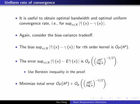
Uniform rate of convergence
• It is useful to obtain optimal bandwidth and optimal uniformconvergence rate, i.e., for supx∈X |γ (x)− γ (x) |.
• Again, consider the bias-variance tradeoff.
• The bias supx∈X |γ (x)− γ (x) | for rth order kernel is OP(hp).
• The error supx∈X |γ (x)− E γ (x) | is Op
((nhd
log n
)−1/2).
• Use Berstein inequality in the proof.
• Minimize total error OP(hp) + Op
((nhd
log n
)−1/2).
Han Hong Basic Nonparametric Estimation


3 Density Estimation
• Let h denote the length of the cells in the his-togram
• Let f denote the density and F the cdf, then:
f(x0) = limh→0
F (x0 + h)− F (x0 − h)
2h
• A first (naive) estimator of a density would be touse the height of cells in a histogram.
bfHIST (x0) =1
N
NXi=1
1(x0 − h < xi < x0 + h)
2h
=1
Nh
NXi=1
1
21µ¯xi − x0
h
¯< 1

• This corresponds to the probability of falling intoa bin of length 2h.
• In practice, note that this estimate of the densitywill be discontinuous.
• A more desirable (and efficient!) way to estimatethe density would be to smooth out the disconti-
nuities.
• A kernel density estimator generalizes our his-
togram estimator to:
bf(x0) = 1
Nh
NXi=1
1
2Kµxi − x0
h
• where K takes the place of the indicator function
above.

• K is called a kernel function and h is smoothing
parameter called a bandwidth.
• We will make the following assumptions about thekernel function:
(i) K(z) is symmetric around 0
(ii)RK(z)dz = 1,
RzK(z)dz = 0,
R|K(z)| dz <∞
(iii) (a) eitherK(z) = 0 for |z| > z0 or (b) |z|K(z)→0 as |z|→∞
(iv)Rz2K(z)dz = κ <∞
• We will commonly assume that z ∈ [−1, 1] as anormalization on the domain in the case of (iii)
a.

• Some commonly used kernels are:
uniform 1 (|z| < 1)
Epanechnikov3
4(1− z2)× 1 (|z| < 1)
normal (2π)−1/2 exp(−z2/2)
• Note that as h is larger, larger weights are givento observations further away from x0.
• That is, larger values of h smooth the observa-tions more heavily.
• In an application, we will want h→ 0 as N →∞so that in the limit (at an appropriate rate).

• Thus, we only include observations in an arbi-trarily small neighborhood in our density estimatebf(x0).
• In choosing the bandwidth, we will face a tradeoffbetween the bias of bf(x0), denoted b(x0), and thevariance of bf(x0), denoted V[ bf(x0)].
b(x0) = E[ bf(x0)]− f(x0) =1
2h2f 00(x0)
Zz2K(z)dz
V [ bf(x0)] = 1
Nhf(x0)
ZK(z)2dz + o(
1
Nh)
• Note that a small h decreases the bias but in-
creases the variance.
• In the limit, we it is desirable to let h → 0 and
Nh→∞ so that both the bias and the variance
eventually become zero.

• It can be shown that bf(x0) is pointwise consistentif h→ 0 and Nh→∞
• Uniform consistency if Nh/lnN → ∞ (this re-
quires more smoothing).
• It can be shown that the kernel is (pointwise)asymptotically normal,
(Nh)1/2³ bf(x0)− f(x0)− b(x0)
´→d N [0, f(x0)
ZK(z)2dz]
• This is potentially complicated object to com-pute.
• A practical alternative is to use a resampling pro-cedure such as the bootstrap.

• Another important choice is the bandwidth.
• This can be found by minimizing the expectedmean square error.
• There are also plug in estimates (such as Silvver-man’s plug in estimate).
4 Example-Part 1.
• Next, we consider the problem of the identifica-
tion and estimation of auction models.
• In an auction, the economist sees the distributionof bids.

• The economist wishes to infer bidder’s private in-formation and utility functions.
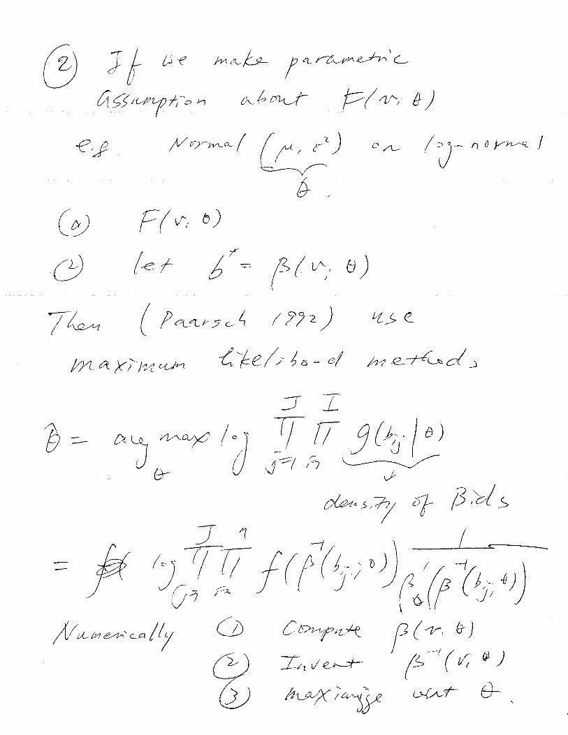
• Key papers in the literature are Paarsch (1992),Elyakime, Laffont, Loisel and Vuong (1994) and
Guerre, Perrigne and Vuong (2000).

5 First Price Auction Examples.
• Consider the first price auction with independentprivate values.
• In the model, there are i = 1, ..., N symmetricbidders with valuation vi for a single and indivis-ible object.
• Valuations are iid with cdf F (v) and pdf f(v).
• In the auction, bidders simultaneously submit sealedbids bi.
• Bidder i’s vNM utility is
ui(b1, ..., bn, vi) ≡(vi − bi if bi > bj for all i 6= j
0 otherwise.
(1)

• Let πi(bi; vi) denote the expected profit of bidderi where φ is the inverse of the bid function:
πi(bi; vi) ≡ (vi − bi)F (φ(b))N−1. (2)
• The first order condition for maximizing expectedprofits (2) implies that
v = b+F (φ(b))
f(φ(b))φ0(b)(N − 1). (3)
• This looks hard to deal with.
• Guerre, Perrigne and Vuong (2000) propose analternative approach.

• The econometrician observes t = 1, ..., T inde-
pendent replications of the auction described above.
• For each auction t, the econometrician observes
all of the bids bi,t.
• The object that GPV wish to estimate is F (v).
• Let G(b) = F (φ(bi)) denote the equilibrium dis-
tribution of the bids.

• If we substitute G(b) into (??) allows us to writeexpected utility as:
(vi − bi)G(bi)N−1.
The first order conditions can now be written as:
(vi − bi) (N − 1) g(bi)−G(bi) = 0 (4)
vi = bi +G(bi)
(N − 1)g(bi)(5)
• Let bG and bg denote estimates of G and g
• we can form an estimate bvi,t of bidder i’s privateinformation vi,t in auction t by substituting these
terms into (5):

bvi,t = bi,t +bG(bi,t)
(N − 1)bg(bi,t) (6)
To summarize, the estimator proposed by GPV:
1. Given bids bi,t for i = 1, ..., N and t = 1, ..., T ,
estimate the distribution and density of bids bG(b)and bg(b).
2. Compute bvi,t for i = 1, ..., N and t = 1, ..., T
using equation (6). Use the empirical cdf of thebvi,t to estimate F.

• This idea turns out to be quite general.
• The distribution of bids can be used to recoverprivate information even in multiple unit auctions
or auctions with dynamics.
• These estimators have been applied to offshore oildrilling, procurement, electronic commerce and
treasury bill markets.
• There are still some interesting research questionsleft, however, particularly in the common values
case.


Random Sample Generation and Simulation
of Probit Choice Probabilities
Based on sections 9.1-9.2 and 5.6 of Kenneth Train'sDiscrete Choice Methods with Simulation
Presented by Jason Blevins
Applied Microeconometrics Reading Group
Duke University
21 June 2006
Anyone attempting to generate random numbers by deterministic
means is, of course, living in a state of sin.
John Von Neumann, 1951

Outline
Density simulation and sampling
Univariate
Truncated univariate
Multivariate Normal
Accept-Reject Method for truncated densities
Importance sampling
Gibbs sampling
The Metropolis-Hastings Algorithm
Simulation of Probit Choice Probabilities
Accept-Reject Simulator
Smoothed AR Simulators
GHK Simulator
1

Simulation in Econometrics
Goal: approximate a conditional expectation which lacks a closed form.
Statistic of interest: t(), where F .
Want to approximate E [t()] =∫t()f ()d.
Basic idea: calculate t() for R draws of and take the average.
Unbiased: E[1R
∑Rr=1 t(
r)]= E [t()]
Consistent: 1R
∑Rr=1 t(
r)p
! E [t()]
This is straightforward if we can generate draws from F .
In discrete choice models we want to simulate the probability that agent nchooses alternative i .
Utility: Un;j = Vn;j + n;j with n F (n).
Bn;i = fn j Vn;i + n;i > Vn;j + n;j 8j 6= ig.
Pn;i =∫1Bn;i
(n) f (n)dn.
2

Random Number Generators
True Random Number Generators:
Collect entropy from system (keyboard, mouse, hard disk, etc.)
Unix: /dev/random, /dev/urandom
Pseudo-Random Number Generators:
Linear Congruential Generators (xn+1 = axn + b mod c): fast butpredictable, good for Monte Carlo
Nonlinear: more dicult to determine parameters, used in cryptography
Desirable properties for Monte Carlo work:
Portability
Long period
Computational simplicity
DIEHARD Battery of Tests of Randomness, Marsaglia (1996)
3
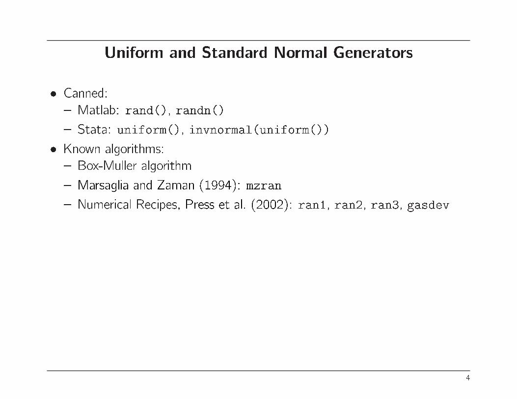
Uniform and Standard Normal Generators
Canned:
Matlab: rand(), randn()
Stata: uniform(), invnormal(uniform())
Known algorithms:
Box-Muller algorithm
Marsaglia and Zaman (1994): mzran
Numerical Recipes, Press et al. (2002): ran1, ran2, ran3, gasdev
4

Simulating Univariate Distributions
Direct vs. indirect methods.
Transformation
Let u N (0; 1). Then v = + u N(; 2
)and
w = e+u Lognormal(; 2
).
Inverse CDF transformation:
Let u N (0; 1). If F () is invertible, then = F1(u) F ().
Only works for univariate distributions
5

6

Truncated Univariate Distributions
Want to draw from g( j a b).
Conditional density in terms of unconditional distribution f ():
g( j a b) =
f ()
F (b)F (a); if a b
0; otherwise
Drawing is analogous to using the inverse CDF transformation.
Let U (0; 1) and dene = (1 )F (a) + F (b). = F1() isnecessarily between a and b.
7

8

The Multivariate Normal Distribution
Assuming we can draw from N (0; 1), we can generate draws from anymultivariate normal distribution N (;).
Let LL> be the Cholesky decomposition of and let N (0; I).
Then, since a linear transformation of a Normal r.v. is also Normal:
= + L N (;)
E [] = + LE [] =
Var () = E[(L)(L)>
]= E
[L>L>
]= LE
[>
]L>
= LVar ()L> =
9

The Accept-Reject Method for Truncated Densities
Want to draw from a multivariate density g(), but truncated so that a b with a; b; 2 Rl .
The truncated density is f () = 1kg() for some normalizing constant k .
Accept-Reject method:
Draw r from f ().
Accept if a r b, reject otherwise.
Repeat for r = 1; : : : ; R.
Accept on average kR draws.
If we can draw from f , then we can draw from g without knowing k .
Disadvantages:
Size of resulting sample is random if R is xed.
Hard to determine required R.
Positive probability that no draws will be accepted.
Alternatively, x the number of draws to accept and repeat until satised.
10

Importance Sampling
Want to draw from f but drawing from g is easier.
Transform the target expectation into an integral over g:∫t()f ()d =
∫t()
f ()
g()g()d:
Importance Sampling: Draw r from g and weight by f (r )g(r ).
The weighted draws constitute a sample from f .
The support of g must cover that of f and sup fg must be nite.
To show equivalence, consider the CDF of the weighted draws:∫f ()
g()1 ( < m) g()d =
∫ m
1
f ()
g()g()d
=
∫ m
1
f ()d = F (m)
11

The Gibbs Sampler
Used when it is dicult to draw from a joint distribution but easy to drawfrom the conditional distribution.
Consider a bivariate case: f (1; 2).
Drawing iteratively from conditional densities converges to draws from thejoint distribution.
The Gibbs Sampler: Choose an initial value 01.
Draw 02 f2(2 j 01), 11 f1(1 j
02); : : : , t1 f1(1 j
t12 ), t2
f2(2 j t1).
The sequence of draws f(01; 02); : : : ; (
t1;
t2)g converges to draws from
f (1; 2).
See Casella and George (1992) or Judd (1998).
12

The Gibbs Sampler: Example
1; 2 N (0; 1).
Truncation: 1 + 2 m.
Ignoring truncation,1 j 2 N (0; 1).
Truncated univariate sampling:
U (0; 1)
= (1 )(0) + (m 2)
1 = 1 ((m 2))
13

The Metropolis-Hastings Algorithm
Only requires being able to evaluate f and draw from g.
Metropolis-Hastings Algorithm:
1. Let 0 be some initial value.2. Choose a trial value ~1 = 0 + , g(), where g has zero mean.3. If f (~1) > f (0), accept ~1.4. Otherwise, accept ~1 with probability f (~1)=f (0).5. Repeat for many iterations.
The sequence ftg converges to draws from f .
Useful for sampling truncated densities when the normalizing factor isunknown.
Description of algorithm: Chib and Greenberg (1995)
14

Calculating Probit Choice Probabilities
Probit Model:
Utility: Un;j = Vn;j + n;j with n N (0;).
Bn;i = fn j Vn;i + n;i > Vn;j + n;j 8j 6= ig.
Pn;i =∫Bn;i
(n)dn.
Non-simulation methods:
Quadrature: approximate the integral using a specically chosen set ofevaluation points and weights (Geweke, 1996, Judd, 1998).
Clark algorithm: maximum of several normal r.v. is itself approximatelynormal (Clark, 1961, Daganzo et al., 1977).
Simulation methods:
Accept-reject method
Smoothed accept-reject
GHK (Geweke-Hajivassiliou-Keane)
15

The Accept-Reject Simulator
Straightforward:
1. Draw from distribution of unobservables.2. Determine the agent's preferred alternative.3. Repeat R times.4. The simulated choice probability for alternative i is the proportion of times
the agent chooses alternative i .
General:
Applicable to any discrete choice model.
Works with any distribution that can be drawn from.
16

The Accept-Reject Simulator for Probit
Let Bn;i = fn j Vn;i + n;i > Vn;j + n;j ; 8j 6= ig. The Probit choiceprobabilities are:
Pn;i =
∫1Bn;i
(n)(n)dn:
Accept-Reject Method:
1. Take R draws f1n; : : : ; Rn g from N (0;) using the Cholesky
decomposition LL> = to transform iid draws from N (0; 1).2. Calculate the utility for each alternative: Ur
n;j = Vn;j + rn;j .3. Let d r
n;j = 1 if alternative j is chosen and zero otherwise.4. The simulated choice probability for alternative i is:
Pn;i =1
R
R∑r=1
d rn;i
17

The Accept-Reject Simulator: Evaluation
Main advantages: simplicity and generality.
Can also be applied to the error dierences in discrete choice models.
Slightly faster
Conceptually more dicult
Disadvantages:
Pn;i will be zero with positive probability.
Pn;i is a step function and the simulated log-likelihood is not dierentiable.
Gradient methods are likely to fail (gradient is either 0 or undened).
18

19
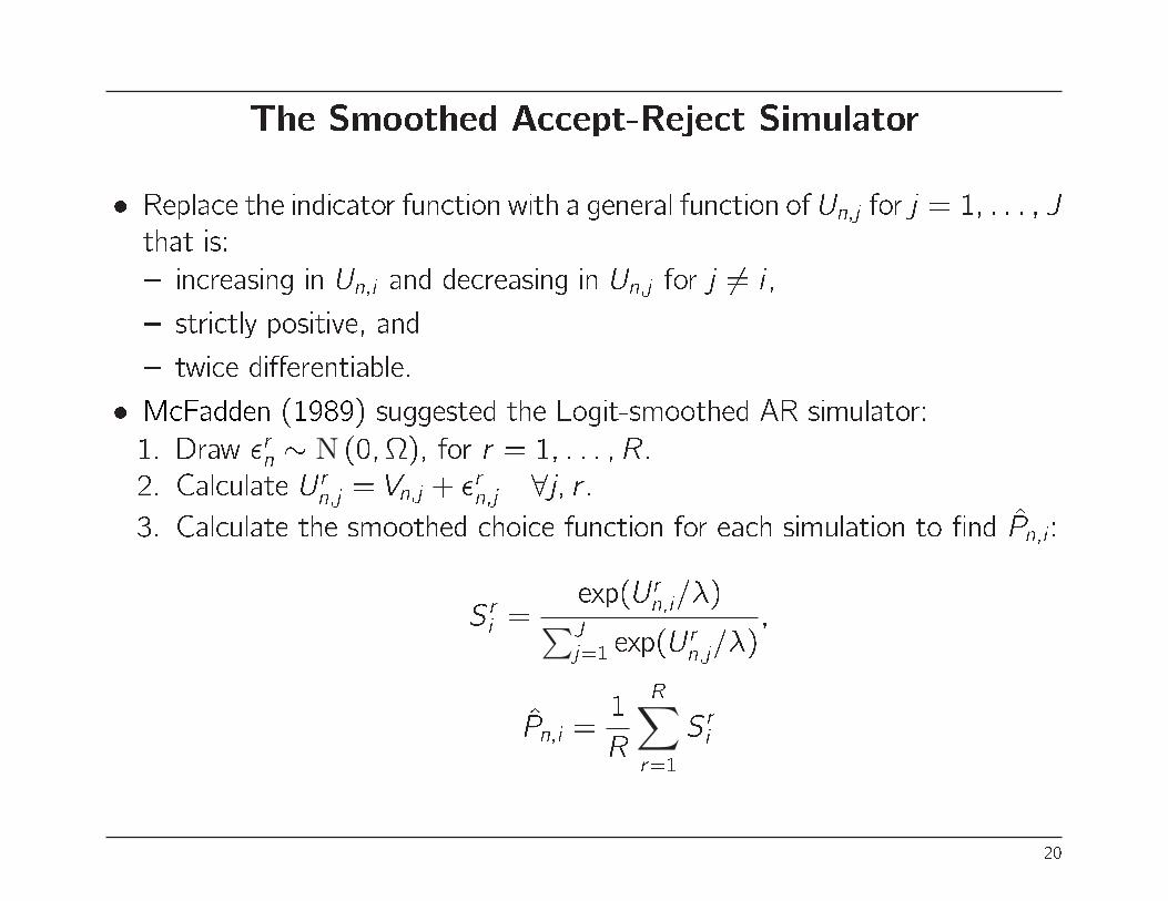
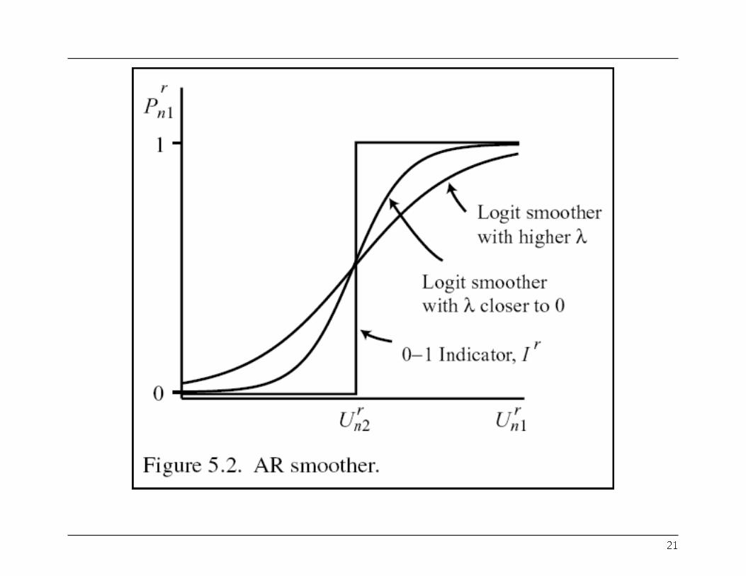
The Smoothed Accept-Reject Simulator
Replace the indicator function with a general function of Un;j for j = 1; : : : ; Jthat is:
increasing in Un;i and decreasing in Un;j for j 6= i ,
strictly positive, and
twice dierentiable.
McFadden (1989) suggested the Logit-smoothed AR simulator:
1. Draw rn N (0;), for r = 1; : : : ; R.2. Calculate Ur
n;j = Vn;j + rn;j 8j; r .
3. Calculate the smoothed choice function for each simulation to nd Pn;i :
Sri =
exp(Urn;i=)∑J
j=1 exp(Urn;j=)
;
Pn;i =1
R
R∑r=1
Sri
20
21

The Smoothed Accept-Reject Simulator: Evaluation
Simulated log-likelihood using smoothed choice probabilities is... smooth.
Slightly more dicult to implement than AR simulator.
Can provide a behavioral interpretation.
Choice of smoothing parameter is arbitrary.
Objective function is modied.
Use alternative optimization methods instead (simulated annealing)?
22

The GHK Simulator
GHK: Geweke, Hajivassiliou, Keane.
Simulates the Probit model in dierenced form.
For each i , simulation of Pn;i uses utility dierences relative to Un;i .
Basic idea: write the choice probability as a product of conditionalprobabilities.
We are much better at simulating univariate integrals over N(0; 1) thanthose over multivariate normal distributions.
23

GHK with Three Alternatives
An example with three alternatives:
Un;j = Vn;j + n;j ; j = 1; 2; 3 with n N (0;)
Assume has been normalized for identication.
Consider Pn;1. Dierence with respect to Un;1:
~Un;j;1 = ~Vn;j;1 + ~n;j;1; j = 2; 3 with ~n;1 N(0; ~1
)Pn;1 = P
(~Un;2;1 < 0; ~Un;3;1 < 0
)= P
(~Vn;2;1 + ~n;2;1 < 0; ~Vn;3;1 + ~n;3;1 < 0
) Pn;1 is still hard to evaluate because ~n;j;1's are correlated.
24

GHK with Three Alternatives
One more transformation. Let L1L>
1 be the Cholesky decomposition of ~1:
L1 =
(caa 0cab cbb
) Then we can express the errors as:
~n;2;1 = caa1
~n;3;1 = cab1 + cbb2
where 1; 2 are iid N (0; 1).
The dierenced utilities are then
~Un;2;1 = ~Vn;2;1 + caa1
~Un;3;1 = ~Vn;3;1 + cab1 + cbb2
25
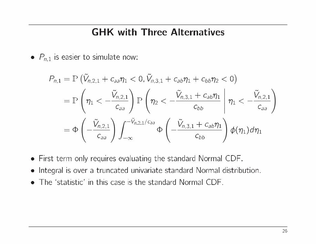
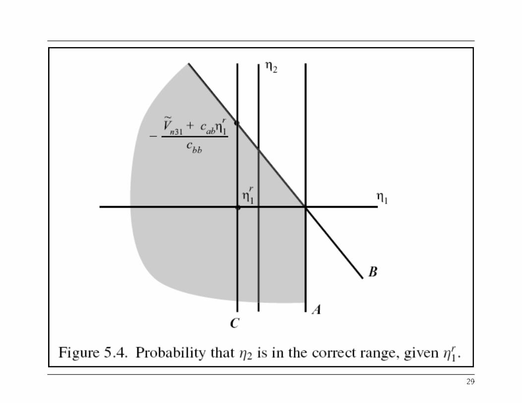
GHK with Three Alternatives
Pn;1 is easier to simulate now:
Pn;1 = P(~Vn;2;1 + caa1 < 0; ~Vn;3;1 + cab1 + cbb2 < 0
)= P
(1 <
~Vn;2;1caa
)P
(2 <
~Vn;3;1 + cab1cbb
∣∣∣∣∣ 1 < ~Vn;2;1caa
)
=
(~Vn;2;1caa
)∫~Vn;2;1=caa
1
(~Vn;3;1 + cab1
cbb
)(1)d1
First term only requires evaluating the standard Normal CDF.
Integral is over a truncated univariate standard Normal distribution.
The `statistic' in this case is the standard Normal CDF.
26

27

GHK with Three Alternatives: Simulation
(~Vn;2;1caa
)∫
~Vn;2;1caa
1
(~Vn;3;1 + cab1
cbb
)(1)d1 = k
∫ 1
1
t(1)(1)d1
1. Calculate k = (
~Vn;2;1caa
).
2. Draw r1 from N (0; 1) truncated at ~Vn;2;1=caa for r = 1; : : : ; R: Draw
r U (0; 1) and calculate r1 = 1
(r
(
~Vn;2;1caa
)).
3. Calculate t r = (
~Vn;3;1+cabr1
cbb
)for r = 1; : : : ; R.
4. The simulated choice probability is Pn;1 = k 1R
∑Rr=1 t
r
28
29

GHK as Importance Sampling
Pn;1 =
∫1B () g()d
where B = f j ~Un;j;i < 0 8j 6= ig and g() is the standard Normal PDF.
Direct (AR) simulation involves drawing from g and calculating 1B ().
GHK draws from a dierent density f () (the truncated normal):
f () =
(1)
(~Vn;1;i=c11)
(2)
((~Vn;2;i+c211)=c22) ; if 2 B
0; otherwise
Dene Pi ;n() = (~Vn;1;i=c11)((~Vn;2;i + c211)=c22) .
f () = g()=Pn;i() on B.
Pn;i =∫1B () g()d =
∫1B ()
g()
g()=Pi ;n()f ()d =
∫Pi ;n()f ()d
30

References
George Casella and Edward I. George. Explaining the gibbs sampler. The American Statistician, 46:167174,
1992.
Siddhartha Chib and Edward Greenberg. Understanding the Metropolis-Hastings algorithm. The American
Statistician, 49:327335, 1995.
Charles E. Clark. The greatest of a nite set of random variables. Operations Research, 9:145162, 1961.
Carlos F. Daganzo, Fernando Bouthelier, and Yosef She. Multinomial probit and qualitative choice: A
computationally ecient algorithm. Transportation Science, 11:338358, 1977.
John Geweke. Monte Carlo simulation and numerical integration. In Hans M. Amman, David A. Kendrick,
and John Rust, editors, Handbook of Computational Economics, volume 1, Amsterdam, 1996. North
Holland.
Kenneth L. Judd. Numerical Methods in Economics. MIT Press, Cambridge, MA, 1998.
George Marsaglia. DIEHARD: A battery of tests of randomness. http://www.csis.hku.hk/~diehard,
1996.
George Marsaglia and Arif Zaman. Some portable very-long-period random number generators. Computers
in Physics, 8:117121, 1994.
Daniel McFadden. A method of simulated moments for estimation of discrete response models without
numerical integration. Econometrica, 57:9951026, 1989.
William H. Press, William T. Vetterling, Saul A. Teukolsky, and Brian P. Flannery. Numerical Recipes in
C++: The Art of Scientic Computing. Cambridge University Press, 2002.
31

Markov Chain Monte Carlo Methods
John Geweke
Department of EconomicsUniversity of Iowa
Presentation at ICE 06, Chicago, July, 2006
Part I

The Central Idea
• θ(m) ∼ p(θ|θ(m−1),C
), (m = 1, 2, 3, . . .)
• If C is specified correctly, then
θ(m−1) ∼ p (θ|I ) , θ(m) ∼ p(θ|θ(m−1),C
)=⇒ θ(m) ∼ p (θ|I ) .
• Better yet, if
θ(m−1) ∼ p (theta|J) , θ(m) ∼ p(θ|θ(m−1),C
)=⇒ θ(m) ∼ p (θ|J)
then J = I . And even better,
p(θ(m)|θ(0),C
)d−→ p (θ|I ) , ∀θ(0) ∈ Θ.

The central idea continued
• If p(θ(m)|θ(0),C
) d−→ p (θ|I ) , ∀θ(0) ∈ Θ, then we canapproxiate E [h (ω) |I ] by
• iterating the chain B (“burn-in”) times:
• drawing ω(m) ∼ p(ω|θ(m)
), (m = 1, . . . ,M);
• Computing
hM = M−1M∑
m=1
h(ω(m)
).

The Gibbs sampler
• Blocking: θ′ =(θ′(1), . . . , θ
′(B)
).
• Some notation: corresponding to any subvector θ(b),
θ′<(b) =(θ′(1), . . . , θ
′(b−1)
), (b = 2, . . . ,B) , θ<(1) = ∅
θ′>(b) =(θ′(b+1), . . . , θ
′(B)
), (b = 1, . . . ,B − 1) , θ>(B) = ∅
θ′−(b) =(θ′<(b), θ
′>(b)
)• Very important: choose the blocking so that
θ(b) ∼ p(θ(b)|θ−(b), I
)is possible.

Intuitive argument for the Gibbs sampler
Imagine θ(0) ∼ p (θ|I ), and then in succession
θ(1)(1) ∼p
(θ(1)|θ
(0)−(1), I
),
θ(1)(2) ∼p
(θ(2)|θ
(1)<(2), θ
(0)>(2), I
),
θ(1)(3) ∼p
(θ(3)|θ
(1)<(3), θ
(0)>(3), I
),
...,
θ(1)(b) ∼p
(θ(b)|θ
(1)<(b), θ
(0)>(b), I
),
...,
θ(1)(B) ∼p
(θ(B)|θ
(1)<(B), θ
(0)>(B), I
)We have θ(1) ∼ p (θ|I ).

Now repeat
θ(2)(1) ∼p
(θ(1)|θ
(1)−(1), I
),
θ(2)(2) ∼p
(θ(2)|θ
(2)<(2), θ
(1)>(2), I
),
θ(2)(3) ∼p
(θ(3)|θ
(2)<(3), θ
(1)>(3), I
),
...
θ(2)(b) ∼p
(θ(b)|θ
(2)<(b), θ
(1)>(b), I
),
...
θ(2)(B) ∼p
(θ(B)|θ
(2)<(B), θ
(1)>(B), I
).
We have θ(2) ∼ p (θ|I ).

• The general step in the Gibbs sampler is
θ(m)(b) ∼p
(θ(b)|θ
(m)<(b), θ
(m−1)>(b) , I
)for b = 1, . . . ,B and m = 1, 2, . . .
• This defines the Markov chain
p(θ(m)|θ(m−1),G
)=
B∏b=1
p[θ
(m)(b) |θ
(m)<(b), θ
(m−1)>(b) , I
].
• Key property:
θ(0) ∼ p (θ|I )⇒ θ(m) ∼ p (θ|I ) .
• Potential problems: disjoint support.

The Metropolis-Hastings Algorithm
• What it does: θ∗ ∼ q(θ∗|θ(m−1),H
)• Then
P(θ(m) = θ∗
)=α
(θ∗|θ(m−1),H
)P(θ(m) = θ(m−1)
)=1− α
(θ∗|θ(m−1),H
)where
α(θ∗|θ(m−1),H
)= min
p (θ∗|I ) /q
(θ∗|θ(m−1),H
)p(θ(m−1)|I
)/q(θ(m−1)|θ∗,H
) , 1.

Some aspects of the Metropolis-Hastings algorithm
• If we define
u (θ∗|θ,H) = q (θ∗|θ,H)α (θ∗|θ,H)
• then
P(θ(m) = θ(m−1)|θ(m−1) = θ,H
)=r (θ|H)
=1−∫
Θu (θ∗|θ,H) dν (θ∗) .
• Notice that
P(θ(m) ∈ A|θ(m−1) = θ,H
)=
∫A
u (θ∗|θ,H) dν (θ∗) + r (θ|H) IA (θ) .

u (θ∗|θ,H) = q (θ∗|θ,H)α (θ∗|θ,H)
We can write the transition density in one line making use of theDirac delta function, an operator with the property∫
Aδθ (θ∗) f (θ∗) dν (θ∗) = f (θ) IA (θ)
Then
p(θ(m)|θ(m−1),H
)=u(θ(m)|θ(m−1),H
)+ r
(θ(m−1)|H
)δθ(m−1)
(θ(m)
).

Special case of the Metropolis-Hastings algorithm
α(θ∗|θ(m−1),H
)= min
p (θ∗|I ) /q
(θ∗|θ(m−1),H
)p(θ(m−1)|I
)/q(θ(m−1)|θ∗,H
) , 1
• Special case 1, original Metropolis (1953):
q (θ∗|θ,H)
=⇒ α(θ∗|θ(m−1),H
)= min [p (θ∗|I ) , 1]
• Important example: random walk Metropolos chain
q (θ∗|θ,H) = q (θ∗ − θ|H) ,
where q (·|H) is symmetric about zero.

Special cases of the Metropolis-Hastings algorithm
α(θ∗|θ(m−1),H
)= min
p (θ∗|I ) /q
(θ∗|θ(m−1),H
)p(θ(m−1)|I
)/q(θ(m−1)|θ∗,H
) , 1
• Special case 2, Metropolis independence chain:
q (θ∗|θ,H) = q (θ∗|H)
=⇒ α(θ∗|θ(m−1),H
)= min
p (θ∗|I ) /q (θ∗|H)
p(θ(m−1)|I
)/q(θ(m−1)|H
) , 1
= min
w (θ∗)
w(θ(m−1)
) , 1
where w (θ) = p (θ|I ) /q (θ|H).
Why does the Metropolis-Hastings algorithm work?
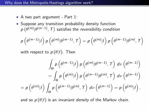
• A two part argument - Part 1:
• Suppose any transition probability density functionp(θ(m)|θ(m−1),T
)satisfies the reversibility condition
p(θ(m−1)|I
)p(θ(m)|θ(m−1),T
)= p
(θ(m)|I
)p(θ(m−1)|θ(m),T
)with respect to p (θ|I ). Then∫
Θp(θ(m−1)|I
)p(θ(m)|θ(m−1),T
)dν(θ(m−1)
)=
∫Θp(θ(m)|I
)p(θ(m−1)|θ(m),T
)dν(θ(m−1)
)= p
(θ(m)|I
)∫Θp(θ(m−1)|θ(m),T
)dν(θ(m−1)
)= p
(θ(m)|I
).
and so p (θ|I ) is an invariant density of the Markov chain.

• Part 2 of the argument (How Hastings did it):
• Suppose we don’t know the probability α(θ∗|θ(m−1),H
), but
we want p(θ(m)|θ(m−1),H
)to be reversible with respect to
p (θ|I ):
•
p(θ(m−1)|I
)p(θ(m)|θ(m−1),H
)= p
(θ(m)|I
)p(θ(m−1)|θ(m),H
).
• Trivial if θ(m−1) = θ(m). For θ(m−1) 6= θ(m) we need
p(θ(m−1)|I
)q(θ∗|θ(m−1),H
)α(θ∗|θ(m−1),H
)= p (θ∗|I ) q
(θ(m−1)|θ∗,H
)α(θ(m−1)|θ∗,H
).

•
p(θ(m−1)|I
)q(θ∗|θ(m−1),H
)α(θ∗|θ(m−1),H
)= p (θ∗|I ) q
(θ(m−1)|θ∗,H
)α(θ(m−1)|θ∗,H
).
• Suppose without loss of generality that
p(θ(m−1)|I
)q(θ∗|θ(m−1),H
)> p (θ∗|I ) q
(θ(m−1)|θ∗,H
).
• Set α(θ(m−1)|θ∗,H
)= 1 and
α(θ∗|θ(m−1),H
)=
p (θ∗|I ) q(θ(m−1)|θ∗,H
)p(θ(m−1)|I
)q(θ∗|θ(m−1),H
) .

Why does the Metropolis-Hastings algorithm work?
• The goal is to verify the reversibility condition:
f (x) f(x ′|x
)= f
(x ′)f(x |x ′
)• Note that according to the Gibbs sampler:
f(x ′|x
)=
∫f(x ′|y
)f (y |x) dy =
∫f (x ′, y) f (x , y)
f (y) f (x)dy .
• Therefore
f (x) f(x ′|x
)=f (x)
∫f(x ′|y
)f (y |x) dy
=
∫f (x ′, y) f (x , y)
f (y)dy .
• This is obviously exchangable in x and x ′. Hence thereversibility condition holds.

Lecture 6, Bayes Estimators
Department of EconomicsStanford University
September, 2008

Bayesian methods
• Prior π (θ). likelihood f (x|θ).
• Posterior density
p (θ|x) =f (x|θ)π (θ)∫f (x|θ)π (θ) dθ
.
• In general, computing p (θ|x) is difficult.
• Exception: conjugate family. Let F denote the class oflikelihoods f (x|θ). A class Π of prior distributions is aconjugate family for F if the posterior distribution is in theclass Π for all f ∈ F , all priors in Π, and all x ∈ X .
• The conjugate family for the normal mean when variances areknown is normal.

• Xt, t = 1, . . . , n i.i.d. Xt ∼ N(µ, σ2
). σ2 known.
• Prior π (µ) ∼ N (µ0, λ0), µ0, λ0 known.
• Posterior distribution
p (µ|X) ∼ N
(λ2x + σ2
n µ0
λ2 + σ2
n
,σ2
n λ2
λ2 + σ2
n
).
• Write t0 = 1/λ2, t = n/σ2: precision parameters.
p (µ|X) ∼ N
(t0µ0 + t x
t0 + t,
1
t0 + t
)• prior mean and sample mean are weighted by their precisions.
• Posterior precision sum of prior and data precisions.

• Bayesian point estimator.
• minimizes posterior expected loss functions:
θ = minθ∈Θ
∫ρ(θ − θ
)p(θ|x)d θ.
• If ρ (x) = x2, square loss:
θ =
∫θp(θ|x)d θ posterior mean.
• In the normal example:
µ =t0µ0 + t x
t0 + t.
• Other posterior locations, or loss functions, can be used.
• Posteriot interval: region under p (θ|x) with a given area.

No frequentists shall be denied the pleasure ofBayesian techniques
Department of EconomicsStanford University
November, 2011


Lecture 11: Bootstrap
Instructor: Han Hong
Department of EconomicsStanford University
2011
Han Hong Bootstrap

The Bootstrap Principle
• Replace the real world by the bootstrap world:
• Real World: Population(F0) −→ Sample(F1): X1, . . . ,Xn.
• The bootstrap world: Sample(F1): X1, . . . ,Xn −→ BootstrapSample F2 = X ∗1 , . . . ,X
∗n .
• We care about functional of F0 : θ (F0), the bootstrapprinciple says that we estimate θ (F0) by θ (F1).
• The only problem is how to define θ (F0), and the bootstrapresample is only useful for defining this function for θ (F1).
• A bootstrap resample is a sample of size n, drawnindependently with replacement from the empiricaldistribution F1, i.e., P (X ∗i = Xj |F1) = n−1, 1 ≤ i , j ≤ n.
Han Hong Bootstrap
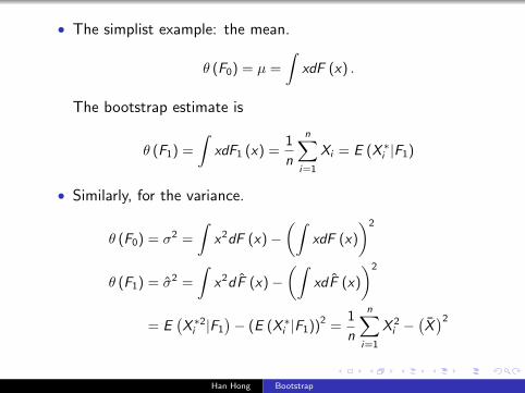
• The simplist example: the mean.
θ (F0) = µ =
∫xdF (x) .
The bootstrap estimate is
θ (F1) =
∫xdF1 (x) =
1
n
n∑i=1
Xi = E (X ∗i |F1)
• Similarly, for the variance.
θ (F0) = σ2 =
∫x2dF (x)−
(∫xdF (x)
)2
θ (F1) = σ2 =
∫x2dF (x)−
(∫xdF (x)
)2
= E(X ∗2i |F1
)− (E (X ∗i |F1))2 =
1
n
n∑i=1
X 2i −
(X)2
Han Hong Bootstrap
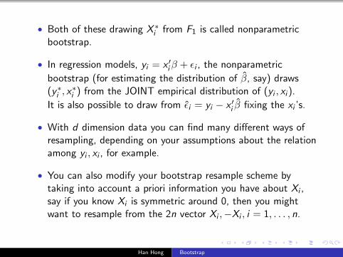
• Both of these drawing X ∗i from F1 is called nonparametricbootstrap.
• In regression models, yi = x ′iβ + εi , the nonparametric
bootstrap (for estimating the distribution of β, say) draws(y∗i , x
∗i ) from the JOINT empirical distribution of (yi , xi ).
It is also possible to draw from εi = yi − x ′i β fixing the xi ’s.
• With d dimension data you can find many different ways ofresampling, depending on your assumptions about the relationamong yi , xi , for example.
• You can also modify your bootstrap resample scheme bytaking into account a priori information you have about Xi ,say if you know Xi is symmetric around 0, then you mightwant to resample from the 2n vector Xi ,−Xi , i = 1, . . . , n.
Han Hong Bootstrap

Parameteric Bootstrap
• If you know F0 is from a parametric family, say E(λ = µ−1
),
then you may want to resample from F (λ) = E(λ) instead ofthe empirical distribution F1.
• If you choose MLE, then it is λ = 1µ = 1
X. So you resample
from an exponential distribution with mean X .
• But we will only discuss nonparametric bootstrap today.
• The bootstrap principle again: The whole business is to findthe definition of the functional θ (F0).
• It is often the solution t = θ (F0) to E [f (F1,F0; t) |F0] = 0.
• Since we don’t know F0, the bootstrap version is to estimate tby t s.t. E
[f(F2,F1; t
)|F1
]= 0.
• Examples are bias reduction and confidence interval.
Han Hong Bootstrap

Bias Reduction
• Need t = E (θ (F1)− θ (F0) |F0). The bootstrap principlesuggests estimating by t = E (θ (F2)− θ (F1) |F1).
• For example,θ (F0) = µ2 =
(∫xdF0 (x)
)2, then θ (F1) = X 2 =
(∫xdF1 (x)
)2.
E (θ (F1) |F0) = EF0
(µ+ n−1
n∑i=1
[Xi − µ]
)2
= µ2 + n−1σ2
=⇒ t = n−1σ2 = O(n−1)
E (θ (F2) |F1) = EF1
(X + n−1
n∑i=1
[X ∗i − X
])2
= X 2 + n−1σ2
=⇒ t = n−1σ2 where σ2 = n−1n∑
i=1
(Xi − X
)2
Han Hong Bootstrap

• So the bootstrap bias-corrected estimate of µ2 is:
θ (F1)− t = 2θ (F1)− E (θ (F2) |F1) = X 2 − n−1σ2
Its bias is:
E[X 2 − n−1σ2 − µ2|F0
]= n−1σ2 − n−1
(1− n−1
)σ2 = n−2σ2
So the bias is reduced by an order of O(n−1), compared to
the uncorrected estimate.
• For this problem, the one step bootstrap bias correction doesnot completely eliminate the bias.(It turns out bootstrapiteration will do)
• But another resample scheme, the jacknife, can eliminate biascompletely for this example.
Han Hong Bootstrap

Jacknife
• In general, let θ be an estimator using all data and θ−i be theestimator obtained by omitting observation i .
• The ith jacknife pseudovalue is given as θ∗i = nθ− (n − 1) θ−i .
• The Jacknife estimator is the average of these n of θ∗i :
θJ ≡ 1n
∑ni=1 θ
∗i .
• In this example, θ = X 2. θ−i =(
1n−1
∑j 6=i Xj
)2. So
θJ = nX 2 − (n − 1)
1
n − 1
∑j 6=i
Xj
2
which is unbiased.
Han Hong Bootstrap

Confidence Interval
• Look for a one-sided confidence interval of the form(−∞, θ + t) with coverage probability of α:
P(θ (F0) ≤ θ + t
)= α =⇒ P
(θ (F0)− t ≤ θ
)= α.
• The bootstrap version becomes P(θ (F1)− t ≤ θ (F2)
)= α. So
−t is (1− α)th quantile of θ (F2)− θ (F1) conditional on θ (F1).
• Usually the distribution function of θ (F2)− θ (F1) conditionalon F1 is difficult to calculate, as difficult as θ (F1)− θ (F0)conditional on θ (F0).
• But as least the former can be simulated (since you know F1),while the later can’t (since you don’t know F0).
Han Hong Bootstrap

• To simulate the distribution of θ (F2)− θ (F1) conditional on F1
(1) Independently draw B (a very big number, say 100,000)bootstrap resamples X ∗b , b = 1, . . . ,B from F1, where eachX ∗b = (X ∗b1, . . . ,Xbn)∗, each X ∗bi is independent draw from theempirical distribution.
(2) For each X ∗b , calculate θ∗b = θ (X ∗b ). Then simply use theempirical distribution of X ∗b , or any smoothed version of it, toapproximate the distribution of θ (F2)− θ (F1) conditional onF1.
This approximation can be arbitrary close as B →∞.
Han Hong Bootstrap

Distribution of Test Statistics
• Almost just the same as the confidence interval problem.
• Consider a statistics(like OLS coefficient β, t-statistics)Tn = Tn (X1, . . . ,Xn), want to know its distribution function:
Pn (x ,F0) = P (Tn ≤ x |X1, . . . ,Xn ∼ iid F0)
• But don’t know F0, so use the bootstrap principle,
Pn (x ,F1) = P (T ∗n ≤ x |X ∗1 , . . . ,X ∗n ∼ iid F1)
• Again when Pn (x ,F1) can’t be analytically computed, it canbe approximated arbitrary well by
Pn (x ,F1) ≈ 1
B
B∑b=1
1 (T ∗nb ≤ x)
for T ∗nb = Tn (X ∗b1, . . . ,X∗bn).
Han Hong Bootstrap

• Note again the schema in the bootstrap approximation.
Pn (x ,F0)1≈ Pn (x ,F1)
2≈ 1
B
B∑b=1
1 (T ∗nb ≤ x)
1 The statistical error: introduced by replacing F0 with F1, thesize of error as n→∞ can be analyzed through asymptotictheory, e.g. Edgeworth expansion.
2 The numerical error: introduced by approximating F1 usingsimulation. Should disappear as B →∞. It has nothing to dowith n-asymptotics and statistical error.
• Similarly, standard error of Tn
σ2 (Tn) ≈ σ2 (T ∗n ) ≈ 1
B
B∑b=1
(T ∗nb −
1
B
B∑b=1
T ∗nb
)2
Han Hong Bootstrap

The Pitfall of Bootstrap
• Whether the bootstrap works or not (in the consistency senseof whether P (T ∗n ≤ x |F1)− P (Tn ≤ x |F0) −→ 0) need to beanalyzed case by case.
•√n consistent, asymptotically normal test statistics can be
bootstrapped, but it is not known whether other things maywork.
• Example of inconsistency, nonparametric bootstrap fails.
Take F ∼ U (0, θ), and X(1), . . . ,X(n) is the order statistics ofthe sample, so X(n) is the maximum. It is naturally toestimate θ using X(n).
Han Hong Bootstrap

• θ−X(n)
θ converges at rate n to E (1), since for x > 0:
P
(nθ − X(n)
θ> x
)= P
(X(n) < θ − θx
n
)= P
(Xi < θ − θx
n
)n
=
(1
θ
(θ − θx
n
))n
=(
1− x
n
)n n→∞−→ e−x
In particular, the limiting distribution is continuous.
• But this is not the case for bootstrapped distribution, X ∗(n).
The bootstrapped version is naturally n(X(n) − X ∗(n))/X(n). But
P
(nX(n) − X ∗(n)
X(n)= 0
)=
(1−
(1− 1
n
)n)n→∞−→
(1− e−1
)≈ 0.63
So there is a big probability mass at 0 in the limitingdistribution of the bootstrap sample.
Han Hong Bootstrap

• It turns out that in this example parametric bootstrap wouldwork although nonparametric bootstrap fails. But there aremany examples where even parametric bootstrap will fail.
• An alternative to bootstrap, called subsample, proposed byRomano(1998), which include the jacknife as a special case, isalmost always consistent, as long as the subsample size msatisfies m→∞ and m/n→ 0. The jacknife case m = n − 1does not satisfy the general consistency condition. Serialcorrelation in time series also creates problem for naivenonparametric bootstrap. Subsample is one way out.
• The other alternative is to resample blocks instead ofindividual observations(Fitzenberg(1998)).
• However, both of these will only give consistency but not the2nd order benefit of edgeworth expansion.
Han Hong Bootstrap

• So if in most cases bootstrap only works when asymptotictheory works, why use bootstrap?
• Some conceivable benefits are:
• Don’t want to waste time deriving asymptotic variance,although
√n consistency and asym normality is known. Let
the computer do the job.
• Avoid bandwidth selection in estimating var-cov of quantileregression type estimators. Bandwidth is needed for eitherkernel estimate of the conditional density f (0|xt) or fornumerical derivatives.
• For asymptotic pivotal statistics, bootstrapping is equivalent toautomatically doing edgeworth expansion.
Han Hong Bootstrap

Exact Pivotal Statistics
• An exact (or asymptotic) pivotal statistics Tn is one whose (orasymptotic) distribution does not depend on unknownparameters ∀n.
• Denote pivotal statistics by Tn and nonpivotal ones by Sn.
• If know that F ∼ N(µ, σ2
), then
• Sn =√n(X − µ
)∼ N
(0, σ2
)is nonpivotal since unknown σ2.
The bootstrap estimate is N(0, σ2
), so there is error in
approximating the distribution of Sn.
• Tn =√n − 1
(X−µ)σ2 ∼ tn−1 for σ2 = 1
n
∑ni=1
(Xi − X
)2.
The bootstrap estimate is also tn−1. No error here.
• If Tn is exact pivotal, need not bootstrap at all. Either look upa table or simulate. But most statistics are asymptotic pivotal.
Han Hong Bootstrap

Asymptotic Pivotal Statistics
• No matter what F is, for t-statistics the CLT saysP (Tn ≤ x)
n→∞−→ Φ (x), so it is asymptotically pivotal.
• But the CLT doesn’t say how fast P (Tn ≤ x) tends to Φ (x).
• The Edgeworth expansion describes it:
Pn (x ,F0) ≡ P (Tn ≤ x |F0) = Φ (x) + G (x ,F0)1√n
+ O(n−1)
The bootstrap version is:
Pn (x ,F1) ≡ P (T ∗n ≤ x |F1) = Φ (x) + G (x ,F1)1√n
+ Op
(n−1)
• The Edgeworth expansion can be carried out up to manyterms in power of n−1/2. Expansion up to the 2nd term:
Pn (x ,F0) ≡ P (Tn ≤ x |F0) = Φ (x) + G (x ,F0)1√n
+ H (x ,F0)1
n+ O
(n−
32
)Han Hong Bootstrap

Consider error in approximating Pn (x ,F0):
• Error of CLT:
Pn (x ,F0)− Φ (x) = G (x ,F0) 1√n
+ O(n−1)
= O(
1√n
)• Error of Bootstrap:
Pn (x ,F0)− Pn (x ,F1) = G (x ,F0) 1√n− G (x ,F1) 1√
n+ Op
(n−1)
=
(G (x ,F0)− G (x ,F1)) 1√n
+ Op
(n−1)
= Op
(n−1)
since√n (F1 − F0) = Op (1), and assuming G (x ,F ) is smooth
and differentiable in the 2nd argument:
G (x ,F1)− G (x ,F0) = Op (F1 − F0) = Op
(1√n
).
• So if your sample size is 100, By CLT you commit an error of(roughly) 0.1, but by bootstrap 0.01, big improvement??
Han Hong Bootstrap

• However, this improvement doesn’t work for nonpitovalstatistics, say Sn: by CLT
P (Sn ≤ x)n→∞−→ Φ
( xσ
).
• The corresponding Edgeworth expansion is:
Pn (x ,F0) ≡ P (Sn ≤ x |F0) = Φ( xσ
)+ G (x/σ,F0)
1√n
+ O(n−1)
The bootstrap version is:
Pn (x ,F1) ≡ P (S∗n ≤ x |F1) = Φ( xσ
)+ G (x/σ,F1)
1√n
+ O(n−1)
Han Hong Bootstrap

Consider error in approximating Pn (x ,F0):
• Error of CLT: need to replace σ by σ.
Pn (x ,F0)− Φ (x/σ) =
Φ (x/σ)− Φ (x/σ) + G (x/σ,F0) 1√n
+ O(n−1)
= O(
1√n
)• Error of Bootstrap:
Pn (x ,F0)− Pn (x ,F1) = Φ (x/σ)− Φ (x/σ) + G (x/σ,F0) 1√n−
G (x/σ,F1) 1√n
+ Op
(n−1)
= Op
(n−1/2
)This is because both F1 − F0 = Op
(1√n
)and σ − σ = Op
(1√n
).
• No improvement compared to CLT. This is because now the1st term Φ (x/σ) does not cancelled with Φ (x/σ).
Han Hong Bootstrap

• The implication of this is that bootstrapping provides betterapproximation to two sided symmetric test(or symmetricconfidence interval) compared to one sided test(or confidenceinterval).
• Assume G (x ,F0) is an even function in x .
• One-sided test: reject if Tn ≤ x (or Tn > x), theapproximaton error being:
Pn (x ,F0)− Pn (x ,F1) = G (x ,F0)1√n− G (x ,F1)
1√n
+ Op
(n−1)
= Op
(n−1)
Han Hong Bootstrap

• Two sided test: reject if |Tn| ≥ x ⇔ (Tn > x ∪ Tn < −x), then
P (|Tn| > x) = P (Tn > x) + P (Tn < −x)
=
[1− Φ (x)− G (x ,F0)
1√n− H (x ,F0)
1
n− O
(n−3/2
)]+
[Φ (−x) + G (−x ,F0)
1√n
+ H (−x ,F0)1
n+ O
(n−3/2
)]=2Φ (−x)− 2H (x ,F0)
1
n+ O
(n−3/2
)• So the approximation error is:
P (|T ∗n | > x |F1)− P (|Tn| > x) = 2 [H (x ,F0)− H (x ,F1)]1
n+ O
(n−3/2
)= Op
(n−3/2
)Smaller by an order of Op
(n−1/2
).
Han Hong Bootstrap

Edgeworth Expansion
• Only look at G (x ,F0) but not higher order terms like H (x ,F0)
• Simply take X1, . . . ,Xn iid EXi = 0,Var (Xi ) = 1. So Tn =√nX
• Recall the characteristic function for Tn: by Xi iid assumption
φTn (t) = Ee itTn = Eeit 1√
n
∑ni=1 Xi =
(Ee
i t√nXi
)n=
[φX
(t√n
)]n= e
n log φX
(t√n
)
• Taylor expand this around t√n
= 0:
Han Hong Bootstrap
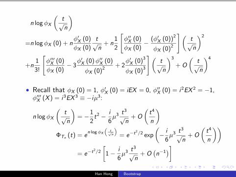
n log φX
(t√n
)=n log φX (0) + n
φ′X (0)
φX (0)
t√n
+ n1
2
[φ′′X (0)
φX (0)− (φ′X (0))2
φX (0)2
](t√n
)2
+n1
3!
[φ′′′X (0)
φX (0)− 3
φ′X (0)φ′′X (0)
φX (0)2 + 2φ′X (0)3
φX (0)3
](t√n
)3
+ O
(t√n
)4
• Recall that φX (0) = 1, φ′X (0) = iEX = 0, φ′′X (0) = i2EX 2 = −1,φ′′′X (X ) = i3EX 3 ≡ −iµ3:
n log φX
(t√n
)= −1
2t2 − i
6µ3 t3
√n
+ O
(t4
n
)ΦTn (t) = e
n log φX
(t√n
)= e−t
2/2 exp
(− i
6µ3 t3
√n
+ O
(t4
n
))= e−t
2/2
[1− i
6µ3 t3
√n
+ O(n−1)]
Han Hong Bootstrap

• Use the Inversion Formula: for φX (t) = Ee itX =∫e itx f (x) dx ,
there is f (x) = 12π
∫e−ixtφX (t) dt
• For example, the characteristic function of N (0, 1) is e−t2/2,
so e−t2/2 =
∫e itxφ (x) dx , so φ (x) = 1
2π
∫e−ixte−t
2/2dt.
• Now applying this to X = Tn:
fTn (x) =1
2π
∫e−ixtφTn (t) dt =
1
2π
∫e−ixte
n log φX
(t√n
)dt
=1
2π
∫e−ixte−
t2
2
[1− i
6µ3 t3
√n
+ O(n−1)]
dt
=1
2π
∫e−ixte−
t2
2 dt − i
6
µ3
√n
(1
2π
∫e−ixte−
t2
2 t3dt
)=
1
2π
∫e−ixte−
t2
2 dt − i
6
1
(−i)3
µ3
√n
[d
dx3
(1
2π
∫e−ixte−
t2
2 t3dt
)]+ O
(n−1)
= φ (x)− 1
6
µ3
√nφ′′′ (x) + O
(n−1)
Han Hong Bootstrap

• So
P (Tn ≤ x) =
∫ x
fTn (u) du = Φ (x)− 1
6
µ3
√nφ′′ (x) + O
(n−1)
.
• So
G (x ,F0) = −µ3
6φ′′ (x) =
µ3
6
(1− x2
)φ (x) ,
by noting that φ′ (x) = −xφ (x), and φ′′ (x) = −φ (x) + x2φ (x).Note that G (x ,F0) is an even function.
Han Hong Bootstrap

Lecture 13: Subsampling vs Bootstrap
Dimitris N. Politis, Joseph P. Romano, Michael Wolf
2011
Dimitris N. Politis, Joseph P. Romano, Michael Wolf Subsampling vs Bootstrap

Bootstrap
• Rn (xn, θ (P)) = τn
(θn − θ (P)
)• Example:
• θn = Xn, τn =√n, θ = EX = µ (P)
• θ = minXn, τn = n, θ (P) = supx : F (x) ≤ 0
• Define: Jn (P), the distribution of τn(θn − θ (P)
)under P.
For real θn,
Jn (x ,P) ≡ ProbP(τn
(θn − θ (P)
)≤ x
)• Since P is unknown, θ (P) is unknown, and Jn (x ,P) is also
unknown.
Dimitris N. Politis, Joseph P. Romano, Michael Wolf Subsampling vs Bootstrap

• The bootstrap estimate Jn (x ,P) by Jn(x , Pn), where Pn is aconsistent estimate of P in some sense.
• For example, take Pn (x) = 1n
∑ni=1 1 (Xi ≤ x)
supx
∣∣∣∣Pn (x)− P (x)
∣∣∣∣ a.s.−→ 0
• Similarly estimate (1− α)th quantile of Jn (x ,P) by Jn(x , Pn):i.e. Estimate J−1
n (x ,P) by J−1n (x , Pn).
• Usually Jn(x , Pn) can’t be explicitly calculated, use MC:
Jn(x , Pn
)≈ 1
B
B∑i=1
1(τn
(θn,i − θn
)≤ x
)for θn,i = θ
(X ∗1,i , . . . ,X
∗n,i
).
Dimitris N. Politis, Joseph P. Romano, Michael Wolf Subsampling vs Bootstrap

• When bootstrap works, for each x,
Jn(x , Pn)− Jn (x ,P)p→ 0 =⇒ J−1n (1− α, Pn)− J−1n (1− α,P)
p→ 0
• When should Bootstrap “work”? Need local uniformity inweak convergence:
• Usually Jn (x ,P) −→ J (x ,P).
• Usually Pna.s.→ P in some sense, say supx |Pn (x)−P (x) | a.s.→ 0
• Suppose for each sequence Pn s.t. Pn → P, saysupx |Pn − P| → 0, it is also true that Jn (x ,Pn) −→ J (x ,P),then it must be true that a.s. Jn(x , Pn) −→ J (x ,P)
• So it ends up having to show for Pn → P,Jn (x ,Pn)→ J (x ,P), use triangular array formulation.
Dimitris N. Politis, Joseph P. Romano, Michael Wolf Subsampling vs Bootstrap

Case When Bootstrap Works
• Sample mean with finite variance.
• supx |Fn (x)− F (x) | a.s.−→ 0.
• θ(Fn) = 1n
∑ni=1 Xi
a.s.−→ θ (F ) = E (X ).
• σ2(Fn) = 1n
∑ni=1
(Xi − Xn
)2 a.s.−→ σ2 (F ) = Var(X ).
• Use Linderberg-Feller for the triangular array, applied to thedeterministic sequence of Pn such that:
1) supx |Pn (x)− Pn (x) | → 0; 2) θ (Pn)→ θ (P);
3) σ2 (Pn)→ σ2 (P),
it can be shown that√n(Xn − θ (Pn)
) d→ N(0, σ2
)under Pn.
• Since Pn satisfies 1,2,3 a.s., therefore Jn(x , Pn)a.s.−→ J (x ,P)
• So “local uniformity” of weak convergence is satisfied here.
Dimitris N. Politis, Joseph P. Romano, Michael Wolf Subsampling vs Bootstrap

Cases When Bootstrap Fails
• Order Statistics:
F ∼ U (0, θ), and X(1), . . . ,X(n) is the order statistics of thesample, so X(n) is the maximum:
P
(nθ − X(n)
θ> x
)= P
(X(n) < θ − θx
n
)= P
(Xi < θ − θx
n
)n
=
(1
θ
(θ − θx
n
))n
=(
1− x
n
)n n→∞−→ e−x
• The bootstrap version:
P
(nX(n) − X ∗(n)
X(n)= 0
)=
(1−
(1− 1
n
)n)n→∞−→
(1− e−1
)≈ 0.63
Dimitris N. Politis, Joseph P. Romano, Michael Wolf Subsampling vs Bootstrap

• Degenerate U-statistics:
Take w (x , y) = xy , θ (F ) =∫ ∫
w (x , y) dF (x) dF (y) = µ (F )2.
θn = θ(Fn
)=
1
n (n − 1)
∑∑i 6=j
XiXj
S (x) =
∫xydF (y) = xµ (F )
• If µ (F ) 6= 0 it is known that
√n(θn − θ
)d−→ N (0, 4Var (S (X ))) = N
(0, 4
(µ2EX 2 − µ4
))The bootstrap works.
Dimitris N. Politis, Joseph P. Romano, Michael Wolf Subsampling vs Bootstrap

• But if µ (F ) = 0 =⇒ θ (F ) = 0:
θ(Fn) =1
n (n − 1)
∑∑i 6=j
XiXj = X 2n −
1
n
1
n − 1
∑i
(Xi − Xn
)2= X 2
n −S2n
n
n(θ(Fn
)− θ (F )
)= nX 2
n − S2n
d−→ N(0, σ2
)− σ2
• However the bootstrap version of n[θ(F ∗n
)− θ
(Fn)]
:
n
([X ∗2n −
1
nS∗2n
]−[X 2n −
1
nS2n
])= nX ∗2n − S∗2n − nX 2
n + S2n
≈ n(X ∗2n − X 2
n
)=[√
n(X ∗n − Xn
)]2+ 2√n(X ∗n − Xn
)√nXn
d−→ N(0, σ2
)2+ 2N
(0, σ2
)√nXn
Dimitris N. Politis, Joseph P. Romano, Michael Wolf Subsampling vs Bootstrap
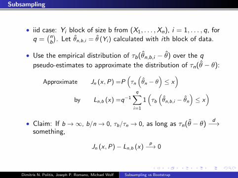
Subsampling
• iid case: Yi block of size b from (X1, . . . ,Xn), i = 1, . . . , q, forq =
(nb
). Let θn,b,i = θ (Yi ) calculated with ith block of data.
• Use the empirical distribution of τb(θn,b,i − θ) over the q
pseudo-estimates to approximate the distribution of τn(θ − θ):
Approximate Jn (x ,P) =P(τn
(θn − θ
)≤ x
)by Ln,b (x) =q−1
q∑i=1
1(τb
(θn,b,i − θn
)≤ x
)
• Claim: If b →∞, b/n→ 0, τb/τn → 0, as long as τn(θ − θ)d−→
something,
Jn (x ,P)− Ln,b (x)p−→ 0
Dimitris N. Politis, Joseph P. Romano, Michael Wolf Subsampling vs Bootstrap

Different Motivation for Subsampling vs. Bootstrap
Subsampling:
• Each subset of size b comes from the TRUE model. Sinceτn(θn − θ)
d−→ J (x ,P), so as long as b →∞:
τb(θb − θ)d−→ J (x ,P)
The distributions of τn(θn − θ) and τb(θb − θ) should be close.
• But τb(θb − θ) = τb(θb − θn) + τb(θn − θ). Since
τb
(θn − θ
)= Op
(τbτn
)= op (1)
The distributions of τb(θb − θ) and τb(θb − θn) should be close.
• The distribution of τb(θb − θn) is estimated by the empiricaldistribution over q =
(nb
)pseudo-estimates.
Dimitris N. Politis, Joseph P. Romano, Michael Wolf Subsampling vs Bootstrap
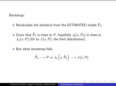
Bootstrap:
• Recalculate the statistics from the ESTIMATED model Pn.
• Given that Pn is close to P, hopefully Jn(x , Pn) is close toJn (x ,P) (Or to J (x ,P), the limit distribution).
• But when bootstrap fails
Pn −→ P ; Jn(x , Pn
)−→ J (x ,P)
Dimitris N. Politis, Joseph P. Romano, Michael Wolf Subsampling vs Bootstrap

Formal Proof of Consistency of Subsampling
• Assumptions: τn(θn − θ)d−→ J (x ,P), b →∞, b
n → 0, τbτn→ 0.
Need to show: Ln,b (x)− J (x ,P)p→ 0.
• Since τ (θn − θ)p−→ 0, it is enough to show
Un,b (x) = q−1q∑
i=1
1(τb
(θn,b,i − θ
)≤ x
)p−→ J (x ,P) .
Un,b (x) is a bth order U-statistics with kernel functionbounded by (−1, 1).
• Un,b (x)− J (x ,P) = Un,b (x)− EUn,b (x) + EUn,b (x)− J (x ,P), itis enough to show
Un,b (x)− EUn,b (x)p−→ 0 and EUn,b (x)− J (x ,P)→ 0
Dimitris N. Politis, Joseph P. Romano, Michael Wolf Subsampling vs Bootstrap
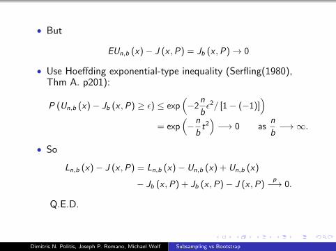
• But
EUn,b (x)− J (x ,P) = Jb (x ,P)→ 0
• Use Hoeffding exponential-type inequality (Serfling(1980),Thm A. p201):
P (Un,b (x)− Jb (x ,P) ≥ ε) ≤ exp(−2
n
bε2/ [1− (−1)]
)= exp
(−n
bt2)−→ 0 as
n
b−→∞.
• So
Ln,b (x)− J (x ,P) = Ln,b (x)− Un,b (x) + Un,b (x)
− Jb (x ,P) + Jb (x ,P)− J (x ,P)p−→ 0.
Q.E.D.
Dimitris N. Politis, Joseph P. Romano, Michael Wolf Subsampling vs Bootstrap

Time Series
• Respect the ordering of the data to preserve correlation.
θn,b,t = θb (Xt , . . . ,Xt+b−1) , q = T − b + 1.
Ln,b (x) =1
q
q∑i=1
1(τb
(θn,b,t − θn
)≤ x
)• Assumption: τn(θn − θ)
d−→ J (x ,P), b →∞, bn → 0, τb
τn→ 0,
α (m)→ 0.
• Result: Ln,b (x)− J (x ,P)p−→ 0.
• Most difficult part: To show τn(θn − θ)d−→ J (x ,P).
Dimitris N. Politis, Joseph P. Romano, Michael Wolf Subsampling vs Bootstrap

• Can treat iid data as time series, or even usingnon-overlapping blocks k =
[nb
], but using
(nb
)more efficient.
• For example, if
Un (x) = k−1k∑
j=1
1 (τb [Rn,b,j − θ (P)] ≤ x)
then
Un,b (x) = E[Un (x) |Xn
]= E [1 (τb [Rn,b,j − θ (P)] ≤ x) |Xn]
for Xn =(X(1), . . . ,X(n)
).
• Un,b (x) is better than Un (x) since Xn is sufficient statisticsfor iid data.
Dimitris N. Politis, Joseph P. Romano, Michael Wolf Subsampling vs Bootstrap

• Hypothesis Testing: Tn = τntn (X1, . . . ,Xn),
Gn (x ,P) = Probp (τn ≤ x)P∈P0−→ J (x ,P)
Gn,b (x) = q−1q∑
i=1
1 (Tn,b,i ≤ x) = q−1q∑
i=1
1 (τbtn,b,i ≤ x)
As long as b →∞, bn → 0, then under P ∈ P0:
Gn,b (x) −→ G (x ,P)
If under P ∈ P1, Tn →∞, then ∀x , Gn,b (x)→ 0.
• Key difference with confidence interval: don’t need τbτn→ 0,
because don’t need to estimate θ0 but assumed known underthe null hypothesis.
Dimitris N. Politis, Joseph P. Romano, Michael Wolf Subsampling vs Bootstrap
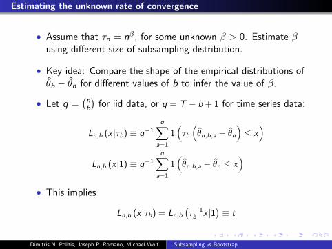
Estimating the unknown rate of convergence
• Assume that τn = nβ, for some unknown β > 0. Estimate βusing different size of subsampling distribution.
• Key idea: Compare the shape of the empirical distributions ofθb − θn for different values of b to infer the value of β.
• Let q =(nb
)for iid data, or q = T − b + 1 for time series data:
Ln,b (x |τb) ≡ q−1q∑
a=1
1(τb
(θn,b,a − θn
)≤ x
)Ln,b (x |1) ≡ q−1
q∑a=1
1(θn,b,a − θn ≤ x
)• This implies
Ln,b (x |τb) = Ln,b(τ−1b x |1
)≡ t
Dimitris N. Politis, Joseph P. Romano, Michael Wolf Subsampling vs Bootstrap

• x = L−1n,b (t|τb) = τb
(τ−1b x
)= τbL
−1n,b (t|1)
• Since Ln,b (x |τb)p−→ J (x ,P), if J (x ,P) is continuous and
increasing, it can be infered that
L−1n,b (t|τb) = J−1 (t,P) + op (1)
• Same as
τbL−1n,b (t|1) = J−1 (t,P) + op (1)
• So
bβL−1n,b (t|1) = J−1 (t,P) + op (1)
• Assuming J−1 (t,P) > 0, or t > J (0,P), take log.
Dimitris N. Politis, Joseph P. Romano, Michael Wolf Subsampling vs Bootstrap

• For different b1 and b2, then this becomes
β log b1 + log(L−1n,b1
(t|1))
= log J−1 (t,P) + op (1)
β log b2 + log(L−1n,b2
(t|1))
= log J−1 (t,P) + op (1)
• Different out the “fixed effect”
β (log b1 − log b2) = log(L−1n,b2
(t|1))− log
(L−1n,b1
(t|1))
+ op (1)
• So estimate β by
β = (log b1 − log b2)−1(
log(L−1n,b2
(t|1))− log
(L−1n,b1
(t|1)))
= β + (log b1 − log b2)−1 × op (1)
• Take b1 = nγ1 , b2 = nγ2 , (1 ≥ γ1 > γ2 > 0)
β − β = ((γ1 − γ2) log n)−1 op (1) = op(
(log n)−1)
Dimitris N. Politis, Joseph P. Romano, Michael Wolf Subsampling vs Bootstrap

• How to know t > J (0,P),
Ln,b (0|τb) = Ln,b (0|1) = J (0,P) + op (1)
So estimating J (0,P) not a problem.
• Alternatively, take t2 ∈ (0.5, 1), take t1 ∈ (0, 0.5)
bβ(L−1n,b (t2|1)− L−1n,b (t1|1)
)= J−1 (t2|P)− J−1 (t1|P) + op (1)
β log b + log(L−1n,b (t2|1)− L−1n,b (t1|1)
)= log
(J−1 (t2|P)− J−1 (t1|P)
)+ op (1)
• β = (log b1 − log b2)−1[log(L−1n,b2
(t2|1)− L−1n,b2(t1|1)
)− log
(L−1n,b1
(t2|1)− L−1n,b1(t1|1)
)]• Take b1 = nγ1 , b2 = nγ2 (1 > γ1 > γ2 > 0), β − β = op((log n)−1).
Dimitris N. Politis, Joseph P. Romano, Michael Wolf Subsampling vs Bootstrap

Two Step Subsampling
• τn = nβ
Ln,b (x |τb) = q−1q∑
a=1
1(τb
(θn,b,a − θn
)≤ x
)Can show that
supx
∣∣∣∣Ln,b (x |τb)− J (x ,P)
∣∣∣∣ p−→ 0.
• Problem: imprecise in small samples.
• In variation estimation, best choice of b gives O(n−1/3) errorrate.
• Parameter estimates, if model is true, gives O(n−1/2) errorrate.
• Bootstrap pivotal statistics, when applicable, gives even betterthan O(n−1/2) error rate.
Dimitris N. Politis, Joseph P. Romano, Michael Wolf Subsampling vs Bootstrap