nonlinear model predictive control for path following problems model... · 2019-10-16 · nonlinear...

INTERNATIONAL JOURNAL OF ROBUST AND NONLINEAR CONTROLInt. J. Robust Nonlinear Control 2015; 25:1168–1182Published online 2 January 2014 in Wiley Online Library (wileyonlinelibrary.com). DOI: 10.1002/rnc.3133

Nonlinear model predictive control for path following problems

Shuyou Yu1,2,*,† , Xiang Li2, Hong Chen1,3 and Frank Allgöwer2

1Department of Control Science and Engineering, Jilin University Changchun, China2Institute for Systems Theory and Automatic Control, University of Stuttgart Stuttgart, Germany

3State Key Laboratory of Automotive Simulation and Control, Jilin University Changchun, China

SUMMARY

This paper presents a general nonlinear model predictive control scheme for path following problems. Pathfollowing problem of nonlinear systems is transformed into a parameter-dependent regulation problem.Sufficient conditions for recursive feasibility and asymptotic convergence of the given scheme are presented.Furthermore, a polytopic linear differential inclusion-based method of choosing a suitable terminal penaltyand the corresponding terminal constraint are proposed. To illustrate the implementation of the nonlinearmodel predictive control scheme, the path following problem of a car-like mobile robot is discussed, and thecontrol performance is confirmed by simulation results. Copyright © 2014 John Wiley & Sons, Ltd.

Received 03 April 2012; Revised 06 May 2013; Accepted 22 November 2013

KEY WORDS: model predictive control; nonlinear systems; path following; feasibility and convergence

1. INTRODUCTION

Nonlinear model predictive control (NMPC), also referred to as receding horizon control or movinghorizon optimal control, has been viewed as one of standard control techniques for nonlinear sys-tems with input and state constraints [1–3]. A control sequence is obtained by solving online, at eachsampling instant, a finite horizon open-loop optimal control problem, which uses the current stateof the system as the initial state; the first control action in this sequence is applied to the system.Because it is difficult to obtain an analytical solution to constrained nonlinear optimal control prob-lem by solving the related Hamilton-Jacobi-Bellman equation, NMPC has aroused many interests inboth the academic community and the industrial society. Over the last decade, academic researchesof NMPC have made significant progresses in issues on both stability and robustness [2, 4], and itsapplications have spanned a wide range from process control [3] to aerospace [5] and to control oftransportation networks [6].

Normally, NMPC is used to deal with the so-called regulation problem, that is, to regulate thestate of a system to a fixed target state [7, 8]. However, when the target state changes, the feasibilityof the controller may be lost, and the controller fails to track the target states.

Besides the regulation problem, tracking control and path following are the other two fundamen-tal control problems. Tracking control of systems aims at tracking a given time-varying referencetrajectory. NMPC for tracking control has been discussed in [9–11] and references therein. Insteadof arbitrary but smooth trajectories, only piecewise constant references are considered. A recedinghorizon control scheme for tracking control of a nonholonomic mobile robot is developed in [12],where a control Lyapunov-based scheme is chosen to determine the terminal penalty and the termi-nal constraint of the NMPC optimization problem for the considered systems. Thus, the proposed

*Correspondence to: Shuyou Yu, Department of Control Science and Engineering, Jilin University (Nanling Campus),130025, Changchun, China.

†E-mail: [email protected]

Copyright © 2014 John Wiley & Sons, Ltd.

NONLINEAR MPC FOR PATH FOLLOWING PROBLEMS 1169

scheme is only typically fit for the given systems. The task of the path following problem is to steera system to follow a reference path. In contrast to the tracking control problem, the reference path isnot parameterized in time but in its geometrical coordinates. The papers [13, 14] propose an NMPCframework for solving the path following problem and give sufficient stability conditions. Althoughsome methods of choosing the terminal ingredients of the MPC optimization problem are proposed,they are either conservative or rely on the system property of differential flatness. The introducedNMPC framework optimizes the time evolution of the path parameter, but the initial value of thepath parameter is not considered in the online optimization problem.

This paper presents a more general NMPC scheme for the path following problem, where thetime evolution of the path parameter as well as its initial value are determined in the online opti-mization problem. Firstly, the path following problem of nonlinear systems is transformed into aparameter-dependent regulation problem. Following a discussion of recursive feasibility and asymp-totic convergence, a polytopic linear differential inclusion (PLDI)-based method is adopted tochoose the terminal penalty and the terminal constraint. To illustrate the implementation of the pro-posed NMPC scheme, the path following problem of a car-like mobile robot is discussed, and thecontrol performance is confirmed by simulation results.

The remainder of this paper is organized as follows. Section 2 sets up the path following problem.In Section 3, an NMPC scheme to the path following problem is introduced with a proof of asymp-totic convergence and recursive feasibility. A method for choosing a suitable terminal penalty andthe related terminal constraint is presented in detail. Section 4 shows the implementation of the pro-posed NMPC scheme for the path following problem of a car-like mobile robot. A short summaryis given in Section 5.

2. PATH FOLLOWING PROBLEM

For a system, an intuitive understanding of the path following problem is to approach a referencepath as close as possible. Thus, it is necessary to clarify the definition of the system and the referencepath before formulating the path following problem.A continuous time nonlinear system

Px.t/ D f .x.t/; u.t//; x.t0/ D x0; (1)

is considered, which has state and input constraints

x 2 X � Rn; u 2 U � Rm; (2)

where f .x; u/ W X � U �! Rn is continuously differentiable in x and u, U � Rm is compact, andX � Rn is connected.

The reference path is a twice continuously differentiable geometric curve, which can be definedas a set of points r parameterized by a scalar s,

P D ¹r 2 Rnj r D p.s/º; (3)

where the function p W R1 ! Rn is a twice continuously differentiable function. The scalar s isconstrained by s 2 S � R1, where S is a compact set. The time evolution of s.t/ is not necessaryto be known a priori but influenced by a virtual input v.t/ that is a DOF to choose,

Ps.t/ D v.t/; v 2 V � R1: (4)

Remark 2.1If the given path is not smooth enough, a continuously differentiable geometric curve can be usedto approximate it and can be used as the reference path.

Copyright © 2014 John Wiley & Sons, Ltd. Int. J. Robust Nonlinear Control 2015; 25:1168–1182DOI: 10.1002/rnc

1170 S. YU ET AL.

Remark 2.2If the reference path is in a subspace of Rn, that is, P0 D ¹r0 2 Rn0 j r0 D p.s/º with n0 < n, thenP can be chosen as

P D²

r 2 Rn j r D�

r00

�³

with 0 2 Rn�n0 .

The path following problem is the following:Given a geometric path P defined by (3), find admissible control values u.t/ and v.t/ such that

limt!1

xe.t/ D 0; (5)

where xe is defined by

xe.t/ WD x.t/ � p.s.t//: (6)

Two technical assumptions are made:

Assumption 1The reference path P is contained in the state constraint set of the system (1), that is, P � X .

Assumption 2There exist admissible inputs u 2 U and v 2 V , such that the dynamics of the state x.t/ 2 X andthe parameter s.t/ 2 S satisfy

Pxe.t/ D 0; (7)

if xe.t/ D 0.

Remark 2.3Assumption 1 ensures the existence of at least one x 2 X matching each point on the reference pathP . Together, Assumption 1 and Assumption 2 guarantee that the system (1) can indeed follow thegiven path (3).

The dynamics of the error system (6) is

Pxe D Px � Œp.s/�0 D f .x; u/ �@p@sv: (8)

It shows that the error dynamics are continuously differentiable in x, u, s, and v because f .�; �/ iscontinuously differentiable and p.�/ is twice continuously differentiable. The dynamics of the errorsystem (6) is a function of xe , u, s, and v, because x D xe C p.s/ and

Pxe D f .xe C p.s/;u/ �@p@sv: (9)

Assumption 3There exist a continuously differentiable function g.�; �/ and a control input ue such that

Pxe WD g.xe;ue/; (10)

where the function g is parameter-dependent in s and v, the control input ue 2 Rm is an implicitfunction of u, s, and v.

Because the control input of the error system ue is an implicit function of u, s, xe and v, abuse ofnotation, denote h.xe;u; s; v// as the expression of the implicit function. Then, Equation (10) can berewritten as xe.t/ D g.xe; h.xe;u; s; v//, which confirms that the function g is parameter-dependentin s and v.



In terms of Assumption 1 and Assumption 2, .0; 0/ is the equilibrium of the error dynamics (10),that is, g.0; 0/ D 0. The term ue has to satisfy the following assumption:

Assumption 4There exist a compact set Ue such that ue 2 Ue and 0 2 Ue .

Remark 2.4Assumption 4 is only used to find a terminal set that will be introduced in the next section.

Remark 2.5 (A way to find the function g.xe; ue/)Suppose that there exists continuously differentiable functions h1.xe; s; v/ and h2.xe; s; u; v/such that

f .xe C p.s/; u/ �@p@sv D h1.xe; s; v/C h2.xe; s;u; v/;

and there exist s 2 S, v 2 V , and u 2 U such that h1.xe; s; v/ D 0 and h2.xe; s;u; v/ D 0, whilexe D 0, we can choose ue WD h2.xe; s;u; v/, which results in g.xe;ue/ D h1.xe; s; v/C ue .

Because of Assumption 2, we know that while xe.t/ D 0, there exist admissible inputs u 2 U andv 2 V , such that the dynamics of the state x.t/ 2 X and the parameter s.t/ 2 S satisfy Pxe.t/ D 0.That is,

0 Dg.0; ue/

Df .p.s/; u/ �@p@sv:

Thus, one option is to choose h1.xe; s; v/ � 0 and h2.xe; s; u; v/ D f .xe C p.s/;u/ � @p@sv.

Therefore, the existence of the functions h1 and h2 is guaranteed.

Remark 2.6By choosing g.�; �/ and ue such that Assumption 3 is satisfied, we transform the path followingproblem into a parameter-dependent regulation problem, where .0; 0/ is the target state, s and v arethe time-varying parameters.

Remark 2.7Fundamental control problems can be roughly classified into three groups, which are point stabi-lization, tracking, and path following. Point stabilization and trajectory tracking problems can beseen as two special cases of the path following problem. While s.t/ � c for all t , where c is a con-stant, the path following problem reduces to a point stabilization (regulation) problem; while s.t/ isexactly predefined, the path following problem is equal to a trajectory tracking problem. Comparingwith the trajectory tracking problem, the path following problem has one additional DOF, which isto regulate the dynamics of s.

3. NONLINEAR MODEL PREDICTIVE CONTROL FOR PATH FOLLOWING PROBLEMS

In this section, we will discuss an NMPC scheme for the path following problem. After formulatingthe online optimization problem, a proof of recursive feasibility and asymptotic convergence of theintroduced NMPC scheme is presented. Furthermore, a PLDI-based algorithm is proposed to choosea suitable terminal penalty and the related terminal constraint.

3.1. Optimization problem and algorithm

In order to formulate the path following problem within the NMPC framework, we consider thefollowing online optimization problem at time instant t :


1172 S. YU ET AL.

Problem 1

minimizeu.�;x.t//;v.�;x.t//;s.t;x.t//

J.x.t// (11a)

subject to

Px.�; x.t// D f .x.�; x.t//; u.�; x.t///; (11b)

Ps.�; x.t// D v.�; x.t//; x.t; x.t// D x.t/; (11c)

xe.�; x.t// D x.�; x.t// � p.s.�; x.t///; (11d)

u.�; x.t// 2 U ; x.�; x.t// 2 X ; (11e)

v.�; x.t// 2 V; s.�; x.t// 2 S; (11f)

xe.t C Tp; x.t// 2 �; (11g)

with

J .x.t// D E.xe.t C Tp; x.t///CZ tCTp

t

F.xe.�; x.t//; ue.�; x.t///d�; (12)

where J.x.t// is the cost functional, and Tp is the prediction horizon. The term ue.�; x.t// denotesthe predicted input function of the error system related to x.t/, and xe.�; x.t// represents the pre-dicted state trajectory of the error system under the control ue.�; x.t//. The termsE.xe.tCTp; x.t///and xe.tCTp; x.t// 2 � are the terminal penalty and the terminal constraint, respectively, which areused to guarantee recursive feasibility and achieve asymptotic convergence to the given path. Theterm F.�; �/ is the stage cost function, which specifies the desired control performance and satisfiesthe following condition.

Assumption 5F.�; �/ W X �U ! R1 is continuous, and F.0; 0/ D 0 and F.x;u/ > 0 for all .x;u/ 2 X �U n¹0; 0º.

For clarity, u.�; x.t// denotes the predicted input function related to the measured state x.t/ attime instant t , and x.�; x.t// represents the predicted state trajectory starting from x.t/ under thecontrol u.�; x.t//, for all � 2 Œt; t CTp�. The notations v.�; x.t//, s.�; x.t//, and xe.�; x.t// refer tothe predicted values of v, s, and xe at time � related to x.t/, respectively.

Remark 3.1The cost functional J and the terminal constraint xe.t C Tp; x.t// 2 � do not depend explicitly onthe parameter s or v, which is consistent with the fact that s and v only describe a virtual referencemotion.

Suppose the sampling time is ı, the proposed NMPC control law is formally described by thefollowing algorithm.

Algorithm 1Step 1: Measure system state x.t/ at time t ,Step 2: Solve Problem 1 and obtain a feasible (suboptimal) solution s0.t; x.t//, u0.�; x.t// andv0.�; x.t// for � 2 Œt; t C Tp�,Step 3: Take the input value u0.�; x.t//, � 2 Œt; t C ı�, as the current input for the system,Step 4: Take the input value v0.�; x.t// and the initial state s0.t; x.t// to update the pathparameter s.�; x.t// for � 2 Œt; t C ı�,Step 5: Set t WD t C ı, go to Step 1.

Remark 3.2The initial state of Ps.t/ D v.t/ is chosen as a determined variable in Problem 1, that is, the referencemotion s.t/ is renewed entirely at each time instant. Thus, it provides an extra DOF of optimizationproblem.



Remark 3.3Because Problem 1 is a nonlinear and nonconvex optimization problem, in general, it is impossibleto obtain the exact globally optimal solution even if there exists a globally optimal solution.

3.2. Feasibility and stability

As important issues of ensuring feasibility and convergence of the NMPC scheme, the terminalpenalty E.xe/, the terminal set �, and the corresponding fictitious terminal control law �.xe/ arerequired to satisfy the following conditions:

B0. � � X ,B1. �.0/ D 0, and �.xe/ 2 Ue for all xe 2 �,B2. E.0/ D 0, and E.xe/ satisfies

@E.xe/@xe

g.xe; �.xe//C F.xe; �.xe// 6 0; (13)

for all xe 2 �.

As a neighborhood of the error state xe D 0,

� WD ¹xe 2 Rn j E.xe/ 6 ˛º; (14)

with ˛ > 0.Clearly, the terminal set � has the following additional properties:

1. The point 0 2 Rn is contained in the interior of � because of the positive definiteness ofE.xe/.

2. � is closed and connected because of the continuity of E.xe/.3. � is robustly invariant for the nonlinear system (10) controlled by ue D �.xe/, for all s.�/ 2 S

and v.�/ 2 V because of (13).

Assumption 6For the error system (10), there exist a locally asymptotically stabilizing controller �.xe/, a termi-nal set � � X , and a continuously differentiable, positive semi-definite function E.xe/ such thatconditions B0–B2 are satisfied for all xe 2 �.

Assumption 7There exist s 2 S and v 2 V such that x 2 X and u 2 U , while xe 2 � and ue 2 Ue .

Now, we are ready to show the recursive feasibility of the considered optimization problem and theasymptotic convergence of the path following problem.

Theorem 1Suppose that

(a) Assumptions 1–7 are satisfied,(b) at the initial time instant, Problem 1 has a feasible solution,

then,

1. Problem 1 is feasible for all time instants,2. the system state x.t/ follows the predefined geometric path P asymptotically, that is,

limt!1 xe.t/ D 0:

ProofAssume that Problem 1 has a feasible solution at time instant t , which is�u0.�; x.t//; v0.�; x.t//; s0.t; x.t//

�for � 2 Œt; t C Tp�. The corresponding input and the state of

the error system (10) are u0e.�; x.t// and x0e.�; x.t//, respectively.


1174 S. YU ET AL.

1. The input u0.�; x.t// is implemented, and the related dynamic of the system (1) is x0.�; x.t//,for all � 2 Œt; t C ı�. The solution s0.�; x.t// and v0.�; x.t//, � 2 Œt; t C Tp� are used toobtain the evolution of the system (4). Because neither model-plant mismatches nor externaldisturbances are present, x.t C ı/ D x0.t C ı; x.t//. Thus, the remaining piece of the inputsu0.�; x.t// and v0.�; x.t//, � 2 Œt C ı; t C Tp� satisfy the constraints of Problem 1. Denotex0.tCTp/ WD x0.tCTp; x.t//. Because x0e.tCTp; x.t// 2 �, it follows from Assumptions 6and 7 that �.�/ renders� invariant, and there exist s.�; x0.tCTp// 2 S and v.�; x0.tCTp// 2V such that x.�; x0.t C Tp// 2 X and u.�; x0.t C Tp// 2 U , for all � 2 Œt C Tp; t C Tp C ı�.The dynamics of the error system (10) under the terminal control law �.�/ is xe.�; x0.t CTp// for all � � t C Tp . Therefore, a feasible solution to Problem 1 at time instant t C ı is.u.�; x.t C ı//; v.�; x.t C ı//; s.t C ı; x.t C ı/// where s.tC ı; x.tC ı// WD s0.tC ı; x.t//,and

u.�; x.t C ı// WD²

u0.�; x.t// � 2 Œt C ı; t C Tp/;

u.�; x0.t C Tp// � 2 Œt C Tp; t C Tp C ı�;

v.�; x.t C ı// WD²v0.�; x.t// � 2 Œt C ı; t C Tp/;

v.�; x0.t C Tp// � 2 Œt C Tp; t C Tp C ı�:

2. Let us define a Lyapunov-like function candidate as

V.x.t// WD J.x.t//; (15)

for fixed u0.�; x.t//, v0.�; x.t//, and s0.t; x.t//, with � 2 Œt; tCTp�. Note that 0 6 V.x.t// <C1, which follows directly from the definition of V.�/ and V.x.t// D 0, while x.t/ Dp.s.t//.At time instant t , the cost functional is

V.x.t// D E�x0e.t C Tp; x.t//

�C

Z tCTp

t

F�x0e.�; x.t//; u

0e.�; x.t//

�d�: (16)

Note that V.x/ is not unique because only a feasible solution is considered. Considering thefeasible solution at time instant t C ı for Problem 1, and recalling �.�/, which renders �invariant, we have

J.x.t C ı// D E�xe.t C ı C Tp; x0.t C Tp//

�

C

Z tCTp

tCı

F�x0e.�; x.t//; u

0e.�; x.t//

�d�

C

Z tCTpCı

tCTp

F�xe.�; x0.t C Tp//; �.xe.�; x0.t C Tp//

�d�:

(17)

Because the ‘possible" solution is better than the feasible solution, otherwise, we can usedirectly the feasible solution, we have V.x.t C ı// 6 J.x.t C ı//. Thus,

V.x.t C ı// � V.x.t// 6 J.x.t C ı// � V.x.t//

D �

Z tCı

t

F�x0e.�; x.t//; u

0e.�; x.t//

�d�

C

Z tCTpCı

tCTp


�d�

CE�xe.t C ı C Tp; x0.t C Tp//

��E

�x0e.t C Tp; x.t//

�:

From the integration of inequality (13), the aforementioned inequality

E�xe.t C ı C Tp; x0.t C Tp//

��E

�x0e.t C Tp; x.t//

�

6 �Z tCTpCı

tCTp


�d�



results in

V.x.t C ı// � V.x.t// 6 �Z tCı

t

F.x0e.�; x.t//; u0e.�; x.t///d�:

Clearly, V.x.t// is a monotonically decreasing function and has zero as its low bound. Thestate of the error system (10) will converge to zero as time increases [7]. Accordingly, the stateof the system (1) will finally follow the reference path (3), that is, limt!1 xe.t/ D 0.

�

Remark 3.4The aforementioned proof shows that applying feasible solution to optimization problem at eachtime instant is sufficient to guarantee both recursive feasibility and asymptotic convergence. This isone of the main advantages of the proposed NMPC scheme.

Remark 3.5Because limt!1 xe.t/ D 0 rather than xe � 0, while t !1; see Theorem 1, the reference path isnot necessary an admissible trajectory of the systems.

3.3. Terminal set with a static terminal control law

To choose a suitable pair of terminal penalty and terminal constraint that satisfies all the assumptionsand conditions earlier, we will propose a PLDI-based method. The calculated terminal control law isrobust with respect to the parameters v and s, and the terminal set is a corresponding robust invariantset.

Firstly, we discuss how to guarantee the satisfaction of inequality (13), while a quadratic stagecost F.xe;ue/ WD xTe Qxe C uTe Rue is considered.

Because xe D 0 is an equilibrium of the error system (10), there exists a set †0 such that, for allxe 2 Xe and ue 2 Ue ,

g.xe;ue/ 2 †0

�xeue

�;

where Xe � X is a compact set, †0 � Rn�.nCm/ is a parameterized differential inclusion of thenonlinear system (10) with respect to the parameters s and v.

Because s 2 S and v 2 V , and S and V are compact sets, †0 can be bounded by a PLDI †

† WD Co®�A1x B1u

�; : : : ;

�ANx BNu

�¯; (18)

that is, †0 � †. The term N is the number of vertex matrices,�Aix Biu

�is the vertex matrix of

the set †, where i 2 Œ1; N �, Aix 2 Rn�n, and Biu 2 Rn�m.Note that, since the error system (10) is continuously differentiable, the set † can be obtained by

choosing [email protected] ;ue/@xe

@g.xe ;ue/@ue

i2 †;

for all xe 2 Xe , ue 2 Ue , s 2 S, and v 2 V .Based on the PLDI in (18), a sufficient condition that guarantees the satisfaction of Equation (13)

is proposed, which is given in terms of linear matrix inequalities (LMIs).

Theorem 2Let Q 2 Rn�n and R 2 Rm�m be given. Suppose that the PLDI of the system (10) is described by(18) and suppose that there exist a matrix X > 0 with X 2 Rn�n and a matrix Y 2 Rm�n such that2

4AixX C BiuY C .AixX C BiuY /T X Y T

X �Q�1 0

Y 0 �R�1

35 6 0; (19)

for all i 2 Œ1; N �. Then, for the system (10), inequality (13) is satisfied, where E.xe/ WD xTe P xe ,P D X�1, and �.xe/ D YX�1xe .


1176 S. YU ET AL.

ProofFor simplicity, denote K WD YX�1. By substituting P D X�1 and Y D KX in (19) and byperforming a congruence transformation with the matrix ¹X�1; I; I º, we obtain

24A

Ti;clP C PAi;cl I KT

I �Q�1 0

K 0 �R�1

35 6 0;

where Ai;cl WD Aix C BiuK, I is the compatible identity matrix. It follows from the Schurcomplement that the matrix inequality (19) is sufficient to guarantee

Œg.xe; Kxe/�TP C Pg.xe; Kxe/CQCKTRK 6 0: (20)

We choose E.xe/ D xeTP xe as a Lyapunov function candidate, and ue D Kxe , the time derivative

of E.xe/ along the trajectory of (10) is given as follows:

dE.xe.t//dt

D Pxe.t/TP xe.t/C xe.t/TP Pxe.t/

D xe.t/T®Œg.xe; Kxe/�TP C Pg.xe; Kxe/

¯xe.t/:

Because of (20), we have

dE.xe.t//dt

6 �xe.t/TQxe.t/ � xe.t/TKTRKxe.t/:

Thus, the inequality (13) holds, and �.xe/ is the associated terminal control law. �Theorem 2 shows that �.xe/ and E.xe/ as given earlier can serve as a terminal control law and a

terminal penalty, respectively, for the proposed NMPC scheme.From the aforementioned discussion, an algorithm is proposed to determine a terminal penalty

matrix P and a terminal set � offline such that inequality (13) holds true, and the input constraintsue 2 Ue are satisfied.

Algorithm 2Initialization: The matrices Q 2 Rn�n and R 2 Rm�m be given.Step 1: Solve LMI (19) to obtain a locally stabilizing linear state feedback law �.xe/ and apositive definite matrix P ,Step 2: Find the largest positive ˛ such that � 2 Xe and �.xe/ 2 Ue for all xe 2 �.

Remark 3.6An algorithm for simultaneous satisfaction of (19) and the input and state constraints are discussedin [15]. As an alternative, similar algorithms that satisfy (19) and the constraints separately areproposed in [7, 16].

Remark 3.7Because the system (1) can follow the reference path if xe D 0 because of Assumptions 1 and 2, thereference path can be chosen as the terminal set, that is, � WD ¹0º, while LMI (19) has no feasiblesolution. To satisfy the Assumption 6, the corresponding terminal penalty and the terminal controllaw can be E.�/ WD 0 and �.�/ WD 0, respectively.

4. PATH FOLLOWING CONTROL OF A CAR-LIKE MOBILE ROBOT

To illustrate the implementation of the proposed NMPC scheme, the path following problem of acar-like mobile robot is considered in this section.



Figure 1. Path following problem of a car-like mobile robot.

4.1. Problem formulation

A car-like mobile robot is a kind of nonholonomic robot, which is not able to move in the directionparallel to the wheels’ axes. With definition of a world coordinate system ¹W º composed of axesXw and Yw shown in Figure 1, the kinematics model of the car-like mobile robot is described by2

4 PxRPyRPR

35 D

24 vR cos˛RvR sin˛R!v

35 ; (21)

where xR and yR denote the position of the robot center of mass with respect to ¹W º, vR is themagnitude of the robot translational velocity, ˛R denotes the robot moving direction, and !v is theangular velocity of ˛R.

To depict the path following problem of the car-like mobile robot, Figure 1 shows also a mobilerobot coordinate system ¹MRº with axes Xm and Ym, which is located at the mass of center MR

of the robot, and a path coordinate system ¹MQº composed of axes Xt and Yn, which plays a roleof the body-axis of a Virtual Vehicle to be followed. The Virtual Vehicle moves along the referencepath P and its position MQ is determined by the curvilinear abscissa s.t/. Let vectors PR and PQdescribe the positions of MR and MQ in ¹W º, wRm and wRp present the transformation matricesfrom ¹MRº to ¹W º and from ¹MQº to ¹W º, respectively, the position relationship can be deduced:

PR D PQ C wRp

�xeye

; (22)

where xe and ye denote the robot position MR with respect to ¹MQº.Computing the time derivatives of (22) and some calculation leads to the error kinematics model

of the path following problem

Pxe D

24 .yec.s/ � 1/v C vR cos˛e�xec.s/v C vR sin˛e

!v � c.s/v

35 (23)

where the error vector with respect to ¹MQº is xe WD Œxe; ye; ˛e�T , ˛e D ˛R � �p presents the

angular error between the robot moving direction ˛R and the path tangent direction �p . The valueof s is the arc length measured along the path from its origin to the point p.s/, and c.s/ denotes thepath curvature at point MQ.

Based on the error kinematics model (23), the path following problem of a car-like mobile robotcan be formulated as follows:

Given a geometric path P defined by (3), find suitable control laws of v and !v to drive the errorsxe , ye , and ˛e to zero, while vR is assigned with a nonzero magnitude value of the desired velocity.

It is noticed in model (23) that the errors can stay on the equilibrium .xe D 0/ when vapproaches vR.


1178 S. YU ET AL.

4.2. Simulation setup

Considering the geometrical symmetry and sharp changes in curvature, an eight-shaped curve isadopted as the reference path,

xP D 1:8sin. /

yP D 1:2sin.2 /;(24)

where is a path parameter and determines the path point ŒxP ; yP � with respect to the worldcoordinate system. It has bounded curvature value of �3:28 6 c.s/ 6 3:28. The changing velocityof s is bounded by 0 6 v 6 1:2 m/s.

The car-like robot is required to move with a constant velocity vR D 0:7m/s. The angular velocityis bounded by �2:5 6 !v 6 2:5 rad/s.

By choosing different Lyapunov functions of the positional and angular errors, many nonlin-ear control approaches have been presented [17–21]. However, most of them rarely take the robotconstraints into account, which are crucial for robot performance, and may even destroy the conver-gence in some cases [22, 23]. In contrast to them, the proposed NMPC scheme takes the constraintsinto account and achieves the expected performance.

4.3. Nonlinear model predictive control law design

To implement the proposed NMPC scheme for the path following problem of a car-like mobilerobot, the error kinematics model (23) needs to be transformed into the form satisfying g.0; 0/ D 0.Denoting states xe D Œxe1; xe2; xe3�T D Œxe; ye; ˛e�T and defining inputs ue WD Œue1; ue2�T with�

ue1ue2

�D

��v C vR cos xe3!v � c.s/v

�; (25)

the model (23) is rewritten as a candidate of the required error model, where

Pxe D

24 xe2c.s/v C ue1�xe1c.s/v C vR sin xe3

ue2

35 : (26)

A quadratic function is selected as the stage cost function,

F.xe;ue/ D xTe Qxe C uTe Rue: (27)

The weight matrices are chosen withQ D 0:5I3 and R D 0:5I2, where Ij denotes the unit diagonalmatrix of dimension j . The prediction horizon is 10, and the sampling time of ı is 0:02 sec.

To choose the terminal penalty and the terminal constraint, we use the scheme presented inSection 3.3. The terminal penalty is

E.xe.t C Tp// D xe.t C Tp/TP xe.t C Tp/: (28)

The terminal constraint is chosen as a sublevel set of the terminal penalty, that is,E.xe.tCTp// 6 ˛.The value of P and ˛ comes from Algorithm 2, where the PLDI of the error kinematics model

(23) is required. According to the following partial derivative,

�@g

@xe1

@g

@xe2

@g

@xe3

@g

@ue1

@g

@ue2

�D

24 0 c.s/v 0 1 0

�c.s/v 0 vR cos xe3 0 0

0 0 0 0 1

35 ; (29)

the vertex matrix of the PLDI can be obtained based on the boundary values of v and c.s/, whilethey are all bounded variables defined by the reference path.

Here, by defining 0:05 6 vR cos˛e 6 0:7 and by taking the limits of the car-like robot and theeight-shaped reference path into account, we obtain the following vertex matrices of the PLDI basedon (29),



�A1 B1

�D

24 0 3:28 0 1 0

�3:28 0 0:7 0 0

0 0 0 0 1

35 ;

�A2 B2

�D

24 0 �3:28 0 1 0

3:28 0 0:7 0 0

0 0 0 0 1

35 ;

�A3 B3

�D

24 0 3:28 0 1 0

�3:28 0 0:05 0 0

0 0 0 0 1

35 ;

�A4 B4

�D

24 0 �3:28 0 1 0

3:28 0 0:05 0 0

0 0 0 0 1

35 :

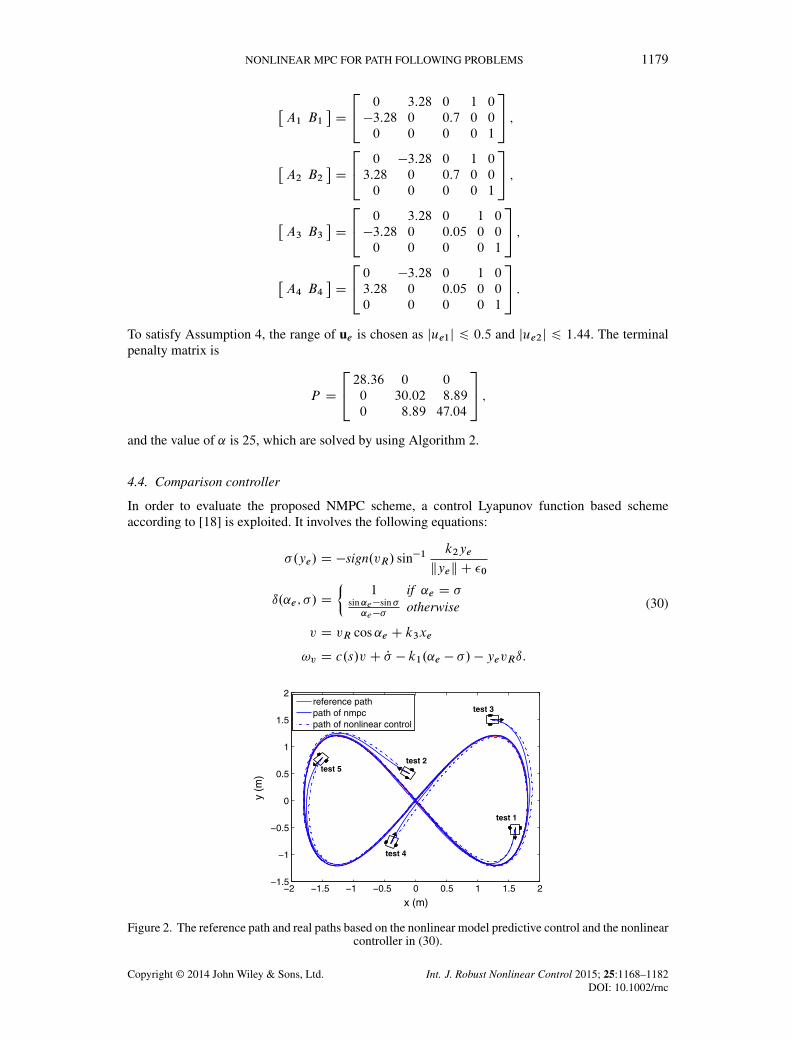
To satisfy Assumption 4, the range of ue is chosen as jue1j 6 0:5 and jue2j 6 1:44. The terminalpenalty matrix is

P D

24 28:36 0 0

0 30:02 8:89

0 8:89 47:04

35 ;

and the value of ˛ is 25, which are solved by using Algorithm 2.

4.4. Comparison controller

In order to evaluate the proposed NMPC scheme, a control Lyapunov function based schemeaccording to [18] is exploited. It involves the following equations:

�.ye/ D �sign.vR/ sin�1k2ye

kyek C �0

ı.˛e; �/ D

²1 if ˛e D �

sin˛e�sin�˛e��

otherwise

v D vR cos˛e C k3xe

!v D c.s/v C P� � k1.˛e � �/ � yevRı:

(30)

Figure 2. The reference path and real paths based on the nonlinear model predictive control and the nonlinearcontroller in (30).


1180 S. YU ET AL.

For some k1; k3 > 0, 0 < k2 6 1, and �0 > 0, this controller guarantees global stability, whichis proven by choosing the Lyapunov function V D 1

2x2e C

12y2e C

12.˛e � �/

2. Here, the controlparameters are chosen as k1 D 15, k2 D 0:8, k3 D 10, and �0 D 1.

4.5. Simulation results

In the simulation, the robot was started from five different initial positions with different headingdirections. As Figure 2 shows, both controllers are capable of driving the robot to follow the ref-erence path, but the path based on the NMPC scheme converges faster. Figure 3 shows the values

Figure 3. The velocities v and the angular velocities !v from the nonlinear model predictive control and thenonlinear controller in (30), which are shown in a solid line and a dashed line, respectively, t 2 Œ0; 20�.

0 0.2 0.4−4

−3.5

−3

−2.5

−2

−1.5

−1

−0.5

0

0.5

1test 1

time (s)

Wv

(m/s

)

0 0.2 0.4−4

−3.5

−3

−2.5

−2

−1.5

−1

−0.5

0

0.5

1test 2

time (s)0 0.2 0.4

−4

−3.5

−3

−2.5

−2

−1.5

−1

−0.5

0

0.5

1test 3

time (s)0 0.2 0.4

−4

−3.5

−3

−2.5

−2

−1.5

−1

−0.5

0

0.5

1test 4

time (s)0 0.2 0.4

0

0.5

1

1.5

2

2.5

3

3.5

4

4.5

5test 5

time (s)

Figure 4. The angular velocities !v from the nonlinear model predictive control and the nonlinear controllerin (30), which are shown in a solid line and a dashed line, respectively, t 2 Œ0; 0:4�.



of !v and v from the two controllers. It is clear that the difference only appear at the initial periodof the simulation, and it follows the reference path once the robot steps on the reference path. Thetwo controllers have similar control performance when the error Pxe is small, because the nonlinearcontroller (30) has similar form of the designed ue; see (25). Although the values of v generatedby the nonlinear controller located inside the boundary Œ0; 1:2� during the initial period, Figure 4shows that the initial errors result in big values of the angular velocity !v generated by the nonlin-ear controller. However, the NMPC takes the constraints into account, whose outputs are all insidethe boundary values.

5. CONCLUSIONS

This paper presented a general NMPC scheme for the path following problem, where the time evo-lution of the path parameter and its initial value are all determined online. Not only the asymptoticconvergence and the recursive feasibility of the proposed NMPC scheme, but also a PLDI-basedmethod to choose the terminal penalty and the terminal constraint were shown. To illustrate theimplementation of the proposed NMPC scheme, the path following problem of a car-like mobilerobot was discussed in detail. Compared with a well-known nonlinear control algorithm, theadvantage of the proposed NMPC scheme is shown in the simulation results.

ACKNOWLEDGEMENTS

Shuyou Yu and Hong Chen gratefully acknowledge the support by the 973 Program under grant no.2012CB821202 and by the Program for Changjiang Scholars and Innovative Research Team in Universityunder grant no. IRT1017. Shuyou Yu, Xiang Li and Frank Allgöwer would also like to thank the GermanResearch Foundation (DFG) for their financial support of the project AL 316=6 � 1.

REFERENCES

1. Findeisen R, Imsland L, Allgöwer F. State and output feedback nonlinear model predictive control: an overview.European Journal of Control 2003; 9(2-3):179–195.

2. Mayne DQ, Rawlings JB, Rao CV, Scokaert POM. Constrained model predictive control: stability and optimality.Automatica 2000; 36(6):789–814.

3. Qin SJ, Badgwell TA. A survey of industrial model predictive control technology. Control Engineering Practice2003; 11(7):733–764.

4. Rawlings JB, Mayne DQ. Model Predictive Control: Theory and Design. Nob Hill Publishing: Madison, Wisconsin,2009.

5. Jadbabaie A, Hauser J. Control of a thrust-vectored flying wing: a receding horizon–LPV approach. InternationalJournal of Robust Nonlinear Control 2002; 12:869–896.

6. Negenborn RR, Schutter BD, Hellendoorn H. Multi-agent model predictive control for transportation networks: serialversus parallel schemes. The 12th IFAC Symposium on Information Control Problems: IFAC, Saint-Etienne, France,2006; 339–344.

7. Chen H, Allgöwer F. A quasi-infinite horizon nonlinear model predictive control scheme with guaranteed stability.Automatica 1998; 34(10):1205–1217.

8. Magni L, Nicolao GD, Scattolini R. A stabilizing model-based predictive control algorithm for nonlinear systems.Automatica 2001; 37(9):1351–1362.

9. Chisci L, Zappa G. Dual mode predictive tracking of piecewise constant references for constrianed linear systems.International Journal of Control 2003; 76(1):61–72.

10. Ferramosca A, Limon D, Alvarado I, Alamo T, Camacho EF. MPC for tracking of constrained nonlinear systems.Proceedings of the 48th IEEE Conference Decision Control and 28th Chinese Control Conference, Shanghai, P.R.China, 2009; 7978–7983.

11. Limon D, Alvarado I, Camacho EF. MPC for tracking piecewise constant reference for constrained linear systems.Automatica 2008; 44:2382–2387.

12. Gu D, Hu HS. Receding horizon tracking control of wheel mobile robots. IEEE Transactions on Control SystemsTechnology 2006; 14(4):743–749.

13. Faulwasser T, Findeisen R. Constrained output path-following for nonlinear systems using predictive control.Proceedings of 8th IFAC Symposium on Nonlinear Control Systems (NOLCOS), Bologna, Italy, 2010; 753–758.

14. Faulwasser T, Kern B, Findeisen R. Model predictive path-following for constrained nonlinear systems. Proceedingsof the 48th IEEE Conference on Decision and Control Held Jointly with the 2009 28th Chinese Control ConferenceCDC/CCC 2009, Shanghai, China, 2009; 8642–8647.


1182 S. YU ET AL.

15. Chen WH, O’Reilly J, Ballance DJ. On the terminal region of model predictive control for nonlinear systems withinput/state constraints. International Journal of Adaptive Control and Signal Processing 2003; 17(3):195–207.

16. Michalska H, Mayne DQ. Robust receding horizon control of constrained nonlinear systems. IEEE Transactions onAutomatic Control 1993; 38(11):1623–1633.

17. Egerstedt M, Hu X, Stotsky A. Control of mobile platforms using a virtual vehicle approach. IEEE Transactions onAutomatic Control 2001; 46(11):1777–1782.

18. Ghabcheloo R, Pascoal A, Silvestre C, Kaminer I. Coordinated path following control of multiple wheeled robotswith directed communication links. Proceedings of the 44th IEEE Conference on Decision and Control, Seville,Spain, 2005; 7084–7089.

19. Li X, Zell A. Motion control of an omnidirectional mobile robot. Proceedings of the 4th International Conference onInformatics in Control, Automation and Robotics, Angers, France, 2007; 181–193.

20. Macek K, Petrovic I, Siegwart R. A control method for stable and smooth path following of mobile robots.Proceedings of the 2nd European Conference on Mobile Robots (ECMR), Ancona, Italy, 2005; 128–133.

21. Soetanto D, Lapierre L, Pascoal A. Adaptive, non-singular path-following control of dynamic wheeled robots.Proceedings of International Conference on Advanced Robotics, Coimbra, Portugal, 2003; 1387–1392.

22. Indiveri G, Paulus J, Plöger PG. Motion control of swedish wheeled mobile robots in the presence of actuatorsaturation. Proceedings of the 10th Annual Robocup International Symposium, Breme, Germany, 2006; 35–46.

23. Conceição AS, Moreira AP, Costa Pj. Trajectory tracking for omni-directional mobile robots based on restrictionsof the motor’s velocities. Proceedings of the 8th International IFAC Symposium on Robot Control, Santa CristinaConvent, Italy, 2006; 121–125.


nonlinear model predictive control for path following problems model... · 2019-10-16 · nonlinear...

Documents