nonlinear dynamic analysis efficiency by using a … · with that obtained by abaqus. ... nonlinear...

Abstract—A graphics processing unit (GPU) parallelization

approach was implemented to improve the efficiency of nonlinear dynamic analysis. The GPU parallelization approach speeded up the computation of implicit time integration and reduced total calculation time. In addition, a parallel equations solver is introduced to solve the equation system. Numerical examples of reinforced concrete (RC) frames were used to investigate the parallel computing speedup of the GPU parallelization approach. An implementation of these RC frame models for fiber beam-column elements was presented. The parallel finite element program is developed to provide parallel execution on personal computer (PC) with different CUDA-capable GPUs. The different number of degrees of freedom from low to high was adopted in the numerical examples. Detailed tests on accuracy, runtime, and speedup are conducted on different GPUs. The nonlinear dynamic response using the GPU parallelization program was in good agreement with that obtained by ABAQUS. Numerical studies indicate that compared with original sequential approach, the GPU parallelization program achieves a 22 times speedups of the solving equation system and improves the overall efficiency of time integration by up to 94%.

Index Terms—Equations Solver, Finite Element Method, GPU Parallelization, Nonlinear Dynamic Analysis

I. INTRODUCTION

he refined structure model is computationally intensive, especially for large-scale three dimensional (3D) models,

this makes the process of nonlinear finite element dynamic structural analysis much time consuming. Many modern parallel algorithms and strategies have been proposed to reduce the computing time so that engineers could spend a reasonable time to conduct the nonlinear dynamic structural analysis. Parallel algorithms applied to finite element structural analysis focusing rigorously on parallel equations solver method and domain decomposition method [1]. Parallel equations solver method generally employed the direct methods or iterative methods to solve linear system of equations, such as Jacobi, Gauss-Seidel, Conjugate Gradients

Manuscript received April 11, 2015; revised July 20, 2015. This work was

supported in part by the Major International (Sino-US) Joint Research Project of the National Natural Science Foundation of China (No. 51261120374) and the National Natural Science Foundation of China (Nos. 51278155 and 51378007).

Hong-yu Li, Jun Teng and Zuo-hua Li are with the School of Civil and Environment Engineering, Shenzhen Graduate School, Harbin Institute of Technology, Shenzhen, China (phone: 086-755-26033806; fax: 086-755-26033509; email: [email protected], [email protected], [email protected]). Jun Teng is the corresponding author.

Lu Zhang is with the Department of Civil and Materials Engineering, University of Illinois at Chicago, Chicago, IL 60607, USA (email: [email protected]).

(CG), etc. Using decomposition method, the structure was partitioned into several substructures implemented on computers or computer clusters utilizing different application programming interfaces (APIs), such as Open Multi-Processing (OpenMP) and Message Passing Interface (MPI) [2]. Although many popular parallel equations solvers and domain decomposition methods have been applied to dynamic structural analysis, some challenges still remain. The more complicated analysis tasks would be carried out, the higher resolution meshes and smaller time increments are required. Directly, more time are needed in those processes. This is still a bottleneck of parallel efficiency. It will cause dramatically high computational cost and require large memory usage due to the large amount of matrix operations. The efficiency gets improved by increasing the number of processing units on computers or computer clusters. However, high heat generation and power consumption hinder the developments of such parallel methods.

Recently, with the emergence of general-purpose computing on graphic processing unit (GPU), shifting the computational tasks to the GPU has become an attractive option. A typical GPU architecture is organized as an array of multiprocessors or cores, capable of handling graphical processing operations efficiently in parallel, thus solving large-scale computational problems using inexpensive off-the shelf hardware becomes possible [3]–[5].

In structural dynamic analysis, a structure model is meshed using finite elements on regular or irregular grids in discrete spatial and time domains. The grid of finite elements forms a system of (linear or nonlinear) equations. Solving the equilibrium equations for each time step (within an incremental, iterative Newton strategy to solve nonlinear equations) dominates the computational cost of time integration methods. Thus, solving the system of equations is the key element for high efficiency. The Preconditioned Conjugate Gradient (PCG) solver [6] offers many advantages. The advantages come particularly to the fore when the solver is used in combination with a GPU as a modified form of stream processor that provides a massive floating-point computational power. This approach has already been a subject of interest of several researchers in recent years [7]–[9].

In this work, a GPU parallelization approach was implemented to improve the efficiency of nonlinear dynamic analysis. The GPU parallelization approach contains parallelization Newmark integration algorithm and a parallel equations solver. The computing programs can be executed on the GPU by using Compute Unified Device Architecture (CUDA). Compared with the implementation complexity of domain decomposition method, the GPU parallelization in

Nonlinear Dynamic Analysis Efficiency by Using a GPU Parallelization

Hong-yu Li, Jun Teng, Zuo-hua Li, and Lu Zhang

T

Engineering Letters, 23:4, EL_23_4_01

(Advance online publication: 17 November 2015)

______________________________________________________________________________________

this work is fine-grain parallelism, because each subroutine maps to the calculation of an element of an array or matrix. Thus, this approach can be easily applied on a personal computer (PC) with CUDA-capable GPU. Numerical examples of reinforced concrete (RC) frames were used to investigate the parallel computing speedups of the GPU parallelization approach. The results showed that the proposed GPU parallelization approach could highly improve the efficiency of nonlinear dynamic analysis.

II. PROGRAM FRAMEWORK

In order to implement a program in a parallel architecture, the determination of tasks that can be parallelized is foremost. Parallelization is possible only when the individual tasks are independent and there is no data dependency among the tasks. In general, FEM-based numerical program includes three modules: the pre-process, the main analysis process and the post-process. In this work, the CPU is used for pre-process and post-process tasks, while the GPU is used for the main analysis process task. That is, if each time step solution of the equilibrium equations could be treated as a subtask, it is dependent only in the same time step, then the solution would be done in a loop, one after the other. This is one strategy of coarse-grained parallelization. However, the most appropriate architecture of a GPU program should be based on fine-grained parallelization, where it is most efficient to have adjacent threads operate on adjacent data, such as elements of an array. Hence, in this work, data in matrices/vectors could be treated as an independent computing unit whose variables are updated independently. The GPU executes independently from the CPU but is controlled by the CPU. Most of the communication involves placing data in memory and transmitting them to the GPU.

The framework of entire program of parallel structural nonlinear dynamic analysis is illustrated in Fig. 1. First, the main program was executed in the CPU, calculations include elements matrix/vector calculations and global matrix assembly, material properties, boundary condition enforcement, solution parameters etc. The assembly process is performed by the CPU because several uncoalesced global memory accesses and consequently poor performance would occur at GPU for the same process. Also the ground motion is selected for nonlinear dynamic analysis at this stage. Second, the CPU allocates storage on the GPU, then nodal and element data required are stored in the global memory of GPU and first sent to the GPU. The tasks assigned on GPU include reading the data from the CPU and performing time-step dynamic integrations. When the time-step starts, the threads can be assigned on the GPU to perform the effective stiffness/load matrix/vector calculations and the parallel equations solver is used at each time-step. Then the threads are assigned to perform the new response calculations and new initial conditions updating for next time-step. Finally, results obtained from the GPU are transferred into the CPU and output results are performed on the CPU naturally.

In our program, the strain-displacement matrix is calculated once during the nonlinear process and its nonlinear part is updated using the current displacements by a simple matrix product. The nonlinear behaviour of the

reinforcing bars within the model is discussed in Menegotto and Pinto [10]. In order to simulate the concrete the modified Kent–Park model [11] is applied, where the monotonic envelope of the concrete in compression follows the model in [11] as extended by Scott et al. [12]. The hysteretic stress-strain relation of the concrete implemented with Blakely model [13] and the concrete tensile strength proposed by Yassin [14] are also considered.

Fig. 1. Program framework for parallel nonlinear dynamic analysis

III. IMPLICIT DYNAMIC FINITE ELEMENT METHOD

A. Implicit Time Integration

In nonlinear analysis, it is assumed that the physical properties remain constant only for short increments of time; accordingly, it is convenient to reformulate the response in terms of the incremental equation of motion, as follows

M U C U K U R (1) where M is the global mass matrix; C is the global damping matrix; K is the global tangent stiffness matrix; R is the incremental external load vector; U is the incremental

displacement vector; U is the incremental velocity vector;

and U is the incremental acceleration vectors. The Newmark algorithm [15] was one of the most efficient

implicit time integration techniques, and has been widely used for both the linear and nonlinear dynamic structural analysis. Application of Newmark method in implicit time integration of the dynamic response, the incremental velocity and displacement are expressed as follows

0 2 t 3 t=a a a U U U U (2)

1 4 t 5 t=a a a U U U U (3)

where 20 1/a t , 1 /a t , 2 1 /a t , 3 1 / 2a ,

4 /a , 5 [ / (2 ) 1]a t ; and are Newmark

parameters and =1 4 , =1 2 .

Substitution of (2) and (3) into (1) will result in (4) the



______________________________________________________________________________________

equivalent equation of motion ˆ ˆ K U R (4)

in which

0 1ˆ = a a K K M C (5)

and

2 t 3 t 4 t 5 tˆ = ( ) ( )a a a a R R M U U C U U (6)

In nonlinear analysis, the stiffness matrix should be updated in each time step and the solution scheme used in (4) corresponds to Newton-Raphson iteration.

B. Element to Structure Matrices and Vectors

The global structure matrices are assembled by direct addition of the element matrices and vectors by considering interactions among the elements as well as boundary conditions. The global stiffness matrix is

en

n

K K (7)

the global mass matrix is en

n

M M (8)

the global damping matrix is

c c C M K (9)

where enK is the stiffness matrix of the nth element and e

nM

is the mass matrix of the nth element.

C. Element Formulations

The stiffness matrix and node force vector at element level are presented as follows

e T s

=1

pN

k k kk

K B K B (10)

e T s

=1

pN

k kk

F B F (11)

where Np is the number of integral points; B is the

strain-displacement matrix; sK and sF are the stiffness matrix and node force vector of the section respectively.

IV. GPU PARALLELIZATION

A. Matrices/Vectors Calculations via Thread-Level Parallelism

Research in parallel programming has produced a set of basic operators for data parallel processing. Parallel calculations are constructed from these operations. In this work, data in matrices/vectors (stiffness, force, displacement, etc.) can be treated as an independent computing unit whose variables are updated independently. Intensive arithmetic operations make these data particularly suitable for parallel implementation on threads. The thread-level parallelism was carried out by mapping the data onto a Stream Processor as a thread to execute through the kernel function (kernel) provided by CUDA [16]. These threads can run simultaneously to achieve parallel execution and acceleration.

Take the effective force vector for example, when structures are subjected to ground motion, gΔ = Δ R M U , (6)

can be written as

2 t 3 t g 4 t 5 t(2)(1)

ˆ = ( ) ( )a a a a R M U U U C U U (12)

For the right hand side (1), if here a lumped mass matrix is used, the corresponding desired thread-data mapping can be shown in Fig. 2. The one-dimensional arrangement of a collection of blocks and threads that the kernel is executed by N parallel blocks are also illustrated. That is, one-dimensional grid of N blocks was constructed, where the same copy of kernel code was implemented but having different values for the variable blockIdx.x. We consider this simple arrangement is working on 1-dimensional data, with an index variable blockIdx.x, essentially representing the thread ID.

Fig. 2. Thread-data mapping in one-dimensional arrangement

For the (2) part in the right hand side of equation (12), here

C is a n × n symmetric banded sparse matrix. In order to save space and access to these data in matrix efficiently, only the upper (or lower) banded portion of the matrix needs to be stored in n one-dimensional arrays. These data types are organized into one-dimensional arrays, which can be efficiently manipulated on a GPU. As the CUDA allows blocks to be split into threads, the two-dimensional arrangement of a collection of blocks and threads that the kernel is executed by N parallel blocks with 128 GPU threads are shown in Fig. 3. In this case, the thread ID should be blockDim%x*blockIdx%x+threadIdx%x.

Fig. 3. Thread-data mapping in two-dimensional arrangement

B. Element to Structure Matrices and Vectors

Another possible parallelization task is in the solution of system equations. Iterative methods generally have better scalability for parallel execution. Several optimized methods for solving the equations have been proposed. For example, a conjugate gradient solver is an iterative solver for a symmetric positive definite (SPD) sparse matrix and a Jacobi



______________________________________________________________________________________

solver is an iterative method for a linear system with a diagonally dominant matrix [17]. These solvers make heavy use of the sparse linear algebra methods using optimized representations and algorithms to exploit the particular sparse pattern. In this work, the GPU-based parallel version of preconditioned conjugate gradient (PCG) algorithm is presented.

The PCG algorithm has shown its efficiency and robustness in a wide range of applications. With a suitable preconditioner, the performance can be dramatically increased. Jacobi preconditioners are commonly used preconditioners for parallel formulations. In this work, a diagonal matrix P comprising of the diagonal entries of

matrix K̂ is defined as preconditioner. Equation (4) leads to a linear system and preconditioning is replaced by

1 1 P Ax P b (13) where P is symmetric positive definite.

The sequential PCG algorithm is as follows 0k : Initialization: 0x , 0 0 r b Ax , 0 0Pz r , 0 0d z

0k : while 0k Tolerancer r

1. k kq Ad , Tk k

k Tk k

z r

d q

2. 1k k k k x x d , 1k k k k r r q

3. 1 1k k Pz r

4. 1 1Tk k

k Tk k

z r

z r, 1 1k k k k d r d

The PCG algorithm shows that most of the operations include vector-vector additions combined with vector-scalar multiplication, known as SAXPY operations; which is used to compute matrix-vector products of the form Ad and vector inner products. The parallelization of SAXPY operations (for x, r and d) and sparse matrix–vector operations (for q) are straightforward and directly available from CUBLAS library, except the preconditioning operation in step 3 ( 1 1k k Pz r )

which was implemented by writing kernel. Algorithm 1 shows the GPU implementation of PCG.

Algorithm 1: Computational steps of PCG implemented on GPU begin //Initialisation 1 Compute variables and parameters on CPU 2 Copy data from the CPU buffer to the GPU buffer //Iteration 3 Assign tasks for GPU 4 while there is a next loop do 5 Launch GPU CUBLAS library 6 if preconditioning is needed then 7 Launch GPU kernel for the preconditioning operation part 8 if the stopping criterion is met, exit the loop 9 Copy data from the GPU buffer to the CPU buffer 10 Update variables and parameters on CPU end

V. NUMERICAL EXAMPLES

A. Model Cases

Ten reinforced concrete (RC) frame models (see Fig. 4) were used to investigate the parallel computing speedups of the GPU parallelization approach. These models were simulated using fiber beam-column elements [18], and the

material nonlinearities were considered. The different number of degrees of freedom (DOFs) from low to high was adopted in the numerical examples, and the number of DOFs ranges from 1,500 to 10,920 as shown in Table I. North-south component recorded at Kobe Japanese Meteorological Agency (JMA) station during the Hyogo-ken Nanbu (Kobe) earthquake of Jan. 17, 1995. The magnitude is 7.2. The peak ground acceleration (PGA) was normalized to 220gal, which corresponds to earthquakes with 2% probabilities of exceedance in 50 years [19]. With this level of PGA, the structures will step into the nonlinear states. In each case, the structure was subjected to 20.0 s of the ground acceleration at a constant time step of 0.005 s and the number of time steps was 4000. The dynamic analysis of these frame models is performed using a 5% Rayleigh damping.

(a) F1-1 (b) F2-1 (c) F3-1 (d) F4-1 (e) F5-1

(f) F1-2 (g) F2-2 (h) F3-2 (i) F4-2 (j) F5-2 Fig. 4. Frame models

TABLE I SIZE OF THE TESTED FRAME MODELS

No Model Elements number Nodes number DOFs number 1 F1-1 395 262 1500 2 F2-1 553 362 2100 3 F3-1 711 462 2700 4 F4-1 869 562 3300 5 F5-1 1027 662 3900 6 F1-2 855 712 4200 7 F2-2 1197 992 5880 8 F3-2 1539 1272 7560 9 F4-2 1881 1552 9240

10 F5-2 2223 1832 10920

B. Parameters of Hardware-Overview

The developed GPU parallelization program was conducted on three computers. The computers used in testing are described in Table II.

TABLE II

SPECS OF THE COMPUTERS USED FOR TESTING Specs Computer 1 Computer 2 Computer 3

CPU Intel Quad-core CPU i5-2300

Intel Quad-core CPU i5-3470

Intel Quad-core CPU i5-3470

CPU cores 4 4 4 RAM 4 GB 4 GB 4 GB

GPU NVIDIA Geforce

GT430 NVIDIA Geforce

GT720 NVIDIA Geforce

GTX460 GPU cores 96 192 336 Graphics memory

1 GB 1 GB 1 GB

Multiprocessors 2 4 7 Operating

system Windows 7, 64-bit Windows 7, 64-bit Windows 7, 64-bit



______________________________________________________________________________________

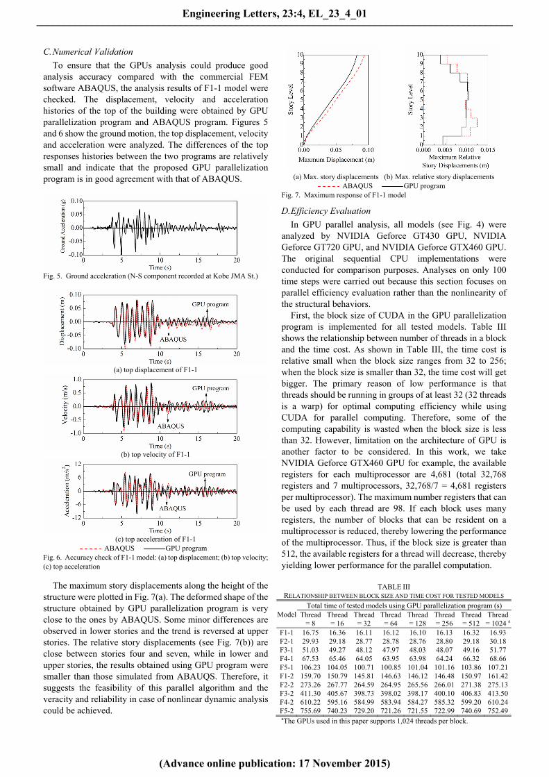
C. Numerical Validation

To ensure that the GPUs analysis could produce good analysis accuracy compared with the commercial FEM software ABAQUS, the analysis results of F1-1 model were checked. The displacement, velocity and acceleration histories of the top of the building were obtained by GPU parallelization program and ABAQUS program. Figures 5 and 6 show the ground motion, the top displacement, velocity and acceleration were analyzed. The differences of the top responses histories between the two programs are relatively small and indicate that the proposed GPU parallelization program is in good agreement with that of ABAQUS.

Fig. 5. Ground acceleration (N-S component recorded at Kobe JMA St.)

(a) top displacement of F1-1

(b) top velocity of F1-1

(c) top acceleration of F1-1

ABAQUS GPU program Fig. 6. Accuracy check of F1-1 model: (a) top displacement; (b) top velocity; (c) top acceleration

The maximum story displacements along the height of the structure were plotted in Fig. 7(a). The deformed shape of the structure obtained by GPU parallelization program is very close to the ones by ABAQUS. Some minor differences are observed in lower stories and the trend is reversed at upper stories. The relative story displacements (see Fig. 7(b)) are close between stories four and seven, while in lower and upper stories, the results obtained using GPU program were smaller than those simulated from ABAUQS. Therefore, it suggests the feasibility of this parallel algorithm and the veracity and reliability in case of nonlinear dynamic analysis could be achieved.

(a) Max. story displacements (b) Max. relative story displacements

ABAQUS GPU program Fig. 7. Maximum response of F1-1 model

D. Efficiency Evaluation

In GPU parallel analysis, all models (see Fig. 4) were analyzed by NVIDIA Geforce GT430 GPU, NVIDIA Geforce GT720 GPU, and NVIDIA Geforce GTX460 GPU. The original sequential CPU implementations were conducted for comparison purposes. Analyses on only 100 time steps were carried out because this section focuses on parallel efficiency evaluation rather than the nonlinearity of the structural behaviors.

First, the block size of CUDA in the GPU parallelization program is implemented for all tested models. Table III shows the relationship between number of threads in a block and the time cost. As shown in Table III, the time cost is relative small when the block size ranges from 32 to 256; when the block size is smaller than 32, the time cost will get bigger. The primary reason of low performance is that threads should be running in groups of at least 32 (32 threads is a warp) for optimal computing efficiency while using CUDA for parallel computing. Therefore, some of the computing capability is wasted when the block size is less than 32. However, limitation on the architecture of GPU is another factor to be considered. In this work, we take NVIDIA Geforce GTX460 GPU for example, the available registers for each multiprocessor are 4,681 (total 32,768 registers and 7 multiprocessors, 32,768/7 = 4,681 registers per multiprocessor). The maximum number registers that can be used by each thread are 98. If each block uses many registers, the number of blocks that can be resident on a multiprocessor is reduced, thereby lowering the performance of the multiprocessor. Thus, if the block size is greater than 512, the available registers for a thread will decrease, thereby yielding lower performance for the parallel computation.

TABLE III

RELATIONSHIP BETWEEN BLOCK SIZE AND TIME COST FOR TESTED MODELS

ModelTotal time of tested models using GPU parallelization program (s)

Thread = 8

Thread = 16

Thread = 32

Thread = 64

Thread = 128

Thread = 256

Thread = 512

Thread = 1024 a

F1-1 16.75 16.36 16.11 16.12 16.10 16.13 16.32 16.93 F2-1 29.93 29.18 28.77 28.78 28.76 28.80 29.18 30.18 F3-1 51.03 49.27 48.12 47.97 48.03 48.07 49.16 51.77 F4-1 67.53 65.46 64.05 63.95 63.98 64.24 66.32 68.66 F5-1 106.23 104.05 100.71 100.85 101.04 101.16 103.86 107.21 F1-2 159.70 150.79 145.81 146.63 146.12 146.48 150.97 161.42 F2-2 273.26 267.77 264.59 264.95 265.56 266.01 271.38 275.13 F3-2 411.30 405.67 398.73 398.02 398.17 400.10 406.83 413.50 F4-2 610.22 595.16 584.99 583.94 584.27 585.32 599.20 610.24F5-2 755.69 740.23 729.20 721.26 721.55 722.99 740.69 752.49aThe GPUs used in this paper supports 1,024 threads per block.



______________________________________________________________________________________

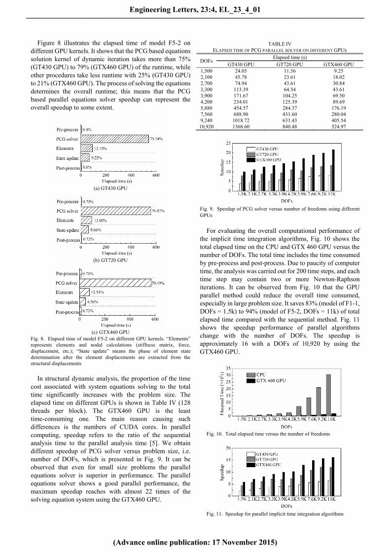
Figure 8 illustrates the elapsed time of model F5-2 on different GPU kernels. It shows that the PCG based equations solution kernel of dynamic iteration takes more than 75% (GT430 GPU) to 79% (GTX460 GPU) of the runtime, while other procedures take less runtime with 25% (GT430 GPU) to 21% (GTX460 GPU). The process of solving the equations determines the overall runtime; this means that the PCG based parallel equations solver speedup can represent the overall speedup to some extent.

(a) GT430 GPU

(b) GT720 GPU

(c) GTX460 GPU

Fig. 8. Elapsed time of model F5-2 on different GPU kernels. “Elements” represents elements and nodal calculations (stiffness matrix, force, displacement, etc.); “State update” means the phase of element state determination after the element displacements are extracted from the structural displacements

In structural dynamic analysis, the proportion of the time

cost associated with system equations solving to the total time significantly increases with the problem size. The elapsed time on different GPUs is shown in Table IV (128 threads per block). The GTX460 GPU is the least time-consuming one. The main reason causing such differences is the numbers of CUDA cores. In parallel computing, speedup refers to the ratio of the sequential analysis time to the parallel analysis time [5]. We obtain different speedup of PCG solver versus problem size, i.e. number of DOFs, which is presented in Fig. 9. It can be observed that even for small size problems the parallel equations solver is superior in performance. The parallel equations solver shows a good parallel performance, the maximum speedup reaches with almost 22 times of the solving equation system using the GTX460 GPU.

TABLE IV

ELAPSED TIME OF PCG PARALLEL SOLVER ON DIFFERENT GPUS

DOFsElapsed time (s)

GT430 GPU GT720 GPU GTX460 GPU 1,500 24.05 11.56 9.25 2,100 45.78 23.61 18.02 2,700 74.94 43.61 30.84 3,300 113.39 64.54 43.61 3,900 171.67 104.25 69.50 4,200 234.01 125.39 89.69 5,880 454.57 284.37 176.19 7,560 688.90 431.60 280.04 9,240 1018.72 631.43 405.54 10,920 1368.60 840.48 524.97

Fig. 9. Speedup of PCG solver versus number of freedoms using different GPUs

For evaluating the overall computational performance of

the implicit time integration algorithms, Fig. 10 shows the total elapsed time on the CPU and GTX 460 GPU versus the number of DOFs. The total time includes the time consumed by pre-process and post-process. Due to paucity of computer time, the analysis was carried out for 200 time steps, and each time step may contain two or more Newton-Raphson iterations. It can be observed from Fig. 10 that the GPU parallel method could reduce the overall time consumed, especially in large problem size. It saves 83% (model of F1-1, DOFs = 1.5k) to 94% (model of F5-2, DOFs = 11k) of total elapsed time compared with the sequential method. Fig. 11 shows the speedup performance of parallel algorithms change with the number of DOFs. The speedup is approximately 16 with a DOFs of 10,920 by using the GTX460 GPU.

Fig. 10. Total elapsed time versus the number of freedoms

Fig. 11. Speedup for parallel implicit time integration algorithms



______________________________________________________________________________________

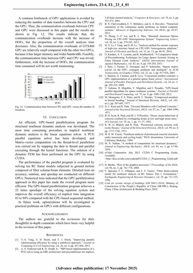
A common bottleneck of GPU applications is avoided by reducing the number of data transfers between the CPU and the GPU. Thus, the communication overheads between CPU and GPU were discussed in this paper and the results are shown in Fig. 12. The results indicate that, the communication overheads increase with the increase of DOFs, but the proportion of the overall analysis time decreases. Also, the communication overheads of GTX460 GPU are relatively small compared with the other two GPUs, because it has larger memory and wider bandwidth. Feasibly, the communication time between GPU and CPU was trivial; furthermore, with the increase of DOFs, the communication time consumed will be not worth mentioning.

Fig. 12. Communication time between CPU and GPU versus the number of freedoms

VI. CONCLUSION

An efficient, GPU-based parallelization program for structural nonlinear dynamic analysis was developed. The most time consuming procedure in implicit nonlinear dynamic analysis is the linear equations solver. A PCG parallel equations solver has been developed, and Matrix-vector computation via the thread-level parallelism was carried out by mapping the data to thread and parallel executing through the kernel functions. The solution of a dynamic FEM has been performed on the GPU by using CUDA.

The performance of the parallel program is evaluated by solving ten RC frame models subjected to ground motion composed of fiber column-beam elements. Detailed tests on accuracy, runtime, and speedup are conducted on different GPUs. Numerical tests indicated that the GPU parallelization approach in this paper has made the overall program more efficient. The GPU-based parallelization program achieves a 22 times speedups of the solving equation system and improves the overall efficiency of implicit time integration 83 to 94% compared with the CPU-based sequential method.

In future work, optimizations will be investigated in practical problems on GPUs with different configurations.

ACKNOWLEDGMENT

The authors are grateful to the reviewers for their thoughtful in-depth comments which have been very helpful in the revision of this paper.

REFERENCES [1] Y.-S. Yang, S. H. Hsieh, and T. J. Hsieh, “Improving parallel

substructuring efficiency by using a multilevel approach,” Journal of Computing in Civil Engineering, vol. 26, no. 4, pp. 457-464, 2012.

[2] A. S. Gullerud and R. H. Dodds Jr., “MPI-based implementation of a PCG solver using an EBE architecture and preconditioner for implicit,

3-D finite element analysis,” Computers & Structures, vol. 79, no. 5, pp. 553-575, 2001.

[3] B. N. Chetverushkin, E. V. Shilnikov, and A. A. Davydov, “Numerical simulation of the continuous media problems on hybrid computer systems,” Advances in Engineering Software, vol. 60-61, pp. 42-47, 2013.

[4] N. Zhang, C.-U. Lei, and K. L. Man, “Binomial American Option Pricing on CPU-GPU Heterogeneous System,” Engineering Letters, vol. 20, no. 3, pp. 279-285, 2012.

[5] H.-Y. Li, J. Teng, and Z.-H. Li, “Analysis method for seismic response of high-rise structure based on CPU-GPU heterogeneous platform,” Journal of Vibration and Shock, vol. 33, no. 13, pp. 86-91, 2014.

[6] O. Kardani, A. V. Lyamin, and K. Krabbenhoft, “A Comparative Study of Preconditioning Techniques for Large Sparse Systems Arising in Finite Element Limit Analysis,” IAENG International Journal of Applied Mathematics, vol. 43, no. 4, pp. 195-203, 2013.

[7] J. Bolz, I. Farmer, E. Grinspun, and P. Schröoder, “Sparse matrix solvers on the GPU: conjugate gradients and multigrid,” in ACM Transactions on Graphics (TOG), vol. 22, no. 3, pp. 917-924, 2003.

[8] L. Buatois, G. Caumon, and B. Levy, “Concurrent number cruncher: a GPU implementation of a general sparse linear solver,” International Journal of Parallel, Emergent and Distributed Systems, vol. 24, no. 3, pp. 205-223, 2009.

[9] V. Galiano, H. Migallón, V. Migallón, and J. Penadés, “GPU-based parallel algorithms for sparse nonlinear systems,” Journal of Parallel and Distributed Computing, vol. 72, no. 9, pp. 1098-1105, 2012.

[10] M. Menegotto, P. E. Pinto, and R. C. Slender, “Compressed members in biaxial bending,” Journal of Structural Division, ASCE, vol. 103, no.3, pp. 587-605, 1977.

[11] D. C. Kent and R. Park, “Flexural Members with Confined Concrete,” Journal of the Structural Division, ASCE, vol. 97, no. 7, pp. 1969-1990, 1971.

[12] B. D. Scott, R. Park, and M. J. N Priestley, “Stress–strain behaviour of concrete confined by overlapping hoops at low and high strain rates,” ACI Journal, vol. 79, no. 1, pp. 13–27, 1982.

[13] R. W. G. Blakely and R. Park, “Prestressed concrete sections with cyclic flexure,” Journal of the Structural Division, ASCE, vol. 99, no. 8, pp. 1717-1742, 1973．

[14] M. H. M. Yassin, “Nonlinear analysis of prestressed concrete structures under monotonic and cycling loads,” Ph.D. dissertation, University of California, Berkeley, 1994.

[15] M. N. Nathan, “A method of computation for structural dynamics,” Journal of Engineering Mechanics, ASCE, vol. 85, no. 3, pp. 67-94, 1959.

[16] nVidai Corporation. July 2013. CUDA C Programming Guide. Available: <http://docs.nvidia.com/cuda/pdf/CUDA_C_Programming_Guide.pdf>

[17] D. Blythe, “Rise of the graphics processor,” Proceedings of the IEEE, vol. 96, no. 5, pp. 761-778, 2008.

[18] E. Spacone, F. C. Fillippou, and F. F. Taucer, “Fiber beam-column model for nonlinear analysis of RC frames: Part I. Formulation,” Earthquake Engineering & Structure Dynamics, vol. 25, pp. 711-725, 1996.

[19] Code for seismic design of buildings (GB 50011-2010), Ministry of Construction of the People’s Republic of China (MCPRC), Beijing, China: China Architecture & Building Press, 2010.



______________________________________________________________________________________

nonlinear dynamic analysis efficiency by using a … · with that obtained by abaqus. ... nonlinear...

Documents