nonlinear digital encoders for data communications
TRANSCRIPT


Nonlinear Digital Encoders for Data Communications

FOCUS SERIES
Series Editor Francis Castanié
Nonlinear Digital Encodersfor Data Communications
Călin VlădeanuSafwan El Assad
First published 2014 in Great Britain and the United States by ISTE Ltd and John Wiley & Sons, Inc.
Apart from any fair dealing for the purposes of research or private study, or criticism or review, aspermitted under the Copyright, Designs and Patents Act 1988, this publication may only be reproduced,stored or transmitted, in any form or by any means, with the prior permission in writing of the publishers,or in the case of reprographic reproduction in accordance with the terms and licenses issued by theCLA. Enquiries concerning reproduction outside these terms should be sent to the publishers at theundermentioned address:
ISTE Ltd John Wiley & Sons, Inc.27-37 St George’s Road 111 River StreetLondon SW19 4EU Hoboken, NJ 07030UK USA
www.iste.co.uk www.wiley.com
© ISTE Ltd 2014The rights of Călin Vlădeanu and Safwan El Assad to be identified as the authors of this work have beenasserted by them in accordance with the Copyright, Designs and Patents Act 1988.
Library of Congress Control Number: 2013956557
British Library Cataloguing-in-Publication DataA CIP record for this book is available from the British LibraryISSN 2051-2481 (Print)ISSN 2051-249X (Online)ISBN 978-1-84821-649-5
Printed and bound in Great Britain by CPI Group (UK) Ltd., Croydon, Surrey CR0 4YY
Table of Contents
Preface . . . . . . . . . . . . . . . . . . . . . . . . . . . . . . . . . . . . . ix
Introduction . . . . . . . . . . . . . . . . . . . . . . . . . . . . . . . . . xi
Chapter 1. Applications of Nonlinear Digital Encoders . . . . . . . . 1
1.1. Secure communications using nonlinear digital encoders . . . . 11.1.1. The general nonlinear digital encoder scheme . . . . . . . . 31.1.2. Quasi-chaotic sequence properties . . . . . . . . . . . . . . . 51.1.3. An example of simple nonlinear digital encoder: the Frey
chaotic encoder . . . . . . . . . . . . . . . . . . . . . . . . . 71.1.4. Simulation results revealing the quasi-chaotic properties for
the sequences generated using the Frey encoder . . . . . . . 91.2. Chaotic spreading sequences for direct-sequence code division
multiple access . . . . . . . . . . . . . . . . . . . . . . . . . . . . 151.3. Sequence synchronization in discrete-time nonlinear systems . . 19
1.3.1. An example of sequence synchronization using the inversesystem . . . . . . . . . . . . . . . . . . . . . . . . . . . . . . 19
1.3.2. The dead-beat synchronization method . . . . . . . . . . . . 231.3.3. A communication scheme using the dead-beat
synchronization . . . . . . . . . . . . . . . . . . . . . . . . . 25
Chapter 2. Presentation of the Frey Nonlinear Encoder as a DigitalFilter . . . . . . . . . . . . . . . . . . . . . . . . . . . . . . . . . . . . . . 29
2.1. The mathematical analysis of the Frey encoder . . . . . . . . . . 29
vi Nonlinear Digital Encoders for Data Communications
2.2. The definitions and properties of the unsignedand 2’s complement signed sample operators . . . . . . . . . . . 30
2.3. The properties of the LCIRC nonlinear function used in the Freyencoder scheme . . . . . . . . . . . . . . . . . . . . . . . . . . . 38
2.4. The simulation of the Frey sequence generator block inSimulink: some practical considerations . . . . . . . . . . . . . 41
2.4.1. The transmitter chaotic sequence generator . . . . . . . . . . 412.4.2. The receiver chaotic sequence generator and the dead-beat
synchronization with the transmitter block . . . . . . . . . . 432.4.3. The Simulink implementations for the blocks used in the
Frey chaotic codec . . . . . . . . . . . . . . . . . . . . . . . 45
Chapter 3. Trellis-Coded Modulation Schemes Using NonlinearDigital Encoders . . . . . . . . . . . . . . . . . . . . . . . . . . . . . . . 49
3.1. The presentation of the Frey nonlinear encoder as aconvolutional encoder . . . . . . . . . . . . . . . . . . . . . . . . 49
3.2. Frey encoder trellis design optimization methods for pulseamplitude – trellis-coded modulation (TCM) schemes . . . . . . 54
3.2.1. Increasing the coding gain by reducing the representationcode word length in the input . . . . . . . . . . . . . . . . . 56
3.2.2. Equivalence between a nonlinear and a linear encoder in aparticular case . . . . . . . . . . . . . . . . . . . . . . . . . . 66
3.2.3. Generalized optimum encoder for a PAM-TCM transmission 693.2.4. Increasing the coding gain by increasing the number of
outputs . . . . . . . . . . . . . . . . . . . . . . . . . . . . . . 753.3. Optimum nonlinear encoders for phase shift keying – TCM
schemes . . . . . . . . . . . . . . . . . . . . . . . . . . . . . . . . 843.3.1. Rate-1/2 optimum encoder for a QPSK-TCM transmission . 843.3.2. Generalized optimum encoder for a PSK-TCM transmission 85
3.4. Optimum nonlinear encoders for quadrature amplitudemodulation – TCM schemes . . . . . . . . . . . . . . . . . . . . 89
3.5. Performance analysis of TCM data communications usingmodified nonlinear digital encoders: simulation results . . . . . 91
Chapter 4. Parallel Turbo Trellis-Coded Modulation Schemes UsingNonlinear Digital Encoders . . . . . . . . . . . . . . . . . . . . . . . . 97
4.1. Recursive convolutional-left circulate (RC-LCIRC) encoder ina turbo trellis-coded modulation (TTCM) scheme . . . . . . . . 97
Table of Contents vii
4.2. New recursive and systematic convolutional nonlinear encodersfor parallel TTCM schemes . . . . . . . . . . . . . . . . . . . . . 100
4.3. Punctured TTCM transmissions using recursive systematicconvolutional nonlinear encoders . . . . . . . . . . . . . . . . . . 108
4.4. Extrinsic information transfer (EXIT) charts analysis for TTCMschemes using nonlinear RSC encoders . . . . . . . . . . . . . . 114
4.5. Performance analysis of TTCM data communications usingnonlinear digital encoders: simulation results . . . . . . . . . . . 115
Appendix . . . . . . . . . . . . . . . . . . . . . . . . . . . . . . . . . . . 133
Bibliography . . . . . . . . . . . . . . . . . . . . . . . . . . . . . . . . . 145
Index . . . . . . . . . . . . . . . . . . . . . . . . . . . . . . . . . . . . . . 151

Preface
Several applications using nonlinear dynamical systems have beendeveloped over the last few decades. Among these, the field oftelecommunications has clearly benefited from these nonlinear blocks. Hence,the nonlinear blocks have proved to be suitable for implementing severaltelecommunications techniques, such as encryption, spectrum spreading andchannel coding.
In this book, we present novel solutions for channel coding using nonlinearsequence generators. To the best of our knowledge, there are only a few worksthat attempt to propose the use of nonlinear functions for channel coding intelecommunications systems. In this context, this book aims to demonstratethat nonlinear encoders can be designed to provide good performances and toencourage researchers to investigate these approaches further.
This book contains many numerical examples that complete thedescription of the analyzed schemes. Also, some performance simulationresults are provided. Some sections include presentations of the mathematicalapparatus used throughout the book and some Matlab/Simulink scripts andschemes used to run the simulations.
We recommend this book to students, especially for Master’s and PhDstudents who will easily understand the concepts presented in this book andcan design and test these schemes by simulations.

x Nonlinear Digital Encoders for Data Communications
We also consider that this book may be used by telecommunicationsengineers to complete their grounding in the field of signal processing fortelecommunications, especially on non-conventional and nonlinear codedmodulation techniques.
Calin VLADEANU
Safwan EL ASSAD
January 2014
Introduction
During the last few decades, several chaotic sequence generators have beeninvestigated for secure and efficient digital communication systems. Becauseof their generators’ sensitive dependence on the initial state, these sequencespresent pseudo-random properties and offer an enhanced security.
As is well known, chaotic sequence generators are nonlinear dynamicalsystems and their finite precision or quantized approximations affect thechaotic regimes. Hence, this problem can be overcome by developing digitalgenerators. In [FRE 93], Frey proposed a chaotic digital infinite impulseresponse (IIR) filter for a secure communications system. The Frey filtercontains a nonlinear function called the left-circulate (LCIRC) function,which provides the chaotic properties of the filter. The LCIRC functionperforms a bit left circulation over the N bits representation word. In thesame paper, Frey showed that this nonlinear recursive filter possessesquasi-chaotic properties, both for autonomous and non-autonomous modes.In [WER 98], Werter improved this encoder in order to increase therandomness between the output sequence samples. The performances of apulse amplitude modulation (PAM) communication system using the Freyencoder, with additive white Gaussian noise (AWGN), were analyzed in[AIS 96]. A modified state feedback decoder was proposed in [AIS 96] andperforms better than the Frey inverse filter decoder, in terms of bit error rate(BER) at a high signal-to-noise ratio (SNR).
In all these previous works, the Frey encoder has been considered as adigital filter, operating over Galois field GF 2N and was used to increase thesecurity of the transmissions. During the last few decades, the nonlinear
xii Nonlinear Digital Encoders for Data Communications
functions have been used extensively in chaotic sequence generators toincrease the security of communications systems.
Nowadays, channel-encoded transmissions are used in all systems. Severaltypes of channel encoding methods have been proposed during the last fewdecades. Almost all coding methods known in the literature use linearfunctions. Barbulescu et al. made one of the first approaches regarding thepossible use of the Frey encoder in a turbo-coded communication system[BAR 00]. Nevertheless, in [BAR 00], the authors only mentioned as anadvantage the intrinsic randomness of the encoder, which eliminates the useof an interleaver from the typical turbo encoding/decoding schemes. Despitethe promising idea, this book did not consider any information theoryapproach for performance evaluation and, above all, it did not prove theadvantages of these turbo encoders. In [ZHO 01], Zhou et al. made a similaranalysis and again, the paper lacks proof for the stated performanceenhancement. Another more recent work [NG 08] addressed differentmethods for using chaotic sequence generators to enhance the coding gain orthe security of several coded schemes. More recently, in [ESC 09], a turbotrellis-coded modulation (TTCM) scheme using digital chaotic encoders withbinary inputs and chaotic outputs is proposed. This work and the referencestherein introduce a different family of nonlinear encoders than the encodersanalyzed in this book. However, we consider that the work of Escribano et al.[ESC 09] presents many similarities to our work, especially in the encoders’design and performance analysis solutions.
In [VLA 09a], a different perspective was offered for the chaotic digitalencoder proposed by Frey in [FRE 93]. Mainly, it was observed that thisencoder with finite precision possesses a trellis that describes its deterministicfunctioning. This led to the possibility of improving the performances of thechaotic sequence transmission over a noisy channel by using sequencedetection. In fact, this is the reason why this encoder should perform well inturbo coding schemes. To demonstrate this performance improvement ascompared to the non-encoded system, a new TCM scheme was developed forobtaining better performance in the presence of noise. This method partiallyfollows the rules proposed by Ungerboeck in [UNG 82] for defining optimumTCMs by proper set partitioning (SP). The main idea is to use a differentword length in the output as compared to the input. In [CLE 06], Clevomet al. developed a method for separating a recursive systematic convolutional(RSC) encoder into subencoders with only a single delay element. This
Introduction xiii
equivalency makes a GF(2) RSC equivalent to a simpler RSC that worksinside over a higher order field, while its input and output still work overGF(2). Even if a different problem was addressed in [CLE 06], this idea ledto the fact that different representation word lengths can be used in the inputand output, and a higher order field nonlinear encoder is equivalent to a linearGF(2) RSC encoder. Therefore, in [VLA 09a], it was demonstrated that theFrey encoder with finite precision (word length of N bits) presented in[FRE 93] is a recursive convolutional (RC), but non-systematic, encoderoperating over GF 2N . In the same work [VLA 09a], a new method isproposed for enhancing the performances of the chaotic PAM-TCMtransmission over a noisy channel.
A generalization of the optimum one-delay GF(4) encoder in [VLA 09a]was made, for any output word length N and for any possible encoding rate,in the cases of PAM-TCM [VLA 09b] and phase-shift keying TCM(PSK-TCM) [VLA 10b] transmission schemes. The development of optimumGF 2N encoders for the quadrature amplitude modulation (QAM) TCMscheme is more difficult than in the case of PAM and PSK modulations, dueto the larger constellations and non-uniform power per symbol. In[VLA 11b], a generalization of the optimum one-delay GF(4) encoder in[VLA 09a] is performed, for any output word length N and for any possibleencoding rate in QAM-TCM schemes. These encoders follow the rulesproposed by Ungerboeck [UNG 82] for defining optimum TCM by proper SP.However, all the previously mentioned encoders are non-systematic, makingthem unfeasible for TTCM schemes.
Two-dimensional (2D) TCM schemes using a different trellis optimizationmethod for Frey encoder were proposed in [VLA 09c]. Hence, the filterscheme is modified to have an additional output, which transforms it into arate 1/2 encoder. The second output is derived in such a manner as to transmita 2D TCM signal, following the Ungerboeck SP rules [UNG 82]. Despitethese changes, the filter representation word length is not changed.
The coding gain was estimated theoretically for all the consideredencoders, for different values of N . In fact, exact expressions of the minimumEuclidean distance were determined for all these TCM schemes. Freyencoders with small representation word length (N = 1 and N = 2) wereconsidered for simulations. There are two reasons for simulating encoderswith small word lengths. First, the trellis size increases exponentially with N ;
xiv Nonlinear Digital Encoders for Data Communications
second, the coding gain reduces when the word length increases. This lastproperty is explained by the fact that the increase in the constellation sizedecreases the signal minimum Euclidean distance, more than the encodingcan cope with. It is also noted that the linear encoders corresponding to theconsidered nonlinear encoders (obtained by eliminating the nonlinear block)do not have good trellises. For all these schemes, the simulated performancesconfirm the theoretically determined Euclidean distances.
The turbo coding scheme introduced by Berrou and Glavieux in theirseminal paper [BER 96] allows communications systems’ performances closeto the Shannon limit, by concatenating in parallel RC encoders in thetransmitter and using iterative decoding algorithms in the receiver. Turboschemes were developed for the TCM schemes as well [OGI 01, ROB 98].
In [PAU 10a], the RC-LCIRC encoder from [VLA 10b] is adapted for, andintroduced into, a parallel turbo PSK-TCM transmission scheme, and theperformances of this scheme are analyzed in case of transmitting over achannel with AWGN. Similarly, in [PAU 10b], the same RC-LCIRC isintroduced into a parallel turbo QAM. The QAM-TCM transmission schemeand the performances of this scheme are analyzed in case of transmitting overa channel with AWGN. The performances of the RC-LCIRC-TTCM schemesintroduced in [PAU 10a] and [PAU 10b] were analyzed in [VLA 10a]assuming a transmission over a non-selective Rayleigh fading channel.
In [VLA 11a], an improved version of the RC-LCIRC encoder from[VLA 10b] is proposed. The main encoder improvement consists of making itsystematic. In fact, this was the only disadvantage of the previous LCIRCencoders which were not fully compatible with the corresponding binaryencoders. Further to this new advantage, the encoder designing process aimedto keep all previous advantages of the LCIRC encoders, such as optimumperformances in terms of Euclidean distance, the reduced complexity in thememory usage (for any encoding rate, only one delay element is used) and acompact expression of the Euclidean distance for a specific modulation. Theoptimum SP method is used both for PSK and QAM-TCM schemes. Thesymbol error rate (SER) performances of these new schemes are analyzed incase of transmitting over a channel with AWGN. Corresponding binaryencoders, i.e. with the same values for the encoding rate, the number of trellisstates and the minimum Euclidean distance, are considered as a reference forSER comparison.
Introduction xv
A family of nonlinear encoders for the TTCM scheme was analyzed in[VLA 11c]. The systematic encoders introduced in [VLA 11a] were adaptedfor a parallel TTCM transmission scheme. As compared to the TTCM schemeanalyzed in [PAU 10b] operating at low coding rates due to the lack ofpuncturing, the work in [VLA 11c] introduces specific interleaving andpuncturing methods for the TTCM scheme. Moreover, the conventionallogarithmic maximum a posteriori probability (log-MAP) decoding algorithmis modified to operate in a symbol-by-symbol manner for punctured receivedsequences, following the method presented in [ROB 98] and [VUC 00]. Theoptimum SP method is used for PSK punctured TTCM schemes. Theperformances of this scheme are analyzed in case of transmitting over achannel with AWGN.
The work in [VLA 12] extends the performance analysis for thesenonlinear TTCM schemes. The extrinsic information transfer (EXIT) chart isan important tool for visualizing the exchange of the extrinsic informationbetween constituent decoders in a turbo receiver scheme [TEN 01]. Moreover,the EXIT charts are presented to underline the convergence behavior of theseschemes. The EXIT chart was also applied to TTCM schemes to depict thedecoding trajectory, allowing the prediction of BER waterfall and BER floorregions [CHE 04, KLI 06]. Two channel models were considered for theperformance analysis, i.e. the AWGN noisy channel and the Rayleigh fadingchannel. Also, the considered multilevel modulation techniques were PSKand QAM. Therefore, the EXIT chart can be used as a tool in the design ofTTCM schemes [NG 08].
The book is organized as follows. In Chapter 1, the nonlinear digitalencoders are introduced and their main applications for telecommunicationsare presented and discussed. In section 1.1, the general nonlinear digitalencoder scheme is presented, as it was introduced in the literature for securecommunications applications. This structure generates quasi-chaoticsequences that are suitable for such secure communications applications.Here, an example of a nonlinear codec introduced by Frey is analyzed andsimulations reveal its quasi-chaotic features. In section 1.2, the possible use ofthese structures in spread-spectrum applications is briefly discussed. A majorproblem arising from the use of discrete-time nonlinear systems intelecommunications is the sequence synchronization in the receiver part. Thisissue is addressed in section 1.3 for the particular case of the Henondiscrete-time map. Here, an efficient method for sequence synchronization,
xvi Nonlinear Digital Encoders for Data Communications
i.e. the dead-beat method, is presented and analyzed both theoretically and bymeans of simulations.
Chapter 2 is dedicated to the presentation of the Frey nonlinear encoderintroduced in section 1.1. To be more specific, in section 2.1, the Frey encoderis mathematically described using the modulo-2N operators. The propertiesof these operators are thoroughly analyzed in section 2.2. The demonstrationsfor some of the theorems given in section 2.2 are presented in the appendix.Using the operators introduced in section 2.2, the properties of the LCIRCfunction are demonstrated in section 2.3. Finally, taking advantage of themathematical development from the previous sections, the Matlab/Simulinksimulation block schemes for the Frey digital encoder, decoder, including thedead-beat synchronization method (described in section 1.3), are presented insection 2.4.
Chapter 3 presents the Frey encoder from a different perspective, i.e. as aconvolutional encoder. In section 3.1, the original Frey encoder is analyzed asa convolutional encoder and it is shown that it is not efficient for channelcoding. Two new PAM-TCM schemes for the Frey encoder are introduced insection 3.2. First, the trellis optimization method by reducing the inputrepresentation word length is presented for a particular case, and then it isgeneralized for any output word length value. Hence, a generalized optimumnonlinear RC encoder scheme is proposed and an expression is provided forthe minimum Euclidean distance of these encoders in a PAM-TCMtransmission. Also, the second PAM-TCM modified Frey scheme ispresented, which optimizes the coding performances by increasing thenumber of outputs, without modifying the input and output word lengths.Using a similar input word length optimization, a generalized optimumGF 2N RC encoder scheme is proposed and an expression is provided forthe minimum Euclidean distance of these encoders for a PSK-TCMtransmission in section 3.3 and for a QAM-TCM transmission in section 3.4.The simulated SER performance is presented in section 3.5 for the optimumPAM-TCM, PSK-TCM and QAM-TCM transmissions.
Chapter 4 analyzes the parallel TTCM schemes including convolutionalLCIRC encoders. First, in section 4.1, the RC-LCIRC encoder introduced inChapter 3 is used as a constituent encoder for non-punctured parallel PSK andQAM-TTCM schemes. A multilevel log-MAP algorithm is used for theiterative detection. The non-systematic nature of the RC-LCIRC encoder and
Introduction xvii
its effect on the TTCM scheme performances are pointed out. Therefore,section 4.2 presents the new generalized RSC-LCIRC encoder operating overGalois field GF 2N and the optimum SP for two-dimensional TCMschemes. In section 4.3, a parallel TTCM transmission scheme usingRSC-LCIRC component encoders with symbol puncturing is presented. Asymbol-by-symbol log-MAP algorithm is used for the iterative detection. Forthe constituent RSC-LCIRC encoders, the minimum Euclidean distance,minimum effective length and product distance are estimated for the AWGNchannel and the Rayleigh fading channel, respectively. The method used toplot the EXIT charts of these TTCM schemes is described in section 4.4. Thesimulated BER performance graphs and EXIT charts for the TTCM schemesintroduced in previous sections are presented in section 4.5. First, thesimulated BER performance over AWGN and Rayleigh fading channels isplotted for the 8-PSK-TTCM and 16-QAM-TTCM transmission schemesfrom section 4.1, using three types of mappings: Gray, natural and SP. Thecoding gains of these schemes using different mappings, as compared to theuncoded modulation and the non-iterative schemes, are derived fromsimulations. Next, the SER performances are plotted for optimum 8-PSK and16-QAM RSC-LCIRC-TCM transmissions over an AWGN channel, using theencoder introduced in section 4.2. Finally, the simulated BER performancesin AWGN and Rayleigh fading channels are presented and analyzed for thepunctured 8-PSK and 16-QAM-TTCM transmission using three differentinterleaver sizes. Also, the EXIT charts are plotted to compare theconvergence of different TTCM decoding schemes for the punctured 8-PSKand 16-QAM-TTCM transmissions.

1
Applications of Nonlinear Digital Encoders
1.1. Secure communications using nonlinear digital encoders
Recently, interest has been growing in the use of chaos for securecommunications. Spread-spectrum communications are included in thecategory of secure communications, which also stand to benefit from thisresearch.
Using analog chaotic systems for secure communications schemes presentssome drawbacks for practical applications, since all show an intrinsic weakrobustness, i.e. the unavoidable errors on the values of the circuit components,as well as the disturbances generated by the communication link, can heavilyinfluence the synchronization process and can make it ineffective.
In general, three communication schemes have been proposed so far:chaotic switching where the information is binary and switches thetransmitted signal between two attractors, chaotic masking where theinformation is simply added to the chaotic signal and chaotic modulationwhere the information is “modulated” on a chaotic carrier by means of aninvertible nonlinear transformation. Researchers have shown experimentalprototype implementations of secure communication systems utilizing chaos.They capitalize upon the fact that chaotic circuits taken from an appropriateclass can be made to synchronize. Specifically, it has been shown [PEC 90]that if a chaotic system can be divided into subsystems with stable Lyapunovexponents, then it will asymptotically track a replica of itself. Kocarev et al.[KOC 92] and Cuomo and Oppenheim [CUO 93] demonstrate the fact thatthis tracking phenomenon is robust enough to allow locking to occur even in
2 Nonlinear Digital Encoders for Data Communications
the presence of a continuous perturbation. In particular, they add a small(12 dB down in [KOC 92] and 20 dB down in [CUO 93]) message signal tothe chaotic signal produced by a first chaotic circuit taken from the classdescribed above. This transmitted signal is then relayed to the receiver, wherean identical chaotic circuit locks onto the dominant chaotic component. Whena lock is achieved, the chaotic replica of the original chaotic signal issubtracted from the received composite signal, leaving the message signal.
A variation is studied in [CUO 93] and [PAR 92], where the messagesignal is a binary signal causing a parameter in the transmitting chaotic circuitto take on two possible values, thereby producing a modulated chaotic output.The receiver replica has the respective parameter fixed to one of the possiblevalues in its counterpart. As a result, it tracks the transmitter anytime thebinary input is one state and falls out of sync at times corresponding to theother input state. Lock and unlock conditions are easily detected, resulting inproper demodulation. An even more intriguing variation is proposed by Halleet al. [HAL 93], which is most closely related to the work presented in thefollowing, although it is analog. In [HAL 93], Chua’s circuit is driven by anexternal input that is a modulated version of the message signal. Themodulation is achieved via a nonlinear operation with the chaotic output ofthe circuit. Then, this output is fed to a copy of the chaotic circuit at thereceiver end, which synchronizes with the transmitter circuit and contains theinverse modulation function. It is demonstrated that this nonlinear modulationof the input with the chaotic signal produces a system whose encoded signalis quantitatively chaotic and that is sensitive to parameter mismatch betweenthe receiver and the transmitter, two qualities that are highly desirable for usein secure communications applications. The benefit of the encoding (ormodulation) schemes outlined above is that the transmitted signal issubstantially chaotic to an observer. Hence, in general, it would bear littleresemblance to the message signal, thereby producing a measure of securityin the transmission of the data. While all these approaches are fascinating andsurely warrant further investigation, they may suffer from serious drawbacksin practice. First, since two matched analog chaotic circuits are required atremote locations, in practice there can be serious problems with systemperformance unless a method of calibration is devised. On the other hand, therobustness of the tracking phenomena should allow some mismatch to occurwhile providing acceptable performance. However, this robustness could beexploited by an unintended listener diminishing the security of the system.
Applications of Nonlinear Digital Encoders 3
Another drawback to the additive approach [CUO 93, KOC 92], i.e. where themessage signal is added to the chaotic signal, is that the signal-to-noise ratioof the received signal is directly degraded by the chaos-to-signal ratio (12 dBin [KOC 92] and 20 dB in [CUO 93]) relative to available channelsignal-to-noise ratio. Furthermore, adaptive filtering techniques may allow anintruder to find the information in the chaotic noise, despite its overwhelmingmagnitude. Alternatively, in the binary modulation approach, it may bepossible to detect the binary signal without locking onto the chaotic signaldirectly, thereby compromising security.
1.1.1. The general nonlinear digital encoder scheme
In this section, we present the secure communications system proposed byFrey [FRE 93] that has all the advantages of any other chaos-based system,but also has other advantages, which are not present in previously proposedschemes. First, the system is digital, which makes a perfect reconstruction inthe receiver of the transmitted signal possible. Second, the system introducedby Frey produces transmitted signals with virtually no correlation to the input,while being substantially chaotic in appearance.
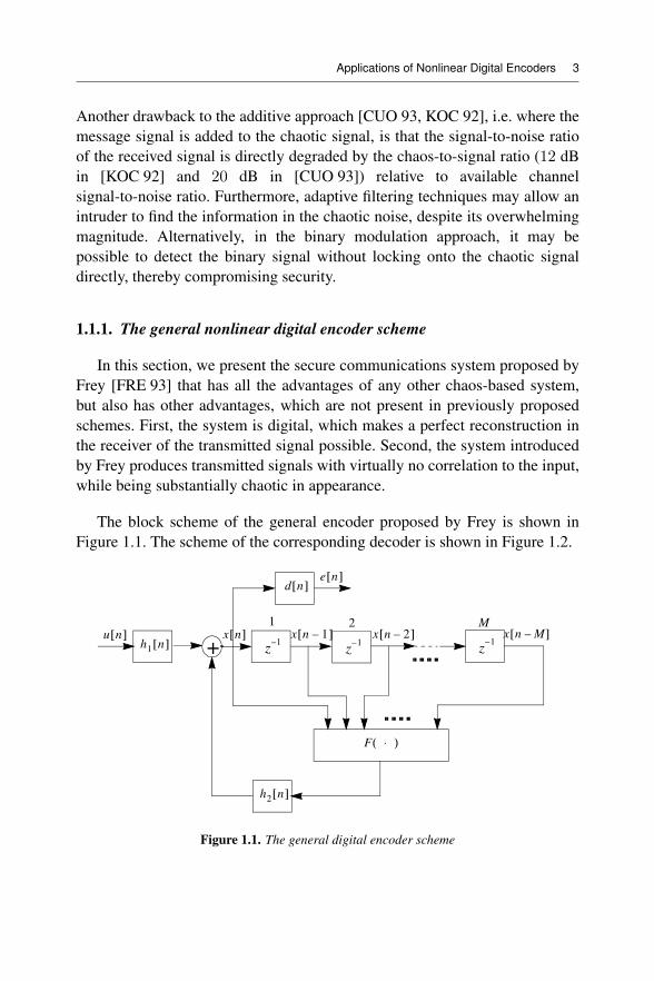
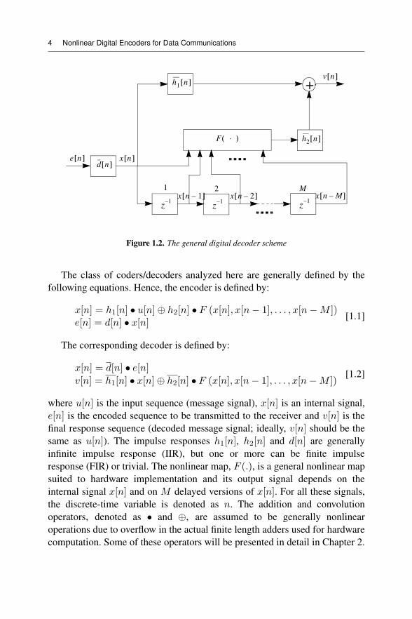
The block scheme of the general encoder proposed by Frey is shown inFigure 1.1. The scheme of the corresponding decoder is shown in Figure 1.2.
u n[ ] x n[ ]
+h1
n[ ]x n 1–[ ]
z1–
x n 2–[ ]
z1–
x n M–[ ]1 2 M
d n[ ]e n[ ]
F ⋅( )
z1–
h2
n[ ]
Figure 1.1. The general digital encoder scheme
4 Nonlinear Digital Encoders for Data Communications
+h1
n[ ]
x n 1–[ ]
z1–
x n 2–[ ]
z1–
x n M–[ ]1 2 M
d n[ ]x n[ ]
F ⋅( )
z1–
h2
n[ ]
e n[ ]
v n[ ]
Figure 1.2. The general digital decoder scheme
The class of coders/decoders analyzed here are generally defined by thefollowing equations. Hence, the encoder is defined by:
x[n] = h1[n] • u[n]⊕ h2[n] • F (x[n], x[n− 1], . . . , x[n−M ])e[n] = d[n] • x[n] [1.1]
The corresponding decoder is defined by:
x[n] = d[n] • e[n]v[n] = h1[n] • x[n]⊕ h2[n] • F (x[n], x[n− 1], . . . , x[n−M ])
[1.2]
where u[n] is the input sequence (message signal), x[n] is an internal signal,e[n] is the encoded sequence to be transmitted to the receiver and v[n] is thefinal response sequence (decoded message signal; ideally, v[n] should be thesame as u[n]). The impulse responses h1[n], h2[n] and d[n] are generallyinfinite impulse response (IIR), but one or more can be finite impulseresponse (FIR) or trivial. The nonlinear map, F (.), is a general nonlinear mapsuited to hardware implementation and its output signal depends on theinternal signal x[n] and on M delayed versions of x[n]. For all these signals,the discrete-time variable is denoted as n. The addition and convolutionoperators, denoted as • and ⊕, are assumed to be generally nonlinearoperations due to overflow in the actual finite length adders used for hardwarecomputation. Some of these operators will be presented in detail in Chapter 2.
Applications of Nonlinear Digital Encoders 5
The defining equations given by [1.1] allow for a very wide variety ofsystems. Note that the decoder must be a nonlinear filter that implements theinverse of the encoder for proper recovery of the input sequence, u[n]). Thisexplains why x[n] is assumed to be exactly recovered in the decoder as aninternal variable. The h1[n], h2[n] and d[n] blocks in the decoder scheme areconsidered as complementary to those in the encoder scheme (in the sense ofthe convolution operator, i.e. d[n] • d[n] = δ[n], where δ[n] is the Diracpulse). No general results, specific to the quasi-chaotic (QC) properties, onthis class of systems is available in the literature. While Chua and Lin[CHU 88, CHU 90] have given a very clever construction to prove theexistence of chaotic trajectories in second- and third-order filters, the discretenature of the systems considered in this work, coupled with the complexityassociated with non-autonomous responses, unfortunately seems to precludeany direct application of their method to the case discussed here. In an earlierwork [EBE 69], Ebert et al. have also suggested a method intuitively similarto the method in [CHU 88, CHU 90], but their results are aimed at basicallystable filters and the appearance of limit cycles. A mathematical analysis ofthe basic encoder of this chapter is presented in section 2.1, which drawsupon the work in [CHU 88, CHU 90] and [EBE 69], but only qualitativeresults are available at this time. The results shown in this work hopefullymake the pursuit of a complete theory more compelling.
1.1.2. Quasi-chaotic sequence properties
The presence of chaotic regimes in digital filters has been demonstrated byChua and Lin [CHU 88, CHU 90]. In these works, it was shown that theoverflow nonlinearity determines an otherwise linear digital filter to behavechaotically with certain initial conditions. The authors showed that the filterspresent the chaotic regimes, even in the more realistic situation where finiteword length is considered [LIN 91]. This fact is important, since, technically,all finite precision digital filters must possess periodic autonomous responses,thereby precluding the possibility of chaos. Nevertheless, the results in[LIN 91] give credence to the idea that practical digital filters can beessentially chaotic.
In fact, the regimes analyzed in [CHU 88, CHU 90, LIN 91] and [FRE 93]are not truly chaotic, because the digital filters possessing them work in finiteprecision. In [FRE 93], Frey introduces for the first time in the literature a
6 Nonlinear Digital Encoders for Data Communications
definition for a “quasi-chaotic behavior” by proposing a set of conditions thatmust be met by the filter response. This set of conditions, which is consistentwith the common observations about chaos, will be used as the criterion forwhether a chaotic response has been generated. This definition of a QC digitalfilter is provided below.
DEFINITION 1.1.– A QC digital filter is defined as a non-autonomous digitalfilter that possesses the following properties [FRE 93]:
1) the zero input response has a wideband noiselike spectrum for almostall choices of initial condition. Under the same conditions, the autocorrelationfunction of the response is similar to an uncorrelated noise sequence;
2) the response of the filter to arbitrary inputs has a broadband noiselikespectrum for almost all choices of initial conditions. Under the sameconditions, the autocorrelation function of the response is similar to anuncorrelated noise sequence;
3) the response of the filter to almost all arbitrary inputs is uncorrelated tothe input for almost all choices of initial conditions;
4) the responses of the filter to the same input sequences are uncorrelatedto one another for almost all choices of different initial conditions;
5) for almost all choices of input to two identical filters having different butarbitrarily close initial states, the states of the two filters will diverge.
The expression “almost all” used in properties 1–5 refers to the vastmajority (e.g. greater than 90% or 95%). Also, the term “noiselike” impliesnoise similar to a filtered version of white Gaussian noise. Theautocorrelation of the filter response has a maximum value in the origin, andvery low values elsewhere, while the period of the autocorrelation functiondepends on the length of cycles in the filter solution trajectories. Also, thecorrelation (intercorrelation) between two different responses, generated withdifferent initial conditions, takes low values as compared to the maximum inthe autocorrelation.
The empirically defined properties 1–5 [FRE 93] are useful for testing thechaotic behavior for any digital filter. Moreover, these properties areimportant for guaranteeing the security of a communication system using thechaotic filters possessing them. Even these properties were determined
Applications of Nonlinear Digital Encoders 7
empirically, an important number of tests were performed by simulation tocheck the validity of the properties [FRE 93]. Therefore, the conclusion isthat the QC properties do hold for even relatively simple filters. To verify thegenerality of these properties, we ran a significant number of tests to checkthem, following the same procedure as in [FRE 93]. The simulation results ofsuch tests confirm the validity of the QC properties. These results arepresented in section 1.1.4.
1.1.3. An example of simple nonlinear digital encoder: the Frey chaoticencoder
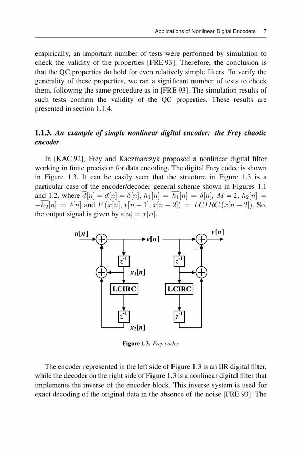
In [KAC 92], Frey and Kaczmarczyk proposed a nonlinear digital filterworking in finite precision for data encoding. The digital Frey codec is shownin Figure 1.3. It can be easily seen that the structure in Figure 1.3 is aparticular case of the encoder/decoder general scheme shown in Figures 1.1and 1.2, where d[n] = d[n] = δ[n], h1[n] = h1[n] = δ[n], M = 2, h2[n] =−h2[n] = δ[n] and F (x[n], x[n− 1], x[n− 2]) = LCIRC (x[n− 2]). So,the output signal is given by e[n] = x[n].
_
z-1
z-1
LCIRC
u[n]e[n]
x1[n]
x2[n]
z-1
z-1
LCIRC
v[n]
Figure 1.3. Frey codec
The encoder represented in the left side of Figure 1.3 is an IIR digital filter,while the decoder on the right side of Figure 1.3 is a nonlinear digital filter thatimplements the inverse of the encoder block. This inverse system is used forexact decoding of the original data in the absence of the noise [FRE 93]. The
8 Nonlinear Digital Encoders for Data Communications
first thing to note is that in real transmission systems, we always have noiseand a more realistic study is necessary assuming the presence of the noise. Itis also important to note that there is no internal feedback path in this decoder.Specifically, the decoder is an FIR nonlinear digital filter, which guaranteesthat an error in the communications channel, which can cause at most a finiteburst error in the output e[n].
Specifically, the system of Figure 1.3 follows these equations:
e[n] = u[n]⊕ {e[n− 1]⊕ f (e[n− 2])}v[n] = e[n] {e[n− 1]⊕ f (e[n− 2])} [1.3]
Let us assume that N denotes the word length used for binaryrepresentation of each sample. The encoder in Figure 1.3 is composed of twodelay elements with a sample interval, two modulo-2N adders and a nonlinearfunction called left-circulate (LCIRC), which is a function that is typicallyavailable as a basic accumulator operation in microprocessors. For furtherdetails on these modulo-2N operators, see section 2.2, while the LCIRCfunction properties are presented in section 2.3. In [1.3], the function f (.) isthe LCIRC function. For each sample moment n, u[n] represents the inputdata sample, x1[n] and x2[n] denote the delay elements’ states and e[n] is theoutput sample. The superscript U denotes that all the samples are representedin unsigned form, using N bits per word, i.e. uU [n], eU [n] ∈ 0, 2N − 1 .
The nonlinear LCIRC function is responsible for the QC behavior of thisencoder. Considering the unsigned modulo-2N operations, the LCIRC functionis defined in the following.
DEFINITION 1.2.– The LCIRC function consists of a multiplication by 2 plusthe carry bit. The LCIRC function is defined in the 2N -set, by the followingequation [FRE 93]:
yU [n] = LCIRC xU [n] = 2 ˙xU [n] + s[n] mod2N [1.4]
In [1.4], s[n] denotes the carry bit, which is given by:
s[n] =0 if 0 ≤ xU [n] ≤ 2N−1 − 11 if 2N−1 ≤ xU [n] ≤ 2N − 1
[1.5]
where xU , yU ∈ 0, 2N − 1 .
Applications of Nonlinear Digital Encoders 9
The LCIRC function defined by [1.4] and [1.5] is equivalent to thefollowing operations performed over the binary word unsignedrepresentation: denoting by N the word length used for binary representationof each sample, the LCIRC function performs a bit rotation by placing themost significant bit to the less significant bit and shifting the other N − 1 bitsone position to a higher significance. This is the reason why the function iscalled LCIRC. Analyzing the expression [1.5], we can note that besides thenonlinearity in the modulo-2N multiplications and additions, the carry bit s[n]also determines the nonlinearity of the LCIRC function, being related by anonlinear inequality with the input sample value.
In [KAC 92] and [FRE 93], it was demonstrated that the structure shownin Figure 1.3, which is defined by [1.3]–[1.5], possesses the QC propertiespresented in section 1.1.2. This was achieved by running extensivesimulations for a very large number of initial conditions. It was observed thatwith a constant input, the output was qualitatively chaotic for almost all setsof initial states in the delays. Chaos was qualitatively determined by verifyingthe QC properties introduced in section 1.1.2.
1.1.4. Simulation results revealing the quasi-chaotic properties for thesequences generated using the Frey encoder
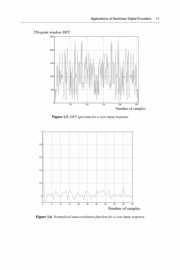
In this section, the QC properties of the system as shown in Figure 1.3 areverified following the same procedure as in [FRE 93]. First, it was noted thatthe richness of the dynamics is directly related to the word length. As in[FRE 93], the simulation results are determined for an 8-bit word length,which represents a compromise between complexity and the computationalburden of simulating the system over a wide variety of test conditions. Toinvestigate QC property 1, the zero input response was observed for allpossible choices of initial states. Almost all (> 98%) states were part ofcyclic responses of a period greater than 100. The longest cycle included37, 749 states and there were six other distinct cycles covering more than1, 000 states, namely 7, 063, 6, 594, 3, 392, 2, 601, 1, 343 and 1, 260. Betweenlength 100 and 1, 000 were five cycles of length 116, two cycles of length 384and distinct cycles of length 715, 554, 544, 400, 378, 242 and 156. The signalspectrum is determined using the discrete Fourier transform (DFT). The DFT
10 Nonlinear Digital Encoders for Data Communications
spectrum and the autocorrelation functions of the encoded signal, e[n],corresponding to all cycles greater than length 100, were computed over a256-point window. To avoid the large DC component in the sequences, in allcomputations performed, the integers were assumed to be in 2’s complementform, yielding positive and negative integers with close-to-zero mean value.
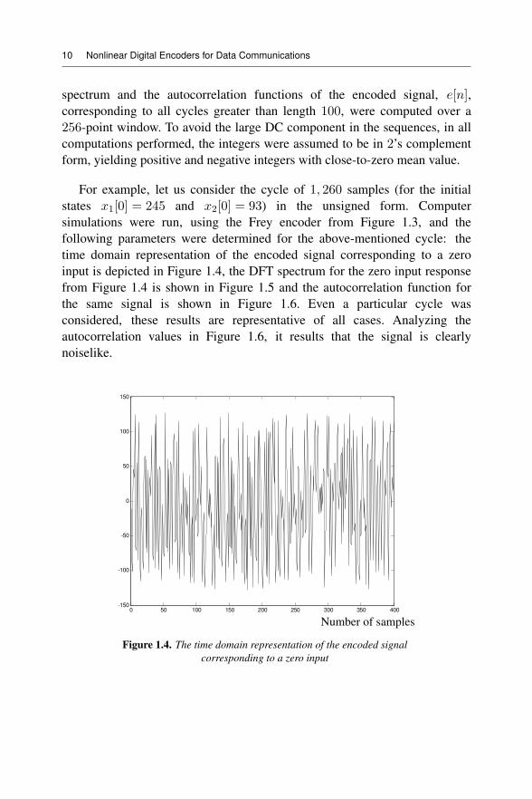
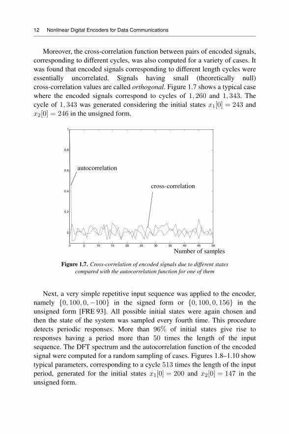
For example, let us consider the cycle of 1, 260 samples (for the initialstates x1[0] = 245 and x2[0] = 93) in the unsigned form. Computersimulations were run, using the Frey encoder from Figure 1.3, and thefollowing parameters were determined for the above-mentioned cycle: thetime domain representation of the encoded signal corresponding to a zeroinput is depicted in Figure 1.4, the DFT spectrum for the zero input responsefrom Figure 1.4 is shown in Figure 1.5 and the autocorrelation function forthe same signal is shown in Figure 1.6. Even a particular cycle wasconsidered, these results are representative of all cases. Analyzing theautocorrelation values in Figure 1.6, it results that the signal is clearlynoiselike.
0 50 100 150 200 250 300 350 400-150
-100
-50
0
50
100
150
Number of samples
Figure 1.4. The time domain representation of the encoded signalcorresponding to a zero input
Applications of Nonlinear Digital Encoders 11
50 100 150 200 2500
500
1000
1500
2000
2500
Number of samples
256-point window DFT
Figure 1.5. DFT spectrum for a zero input response
0 5 10 15 20 25 30 35 40 45 50
0
0.2
0.4
0.6
0.8
1
Number of samples
Figure 1.6. Normalized autocorrelation function for a zero input response
12 Nonlinear Digital Encoders for Data Communications
Moreover, the cross-correlation function between pairs of encoded signals,corresponding to different cycles, was also computed for a variety of cases. Itwas found that encoded signals corresponding to different length cycles wereessentially uncorrelated. Signals having small (theoretically null)cross-correlation values are called orthogonal. Figure 1.7 shows a typical casewhere the encoded signals correspond to cycles of 1, 260 and 1, 343. Thecycle of 1, 343 was generated considering the initial states x1[0] = 243 andx2[0] = 246 in the unsigned form.
0 5 10 15 20 25 30 35 40 45 50
0
0.2
0.4
0.6
0.8
1
Number of samples
autocorrelation
cross-correlation
Figure 1.7. Cross-correlation of encoded signals due to different statescompared with the autocorrelation function for one of them
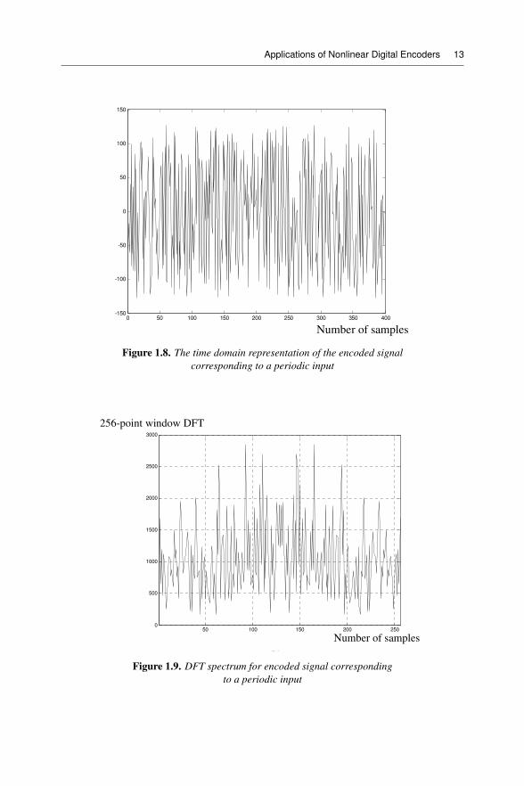
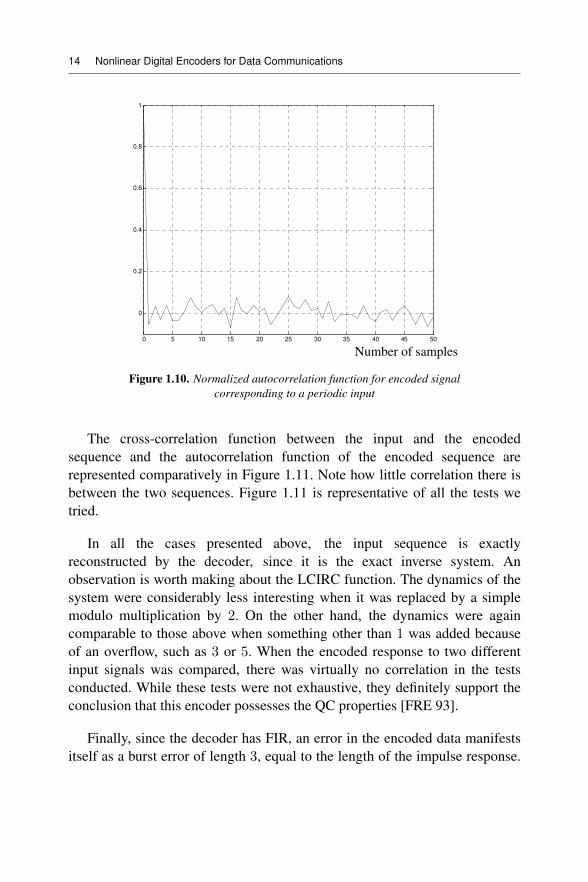
Next, a very simple repetitive input sequence was applied to the encoder,namely {0, 100, 0,−100} in the signed form or {0, 100, 0, 156} in theunsigned form [FRE 93]. All possible initial states were again chosen andthen the state of the system was sampled every fourth time. This proceduredetects periodic responses. More than 96% of initial states give rise toresponses having a period more than 50 times the length of the inputsequence. The DFT spectrum and the autocorrelation function of the encodedsignal were computed for a random sampling of cases. Figures 1.8–1.10 showtypical parameters, corresponding to a cycle 513 times the length of the inputperiod, generated for the initial states x1[0] = 200 and x2[0] = 147 in theunsigned form.
Applications of Nonlinear Digital Encoders 13
0 50 100 150 200 250 300 350 400-150
-100
-50
0
50
100
150
Number of samples
Figure 1.8. The time domain representation of the encoded signalcorresponding to a periodic input
50 100 150 200 2500
500
1000
1500
2000
2500
3000
Number of samples
(b)
256-point window DFT
Figure 1.9. DFT spectrum for encoded signal correspondingto a periodic input
14 Nonlinear Digital Encoders for Data Communications
0 5 10 15 20 25 30 35 40 45 50
0
0.2
0.4
0.6
0.8
1
Number of samples
Figure 1.10. Normalized autocorrelation function for encoded signalcorresponding to a periodic input
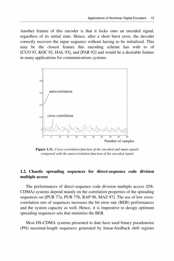
The cross-correlation function between the input and the encodedsequence and the autocorrelation function of the encoded sequence arerepresented comparatively in Figure 1.11. Note how little correlation there isbetween the two sequences. Figure 1.11 is representative of all the tests wetried.
In all the cases presented above, the input sequence is exactlyreconstructed by the decoder, since it is the exact inverse system. Anobservation is worth making about the LCIRC function. The dynamics of thesystem were considerably less interesting when it was replaced by a simplemodulo multiplication by 2. On the other hand, the dynamics were againcomparable to those above when something other than 1 was added becauseof an overflow, such as 3 or 5. When the encoded response to two differentinput signals was compared, there was virtually no correlation in the testsconducted. While these tests were not exhaustive, they definitely support theconclusion that this encoder possesses the QC properties [FRE 93].
Finally, since the decoder has FIR, an error in the encoded data manifestsitself as a burst error of length 3, equal to the length of the impulse response.
Applications of Nonlinear Digital Encoders 15
Another feature of this encoder is that it locks onto an encoded signal,regardless of its initial state. Hence, after a short burst error, the decodercorrectly recovers the input sequence without having to be initialized. Thismay be the closest feature this encoding scheme has with to of[CUO 93, KOC 92, HAL 93], and [PAR 92] and would be a desirable featurein many applications for communications systems.
0 5 10 15 20 25 30 35 40 45 50
0
0.2
0.4
0.6
0.8
1
Number of samples
autocorrelation
cross-correlation
Figure 1.11. Cross-correlation function of the encoded and input signalscompared with the autocorrelation function of the encoded signal
1.2. Chaotic spreading sequences for direct-sequence code divisionmultiple access
The performances of direct-sequence code division multiple access (DS-CDMA) systems depend mainly on the correlation properties of the spreadingsequences set [PUR 77a, PUR 77b, RAP 96, MAZ 97]. The use of low cross-correlation sets of sequences increases the bit error rate (BER) performancesand the system capacity as well. Hence, it is imperative to design optimumspreading sequences sets that minimize the BER.
Most DS-CDMA systems presented to date have used binary pseudonoise(PN) maximal-length sequences generated by linear-feedback shift register
16 Nonlinear Digital Encoders for Data Communications
(LFSR) schemes. These maximal-length sequences include Gold sequencesand Kasami sequences and proved to have quasi-orthogonality correlationproperties. Even for minimum cross-correlation sequences, forming Gold andKasami sets, the set dimension and the period of the sequences are limited bythe LFSR polynomial degree. Moreover, these sequences present values forthe cross-correlation function that depend on the generator polynomial degree[DIN 98]. Another drawback of these sequences is induced by the generatorlinearity, which increases the interception probability.
A new direct-sequence spreading method assumes the use of discrete-timenonlinear dynamical systems trajectories. These chaotic sequences presentnoiselike features that make them good for spreading in DS-CDMA systems.Unless some restrictions are specified, most chaotic systems generate almostperfect random sequences (non-periodic sequences) and their time evolution(their orbit) depends totally on the initial state of the system. So, a singlesystem, described by its discrete chaotic map, can generate a very largenumber of distinct chaotic sequences, each sequence being uniquely specifiedby its initial value [FEE 00]. This dependency on the initial state and thenonlinear character of the discrete map make the DS-CDMA system usingthese sequences more secure. Despite their general process of generation, notall the chaotic sequences are good for spreading. Like in the case of binaryPN spreading sequences, it is necessary to select the sets of chaotic PNsequences that present good correlation properties. Mazzini et al. [MAZ 97,ROV 00] proposed a new family of chaotic spreading sequences withoptimum cross-correlation properties.
To define the desired features that an optimum set of spreading sequencesmust have, we first have to present some particular details about theDS-CDMA system. Each DS-CDMA user has a unique spreading sequenceassigned to him, which has a higher data rate than the baseband signal. As amatter of fact, the baseband data signal is multiplied by the spreading signaland the resulting wideband signal acquires both the spectral and statisticalproperties of the spreading signal. Hence, all users transmit over the samewideband channel with a total overlapping in time [RAP 96]. Thismultiple-access interference (MAI) between different DS-CDMA user signalsis demonstrated to depend on the correlation properties of the spreadingsequences [PUR 77a, PUR 77b, RAP 96, MAZ 97].
Applications of Nonlinear Digital Encoders 17
Considering the fact that the DS-CDMA system performances dependmainly on the spreading sequences’ properties, we can say that an idealDS-CDMA system uses a set of optimum spreading sequences. Therefore, theoptimum set of spreading sequences is defined in the following.
DEFINITION 1.3.– The optimum set of spreading sequences for the DS-CDMAsystem is the set composed of sequences having the following properties:
1) easy to generate, by relatively simple structures;
2) to fulfill the orthogonality condition (null cross-correlation) and to havea null mean value over an information bit period;
3) to minimize the possibility to reconstruct the whole sequence from ashort fragment of it;
4) to allow an easy (and fast) sequence synchronization in the receiver;
5) to have the possibility of forming sets of sequences, which are as largeas possible, having properties 1–4.
Now, let us discuss each of the properties given above. The first propertyassures a simple implementation of the sequence generator, and therefore, italso simplifies the implementation of the DS-CDMA transmitter and receiver.As mentioned above, the orthogonality condition specified in property 2determines the reception performances for each DS-CDMA user. Hence, thesmaller the cross-correlation values for the spreading sequences, the smallerthe MAI term affecting the decision process in the receiver. The sequences’periodicity is a natural feature for all the sequences generated by a realautonomous system. Because of the numerical limitations given by theoperation with finite word lengths, the number of distinct states that such agenerator might visit is also limited to a maximum value. Therefore, thegenerated sequences are pseudo-random (almost random) and theorthogonality mentioned by property 2 depends on the period of the spreadingsequences. Also, there is an interdependence between properties 2 and 4. Inmost practical solutions, the sequence periodicity is used for realizing thesequence synchronization in the receiver, mentioned by property 4. To bemore specific, the receiver follows the periodicity of the maximumautocorrelation values in order to lock the phase of the receiver sequence. Thesecurity of the transmission scheme depends on the difficulty degree involvedin the reconstruction of the spreading sequence by an eavesdropper user.
18 Nonlinear Digital Encoders for Data Communications
Therefore, property 3 helps to increase the transmission security, because theprobability of undesired interception is reduced. Finally, property 5 refers tothe DS-CDMA system capacity, defined as the number of userssimultaneously accessing the system’s resources. Considering that each useris assigned a unique spreading sequence, the set dimension determines theDS-CDMA system capacity.
It is important to further discuss the interdependencies of properties 1 and5. For example, the use of sequences having a smaller period may ease boththeir generation (according to property 1) and synchronization (according toproperty 4), but it certainly decreases the dimension of the spreadingsequences set (according to property 5). However, increasing the sequences’period increases their randomness (according to property 2), but decreases thesynchronization performances (according to property 4). However, restrictingthe randomness properties from property 2, by introducing additionalconditions for the sequences, may determine the system capacity decrease(according to property 5), etc.
Now, it is very important to observe some similarities between the QCproperties introduced in section 1.1.2, definition 1.1, and the optimumspreading properties given in definition 1.3. The aim of this comparison is toprove that the nonlinear digital filters presented in section 1.1.3 can be usedfor DS-CDMA spreading. First, we can note that the nonlinear digital filter asshown in Figure 1.3, working in finite precision, possesses the QC propertieseven for a small word length. For example, all simulation results presented insection 1.1.4 were obtained for an 8-bit word length. Observing that thescheme as shown in Figure 1.3 presents a reduced operational complexity fora small word length, results that these filters fulfill the criterion 1 fromdefinition 1.3. However, properties 1–5 from definition 1.1 representrequirements involved in the definition of the orthogonality between thesequences, and therefore, the nonlinear filters also fulfill criterion 2 fromdefinition 1.3. Considering that the period of each sequence generated by thenonlinear digital filter in Figure 1.3 depends on the initial state of the filter,we can say that a proper selection of the initial state will allow us to select thesequences with a longer period, and therefore, criterion 3 from definition 1.3is met. However, the security provided by the Frey nonlinear digital filter wasalready demonstrated in section 1.1.4. Moreover, the high peak of theautocorrelation function of the filter’s response, provided by properties 1 and2 from definition 1.1, will certainly improve the synchronization required by
Applications of Nonlinear Digital Encoders 19
property 4 from definition 1.3. Finally, the sensitive dependency on the initialstates specified in property 5 from definition 1.1 provides the large set ofsequences required by property 5 from definition 1.3.
In conclusion, the nonlinear digital filters introduced by Frey [FRE 93] andother similar structures working in finite precision can be used both for securecommunications and for DS-CDMA spreading [ELA 06].
1.3. Sequence synchronization in discrete-time nonlinear systems
The digital chaotic communication schemes, where the chaotic signalgenerator is a discrete-time nonlinear map, allow a more reliablereconstruction of the transmitted information as compared to their analogcounterparts, due to the increased protection against noise and otherperturbations. Assuming a digital configuration with finite representation, theproblem of parameter mismatching and transmission noise surely appears lesscritical. However, as mentioned in section 1.3, the chaotic signalsynchronization from the receiver might pose some additional problems[PEC 90, KOC 92, WU 93]. Nevertheless, there are some specialdiscrete-time maps, which can exhibit the appealing property ofsynchronizing in finite time. Such a property, called “dead-beatsynchronization” as an analogy to the well-known performance ofdiscrete-time control systems [FRA 88], is applied to a simplecommunication scheme as in [TES 94, DEA 95].
1.3.1. An example of sequence synchronization using the inverse system
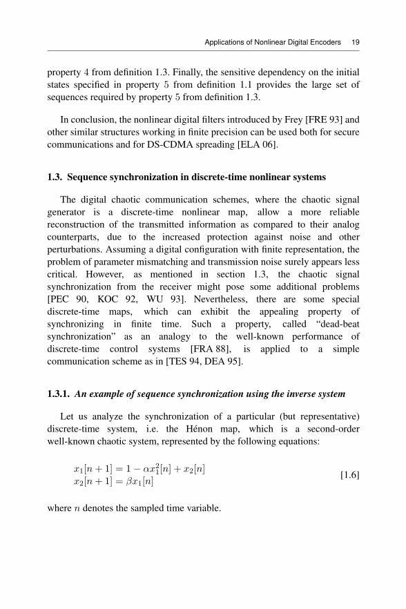
Let us analyze the synchronization of a particular (but representative)discrete-time system, i.e. the Hénon map, which is a second-orderwell-known chaotic system, represented by the following equations:
x1[n+ 1] = 1− αx21[n] + x2[n]x2[n+ 1] = βx1[n]
[1.6]
where n denotes the sampled time variable.
20 Nonlinear Digital Encoders for Data Communications
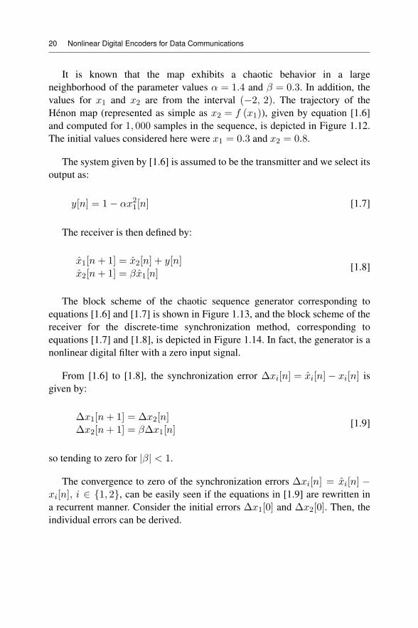
It is known that the map exhibits a chaotic behavior in a largeneighborhood of the parameter values α = 1.4 and β = 0.3. In addition, thevalues for x1 and x2 are from the interval (−2, 2). The trajectory of theHénon map (represented as simple as x2 = f (x1)), given by equation [1.6]and computed for 1, 000 samples in the sequence, is depicted in Figure 1.12.The initial values considered here were x1 = 0.3 and x2 = 0.8.
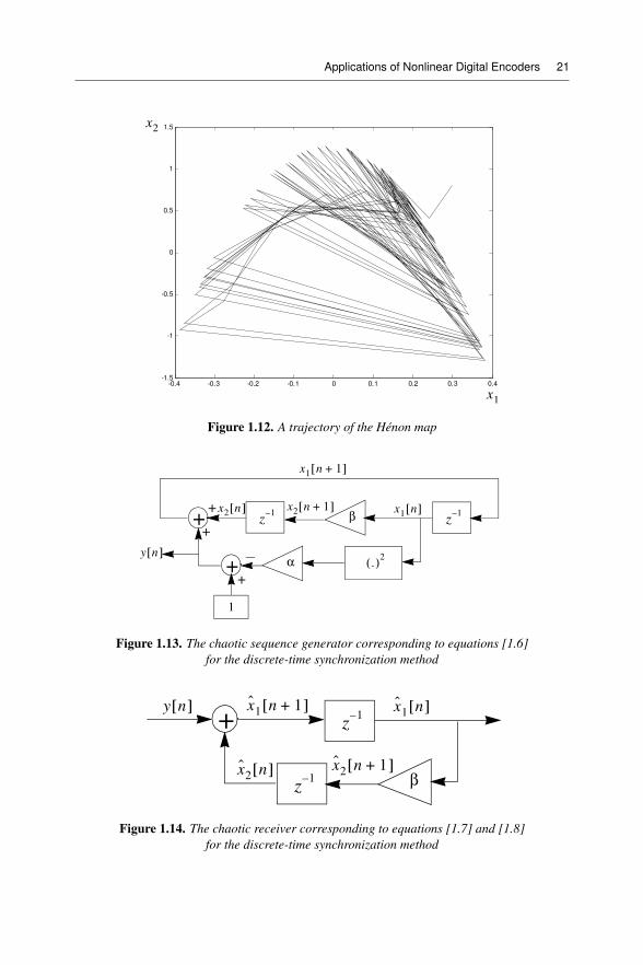
The system given by [1.6] is assumed to be the transmitter and we select itsoutput as:
y[n] = 1− αx21[n] [1.7]
The receiver is then defined by:
x1[n+ 1] = x2[n] + y[n]x2[n+ 1] = βx1[n]
[1.8]
The block scheme of the chaotic sequence generator corresponding toequations [1.6] and [1.7] is shown in Figure 1.13, and the block scheme of thereceiver for the discrete-time synchronization method, corresponding toequations [1.7] and [1.8], is depicted in Figure 1.14. In fact, the generator is anonlinear digital filter with a zero input signal.
From [1.6] to [1.8], the synchronization error Δxi[n] = xi[n]− xi[n] isgiven by:
Δx1[n+ 1] = Δx2[n]Δx2[n+ 1] = βΔx1[n]
[1.9]
so tending to zero for |β| < 1.
The convergence to zero of the synchronization errors Δxi[n] = xi[n] −xi[n], i ∈ {1, 2}, can be easily seen if the equations in [1.9] are rewritten ina recurrent manner. Consider the initial errors Δx1[0] and Δx2[0]. Then, theindividual errors can be derived.
Applications of Nonlinear Digital Encoders 21
-0.4 -0.3 -0.2 -0.1 0 0.1 0.2 0.3 0.4-1.5
-1
-0.5
0
0.5
1
1.5
x1
x2
Figure 1.12. A trajectory of the Hénon map
+
+
1
z1–
z1–β
α
+
+
+
.( )2
x1
n 1+[ ]
x1
n[ ]x2
n 1+[ ]x2
n[ ]
y n[ ]
Figure 1.13. The chaotic sequence generator corresponding to equations [1.6]for the discrete-time synchronization method
+ z1–
z1– β
x2
n 1+[ ]x2
n[ ]
y n[ ] x1
n 1+[ ] x1
n[ ]
Figure 1.14. The chaotic receiver corresponding to equations [1.7] and [1.8]for the discrete-time synchronization method
22 Nonlinear Digital Encoders for Data Communications
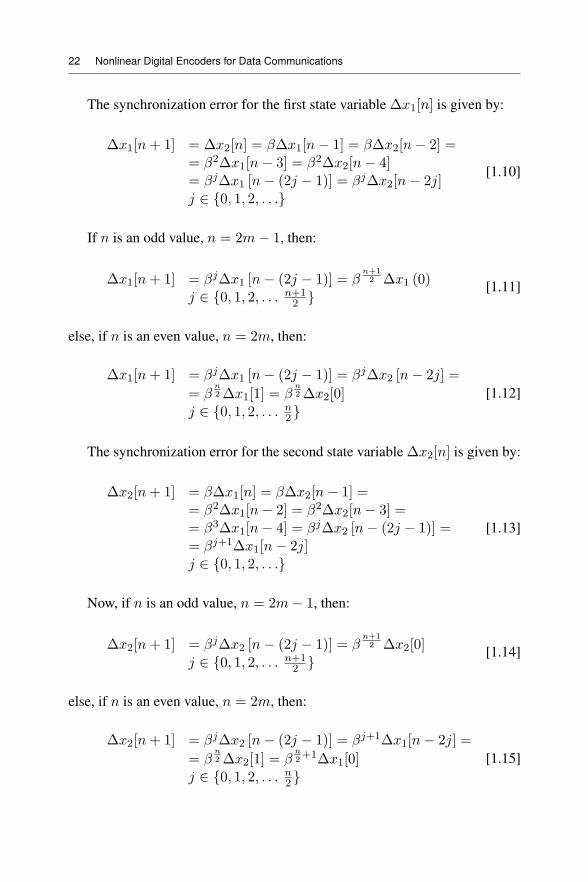
The synchronization error for the first state variable Δx1[n] is given by:
Δx1[n+ 1] = Δx2[n] = βΔx1[n− 1] = βΔx2[n− 2] == β2Δx1[n− 3] = β2Δx2[n− 4]= βjΔx1 [n− (2j − 1)] = βjΔx2[n− 2j]j ∈ {0, 1, 2, . . .}
[1.10]
If n is an odd value, n = 2m− 1, then:
Δx1[n+ 1] = βjΔx1 [n− (2j − 1)] = βn+12 Δx1 (0)
j ∈ {0, 1, 2, . . . n+12 } [1.11]
else, if n is an even value, n = 2m, then:
Δx1[n+ 1] = βjΔx1 [n− (2j − 1)] = βjΔx2 [n− 2j] =
= βn2 Δx1[1] = β
n2 Δx2[0]
j ∈ {0, 1, 2, . . . n2 }
[1.12]
The synchronization error for the second state variable Δx2[n] is given by:
Δx2[n+ 1] = βΔx1[n] = βΔx2[n− 1] == β2Δx1[n− 2] = β2Δx2[n− 3] == β3Δx1[n− 4] = βjΔx2 [n− (2j − 1)] == βj+1Δx1[n− 2j]j ∈ {0, 1, 2, . . .}
[1.13]
Now, if n is an odd value, n = 2m− 1, then:
Δx2[n+ 1] = βjΔx2 [n− (2j − 1)] = βn+12 Δx2[0]
j ∈ {0, 1, 2, . . . n+12 } [1.14]
else, if n is an even value, n = 2m, then:
Δx2[n+ 1] = βjΔx2 [n− (2j − 1)] = βj+1Δx1[n− 2j] =
= βn2 Δx2[1] = β
n2+1Δx1[0]
j ∈ {0, 1, 2, . . . n2 }
[1.15]
Applications of Nonlinear Digital Encoders 23
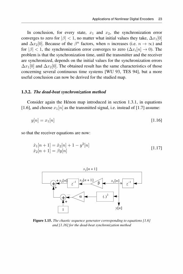
In conclusion, for every state, x1 and x2, the synchronization errorconverges to zero for |β| < 1, no matter what initial values they take, Δx1[0]and Δx2[0]. Because of the βn factors, when n increases (i.e. n → ∞) andfor |β| < 1, the synchronization error converges to zero (Δxi[n] → 0). Theproblem is that the synchronization time, until the transmitter and the receiverare synchronized, depends on the initial values for the synchronization errorsΔx1[0] and Δx2[0]. The obtained result has the same characteristics of thoseconcerning several continuous time systems [WU 93, TES 94], but a moreuseful conclusion can now be derived for the studied map.
1.3.2. The dead-beat synchronization method
Consider again the Hénon map introduced in section 1.3.1, in equations[1.6], and choose x1[n] as the transmitted signal, i.e. instead of [1.7] assume:
y[n] = x1[n] [1.16]
so that the receiver equations are now:
x1[n+ 1] = x2[n] + 1− y2[n]x2[n+ 1] = βy[n]
[1.17]
+
+
1
z1–
z1–β
α
+
+
+
.( )2
x1
n 1+[ ]
x1
n[ ]x2
n 1+[ ]x2
n[ ]
y n[ ]
x
Figure 1.15. The chaotic sequence generator corresponding to equations [1.6]and [1.16] for the dead-beat synchronization method
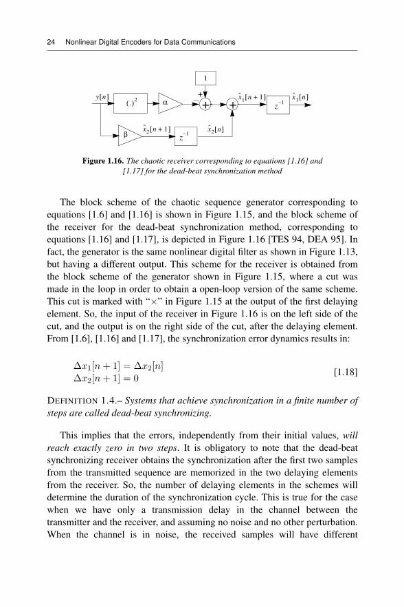
24 Nonlinear Digital Encoders for Data Communications
+ z1–
z1–β
x2
n 1+[ ] x2
n[ ]
y n[ ] x1
n 1+[ ] x1
n[ ]
+
1
α
+
.( )2
Figure 1.16. The chaotic receiver corresponding to equations [1.16] and[1.17] for the dead-beat synchronization method
The block scheme of the chaotic sequence generator corresponding toequations [1.6] and [1.16] is shown in Figure 1.15, and the block scheme ofthe receiver for the dead-beat synchronization method, corresponding toequations [1.16] and [1.17], is depicted in Figure 1.16 [TES 94, DEA 95]. Infact, the generator is the same nonlinear digital filter as shown in Figure 1.13,but having a different output. This scheme for the receiver is obtained fromthe block scheme of the generator shown in Figure 1.15, where a cut wasmade in the loop in order to obtain a open-loop version of the same scheme.This cut is marked with “×” in Figure 1.15 at the output of the first delayingelement. So, the input of the receiver in Figure 1.16 is on the left side of thecut, and the output is on the right side of the cut, after the delaying element.From [1.6], [1.16] and [1.17], the synchronization error dynamics results in:
Δx1[n+ 1] = Δx2[n]Δx2[n+ 1] = 0
[1.18]
DEFINITION 1.4.– Systems that achieve synchronization in a finite number ofsteps are called dead-beat synchronizing.
This implies that the errors, independently from their initial values, willreach exactly zero in two steps. It is obligatory to note that the dead-beatsynchronizing receiver obtains the synchronization after the first two samplesfrom the transmitted sequence are memorized in the two delaying elementsfrom the receiver. So, the number of delaying elements in the schemes willdetermine the duration of the synchronization cycle. This is true for the casewhen we have only a transmission delay in the channel between thetransmitter and the receiver, and assuming no noise and no other perturbation.When the channel is in noise, the received samples will have different
Applications of Nonlinear Digital Encoders 25
amplitudes, so the signal at the output of the receiver will synchronize withthe received sequence, instead of the transmitted sequence. This is why areduction method for the noise effects is needed in the receiver to improve thesynchronization. For this case with noise, the synchronization cycle willexceed the duration of two steps, as before. A method for reducing the noiseeffects in the dead-beat synchronizing receiver is presented in [DE 95].
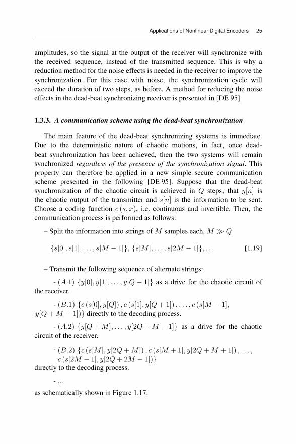
1.3.3. A communication scheme using the dead-beat synchronization
The main feature of the dead-beat synchronizing systems is immediate.Due to the deterministic nature of chaotic motions, in fact, once dead-beat synchronization has been achieved, then the two systems will remainsynchronized regardless of the presence of the synchronization signal. Thisproperty can therefore be applied in a new simple secure communicationscheme presented in the following [DE 95]. Suppose that the dead-beatsynchronization of the chaotic circuit is achieved in Q steps, that y[n] isthe chaotic output of the transmitter and s[n] is the information to be sent.Choose a coding function c (s, x), i.e. continuous and invertible. Then, thecommunication process is performed as follows:
– Split the information into strings of M samples each, M Q
{s[0], s[1], . . . , s[M − 1]}, {s[M ], . . . , s[2M − 1]}, . . . [1.19]
– Transmit the following sequence of alternate strings:
- (A.1) {y[0], y[1], . . . , y[Q− 1]} as a drive for the chaotic circuit ofthe receiver.
- (B.1) {c (s[0], y[Q]) , c (s[1], y[Q+ 1]) , . . . , c (s[M − 1],y[Q+M − 1])} directly to the decoding process.
- (A.2) {y[Q+M ], . . . , y[2Q+M − 1]} as a drive for the chaoticcircuit of the receiver.
- (B.2) {c (s[M ], y[2Q+M ]) , c (s[M + 1], y[2Q+M + 1]) , . . . ,c (s[2M − 1], y[2Q+ 2M − 1])}
directly to the decoding process.
- ...
as schematically shown in Figure 1.17.
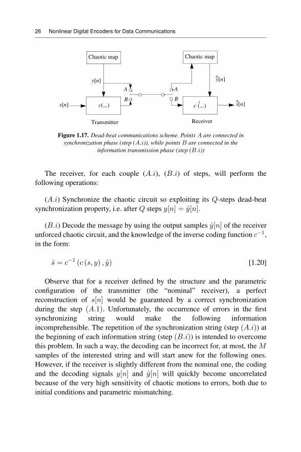
26 Nonlinear Digital Encoders for Data Communications
Chaotic map
c(.,.)
Chaotic map
c (.,.)1–
Transmitter Receiver
y[n]
s[n]
y[n]^
s[n]^
A
B
A
B
Figure 1.17. Dead-beat communications scheme. Points A are connected insynchronization phase (step (A.i)), while points B are connected in the
information transmission phase (step (B.i))
The receiver, for each couple (A.i), (B.i) of steps, will perform thefollowing operations:
(A.i) Synchronize the chaotic circuit so exploiting its Q-steps dead-beatsynchronization property, i.e. after Q steps y[n] = y[n].
(B.i) Decode the message by using the output samples y[n] of the receiverunforced chaotic circuit, and the knowledge of the inverse coding function c−1,in the form:
s = c−1 (c (s, y) , y) [1.20]
Observe that for a receiver defined by the structure and the parametricconfiguration of the transmitter (the “nominal” receiver), a perfectreconstruction of s[n] would be guaranteed by a correct synchronizationduring the step (A.1). Unfortunately, the occurrence of errors in the firstsynchronizing string would make the following informationincomprehensible. The repetition of the synchronization string (step (A.i)) atthe beginning of each information string (step (B.i)) is intended to overcomethis problem. In such a way, the decoding can be incorrect for, at most, the Msamples of the interested string and will start anew for the following ones.However, if the receiver is slightly different from the nominal one, the codingand the decoding signals y[n] and y[n] will quickly become uncorrelatedbecause of the very high sensitivity of chaotic motions to errors, both due toinitial conditions and parametric mismatching.
Applications of Nonlinear Digital Encoders 27
It is important to note that after each synchronization step (A.i), theopen-loop receiver must be changed to a closed-loop scheme, such as thetransmitter shown in Figure 1.15. During the information transmission step(B.i), the receiver must work as a stand-alone, independent system, so thatthe transmitter does. Hence, when the switches in the transmitter and thereceiver change their positions from A to B, at the same time, the receiverblock must switch from the open-loop mode to the closed-loop mode, byre-establishing the connection cut and marked by “×” as shown inFigure 1.15.

2
Presentation of the Frey NonlinearEncoder as a Digital Filter
2.1. The mathematical analysis of the Frey encoder
In this section, the Frey encoder presented in section 1.1.3 is analyzed. Thisprovides some insight into the properties observed earlier in sections 1.1.3 and1.1.4. This analysis is possible because of the special properties of the modulooperator, as used in [FRE 93, CHU 88, CHU 90] and [EBE 69]. First, let usreconsider the encoder-defining equations [1.3], resulting from the scheme inFigure 1.3, where this time the modulo operator is explicitly written as follows:
e[n] = mod (u[n] +mod[x1[n] + x2[n]])= mod (u[n] + x1[n] + x2[n])
x1[n] = e[n− 1]x2[n] = LCIRC (x1[n− 1])
= mod (2x1[n− 1] + s[n])
s[n] =0 if x1[n− 1] < 2N−1
1 otherwise
[2.1]
where N is the binary word length, x1[n] = x[n− 1] and x2[n] = x[n− 2] arethe states, namely the outputs of the delays, and the modulo operator has thebase given by 2N . Also, the expression of the left-circulate (LCIRC) function,introduced in definition 1.2, has been used here. Combining these equations,
30 Nonlinear Digital Encoders for Data Communications
we have:
e[n] = mod (u[n] + e[n− 1] +mod (2e (n− 2) + s[n]))= mod (u[n] + e[n− 1] + 2e[n− 2] + s[n])
[2.2]
Note that s[n] plays the role of a noise source that is correlated in anonlinear way to the response, e[n].
In [PEN 01], Penaud thoroughly analyzed the recursive system used byFrey to generate the chaotic sequences. In fact, Penaud introduced a moregeneral case of the coder/decoder scheme proposed by Frey in [FRE 93].Hence, equations [2.1] and [2.2] are rewritten in a generalized form asfollows:
e[n] = u[n]⊕ fM
i=1
(Kie [n−Di]⊕ s [n]) [2.3]
where f (x) =x if −2N−1 ≤ x ≤ 2N−1 − 1xmod 2N otherwise
. In all the computations
performed, the integer values for e [n], u [n], s [n] and Ki were assumed tobe represented in 2’s complement form (C2), yielding positive and negativeintegers with a mean value close to zero. Also, all additions are modulo-2N ,where N is the binary equivalent word length. These operators are assumed tobe generally nonlinear operations, due to overflow in the actual finite lengthadders used for hardware computation.
It can be easily seen that the basic Frey codec presented in section 1.1.3(equation [1.3]) is a particular case of the system given by [2.3], consideringM = 2, K1 = 1, K2 = 2, D1 = 1 and D2 = 2, respectively.
The detailed expressions for the definitions and properties of theseoperators are presented in section 2.2.
2.2. The definitions and properties of the unsigned and 2’s complementsigned sample operators
DEFINITION 2.1.– An unsigned number, denoted as yU , is a natural numberrepresented with code words of N bits. From this point on, the superscript Uwill denote an unsigned number, which is a positive integer.
Presentation of the Frey Nonlinear Encoder as a Digital Filter 31
If the following notation is considered, i.e. yU = xUmod 2N , thenyU ∈ 0, 2N − 1 , for any positive integer number xU . If xU is already avalue less than 2N − 1, then we have the following expression:yU = xU = xUmod 2N ∈ 0, 2N − 1 .
DEFINITION 2.2.– An signed number, denoted as ys, is an integer number,represented in 2’s complement (C2) form with code words of N bits. From thispoint on, the superscript s will denote a signed C2 number, which is an integer.
If the following notation is considered, i.e. yS = xSmod 2N , thenyS ∈ −2N−1, 2N − 1 , for any signed integer number xS . If xS is already avalue from the modulo C2 interval, i.e. xS ∈ −2N−1, 2N − 1 , then yS iscomputed as follows: yS = xS = xSmod 2N ∈ −2N−1, 2N−1 − 1 . Inthe sequel, we will show how this signed number is expressed.
DEFINITION 2.3.– The two sets of integer numbers presented above,xU ∈ {0, 2N − 1} and xS ∈ −2N−1, 2N−1 − 1 , will be referred to as the2N -set and the C2, 2N -set, respectively.
DEFINITION 2.4.– The number xU is converted into its corresponding signedC2 value, xS , using the following equation:
xUS
= xS
=xU if 0 ≤ xU ≤ 2N−1 − 1C2 2N − xU = xU − 2N if 2N−1 ≤ xU ≤ 2N − 1
[2.4]
where C2 (x) is the 2’s complement value for x represented with N bits.
In the following, this operation will be denoted as xUS and is defined as
the conversion function from the unsigned natural representation to thesigned 2’s complement representation: xU
S= xS , where
xS ∈ −2N−1, 2N−1 − 1 and xU ∈ 0, 2N − 1 .
NOTE 2.1.– For the general case, when the unsigned natural number xU doesnot necessarily take a value from the interval xU ∈ 0, 2N − 1 , theconversion from the unsigned form to the signed C2 form can be performedas follows:
yS = xSmod 2N = xUmod 2NS
[2.5]
32 Nonlinear Digital Encoders for Data Communications
In fact, a new operator was used, the signed modulo-2N operator. Thisoperation consists of computing the normal modulo-2N value and then, aconversion to the signed C2 form is performed, as above. The aboveexpression is used to estimate any signed number, as defined in definition 2.2.
DEFINITION 2.5.– The inverse operation of xUS , which performs the
conversion function from the signed 2’s complement representation to theunsigned natural representation, is denoted by xS
U . The number xS isconverted into its corresponding unsigned value, xU , as follows:
xU =xS if 0 ≤ xS ≤ 2N−1 − 1xS + 2N if −2N−1 ≤ xS < 0
[2.6]
where xSU= xU , xS ∈ −2N−1, 2N−1 − 1 and xU ∈ 0, 2N − 1 .
DEFINITION 2.6.– The addition operator of unsigned xU numbers in the2N -set. Let us consider two unsigned numbers xU , yU ∈ 0, 2N − 1 , thenwe define the addition operation in the 2N -set as:
zU = xU ⊕ yU = xU + yU mod 2N
zU ∈ 0, 2N − 1[2.7]
NOTE 2.2.– Because of some properties of the modulo-2N operation, we canderive some new expressions.
In the general case, for the expression amod b, we have:
amod b = r [2.8]
where r is the remainder of the division of a and b ab :
a = bc+ r [2.9]
and c is the quotient of ab .
Presentation of the Frey Nonlinear Encoder as a Digital Filter 33
For the case discussed above, when we use the modulo-2N operation forthe unsigned 2N -set numbers, we can write:
xU + yU mod 2N = r ⇔ xU + yU = 2Nc+ r [2.10]
When xU , yU ∈ 0, 2N − 1 , we have 0 ≤ xU + yU ≤ 2N+1 − 2, andthen the quote c takes one of the values c in{0, 1}. Taking this into account,the next expression can be derived:
xU + yU =2N + xU + yU mod 2N if c = 1xU + yU mod 2N if c = 0
[2.11]
Equation [2.11] is equivalent to:
xU + yU =
⎧⎪⎪⎨⎪⎪⎩2N + xU + yU mod 2N
if 2N ≤ xU + yU ≤ 2N+1 − 2xU + yU mod 2N
if 0 ≤ xU + yU ≤ 2N − 1
[2.12]
Now, from equations [2.11] and [2.12], the following expression for theaddition operation in the 2N -set is obtained:
r = zU = xU ⊕ yU =
=xU + yU − 2N if 2N ≤ xU + yU ≤ 2N+1 − 2xU + yU if 0 ≤ xU + yU ≤ 2N − 1
zU ∈ 0, 2N − 1
[2.13]
NOTE 2.3.– In the following, we can note that the condition0 ≤ xU + yU ≤ 2N+1 − 2 is equivalent to 0 ≤ 2Nc+ r ≤ 2N+1 − 2.Therefore, considering equations [2.8] and [2.9], we have two possiblecases:
1) If c = 0 ⇒ 0 ≤ r ≤ 2N − 1, or
2) If c = 1 ⇒ 0 ≤ 2N + r ≤ 2N+1 − 2.
34 Nonlinear Digital Encoders for Data Communications
So, considering both cases, the remainder r can take a value only fromthe reunion interval: r = zU ∈ { 0, 2N − 1 ∪ 0, 2N − 2 } = 0, 2N − 1 .Hence, the condition zU ∈ 0, 2N − 1 from [2.13] is obvious.
NOTE 2.4.– Taking into account the previous observation and equation [2.13],a general expression of the addition operation, for any number of terms, in the2N -set can be derived. Let us consider m unsigned valuesai
U , i ∈ [1, m] , aiU ∈ 0, 2N − 1 . In the appendix, it is demonstrated that
the addition of all these values, in the 2N -set, is given by the followingequation:
bU = a1U ⊕ a2
U ⊕ a3U ⊕ . . .⊕ am
U =m
i=1ai
U mod 2N =⎧⎪⎪⎪⎪⎪⎪⎪⎪⎪⎪⎪⎪⎪⎪⎪⎪⎪⎪⎪⎪⎪⎪⎪⎨⎪⎪⎪⎪⎪⎪⎪⎪⎪⎪⎪⎪⎪⎪⎪⎪⎪⎪⎪⎪⎪⎪⎪⎩
m
i=1ai
U − (m− 1) 2N
if (m− 1) 2N ≤m
i=1ai
U ≤ m2N −m
m
i=1ai
U − (m− 2) 2N
if (m− 2) 2N ≤m
i=1ai
U ≤ (m− 1) 2N − 1
m
i=1ai
U − (m− 3) 2N
if (m− 3) 2N ≤m
i=1ai
U ≤ (m− 2) 2N − 1
. . . . . . . . . . . . . . .m
i=1ai
U if 0 ≤m
i=1ai
U ≤ 2N − 1
bU ∈ 0, 2N − 1
[2.14]
DEFINITION 2.7.– The addition operator of signed xS numbers in theC2, 2N -set. Let us consider two signed C2 numbersxS , yS ∈ −2N−1, 2N−1 − 1 , then we define the addition operation in theC2, 2N -set as:
zS = xS ⊕ yS = xU ⊕ yUS= xU + yU mod 2N
S= zU
S
zS = zUS ∈ −2N−1, 2N − 1
[2.15]
Presentation of the Frey Nonlinear Encoder as a Digital Filter 35
THEOREM 2.1.– The addition operation in the C2, 2N -set is associative.
This associativity property can be expressed as follows:
xS ⊕ yS ⊕ zS = xS ⊕ yS ⊕ zS = xS ⊕ yS ⊕ zS
xS , yS , zS ∈ −2N−1, 2N − 1[2.16]
DEMONSTRATION 2.1.– According to definition 2.7 and [2.11], we can derivethe following:
xS ⊕ yS = xU ⊕ yUS
[2.17]
and then:
xS ⊕ yS ⊕ zS = xU ⊕ yU ⊕ zUS
[2.18]
q.e.d.
NOTE 2.5.– If the addition operation in the 2N -set is associative, then theaddition operation in C2, 2N -set is also associative.
THEOREM 2.2.– The addition operation in the 2N -set is associative:
wU = xU ⊕ yU ⊕ zU = xU ⊕ yU ⊕ zU = xU ⊕ yU ⊕ zU == xU + yU + zU mod 2N
wU ∈ 0, 2N − 1[2.19]
The demonstration of theorem 2.2 is presented in the appendix.
THEOREM 2.3.– The addition operation in the C2, 2N -set is commutative.This commutativity property can be expressed as follows:
xS ⊕ yS = yS ⊕ xS
xS , yS ∈ −2N−1, 2N−1 − 1[2.20]
36 Nonlinear Digital Encoders for Data Communications
DEMONSTRATION 2.2.– According to equations [2.7] and [2.13] indefinition 2.6 and taking into account the commutativity property of theaddition operation for integer values, it is obvious that the addition operationin the 2N -set is also commutative. Now, from equation [2.15] indefinition 2.7, it results that the addition operation in the C2, 2N -set is alsocommutative.
q.e.d.
DEFINITION 2.8.– The subtraction operator of unsigned numbers in the2N -set. Let us consider two unsigned numbers yU , zU ∈ 0, 2N − 1 , thenwe define the subtraction operation in the 2N -set as:
xU = zU yU = zU − yU mod 2N
xU , yU , zU ∈ 0, 2N − 1[2.21]
THEOREM 2.4.– The subtraction operator of unsigned numbers in the 2N -setis the inverse of the addition operator of unsigned numbers in the 2N -set. Inanother words, if zU = xU ⊕ yU , then xU = zU yU and vice versa.
The demonstration of theorem 2.4 is presented in the appendix.
NOTE 2.6.– From equation [2.21] and similarly to equation [2.13], thefollowing compact expression for the operator is obtained:
xU = zU yU =zU − yU + 2N if −2N + 1 ≤ zU − yU ≤ −1zU − yU if 0 ≤ zU − yU ≤ 2N − 1
xU , yU , zU ∈ 0, 2N − 1[2.22]
DEFINITION 2.9.– The subtraction operator of signed xS numbers in theC2, 2N -set. Similar to equation [2.15] in definition 2.7, we can define a
subtraction operator of signed xS numbers in the C2, 2N -set. Let usconsider two signed C2 numbers xS , yS ∈ −2N−1, 2N−1 − 1 , then wedefine the subtraction operation in the C2, 2N -set as:
xS = zS yS = zU yUS= zU − yU mod 2N
S= xU
S
xS = xUS ∈ −2N−1, 2N−1 − 1
[2.23]
Presentation of the Frey Nonlinear Encoder as a Digital Filter 37
NOTE 2.7.– The subtraction operator of signed xS numbers in the C2, 2N -setwas used to define the chaotic decoders in [FRE 93] and [PEN 01].
NOTE 2.8.– The subtraction operator represents the reverse operation for theaddition operation in the C2, 2N -set.
DEFINITION 2.10.– The multiplication operator of unsigned xU numbers inthe 2N -set. Let us consider two unsigned numbers xU , yU ∈ 0, 2N − 1 , thenwe define the multiplication operation in the 2N -set as:
zU = xU ⊗ yU = xU · yU mod 2N
xU , yU , zU ∈ 0, 2N − 1[2.24]
NOTE 2.9.– From equation [2.24] and similarly to [2.13], the followingexpression for the ⊗ operator is obtained:
zU = xU ⊗ yU
=
⎧⎪⎪⎪⎪⎪⎪⎪⎪⎪⎪⎨⎪⎪⎪⎪⎪⎪⎪⎪⎪⎪⎩
xU · yU − 2N − 2 2N
if 2N − 2 2N ≤ xU · yU ≤ 2N − 2 2N + 1xU · yU − 2N − 3 2N
if 2N − 3 2N ≤ xU · yU ≤ 2N − 2 2N − 1. . . . . . . . . . . . . . .xU · yU − 2 · 2N if 2 · 2N ≤ xU · yU ≤ 3 · 2N − 1xU · yU − 2N if 2N ≤ xU · yU ≤ 2 · 2N − 1xU · yU if 0 ≤ xU · yU ≤ 2N − 1
xU , yU , zU ∈ 0, 2N − 1 [2.25]
DEFINITION 2.11.– The multiplication operator of signed numbers in theC2, 2N -set. Similar to equation [2.15] in definition 2.7, we can define a
multiplication operator of signed xS numbers in the C2, 2N -set. Let usconsider two signed C2 numbers xS , yS ∈ −2N−1, 2N−1 − 1 , then we
38 Nonlinear Digital Encoders for Data Communications
define the multiplication operation in the C2, 2N -set as:
zS = xS ⊗ yS = xU ⊗ yUS= xU · yU mod 2N
S= zU
S
zS = zUS ∈ −2N−1, 2N−1 − 1
[2.26]
2.3. The properties of the LCIRC nonlinear function used in the Freyencoder scheme
In section 1.1.3, it was mentioned that Frey proposed a 2’s complementrepresentation form for all the computations in the codec in Figure 1.3, in orderto determine a direct current (DC) component close to zero. To simplify thecodec analysis, we will consider a conversion from the signed 2’s complementform to the unsigned form and its reverse conversion. Therefore, the codec inFigure 1.3 that works entirely in signed 2’s complement can be changed to anequivalent codec that first converts each signed input sample value uS [n] intoan unsigned value uU [n], processes it in unsigned modulo-2N form and then atthe output, converts each unsigned input eU [n] sample value into a signed valueeS [n]. For this scheme equivalency, we used the operators and their propertiesintroduced in section 2.2. This equivalent scheme was used for all simulationsin sections 1.1.4 and 2.4. More details about this simulation scheme are alsopresented in section 2.4.
In the following, some properties of the LCIRC function are analyzed.
Using definition 2.6 for the addition operator of unsigned xU numbers inthe 2N -set (equation [2.7]), expression [1.4] can be rewritten as:
yU = 2 · xU ⊕ sxU , yU ∈ 0, 2N − 1
[2.27]
where the time variable n was eliminated for the sake of clarity.
NOTE 2.10.– The unsigned natural value for the product 2 · xU from equation[2.27] does not necessarily take a value from the interval 0, 2N − 1 . Onlythe unsigned natural number xU is from the interval xU ∈ 0, 2N − 1 . Also,the unsigned natural value s takes a value from two: 0 or 1, both being fromthe interval 0, 2N − 1 . So, we can consider s as an unsigned number in the
Presentation of the Frey Nonlinear Encoder as a Digital Filter 39
2N -set, s = sU . In fact, s adds a value 1 to the product 2 · xU only if thisproduct exceeds the 2N -set interval’s maximum limit. This feature confers thenonlinear property of this function.
THEOREM 2.5.– If unsigned number xU from the 2N -set is represented in abinary string, from the 2N -field (2-base) form, asx(2)
U = (xN−1, xN−2, . . . , x1, x0), where {xi, i ∈ {0, . . . N − 1}} = {0, 1},and the 10-base representation of x(2) is:
xU = xU(10) = xN−1 · 2N−1 + xN−2 · 2N−2 + . . .+ x1 · 2 + x0
=N−1
i=1
xi · 2i, [2.28]
then the LCIRC value of xU is having the binary representation as:
yU = y(10)U = LCIRC xU
⇒ y(2)U = (xN−2, xN−3, . . . , x1, x0, xN−1) [2.29]
NOTE 2.11.– From [2.29], it is obvious that in the binary representation ofy(2), the first bit, i.e. the most significant bit (MSB), from x(2) has changed itsposition to the least significant bit (LSB) position, and all the other bits in x(2)have been shifted one position to the left. This is the reason for calling thisfunction the LCIRC function.
DEMONSTRATION 2.3.– Let us consider the following notations for thebinary representations of yU and xU as y(2)
U = (yN−1, yN−2, . . . , y1, y0),and x(2)
U = (xN−1, xN−2, . . . , x1, x0), respectively. Then, regarding thevalue of the MSB in x(2)
U , we have two possible cases:
Case (a) xN−1 = 0. In this case, the decimal value of xU is within theinterval 0 ≤ x(10)
U ≤ 2N−1 − 1 ⇒ s = 0 and then 0 ≤ 2 · x(10)U ≤ 2N − 2.Now, the decimal value for yU can be expressed as:y(10)
U = LCIRC x(10)U = 2 · x(10)U + s mod 2N = 2x(10)
U . Usingthe binary representation for xU , and considering xN−1 = 0, the nextexpression is derived:
y(10)U= 2x(10)
U = 2 · xN−1 · 2N−1 + xN−2 · 2N−2 + . . .+ x1 · 2 + x0= xN−2 · 2N−1 + xN−3 · 2N−2 + . . .+ x1 · 22 + x0 · 2 + 0 · 20 .
40 Nonlinear Digital Encoders for Data Communications
Considering the LSB as xN−1 = 0, the binary representation for yU isgiven by:
y(2)U = (xN−2, xN−3, . . . , x1, x0, xN−1) [2.30]
q.e.d.
Case (b) xN−1 = 1. In this case, the decimal value of xU is within theinterval: 2N−1 ≤ x(10)
U ≤ 2N − 1 ⇒ s = 1 and then 2N ≤ 2 · x(10)U≤ 2N+1 − 2. The argument for the LCIRC function respects the condition:2N +1 ≤ 2 · x(10)U + s ≤ 2N+1 − 1. Now, from the definition of the additionoperation in the 2N -set (equation [2.13]), the decimal value for yU can beexpressed as: y(10)
U = LCIRC x(10)U = 2 · x(10)U + 1 mod 2N =
2x(10)U + 1 − 2N . Using the binary representation for xU , and considering
xN−1 = 1, the next expression is derived:
y(10)U= 2x(10)
U + 1− 2N
= 2 · xN−1 · 2N−1 + xN−2 · 2N−2 + . . .+ x1 · 2 + x0 + 1− 2N
= 2N + xN−2 · 2N−1 + xN−3 · 2N−2 + . . .+ x1 · 22 + x0 · 2+1− 2N
= xN−2 · 2N−1 + xN−3 · 2N−2 + . . .+ x1 · 22 + x0 · 2 + 1 · 20.
Considering the LSB as xN−1 = 1, the binary representation for yU isgiven by:
y(2)U = (xN−2, xN−3, . . . , x1, x0, xN−1) [2.31]
q.e.d.
Considering both the cases, a and b, theorem 2.5 is demonstrated.
The LCIRC shifting of one position to the left in the binary representationof the argument demonstrated in theorem 2.5 can be generalized for anynumber of bit rotations. This general LCIRC function is defined in thefollowing.
DEFINITION 2.12.– Considering a bit index denoted by k for the binaryrepresentations using N bits in a code word, the LCIRC function application
Presentation of the Frey Nonlinear Encoder as a Digital Filter 41
for k times consecutively is defined as follows:
LCIRCk xU LCIRC LCIRC . . . LCIRC xU
k times[2.32]
THEOREM 2.6.– The LCIRC function application for k times, defined in[2.32], determines a k bits rotation in the binary code word.
The demonstration of theorem 2.6 is similar to the demonstration given fortheorem 2.5, considering the latter in each bit rotation from the k rotations.
NOTE 2.12.– As a result of theorem 2.6, when applying, for N timesconsecutively, the LCIRC function to an N bits word length unsigned valuexU , it results in the original argument value:
LCIRCN xU LCIRC LCIRC . . . LCIRC xU = xU
N times[2.33]
2.4. The simulation of the Frey sequence generator block in Simulink:some practical considerations
2.4.1. The transmitter chaotic sequence generator
Considering the properties of the operators defined in sections 2.2 and 2.3for signed xS numbers in the C2, 2N -set and using the block scheme of thebasic encoder–decoder proposed by Frey in [FRE 93] and shown in Figure 1.3(section 1.1.3), a chaotic sequence generator was implemented in Simulink.
The signal at the output of this generator is composed by the Bi quantifiedlevels, represented with N bits word length and having the duration of Tseconds, for each output sample. The extreme quantified levels, determinedby the word length N , take the values:
L = −2N−1, Lmax = 2N−1−1.
42 Nonlinear Digital Encoders for Data Communications
To reduce the signal’s power and not to make its amplitude depend on thenumber of levels (in fact, on N ), all the levels are normalized by the maximumabsolute value of the quantified levels, L = 2N−1. Then, the generated chaoticsignal is given by:
e S (t) =∞
i=0
BipT (t− iT ) [2.34]
where −2N−1
L ≤ Bi ≤ 2N−1−1L , L = 2N−1 ⇒ −1 ≤ Bi ≤ 1
and pT (t) =1 if 0 ≤ t ≤ T0 otherwise
The input signal of the encoder will be used as a key signal to change thegenerator’s dynamics. The block scheme used to simulate the chaotic signalgenerator is shown in Figure 2.1.
As discussed in section 1.1.3, this block scheme includes two delayelements and some modulo-2N adders. To benefit from the modulo functiondefined for real, positive numbers, some conversions from the unsigned xU
number representation in the 2N -set to signed xS number representation inthe C2, 2N -set, and the reverse conversion, were performed. Theseconversions follow equations [2.4] and [2.5], presented in section 2.2. Hence,the idea was to make the loop work in the unsigned manner inside, and tooutput the signal in a signed manner. The output signal e S [n] is thenormalized signed representation signal obtained from the internal unsignedrepresentation sequence eU [n]. This normalized signal will be used fortransmission. The signal eU [n] is passed through two consecutive delayelements, in the unsigned internal representation, and added modulo-2N
according to the basic encoder scheme shown in Figure 1.3 (section 1.1.3).Before the normalization, the signal is converted to the signed form.
The block denoted as “carry bit function s[n]”, represents a block thatverifies the condition for adding the carry bit and performs this additioncorrespondingly, according to definition 1.2 of LCIRC, presented insection 1.1.3. The signal s[n] generated like this was considered as a sequenceof unsigned 2N -set values and the addition operation with the double value ofeU [n− 2] was considered as a modulo-2N addition. According to the
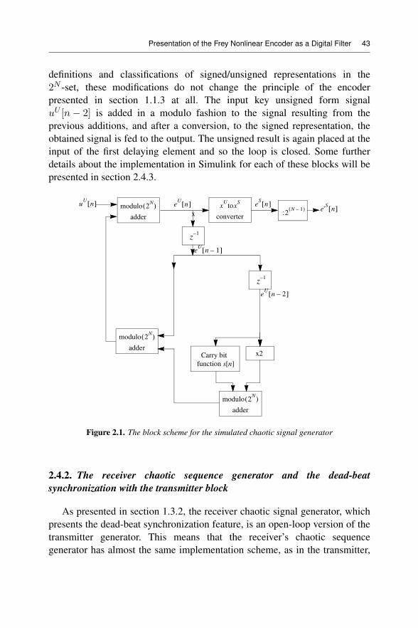
Presentation of the Frey Nonlinear Encoder as a Digital Filter 43
definitions and classifications of signed/unsigned representations in the2N -set, these modifications do not change the principle of the encoderpresented in section 1.1.3 at all. The input key unsigned form signaluU [n− 2] is added in a modulo fashion to the signal resulting from theprevious additions, and after a conversion, to the signed representation, theobtained signal is fed to the output. The unsigned result is again placed at theinput of the first delaying element and so the loop is closed. Some furtherdetails about the implementation in Simulink for each of these blocks will bepresented in section 2.4.3.
z1–
z1–
e'S
n[ ]u
Un[ ]
eU
n 1–[ ]
eU
n 2–[ ]
x2Carry bit
function s[n]
modulo 2N
( )
adder
modulo 2N
( )
adder
modulo 2N
( )
adder
xU
toxS
converter:2
N 1–( )e
Un[ ] e
Sn[ ]
x
Figure 2.1. The block scheme for the simulated chaotic signal generator
2.4.2. The receiver chaotic sequence generator and the dead-beatsynchronization with the transmitter block
As presented in section 1.3.2, the receiver chaotic signal generator, whichpresents the dead-beat synchronization feature, is an open-loop version of thetransmitter generator. This means that the receiver’s chaotic sequencegenerator has almost the same implementation scheme, as in the transmitter,
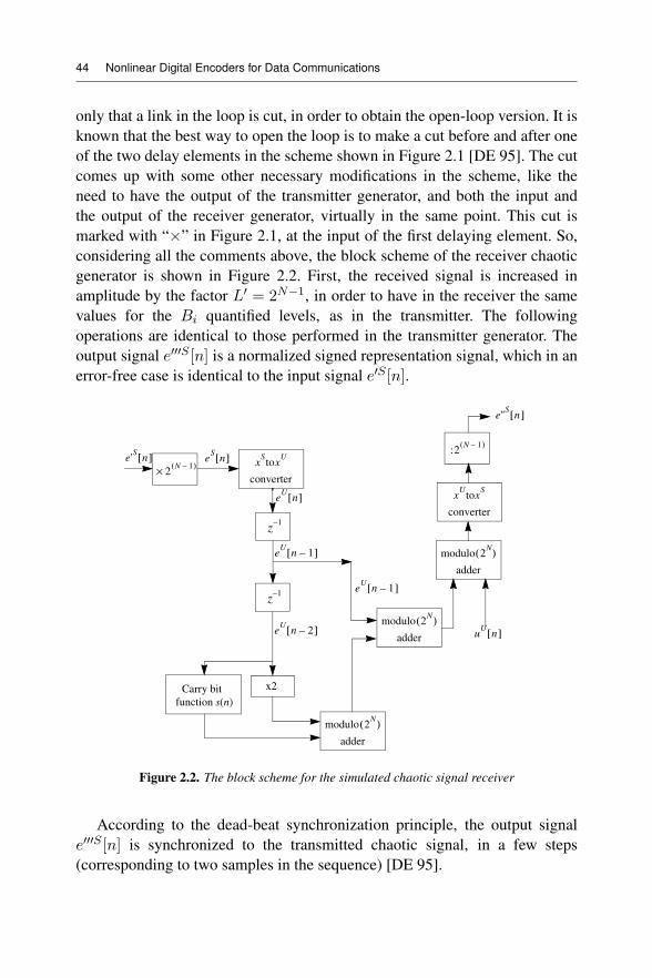
44 Nonlinear Digital Encoders for Data Communications
only that a link in the loop is cut, in order to obtain the open-loop version. It isknown that the best way to open the loop is to make a cut before and after oneof the two delay elements in the scheme shown in Figure 2.1 [DE 95]. The cutcomes up with some other necessary modifications in the scheme, like theneed to have the output of the transmitter generator, and both the input andthe output of the receiver generator, virtually in the same point. This cut ismarked with “×” in Figure 2.1, at the input of the first delaying element. So,considering all the comments above, the block scheme of the receiver chaoticgenerator is shown in Figure 2.2. First, the received signal is increased inamplitude by the factor L = 2N−1, in order to have in the receiver the samevalues for the Bi quantified levels, as in the transmitter. The followingoperations are identical to those performed in the transmitter generator. Theoutput signal e S [n] is a normalized signed representation signal, which in anerror-free case is identical to the input signal e S [n].
z1–
z1–
e'S
n[ ]
uU
n[ ]
eU
n 1–[ ]
x2Carry bit
function s(n)
modulo 2N
( )
adder
modulo 2N
( )
adder
modulo 2N
( )
adder
xU
toxS
converter
eU
n 2–[ ]
eU
n 1–[ ]
2N 1–( )
×
eS
n[ ]:2
N 1–( )
e''S
n[ ]
xStox
U
converter
eU
n[ ]
Figure 2.2. The block scheme for the simulated chaotic signal receiver
According to the dead-beat synchronization principle, the output signale S [n] is synchronized to the transmitted chaotic signal, in a few steps(corresponding to two samples in the sequence) [DE 95].
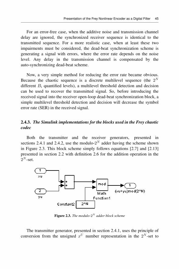
Presentation of the Frey Nonlinear Encoder as a Digital Filter 45
For an error-free case, when the additive noise and transmission channeldelay are ignored, the synchronized receiver sequence is identical to thetransmitted sequence. For a more realistic case, when at least these twoimpairments must be considered, the dead-beat synchronization scheme isgenerating a signal with errors, where the error rate depends on the noiselevel. Any delay in the transmission channel is compensated by theauto-synchronizing dead-beat scheme.
Now, a very simple method for reducing the error rate became obvious.Because the chaotic sequence is a discrete multilevel sequence (the 2N
different Bi quantified levels), a multilevel threshold detection and decisioncan be used to recover the transmitted signal. So, before introducing thereceived signal into the receiver open-loop dead-beat synchronization block, asimple multilevel threshold detection and decision will decrease the symbolerror rate (SER) in the received signal.
2.4.3. The Simulink implementations for the blocks used in the Frey chaoticcodec
Both the transmitter and the receiver generators, presented insections 2.4.1 and 2.4.2, use the modulo-2N adder having the scheme shownin Figure 2.3. This block scheme simply follows equations [2.7] and [2.13]presented in section 2.2 with definition 2.6 for the addition operation in the2N -set.
Figure 2.3. The modulo-2N adder block scheme
The transmitter generator, presented in section 2.4.1, uses the principle ofconversion from the unsigned xU number representation in the 2N -set to
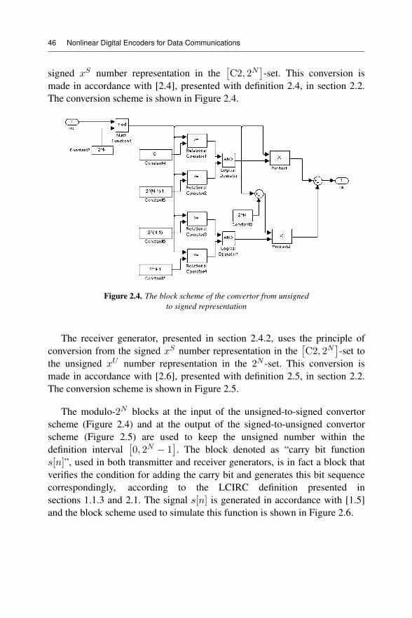
46 Nonlinear Digital Encoders for Data Communications
signed xS number representation in the C2, 2N -set. This conversion ismade in accordance with [2.4], presented with definition 2.4, in section 2.2.The conversion scheme is shown in Figure 2.4.
Figure 2.4. The block scheme of the convertor from unsignedto signed representation
The receiver generator, presented in section 2.4.2, uses the principle ofconversion from the signed xS number representation in the C2, 2N -set tothe unsigned xU number representation in the 2N -set. This conversion ismade in accordance with [2.6], presented with definition 2.5, in section 2.2.The conversion scheme is shown in Figure 2.5.
The modulo-2N blocks at the input of the unsigned-to-signed convertorscheme (Figure 2.4) and at the output of the signed-to-unsigned convertorscheme (Figure 2.5) are used to keep the unsigned number within thedefinition interval 0, 2N − 1 . The block denoted as “carry bit functions[n]”, used in both transmitter and receiver generators, is in fact a block thatverifies the condition for adding the carry bit and generates this bit sequencecorrespondingly, according to the LCIRC definition presented insections 1.1.3 and 2.1. The signal s[n] is generated in accordance with [1.5]and the block scheme used to simulate this function is shown in Figure 2.6.
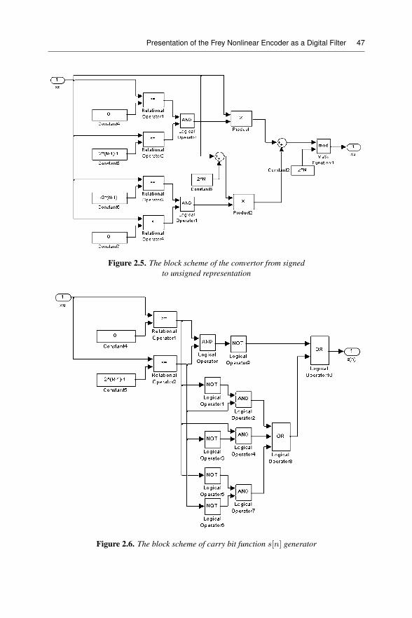
Presentation of the Frey Nonlinear Encoder as a Digital Filter 47
Figure 2.5. The block scheme of the convertor from signedto unsigned representation
Figure 2.6. The block scheme of carry bit function s[n] generator

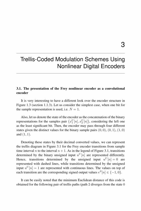
3
Trellis-Coded Modulation Schemes UsingNonlinear Digital Encoders
3.1. The presentation of the Frey nonlinear encoder as a convolutionalencoder
It is very interesting to have a different look over the encoder structure inFigure 1.3 (section 1.1.3). Let us consider the simplest case, when one bit forthe sample representation is used, i.e. N = 1.
Also, let us denote the state of the encoder as the concatenation of the binaryrepresentations for the samples pair xU1 [n], x
U2 [n] , considering the left one
as the least significant bit. Then, the encoder may pass through four differentstates given the distinct values for the binary sample pairs (0, 0), (0, 1), (1, 0)and (1, 1).
Denoting these states by their decimal converted values, we can representthe trellis diagram in Figure 3.1 for the Frey encoder transitions from sampletime interval n to the interval n+1. As in the legend of Figure 3.1, transitionsdetermined by the binary unsigned input uU [n] are represented differently.Hence, transitions determined by the unsigned input uU [n] = 0 arerepresented with dashed lines, while transitions determined by the unsignedinput uU [n] = 1 are represented with continuous lines. The values on top ofeach transition are the corresponding signed output values eS [n] ∈ {−1, 0}.
It can be easily noted that the minimum Euclidean distance of this code isobtained for the following pair of trellis paths (path 2 diverges from the state 0
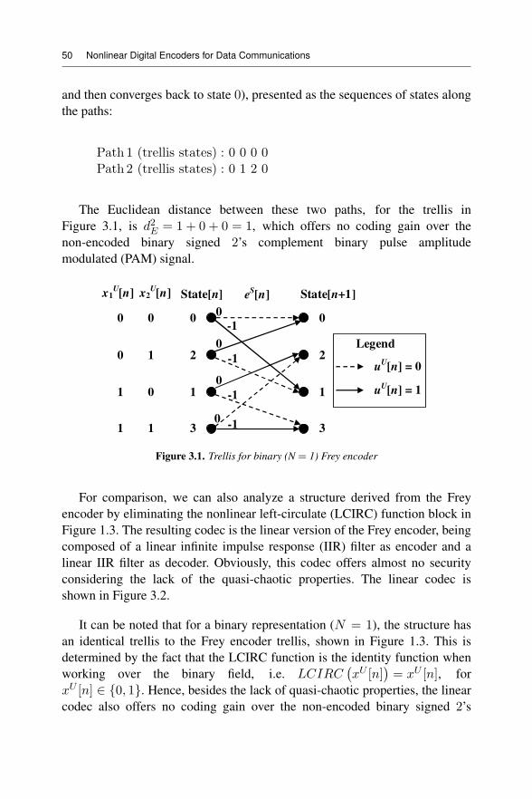
50 Nonlinear Digital Encoders for Data Communications
and then converges back to state 0), presented as the sequences of states alongthe paths:
Path 1 (trellis states) : 0 0 0 0Path 2 (trellis states) : 0 1 2 0
The Euclidean distance between these two paths, for the trellis inFigure 3.1, is d2E = 1 + 0 + 0 = 1, which offers no coding gain over thenon-encoded binary signed 2’s complement binary pulse amplitudemodulated (PAM) signal.
-1
0
0-1
-1
0
-1
00 0
State[n]
0
0 1 2
1 0 1
1 1 3
State[n+1]
0
2
1
3
x1U[n] x2
U[n] e
S[n]
Legend
uU[n] = 0
uU[n] = 1
Figure 3.1. Trellis for binary (N = 1) Frey encoder
For comparison, we can also analyze a structure derived from the Freyencoder by eliminating the nonlinear left-circulate (LCIRC) function block inFigure 1.3. The resulting codec is the linear version of the Frey encoder, beingcomposed of a linear infinite impulse response (IIR) filter as encoder and alinear IIR filter as decoder. Obviously, this codec offers almost no securityconsidering the lack of the quasi-chaotic properties. The linear codec isshown in Figure 3.2.
It can be noted that for a binary representation (N = 1), the structure hasan identical trellis to the Frey encoder trellis, shown in Figure 1.3. This isdetermined by the fact that the LCIRC function is the identity function whenworking over the binary field, i.e. LCIRC xU [n] = xU [n], forxU [n] ∈ {0, 1}. Hence, besides the lack of quasi-chaotic properties, the linearcodec also offers no coding gain over the non-encoded binary signed 2’s
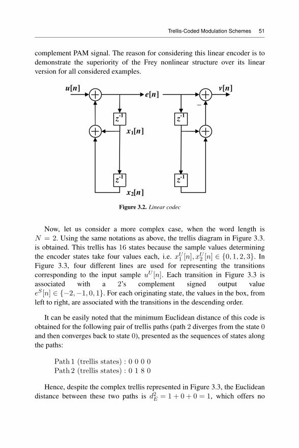
Trellis-Coded Modulation Schemes 51
complement PAM signal. The reason for considering this linear encoder is todemonstrate the superiority of the Frey nonlinear structure over its linearversion for all considered examples.
_
z-1
z-1
u[n]e[n]
x1[n]
x2[n]
z-1
z-1
v[n]
Figure 3.2. Linear codec
Now, let us consider a more complex case, when the word length isN = 2. Using the same notations as above, the trellis diagram in Figure 3.3.is obtained. This trellis has 16 states because the sample values determiningthe encoder states take four values each, i.e. xU1 [n], x
U2 [n] ∈ {0, 1, 2, 3}. In
Figure 3.3, four different lines are used for representing the transitionscorresponding to the input sample uU [n]. Each transition in Figure 3.3 isassociated with a 2’s complement signed output valueeS [n] ∈ {−2,−1, 0, 1}. For each originating state, the values in the box, fromleft to right, are associated with the transitions in the descending order.
It can be easily noted that the minimum Euclidean distance of this code isobtained for the following pair of trellis paths (path 2 diverges from the state 0and then converges back to state 0), presented as the sequences of states alongthe paths:
Path 1 (trellis states) : 0 0 0 0Path 2 (trellis states) : 0 1 8 0
Hence, despite the complex trellis represented in Figure 3.3, the Euclideandistance between these two paths is d2E = 1 + 0 + 0 = 1, which offers no
52 Nonlinear Digital Encoders for Data Communications
coding gain over the non-encoded binary signed 2’s complement PAM signal.In fact, the signed quaternary output signal eS [n] has a higher mean powerthan the binary signal. Therefore, in order to make a fair performancecomparison, the power of the transmitted signed signal eS [n] has to benormalized, for each value of N .
Let us consider the signed 2’s complement signal for any value of N .Hence, the signed signal takes equally probable valuesxS [n] ∈ {−2N−1,−2N−1 + 1, . . . ,−1, 0, 1, . . . , 2N−1 − 1}. The mean andthe variance of the signed representation signal take the following values:
xS [n] = −12
σ2xS [n]
= (xS [n])2 − xS [n]2= 22N−1+1
6 − 14 =
(22N−1)12
[3.1]
In the following, the coding performance of these trellises will be analyzedusing Ungerboeck’s rules [UNG 82], considering that all the signals arenormalized by their actual standard deviation in [3.1]. It can be noted that theminimum distance pair of paths in the Frey encoder trellis differs in onlythree transitions, and for the last two transitions, the individual distance is nullfor any value of N . Considering the above normalization, the distancebetween the two paths in the first transition takes the minimum value from thesignal set distances, i.e. 1/σ2
xS [n]= 12/ 22N − 1 . Hence, the second rule of
Ungerboeck is not fulfilled, i.e. transitions originating from the same state donot receive signals with a maximum distance. It can be noted that the outputsignal is equal (in the unsigned representation) to the least significant stateN -tuple (eU [n] = xU1 [n]). Unfortunately, the last transitions, which arejoining the same state, will receive identical signals from the same set,determining a null distance between them. This is in contradiction with thethird rule of Ungerboeck [UNG 82]. In this case, the first rule is also neverfulfilled, because the trellis is not symmetrical. Considering the fourth rule ofUngerboeck, it can be noted that there are no parallel transitions. Inconclusion, the Frey encoder does not fulfill any of Ungerboeck’s rules for anoptimum trellis design. It must be noted that the fact that the second and thethird rules are not fulfilled is not determined by the nonlinear LCIRCfunction, but because of the relation between the input and output of the Freyencoder and the first delay output x1[n]. In fact, using any other nonlinearfunction instead, or even for the linear encoder, these two rules are also notfulfilled.

Trellis-Coded Modulation Schemes 53
0 0
State[n]
0
0 1 4
0 2 8
0 3 12
Legend
uU[n] = 0
uU[n] = 1
x1U[n] x2
U[n] e
S[n]
1 0 1
1 1 5
1 2 9
1 3 13
2 0 2
2 1 6
2 2 10
2 3
3 0 3
3 1 7
3 2
3 3
14
11
15
uU[n] = 2
uU[n] = 3
4
8
12
1
5
9
13
2
6
10
3
7
14
11
15
0
State[n+1]
0/1/-2/-1
0/1/-2/-1
0/1/-2/-1
0/1/-2/-1
0/1/-2/-1
0/1/-2/-1
0/1/-2/-1
0/1/-2/-1
0/1/-2/-1
0/1/-2/-1
0/1/-2/-1
0/1/-2/-1
0/1/-2/-1
0/1/-2/-1
0/1/-2/-1
0/1/-2/-1
Figure 3.3. Trellis for quaternary (N = 2) Frey encoder
54 Nonlinear Digital Encoders for Data Communications
The binary signal trellis offers a distance of d2E,N=1,F rey = 12/3 = 4,while the quaternary signal trellis offers a distance ofd2E,N=2,F rey = 12/15 = 0.8. Therefore, quaternary signal trellis of the Freyencoder performs worse than the binary one by10log10 d2E,N=1,F rey/d
2E,N=2,F rey = 10log10 (5) ≈ 7dB.
The linear version of the Frey encoder can be analyzed for N = 2. Thetrellis for the linear encoder is shown in Figure 3.4.
Following the same normalization procedure as above, we can compute theEuclidean distance for the linear encoder with N = 2, having the trellis inFigure 3.4. The minimum Euclidean distance of this code is obtained for thefollowing pair of trellis paths presented as the sequences of states along thepaths:
Path 1 (trellis states) : 0 0 0 0Path 2 (trellis states) : 0 1 4 0
The minimum Euclidean distance for this linear encoder with N = 2 is:
d2E,N=2,linear =1√5/4
2
+ 0 + 0 = 45 = 0.8, which is equal to that of the
quaternary signal trellis of the Frey encoder. This means that both structureswork identically and worse than the binary one.
Section 3.2 presents a method for improving the Frey encoder codingperformances.
3.2. Frey encoder trellis design optimization methods for pulse amplitude– trellis-coded modulation (TCM) schemes
As it was demonstrated in section 3.1, the Frey nonlinear encoder has atrellis that does not offer any coding gain over the linear encoder and over anyusual coded system with the same complexity.
To obtain certain coding gains, we developed two distinct approaches. Forboth cases, the goal is to design the trellis following Ungerboeck’s rules ofproper set partitioning [UNG 82]. For the sake of simplicity and ease ofcomparison with the Frey’s filter, we will study only the PAM signals,represented in 2’s complement form.
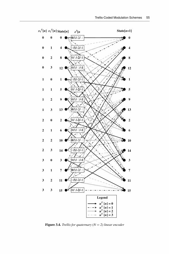
Trellis-Coded Modulation Schemes 55
0 0
State[n]
0
0 1 4
0 2 8
0 3 12
Legend
uU
[n] = 0
uU
[n] = 1
x1U[n] x2
U[n]
eS[n
1 0 1
1 1 5
1 2 9
1 3 13
2 0 2
2 1 6
2 2 10
2 3
3 0 3
3 1 7
3 2
3 3
14
11
15
uU
[n] = 2
uU
[n] = 3
4
8
12
1
5
9
13
2
6
10
3
7
14
11
15
00/1/-2/-1
0/1/-2/-1
0/1/-2/-1
0/1/-2/-1
0/1/-2/-1
0/1/-2/-1
0/1/-2/-1
0/1/-2/-1
0/1/-2/-1
0/1/-2/-1
0/1/-2/-1
0/1/-2/-1
0/1/-2/-1
0/1/-2/-1
0/1/-2/-1
0/1/-2/-1
State[n+1]
Figure 3.4. Trellis for quaternary (N = 2) linear encoder
56 Nonlinear Digital Encoders for Data Communications
In the first case, in order to fulfill the second Ungerboeck’s rule, i.e. tohave transitions originating from the same state associated with signalshaving a larger minimum distance, the input signal set is reduced, which isequivalent to an input word length decrease as compared to the output wordlength. We have to mention that in this case, the structure of the filter is notmodified, and we only need different representation code words in the inputand output. Therefore, the coding rate is decreased. This input word lengthdecrease method for proper signal set design is presented in section 3.2.1.Then, in order to increase the coding gain, a proper set partitioning for thePAM signal is needed.
To prove the coding features of these nonlinear structures, the equivalencybetween a modified GF (4) Frey encoder and an optimum conventional linearGF (2) recursive and systematic convolutional (RSC) encoder isdemonstrated in section 3.2.2. Even this equivalence is demonstrated for aparticular case; these results can be generalized. Therefore, in section 3.2.3, ageneralized block scheme for optimum PAM-TCM encoder is provided.
The second trellis optimization method is introduced in section 3.2.4. Thismethod assumes keeping the same representation word length throughout thewhole structure and modifying the encoder in order to have two outputs insteadof one. Hence, an encoder having an encoding rate of 1/2 is obtained. Also,the signal will be transmitted in the quadrature amplitude shift keying (QASK)form with 2’s complement representation for both branches. Here, the codinggain is increased also by proper signal set partitioning.
3.2.1. Increasing the coding gain by reducing the representation code wordlength in the input
Now, let us analyze in depth the encoders introduced in section 3.1. Eachof these schemes has a trellis that denotes a convolutional encoder similarity.For these schemes, which are in fact finite precision digital filters, we can evendefine an encoding rate as the ratio between the input word length Nin and theoutput word length Nout:
RNNin
Nout[3.2]
Using [3.2], it results that all the codes in section 3.1 have an encodingrate equal to 1 because the input, the internal processing and the output word
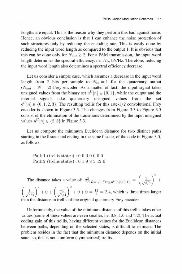
Trellis-Coded Modulation Schemes 57
lengths are equal. This is the reason why they perform this bad against noise.Hence, an obvious conclusion is that 1 can enhance the noise protection ofsuch structures only by reducing the encoding rate. This is easily done byreducing the input word length as compared to the output 1. It is obvious thatthis can be done only for Nout ≥ 2. For a PAM transmission, the input wordlength determines the spectral efficiency, i.e. Nin b/s/Hz. Therefore, reducingthe input word length also determines a spectral efficiency decrease.
Let us consider a simple case, which assumes a decrease in the input wordlength from 2 bits per sample to Nin = 1 for the quaternary output(Nout = N = 2) Frey encoder. As a matter of fact, the input signal takesunsigned values from the binary set uU [n] ∈ {0, 1}, while the output and theinternal signals take quaternary unsigned values from the seteU [n] ∈ {0, 1, 2, 3}. The resulting trellis for this rate-1/2 convolutional Freyencoder is shown in Figure 3.5. The changes from Figure 3.3 to Figure 3.5consist of the elimination of the transitions determined by the input unsignedvalues uU [n] ∈ {2, 3} in Figure 3.3.
Let us compute the minimum Euclidean distance for two distinct pathsstarting in the 0 state and ending in the same 0 state, of the code in Figure 3.5,as follows:
Path 1 (trellis states) : 0 0 0 0 0 0 0Path 2 (trellis states) : 0 1 9 8 3 12 0
The distance takes a value of: d2E,R=1/2,F rey,uU [n]∈{0,1} = 1√
5/4
2
+
1√5/4
2
+ 0 + −1√5/4
2
+ 0 + 0 = 125 = 2.4, which is three times larger
than the distance in trellis of the original quaternary Frey encoder.
Unfortunately, the value of the minimum distance of this trellis takes othervalues (some of these values are even smaller, i.e. 0.8, 1.6 and 7.2). The actualcoding gain of this trellis, having different values for the Euclidean distancesbetween paths, depending on the selected states, is difficult to estimate. Theproblem resides in the fact that the minimum distance depends on the initialstate; so, this is not a uniform (symmetrical) trellis.
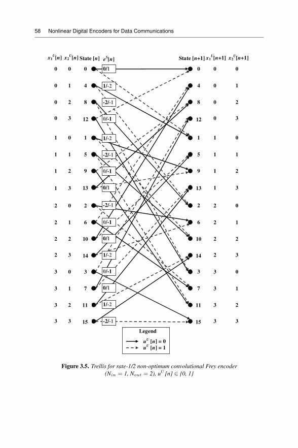
58 Nonlinear Digital Encoders for Data Communications
0 0
State [n]
0
0 1 4
0 2 8
0 3 12
Legend
uU
[n] = 0
uU
[n] = 1
x1U[n] x2
U[n] e
S[n]
1 0 1
1 1 5
1 2 9
1 3 13
2 0 2
2 1 6
2 2 10
2 3
3 0 3
3 1 7
3 2
3 3
14
11
15
0 1
0 2
0 3
1 0
1 1
1 2
1 3
2 0
2 1
2 2
2 3
3 0
3 1
3 2
3 3
4
8
12
1
5
9
13
2
6
10
3
7
14
11
15
0 0 0
State [n+1] x1U[n+1] x2
U[n+1]
1/-2
-2/-1
0/-1
1/-2
-2/-1
0/-1
0/1
-2/-1
0/-1
0/1
1/-2
0/-1
0/1
1/-2
-2/-1
0/1
Figure 3.5. Trellis for rate-1/2 non-optimum convolutional Frey encoder(Nin = 1, Nout = 2), uU [n] ∈ {0, 1}
Trellis-Coded Modulation Schemes 59
However, this gain over the original quaternary Frey encoder is determinedby the scarcity increase in the trellis structure, determined by the elimination ofhalf the number of possible transitions. Therefore, this increases the minimumdistance between different paths. As it is shown later, this is not the largest gainthat can be achieved by the encoding rate reducing in these schemes, becausethe set partitioning optimization rules were not considered.
In the following, the best performance case is determined for a rate-1/2Frey encoder, with the input word length of Nin = 1 and quaternary output(Nout = N = 2). For the best Frey encoder with these parameters, the inputsignal takes unsigned values from the binary set uU [n] ∈ {0, 2}, while theoutput and the internal signals take quaternary unsigned values from the seteU [n] ∈ {0, 1, 2, 3}. The resulting trellis for the best rate-1/2 Frey encoderis obtained by eliminating the transitions determined by the input unsignedvalues uU [n] ∈ {1, 3} from Figure 3.3. The resulting trellis for this best rate-1/2 convolutional Frey encoder is shown in Figure 3.6.
For the sake of clarity, let us consider the following pair of two paths, bothstarting in state 3 and ending in state 6:
Path 1 (trellis states) : 3 13 8 0 0 2 6Path 2 (trellis states) : 3 15 12 3 13 10 6
The Euclidean distance between the above pair of paths of the code isdetermined as
d2E,R=1/2,F rey,uU [n]∈{0,2} =2
5/4
2
+ 0 +1
5/4
2
+−1
5/4
2
+ 0 + 0 = 6/ 5/42= 4.8.
In fact, this is the minimum value of the Euclidean distance for the code inFigure 3.6.
We noted that starting from any state, there is a unique pair of paths in thetrellis ending in any state (from all 16) after six transitions, having the sameminimum distance. Hence, we can say that this is a uniform (symmetrical)trellis. In fact, this gain is explained by the proper set partitioning of the
60 Nonlinear Digital Encoders for Data Communications
output signal set. The selected transitions in the trellis (uU [n] ∈ {0, 2}) willdetermine the output signal pairs, for the transitions starting from the samestate, to have the maximum distance between them. In the 2’s complementrepresentation, the output pairs of maximum distance are (1,−1) and (0,−2).The Euclidean distance increases at least by a factor of 4 as compared to thedistance of the original quaternary Frey encoder. Hence, the second rule ofUngerboeck is fulfilled, i.e. transitions originating from the same state havesignals assigned from sets with a maximum distance between the elements. Inaddition, we can note that the output signal is equal (in the unsignedrepresentation) to the least significant state tuple (eU [n] = xU1 [n]). Forexample, all transitions having the eS [n] = −2 output signal assigned willconverge in a state having xU1 [n] = 2. Unfortunately, the transitions joiningthe same state will receive identical signals from the same set. This is incontradiction with the third rule of Ungerboeck. We can note that theseencoders do not fulfill this rule by de facto. To end the analysis of thisstructure following the rules of Ungerboeck, we have to mention that the firstrule is never fulfilled in the reduced input code word approach, because thetrellis is no longer symmetrical (see Figure 3.6). This fact also reduces thecoding gain of the structure. Considering the fourth rule of Ungerboeck, wemust note that we cannot have parallel transitions in this structure because theencoder is not systematic (we do not have unfiltered samples) at the output.
The best rate-1/2 (Nin = 1, Nout = 2) Frey encoder performs better thanthe quaternary Frey encoder, having a coding gain of
10log10 d2E,R=1/2,F rey,uU [n]∈{0,2}/d2E,N=2,Frey
= 10log10 (6) ≈ 7.78dB,
which outperforms the signed binary output signal trellis by10log10 (4.8/4) ≈ 0.79dB.
As in section 3.1, let us consider the linear rate-1/2 convolutional linearencoder (Nin = 1, Nout = 2), following the same set partitioningoptimization procedure as for the similar Frey encoder, i.e. the set of selectedinputs is uU [n] ∈ {0, 2}. In this case, the trellis is less efficient than that ofthe Frey encoder, having a smaller minimum Euclidean distance. Theresulting trellis for the rate-1/2 linear encoder with input unsigned samplesvalues uU [n] ∈ {0, 2} is shown in Figure 3.7.
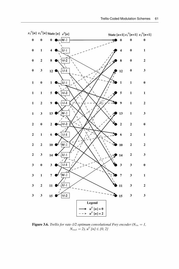
Trellis-Coded Modulation Schemes 61
0 0
State [n]
0
0 1 4
0 2 8
0 3 12
Legend
uU
[n] = 0
x1U[n] x2
U[n]
eS[n]
1 0 1
1 1 5
1 2 9
1 3 13
2 0 2
2 1 6
2 2 10
2 3
3 0 3
3 1 7
3 2
3 3
14
11
15
uU
[n] = 2
0 1
0 2
0 3
1 0
1 1
1 2
1 3
2 0
2 1
2 2
2 3
3 0
3 1
3 2
3 3
4
8
12
1
5
9
13
2
6
10
3
7
14
11
15
0 0 0
1/-1
0/-2
1/-1
1/-1
0/-2
1/-1
0/-2
0/-2
1/-1
0/-2
1/-1
1/-1
0/-2
1/-1
0/-2
0/-2
State [n+1] x1U[n+1] x2
U[n+1]
Figure 3.6. Trellis for rate-1/2 optimum convolutional Frey encoder (Nin = 1,Nout = 2), uU [n] ∈ {0, 2}
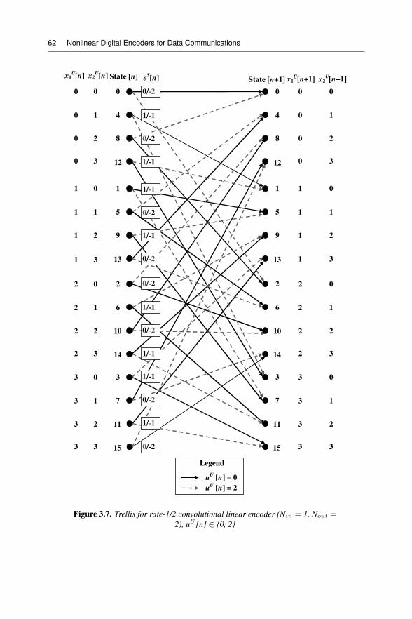
62 Nonlinear Digital Encoders for Data Communications
0 0
State [n]
0
0 1 4
0 2 8
0 3 12
Legend
uU
[n] = 0
x1U[n] x2
U[n] e
S[n]
1 0 1
1 1 5
1 2 9
1 3 13
2 0 2
2 1 6
2 2 10
2 3
3 0 3
3 1 7
3 2
3 3
14
11
15
uU
[n] = 2
0 1
0 2
0 3
1 0
1 1
1 2
1 3
2 0
2 1
2 2
2 3
3 0
3 1
3 2
3 3
4
8
12
1
5
9
13
2
6
10
3
7
14
11
15
0 0 0
1/-1
0/-2
1/-1
1/-1
0/-2
1/-1
0/-2
0/-2
1/-1
0/-2
1/-1
1/-1
0/-2
1/-1
0/-2
0/-2
State [n+1] x1U[n+1] x2
U[n+1]
Figure 3.7. Trellis for rate-1/2 convolutional linear encoder (Nin = 1, Nout =2), uU [n] ∈ {0, 2}
Trellis-Coded Modulation Schemes 63
Comparing the trellises in Figures 3.6 and 3.7, we can easily see that theabsence of the LCIRC block affects transitions (changes the next state)originating from states having xU1 [n] ∈ {1, 2} (initial states placed in themiddle) and it does not change the output values eS [n] associated with aspecific initial state. This is explained by the fact that the LCIRC functionchanges only the value of xU2 [n+ 1] without changing the other variables (seethe linear encoder scheme in Figure 3.2).
For example, let us consider the following pair of two paths for the trellisin Figure 3.7, having the minimum Euclidean distance, both starting in state 3and ending in state 1:
Path 1 (trellis states) : 3 15 12 1Path 2 (trellis states) : 3 13 4 1
The Euclidean distance between these paths is:
d2E,R=1/2,linear,uU [n]∈{0,2} = −2√
5/4
2
+ 2√5/4
2
+ 0 = 4/ 5/42=
3.2, which is four times larger than the distance in the trellis of the originalquaternary linear encoder. The same result is obtained for the input setuU [n] ∈ {1, 3}. However, the rate-1/2 convolutional linear encoder inFigure 3.7 performs worse than the corresponding rate-1/2 convolutionalFrey encoder, having an encoding loss of10log10 d2
E,R=1/2,F rey,uU [n]∈{0,2} / d2E,R=1/2,linear,uU [n]∈{0,2} =
10log10 (6/4) ≈ 1.76 dB. When compared to the signed binary output signaltrellis, we also have a loss of 10log10 (4/3.2) ≈ 0.97 dB. Using the inversesystem proposed by Frey for the sample decoding [FRE 93], the sameperformance is noted as for the rate 1, N = 2 encoder.
We also studied the larger word length encoders, but the results were notsatisfactory. The complexity increase in the trellis (the number of states) isnot really exploited in the Frey encoder case. Actually, we can generalize theFrey encoder trellis’ parameters for the scheme in Figure 1.3 (section 1.1.3)for any pair of values for the input and output representation code words, i.e.1 < Nin ≤ Nout = N .
Now, let us consider a rate-1/2 convolutional Frey encoder, having Nin = 2bits per sample in the input and a 16 levels output signal (Nout = 4). Using
64 Nonlinear Digital Encoders for Data Communications
the above-mentioned set partitioning method, we select the quaternary set forthe input signal, i.e., uU [n] ∈ {0, 4, 8, 12}, while the output and the internalsignals take 16 unsigned values from the set eU [n] ∈ {0, 1, 2, . . . , 15}. Theresulting trellis for the rate-1/2 convolutional Frey encoder has 256 states, andits graphical analysis is too difficult. However, we can compute the minimumEuclidean distance of the trellis as for the previous cases. Let us consider thefollowing pair of paths, both starting in state 1 and ending in state 105:
Path 1 (trellis states) : 1 33 35 105Path 2 (trellis states) : 1 37 163 105
This trellis offers a minimum distance, also determined between the aboveconsidered two paths, with the value: d2
E,R=1/2,F rey,uU [n]∈{0,4,8,12} =
−4√85/4
2
+ 0 + 0 = 16/ 85/42 ≈ 0.753. The same result is obtained,
for example, when the input set is either uU [n] ∈ {1, 5, 9, 13},uU [n] ∈ {2, 6, 10, 14} or uU [n] ∈ {3, 7, 11, 15}.
We can note that rate-1/2 convolutional Frey encoder (Nin = 2,Nout = 4) is performing worse than the rate-1/2 convolutional Frey encoder(Nin = 1, Nout = 2), the last one having an encoding gain of10log10 d2
E,R=1/2,F rey,uU [n]∈{0,2}/d2E,R=1/2,F rey,uU [n]∈{0,4,8,12} =
10log104.8
64/85 ≈ 8.05 dB .
The conclusion here is that, even if a good signal set partitioning was used,for larger sizes of representation word length, the output signal set increasesexponentially with 2Nout, which reduces the minimum distance of the 2Nout-PAM signal symbols accordingly. The Frey encoder trellis cannot overcomethis reduction in the protection against noise. As noted in the previous example,even if the distance between the paths is 16 times larger than the distance inthe non-encoded signal, the exponential decrease in the later symbol distancealso reduces the whole trellis minimum Euclidean distance. Also, this happensdue to the lack of symmetry in the trellis and null distance over the transitionsconverging into the same state.
We can conclude here that the Frey encoder cannot offer betterperformances for higher word lengths in the output, and therefore the binaryand optimum quaternary cases remain the best encoders.
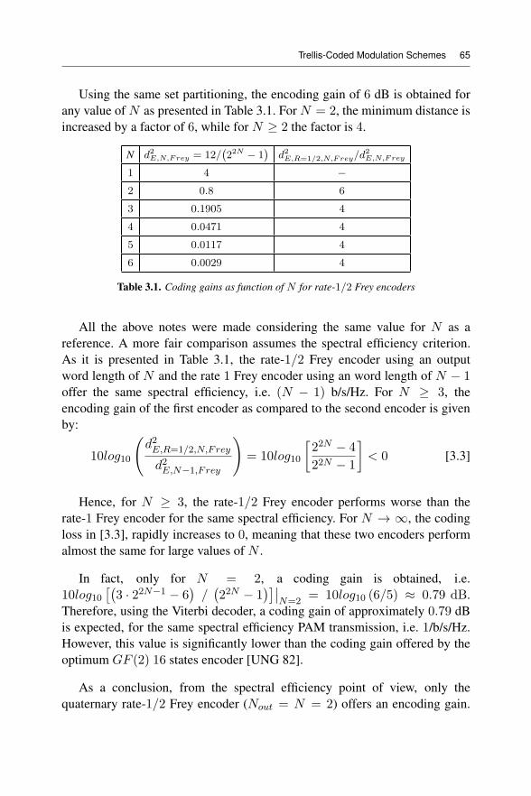
Trellis-Coded Modulation Schemes 65
Using the same set partitioning, the encoding gain of 6 dB is obtained forany value of N as presented in Table 3.1. For N = 2, the minimum distance isincreased by a factor of 6, while for N ≥ 2 the factor is 4.
N d2E,N,Frey = 12/ 22N − 1 d2E,R=1/2,N,Frey/d2E,N,Frey
1 4 −2 0.8 6
3 0.1905 4
4 0.0471 4
5 0.0117 4
6 0.0029 4
Table 3.1. Coding gains as function of N for rate-1/2 Frey encoders
All the above notes were made considering the same value for N as areference. A more fair comparison assumes the spectral efficiency criterion.As it is presented in Table 3.1, the rate-1/2 Frey encoder using an outputword length of N and the rate 1 Frey encoder using an word length of N − 1offer the same spectral efficiency, i.e. (N − 1) b/s/Hz. For N ≥ 3, theencoding gain of the first encoder as compared to the second encoder is givenby:
10log10d2E,R=1/2,N,Frey
d2E,N−1,F rey
= 10log1022N − 4
22N − 1< 0 [3.3]
Hence, for N ≥ 3, the rate-1/2 Frey encoder performs worse than therate-1 Frey encoder for the same spectral efficiency. For N → ∞, the codingloss in [3.3], rapidly increases to 0, meaning that these two encoders performalmost the same for large values of N .
In fact, only for N = 2, a coding gain is obtained, i.e.10log10 3 · 22N−1 − 6 / 22N − 1
N=2= 10log10 (6/5) ≈ 0.79 dB.
Therefore, using the Viterbi decoder, a coding gain of approximately 0.79 dBis expected, for the same spectral efficiency PAM transmission, i.e. 1/b/s/Hz.However, this value is significantly lower than the coding gain offered by theoptimum GF (2) 16 states encoder [UNG 82].
As a conclusion, from the spectral efficiency point of view, only thequaternary rate-1/2 Frey encoder (Nout = N = 2) offers an encoding gain.
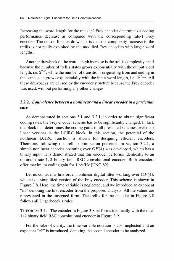
66 Nonlinear Digital Encoders for Data Communications
Increasing the word length for the rate-1/2 Frey encoder determines a codingperformance decrease as compared with the corresponding rate-1 Freyencoder. The reason for this drawback is that the complexity increase in thetrellis is not really exploited by the modified Frey encoders with larger wordlengths.
Another drawback of the word length increase is the trellis complexity itselfbecause the number of trellis states grows exponentially with the output wordlength, i.e. 22N , while the number of transitions originating from and ending inthe same state grows exponentially with the input word length, i.e. 22Nin . Allthese drawbacks are caused by the encoder structure because the Frey encoderwas used, without performing any other changes.
3.2.2. Equivalence between a nonlinear and a linear encoder in a particularcase
As demonstrated in sections 3.1 and 3.2.1, in order to obtain significantcoding rates, the Frey encoder scheme has to be significantly changed. In fact,the block that determines the coding gains of all presented schemes over theirlinear versions is the LCIRC block. In this section, the potential of thenonlinear LCIRC function is shown for designing efficient encoders.Therefore, following the trellis optimization presented in section 3.2.1, asimple nonlinear encoder operating over GF (4) was developed, which has abinary input. It is demonstrated that this encoder performs identically to anoptimum rate-1/2 binary field RSC convolutional encoder. Both encodersoffer maximum coding gain for 1 b/s/Hz [UNG 82].
Let us consider a first-order nonlinear digital filter working over GF (4),which is a simplified version of the Frey encoder. This scheme is shown inFigure 3.8. Here, the time variable is neglected, and we introduce an exponent“c1” denoting the first encoder from the proposed analysis. All the values arerepresented in the unsigned form. The trellis for the encoder in Figure 3.8follows all Ungerboeck’s rules.
THEOREM 3.1.– The encoder in Figure 3.8 performs identically with the rate-1/2 binary field RSC convolutional encoder in Figure 3.9.
For the sake of clarity, the time variable notation is also neglected and anexponent “c2” is introduced, denoting the second encoder to be analyzed.
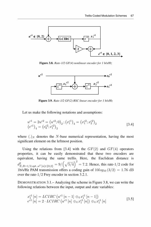
Trellis-Coded Modulation Schemes 67
uc1
∈∈∈∈ {0, 2}z
-1LCIRC
ec1
∈∈∈∈ {0, 1, 2, 3}
x1c1
2
Figure 3.8. Rate-1/2 GF(4) nonlinear encoder for 1 b/s/Hz
x1c2
z-1
uc2
e0c2
x2c2
z-1
e1c2
Figure 3.9. Rate-1/2 GF(2) RSC linear encoder for 1 b/s/Hz
Let us make the following notations and assumptions:
uc1 = 2uc2 = uc2; 02; xc11 4
= xc21 ;xc22 2ec1
4= ec20 ; ec21 2
[3.4]
where (.)N denotes the N -base numerical representation, having the mostsignificant element on the leftmost position.
Using the relations from [3.4] with the GF (2) and GF (4) operatorsproperties, it can be easily demonstrated that these two encoders areequivalent, having the same trellis. Here, the Euclidean distance is
d2E,R=1/2,opt.,uU [n]∈{0,2} = 9/ 5/4
2= 7.2. Hence, this rate-1/2 code for
1b/s/Hz PAM transmission offers a coding gain of 10log10 (3/2) = 1.76 dBover the rate-1/2 Frey encoder in section 3.2.1.
DEMONSTRATION 3.1.– Analyzing the scheme in Figure 3.8, we can write thefollowing relations between the input, output and state variables:
xc11 [n] = LCIRC uc1 [n− 1] ⊕4 xc11 [n− 1]
ec1 [n] = 2 · LCIRC uc1 [n] ⊕4 xc11 [n] ⊕4 x
c11 [n]
[3.5]
68 Nonlinear Digital Encoders for Data Communications
where “ · ” denotes the simple product (algebraic), the LCIRC function isexpressed as in definition 1.2 (section 1.1.3) with the properties presented insection 2.3, and the “⊕M” operator is the modulo-M adder given bydefinition 2.6 (section 2.2).
From the scheme in Figure 3.9, we have the following relations betweenthe input, output and state variables:
xc21 [n] = xc22 [n− 1]xc22 [n] = xc21 [n− 1] ⊕2 u
c2 [n− 1]ec20 [n] = uc2 [n]ec21 [n] = xc22 [n]
[3.6]
Introducing [3.4] and [3.6] in [3.5], the latter can be rewritten as:
xc21 ; xc22 2[n] =
LCIRC{ uc2 [n− 1] ⊕2 xc21 [n− 1] ⊕2 0 · xc22 [n− 1] ;
0⊕2 xc22 [n− 1]
2} =
xc22 [n− 1]; uc2 [n− 1]⊕2 xc21 [n− 1]
2⇒
xc21 [n] = xc22 [n− 1]xc22 [n] = uc2 [n− 1] ⊕2 x
c21 [n− 1]
ec20 ; ec21 2[n] =
2 · LCIRC{ uc2 [n] ⊕2 xc21 [n] ⊕2 0 · xc22 [n] ;
0⊕2 xc22 [n]
2}⊕4 xc21 ; xc22 2
[n] =
xc22 [n] ; uc2 [n] ⊕2 xc21 [n]
2⊕4 xc22 [n] ;
uc2 [n] ⊕2 xc21 [n]
2⊕4 xc21 ; xc22 2
[n] =
xc22 [n] ⊕2 xc22 [n] ⊕2 uc2 [n] ⊕2 x
c21 [n] ·
uc2 [n] ⊕2 xc21 [n] ;
uc2 [n] ⊕2 xc21 [n] ⊕2 u
c2 [n] ⊕2 xc21 [n]
2⊕4
⊕4 xc21 ; xc22 2[n] =
uc2 [n] ⊕2 xc21 [n] · uc2 [n] ⊕2 x
c21 [n] ⊕2 x
c21 [n] ⊕2
0 · xc22 [n] ; 0⊕2 xc22 [n− 1]
2⇒
ec20 [n] = uc2 [n]ec21 [n] = xc22 [n]
[3.7]
In [3.7], the relations given in [3.8] between the “⊕4”, “⊕2” and “·”operators were used. If a⊕4 b = c, where a, b, c ∈ {0, 1, 2, 3} and denoting
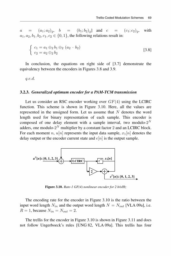
Trellis-Coded Modulation Schemes 69
a = (a1; a2)2, b = (b1; b2)2] and c = (c1; c2)2, witha1, a2, b1, b2, c1, c2 ∈ {0, 1}, the following relations result in:
c1 = a1⊕2 b1⊕2 (a2 · b2)c2 = a2⊕2 b2
[3.8]
In conclusion, the equations on right side of [3.7] demonstrate theequivalency between the encoders in Figures 3.8 and 3.9.
q.e.d.
3.2.3. Generalized optimum encoder for a PAM-TCM transmission
Let us consider an RSC encoder working over GF (4) using the LCIRCfunction. This scheme is shown in Figure 3.10. Here, all the values arerepresented in the unsigned form. Let us assume that N denotes the wordlength used for binary representation of each sample. This encoder iscomposed of one delay element with a sample interval, two modulo-2N
adders, one modulo-2N multiplier by a constant factor 2 and an LCIRC block.For each moment n, u[n] represents the input data sample, x1[n] denotes thedelay output or the encoder current state and e[n] is the output sample.
uU[n]∈{0, 1, 2, 3}
z-1
LCIRC
eU[n]∈{0, 1, 2, 3}
x1[n]
2
Figure 3.10. Rate-1 GF(4) nonlinear encoder for 2 b/s/Hz
The encoding rate for the encoder in Figure 3.10 is the ratio between theinput word length Nin and the output word length N = Nout [VLA 09a], i.e.R = 1, because Nin = Nout = 2.
The trellis for the encoder in Figure 3.10 is shown in Figure 3.11 and doesnot follow Ungerboeck’s rules [UNG 82, VLA 09a]. This trellis has four
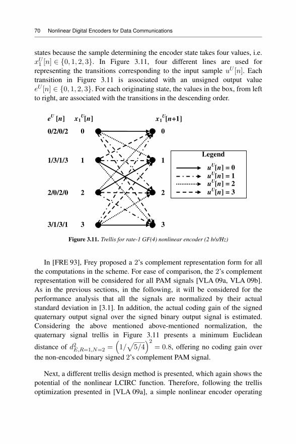
70 Nonlinear Digital Encoders for Data Communications
states because the sample determining the encoder state takes four values, i.e.xU1 [n] ∈ {0, 1, 2, 3}. In Figure 3.11, four different lines are used forrepresenting the transitions corresponding to the input sample uU [n]. Eachtransition in Figure 3.11 is associated with an unsigned output valueeU [n] ∈ {0, 1, 2, 3}. For each originating state, the values in the box, from leftto right, are associated with the transitions in the descending order.
0/2/0/2 0
1
2
3
0
1
2
3
eU
[n] x1U[n] x1
U[n+1]
Legend
uU[n] = 0
uU[n] = 1
uU[n] = 2
uU[n] = 3
1/3/1/3
2/0/2/0
3/1/3/1
Figure 3.11. Trellis for rate-1 GF(4) nonlinear encoder (2 b/s/Hz)
In [FRE 93], Frey proposed a 2’s complement representation form for allthe computations in the scheme. For ease of comparison, the 2’s complementrepresentation will be considered for all PAM signals [VLA 09a, VLA 09b].As in the previous sections, in the following, it will be considered for theperformance analysis that all the signals are normalized by their actualstandard deviation in [3.1]. In addition, the actual coding gain of the signedquaternary output signal over the signed binary output signal is estimated.Considering the above mentioned above-mentioned normalization, thequaternary signal trellis in Figure 3.11 presents a minimum Euclidean
distance of d2E,R=1,N=2 = 1/ 5/42= 0.8, offering no coding gain over
the non-encoded binary signed 2’s complement PAM signal.
Next, a different trellis design method is presented, which again shows thepotential of the nonlinear LCIRC function. Therefore, following the trellisoptimization presented in [VLA 09a], a simple nonlinear encoder operating
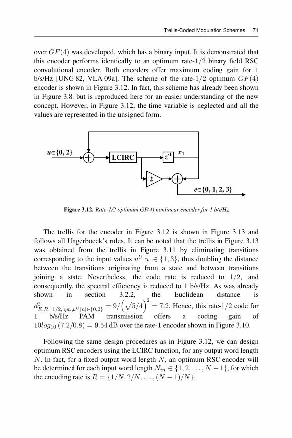
Trellis-Coded Modulation Schemes 71
over GF (4) was developed, which has a binary input. It is demonstrated thatthis encoder performs identically to an optimum rate-1/2 binary field RSCconvolutional encoder. Both encoders offer maximum coding gain for 1b/s/Hz [UNG 82, VLA 09a]. The scheme of the rate-1/2 optimum GF (4)encoder is shown in Figure 3.12. In fact, this scheme has already been shownin Figure 3.8, but is reproduced here for an easier understanding of the newconcept. However, in Figure 3.12, the time variable is neglected and all thevalues are represented in the unsigned form.
u∈{0, 2}z
-1LCIRC
e∈{0, 1, 2, 3}
x1
2
Figure 3.12. Rate-1/2 optimum GF(4) nonlinear encoder for 1 b/s/Hz
The trellis for the encoder in Figure 3.12 is shown in Figure 3.13 andfollows all Ungerboeck’s rules. It can be noted that the trellis in Figure 3.13was obtained from the trellis in Figure 3.11 by eliminating transitionscorresponding to the input values uU [n] ∈ {1, 3}, thus doubling the distancebetween the transitions originating from a state and between transitionsjoining a state. Nevertheless, the code rate is reduced to 1/2, andconsequently, the spectral efficiency is reduced to 1 b/s/Hz. As was alreadyshown in section 3.2.2, the Euclidean distance is
d2E,R=1/2,opt.,uU [n]∈{0,2} = 9/ 5/4
2= 7.2. Hence, this rate-1/2 code for
1 b/s/Hz PAM transmission offers a coding gain of10log10 (7.2/0.8) = 9.54 dB over the rate-1 encoder shown in Figure 3.10.
Following the same design procedures as in Figure 3.12, we can designoptimum RSC encoders using the LCIRC function, for any output word lengthN . In fact, for a fixed output word length N , an optimum RSC encoder willbe determined for each input word length Nin ∈ {1, 2, . . . , N − 1}, for whichthe encoding rate is R = {1/N, 2/N, . . . , (N − 1)/N}.
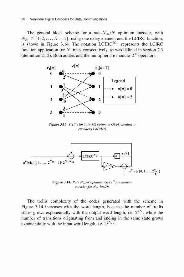
72 Nonlinear Digital Encoders for Data Communications
The general block scheme for a rate-Nin/N optimum encoder, withNin ∈ {1, 2, . . . , N − 1}, using one delay element and the LCIRC function,is shown in Figure 3.14. The notation LCIRCNin represents the LCIRCfunction application for N times consecutively, as was defined in section 2.3(definition 2.12). Both adders and the multiplier are modulo-2N operators.
3
1
32
2
1
0
00
1
2
3
0
1
2
3
e[n]
Legend
u[n] = 0
u[n] = 2
x1[n] x1[n+1]
Figure 3.13. Trellis for rate-1/2 optimum GF(4) nonlinearencoder (1 b/s/Hz)
uU[n]∈{0, 1, …, 12 −inN
}· inNN −2
inNN −2
z-1
eU[n]∈{0, 1, …, 2
N–1}
x1[n]inN
LCIRC
Figure 3.14. Rate Nin/N optimum GF(2N ) nonlinearencoder for Nin b/s/Hz
The trellis complexity of the codes generated with the scheme inFigure 3.14 increases with the word length, because the number of trellisstates grows exponentially with the output word length, i.e. 22N , while thenumber of transitions originating from and ending in the same state growsexponentially with the input word length, i.e. 22Nin .
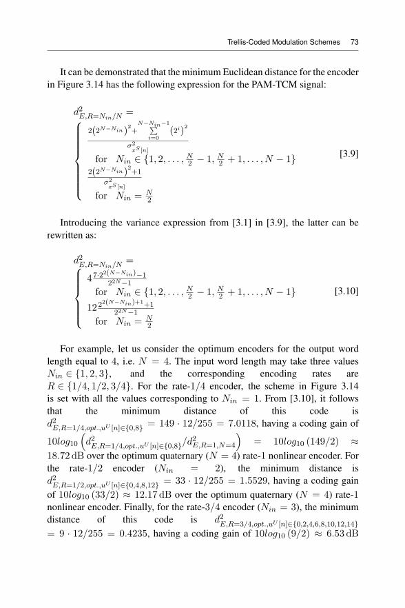
Trellis-Coded Modulation Schemes 73
It can be demonstrated that the minimum Euclidean distance for the encoderin Figure 3.14 has the following expression for the PAM-TCM signal:
d2E,R=Nin/N=⎧⎪⎪⎪⎪⎪⎪⎪⎨⎪⎪⎪⎪⎪⎪⎪⎩
2(2N−Nin)2+
N−Nin−1
i=0(2i)
2
σ2xS [n]
for Nin ∈ {1, 2, . . . , N2 − 1, N2 + 1, . . . , N − 1}2(2N−Nin)
2+1
σ2xS [n]
for Nin = N2
[3.9]
Introducing the variance expression from [3.1] in [3.9], the latter can berewritten as:
d2E,R=Nin/N=⎧⎪⎪⎪⎪⎨⎪⎪⎪⎪⎩
47·22(N−Nin)−122N−1
for Nin ∈ {1, 2, . . . , N2 − 1, N2 + 1, . . . , N − 1}1222(N−Nin)+1+1
22N−1
for Nin = N2
[3.10]
For example, let us consider the optimum encoders for the output wordlength equal to 4, i.e. N = 4. The input word length may take three valuesNin ∈ {1, 2, 3}, and the corresponding encoding rates areR ∈ {1/4, 1/2, 3/4}. For the rate-1/4 encoder, the scheme in Figure 3.14is set with all the values corresponding to Nin = 1. From [3.10], it followsthat the minimum distance of this code isd2E,R=1/4,opt.,uU [n]∈{0,8} = 149 · 12/255 = 7.0118, having a coding gain of
10log10 d2E,R=1/4,opt.,uU [n]∈{0,8}/d
2E,R=1,N=4 = 10log10 (149/2) ≈
18.72 dB over the optimum quaternary (N = 4) rate-1 nonlinear encoder. Forthe rate-1/2 encoder (Nin = 2), the minimum distance isd2E,R=1/2,opt.,uU [n]∈{0,4,8,12} = 33 · 12/255 = 1.5529, having a coding gain
of 10log10 (33/2) ≈ 12.17 dB over the optimum quaternary (N = 4) rate-1nonlinear encoder. Finally, for the rate-3/4 encoder (Nin = 3), the minimumdistance of this code is d2
E,R=3/4,opt.,uU [n]∈{0,2,4,6,8,10,12,14}= 9 · 12/255 = 0.4235, having a coding gain of 10log10 (9/2) ≈ 6.53 dB
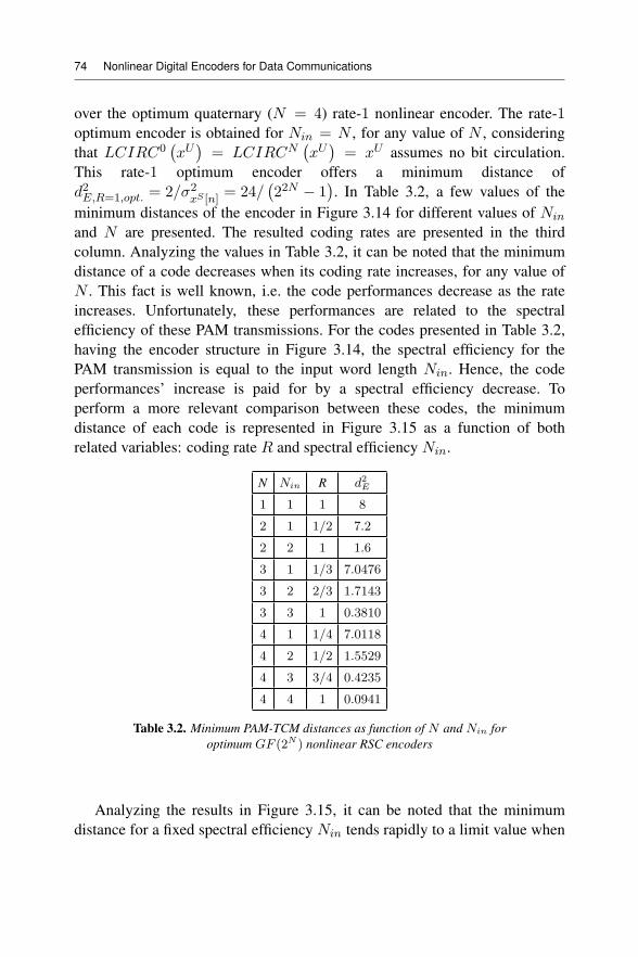
74 Nonlinear Digital Encoders for Data Communications
over the optimum quaternary (N = 4) rate-1 nonlinear encoder. The rate-1optimum encoder is obtained for Nin = N , for any value of N , consideringthat LCIRC0 xU = LCIRCN xU = xU assumes no bit circulation.This rate-1 optimum encoder offers a minimum distance ofd2E,R=1,opt. = 2/σ2
xS [n]= 24/ 22N − 1 . In Table 3.2, a few values of the
minimum distances of the encoder in Figure 3.14 for different values of Nin
and N are presented. The resulted coding rates are presented in the thirdcolumn. Analyzing the values in Table 3.2, it can be noted that the minimumdistance of a code decreases when its coding rate increases, for any value ofN . This fact is well known, i.e. the code performances decrease as the rateincreases. Unfortunately, these performances are related to the spectralefficiency of these PAM transmissions. For the codes presented in Table 3.2,having the encoder structure in Figure 3.14, the spectral efficiency for thePAM transmission is equal to the input word length Nin. Hence, the codeperformances’ increase is paid for by a spectral efficiency decrease. Toperform a more relevant comparison between these codes, the minimumdistance of each code is represented in Figure 3.15 as a function of bothrelated variables: coding rate R and spectral efficiency Nin.
N Nin R d2E
1 1 1 8
2 1 1/2 7.2
2 2 1 1.6
3 1 1/3 7.0476
3 2 2/3 1.7143
3 3 1 0.3810
4 1 1/4 7.0118
4 2 1/2 1.5529
4 3 3/4 0.4235
4 4 1 0.0941
Table 3.2. Minimum PAM-TCM distances as function of N and Nin foroptimum GF (2N ) nonlinear RSC encoders
Analyzing the results in Figure 3.15, it can be noted that the minimumdistance for a fixed spectral efficiency Nin tends rapidly to a limit value when
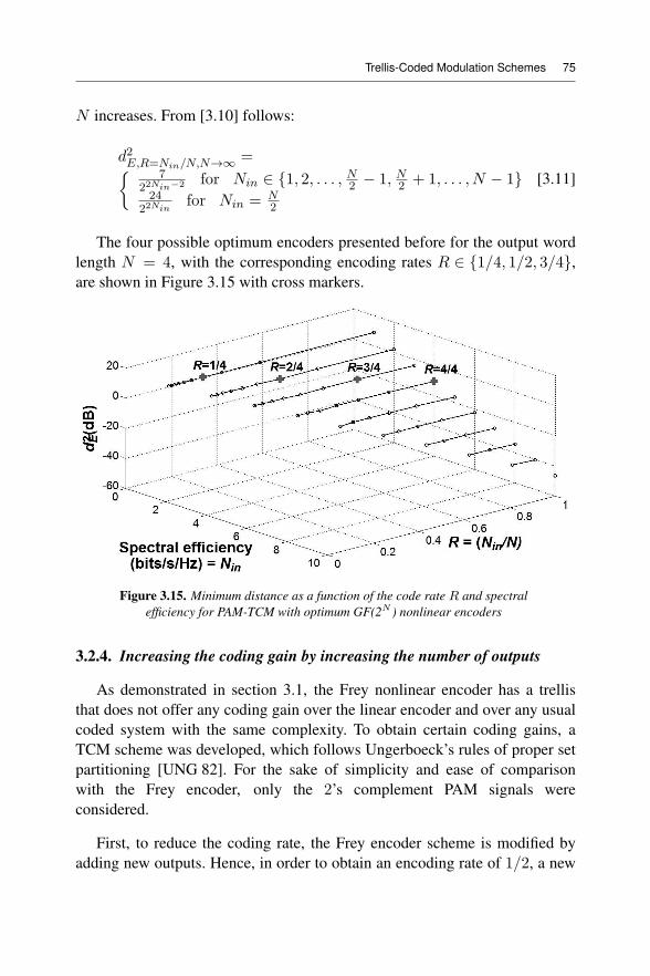
Trellis-Coded Modulation Schemes 75
N increases. From [3.10] follows:
d2E,R=Nin/N,N→∞ =7
22Nin−2 for Nin ∈ {1, 2, . . . , N2 − 1, N2 + 1, . . . , N − 1}24
22Ninfor Nin = N
2
[3.11]
The four possible optimum encoders presented before for the output wordlength N = 4, with the corresponding encoding rates R ∈ {1/4, 1/2, 3/4},are shown in Figure 3.15 with cross markers.
Figure 3.15. Minimum distance as a function of the code rate R and spectralefficiency for PAM-TCM with optimum GF(2N ) nonlinear encoders
3.2.4. Increasing the coding gain by increasing the number of outputs
As demonstrated in section 3.1, the Frey nonlinear encoder has a trellisthat does not offer any coding gain over the linear encoder and over any usualcoded system with the same complexity. To obtain certain coding gains, aTCM scheme was developed, which follows Ungerboeck’s rules of proper setpartitioning [UNG 82]. For the sake of simplicity and ease of comparisonwith the Frey encoder, only the 2’s complement PAM signals wereconsidered.
First, to reduce the coding rate, the Frey encoder scheme is modified byadding new outputs. Hence, in order to obtain an encoding rate of 1/2, a new
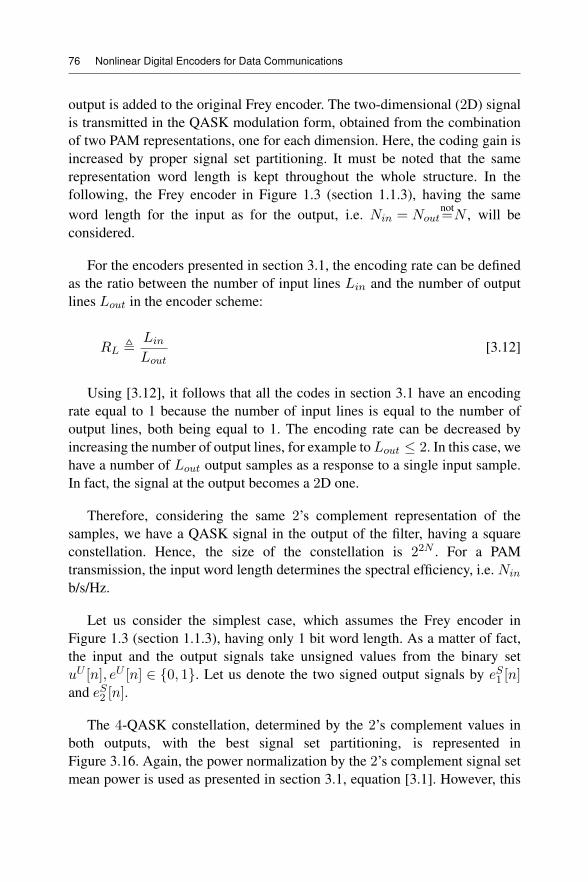
76 Nonlinear Digital Encoders for Data Communications
output is added to the original Frey encoder. The two-dimensional (2D) signalis transmitted in the QASK modulation form, obtained from the combinationof two PAM representations, one for each dimension. Here, the coding gain isincreased by proper signal set partitioning. It must be noted that the samerepresentation word length is kept throughout the whole structure. In thefollowing, the Frey encoder in Figure 1.3 (section 1.1.3), having the sameword length for the input as for the output, i.e. Nin = Nout
not=N , will be
considered.
For the encoders presented in section 3.1, the encoding rate can be definedas the ratio between the number of input lines Lin and the number of outputlines Lout in the encoder scheme:
RLLin
Lout[3.12]
Using [3.12], it follows that all the codes in section 3.1 have an encodingrate equal to 1 because the number of input lines is equal to the number ofoutput lines, both being equal to 1. The encoding rate can be decreased byincreasing the number of output lines, for example to Lout ≤ 2. In this case, wehave a number of Lout output samples as a response to a single input sample.In fact, the signal at the output becomes a 2D one.
Therefore, considering the same 2’s complement representation of thesamples, we have a QASK signal in the output of the filter, having a squareconstellation. Hence, the size of the constellation is 22N . For a PAMtransmission, the input word length determines the spectral efficiency, i.e. Nin
b/s/Hz.
Let us consider the simplest case, which assumes the Frey encoder inFigure 1.3 (section 1.1.3), having only 1 bit word length. As a matter of fact,the input and the output signals take unsigned values from the binary setuU [n], eU [n] ∈ {0, 1}. Let us denote the two signed output signals by eS1 [n]and eS2 [n].
The 4-QASK constellation, determined by the 2’s complement values inboth outputs, with the best signal set partitioning, is represented inFigure 3.16. Again, the power normalization by the 2’s complement signal setmean power is used as presented in section 3.1, equation [3.1]. However, this
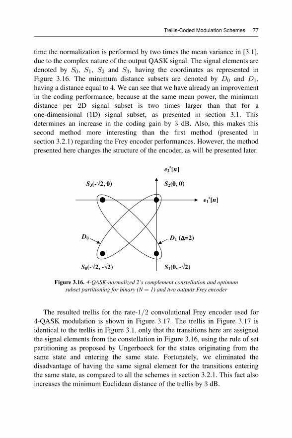
Trellis-Coded Modulation Schemes 77
time the normalization is performed by two times the mean variance in [3.1],due to the complex nature of the output QASK signal. The signal elements aredenoted by S0, S1, S2 and S3, having the coordinates as represented inFigure 3.16. The minimum distance subsets are denoted by D0 and D1,having a distance equal to 4. We can see that we have already an improvementin the coding performance, because at the same mean power, the minimumdistance per 2D signal subset is two times larger than that for aone-dimensional (1D) signal subset, as presented in section 3.1. Thisdetermines an increase in the coding gain by 3 dB. Also, this makes thissecond method more interesting than the first method (presented insection 3.2.1) regarding the Frey encoder performances. However, the methodpresented here changes the structure of the encoder, as will be presented later.
e1s[n]
e2s[n]
S2(0, 0)
D0 D1 (ΔΔΔΔ=2)
S3(- 2, 0)
S0(- 2, - 2) S1(0, - 2)
Figure 3.16. 4-QASK-normalized 2’s complement constellation and optimumsubset partitioning for binary (N = 1) and two outputs Frey encoder
The resulted trellis for the rate-1/2 convolutional Frey encoder used for4-QASK modulation is shown in Figure 3.17. The trellis in Figure 3.17 isidentical to the trellis in Figure 3.1, only that the transitions here are assignedthe signal elements from the constellation in Figure 3.16, using the rule of setpartitioning as proposed by Ungerboeck for the states originating from thesame state and entering the same state. Fortunately, we eliminated thedisadvantage of having the same signal element for the transitions enteringthe same state, as compared to all the schemes in section 3.2.1. This fact alsoincreases the minimum Euclidean distance of the trellis by 3 dB.
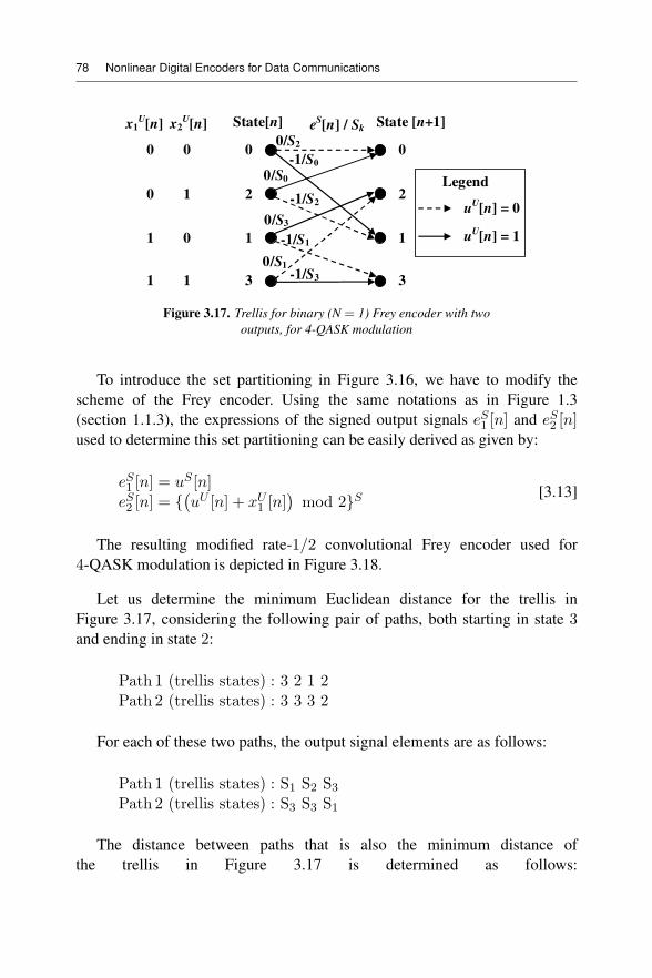
78 Nonlinear Digital Encoders for Data Communications
-1/S1
0/S3
0/S1
-1/S3
-1/S2
0/S0
-1/S0
0/S20 0
State[n]
0
0 1 2
1 0 1
1 1 3
State [n+1]
0
2
1
3
eS[n] / Sk
Legend
uU[n] = 0
uU[n] = 1
x1U[n] x2
U[n]
Figure 3.17. Trellis for binary (N = 1) Frey encoder with twooutputs, for 4-QASK modulation
To introduce the set partitioning in Figure 3.16, we have to modify thescheme of the Frey encoder. Using the same notations as in Figure 1.3(section 1.1.3), the expressions of the signed output signals eS1 [n] and eS2 [n]used to determine this set partitioning can be easily derived as given by:
eS1 [n] = uS [n]eS2 [n] = { uU [n] + xU1 [n] mod 2}S [3.13]
The resulting modified rate-1/2 convolutional Frey encoder used for4-QASK modulation is depicted in Figure 3.18.
Let us determine the minimum Euclidean distance for the trellis inFigure 3.17, considering the following pair of paths, both starting in state 3and ending in state 2:
Path 1 (trellis states) : 3 2 1 2Path 2 (trellis states) : 3 3 3 2
For each of these two paths, the output signal elements are as follows:
Path 1 (trellis states) : S1 S2 S3Path 2 (trellis states) : S3 S3 S1
The distance between paths that is also the minimum distance ofthe trellis in Figure 3.17 is determined as follows:
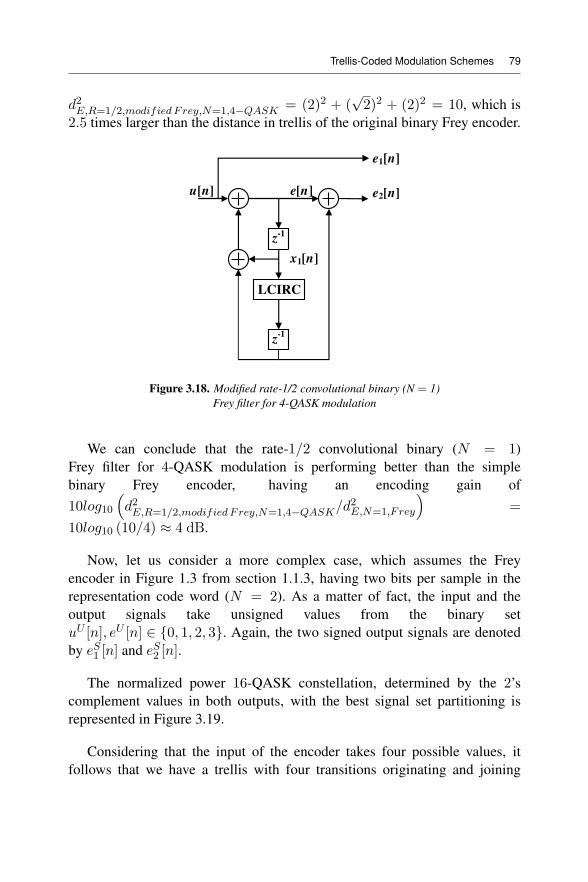
Trellis-Coded Modulation Schemes 79
d2E,R=1/2,modified Frey,N=1,4−QASK = (2)2 + (√2)2 + (2)2 = 10, which is
2.5 times larger than the distance in trellis of the original binary Frey encoder.
z-1
z-1
LCIRC
u[n] e[n]
x1[n]
e1[n]
e2[n]
Figure 3.18. Modified rate-1/2 convolutional binary (N = 1)Frey filter for 4-QASK modulation
We can conclude that the rate-1/2 convolutional binary (N = 1)Frey filter for 4-QASK modulation is performing better than the simplebinary Frey encoder, having an encoding gain of10log10 d2E,R=1/2,modified Frey,N=1,4−QASK/d2E,N=1,F rey =
10log10 (10/4) ≈ 4 dB.
Now, let us consider a more complex case, which assumes the Freyencoder in Figure 1.3 from section 1.1.3, having two bits per sample in therepresentation code word (N = 2). As a matter of fact, the input and theoutput signals take unsigned values from the binary setuU [n], eU [n] ∈ {0, 1, 2, 3}. Again, the two signed output signals are denotedby eS1 [n] and eS2 [n].
The normalized power 16-QASK constellation, determined by the 2’scomplement values in both outputs, with the best signal set partitioning isrepresented in Figure 3.19.
Considering that the input of the encoder takes four possible values, itfollows that we have a trellis with four transitions originating and joining
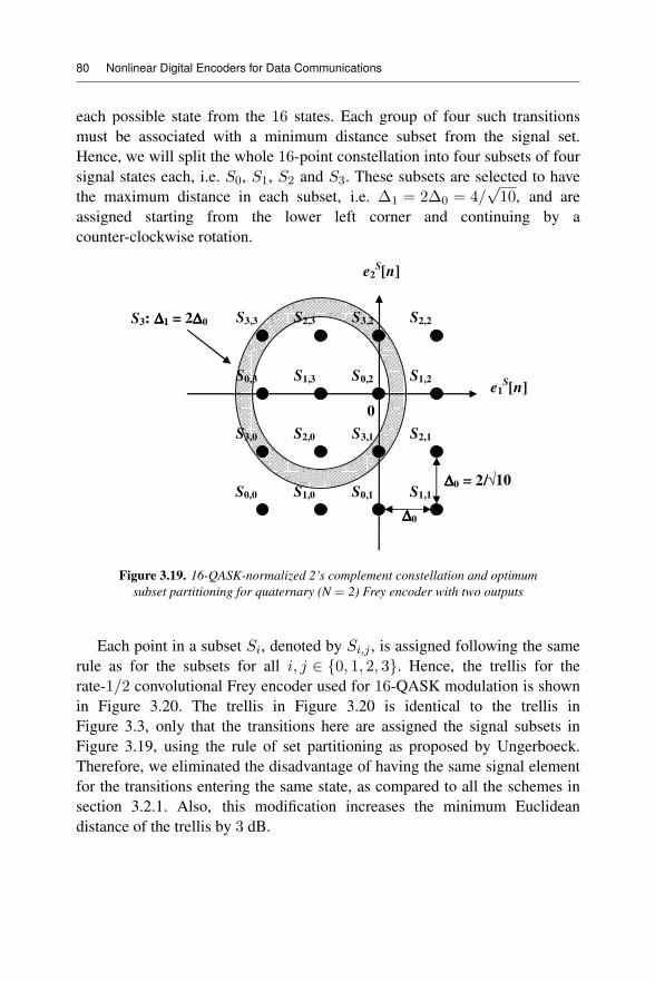
80 Nonlinear Digital Encoders for Data Communications
each possible state from the 16 states. Each group of four such transitionsmust be associated with a minimum distance subset from the signal set.Hence, we will split the whole 16-point constellation into four subsets of foursignal states each, i.e. S0, S1, S2 and S3. These subsets are selected to havethe maximum distance in each subset, i.e. Δ1 = 2Δ0 = 4/
√10, and are
assigned starting from the lower left corner and continuing by acounter-clockwise rotation.
e1S[n]
e2S[n]
S3: ΔΔΔΔ1 = 2ΔΔΔΔ0
ΔΔΔΔ0 = 2/ 10
ΔΔΔΔ0
S0,2
S0,1S0,0
S1,3 S1,2
S1,1S1,0
S2,3 S2,2
S2,1S2,0
S0,3
S3,3 S3,2
S3,1S3,0
0
Figure 3.19. 16-QASK-normalized 2’s complement constellation and optimumsubset partitioning for quaternary (N = 2) Frey encoder with two outputs
Each point in a subset Si, denoted by Si,j , is assigned following the samerule as for the subsets for all i, j ∈ {0, 1, 2, 3}. Hence, the trellis for therate-1/2 convolutional Frey encoder used for 16-QASK modulation is shownin Figure 3.20. The trellis in Figure 3.20 is identical to the trellis inFigure 3.3, only that the transitions here are assigned the signal subsets inFigure 3.19, using the rule of set partitioning as proposed by Ungerboeck.Therefore, we eliminated the disadvantage of having the same signal elementfor the transitions entering the same state, as compared to all the schemes insection 3.2.1. Also, this modification increases the minimum Euclideandistance of the trellis by 3 dB.
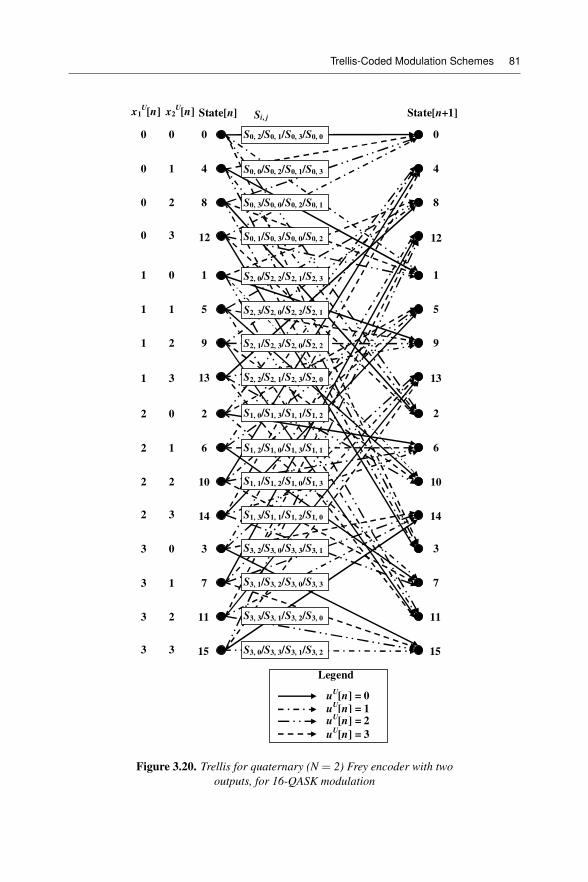
Trellis-Coded Modulation Schemes 81
0 0
State[n]
0
0 1 4
0 2 8
0 3 12
Legend
uU[n] = 0
uU[n] = 1
x1U[n] x2
U[n]
1 0 1
1 1 5
1 2 9
1 3 13
2 0 2
2 1 6
2 2 10
2 3
3 0 3
3 1 7
3 2
3 3
14
11
15
uU[n] = 2
uU[n] = 3
4
8
12
1
5
9
13
2
6
10
3
7
14
11
15
0
State[n+1]Si, j
S0, 0/S0, 2/S0, 1/S0, 3
S0, 3/S0, 0/S0, 2/S0, 1
S0, 1/S0, 3/S0, 0/S0, 2
S2, 0/S2, 2/S2, 1/S2, 3
S2, 3/S2, 0/S2, 2/S2, 1
S2, 1/S2, 3/S2, 0/S2, 2
S2, 2/S2, 1/S2, 3/S2, 0
S1, 0/S1, 3/S1, 1/S1, 2
S1, 2/S1, 0/S1, 3/S1, 1
S1, 1/S1, 2/S1, 0/S1, 3
S1, 3/S1, 1/S1, 2/S1, 0
S3, 2/S3, 0/S3, 3/S3, 1
S3, 1/S3, 2/S3, 0/S3, 3
S0, 2/S0, 1/S0, 3/S0, 0
S3, 3/S3, 1/S3, 2/S3, 0
S3, 0/S3, 3/S3, 1/S3, 2
Figure 3.20. Trellis for quaternary (N = 2) Frey encoder with twooutputs, for 16-QASK modulation
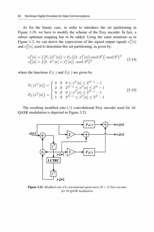
82 Nonlinear Digital Encoders for Data Communications
As for the binary case, in order to introduce the set partitioning inFigure 3.19, we have to modify the scheme of the Frey encoder. In fact, asubset optimum mapping has to be added. Using the same notations as inFigure 1.3, we can derive the expressions of the signed output signals eS1 [n]and eS2 [n], used to determine this set partitioning, as given by:
eS1 [n] = { F1 uU [n] + F2 3 · xU1 [n] mod 22 mod 22}SeS2 [n] = { 2 · uU [n] + xU1 [n] mod 22}S [3.14]
where the functions F1(.) and F2(.) are given by:
F1 xU [n] =0 if 0 ≤ xU [n] ≤ 2N−1 − 12 if 2N−1 ≤ xU [n] ≤ 2N − 1
F2 xU [n] =0 if 0 ≤ xU [n] ≤ 2N−1 − 11 if 2N−1 ≤ xU [n] ≤ 2N − 1
[3.15]
The resulting modified rate-1/2 convolutional Frey encoder used for 16-QASK modulation is depicted in Figure 3.21.
z-1
z-1
LCIRC
u[n]
x1[n]
x2[n]
e1[n]
e2[n]
F1(.)
F2(.)3
2
Figure 3.21. Modified rate-1/2 convolutional quaternary (N = 2) Frey encoderfor 16-QASK modulation
Trellis-Coded Modulation Schemes 83
We estimated the minimum Euclidean distance for the trellis in Figure 3.20,and we found two different values, each depending on the initial state in thetrellis. The following two examples will present these two cases.
First, let us consider the following pair of paths, both starting in state 0 andending in state 10:
Path 1 (trellis states) : 0 2 5 10Path 2 (trellis states) : 0 3 13 10
For these two paths, the output signal elements are the following:
Path 1 (trellis states) : S0,3 S1,3 S2,1Path 2 (trellis states) : S0,0 S3,0 S2,2
The distance between these two paths is:d2E,R=1/2,modified Frey,N=2,16−QASK = (2Δ0)
2 + Δ0
√2
2+ (2Δ0)
2 =
10Δ20 = 4, which is five times larger than the distance in trellis of the original
quaternary Frey encoder.
The second value of the Euclidean distance can be determined for pairs ofpaths as:
Path 1 (trellis states) : 1 11 14 4Path 2 (trellis states) : 1 8 2 4
For these two paths, the output signal elements are the following:
Path 1 (trellis states) : S2,3 S3,2 S1,3Path 2 (trellis states) : S2,0 S0,2 S1,0
The distance between these two paths is:d2E,R=1/2,modified Frey,N=2,16−QASK = (2Δ0)
2 + (Δ0)2 + (2Δ0)
2 = 9Δ20 =
3.6, which is 4.5 times larger than the distance in trellis of the originalquaternary Frey encoder.
84 Nonlinear Digital Encoders for Data Communications
In conclusion, the trellis in Figure 3.20 offers an encoding gain of at least10log10 d2E,R=1/2,modified Frey,N=2,16−QASK/d2E,N=2,F rey = 10log10
(3.6/0.8) ≈ 6.5dB over the simple quaternary Frey encoder.
The TCM design method presented earlier was also applied for Freyencoders with larger word lengths, but the complexity of such TCM schemesincreases dramatically. The number of trellis states grows exponentially withthe input word length, i.e. 22N . However, this trellis design method can begeneralized for any word length, determining in all cases significant encodinggains over the non-encoded system.
3.3. Optimum nonlinear encoders for phase shift keying – TCM schemes
3.3.1. Rate-1/2 optimum encoder for a QPSK-TCM transmission
In this section, the potential of the nonlinear LCIRC function is shown,for designing efficient encoders. Therefore, following the trellis optimizationpresented in [VLA 09a] and [VLA 09c], a simple nonlinear encoder operatingover GF (4) was developed, which has a binary input. It is demonstrated thatthis encoder performs identically to an optimum rate-1/2 binary field RSCconvolutional encoder. Both encoders offer maximum coding gain for 1 b/s/Hz[UNG 82, VLA 09a]. The scheme of the rate-1/2 optimum GF (4) encoderwas introduced in Figure 3.12. The same notations as in section 3.2.3 are used.The trellis for the encoder in Figure 3.12 is shown in Figure 3.13.
Mapping an unsigned output symbol value eU [n] into an instant carrierphase value ϕe[n] over the n-th sample interval, a 2N levels PSK-TCMscheme is obtained. A simple phase mapping is given by:
ϕe[n] = eU [n] · 2π2N
, eU [n] ∈ {0, 1, . . . 2N − 1} [3.16]
The phase constellation for the QPSK scheme using the mapping in [3.16]is represented in Figure 3.22.
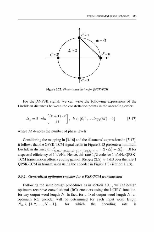
Trellis-Coded Modulation Schemes 85
eU
= 0
ΔΔΔΔ1 = 2
eU
= 1
eU
= 2
eU
= 3
ΔΔΔΔ0 = 2
Figure 3.22. Phase constellation for QPSK-TCM
For the M -PSK signal, we can write the following expressions of theEuclidean distances between the constellation points in the ascending order:
Δk = 2 · sin (k + 1) · πM
, k ∈ {0, 1, . . . log2(M)− 1} [3.17]
where M denotes the number of phase levels.
Considering the mapping in [3.16] and the distances’ expressions in [3.17],it follows that the QPSK-TCM signal trellis in Figure 3.13 presents a minimumEuclidean distance of d2
E,R=1/2,opt.,uU [n]∈{0,2},QPSK= 2 ·Δ2
1 +Δ20 = 10 for
a spectral efficiency of 1 b/s/Hz. Hence, this rate-1/2 code for 1 b/s/Hz QPSK-TCM transmission offers a coding gain of 10log10 (2.5) ≈ 4 dB over the rate-1QPSK-TCM in transmission using the encoder in Figure 1.3 (section 1.1.3).
3.3.2. Generalized optimum encoder for a PSK-TCM transmission
Following the same design procedures as in section 3.3.1, we can designoptimum recursive convolutional (RC) encoders using the LCIRC function,for any output word length N . In fact, for a fixed output word length N , anoptimum RC encoder will be determined for each input word lengthNin ∈ {1, 2, . . . , N − 1}, for which the encoding rate is
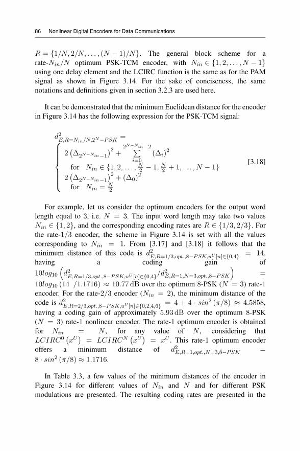
86 Nonlinear Digital Encoders for Data Communications
R = {1/N, 2/N, . . . , (N − 1)/N}. The general block scheme for arate-Nin/N optimum PSK-TCM encoder, with Nin ∈ {1, 2, . . . , N − 1}using one delay element and the LCIRC function is the same as for the PAMsignal as shown in Figure 3.14. For the sake of conciseness, the samenotations and definitions given in section 3.2.3 are used here.
It can be demonstrated that the minimum Euclidean distance for the encoderin Figure 3.14 has the following expression for the PSK-TCM signal:
d2E,R=Nin/N,2N−PSK
=⎧⎪⎪⎪⎪⎪⎨⎪⎪⎪⎪⎪⎩2 Δ2N−Nin−1
2+
2N−Nin−2
i=0(Δi)
2
for Nin ∈ {1, 2, . . . , N2 − 1, N2 + 1, . . . , N − 1}2 Δ2N−Nin−1
2+ (Δ0)
2
for Nin = N2
[3.18]
For example, let us consider the optimum encoders for the output wordlength equal to 3, i.e. N = 3. The input word length may take two valuesNin ∈ {1, 2}, and the corresponding encoding rates are R ∈ {1/3, 2/3}. Forthe rate-1/3 encoder, the scheme in Figure 3.14 is set with all the valuescorresponding to Nin = 1. From [3.17] and [3.18] it follows that theminimum distance of this code is d2
E,R=1/3,opt.,8−PSK,uU [n]∈{0,4} = 14,having a coding gain of10log10 d2
E,R=1/3,opt.,8−PSK,uU [n]∈{0,4}/d2E,R=1,N=3,opt.,8−PSK =
10log10 (14 /1.1716) ≈ 10.77 dB over the optimum 8-PSK (N = 3) rate-1encoder. For the rate-2/3 encoder (Nin = 2), the minimum distance of thecode is d2
E,R=2/3,opt.,8−PSK,uU [n]∈{0,2,4,6} = 4 + 4 · sin2 (π/8) ≈ 4.5858,having a coding gain of approximately 5.93 dB over the optimum 8-PSK(N = 3) rate-1 nonlinear encoder. The rate-1 optimum encoder is obtainedfor Nin = N , for any value of N , considering thatLCIRC0 xU = LCIRCN xU = xU . This rate-1 optimum encoderoffers a minimum distance of d2E,R=1,opt.,N=3,8−PSK =
8 · sin2 (π/8) ≈ 1.1716.
In Table 3.3, a few values of the minimum distances of the encoder inFigure 3.14 for different values of Nin and N and for different PSKmodulations are presented. The resulting coding rates are presented in the
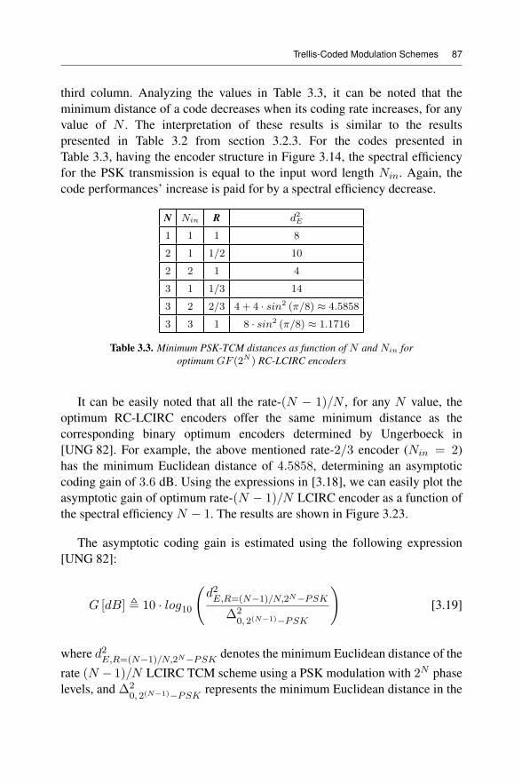
Trellis-Coded Modulation Schemes 87
third column. Analyzing the values in Table 3.3, it can be noted that theminimum distance of a code decreases when its coding rate increases, for anyvalue of N . The interpretation of these results is similar to the resultspresented in Table 3.2 from section 3.2.3. For the codes presented inTable 3.3, having the encoder structure in Figure 3.14, the spectral efficiencyfor the PSK transmission is equal to the input word length Nin. Again, thecode performances’ increase is paid for by a spectral efficiency decrease.
N Nin R d2E
1 1 1 8
2 1 1/2 10
2 2 1 4
3 1 1/3 14
3 2 2/3 4 + 4 · sin2 (π/8) ≈ 4.5858
3 3 1 8 · sin2 (π/8) ≈ 1.1716
Table 3.3. Minimum PSK-TCM distances as function of N and Nin foroptimum GF (2N ) RC-LCIRC encoders
It can be easily noted that all the rate-(N − 1)/N , for any N value, theoptimum RC-LCIRC encoders offer the same minimum distance as thecorresponding binary optimum encoders determined by Ungerboeck in[UNG 82]. For example, the above mentioned rate-2/3 encoder (Nin = 2)has the minimum Euclidean distance of 4.5858, determining an asymptoticcoding gain of 3.6 dB. Using the expressions in [3.18], we can easily plot theasymptotic gain of optimum rate-(N − 1)/N LCIRC encoder as a function ofthe spectral efficiency N − 1. The results are shown in Figure 3.23.
The asymptotic coding gain is estimated using the following expression[UNG 82]:
G [dB] 10 · log10d2E,R=(N−1)/N,2N−PSK
Δ20, 2(N−1)−PSK
[3.19]
where d2E,R=(N−1)/N,2N−PSK
denotes the minimum Euclidean distance of the
rate (N − 1)/N LCIRC TCM scheme using a PSK modulation with 2N phaselevels, and Δ2
0, 2(N−1)−PSKrepresents the minimum Euclidean distance in the
88 Nonlinear Digital Encoders for Data Communications
2(N−1)-PSK non-coded signal constellation. Hence, the asymptotic coded gainspecifies the gain of the coded scheme when doubling the signal constellationsize over the non-coded signal. As shown in Figure 3.23, the asymptotic gaindecays rapidly to a limit value when the number of signal levels increases. Thislimit specifies the maximum number of signal levels to be selected.
0 2 4 6 8 103.5
3.55
3.6
3.65
3.7
3.75
3.8
3.85
3.9
3.95
4
←R=2/3 (Coded 8-PSK)
↓G∞∞∞∞ = 3.5218
Spectral efficiency (bits/s/Hz) = Nin = N - 1
Asym
pto
tic
Co
din
gG
ain
,G
(dB
)
Figure 3.23. Asymptotic gain as a function of the spectral efficiency for rate(N − 1)/N optimum GF(2N ) recursive convolutional LCIRC encoders
However, the GF (2N ) optimum RC-LCIRC encoders are less complexthan the corresponding binary encoders. The memory size of the binaryencoders increases logarithmically with the number of states in the trellis,while the GF (2N ) optimum RC-LCIRC encoders include only one delayelement, irrespective of the trellis complexity. As another advantage of theseencoders, we can also mention the Euclidean distance compact expression asa function of Nin and N .
All TCM schemes presented earlier used PSK modulation. Even if PSK isused in practice only for small spectral efficiencies, i.e. up to 3 b/s/Hz,optimum RC-LCIRC encoders can be designed for any spectral efficiencyvalue, using the scheme in Figure 3.14 with minimum distances given by[3.17] and [3.18].
Trellis-Coded Modulation Schemes 89
3.4. Optimum nonlinear encoders for quadrature amplitude modulation– TCM schemes
Following the same design procedures as in section 3.3.2, we can designoptimum RC encoders for quadrature amplitude modulation TCM(QAM-TCM) schemes using the LCIRC function having any value for theoutput word length N . Let us consider the general block scheme for arate-Nin/N optimum QAM-TCM encoder, with Nin ∈ {1, 2, . . . , N − 1}using one delay element and the LCIRC function, which is shown inFigure 3.14. For the sake of conciseness, all notations and definitions given insection 3.2.3 are kept here.
It can be demonstrated that the minimum Euclidean distance for the encoderin Figure 3.14 has the following expression for the QAM-TCM signal:
d2E,R=Nin/N,2N−QAM
=⎧⎪⎪⎪⎪⎪⎨⎪⎪⎪⎪⎪⎩2N−Nin+1 +
N−Nin−1
i=02i ·Δ2
0, 2N−QAM
for Nin ∈ {1, 2, . . . , N2 − 1, N2 + 1, . . . , N − 1}2N−Nin+1 + 1 ·Δ2
0, 2N−QAM
for Nin = N2
[3.20]
For example, let us consider the optimum encoders for the output wordlength equal to 4, i.e. N = 4. The input word length may take three valuesNin ∈ {1, 2, 3}, and the corresponding encoding rates areR ∈ {1/4, 1/2, 3/4}. For the rate-1/4 encoder, the scheme in Figure 3.14 isset with all the values corresponding to Nin = 1. From [3.20], it follows thatthe minimum distance of this code is d2
E,R=1/4,opt.,16−QAM,uU [n]∈{0,8} = 9.2,
determining a coding gain of 10log10 d2E,R=1/4,opt.,16−QAM,uU [n]∈{0,8}
/ d2E,R=1,N=4,opt.,16−QAM = 10log10 (9.2/0.8) ≈ 10.6 dB over theoptimum 16-QAM (N = 4) rate-1 encoder. For the rate-2/4 encoder(Nin = 2), the minimum distance of the code isd2E,R=1/2,opt.,16−QAM,uU [n]∈{0,4,8,12} = 3.6, having a coding gain of
approximately 6.53 dB over the optimum 16-QAM (N = 4) rate-1 nonlinearencoder. For the rate-3/4 encoder (Nin = 3), the minimum distance of thecode is d2
E,R=3/4,opt.,16−QAM,uU [n]∈{0,2,4,6,8,10,12,14} = 2, having a codinggain of approximately 3.97 dB over the optimum 16-QAM (N = 4) rate-1
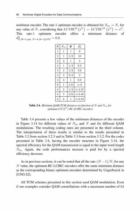
90 Nonlinear Digital Encoders for Data Communications
nonlinear encoder. The rate-1 optimum encoder is obtained for Nin = N , forany value of N , considering that LCIRC0 xU = LCIRCN xU = xU .This rate-1 optimum encoder offers a minimum distance ofd2E,R=1,opt.,N=4,16−QAM = 0.8.
N Nin R d2E
1 1 1 8
2 1 1/2 10
2 2 1 4
4 1 1/4 9.2
4 2 1/2 3.6
4 3 3/4 2
4 4 1 0.8
6 1 1/6 ≈ 9
6 2 1/3 ≈ 4.47
6 5 5/6 ≈ 0.48
6 6 1 ≈ 0.19
Table 3.4. Minimum QAM-TCM distances as function of N and Nin foroptimum GF (2N ) RC-LCIRC encoders
Table 3.4 presents a few values of the minimum distances of the encoderin Figure 3.14 for different values of Nin and N and for different QAMmodulations. The resulting coding rates are presented in the third column.The interpretation of these results is similar to the results presented inTable 3.2 from section 3.2.3 and in Table 3.3 from section 3.3.2. For the codespresented in Table 3.4, having the encoder structure in Figure 3.14, thespectral efficiency for the QAM transmission is equal to the input word lengthNin. Again, the code performances increase is paid for by a spectralefficiency decrease.
As in previous sections, it can be noted that all the rate-(N −1)/N , for anyN value, the optimum RC-LCIRC encoders offer the same minimum distanceas the corresponding binary optimum encoders determined by Ungerboeck in[UNG 82].
All TCM schemes presented in this section used QAM modulation. Evenif our examples consider QAM constellations with a maximum number of 64
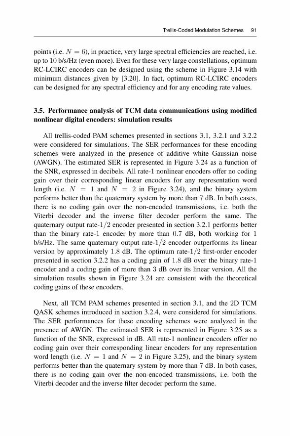
Trellis-Coded Modulation Schemes 91
points (i.e. N = 6), in practice, very large spectral efficiencies are reached, i.e.up to 10 b/s/Hz (even more). Even for these very large constellations, optimumRC-LCIRC encoders can be designed using the scheme in Figure 3.14 withminimum distances given by [3.20]. In fact, optimum RC-LCIRC encoderscan be designed for any spectral efficiency and for any encoding rate values.
3.5. Performance analysis of TCM data communications using modifiednonlinear digital encoders: simulation results
All trellis-coded PAM schemes presented in sections 3.1, 3.2.1 and 3.2.2were considered for simulations. The SER performances for these encodingschemes were analyzed in the presence of additive white Gaussian noise(AWGN). The estimated SER is represented in Figure 3.24 as a function ofthe SNR, expressed in decibels. All rate-1 nonlinear encoders offer no codinggain over their corresponding linear encoders for any representation wordlength (i.e. N = 1 and N = 2 in Figure 3.24), and the binary systemperforms better than the quaternary system by more than 7 dB. In both cases,there is no coding gain over the non-encoded transmissions, i.e. both theViterbi decoder and the inverse filter decoder perform the same. Thequaternary output rate-1/2 encoder presented in section 3.2.1 performs betterthan the binary rate-1 encoder by more than 0.7 dB, both working for 1b/s/Hz. The same quaternary output rate-1/2 encoder outperforms its linearversion by approximately 1.8 dB. The optimum rate-1/2 first-order encoderpresented in section 3.2.2 has a coding gain of 1.8 dB over the binary rate-1encoder and a coding gain of more than 3 dB over its linear version. All thesimulation results shown in Figure 3.24 are consistent with the theoreticalcoding gains of these encoders.
Next, all TCM PAM schemes presented in section 3.1, and the 2D TCMQASK schemes introduced in section 3.2.4, were considered for simulations.The SER performances for these encoding schemes were analyzed in thepresence of AWGN. The estimated SER is represented in Figure 3.25 as afunction of the SNR, expressed in dB. All rate-1 nonlinear encoders offer nocoding gain over their corresponding linear encoders for any representationword length (i.e. N = 1 and N = 2 in Figure 3.25), and the binary systemperforms better than the quaternary system by more than 7 dB. In both cases,there is no coding gain over the non-encoded transmissions, i.e. both theViterbi decoder and the inverse filter decoder perform the same.
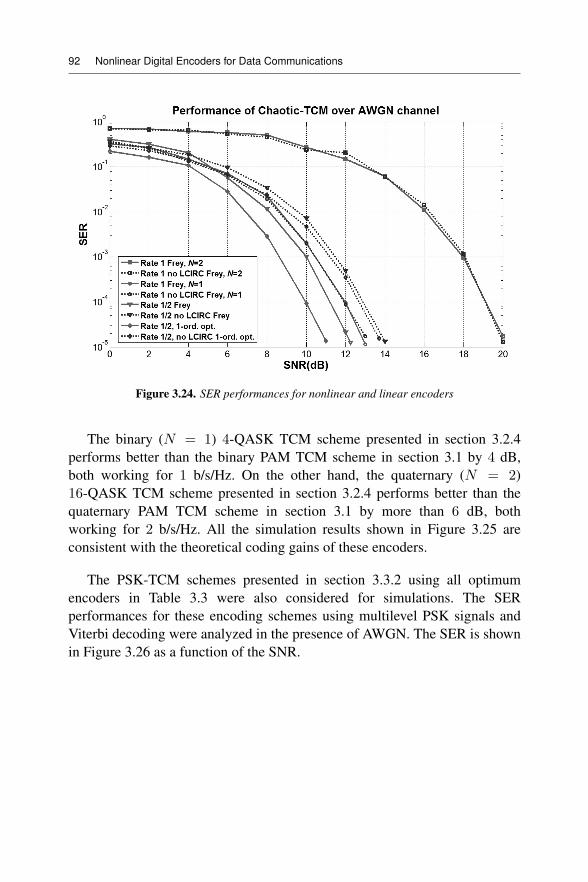
92 Nonlinear Digital Encoders for Data Communications
Figure 3.24. SER performances for nonlinear and linear encoders
The binary (N = 1) 4-QASK TCM scheme presented in section 3.2.4performs better than the binary PAM TCM scheme in section 3.1 by 4 dB,both working for 1 b/s/Hz. On the other hand, the quaternary (N = 2)16-QASK TCM scheme presented in section 3.2.4 performs better than thequaternary PAM TCM scheme in section 3.1 by more than 6 dB, bothworking for 2 b/s/Hz. All the simulation results shown in Figure 3.25 areconsistent with the theoretical coding gains of these encoders.
The PSK-TCM schemes presented in section 3.3.2 using all optimumencoders in Table 3.3 were also considered for simulations. The SERperformances for these encoding schemes using multilevel PSK signals andViterbi decoding were analyzed in the presence of AWGN. The SER is shownin Figure 3.26 as a function of the SNR.
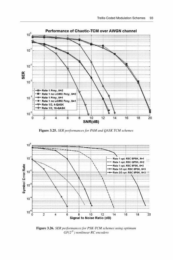
Trellis-Coded Modulation Schemes 93
Figure 3.25. SER performances for PAM and QASK TCM schemes
Figure 3.26. SER performances for PSK-TCM schemes using optimumGF(2N ) nonlinear RC encoders
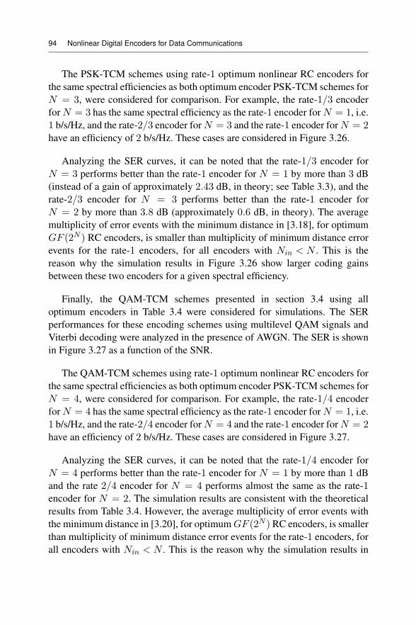
94 Nonlinear Digital Encoders for Data Communications
The PSK-TCM schemes using rate-1 optimum nonlinear RC encoders forthe same spectral efficiencies as both optimum encoder PSK-TCM schemes forN = 3, were considered for comparison. For example, the rate-1/3 encoderfor N = 3 has the same spectral efficiency as the rate-1 encoder for N = 1, i.e.1 b/s/Hz, and the rate-2/3 encoder for N = 3 and the rate-1 encoder for N = 2have an efficiency of 2 b/s/Hz. These cases are considered in Figure 3.26.
Analyzing the SER curves, it can be noted that the rate-1/3 encoder forN = 3 performs better than the rate-1 encoder for N = 1 by more than 3 dB(instead of a gain of approximately 2.43 dB, in theory; see Table 3.3), and therate-2/3 encoder for N = 3 performs better than the rate-1 encoder forN = 2 by more than 3.8 dB (approximately 0.6 dB, in theory). The averagemultiplicity of error events with the minimum distance in [3.18], for optimumGF (2N ) RC encoders, is smaller than multiplicity of minimum distance errorevents for the rate-1 encoders, for all encoders with Nin < N . This is thereason why the simulation results in Figure 3.26 show larger coding gainsbetween these two encoders for a given spectral efficiency.
Finally, the QAM-TCM schemes presented in section 3.4 using alloptimum encoders in Table 3.4 were considered for simulations. The SERperformances for these encoding schemes using multilevel QAM signals andViterbi decoding were analyzed in the presence of AWGN. The SER is shownin Figure 3.27 as a function of the SNR.
The QAM-TCM schemes using rate-1 optimum nonlinear RC encoders forthe same spectral efficiencies as both optimum encoder PSK-TCM schemes forN = 4, were considered for comparison. For example, the rate-1/4 encoderfor N = 4 has the same spectral efficiency as the rate-1 encoder for N = 1, i.e.1 b/s/Hz, and the rate-2/4 encoder for N = 4 and the rate-1 encoder for N = 2have an efficiency of 2 b/s/Hz. These cases are considered in Figure 3.27.
Analyzing the SER curves, it can be noted that the rate-1/4 encoder forN = 4 performs better than the rate-1 encoder for N = 1 by more than 1 dBand the rate 2/4 encoder for N = 4 performs almost the same as the rate-1encoder for N = 2. The simulation results are consistent with the theoreticalresults from Table 3.4. However, the average multiplicity of error events withthe minimum distance in [3.20], for optimum GF (2N ) RC encoders, is smallerthan multiplicity of minimum distance error events for the rate-1 encoders, forall encoders with Nin < N . This is the reason why the simulation results in
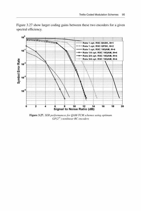
Trellis-Coded Modulation Schemes 95
Figure 3.27 show larger coding gains between these two encoders for a givenspectral efficiency.
Figure 3.27. SER performances for QAM-TCM schemes using optimumGF(2N ) nonlinear RC encoders

4
Parallel Turbo Trellis-Coded ModulationSchemes Using Nonlinear Digital
Encoders
4.1. Recursive convolutional-left circulate (RC-LCIRC) encoder in aturbo trellis-coded modulation (TTCM) scheme
Figure 4.1 shows the parallel turbo trellis-coded modulation (TTCM)encoder for 2N -phase shift keying (PSK) modulation. The informationsequence and the Nin bits blockwise interleaved sequence are fed intocomponent encoders recursive convolutional-left circulate 1 (RC-LCIRC1)and RC-LCIRC2 of rate Nin/N , shown in Figure 3.14, and mapped into2N -PSK or 2N -quadrature amplitude modulation (QAM) symbol sequence(x[n]). The non-systematic nature of the RC-LCIRC encoder does not permitthe parity bits puncturing as in traditional TTCM schemes. Hence, the overallcoding rate for the scheme in Figure 4.1 is Nin/(2 ·N). The 2N -PSK symbolsequence is transmitted over a noisy channel. The received signal over the nthsymbol interval is given by:
y[n] = x[n] + w[n] [4.1]
where w[n] is an additive white Gaussian noise (AWGN) sequence and x[n]denotes the 2N -PSK symbol sequence mapped from the encoder outputsequence {eU1 [n], eU2 [n]}; here, {eU [n]} denotes the output of the componentRC-LCIRC encoder, as presented in section 3.2.3.
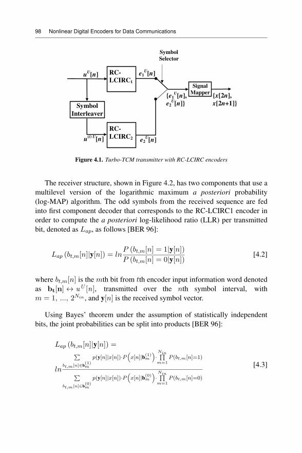
98 Nonlinear Digital Encoders for Data Communications
e1U[n]
e2U[n]u
(i) U[n]
uU[n] RC-
LCIRC1Signal
Mapper
RC-
LCIRC2
Symbol
Interleaver
Symbol
Selector
{x[2n],
x[2n+1]}
{e1U[n],
e2U[n]}
Figure 4.1. Turbo-TCM transmitter with RC-LCIRC encoders
The receiver structure, shown in Figure 4.2, has two components that use amultilevel version of the logarithmic maximum a posteriori probability(log-MAP) algorithm. The odd symbols from the received sequence are fedinto first component decoder that corresponds to the RC-LCIRC1 encoder inorder to compute the a posteriori log-likelihood ratio (LLR) per transmittedbit, denoted as Lap, as follows [BER 96]:
Lap (bt,m[n]|y[n]) = lnP (bt,m[n] = 1|y[n])P (bt,m[n] = 0|y[n]) [4.2]
where bt,m[n] is the mth bit from tth encoder input information word denotedas bt[n] ↔ uU [n], transmitted over the nth symbol interval, withm = 1, ..., 2Nin , and y[n] is the received symbol vector.
Using Bayes’ theorem under the assumption of statistically independentbits, the joint probabilities can be split into products [BER 96]:
Lap (bt,m[n]|y[n]) =
lnbt,m[n]∈b(1)m
p(y[n]|x[n])·P x[n]|b(1)m ·
Nin
m=1P (bt,m[n]=1)
bt,m[n]∈b(0)m
p(y[n]|x[n])·P x[n]|b(0)m ·
Nin
m=1P (bt,m[n]=0)
[4.3]
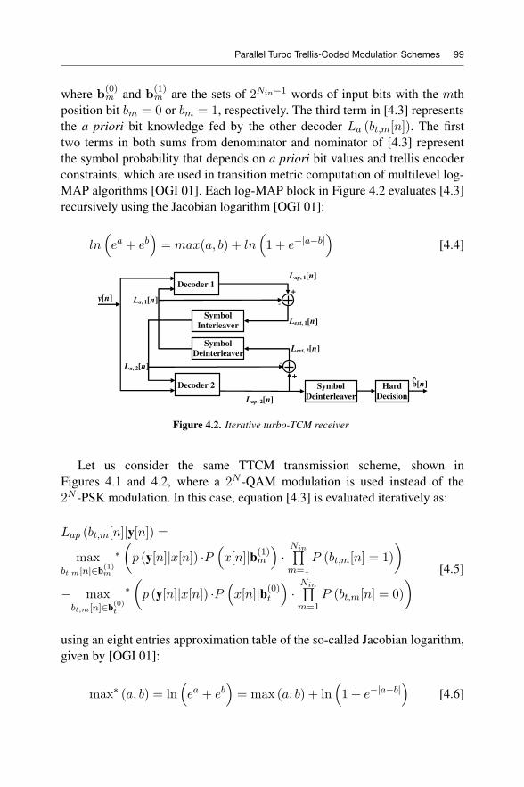
Parallel Turbo Trellis-Coded Modulation Schemes 99
where b(0)m and b
(1)m are the sets of 2Nin−1 words of input bits with the mth
position bit bm = 0 or bm = 1, respectively. The third term in [4.3] representsthe a priori bit knowledge fed by the other decoder La (bt,m[n]). The firsttwo terms in both sums from denominator and nominator of [4.3] representthe symbol probability that depends on a priori bit values and trellis encoderconstraints, which are used in transition metric computation of multilevel log-MAP algorithms [OGI 01]. Each log-MAP block in Figure 4.2 evaluates [4.3]recursively using the Jacobian logarithm [OGI 01]:
ln ea + eb = max(a, b) + ln 1 + e−|a−b| [4.4]
y[n]
Lap, 1[n]
La, 2[n]
Lext, 2[n]
Lext, 1[n]
Symbol
Deinterleaver
Decoder 2
Symbol
Deinterleaver
Decoder 1
Lap, 2[n]
Hard
Decision
La, 1[n]+
-
Symbol
Interleaver
+
-
b[n]^
Figure 4.2. Iterative turbo-TCM receiver
Let us consider the same TTCM transmission scheme, shown inFigures 4.1 and 4.2, where a 2N -QAM modulation is used instead of the2N -PSK modulation. In this case, equation [4.3] is evaluated iteratively as:
Lap (bt,m[n]|y[n]) =max
bt,m[n]∈b(1)m
∗ p (y[n]|x[n]) ·P x[n]|b(1)m ·
Nin
m=1P (bt,m[n] = 1)
− maxbt,m[n]∈b(0)
t
∗ p (y[n]|x[n]) ·P x[n]|b(0)t ·
Nin
m=1P (bt,m[n] = 0)
[4.5]
using an eight entries approximation table of the so-called Jacobian logarithm,given by [OGI 01]:
max∗ (a, b) = ln ea + eb = max (a, b) + ln 1 + e−|a−b| [4.6]
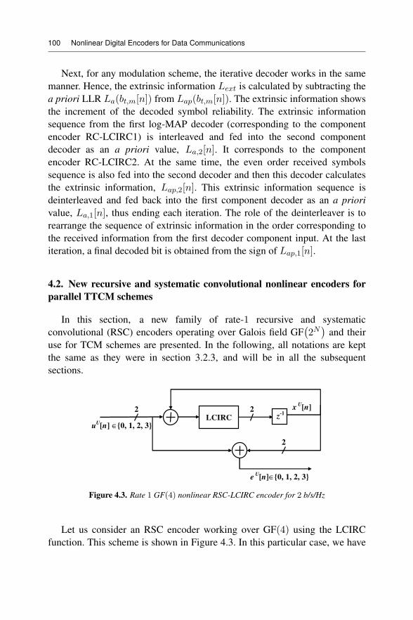
100 Nonlinear Digital Encoders for Data Communications
Next, for any modulation scheme, the iterative decoder works in the samemanner. Hence, the extrinsic information Lext is calculated by subtracting thea priori LLR La(bt,m[n]) from Lap(bt,m[n]). The extrinsic information showsthe increment of the decoded symbol reliability. The extrinsic informationsequence from the first log-MAP decoder (corresponding to the componentencoder RC-LCIRC1) is interleaved and fed into the second componentdecoder as an a priori value, La,2[n]. It corresponds to the componentencoder RC-LCIRC2. At the same time, the even order received symbolssequence is also fed into the second decoder and then this decoder calculatesthe extrinsic information, Lap,2[n]. This extrinsic information sequence isdeinterleaved and fed back into the first component decoder as an a priorivalue, La,1[n], thus ending each iteration. The role of the deinterleaver is torearrange the sequence of extrinsic information in the order corresponding tothe received information from the first decoder component input. At the lastiteration, a final decoded bit is obtained from the sign of Lap,1[n].
4.2. New recursive and systematic convolutional nonlinear encoders forparallel TTCM schemes
In this section, a new family of rate-1 recursive and systematicconvolutional (RSC) encoders operating over Galois field GF 2N and theiruse for TCM schemes are presented. In the following, all notations are keptthe same as they were in section 3.2.3, and will be in all the subsequentsections.
uU[n] ∈{0, 1, 2, 3}
z-1
LCIRC
xU[n]2 2
eU[n]∈{0, 1, 2, 3}
2
Figure 4.3. Rate 1 GF(4) nonlinear RSC-LCIRC encoder for 2 b/s/Hz
Let us consider an RSC encoder working over GF(4) using the LCIRCfunction. This scheme is shown in Figure 4.3. In this particular case, we have
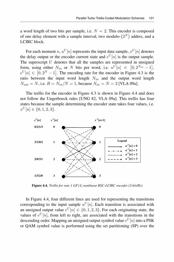
Parallel Turbo Trellis-Coded Modulation Schemes 101
a word length of two bits per sample, i.e. N = 2. This encoder is composedof one delay element with a sample interval, two modulo- 2N adders, and aLCIRC block.
For each moment n, uU [n] represents the input data sample, xU [n] denotesthe delay output or the encoder current state and eU [n] is the output sample.The superscript U denotes that all the samples are represented in unsignedform, using either Nin or N bits per word, i.e. uU [n] ∈ 0, 2Nin − 1 ,eU [n] ∈ 0, 2N − 1 . The encoding rate for the encoder in Figure 4.3 is theratio between the input word length Nin and the output word lengthNout = N , i.e. R = Nin/N = 1, because Nin = N = 2 [VLA 09a].
The trellis for the encoder in Figure 4.3 is shown in Figure 4.4 and doesnot follow the Ungerboeck rules [UNG 82, VLA 09a]. This trellis has fourstates because the sample determining the encoder state takes four values, i.e.xU [n] ∈ {0, 1, 2, 3}.
0/2/1/3 0
1
2
3
0
1
2
3
eU[n] x
U[n] x
U[n+1]
Legend
uU[n] = 0
uU[n] = 1
uU[n] = 2
uU[n] = 3
3/1/0/2
2/0/3/1
1/3/2/0
Figure 4.4. Trellis for rate 1 GF(4) nonlinear RSC-LCIRC encoder (2 b/s/Hz)
In Figure 4.4, four different lines are used for representing the transitionscorresponding to the input sample uU [n]. Each transition is associated withan unsigned output value eU [n] ∈ {0, 1, 2, 3}. For each originating state, thevalues of eU [n], from left to right, are associated with the transitions in thedescending order. Mapping an unsigned output symbol value eU [n] into a PSKor QAM symbol value is performed using the set partitioning (SP) over the
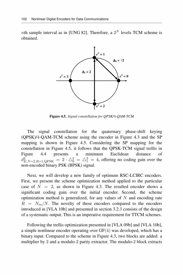
102 Nonlinear Digital Encoders for Data Communications
nth sample interval as in [UNG 82]. Therefore, a 2N levels TCM scheme isobtained.
eU
= 0
ΔΔΔΔ1 = 2
eU
= 1
eU
= 3
eU
= 2
ΔΔΔΔ0 = 2
Figure 4.5. Signal constellation for QPSK/4-QAM-TCM
The signal constellation for the quaternary phase-shift keying(QPSK)/4-QAM-TCM scheme using the encoder in Figure 4.3 and the SPmapping is shown in Figure 4.5. Considering the SP mapping for theconstellation in Figure 4.5, it follows that the QPSK-TCM signal trellis inFigure 4.4 presents a minimum Euclidean distance ofd2E,N=2,R=1,QPSK = 2 · 2
0 = 21 = 4, offering no coding gain over the
non-encoded binary PSK (BPSK) signal.
Next, we will develop a new family of optimum RSC-LCIRC encoders.First, we present the scheme optimization method applied to the particularcase of N = 2, as shown in Figure 4.3. The resulted encoder shows asignificant coding gain over the initial encoder. Second, the schemeoptimization method is generalized, for any values of N and encoding rateR = Nin/N . The novelty of these encoders compared to the encodersintroduced in [VLA 10b] and presented in section 3.2.3 consists of the designof a systematic output. This is an imperative requirement for TTCM schemes.
Following the trellis optimization presented in [VLA 09b] and [VLA 10b],a simple nonlinear encoder operating over GF(4) was developed, which has abinary input. Compared to the scheme in Figure 4.3, two blocks are added: amultiplier by 2 and a modulo-2 parity extractor. The modulo-2 block extracts
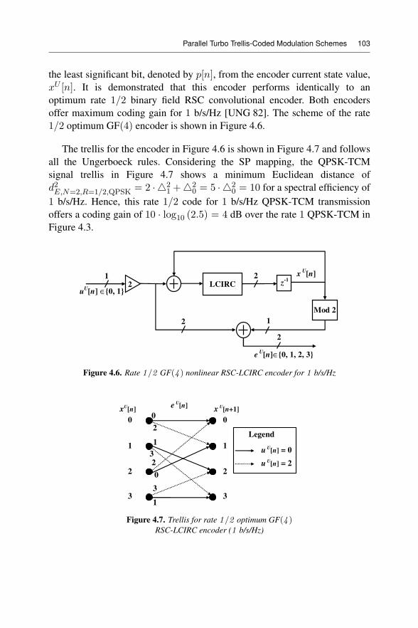
Parallel Turbo Trellis-Coded Modulation Schemes 103
the least significant bit, denoted by p[n], from the encoder current state value,xU [n]. It is demonstrated that this encoder performs identically to anoptimum rate 1/2 binary field RSC convolutional encoder. Both encodersoffer maximum coding gain for 1 b/s/Hz [UNG 82]. The scheme of the rate1/2 optimum GF(4) encoder is shown in Figure 4.6.
The trellis for the encoder in Figure 4.6 is shown in Figure 4.7 and followsall the Ungerboeck rules. Considering the SP mapping, the QPSK-TCMsignal trellis in Figure 4.7 shows a minimum Euclidean distance ofd2E,N=2,R=1/2,QPSK = 2 · 2
1 +20 = 5 · 2
0 = 10 for a spectral efficiency of1 b/s/Hz. Hence, this rate 1/2 code for 1 b/s/Hz QPSK-TCM transmissionoffers a coding gain of 10 · log10 (2.5) = 4 dB over the rate 1 QPSK-TCM inFigure 4.3.
uU[n] ∈{0, 1}
z-1
LCIRC
xU[n]1 2
eU[n]∈{0, 1, 2, 3}
2
2 1
Mod 2
2
Figure 4.6. Rate 1/2 GF(4 ) nonlinear RSC-LCIRC encoder for 1 b/s/Hz
3
1
3
2
2
1
0
00
1
2
3
0
1
2
3
eU[n]
Legend
uU[n] = 0
uU[n] = 2
xU[n] x
U[n+1]
Figure 4.7. Trellis for rate 1/2 optimum GF(4 )RSC-LCIRC encoder (1 b/s/Hz)
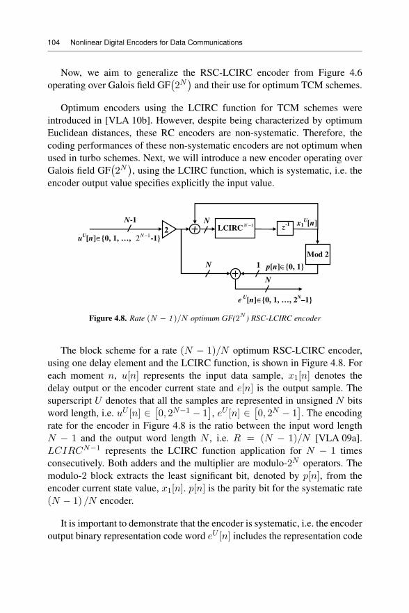
104 Nonlinear Digital Encoders for Data Communications
Now, we aim to generalize the RSC-LCIRC encoder from Figure 4.6operating over Galois field GF 2N and their use for optimum TCM schemes.
Optimum encoders using the LCIRC function for TCM schemes wereintroduced in [VLA 10b]. However, despite being characterized by optimumEuclidean distances, these RC encoders are non-systematic. Therefore, thecoding performances of these non-systematic encoders are not optimum whenused in turbo schemes. Next, we will introduce a new encoder operating overGalois field GF 2N , using the LCIRC function, which is systematic, i.e. theencoder output value specifies explicitly the input value.
uU[n]∈{0, 1, …,
12
−N-1}
eU[n]∈{0, 1, …, 2
N–1}
2 z-1 x1
U[n]1−N
LCIRCN-1
N
N
N
p[n]∈{0, 1}1
Mod 2
Figure 4.8. Rate (N − 1 )/N optimum GF(2N ) RSC-LCIRC encoder
The block scheme for a rate (N − 1)/N optimum RSC-LCIRC encoder,using one delay element and the LCIRC function, is shown in Figure 4.8. Foreach moment n, u[n] represents the input data sample, x1[n] denotes thedelay output or the encoder current state and e[n] is the output sample. Thesuperscript U denotes that all the samples are represented in unsigned N bitsword length, i.e. uU [n] ∈ 0, 2N−1 − 1 , eU [n] ∈ 0, 2N − 1 . The encodingrate for the encoder in Figure 4.8 is the ratio between the input word lengthN − 1 and the output word length N , i.e. R = (N − 1)/N [VLA 09a].LCIRCN−1 represents the LCIRC function application for N − 1 timesconsecutively. Both adders and the multiplier are modulo-2N operators. Themodulo-2 block extracts the least significant bit, denoted by p[n], from theencoder current state value, x1[n]. p[n] is the parity bit for the systematic rate(N − 1) /N encoder.
It is important to demonstrate that the encoder is systematic, i.e. the encoderoutput binary representation code word eU [n] includes the representation code
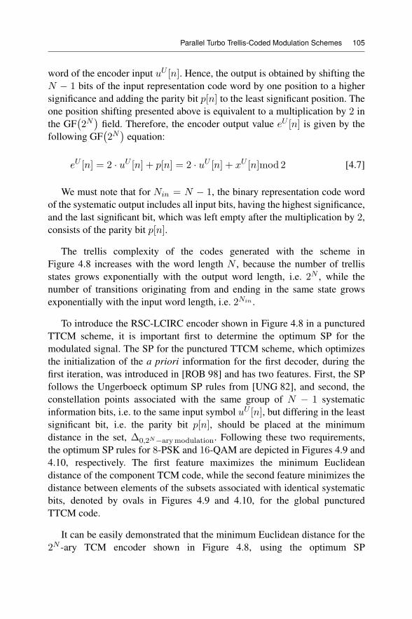
Parallel Turbo Trellis-Coded Modulation Schemes 105
word of the encoder input uU [n]. Hence, the output is obtained by shifting theN − 1 bits of the input representation code word by one position to a highersignificance and adding the parity bit p[n] to the least significant position. Theone position shifting presented above is equivalent to a multiplication by 2 inthe GF 2N field. Therefore, the encoder output value eU [n] is given by thefollowing GF 2N equation:
eU [n] = 2 · uU [n] + p[n] = 2 · uU [n] + xU [n]mod 2 [4.7]
We must note that for Nin = N − 1, the binary representation code wordof the systematic output includes all input bits, having the highest significance,and the last significant bit, which was left empty after the multiplication by 2,consists of the parity bit p[n].
The trellis complexity of the codes generated with the scheme inFigure 4.8 increases with the word length N , because the number of trellisstates grows exponentially with the output word length, i.e. 2N , while thenumber of transitions originating from and ending in the same state growsexponentially with the input word length, i.e. 2Nin .
To introduce the RSC-LCIRC encoder shown in Figure 4.8 in a puncturedTTCM scheme, it is important first to determine the optimum SP for themodulated signal. The SP for the punctured TTCM scheme, which optimizesthe initialization of the a priori information for the first decoder, during thefirst iteration, was introduced in [ROB 98] and has two features. First, the SPfollows the Ungerboeck optimum SP rules from [UNG 82], and second, theconstellation points associated with the same group of N − 1 systematicinformation bits, i.e. to the same input symbol uU [n], but differing in the leastsignificant bit, i.e. the parity bit p[n], should be placed at the minimumdistance in the set, Δ0,2N−arymodulation. Following these two requirements,the optimum SP rules for 8-PSK and 16-QAM are depicted in Figures 4.9 and4.10, respectively. The first feature maximizes the minimum Euclideandistance of the component TCM code, while the second feature minimizes thedistance between elements of the subsets associated with identical systematicbits, denoted by ovals in Figures 4.9 and 4.10, for the global puncturedTTCM code.
It can be easily demonstrated that the minimum Euclidean distance for the2N -ary TCM encoder shown in Figure 4.8, using the optimum SP
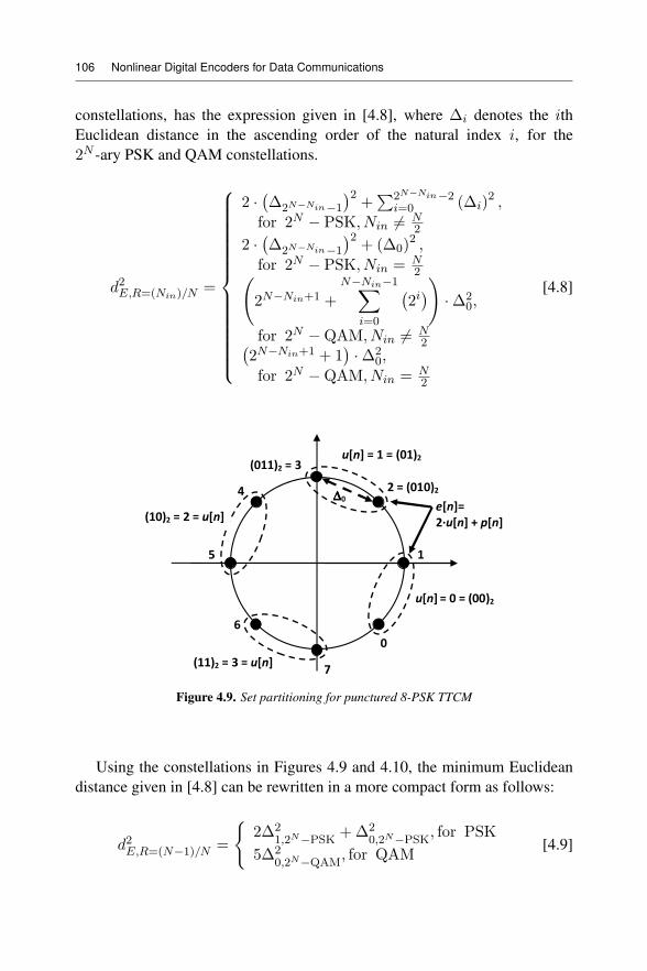
106 Nonlinear Digital Encoders for Data Communications
constellations, has the expression given in [4.8], where Δi denotes the ithEuclidean distance in the ascending order of the natural index i, for the2N -ary PSK and QAM constellations.
d2E,R=(Nin)/N=
⎧⎪⎪⎪⎪⎪⎪⎪⎪⎪⎪⎪⎪⎪⎪⎨⎪⎪⎪⎪⎪⎪⎪⎪⎪⎪⎪⎪⎪⎪⎩
2 · Δ2N−Nin−12+ 2N−Nin−2
i=0 (Δi)2 ,
for 2N − PSK, Nin = N2
2 · Δ2N−Nin−12+ (Δ0)
2 ,
for 2N − PSK, Nin = N2
2N−Nin+1 +
N−Nin−1
i=0
2i ·Δ20,
for 2N −QAM, Nin = N2
2N−Nin+1 + 1 ·Δ20,
for 2N −QAM, Nin = N2
[4.8]
ΔΔΔΔ
Figure 4.9. Set partitioning for punctured 8-PSK TTCM
Using the constellations in Figures 4.9 and 4.10, the minimum Euclideandistance given in [4.8] can be rewritten in a more compact form as follows:
d2E,R=(N−1)/N =2Δ2
1,2N−PSK+Δ2
0,2N−PSK, for PSK
5Δ20,2N−QAM
, for QAM[4.9]
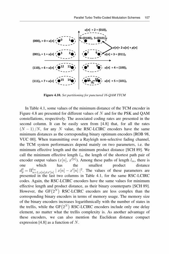
Parallel Turbo Trellis-Coded Modulation Schemes 107
ΔΔΔΔ
Figure 4.10. Set partitioning for punctured 16-QAM TTCM
In Table 4.1, some values of the minimum distance of the TCM encoder inFigure 4.8 are presented for different values of N and for the PSK and QAMconstellations, respectively. The associated coding rates are presented in thesecond column. It can be easily seen from [4.8] that, for all the rates(N − 1) /N , for any N value, the RSC-LCIRC encoders have the sameminimum distances as the corresponding binary optimum encoders [ROB 98,VUC 00]. When transmitting over a Rayleigh non-selective fading channel,the TCM system performances depend mainly on two parameters, i.e. theminimum effective length and the minimum product distance [SCH 89]. Wecall the minimum effective length lm the length of the shortest path pair ofencoder output values (x[n], x [n]). Among these paths of length lm, there isone which has the smallest product distanced2p = Πlm
n=1,x[n]=x [n] | x[n]− x [n] |2. The values of these parameters arepresented in the last two columns in Table 4.1, for the same RSC-LCIRCcodes. Again, the RSC-LCIRC encoders have the same values for minimumeffective length and product distance, as their binary counterparts [SCH 89].However, the GF 2N RSC-LCIRC encoders are less complex than thecorresponding binary encoders in terms of memory usage. The memory sizeof the binary encoders increases logarithmically with the number of states inthe trellis, while the GF 2N RSC-LCIRC encoders include only one delayelement, no matter what the trellis complexity is. As another advantage ofthese encoders, we can also mention the Euclidean distance compactexpression [4.8] as a function of N .
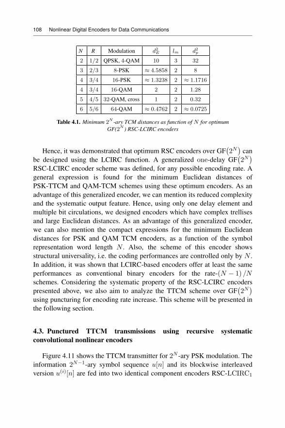
108 Nonlinear Digital Encoders for Data Communications
N R Modulation d2E lm d2p
2 1/2 QPSK, 4-QAM 10 3 32
3 2/3 8-PSK ≈ 4.5858 2 8
4 3/4 16-PSK ≈ 1.3238 2 ≈ 1.1716
4 3/4 16-QAM 2 2 1.28
5 4/5 32-QAM, cross 1 2 0.32
6 5/6 64-QAM ≈ 0.4762 2 ≈ 0.0725
Table 4.1. Minimum 2N -ary TCM distances as function of N for optimumGF(2N ) RSC-LCIRC encoders
Hence, it was demonstrated that optimum RSC encoders over GF 2N canbe designed using the LCIRC function. A generalized one-delay GF 2N
RSC-LCIRC encoder scheme was defined, for any possible encoding rate. Ageneral expression is found for the minimum Euclidean distances ofPSK-TTCM and QAM-TCM schemes using these optimum encoders. As anadvantage of this generalized encoder, we can mention its reduced complexityand the systematic output feature. Hence, using only one delay element andmultiple bit circulations, we designed encoders which have complex trellisesand large Euclidean distances. As an advantage of this generalized encoder,we can also mention the compact expressions for the minimum Euclideandistances for PSK and QAM TCM encoders, as a function of the symbolrepresentation word length N . Also, the scheme of this encoder showsstructural universality, i.e. the coding performances are controlled only by N .In addition, it was shown that LCIRC-based encoders offer at least the sameperformances as conventional binary encoders for the rate-(N − 1) /Nschemes. Considering the systematic property of the RSC-LCIRC encoderspresented above, we also aim to analyze the TTCM scheme over GF 2N
using puncturing for encoding rate increase. This scheme will be presented inthe following section.
4.3. Punctured TTCM transmissions using recursive systematicconvolutional nonlinear encoders
Figure 4.11 shows the TTCM transmitter for 2N -ary PSK modulation. Theinformation 2N−1-ary symbol sequence u[n] and its blockwise interleavedversion u(i)[n] are fed into two identical component encoders RSC-LCIRC1
Parallel Turbo Trellis-Coded Modulation Schemes 109
and RSC-LCIRC2 of rate (N − 1) /N . The encoders’ outputs are selectedalternatively and mapped into 2N -ary modulated symbol sequence x[n]. Theoutput of the bottom encoder is deinterleaved according to the inverseoperation of the interleaver. This ensures that at the input of the symbolselector, the N − 1 information bits from the 2N−1-ary input symbol, partlydefining the encoded 2N -ary symbols of both the upper and lower input, areidentical [ROB 98]. Therefore, if the selector is switched on a symbol base,the mapper output is a punctured version of the two encoded sequences andthe N − 1 information bits appear only once, mapped in a single transmittedsymbol selected either from e1[n] sequence or from e2[n] sequence.
e1[n]
e2(i)
[n]u(i)
[n]
u[n] RSC-
LCIRC1Signal
Mapper
RSC-
LCIRC2
Symbol
InterleaverSymbol
Deinterleaver
Symbol
Selector
e2[n]
Nin N
N
x[n]
Figure 4.11. TTCM transmitter with RSC-LCIRCencoders and symbol puncturing
Nevertheless, the remaining parity bit carried by the transmitted symbol istaken alternatively from the upper and lower encoders. Hence, the overallcoding rate for the scheme in Figure 4.11 is (N − 1) /N . The 2N -levelsmodulated symbol sequence is transmitted over a noisy and non-selectivefading channel. The received signal over the nth symbol interval is given by:
y[n] = h[n]x[n] + w[n] [4.10]
where w[n] is an AWGN sequence with E |w[n]|2 = N0 and x[n] denotesthe 2N -levels symbol value mapped from the encoders output sequences(e1[n], e2[n]) by puncturing over the nth symbol interval. The coefficient h[n]
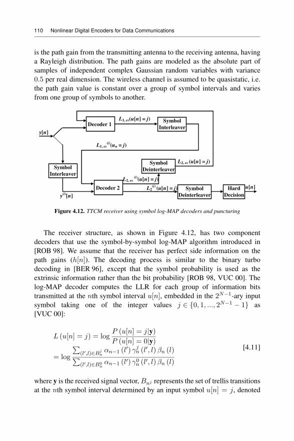
110 Nonlinear Digital Encoders for Data Communications
is the path gain from the transmitting antenna to the receiving antenna, havinga Rayleigh distribution. The path gains are modeled as the absolute part ofsamples of independent complex Gaussian random variables with variance0.5 per real dimension. The wireless channel is assumed to be quasistatic, i.e.the path gain value is constant over a group of symbol intervals and variesfrom one group of symbols to another.
y[n]
u[n]
y(i)
[n]
Symbol
Interleaver
Symbol
Deinterleaver
Decoder 2
Symbol
Interleaver
Symbol
Deinterleaver
Decoder 1
L1, es
(i)(un = j)
L1, es(u[n] = j)
L2, es (u[n] = j)
L2, es
(i)(u[n] = j)
L2(i)
(u[n] = j) Hard
Decision
Figure 4.12. TTCM receiver using symbol log-MAP decoders and puncturing
The receiver structure, as shown in Figure 4.12, has two componentdecoders that use the symbol-by-symbol log-MAP algorithm introduced in[ROB 98]. We assume that the receiver has perfect side information on thepath gains (h[n]). The decoding process is similar to the binary turbodecoding in [BER 96], except that the symbol probability is used as theextrinsic information rather than the bit probability [ROB 98, VUC 00]. Thelog-MAP decoder computes the LLR for each group of information bitstransmitted at the nth symbol interval u[n], embedded in the 2N−1-ary inputsymbol taking one of the integer values j ∈ {0, 1, ..., 2N−1 − 1} as[VUC 00]:
L (u[n] = j) = logP (u[n] = j|y)P (u[n] = 0|y)
= log(l ,l)∈Bj
nαn−1 (l ) γ
jn (l , l)βn (l)
(l ,l)∈B0nαn−1 (l ) γ0n (l , l)βn (l)
[4.11]
where y is the received signal vector, Bnj represents the set of trellis transitionsat the nth symbol interval determined by an input symbol u[n] = j, denoted
Parallel Turbo Trellis-Coded Modulation Schemes 111
as (Sn−1 = l → Sn = l) where Sn is the trellis state at moment n, and theprobabilities αn (l), βn (l) and γn (l , l), denoting the forward, backward andthe transition metrics, are computed recursively as in [VUC 00]. The symbol-by-symbol log-MAP decoder operates on an L symbols block basis. Hence, inall equations the symbol time variable n takes values between 1 and L. Thereceiver transition metric is given by:
γjn l , l =
⎧⎪⎨⎪⎩P (u[n]=j)P (u[n]=0) exp −|y[n]− x[n]|2
2σ2, if (l , l) ∈ Bj
n
0, otherwise
[4.12]
The transition metric in [4.12] is normalized over all input symbol valuesas follows:
γn l , l = log
2N−1−1
j=0
γjn l , l [4.13]
The first term in [4.12] denotes the a priori information for the transmittedinput symbol j. The number of trellis states for each component RSC-LCIRCencoder is 2N . The forward normalized metric is estimated as follows:
αn (l) = log
2N−1
l =0
exp αn−1 l + γn l , l [4.14]
The recurrence in [4.14] is initialized with:
α0(0) = 0; α0(l)|l=0 = −∞ [4.15]
The backward normalized metric is estimated as:
βn (l) = log2N−1
l =0
exp βn+1 l + γn+1 l , l [4.16]
112 Nonlinear Digital Encoders for Data Communications
and the recurrence in [4.16] is initialized with:
βL(0) = 0; βL(l)|l=0 = −∞ [4.17]
The input symbol j with the largest LLR in [4.11] is chosen as the harddecision output.
In contrast to the binary turbo codes, in the TTCM case, we cannotseparate the influence of the information and parity-check components withinone symbol. The systematic information and the extrinsic information are notindependent. Thus, both systematic and extrinsic information will beexchanged between the two component decoders. The joint extrinsic andsystematic information of the first log-MAP decoder, denoted asL1,es(u[n] = j), is computed as:
L1,es (u[n] = j) = L1 (u[n] = j)− logP (u[n] = j)
P (u[n] = 0)[4.18]
The last term in [4.18] represents the a priori information symbolknowledge fed by the other decoder.
The joint extrinsic and systematic information L1,es (u[n] = j) is used asthe estimate of the a priori LLR at the next decoding stage. After interleaving,this term is denoted as L
(i)1,es (u[n] = j). The joint extrinsic and systematic
information of the second decoder is given by:
L2,es(u[n] = j) = L2(u[n] = j)− L(i)1,es(u[n] = j) [4.19]
In the next iteration, the a priori term in [4.18] is replaced by thedeinterleaved joint extrinsic and systematic information from the seconddecoding stage, denoted as L(i)
2,es (u[n] = j).
It must be stated that for the symbol-by-symbol log-MAP decoding, eachcomponent decoder should avoid using the same systematic information twicein every iterative decoding step. In the TTCM scheme, each decoderalternately receives the noisy output of its own encoder and that of the otherencoder. As mentioned before, the parity bit in every second received symbol
Parallel Turbo Trellis-Coded Modulation Schemes 113
was generated by the other encoder, due to the symbol puncturing in thetransmitter. The decoder ignores this symbol by setting the branch metric tozero. The only input at this decoding step consists of the a priori componentobtained from the other decoder, which contains the systematic information.All the mentioned LLRs and the relations between them are represented in theTTCM receiver scheme in Figure 4.12.
The iterative metric computation presented above assumes that the a prioriLLR is already available. Nevertheless, in the first iteration, the a priori LLRfor the first decoder is unavailable. Considering the symbol mapping shown inFigure 4.9, the a priori information for the first decoder regarding thepunctured symbols, i.e. the input symbols encoded by the second encoder andtransmitted in the even positions n, is determined partially by the systematicinformation input symbol u[n] and also by the unknown parity bitp[n] ∈ {0, 1} generated by the second encoder (see equation [4.7]). Using themixed Bayes’ rule, the a priori probability is given by [ROB 98]:
P (u[n] = j) = const ·k∈{0,1}
p(y[n]|u[n] = j, p[n] = k) =
const ·k∈{0,1}
exp −|y[n]− h[n]xj, k[n]|22σ2
[4.20]
where const is a constant value, assuming that all the values of u[n] and p[n]are equally probable, and the 2N -ary modulated symbol x[n], transmitted bythe second encoder, is given by xj,k[n] = 2 · u[n] + p[n] = 2 · j + k. The apriori LLR is computed by normalizing the values in [4.20] by their sumestimated for all the values of j ∈ {0, 1, ..., 2N−1 − 1}. If the first decoderoperates over the odd symbols x[n], the a priori LLR is initialized withequally probable values assuming that Pr (u[n] = j) = 1/2N−1.
It was shown that the proposed optimum RSC-LCIRC encoder can be usedas a component encoder in TTCM schemes with punctured parity check bits(symbols). Also, due to the inner non-binary operation of the RSC-LCIRCencoder, the symbol-by-symbol log-MAP algorithm proves to be suitable foriterative decoding. The nonlinear LCIRC function leads to low complexityencoders, while the systematic property attains good performances inpunctured schemes.
114 Nonlinear Digital Encoders for Data Communications
4.4. Extrinsic information transfer (EXIT) charts analysis for TTCMschemes using nonlinear RSC encoders
A very important tool for the iterative decoding performances analysisconsists of the extrinsic information transfer (EXIT) chart, which describesthe extrinsic mutual information exchange between constituent decoders. Acomplexity efficient method for generating the symbol-based EXIT chartsfrom symbol-based a posteriori probabilities (APPs) was proposed in[KLI 06]. The expression for the average extrinsic information IE (u),estimated at the output of the decoder for the input symbol vector u, is givenby [KLI 06]:
IE,D (u) = N − 1
+1
L
L
n=1
E
⎡⎣2N−1
i=1
eD u(i)[n] · log2 eD u(i)[n]
⎤⎦ [4.21]
where L is the number of information symbols in the decoded block, N − 1is the number of information bits per input symbol, u(i)[n] is the presumedtransmitted information symbol at time instant n for i ∈ {1, 2, ..., 2N−1} ande (·) is the extrinsic probability. The expectation E [·] can be approximated bysimple time-averaging of the extrinsic probabilities of the information symbol.We propose to approximate the extrinsic probability as the normalized jointextrinsic and systematic information of the log-MAP decoder, from equations[4.18] and [4.19]:
eD u(i)[n] ≈ exp (LD,es (u[n] = i))2N−1
i=1 exp (LD,es (u[n] = i))[4.22]
In equations [4.21] and [4.22], D denotes the decoder number, i.e.D ∈ {1, 2}. However, computing an exact value of the extrinsic probabilityrequires that the systematic and parity parts of the channel observationvariables are independent. Thus, equation [4.22] represents only anapproximation of the true extrinsic information. The average a prioriinformation IA (u) is computed in a similar manner. The EXIT chart isobtained by representing, on the same diagram, the decoder 1 transfercharacteristic, i.e. IE,1 = T (IA,1) and the decoder 2 transfer characteristic,
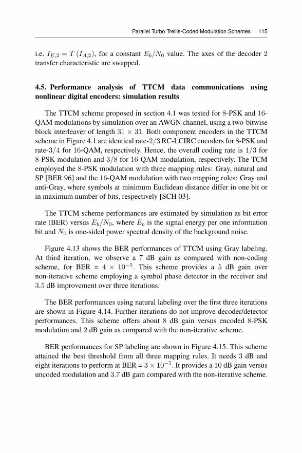
Parallel Turbo Trellis-Coded Modulation Schemes 115
i.e. IE,2 = T (IA,2), for a constant Eb/N0 value. The axes of the decoder 2transfer characteristic are swapped.
4.5. Performance analysis of TTCM data communications usingnonlinear digital encoders: simulation results
The TTCM scheme proposed in section 4.1 was tested for 8-PSK and 16-QAM modulations by simulation over an AWGN channel, using a two-bitwiseblock interleaver of length 31 × 31. Both component encoders in the TTCMscheme in Figure 4.1 are identical rate-2/3 RC-LCIRC encoders for 8-PSK andrate-3/4 for 16-QAM, respectively. Hence, the overall coding rate is 1/3 for8-PSK modulation and 3/8 for 16-QAM modulation, respectively. The TCMemployed the 8-PSK modulation with three mapping rules: Gray, natural andSP [BER 96] and the 16-QAM modulation with two mapping rules: Gray andanti-Gray, where symbols at minimum Euclidean distance differ in one bit orin maximum number of bits, respectively [SCH 03].
The TTCM scheme performances are estimated by simulation as bit errorrate (BER) versus Eb/N0, where Eb is the signal energy per one informationbit and N0 is one-sided power spectral density of the background noise.
Figure 4.13 shows the BER performances of TTCM using Gray labeling.At third iteration, we observe a 7 dB gain as compared with non-codingscheme, for BER = 4 × 10⁻⁵. This scheme provides a 5 dB gain overnon-iterative scheme employing a symbol phase detector in the receiver and3.5 dB improvement over three iterations.
The BER performances using natural labeling over the first three iterationsare shown in Figure 4.14. Further iterations do not improve decoder/detectorperformances. This scheme offers about 8 dB gain versus encoded 8-PSKmodulation and 2 dB gain as compared with the non-iterative scheme.
BER performances for SP labeling are shown in Figure 4.15. This schemeattained the best threshold from all three mapping rules. It needs 3 dB andeight iterations to perform at BER = 3× 10⁻⁵. It provides a 10 dB gain versusuncoded modulation and 3.7 dB gain compared with the non-iterative scheme.
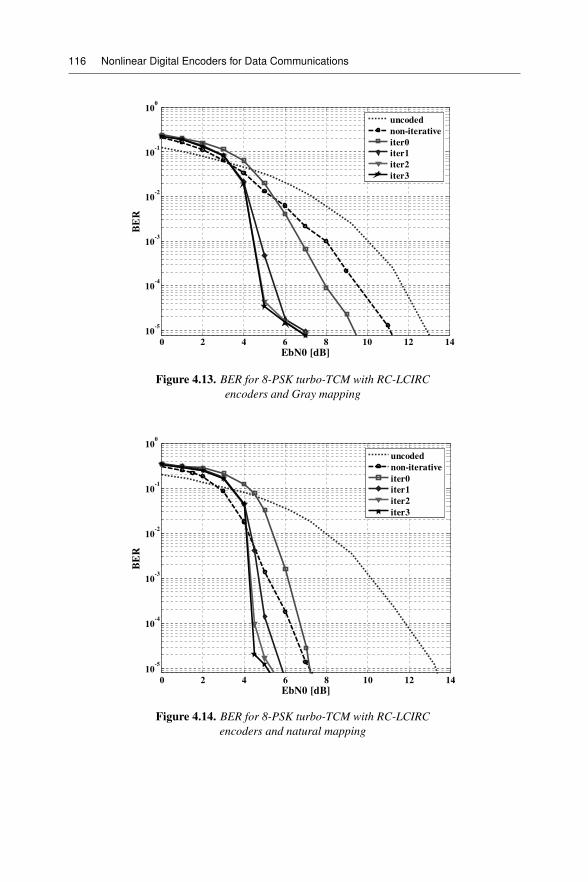
116 Nonlinear Digital Encoders for Data Communications
0 2 4 6 8 10 12 14
10-5
10-4
10-3
10-2
10-1
100
EbN0 [dB]
BE
R
uncoded
non-iterative
iter0
iter1
iter2
iter3
Figure 4.13. BER for 8-PSK turbo-TCM with RC-LCIRCencoders and Gray mapping
0 2 4 6 8 10 12 14
10-5
10-4
10-3
10-2
10-1
100
BE
R
EbN0 [dB]
uncoded
non-iterative
iter0
iter1
iter2
iter3
Figure 4.14. BER for 8-PSK turbo-TCM with RC-LCIRCencoders and natural mapping
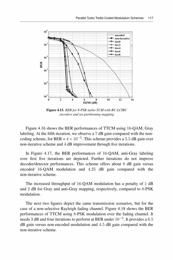
Parallel Turbo Trellis-Coded Modulation Schemes 117
0 2 4 6 8 10 12 14
10-5
10-4
10-3
10-2
10-1
100
EbN0 [dB]
BE
R
uncoded
non-iterative
iter0
iter2
iter4
iter6
iter8
Figure 4.15. BER for 8-PSK turbo-TCM with RC-LCIRCencoders and set partitioning mapping
Figure 4.16 shows the BER performances of TTCM using 16-QAM, Graylabeling. At the fifth iteration, we observe a 7 dB gain compared with the non-coding scheme, for BER = 4× 10⁻⁵. This scheme provides a 5.5 dB gain overnon-iterative scheme and 4 dB improvement through five iterations.
In Figure 4.17, the BER performances of 16-QAM, anti-Gray labelingover first five iterations are depicted. Further iterations do not improvedecoder/detector performances. This scheme offers about 8 dB gain versusencoded 16-QAM modulation and 4.25 dB gain compared with thenon-iterative scheme.
The increased throughput of 16-QAM modulation has a penalty of 1 dBand 2 dB for Gray and anti-Gray mapping, respectively, compared to 8-PSKmodulation.
The next two figures depict the same transmission scenarios, but for thecase of a non-selective Rayleigh fading channel. Figure 4.18 shows the BERperformances of TTCM using 8-PSK modulation over the fading channel. Itneeds 3 dB and four iterations to perform at BER under 10−5. It provides a 6.5dB gain versus non-encoded modulation and 4.5 dB gain compared with thenon-iterative scheme.
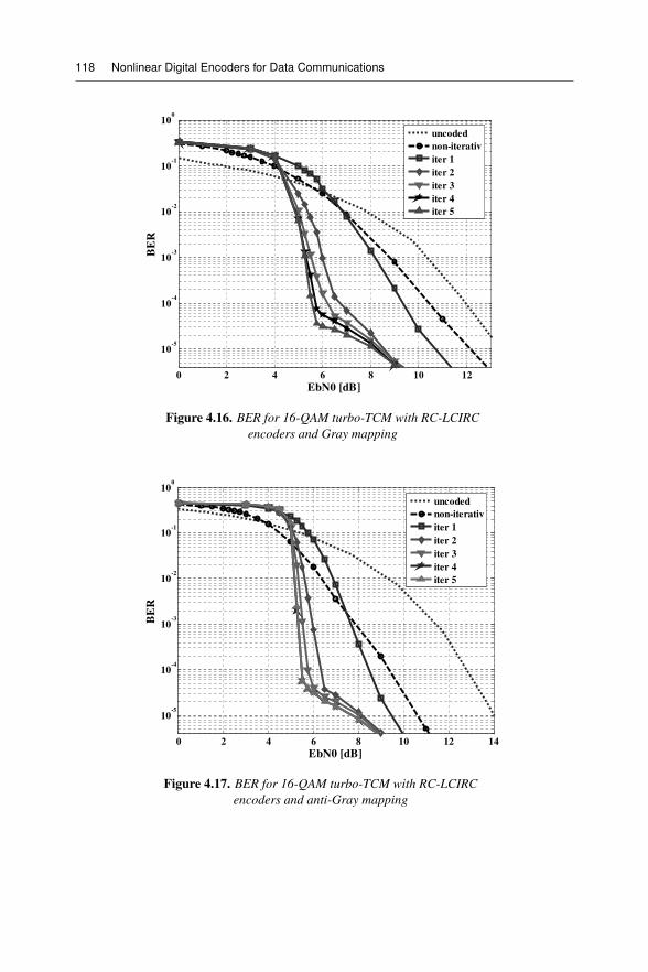
118 Nonlinear Digital Encoders for Data Communications
0 2 4 6 8 10 12
10-5
10-4
10-3
10-2
10-1
100
EbN0 [dB]
BE
R
uncoded
non-iterativ
iter 1
iter 2
iter 3
iter 4
iter 5
Figure 4.16. BER for 16-QAM turbo-TCM with RC-LCIRCencoders and Gray mapping
0 2 4 6 8 10 12 14
10-5
10-4
10-3
10-2
10-1
100
EbN0 [dB]
BE
R
uncoded
non-iterativ
iter 1
iter 2
iter 3
iter 4
iter 5
Figure 4.17. BER for 16-QAM turbo-TCM with RC-LCIRCencoders and anti-Gray mapping
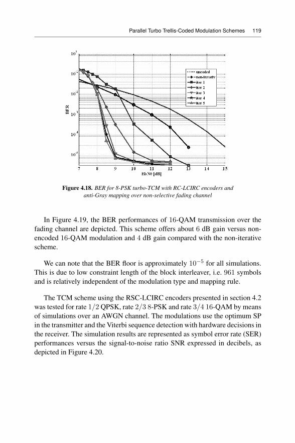
Parallel Turbo Trellis-Coded Modulation Schemes 119
Figure 4.18. BER for 8-PSK turbo-TCM with RC-LCIRC encoders andanti-Gray mapping over non-selective fading channel
In Figure 4.19, the BER performances of 16-QAM transmission over thefading channel are depicted. This scheme offers about 6 dB gain versus non-encoded 16-QAM modulation and 4 dB gain compared with the non-iterativescheme.
We can note that the BER floor is approximately 10−5 for all simulations.This is due to low constraint length of the block interleaver, i.e. 961 symbolsand is relatively independent of the modulation type and mapping rule.
The TCM scheme using the RSC-LCIRC encoders presented in section 4.2was tested for rate 1/2 QPSK, rate 2/3 8-PSK and rate 3/4 16-QAM by meansof simulations over an AWGN channel. The modulations use the optimum SPin the transmitter and the Viterbi sequence detection with hardware decisions inthe receiver. The simulation results are represented as symbol error rate (SER)performances versus the signal-to-noise ratio SNR expressed in decibels, asdepicted in Figure 4.20.
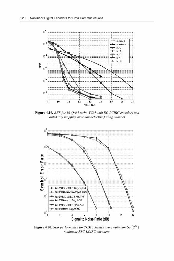
120 Nonlinear Digital Encoders for Data Communications
Figure 4.19. BER for 16-QAM turbo-TCM with RC-LCIRC encoders andanti-Gray mapping over non-selective fading channel
0 2 4 6 8 10 12 1410
-5
10-4
10-3
10-2
10-1
100
Signal to Noise Ratio (dB)
Sy
mb
ol
Err
or
Ra
te
Rate 3/4 RSC-LCIRC, 16-QAM, N=4
Rate 3/4 bin., [23,35,33,37]8, 16-QAM
Rate 2/3 RSC-LCIRC, 8-PSK, N=3
Rate 2/3 binary, [11,2,4]8, 8-PSK
Rate 1/2 RSC-LCIRC, QPSK, N=2
Rate 1/2 binary, [5,2]8, QPSK
Figure 4.20. SER performance for TCM schemes using optimum GF 2N
nonlinear RSC-LCIRC encoders
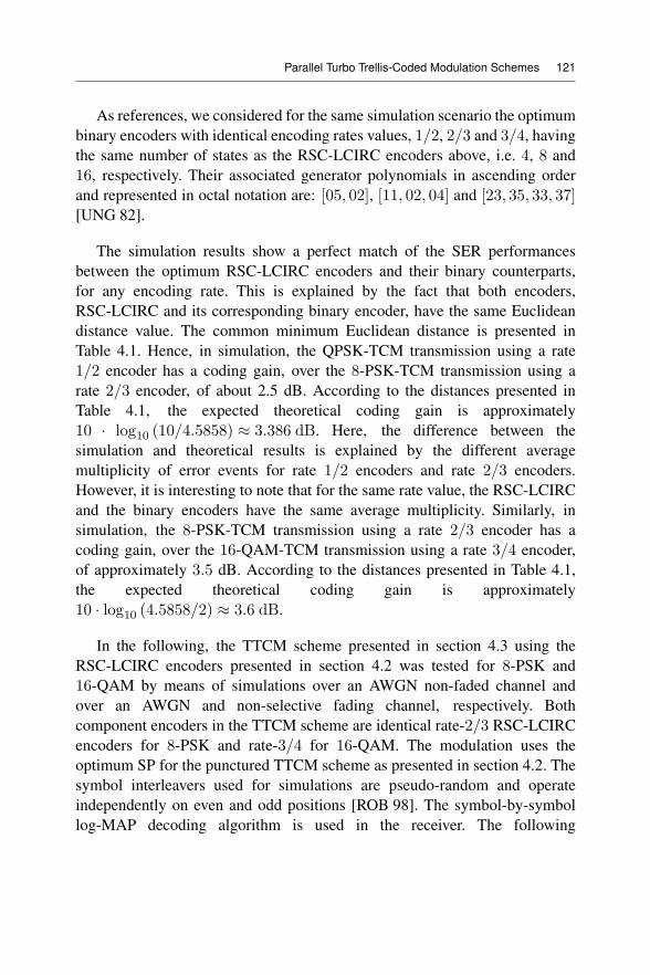
Parallel Turbo Trellis-Coded Modulation Schemes 121
As references, we considered for the same simulation scenario the optimumbinary encoders with identical encoding rates values, 1/2, 2/3 and 3/4, havingthe same number of states as the RSC-LCIRC encoders above, i.e. 4, 8 and16, respectively. Their associated generator polynomials in ascending orderand represented in octal notation are: [05, 02], [11, 02, 04] and [23, 35, 33, 37][UNG 82].
The simulation results show a perfect match of the SER performancesbetween the optimum RSC-LCIRC encoders and their binary counterparts,for any encoding rate. This is explained by the fact that both encoders,RSC-LCIRC and its corresponding binary encoder, have the same Euclideandistance value. The common minimum Euclidean distance is presented inTable 4.1. Hence, in simulation, the QPSK-TCM transmission using a rate1/2 encoder has a coding gain, over the 8-PSK-TCM transmission using arate 2/3 encoder, of about 2.5 dB. According to the distances presented inTable 4.1, the expected theoretical coding gain is approximately10 · log10 (10/4.5858) ≈ 3.386 dB. Here, the difference between thesimulation and theoretical results is explained by the different averagemultiplicity of error events for rate 1/2 encoders and rate 2/3 encoders.However, it is interesting to note that for the same rate value, the RSC-LCIRCand the binary encoders have the same average multiplicity. Similarly, insimulation, the 8-PSK-TCM transmission using a rate 2/3 encoder has acoding gain, over the 16-QAM-TCM transmission using a rate 3/4 encoder,of approximately 3.5 dB. According to the distances presented in Table 4.1,the expected theoretical coding gain is approximately10 · log10 (4.5858/2) ≈ 3.6 dB.
In the following, the TTCM scheme presented in section 4.3 using theRSC-LCIRC encoders presented in section 4.2 was tested for 8-PSK and16-QAM by means of simulations over an AWGN non-faded channel andover an AWGN and non-selective fading channel, respectively. Bothcomponent encoders in the TTCM scheme are identical rate-2/3 RSC-LCIRCencoders for 8-PSK and rate-3/4 for 16-QAM. The modulation uses theoptimum SP for the punctured TTCM scheme as presented in section 4.2. Thesymbol interleavers used for simulations are pseudo-random and operateindependently on even and odd positions [ROB 98]. The symbol-by-symbollog-MAP decoding algorithm is used in the receiver. The following
122 Nonlinear Digital Encoders for Data Communications
simulation results are represented as BER performances versus Eb/N0, whereEb is the signal energy per bit and N0 is the one-sided power spectral densityof the AWGN noise. The interleaver block includes 1, 024 symbols and thenumber of decoding iterations is eight. For all cases, further iterations do notsignificantly improve the BER performances. Figure 4.21 shows the BERperformances for TTCM transmission, using 8-PSK with bandwidthefficiency of 2 b/s/Hz, over the non-faded channel (i.e. hn = 1 in equation[4.10]). As a reference, we considered for the same simulation scenario thecorresponding rate-2/3 optimum binary encoder with eight states, determinedin [ROB 98] for 8-PSK TTCM with the generator polynomials, represented inoctal notation [11, 02, 04]. The simulation results show a perfect match of theBER performances between the rate-2/3 RSC-LCIRC encoder and its binarycounterpart. This is explained by the fact that both encoders have the sametrellis. The common minimum Euclidean distance is presented in Table 4.1.Eight iterations are enough to reach a BER of 3 × 10⁻⁵ forEb/N0 = 4.15 dB. In Figure 4.22, the BER performances of the 16-QAMtransmission over the non-fading channel, with bandwidth efficiency of 3b/s/Hz, are depicted. The rate-3/4 optimum binary encoder with 16 states,considered as reference, was determined in [VUC 00] for 16-QAM TTCMwith the generator polynomials [23, 35, 33, 37]. The results in Figure 4.22show two important features. First, the BER convergence for 16-QAM TTCMis faster than for 8-PSK case, and second, the RSC-LCIRC encoderoutperforms its binary counterpart at high Eb/N0 values. Hence, the binaryencoder gains less than 0.1 dB below an Eb/N0 = 5.8 dB threshold, whencompared to the corresponding RSC-LCIRC encoder. Above this threshold,the BER curves flatten and the RSC-LCIRC encoder outperforms its binarycounterpart by almost one order of BER. For both RSC-LCIRC and binaryencoders, eight iterations are enough to reach a BER of approximately1.7 × 10−5 for the threshold value of Eb/N0 = 5.8 dB. In Figure 4.23, BERperformances after eight iterations, for the same modulation schemestransmitting over the non-fading channel, are depicted when the interleaversize is varied. Therefore, the interleaver block consecutively includes 512,1, 024 and 2, 048 symbols. When the interleaver size is doubled, a codinggain of approximatively 0.4 dB is obtained for the 8-PSK modulation, whilefor 16-QAM modulation the coding gain varies between 0.2 and 0.5 dB.
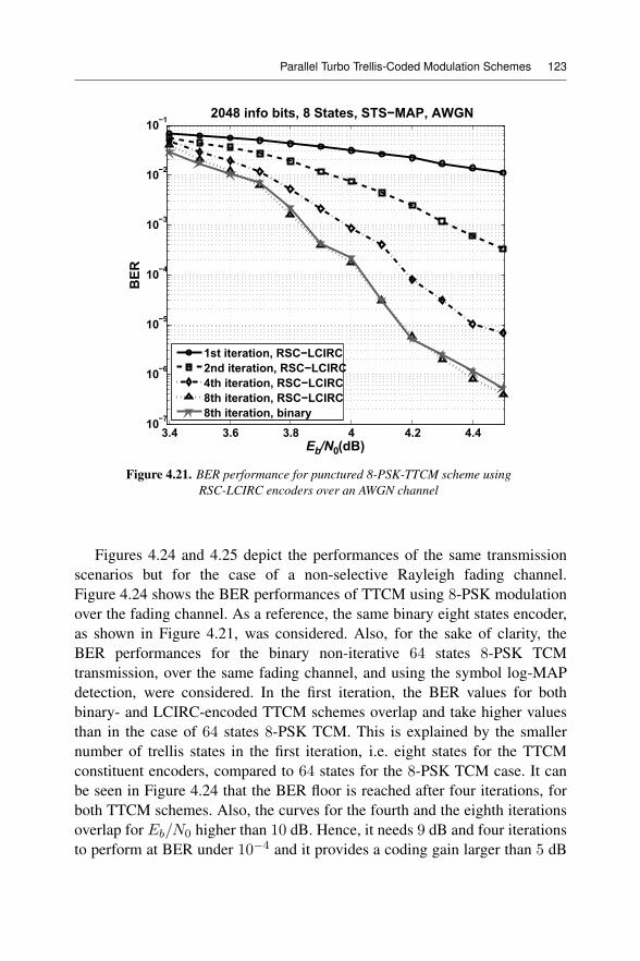
Parallel Turbo Trellis-Coded Modulation Schemes 123
Figure 4.21. BER performance for punctured 8-PSK-TTCM scheme usingRSC-LCIRC encoders over an AWGN channel
Figures 4.24 and 4.25 depict the performances of the same transmissionscenarios but for the case of a non-selective Rayleigh fading channel.Figure 4.24 shows the BER performances of TTCM using 8-PSK modulationover the fading channel. As a reference, the same binary eight states encoder,as shown in Figure 4.21, was considered. Also, for the sake of clarity, theBER performances for the binary non-iterative 64 states 8-PSK TCMtransmission, over the same fading channel, and using the symbol log-MAPdetection, were considered. In the first iteration, the BER values for bothbinary- and LCIRC-encoded TTCM schemes overlap and take higher valuesthan in the case of 64 states 8-PSK TCM. This is explained by the smallernumber of trellis states in the first iteration, i.e. eight states for the TTCMconstituent encoders, compared to 64 states for the 8-PSK TCM case. It canbe seen in Figure 4.24 that the BER floor is reached after four iterations, forboth TTCM schemes. Also, the curves for the fourth and the eighth iterationsoverlap for Eb/N0 higher than 10 dB. Hence, it needs 9 dB and four iterationsto perform at BER under 10−4 and it provides a coding gain larger than 5 dB
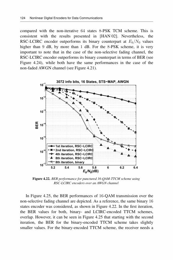
124 Nonlinear Digital Encoders for Data Communications
compared with the non-iterative 64 states 8-PSK TCM scheme. This isconsistent with the results presented in [HAN 02]. Nevertheless, theRSC-LCIRC encoder outperforms its binary counterpart at Eb/N0 valueshigher than 9 dB, by more than 1 dB. For the 8-PSK scheme, it is veryimportant to note that in the case of the non-selective fading channel, theRSC-LCIRC encoder outperforms its binary counterpart in terms of BER (seeFigure 4.24), while both have the same performances in the case of thenon-faded AWGN channel (see Figure 4.21).
Figure 4.22. BER performance for punctured 16-QAM-TTCM scheme usingRSC-LCIRC encoders over an AWGN channel
In Figure 4.25, the BER performances of 16-QAM transmission over thenon-selective fading channel are depicted. As a reference, the same binary 16states encoder was considered, as shown in Figure 4.22. In the first iteration,the BER values for both, binary- and LCIRC-encoded TTCM schemes,overlap. However, it can be seen in Figure 4.25 that starting with the seconditeration, the BER for the binary-encoded TTCM scheme takes slightlysmaller values. For the binary-encoded TTCM scheme, the receiver needs a
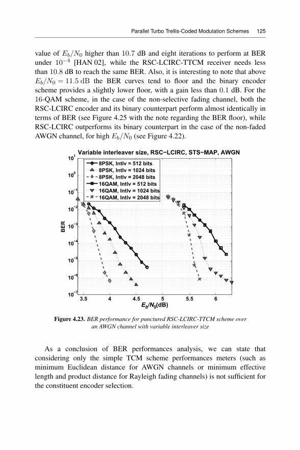
Parallel Turbo Trellis-Coded Modulation Schemes 125
value of Eb/N0 higher than 10.7 dB and eight iterations to perform at BERunder 10−4 [HAN 02], while the RSC-LCIRC-TTCM receiver needs lessthan 10.8 dB to reach the same BER. Also, it is interesting to note that aboveEb/N0 = 11.5 dB the BER curves tend to floor and the binary encoderscheme provides a slightly lower floor, with a gain less than 0.1 dB. For the16-QAM scheme, in the case of the non-selective fading channel, both theRSC-LCIRC encoder and its binary counterpart perform almost identically interms of BER (see Figure 4.25 with the note regarding the BER floor), whileRSC-LCIRC outperforms its binary counterpart in the case of the non-fadedAWGN channel, for high Eb/N0 (see Figure 4.22).
Figure 4.23. BER performance for punctured RSC-LCIRC-TTCM scheme overan AWGN channel with variable interleaver size
As a conclusion of BER performances analysis, we can state thatconsidering only the simple TCM scheme performances meters (such asminimum Euclidean distance for AWGN channels or minimum effectivelength and product distance for Rayleigh fading channels) is not sufficient forthe constituent encoder selection.
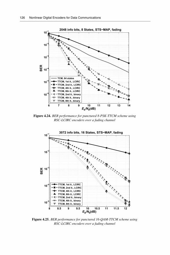
126 Nonlinear Digital Encoders for Data Communications
Figure 4.24. BER performance for punctured 8-PSK-TTCM scheme usingRSC-LCIRC encoders over a fading channel
Figure 4.25. BER performance for punctured 16-QAM-TTCM scheme usingRSC-LCIRC encoders over a fading channel
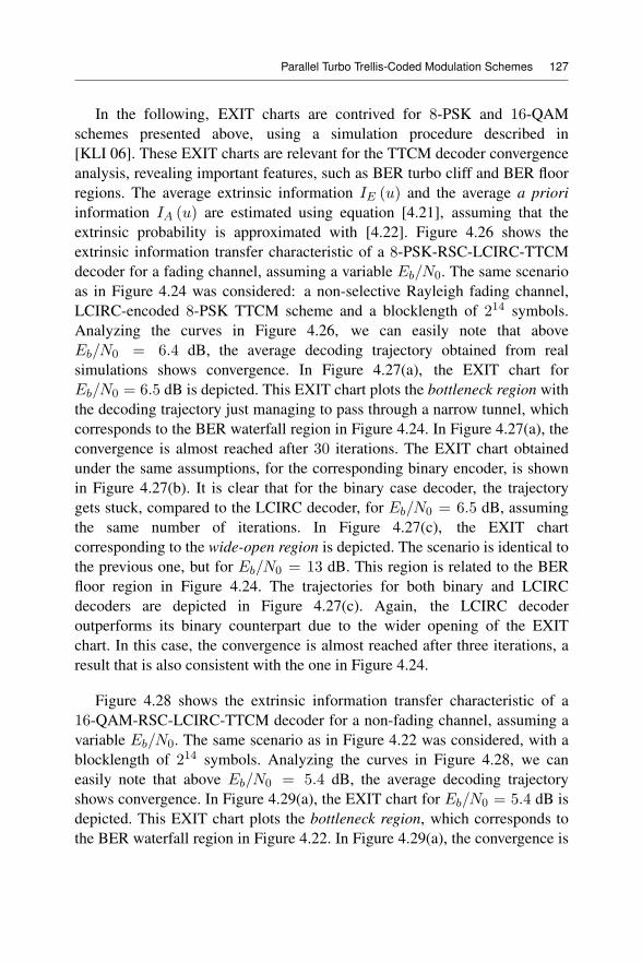
Parallel Turbo Trellis-Coded Modulation Schemes 127
In the following, EXIT charts are contrived for 8-PSK and 16-QAMschemes presented above, using a simulation procedure described in[KLI 06]. These EXIT charts are relevant for the TTCM decoder convergenceanalysis, revealing important features, such as BER turbo cliff and BER floorregions. The average extrinsic information IE (u) and the average a prioriinformation IA (u) are estimated using equation [4.21], assuming that theextrinsic probability is approximated with [4.22]. Figure 4.26 shows theextrinsic information transfer characteristic of a 8-PSK-RSC-LCIRC-TTCMdecoder for a fading channel, assuming a variable Eb/N0. The same scenarioas in Figure 4.24 was considered: a non-selective Rayleigh fading channel,LCIRC-encoded 8-PSK TTCM scheme and a blocklength of 214 symbols.Analyzing the curves in Figure 4.26, we can easily note that aboveEb/N0 = 6.4 dB, the average decoding trajectory obtained from realsimulations shows convergence. In Figure 4.27(a), the EXIT chart forEb/N0 = 6.5 dB is depicted. This EXIT chart plots the bottleneck region withthe decoding trajectory just managing to pass through a narrow tunnel, whichcorresponds to the BER waterfall region in Figure 4.24. In Figure 4.27(a), theconvergence is almost reached after 30 iterations. The EXIT chart obtainedunder the same assumptions, for the corresponding binary encoder, is shownin Figure 4.27(b). It is clear that for the binary case decoder, the trajectorygets stuck, compared to the LCIRC decoder, for Eb/N0 = 6.5 dB, assumingthe same number of iterations. In Figure 4.27(c), the EXIT chartcorresponding to the wide-open region is depicted. The scenario is identical tothe previous one, but for Eb/N0 = 13 dB. This region is related to the BERfloor region in Figure 4.24. The trajectories for both binary and LCIRCdecoders are depicted in Figure 4.27(c). Again, the LCIRC decoderoutperforms its binary counterpart due to the wider opening of the EXITchart. In this case, the convergence is almost reached after three iterations, aresult that is also consistent with the one in Figure 4.24.
Figure 4.28 shows the extrinsic information transfer characteristic of a16-QAM-RSC-LCIRC-TTCM decoder for a non-fading channel, assuming avariable Eb/N0. The same scenario as in Figure 4.22 was considered, with ablocklength of 214 symbols. Analyzing the curves in Figure 4.28, we caneasily note that above Eb/N0 = 5.4 dB, the average decoding trajectoryshows convergence. In Figure 4.29(a), the EXIT chart for Eb/N0 = 5.4 dB isdepicted. This EXIT chart plots the bottleneck region, which corresponds tothe BER waterfall region in Figure 4.22. In Figure 4.29(a), the convergence is
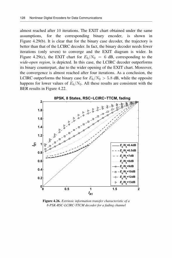
128 Nonlinear Digital Encoders for Data Communications
almost reached after 10 iterations. The EXIT chart obtained under the sameassumptions, for the corresponding binary encoder, is shown inFigure 4.29(b). It is clear that for the binary case decoder, the trajectory isbetter than that of the LCIRC decoder. In fact, the binary decoder needs feweriterations (only seven) to converge and the EXIT diagram is wider. InFigure 4.29(c), the EXIT chart for Eb/N0 = 6 dB, corresponding to thewide-open region, is depicted. In this case, the LCIRC decoder outperformsits binary counterpart, due to the wider opening of the EXIT chart. Moreover,the convergence is almost reached after four iterations. As a conclusion, theLCIRC outperforms the binary case for Eb/N0 > 5.8 dB, while the oppositehappens for lower values of Eb/N0. All these results are consistent with theBER results in Figure 4.22.
Figure 4.26. Extrinsic information transfer characteristic of a8-PSK-RSC-LCIRC-TTCM decoder for a fading channel
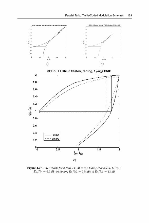
Parallel Turbo Trellis-Coded Modulation Schemes 129
a) b)
c)
Figure 4.27. EXIT charts for 8-PSK-TTCM over a fading channel. a) LCIRC,Eb/N0 = 6.5 dB; b) binary, Eb/N0 = 6.5 dB; c) Eb/N0 = 13 dB
130 Nonlinear Digital Encoders for Data Communications
Figure 4.28. Extrinsic information transfer characteristic of a16-QAM-RSC-LCIRC-TTCM decoder for a non-fading channel
For all EXIT charts mentioned above, a high initial value of the a prioriinformation is noted for the first decoder. This is explained by the goodapproximation provided by equation [4.20], in the first iteration initialization.
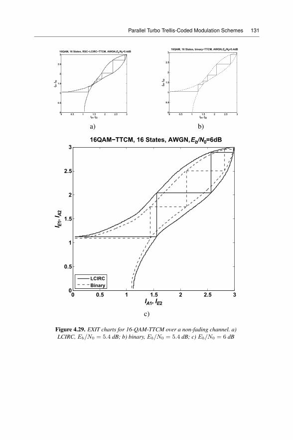
Parallel Turbo Trellis-Coded Modulation Schemes 131
a) b)
c)
Figure 4.29. EXIT charts for 16-QAM-TTCM over a non-fading channel. a)LCIRC, Eb/N0 = 5.4 dB; b) binary, Eb/N0 = 5.4 dB; c) Eb/N0 = 6 dB

Appendix
Demonstrations for the Properties of theUnsigned and Signed Finite Precision
Operators
A1.1. The demonstration of theorem 2.2
In section 2.2, the theorem 2.2 was enunciated with [2.19]. Therefore, theaddition operation in the 2N -set is associative, as expressed by:
wU = xU ⊕ yU ⊕ zU = xU ⊕ yU ⊕ zU = xU ⊕ yU ⊕ zU =
= xU + yU + zU mod 2N
wU ∈ 0, 2N − 1
[A1.1]
DEMONSTRATION A1.1.– According to definition 2.6 given in section 2.2,the addition operation for two unsigned numbers, in the 2N -set, is given byequation [2.13]:
vU = xU ⊕ yU =xU + yU − 2N if 2N ≤ xU + yU ≤ 2N+1 − 2
xU + yU if 0 ≤ xU + yU ≤ 2N − 1
vU ∈ 0, 2N − 1
[A1.2]
134 Nonlinear Digital Encoders for Data Communications
Let us consider the first term in [A1.1], w1U = xU ⊕ yU ⊕zU = vU⊕zU ,
and using equation [A1.2], it results in the following expression:
w1U = vU ⊕ zU = zU + vU mod 2N
=
⎧⎨⎩ zU + vU − 2N if 2N ≤ zU + vU ≤ 2N+1 − 2
zU + vU if 0 ≤ zU + vU ≤ 2N − 1
=
⎧⎪⎪⎪⎪⎪⎪⎪⎪⎪⎪⎪⎪⎪⎪⎪⎪⎪⎪⎪⎪⎪⎪⎪⎪⎪⎪⎪⎪⎪⎪⎪⎪⎪⎪⎪⎪⎪⎪⎪⎪⎨⎪⎪⎪⎪⎪⎪⎪⎪⎪⎪⎪⎪⎪⎪⎪⎪⎪⎪⎪⎪⎪⎪⎪⎪⎪⎪⎪⎪⎪⎪⎪⎪⎪⎪⎪⎪⎪⎪⎪⎪⎩
(xU+ yU − 2N ) + zU − 2N if 2N ≤ xU + yU − 2N + zU ≤≤ 2N+1 − 2 ∩∩ 2N ≤ xU + yU ≤ 2N+1 − 2 ∪∪ 0 ≤ zU ≤ 2N − 1
(xU+ yU − 2N ) + zU if 0 ≤ xU + yU − 2N + zU ≤≤ 2N − 1 ∩∩ 2N ≤ xU + yU ≤ 2N+1 − 2 ∪∪ 0 ≤ zU ≤ 2N − 1
(xU+ yU ) + zU − 2N if 2N ≤ xU + yU + zU ≤ 2N+1 − 2 ∩∩ 0 ≤ xU + yU ≤ 2N − 1 ∪∪ 0 ≤ zU ≤ 2N − 1
(xU+ yU ) + zU if 0 ≤ xU + yU + zU ≤ 2N − 1 ∩∩ 0 ≤ xU + yU ≤ 2N − 1 ∪∪ 0 ≤ zU ≤ 2N − 1
[A1.3]
Appendix 135
which is equivalent to:
w1U =
⎧⎪⎪⎪⎪⎪⎪⎪⎪⎪⎪⎪⎪⎪⎪⎪⎪⎪⎪⎪⎪⎪⎪⎪⎪⎪⎪⎪⎪⎪⎪⎪⎪⎪⎪⎪⎪⎪⎪⎪⎪⎪⎪⎨⎪⎪⎪⎪⎪⎪⎪⎪⎪⎪⎪⎪⎪⎪⎪⎪⎪⎪⎪⎪⎪⎪⎪⎪⎪⎪⎪⎪⎪⎪⎪⎪⎪⎪⎪⎪⎪⎪⎪⎪⎪⎪⎩
xU+ yU + zU if 0 ≤ xU + yU + zU ≤ 2N − 1 ∩∩ 0 ≤ xU + yU + zU ≤ 2N+1 − 2 =
= 0 ≤ xU + yU + zU ≤ 2N − 1
xU+ yU + zU − 2N if 2N ≤ xU + yU + zU ≤≤ 2N+1 − 2 ∩∩ 0 ≤ xU + yU + zU ≤ 2N+1 − 2 ∪ =
∪ 0 ≤ xU + yU + zU − 2N ≤ 2N − 1 ∩∩ 2N ≤ xU + yU + zU ≤ 2N · 3− 3 =
= 2N ≤ xU + yU + zU ≤ 2N+1 − 2 ∪∪ 2N ≤ xU + yU + zU ≤ 2N+1 − 1 =
= 2N ≤ xU + yU + zU ≤ 2N+1 − 1
xU+ yU + zU − 2N · 2 if 2N ≤ xU + yU + zU − 2N ≤≤ 2N+1 − 2 ∩∩ 2N ≤ xU + yU + zU ≤ 2N+1 + 2N − 1− 2 =
= 2N · 3− 3 =
= 2N+1 ≤ xU + yU + zU ≤ 2N · 3− 2 ∩∩ 2N ≤ xU + yU + zU ≤ 2N · 3− 3 =
= 2N+1 ≤ xU + yU + zU ≤ 2N · 3− 3
[A1.4]
So, we have:
w1U =
⎧⎪⎪⎪⎪⎪⎪⎪⎪⎪⎪⎨⎪⎪⎪⎪⎪⎪⎪⎪⎪⎪⎩
xU+ yU + zU
if 0 ≤ xU + yU + zU ≤ 2N − 1
xU+ yU + zU − 2N
if 2N ≤ xU + yU + zU ≤ 2N+1 − 1
xU+ yU + zU − 2 · 2Nif 2 · 2N ≤ xU + yU + zU ≤ 2N · 3− 3
[A1.5]
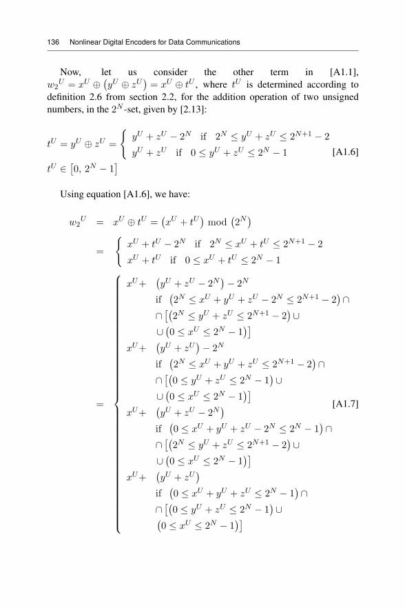
136 Nonlinear Digital Encoders for Data Communications
Now, let us consider the other term in [A1.1],w2
U = xU ⊕ yU ⊕ zU = xU ⊕ tU , where tU is determined according todefinition 2.6 from section 2.2, for the addition operation of two unsignednumbers, in the 2N -set, given by [2.13]:
tU = yU ⊕ zU =yU + zU − 2N if 2N ≤ yU + zU ≤ 2N+1 − 2
yU + zU if 0 ≤ yU + zU ≤ 2N − 1
tU ∈ 0, 2N − 1
[A1.6]
Using equation [A1.6], we have:
w2U = xU ⊕ tU = xU + tU mod 2N
=xU + tU − 2N if 2N ≤ xU + tU ≤ 2N+1 − 2
xU + tU if 0 ≤ xU + tU ≤ 2N − 1
=
⎧⎪⎪⎪⎪⎪⎪⎪⎪⎪⎪⎪⎪⎪⎪⎪⎪⎪⎪⎪⎪⎪⎪⎪⎪⎪⎪⎪⎪⎪⎪⎪⎪⎪⎪⎪⎪⎪⎨⎪⎪⎪⎪⎪⎪⎪⎪⎪⎪⎪⎪⎪⎪⎪⎪⎪⎪⎪⎪⎪⎪⎪⎪⎪⎪⎪⎪⎪⎪⎪⎪⎪⎪⎪⎪⎪⎩
xU+ yU + zU − 2N − 2N
if 2N ≤ xU + yU + zU − 2N ≤ 2N+1 − 2 ∩∩ 2N ≤ yU + zU ≤ 2N+1 − 2 ∪∪ 0 ≤ xU ≤ 2N − 1
xU+ yU + zU − 2N
if 2N ≤ xU + yU + zU ≤ 2N+1 − 2 ∩∩ 0 ≤ yU + zU ≤ 2N − 1 ∪∪ 0 ≤ xU ≤ 2N − 1
xU+ yU + zU − 2N
if 0 ≤ xU + yU + zU − 2N ≤ 2N − 1 ∩∩ 2N ≤ yU + zU ≤ 2N+1 − 2 ∪∪ 0 ≤ xU ≤ 2N − 1
xU+ yU + zU
if 0 ≤ xU + yU + zU ≤ 2N − 1 ∩∩ 0 ≤ yU + zU ≤ 2N − 1 ∪0 ≤ xU ≤ 2N − 1
[A1.7]
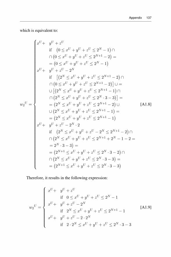
Appendix 137
which is equivalent to:
w2U =
⎧⎪⎪⎪⎪⎪⎪⎪⎪⎪⎪⎪⎪⎪⎪⎪⎪⎪⎪⎪⎪⎪⎪⎪⎪⎪⎪⎪⎪⎪⎪⎪⎪⎪⎪⎪⎪⎪⎪⎪⎪⎪⎪⎪⎪⎪⎨⎪⎪⎪⎪⎪⎪⎪⎪⎪⎪⎪⎪⎪⎪⎪⎪⎪⎪⎪⎪⎪⎪⎪⎪⎪⎪⎪⎪⎪⎪⎪⎪⎪⎪⎪⎪⎪⎪⎪⎪⎪⎪⎪⎪⎪⎩
xU+ yU + zU
if 0 ≤ xU + yU + zU ≤ 2N − 1 ∩∩ 0 ≤ xU + yU + zU ≤ 2N+1 − 2 =
= 0 ≤ xU + yU + zU ≤ 2N − 1
xU+ yU + zU − 2N
if 2N ≤ xU + yU + zU ≤ 2N+1 − 2 ∩∩ 0 ≤ xU + yU + zU ≤ 2N+1 − 2 ∪ =
∪ 2N ≤ xU + yU + zU ≤ 2N+1 − 1 ∩∩ 2N ≤ xU + yU + zU ≤ 2N · 3− 3 =
= 2N ≤ xU + yU + zU ≤ 2N+1 − 2 ∪∪ 2N ≤ xU + yU + zU ≤ 2N+1 − 1 =
= 2N ≤ xU + yU + zU ≤ 2N+1 − 1
xU+ yU + zU − 2N · 2if 2N ≤ xU + yU + zU − 2N ≤ 2N+1 − 2 ∩∩ 2N ≤ xU + yU + zU ≤ 2N+1 + 2N − 1− 2 =
= 2N · 3− 3 =
= 2N+1 ≤ xU + yU + zU ≤ 2N · 3− 2 ∩∩ 2N ≤ xU + yU + zU ≤ 2N · 3− 3 =
= 2N+1 ≤ xU + yU + zU ≤ 2N · 3− 3
[A1.8]
Therefore, it results in the following expression:
w2U =
⎧⎪⎪⎪⎪⎪⎪⎪⎪⎪⎪⎨⎪⎪⎪⎪⎪⎪⎪⎪⎪⎪⎩
xU+ yU + zU
if 0 ≤ xU + yU + zU ≤ 2N − 1
xU+ yU + zU − 2N
if 2N ≤ xU + yU + zU ≤ 2N+1 − 1
xU+ yU + zU − 2 · 2Nif 2 · 2N ≤ xU + yU + zU ≤ 2N · 3− 3
[A1.9]
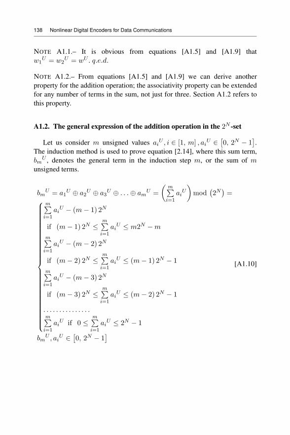
138 Nonlinear Digital Encoders for Data Communications
NOTE A1.1.– It is obvious from equations [A1.5] and [A1.9] thatw1
U = w2U = wU . q.e.d.
NOTE A1.2.– From equations [A1.5] and [A1.9] we can derive anotherproperty for the addition operation; the associativity property can be extendedfor any number of terms in the sum, not just for three. Section A1.2 refers tothis property.
A1.2. The general expression of the addition operation in the 2N -set
Let us consider m unsigned values aiU , i ∈ [1, m] , ai
U ∈ 0, 2N − 1 .The induction method is used to prove equation [2.14], where this sum term,bm
U , denotes the general term in the induction step m, or the sum of munsigned terms.
bmU = a1
U ⊕ a2U ⊕ a3
U ⊕ . . .⊕ amU =
m
i=1ai
U mod 2N =⎧⎪⎪⎪⎪⎪⎪⎪⎪⎪⎪⎪⎪⎪⎪⎪⎪⎪⎪⎪⎪⎪⎪⎪⎪⎨⎪⎪⎪⎪⎪⎪⎪⎪⎪⎪⎪⎪⎪⎪⎪⎪⎪⎪⎪⎪⎪⎪⎪⎪⎩
m
i=1ai
U − (m− 1) 2N
if (m− 1) 2N ≤m
i=1ai
U ≤ m2N −m
m
i=1ai
U − (m− 2) 2N
if (m− 2) 2N ≤m
i=1ai
U ≤ (m− 1) 2N − 1
m
i=1ai
U − (m− 3) 2N
if (m− 3) 2N ≤m
i=1ai
U ≤ (m− 2) 2N − 1
. . . . . . . . . . . . . . .m
i=1ai
U if 0 ≤m
i=1ai
U ≤ 2N − 1
bmU , ai
U ∈ 0, 2N − 1
[A1.10]
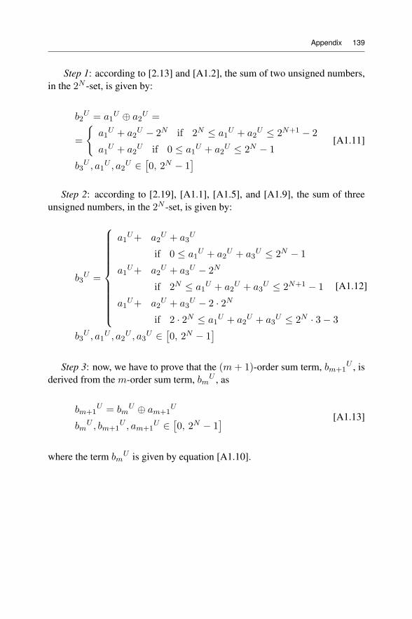
Appendix 139
Step 1: according to [2.13] and [A1.2], the sum of two unsigned numbers,in the 2N -set, is given by:
b2U = a1
U ⊕ a2U =
=a1
U + a2U − 2N if 2N ≤ a1
U + a2U ≤ 2N+1 − 2
a1U + a2
U if 0 ≤ a1U + a2
U ≤ 2N − 1
b3U , a1
U , a2U ∈ 0, 2N − 1
[A1.11]
Step 2: according to [2.19], [A1.1], [A1.5], and [A1.9], the sum of threeunsigned numbers, in the 2N -set, is given by:
b3U =
⎧⎪⎪⎪⎪⎪⎪⎪⎪⎪⎪⎨⎪⎪⎪⎪⎪⎪⎪⎪⎪⎪⎩
a1U+ a2
U + a3U
if 0 ≤ a1U + a2
U + a3U ≤ 2N − 1
a1U+ a2
U + a3U − 2N
if 2N ≤ a1U + a2
U + a3U ≤ 2N+1 − 1
a1U+ a2
U + a3U − 2 · 2N
if 2 · 2N ≤ a1U + a2
U + a3U ≤ 2N · 3− 3
b3U , a1
U , a2U , a3
U ∈ 0, 2N − 1
[A1.12]
Step 3: now, we have to prove that the (m+ 1)-order sum term, bm+1U , is
derived from the m-order sum term, bmU , as
bm+1U = bm
U ⊕ am+1U
bmU , bm+1
U , am+1U ∈ 0, 2N − 1
[A1.13]
where the term bmU is given by equation [A1.10].
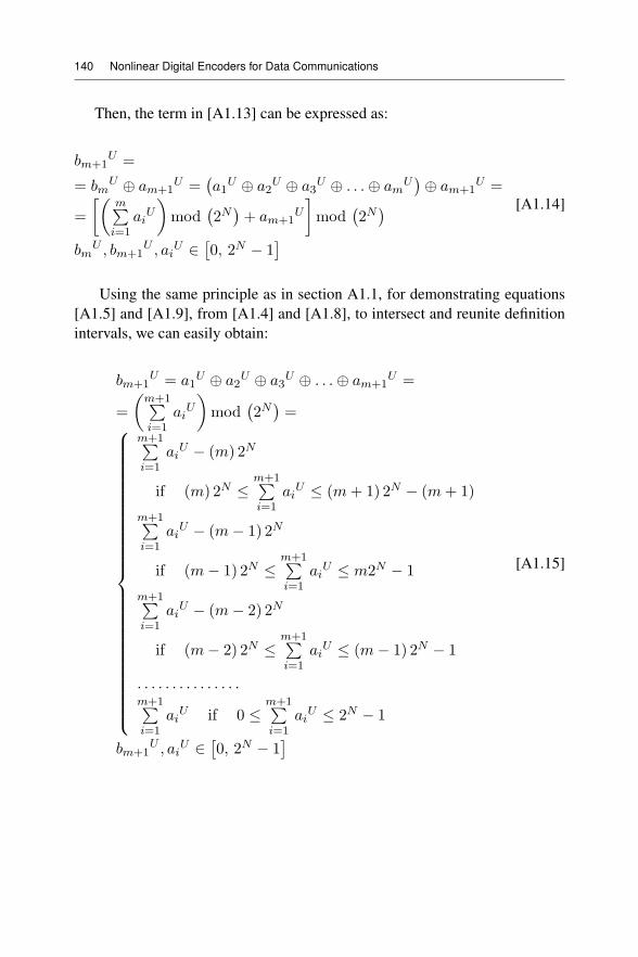
140 Nonlinear Digital Encoders for Data Communications
Then, the term in [A1.13] can be expressed as:
bm+1U =
= bmU ⊕ am+1
U = a1U ⊕ a2
U ⊕ a3U ⊕ . . .⊕ am
U ⊕ am+1U =
=m
i=1ai
U mod 2N + am+1U mod 2N
bmU , bm+1
U , aiU ∈ 0, 2N − 1
[A1.14]
Using the same principle as in section A1.1, for demonstrating equations[A1.5] and [A1.9], from [A1.4] and [A1.8], to intersect and reunite definitionintervals, we can easily obtain:
bm+1U = a1
U ⊕ a2U ⊕ a3
U ⊕ . . .⊕ am+1U =
=m+1
i=1ai
U mod 2N =⎧⎪⎪⎪⎪⎪⎪⎪⎪⎪⎪⎪⎪⎪⎪⎪⎪⎪⎪⎪⎪⎪⎪⎪⎪⎪⎪⎨⎪⎪⎪⎪⎪⎪⎪⎪⎪⎪⎪⎪⎪⎪⎪⎪⎪⎪⎪⎪⎪⎪⎪⎪⎪⎪⎩
m+1
i=1ai
U − (m) 2N
if (m) 2N ≤m+1
i=1ai
U ≤ (m+ 1) 2N − (m+ 1)
m+1
i=1ai
U − (m− 1) 2N
if (m− 1) 2N ≤m+1
i=1ai
U ≤ m2N − 1
m+1
i=1ai
U − (m− 2) 2N
if (m− 2) 2N ≤m+1
i=1ai
U ≤ (m− 1) 2N − 1
. . . . . . . . . . . . . . .m+1
i=1ai
U if 0 ≤m+1
i=1ai
U ≤ 2N − 1
bm+1U , ai
U ∈ 0, 2N − 1
[A1.15]
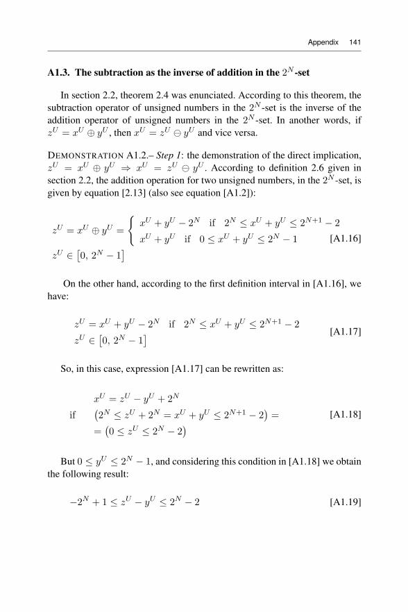
Appendix 141
A1.3. The subtraction as the inverse of addition in the 2N -set
In section 2.2, theorem 2.4 was enunciated. According to this theorem, thesubtraction operator of unsigned numbers in the 2N -set is the inverse of theaddition operator of unsigned numbers in the 2N -set. In another words, ifzU = xU ⊕ yU , then xU = zU yU and vice versa.
DEMONSTRATION A1.2.– Step 1: the demonstration of the direct implication,zU = xU ⊕ yU ⇒ xU = zU yU . According to definition 2.6 given insection 2.2, the addition operation for two unsigned numbers, in the 2N -set, isgiven by equation [2.13] (also see equation [A1.2]):
zU = xU ⊕ yU =xU + yU − 2N if 2N ≤ xU + yU ≤ 2N+1 − 2
xU + yU if 0 ≤ xU + yU ≤ 2N − 1
zU ∈ 0, 2N − 1
[A1.16]
On the other hand, according to the first definition interval in [A1.16], wehave:
zU = xU + yU − 2N if 2N ≤ xU + yU ≤ 2N+1 − 2
zU ∈ 0, 2N − 1[A1.17]
So, in this case, expression [A1.17] can be rewritten as:
xU = zU − yU + 2N
if 2N ≤ zU + 2N = xU + yU ≤ 2N+1 − 2 =
= 0 ≤ zU ≤ 2N − 2
[A1.18]
But 0 ≤ yU ≤ 2N − 1, and considering this condition in [A1.18] we obtainthe following result:
−2N + 1 ≤ zU − yU ≤ 2N − 2 [A1.19]
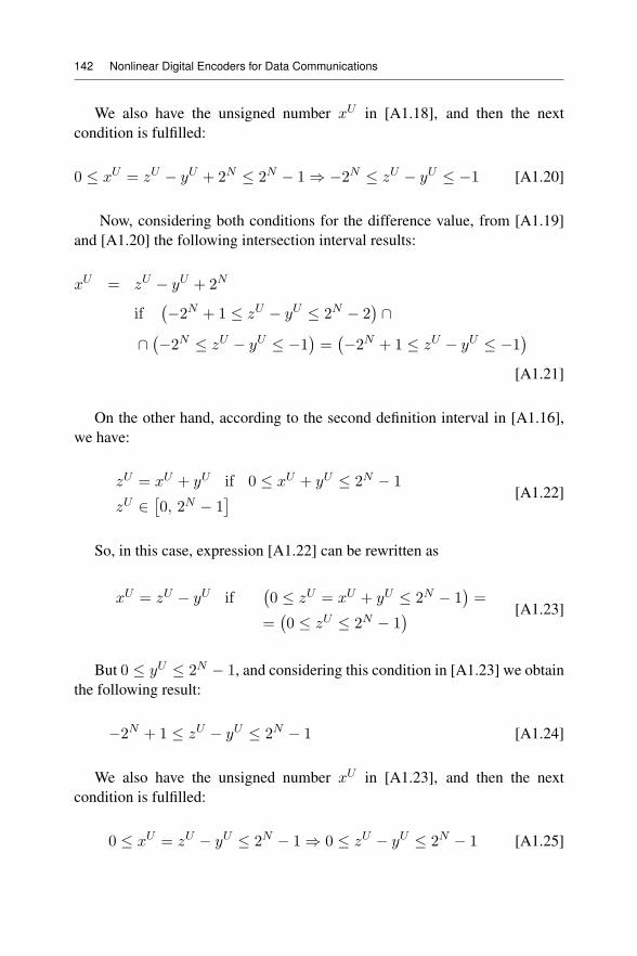
142 Nonlinear Digital Encoders for Data Communications
We also have the unsigned number xU in [A1.18], and then the nextcondition is fulfilled:
0 ≤ xU = zU − yU + 2N ≤ 2N − 1 ⇒ −2N ≤ zU − yU ≤ −1 [A1.20]
Now, considering both conditions for the difference value, from [A1.19]and [A1.20] the following intersection interval results:
xU = zU − yU + 2N
if −2N + 1 ≤ zU − yU ≤ 2N − 2 ∩∩ −2N ≤ zU − yU ≤ −1 = −2N + 1 ≤ zU − yU ≤ −1
[A1.21]
On the other hand, according to the second definition interval in [A1.16],we have:
zU = xU + yU if 0 ≤ xU + yU ≤ 2N − 1
zU ∈ 0, 2N − 1[A1.22]
So, in this case, expression [A1.22] can be rewritten as
xU = zU − yU if 0 ≤ zU = xU + yU ≤ 2N − 1 =
= 0 ≤ zU ≤ 2N − 1[A1.23]
But 0 ≤ yU ≤ 2N − 1, and considering this condition in [A1.23] we obtainthe following result:
−2N + 1 ≤ zU − yU ≤ 2N − 1 [A1.24]
We also have the unsigned number xU in [A1.23], and then the nextcondition is fulfilled:
0 ≤ xU = zU − yU ≤ 2N − 1 ⇒ 0 ≤ zU − yU ≤ 2N − 1 [A1.25]
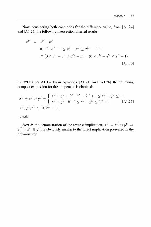
Appendix 143
Now, considering both conditions for the difference value, from [A1.24]and [A1.25] the following intersection interval results:
xU = zU − yU
if −2N + 1 ≤ zU − yU ≤ 2N − 1 ∩∩ 0 ≤ zU − yU ≤ 2N − 1 = 0 ≤ zU − yU ≤ 2N − 1
[A1.26]
CONCLUSION A1.1.– From equations [A1.21] and [A1.26] the followingcompact expression for the operator is obtained:
xU = zU yU =zU − yU + 2N if −2N + 1 ≤ zU − yU ≤ −1
zU − yU if 0 ≤ zU − yU ≤ 2N − 1
xU , yU , zU ∈ 0, 2N − 1
[A1.27]
q.e.d.
Step 2: the demonstration of the reverse implication, xU = zU yU ⇒zU = xU ⊕ yU , is obviously similar to the direct implication presented in theprevious step.

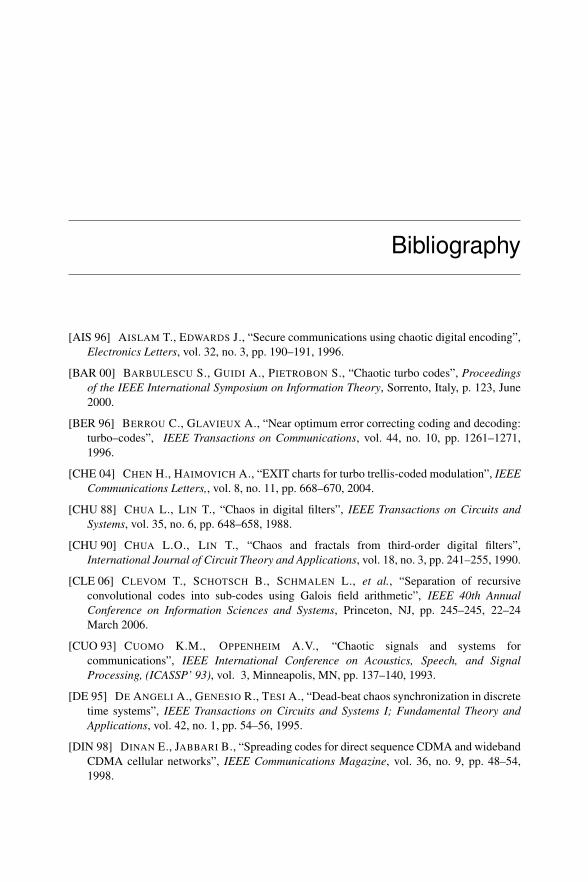
Bibliography
[AIS 96] AISLAM T., EDWARDS J., “Secure communications using chaotic digital encoding”,Electronics Letters, vol. 32, no. 3, pp. 190–191, 1996.
[BAR 00] BARBULESCU S., GUIDI A., PIETROBON S., “Chaotic turbo codes”, Proceedingsof the IEEE International Symposium on Information Theory, Sorrento, Italy, p. 123, June2000.
[BER 96] BERROU C., GLAVIEUX A., “Near optimum error correcting coding and decoding:turbo–codes”, IEEE Transactions on Communications, vol. 44, no. 10, pp. 1261–1271,1996.
[CHE 04] CHEN H., HAIMOVICH A., “EXIT charts for turbo trellis-coded modulation”, IEEECommunications Letters,, vol. 8, no. 11, pp. 668–670, 2004.
[CHU 88] CHUA L., LIN T., “Chaos in digital filters”, IEEE Transactions on Circuits andSystems, vol. 35, no. 6, pp. 648–658, 1988.
[CHU 90] CHUA L.O., LIN T., “Chaos and fractals from third-order digital filters”,International Journal of Circuit Theory and Applications, vol. 18, no. 3, pp. 241–255, 1990.
[CLE 06] CLEVOM T., SCHOTSCH B., SCHMALEN L., et al., “Separation of recursiveconvolutional codes into sub-codes using Galois field arithmetic”, IEEE 40th AnnualConference on Information Sciences and Systems, Princeton, NJ, pp. 245–245, 22–24March 2006.
[CUO 93] CUOMO K.M., OPPENHEIM A.V., “Chaotic signals and systems forcommunications”, IEEE International Conference on Acoustics, Speech, and SignalProcessing, (ICASSP’ 93), vol. 3, Minneapolis, MN, pp. 137–140, 1993.
[DE 95] DE ANGELI A., GENESIO R., TESI A., “Dead-beat chaos synchronization in discretetime systems”, IEEE Transactions on Circuits and Systems I; Fundamental Theory andApplications, vol. 42, no. 1, pp. 54–56, 1995.
[DIN 98] DINAN E., JABBARI B., “Spreading codes for direct sequence CDMA and widebandCDMA cellular networks”, IEEE Communications Magazine, vol. 36, no. 9, pp. 48–54,1998.
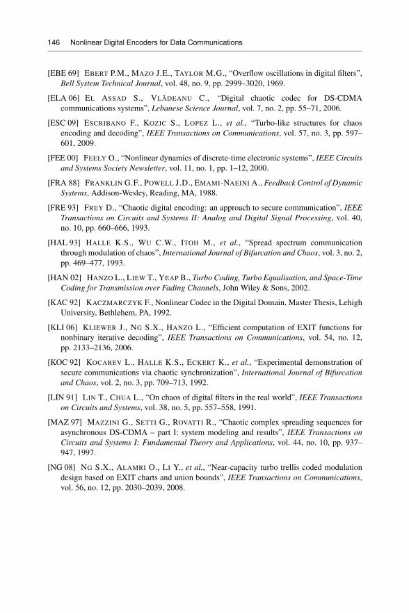
146 Nonlinear Digital Encoders for Data Communications
[EBE 69] EBERT P.M., MAZO J.E., TAYLOR M.G., “Overflow oscillations in digital filters”,Bell System Technical Journal, vol. 48, no. 9, pp. 2999–3020, 1969.
[ELA 06] EL ASSAD S., VLADEANU C., “Digital chaotic codec for DS-CDMAcommunications systems”, Lebanese Science Journal, vol. 7, no. 2, pp. 55–71, 2006.
[ESC 09] ESCRIBANO F., KOZIC S., LOPEZ L., et al., “Turbo-like structures for chaosencoding and decoding”, IEEE Transactions on Communications, vol. 57, no. 3, pp. 597–601, 2009.
[FEE 00] FEELY O., “Nonlinear dynamics of discrete-time electronic systems”, IEEE Circuitsand Systems Society Newsletter, vol. 11, no. 1, pp. 1–12, 2000.
[FRA 88] FRANKLIN G.F., POWELL J.D., EMAMI-NAEINI A., Feedback Control of DynamicSystems, Addison-Wesley, Reading, MA, 1988.
[FRE 93] FREY D., “Chaotic digital encoding: an approach to secure communication”, IEEETransactions on Circuits and Systems II: Analog and Digital Signal Processing, vol. 40,no. 10, pp. 660–666, 1993.
[HAL 93] HALLE K.S., WU C.W., ITOH M., et al., “Spread spectrum communicationthrough modulation of chaos”, International Journal of Bifurcation and Chaos, vol. 3, no. 2,pp. 469–477, 1993.
[HAN 02] HANZO L., LIEW T., YEAP B., Turbo Coding, Turbo Equalisation, and Space-TimeCoding for Transmission over Fading Channels, John Wiley & Sons, 2002.
[KAC 92] KACZMARCZYK F., Nonlinear Codec in the Digital Domain, Master Thesis, LehighUniversity, Bethlehem, PA, 1992.
[KLI 06] KLIEWER J., NG S.X., HANZO L., “Efficient computation of EXIT functions fornonbinary iterative decoding”, IEEE Transactions on Communications, vol. 54, no. 12,pp. 2133–2136, 2006.
[KOC 92] KOCAREV L., HALLE K.S., ECKERT K., et al., “Experimental demonstration ofsecure communications via chaotic synchronization”, International Journal of Bifurcationand Chaos, vol. 2, no. 3, pp. 709–713, 1992.
[LIN 91] LIN T., CHUA L., “On chaos of digital filters in the real world”, IEEE Transactionson Circuits and Systems, vol. 38, no. 5, pp. 557–558, 1991.
[MAZ 97] MAZZINI G., SETTI G., ROVATTI R., “Chaotic complex spreading sequences forasynchronous DS-CDMA – part I: system modeling and results”, IEEE Transactions onCircuits and Systems I: Fundamental Theory and Applications, vol. 44, no. 10, pp. 937–947, 1997.
[NG 08] NG S.X., ALAMRI O., LI Y., et al., “Near-capacity turbo trellis coded modulationdesign based on EXIT charts and union bounds”, IEEE Transactions on Communications,vol. 56, no. 12, pp. 2030–2039, 2008.
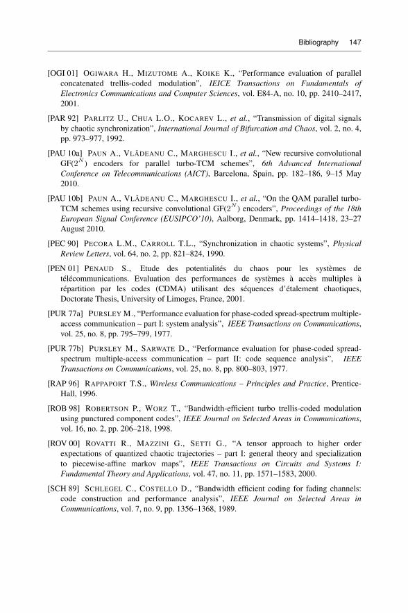
Bibliography 147
[OGI 01] OGIWARA H., MIZUTOME A., KOIKE K., “Performance evaluation of parallelconcatenated trellis-coded modulation”, IEICE Transactions on Fundamentals ofElectronics Communications and Computer Sciences, vol. E84-A, no. 10, pp. 2410–2417,2001.
[PAR 92] PARLITZ U., CHUA L.O., KOCAREV L., et al., “Transmission of digital signalsby chaotic synchronization”, International Journal of Bifurcation and Chaos, vol. 2, no. 4,pp. 973–977, 1992.
[PAU 10a] PAUN A., VLADEANU C., MARGHESCU I., et al., “New recursive convolutionalGF(2N ) encoders for parallel turbo-TCM schemes”, 6th Advanced InternationalConference on Telecommunications (AICT), Barcelona, Spain, pp. 182–186, 9–15 May2010.
[PAU 10b] PAUN A., VLADEANU C., MARGHESCU I., et al., “On the QAM parallel turbo-TCM schemes using recursive convolutional GF(2N ) encoders”, Proceedings of the 18thEuropean Signal Conference (EUSIPCO’10), Aalborg, Denmark, pp. 1414–1418, 23–27August 2010.
[PEC 90] PECORA L.M., CARROLL T.L., “Synchronization in chaotic systems”, PhysicalReview Letters, vol. 64, no. 2, pp. 821–824, 1990.
[PEN 01] PENAUD S., Etude des potentialités du chaos pour les systèmes detélécommunications. Evaluation des performances de systèmes à accès multiples àrépartition par les codes (CDMA) utilisant des séquences d’étalement chaotiques,Doctorate Thesis, University of Limoges, France, 2001.
[PUR 77a] PURSLEY M., “Performance evaluation for phase-coded spread-spectrum multiple-access communication – part I: system analysis”, IEEE Transactions on Communications,vol. 25, no. 8, pp. 795–799, 1977.
[PUR 77b] PURSLEY M., SARWATE D., “Performance evaluation for phase-coded spread-spectrum multiple-access communication – part II: code sequence analysis”, IEEETransactions on Communications, vol. 25, no. 8, pp. 800–803, 1977.
[RAP 96] RAPPAPORT T.S., Wireless Communications – Principles and Practice, Prentice-Hall, 1996.
[ROB 98] ROBERTSON P., WORZ T., “Bandwidth-efficient turbo trellis-coded modulationusing punctured component codes”, IEEE Journal on Selected Areas in Communications,vol. 16, no. 2, pp. 206–218, 1998.
[ROV 00] ROVATTI R., MAZZINI G., SETTI G., “A tensor approach to higher orderexpectations of quantized chaotic trajectories – part I: general theory and specializationto piecewise-affine markov maps”, IEEE Transactions on Circuits and Systems I:Fundamental Theory and Applications, vol. 47, no. 11, pp. 1571–1583, 2000.
[SCH 89] SCHLEGEL C., COSTELLO D., “Bandwidth efficient coding for fading channels:code construction and performance analysis”, IEEE Journal on Selected Areas inCommunications, vol. 7, no. 9, pp. 1356–1368, 1989.
148 Nonlinear Digital Encoders for Data Communications
[SCH 03] SCHRECKENBACH F., GORTZ N., HAGENAUER J., et al., “Optimized symbolmappings for bit-interleaved coded modulation with iterative decoding”, IEEE GlobalTelecommunications Conference (GLOBECOM ’03), vol. 6, San Francisco, pp. 3316–3320,1–5 December 2003.
[TEN 01] TEN BRINK S., “Convergence behavior of iteratively decoded parallel concatenatedcodes”, IEEE Transactions on Communications, vol. 49, no. 10, pp. 1727–1737, 2001.
[TES 94] TESI A., DE ANGELI A., GENESIO R., “On the system decomposition forsynchronizing chaos”, International Journal of Bifurcation and Chaos, vol. 4, no. 6,pp. 1675–1685, 1994.
[UNG 82] UNGERBOECK G., “Channel coding with multilevel/phase signals”, IEEETransactions on Information Theory, vol. IT-28, no. 1, pp. 55–67, 1982.
[VLA 09a] VLADEANU C., EL ASSAD S., CARLACH J.-C., et al., “Improved Frey chaoticdigital encoder for trellis-coded modulation”, IEEE Transactions on Circuits and SystemsII: Express Briefs, vol. 56, no. 6, pp. 509–513, 2009.
[VLA 09b] VLADEANU C., EL ASSAD S., CARLACH J.-C., et al., “Optimum PAM-TCMschemes using left-circulate function over GF(2N )”, International Symposium on Signals,Circuits and Systems (ISSCS 09), Iasi, Romania, pp. 267–270, 9–10 July 2009.
[VLA 09c] VLADEANU C., EL ASSAD S., CARLACH J.-C., et al., “Chaotic digitalencoding for 2D trellis-coded modulation”, 5th Advanced International Conference onTelecommunications (AICT’ 09), Venice, Italy, pp. 152–157, 24–28 May 2009.
[VLA 10a] VLADEANU C., PAUN A., LUCACIU R., et al., “Parallel turbo-TCM schemesusing recursive convolutional GF(2N ) encoders over frequency non-selective fadingchannel”, 9th International Symposium on Electronics and Telecommunications (ISETC’10), Timisoara, Romania, pp. 285–288, 11–12 November 2010.
[VLA 10b] VLADEANU C., EL ASSAD S., CARLACH J.-C., et al., “Recursive GF(2N )encoders using left-circulate function for optimum PSK-TCM schemes”, Signal Processing,vol. 90, no. 9, pp. 2708–2713, 2010.
[VLA 11a] VLADEANU C., EL ASSAD S., “Designing optimum 2D-TCM schemes usingnew systematic convolutional encoders over GF(2N )”, 10th International Symposium onSignals, Circuits and Systems (ISSCS ’11), Iasi, Romania, pp. 479–483, 30 June–1 July2011.
[VLA 11b] VLADEANU C., EL ASSAD S., “Optimum QAM-TCM schemes using left-circulate function over GF(2N )”, IEEE 7th Advanced International Conference onTelecommunication (AICT ’11), St. Maarten, the Netherlands, pp. 112–116, 20–25 March2011.
[VLA 11c] VLADEANU C., EL ASSAD S., “Punctured 8-PSK turbo-TCM transmissionsusing recursive systematic convolutional GF(2N ) encoders”, Proceedings of the 19thEuropean Signal Conference (EUSIPCO ’11), Barcelona, Spain, pp. 111–115, 29 August–2September 2011.
Bibliography 149
[VLA 12] VLADEANU C., MARTIAN A., EL ASSAD S., “EXIT Charts analysis for turbo-TCM schemes using non-binary RSC encoders”, IEEE 8th Advanced InternationalConference on Telecommunication (AICT ’12), Stuttgart, Germany, pp. 150–155, 27 May–1June 2012.
[VUC 00] VUCETIC B., YUAN J., Turbo Codes: Principles and Applications, Springer, 2000.
[WER 98] WERTER M., “An improved chaotic digital encoder”, IEEE Transactions onCircuits and Systems II: Analog and Digital Signal Processing, vol. 45, no. 2, pp. 227–229, 1998.
[WU 93] WU C.W., CHUA L.O., “A simple way to synchronize chaotic systems withapplication to secure communications systems”, International Journal of Bifurcation andChaos, vol. 3, no. 6, pp. 1619–1627, 1993.
[ZHO 01] ZHOU X., LIU J., SONG W., et al., “Chaotic turbo codes in secure communication”,International Conference on Trends in Communications (EUROCON ’01), vol. 1,Bratislava, Slovakia, pp. 199–201, 5–7 July 2001.

Index
2’s complement operators,10, 30
C, D, E, F
chaotic spreading sequences,15, 16dead-beat sequencesynchronization,19, 23–26, 43–45
Euclidean distance, 49–51, 54, 57,59, 63, 67, 70, 71, 78, 80, 85
extrinsic information transfer (EXIT)chart, 114
Frey encoder, 9, 29, 38, 50, 53, 54,58, 61, 65, 78trellis design, 54,
G, L, M, N
generalized optimum recursiveconvolutional LCIRC (RC-LCIRC)encoder, 87, 88, 90, 97, 98, 116
left-circulate (LCIRC) function, 29,50
log likelihood ratio (LLR), 98minimum effective length, 107, 125minimum product distance, 107modulo operators; 29nonlinear digital encoders, 1, 49, 97,115
P, Q, R
properties of the LCIRC function, 38punctured TTCM scheme with RSC-LCIRC encoders, 97, 105, 109,123–126
quasi-chaotic sequences, 5RC-LCIRC encoder for parallelTTCM scheme, 97
recursive and systematicconvolutional LCIRC (RSC-LCIRC) encoder, 56, 100
S, T
simulated bit error rate (BER), 15,115
simulated symbol error rate (SER),45, 119
Simulink implementation of Freycodec, 45,
symbol-by-symbol logarithmicmaximum a-posteriori probability(log-MAP) iterative decoder, 112
TCM encoders for PAM, PSK, andQAM, 108
trellis-coded modulation (TCM), 54turbo-TCM (TTCM), 98, 99, 116–120