nonlinear and non-gaussian state space modeling using
TRANSCRIPT

Ann. Inst. Statist. Math.
Vol. 53, No. 1, 63–81 (2001)
NONLINEAR AND NON-GAUSSIAN STATE SPACE MODELING USING
SAMPLING TECHNIQUES
Hisashi Tanizaki*
Faculty of Economics, Kobe University, Kobe 657-5801, Japan
(Received April 11, 2000; Revised October 12, 2000)
Abstract. In this paper, the nonlinear non-Gaussian filters and smoothers whichare much less computational than the existing ones are proposed, where the sam-pling techniques such as rejection sampling (RS), importance resampling (IR) and theMetropolis-Hastings independence sampling (MH) are utilized. The existing density-based nonlinear and non-Gaussian filters and smoothers utilize the marginal densities,i.e., p(αt|Yt) for filtering and p(αt|YT ) for smoothing, but the algorithms proposedin this paper are based on the joint densities, i.e., p(αt, αt−1|Yt) for filtering andp(αt+1, αt|YT ) or p(αt+1, αt, αt−1|YT ) for smoothing. That is, in this paper, the ran-dom draws of αt are generated from p(αt, αt−1|Yt) for filtering and p(αt+1, αt|YT ) orp(αt+1, αt, αt−1|YT ) for smoothing. By generating the random draws from the jointdensities, much less computer-intensive algorithms on filtering and smoothing canbe obtained. Furthermore, taking into account possibility of structural changes andoutliers during the estimation period, the appropriately chosen sampling density ispossibly introduced into the suggested nonlinear non-Gaussian filtering and smooth-ing procedures. Finally, through Monte Carlo simulation studies, the suggested filtersand smoothers are examined.
Key words and phrases: State Space Modeling, Filtering, Smoothing, MarginalDensity, Joint Density, Rejection Sampling, Importance Resampling, Metropolis-Hastings Independence Sampling.
1. Introduction
Various nonlinear non-Gaussian filters and smoothers have been proposed for thelast decade in order to improve precision of the state estimates and reduce a computa-tional burden. The state mean and variance are evaluated by generating random drawsdirectly from the filtering density or the smoothing density. Clearly, precision of thestate estimates is improved as number of random draws increases. Thus, the recent fil-ters and smoothers have been developed by applying some sampling techniques such asGibbs sampling, rejection sampling (RS), importance resampling (IR), the Metropolis-Hastings independence sampling (MH) and etc.
Carlin et al. (1992) and Carter and Kohn (1994, 1996) applied the Gibbs samplerto some specific state space models, which are extended to more general state spacemodels by Geweke and Tanizaki (1999). The Gibbs sampler sometimes gives us the
*The author would like to acknowledge the constructive comments of the anonymous referees. This
research was partially supported by the Ministry of Education, Science, Sports and Culture, Grant-in-
Aid for Encouragement of Young Scientists (# 12730022).
1
2
imprecise estimates of the state variables, depending on the underlying state space model(see Carter and Kohn (1994, 1996)). Especially when the random variables are highlycorrelated with each other, it is well known that convergence of the Gibbs sampler isunacceptably slow. In the case of state space models, the transition equation representsthe relationship between the state variable αt and the lagged one αt−1. Accordingly, itis clear that the state variable at present time has high correlation with that at pasttime. As for the state space models, therefore, the Gibbs sampler is one of the sourcesof imprecise state estimates. In this paper, unlike Carlin et al. (1992) and Carter andKohn (1994, 1996), the density-based recursive algorithms on filtering and smoothingare discussed, where they are compared with respect to the three sampling methods, i.e.,RS, IR and MH, although any sampling technique can be applied.
Gordon et al. (1993), Kitagawa (1996, 1998) and Kitagawa and Gersch (1996) pro-posed the nonlinear non-Gaussian state space modeling by IR, which can be applied toalmost all the state space models. Both filtering and smoothing random draws are basedon the one-step ahead prediction random draws. In the case where the past informationis too different from the present sample, however, the obtained filtering and smoothingrandom draws become unrealistic. To avoid this situation, in this paper we take an ap-propriately chosen density as the sampling density for random number generation. Notethat Kong et al. (1994), Liu and Chen (1995, 1998) and Doucet et al. (2000) also utilizedthe density other than the state estimation. In addition, the fixed-interval smoother pro-posed by Kitagawa (1996) and Kitagawa and Gersch (1996) does not give us the exactsolution of the state estimate even when the number of random draws is large enough,because the fixed-interval smoother suggested by Kitagawa (1996) is approximated bythe fixed-lag smoother. To improve these disadvantages, in this paper we propose thefixed-interval smoother which yields the exact solution of the state estimate. As analternative smoother, furthermore, Kitagawa (1996) introduces the fixed-lag smootherbased on the two-filter formula, where forward and backward filtering are performed andcombined to obtain the smoothing density. The smoother based on the two-filter formulais discussed in Appendix A.
Moreover, the RS filter and smoother have been developed by Tanizaki (1996, 1999),Hurzeler and Kunsch (1998) and Tanizaki and Mariano (1998). To implement RS forrandom number generation, we need to compute the supremum in the acceptance prob-ability, which depends on the underlying functional form of the measurement and tran-sition equations. RS cannot be applied in the case where the acceptance probability isequal to zero, i.e., when the supremum is infinity. Even if the supremum is finite, ittakes a lot of computational time when the acceptance probability is close to zero. Toimprove the problems in rejection sampling, Liu, Chen and Wong (1998) suggested therejection controlled sequential importance sampling algorithm, where rejection samplingand importance sampling are combined.
As computer progresses day by day, the computer-intensive nonlinear non-Gaussianestimators have been developed. However, it is clear that less computational estimatorsare preferred. To reduce the computational disadvantages for filtering and smoothing, weconsider generating random draws from the joint densities (i.e., p(αt, αt−1|Yt) for filteringand p(αt+1, αt|YT ) or p(αt+1, αt, αt−1|YT ) for smoothing, where the notations are definedin Section 2.1), not from the marginal densities (i.e., p(αt|Yt) for filtering and p(αt|YT )for smoothing). A lot of filters have been proposed based on the marginal density andaccordingly the existing filters are computationally too intensive. Kong et al. (1994)and Liu and Chen (1995) also suggested drawing from the joint density of the state

3
variable and the auxiliary variable. However, use of the auxiliary variable yields a verycomputer-intensive filtering algorithm. Therefore, for filtering, we consider drawing fromthe joint density of the state variables, i.e., (αt, αt−1), given Yt. Furthermore, in a lot ofliterature on the IR and RS procedures, smoothing is not investigated because smoothingis much more computer-intensive than filtering. Dealing with the joint densities of thestate variables yields less computational procedures and therefore we can obtain not onlyfiltering but also smoothing in the IR and RS procedures. In this paper, thus, we proposemuch less computational nonlinear non-Gaussian filters and smoothers using the jointdensities of the state variables, where RS, IR or MH may be utilized for random numbergeneration.
2. Preliminaries
2.1 State Space Model
Kitagawa (1987), Harvey (1989), Kitagawa and Gersch (1996) and Tanizaki (1996,2000) discuss the nonlinear non-Gaussian state space models, which are described by thefollowing two equations:
(Measurement equation) yt = ht(αt, εt),(2.1)
(Transition equation) αt = ft(αt−1, ηt),(2.2)
where yt represents the observed data at time t while αt denotes the state vector at timet which is unobservable. εt and ηt are mutually independently distributed. ht(·, ·) andft(·, ·) are assumed to be known. αt|s ≡ E(αt|Ys) is called prediction if t > s, filteringif t = s and smoothing if t < s, where Ys denotes the information set up to time s,i.e., Ys = y1, y2, · · · , ys. Moreover, there are three kinds of smoothing estimators, i.e.,the fixed-point smoothing αL|t, the fixed-lag smoothing αt|t+L and the fixed-intervalsmoothing αt|T for fixed L and fixed T . In this paper, we focus on the filter and thefixed-interval smoother, i.e., αt|s for s = t, T .
Define py(yt|αt) and pα(αt|αt−1) by the density functions derived from the mea-surement equation (2.1) and the transition equation (2.2). The density-based filteringalgorithm is given by:
(Prediction equation) p(αt|Yt−1) =
∫pα(αt|αt−1)p(αt−1|Yt−1)dαt−1,(2.3)
(Update equation) p(αt|Yt) =py(yt|αt)p(αt|Yt−1)∫
py(yt|αt)p(αt|Yt−1)dαt,(2.4)
for t = 1, 2, · · · , T . The initial condition is given by: p(α1|Y0) =∫
pα(α1|α0)pα(α0)dα0 ifα0 is stochastic and p(α1|Y0) = pα(α1|α0) otherwise. pα(α0) denotes the unconditionaldensity of α0. The filtering algorithm takes the following two steps: (i) from equation(2.3), p(αt|Yt−1) is obtained given p(αt−1|Yt−1), and (ii) from equation (2.4), p(αt|Yt) isderived given p(αt|Yt−1). Thus, p(αt|Yt) is recursively obtained for t = 1, 2, · · · , T .
The density-based smoothing algorithm utilizes both the one-step ahead predictiondensity p(αt+1|Yt) and the filtering density p(αt|Yt), which is represented by:
p(αt|YT ) = p(αt|Yt)
∫p(αt+1|YT )pα(αt+1|αt)
p(αt+1|Yt)dαt+1,(2.5)
4
for t = T − 1, T − 2, · · · , 1. Given p(αt|Yt) and p(αt+1|Yt), the smoothing algorithmrepresented by equation (2.5) is a backward recursion from p(αt+1|YT ) to p(αt|YT ).
For the fixed-interval smoother, Kitagawa (1996) developed an alternative smooth-ing algorithm, which is based on the two-filter formula. This alternative algorithm isdiscussed in Appendix A.
Let g(·) be a function, e.g., g(αt) = αt for mean or g(αt) = (αt − αt|s)(αt − αt|s)′
for variance. Given p(αt|Ys), the conditional expectation of g(αt) given Ys is representedby:
E(g(αt)|Ys
)=
∫g(αt)p(αt|Ys)dαt.(2.6)
When we have the unknown parameters in equations (2.1) and (2.2), the followinglikelihood function is maximized with respect to the parameters:
p(YT ) =T∏
t=1
p(yt|Yt−1) =T∏
t=1
(∫p(yt|αt)p(αt|Yt−1)dαt
).(2.7)
Since p(yt|Yt−1) in (2.7) corresponds to the denominator in equation (2.4), we do notneed extra computation for evaluation of the likelihood function. Thus, the unknownparameter is obtained by maximum likelihood estimation (MLE). As for an alternativeapproach to estimate the unknown parameter, Kitagawa (1998) suggested taking theunknown parameter as the state variable, which is called the self-organizing filter.
Our goal is to obtain the expectation in (2.6), which is evaluated generating randomdraws of αt. Therefore, in the next section, we overview some sampling techniques.
2.2 Sampling Techniques
We want to generate random draws from p(x), called the target density, but weconsider the case where it is hard to sample from p(x). Suppose that it is easy togenerate a random draw from another density p∗(x), called the sampling density. Inthis case, random draws of x from the target density p(x) are generated by utilizingthe random draws sampled from the sampling density p∗(x). Let xi be the i-th randomdraw of x generated from the target density p(x). We consider generating x1, x2, · · ·, xN
from the target density p(x). Suppose that q(x) is proportional to the ratio of the targetdensity and the sampling density, i.e., q(x) ∝ p(x)/p∗(x). Then, the target density isrewritten as: p(x) ∝ q(x)p∗(x).
Based on q(x), the acceptance probability is computed. The random draw is gener-ated from the sampling density p∗(x). Using the acceptance probability based on q(x),we can obtain the random draw from the target density p(x). Depending on the struc-ture of the acceptance probability, we have three kinds of sampling techniques, i.e., RS,IR and MH. Thus, to generate random draws of x from the target density p(x), thefunctional form of q(x) should be known and random draws have to be easily generatedfrom the sampling density p∗(x).
Now we discuss the three sampling techniques, which are the random number gen-eration methods in the case where it is not easy to generate random draws directly fromthe target density. See Liu (1996) for a comparison of the three sampling methods.For all the three sampling techniques, the sampling density p∗(x) is utilized, i.e., xi isgenerated through the sampling density p∗(x).

5
2.2.1 Rejection Sampling (RS)
Let x∗ be a random draw of x generated from the sampling density p∗(x). Definethe acceptance probability as: ω(x) = q(x)/ sup
zq(z), where the supremum is assumed
to be finite. N random draws of x from the target density p(x) are obtained as follows:(i) generate x∗ from the sampling density p∗(x) and compute ω(x∗), (ii) set xi = x∗
with probability ω(x∗) and go back to (i) otherwise, and (iii) repeat (i) and (ii) fori = 1, 2, · · · , N .
RS is the most efficient sampling method in the sense of precision of the randomdraws, because using RS we can generate mutually independently distributed randomdraws. However, in order to apply RS, we need to obtain the supremum of q(x). Ifthe supremum is infinite, the acceptance probability ω(x) is zero and accordingly thecandidate x∗ is never accepted in Steps (i) and (ii). Let NR be the average number ofthe rejected random numbers. We need 1 + NR random draws in average to generateone random number from the target density p(x). In other words, the rejection rate isgiven by 1/(1 + NR) in average. Therefore, to obtain N random draws from the targetdensity p(x), we have to generate N(1 + NR) random draws from the sampling densityp∗(x). See, for example, Boswell, Gore, Patil and Taillie (1993), O’Hagan (1994) andGeweke (1996) for rejection sampling.
To examine the condition that ω(x) is greater than zero, consider the case where p(x)and p∗(x) are distributed as N(µ, σ2) and N(µ∗, σ
2∗), respectively. Then, σ2
∗ > σ2 canbe derived for existence of the supremum, which implies that the sampling density p∗(x)should be more broadly distributed than the target density p(x). Thus, it is known thatRS has the disadvantages: we need to compute the supremum in ω(x), which sometimesdoes not exist, and it takes a long time in the case where ω(·) is close to zero even if thesupremum exists.
2.2.2 Importance Resampling (IR)
Let x∗i be the i-th random draw of x generated from the sampling density p∗(x). The
acceptance probability is defined as: ω(x∗i ) = q(x∗
i )/∑N
j=1 q(x∗j ). To obtain N random
draws from the target density p(x), we perform the following procedure: (i) generatex∗
j from the sampling density p∗(x) and compute ω(x∗j ) for all j = 1, 2, · · · , N , (ii) take
xi = x∗j with probability ω(x∗
j ), and (iii) repeat (ii) for i = 1, 2, · · · , N .
In Step (ii), practically we need to generate a uniform random draw between zeroand one, denoted by u, and set xi = x∗
j when Ωj−1 ≤ u < Ωj , where Ωj ≡ Ωj−1 + ω(x∗j )
and Ω0 ≡ 0. For example, see Smith and Gelfand (1992) for the resampling procedure.
For precision of the random draws, IR is inferior to RS under the assumption forRS that the supremum in the acceptance probability exists. According to IR, when wehave N different random draws from the sampling density, we pick up one of them withthe corresponding probability weight. Therefore, some of the random draws have theexactly same values for IR, while all the random draws take the different values for RS.In other words, to obtain N random draws from the target density p(x), IR requires justN random draws from the sampling density p∗(x), but RS needs more than N randomdraws from the sampling density p∗(x). Remember that in order for RS to generate onerandom draw from the target density p(x) we need one accepted random draw and somerejected random draws from the sampling density p∗(x).
2.2.3 Metropolis-Hastings Independence Sampling (MH)
Let us define the acceptance probability by: ω(xi−1, x∗) = min
(q(x∗)/q(xi−1), 1
). N
random draws of x from the target density p(x) are generated as: (i) take the initial value
6
of x as x−M , (ii) generate x∗ from the sampling density p∗(x) and compute ω(xi−1, x∗),
(iii) set xi = x∗ with probability ω(xi−1, x∗) and xi = xi−1 otherwise, and (iv) repeat
(ii) and (iii) for i = −M + 1,−M + 2, · · · , N .For choice of the sampling density p∗(x), the sampling density should not have too
large variance and too small variance, compared with the target density. The samplingdensity p∗(x) should be chosen so that the chain travels over the support of the targetdensity p(x). It is also possible to take p∗(x
∗) = p∗(x∗|xi−1). See, for example, Chib
and Greenberg (1995) and Geweke (1996) for MH.Note as follows. For MH, x1 is taken as a random draw of x from the target density
p(x) for sufficiently large M . To obtain N random draws, thus we need to generateM + N random draws. Moreover, clearly we have Cov(xi−1, xi) > 0, because xi isgenerated based on xi−1. Therefore, for precision of the random draws, MH gives us theworst random number of the three sampling methods.
As an alternative random number generation method to avoid the positive correla-tion, we can perform the case of N = 1 in the above procedures (i) – (iv) N times inparallel, taking different initial values for x−M . In this case, we need to generate M + 1random numbers to obtain one random draw from the target density p(x). That is, Nrandom draws from the target density p(x) are based on N(1 + M) random draws fromthe sampling density p∗(x). Thus, we can obtain mutually independently distributedrandom draws. For precision of the random draws, the alternative MH is similar to RS.However, this alternative method is too computer-intensive, compared with the aboveprocedures (i) – (iv), which takes more time RS in the case of M > NR. In simulationstudies of Section 4., we do not utilize this alternative MH.
3. Use of the Sampling Techniques
As discussed in Section 2.2, in order to apply the sampling techniques, the filteringdensity and the smoothing density have to be written as the form p(x) ∝ q(x)p∗(x),where q(x) is the known function and p∗(x) denotes the sampling density.
Let αi,t|s be the i-th random draw of αt from p(αt|Ys). Using the sampling tech-niques such as RS, IR and MH, in this section we consider generating αi,t|s. If therandom draws (α1,t|s, α2,t|s, · · ·, αN,t|s) for s = t, T and t = 1, 2, · · · , T are available,
equation (2.6) is evaluated by E(g(αt)|Ys
)≈ (1/N)
∑Ni=1 g(αi,t|s). Similarly, equation
(2.7) is given by:
p(YT ) ≈T∏
t=1
(1
N
N∑
i=1
p(yt|αi,t|t−1)
),(3.8)
where αi,t|t−1 = ft(αi,t−1|t−1, ηi,t) and ηi,t denotes the i-th random draw of ηt. Utilizingequation (3.8), MLE is performed for estimation of the unknown parameter.
3.1 FilteringBased on (α1,t−1|t−1, α2,t−1|t−1, · · ·, αN,t−1|t−1), an attempt is made to generate
(α1,t|t, α2,t|t, · · ·, αN,t|t). Depending on whether the initial value α0 is stochastic or not,αi,0|0 for i = 1, 2, · · · , N are assumed to be generated from pα(α0) or to be fixed for alli.
We have two representations on the filtering density (2.4). First, as shown fromequation (2.4), p(αt|Yt) is immediately rewritten as follows:
p(αt|Yt) ∝ q1(αt)p(αt|Yt−1),(3.9)
7
where q1(αt) is given by:q1(αt) ∝ py(yt|αt).
In this case, p∗(x) and q(x) in Section 2.2 correspond to p(αt|Yt−1) and q1(αt), respec-tively. q1(αt) is known because py(yt|αt) is obtained from the measurement equation(2.1), and given αi,t−1|t−1 for i = 1, 2, · · · , N a random draw of αt from p(αt|Yt−1) iseasily generated through the transition equation (2.2). Accordingly, using the samplingtechniques shown in Section 2.2, αi,t|t can be generated based on αi,t|t−1. Note thatGordon et al. (1993), Kitagawa (1996, 1998) and Kitagawa and Gersch (1996) proposedthe IR filter based on (3.9).
When we have a structural change or an outlier at time t, the present sample p(yt|αt)is far from the one-step ahead prediction density p(αt|Yt−1). In this case, for IR and MHthe random draws of αt from p(αt|Yt) become unrealistic because the reasonable randomdraws of αt cannot be obtained from the sampling density p(αt|Yt−1), and for RS it takesa lot of time computationally because the acceptance probability becomes very small.In addition, when a random draw of ηt is not easily obtained, it might be difficult togenerate a random draw of αt from p(αt|Yt−1). As for the second representation of thefiltering density, therefore, we explicitly introduce the importance sampling density ofαt, i.e., p∗(αt|αt−1), to obtain more plausible random draws. Furthermore, to reducecomputational disadvantages, we consider generating random draws of αt from the jointdensity p(αt, αt−1|Yt). Substituting equation (2.3) into equation (2.4) and eliminatingthe integration with respect to αt−1, the joint density of αt and αt−1 given Yt, i.e.,p(αt, αt−1|Yt), is written as:
p(αt, αt−1|Yt) ∝ q2(αt, αt−1)p∗(αt|αt−1)p(αt−1|Yt−1),(3.10)
where q2(αt, αt−1) is represented by:
q2(αt, αt−1) ∝py(yt|αt)pα(αt|αt−1)
p∗(αt|αt−1).
In equation (3.10), p∗(αt|αt−1)p(αt−1|Yt−1) is taken as the sampling density. WhenN random draws of αt−1 given Yt−1, i.e., αi,t−1|t−1 for i = 1, 2, · · · , N , are available,generating a random draw of αt−1 from p(αt−1|Yt−1) is equivalent to choosing oneout of the N random draws (α1,t−1|t−1, α2,t−1|t−1, · · ·, αN,t−1|t−1) with equal prob-ability weight. Given αi,t−1|t−1, a random draw of αt (i.e., α∗
i,t) is generated fromp∗(αt|αi,t−1|t−1). Thus, since the functional form of q2(αt, αt−1) is known and the ran-dom draw of (αt, αt−1) is generated from the sampling density p∗(αt|αt−1)p(αt−1|Yt−1),the random draws of (αt, αt−1) from the target density p(αt, αt−1|Yt) can be obtainedthrough RS, IR or MH. The i-th random draw of (αt, αt−1) from p(αt, αt−1|Yt) is de-noted by (αi,t|t, αi,t−1|t). The random draw which we want at this stage is αi,t|t, notαi,t−1|t. Note that a random draw of αt from p(αt, αt−1|Yt) is equivalent to that ofαt from p(αt|Yt). Furthermore, we point out that the appropriately chosen samplingdensity might be taken as p∗(αt|αt−1) = p∗(αt), which does not depend on αt−1.
To obtain the marginal density p(αt|Yt) based on (3.10), we have to integrate (3.10)with respect to αt−1. The marginal density p(αt|Yt) based on (3.10) reduces to p(αt|Yt) ∝
(1/N)∑N
j=1 q2(αt, αj,t−1|t−1)p∗(αt|αj,t−1|t−1). Therefore, random number generationfrom the marginal density p(αt| Yt) based on (3.10) is N times as computer-intensiveas that from the joint density p(αt, αt−1|Yt). This approach is adopted in numerous
8
literature, e.g., Hurzeler and Kunsch (1998), Liu and Chen (1998), Tanizaki (1996, 1999,2000) and Tanizaki and Mariano (1998). Clearly, use of p(αt, αt−1|Yt) leads to muchreduction in computational burden, rather than evaluation of
∫p(αt, αt−1|Yt)dαt−1. For
RS, we need to compute the supremum of q2 with respect to αt and αt−1. Therefore,sometimes, RS is not feasible if (3.10) is utilized. For (3.10), IR or MH is recommended,rather than RS.
3.2 SmoothingGiven (α1,t+1|T , α2,t+1|T , · · ·, αN,t+1|T ), we consider generating (α1,t|T , α2,t|T , · · ·,
αN,t|T ). Note that the smoothing random draws at time T are equivalent to the filteringrandom draws at time T , where both are represented by αi,T |T .
Based on equation (2.5), we have three representations on the smoothing density.By eliminating the integration with respect to αt+1 from equation (2.5), the first andsecond representations of p(αt+1, αt|YT ) are as follows:
p(αt+1, αt|YT ) ∝ q3(αt+1, αt)p(αt|Yt)p(αt+1|YT )(3.11)
∝ q4(αt+1, αt)p(αt|Yt−1)p(αt+1|YT ),(3.12)
where q3 and q4 are represented by:
q3(αt+1, αt) ∝pα(αt+1|αt)
p(αt+1|Yt),
q4(αt+1, αt) ∝ q1(αt)q3(αt+1, αt) ∝py(yt|αt)pα(αt+1|αt)
p(αt+1|Yt).
In equation (3.12), p(αt|Yt) in equation (3.11) is replaced by equation (3.9). For evalu-ation of p(αt+1|Yt) in q3(αt+1, αt) and q4(αt+1, αt) of equations (3.11) and (3.12), fromequation (2.3) we can use the following Monte Carlo integration:
p(αt+1|Yt) =
∫pα(αt+1|αt)p(αt|Yt)dαt(3.13)
≈1
N ′
N ′∑
j=1
pα(αt+1|αj,t|t),
where N ′ is not necessarily equal to N . To reduce the computational disadvantage, itmight be appropriate for N ′ to take the number which is less than N . Because α1,t|t,α2,t|t, · · ·, αN,t|t are in random order, the first N ′ random draws may be chosen forevaluation of the integration in equation (3.13). In any case, smoothing is N ′ times ascomputer-intensive as filtering, because of evaluation of p(αt+1|Yt). Thus, at each timeperiod t, the order of computation is given by N × N ′ for smoothing (remember thatthe order of computation is N for filtering).
In equation (3.11), the sampling density is given by p(αt+1|YT )p(αt|Yt). That is,the random draw of αt is sampled from p(αt|Yt), while that of αt+1 is from p(αt+1|YT ).Similarly, in equation (3.12), the sampling density becomes p(αt+1|YT )p(αt|Yt−1). Thus,(3.11) is different from (3.12) with respect to the sampling density of αt, i.e., the formeris based on p(αt|Yt) while the latter is p(αt|Yt−1). From equation (3.11) or (3.12), wecan generate the random draw of (αt+1, αt) from p(αt+1, αt|YT ), which is denoted by(αi,t+1|T , αi,t|T ). The random draw which we need at this stage is αi,t|T because we
9
already have αi,t+1|T . Thus, given (α1,t+1|T , α2,t+1|T , · · ·, αN,t+1|T ), αi,t|T is generated.Repeating the procedure for i = 1, 2, · · · , N , we can obtain (α1,t|T , α2,t|T , · · ·, αN,t|T ) bythe backward recursion.
Again, we compare the marginal density p(αt|YT ) and the joint density p(αt+1, αt|YT ) from computational point of view. Random number generation from p(αt|YT ) yieldsN times more computational burden than that from p(αt+1, αt|YT ) shown in equa-
tion (3.11) or (3.12), because we have to compute p(αt|YT ) ∝ (1/N)∑N
j=1 q3(αj,t+1|T ,
αt)p(αt|Yt) from equation (3.11) and p(αt|YT ) ∝ (1/N)∑N
j=1 q4(αj,t+1|T , αt)p(αt|Yt−1)from equation (3.12). Therefore, use of p(αt+1, αt|YT ) is much less computer-intensivethan that of p(αt|YT ).
In general, filtering is approximately close to smoothing when t approaches T (i.e.,the end point), because Yt approaches YT as t goes to T . Therefore, in order to obtain thesmoothing random draws around the end point, it might be plausible to take p(αt|Yt) for(3.11) and p(αt|Yt−1) for (3.12) as the sampling density of αt. However, when t goes tothe starting point, possibly p(αt|Yt) or p(αt|Yt−1) is quite different from p(αt|YT ). In thethird representation, therefore, another sampling density p∗(αt|αt−1, αt+1) is introducedto improve the smoothing random draws especially around the starting point. Substitut-ing equation (2.3) into equation (2.5) and eliminating the two integrations with respect toαt+1 and αt−1, the joint density of αt+1, αt and αt−1 given YT , i.e., p(αt+1, αt, αt−1|YT ),is obtained as:
p(αt+1, αt, αt−1|YT )(3.14)
∝ q5(αt+1, αt, αt−1)p(αt−1|Yt−1)p∗(αt|αt−1, αt+1)p(αt+1|YT ),
where q5 is given by:
q5(αt+1, αt, αt−1) ∝py(yt|αt)pα(αt|αt−1)pα(αt+1|αt)
p∗(αt|αt−1, αt+1)p(αt+1|Yt).
In equation (3.14), the sampling density is taken as p(αt+1|YT )p∗(αt|αt−1, αt+1)p(αt−1|Yt−1). After random draws of αt+1 and αt−1 are mutually independently generatedfrom p(αt+1|YT ) and p(αt−1|Yt−1), respectively, we may generate a random draw of αt
from another sampling density p∗(αt|αt−1, αt+1). That is, first, αi,t+1|T and αi,t−1|t−1
are generated from p(αt+1|YT ) and p(αt−1|Yt−1), and second, α∗i is generated from
p(αt|αi,t−1|t−1, αi,t+1|T ). Note that a random draw of αt from p(αt|YT ) is equivalentto that of αt from p(αt+1, αt, αt−1|YT ). That is, (αi,t+1|T , αi,t|T , αi,t−1|T ) is generatedfrom equation (3.14), but the random draw which we want is αi,t|T because αi,t+1|T
is already available and αi,t−1|T can be obtained at the next stage. Moreover, notethat p∗(αt|αt−1, αt+1) = p∗(αt) is also a possible candidate of the appropriately chosensampling density, where the sampling density is not a function of αt+1 and αt−1.
3.3 DiscussionBoth (3.9) and (3.10) are related to filtering while (3.11), (3.12) and (3.14) corre-
spond to smoothing. Using the sampling techniques such as RS, IR and MH, the randomdraws of αt are generated from (3.9) – (3.12) and (3.14). The correspondence betweenSections 2.2 and 3. is summarized in Table 1, where x denotes the random variable,p(x) is the target density and q(x) represents the ratio of the kernel and the samplingdensity (see Section 2.2). Our purpose is to generate random draws of αt from eachtarget density.

10
Table 1. Correspondence between Section 2.2 and Densities (3.9) – (3.12) and (3.14)
x p(x) q(x)
(3.9) αt p(αt|Yt) py(yt|αt)
(3.10) (αt, αt−1) p(αt, αt−1|Yt)py(yt|αt)pα(αt|αt−1)
p∗(αt|αt−1)
(3.11) (αt+1, αt) p(αt+1, αt|YT )pα(αt+1|αt)
p(αt+1|Yt)
(3.12) (αt+1, αt) p(αt+1, αt|YT )py(yt|αt)pα(αt+1|αt)
p(αt+1|Yt)
(3.14) (αt+1, αt, αt−1) p(αt+1, αt, αt−1|YT )py(yt|αt)pα(αt|αt−1)pα(αt+1|αt)
p∗(αt|αt−1, αt+1)p(αt+1|Yt)
The IR filter which uses (3.9) has been already proposed by Gordon et al. (1993),Kitagawa (1996, 1998) and Kitagawa and Gersch (1996) and accordingly it is not thenew proposal in this paper. However, for comparison with the other estimators, we havediscussed the IR filter based on (3.9) in Section 3.. The IR filter based on (3.10) andthe IR smoothers with (3.11), (3.12) and (3.14) are proposed in this paper to improvethe existing procedures from computational point of view. In this paper, the filteringand smoothing procedures with much less computational burden than the existing onesare derived by utilizing the joint density. The RS filters and smoothers proposed byTanizaki (1996, 1999), Tanizaki and Mariano (1998) are substantially extended to muchless computational estimators. Moreover, in this paper the Markov chain Monte Carlosmoothers discussed in Geweke and Tanizaki (1999) are developed without using theGibbs sampler which is source of imprecise estimators. In addition, filtering is notdiscussed in Carter and Kohn (1994, 1996) and Geweke and Tanizaki (1999), but theMH filters are also discussed in this paper
The advantages of RS are that (i) we can generate random numbers from any densityfunction when the supremum in the acceptance probability exists and (ii) precision ofthe random draws does not depend on choice of the sampling density (computationaltime depends on choice of the sampling density). For RS, however, the supremum hasto be computed. We sometimes have the case where the supremum is not finite or thecase where it is not easy to compute the supremum. Practically, it is difficult to obtainthe supremums of q2, q3, q4 and q5 except for special cases. We cannot implement RSin this case. However, we can expect that there exist the supremums based on (3.9) inalmost all cases. Therefore, applying RS to (3.9) might be recommended, rather than(3.10) – (3.12) and (3.14).
For all the three sampling techniques, the state estimate goes to the true value asN increases. However, under the same number of random draws, it is easily expectedthat RS gives us the best estimates of the three sampling techniques while MH yields theworst estimates. Using RS we can generate mutually independently distributed randomdraws, but the feature of MH is that a random draw is correlated with the next randomdraw (or the last random draw). See Section 2.2 for the three sampling techniques.
A rough measure of computing time is shown in Table 2, which represents thenumber of actually generated random draws for each time period t. In RS, NR denotes

11
Table 2. Order of Computing Time
Sampling F(8) and F(9) S(10) – S(12)
Method
RS N(1 + NR) N(1 + NR) × N ′
IR N N × N ′
MH N + M (N + M) × N ′
MH∗ N(1 + M) N(1 + M) × N ′
the average number of the rejected random draws, which implies that in average we needNR rejected random numbers to generate one random draw from the target density. NR
depends on the functional form of both target and sampling densities. If the supremumof q(x) in Section 2.2 is large, the computing time increases because the acceptance rateω(x) is small and NR becomes large. MH∗ denotes the alternative MH in which thegenerated random draws are mutually uncorrelated, as discussed in Section 2.2,
Furthermore, it might be possible to use different sampling techniques for filteringand smoothing. In other words, possibly we may obtain the RS filter based on (3.9)and the IR smoother based on (3.11), where computational burden can be reduced byusing IR (3.11) for smoothing. Moreover, for different time period, we may combine(3.9) and (3.10) for filtering and (3.11), (3.12) and (3.14) for smoothing. To show anexample, suppose that we have a structural change or an outlier at time period t′, whichimplies that p(αt′ |Yt′−1) is far from p(αt′ |Yt′). In this case, if p(αt′ |Yt′−1) in equation(3.9) is taken as the sampling density, for IR and MH we cannot obtain the plausiblerandom draws of αt′ given Yt′ and for RS we extremely take a lot of computational timeto have the random draws of αt′ given Yt′ . Therefore, as shown in equation (3.10), wecan introduce another sampling density p∗(αt′ |αt′−1) at time t′ to avoid this problem.Depending on the situation which we have, we can switch the sampling density at timet′ from p(αt′ |Yt′−1) in (3.9) to p∗(αt′ |αt′−1)p(αt′−1|Yt′−1) in (3.10). By combining differ-ent sampling techniques between filtering and smoothing or utilizing different samplingdensities at different time periods, it might be expected that the obtained filtering andsmoothing solutions give us more precise and less computational state estimates.
In addition, it is also useful for filtering to take another sampling density p∗(αt|αt−1)when it is not easy to generate a random draw of αt from p(αt|Yt−1). That is, even thoughthe density function of ηt is known, we have the case where it is difficult to obtain randomdraws of ηt. In this case, we can easily deal with this problem by utilizing p∗(αt|αt−1).
Thus, the filtering and smoothing procedures suggested in this paper is very flexibleand easy to use in practice.
4. Monte Carlo Studies
4.1 Simulation Procedure
In this section, we examine the filters and smoothers suggested in this paper. T =100 and N = 200, 500, 1000 are taken. See Appendix B for a discussion on the number ofrandom draws, i.e., N . The simulation procedure is: (i) generating random numbers ofεt and ηt for t = 1, 2, · · · , T , compute a set of data (yt, αt) from equations (2.1) and (2.2),(ii) given the data set, obtain the filtering and smoothing estimates, and (iii) repeat (i)and (ii) G times and compare the root mean square error (RMSE), defined as: RMSE =

12
(1/T )∑T
t=1 MSE1/2t|s for s = t, T , where MSEt|s = (1/G)
∑Gg=1 (α
(g)t|s− α
(g)t )2 and αt|s
takes the state estimate while αt denotes the artificially simulated state value in (i). Thesuperscript (g) denotes the g-th simulation run and G = 1000 is taken. Simulations I – Vare univariate cases while Simulation VI is a multivariate case. In Simulations I – III andV, εt, ηt and α0 are assumed to be mutually independently distributed as: εt ∼ N(0, 1),ηt ∼ N(0, 1) and α0 ∼ N(0, 1). The true parameter value is set to be δ = 0.5, 0.9, 1.0 inSimulation I and δ = 0.5, 0.9 in Simulations II and III.
Simulation I (Linear and Normal Model): Consider the univariate system: yt =αt +εt and αt = δαt−1 +ηt.
Simulation II (ARCH Model): The model is given by: yt = αt +εt and αt = (δ0
+δα2t−1)
1/2ηt for δ0 > 0 and 0 ≤ δ < 1. We take δ0 = 1− δ, which implies that theunconditional variance of αt is normalized to be one. (2.1) consists of the ARCH(1)process αt and the error term εt. See Engle (1982) and Bollerslev et al. (1994) forthe ARCH model.
Simulation III (Stochastic Volatility Model): Take the state space model: yt =exp(0.5αt)εt and αt = δαt−1 +ηt for 0 ≤ δ < 1. See Ghysels et al. (1996) for thestochastic volatility model.
Simulation IV (Nonstationary Growth Model): The system is: yt = α2t /20 +εt
and αt = αt−1/2 +25αt−1 /(1 + α2t−1) +8 cos(1.2(t − 1)) +ηt, where εt, ηt and
α0 are mutually independently distributed as: εt ∼ N(0, 1), ηt ∼ N(0, 10) andα0 ∼ N(0, 10). This model is examined in Kitagawa (1987, 1996, 1998) and Carlinet al. (1992), where the Gibbs sampler suggested by Carlin et al. (1992) does notwork at all (see, for example, Tanizaki (2000)).
Simulation V (Structural Change): The data generating process is given by: yt
= dt + αt +εt and αt = αt−1 +ηt, but the estimated system is: yt = αt +εt andαt = αt−1 +ηt, where dt = 1 for t = 21, 22, · · · , 40, dt = −1 for t = 61, 62, · · · , 80and dt = 0 otherwise. This model corresponds to the case where the sudden shiftsoccur at time periods 21, 41, 61 and 81.
Simulation VI (Bivariate Non-Gaussian Model): We consider the following bi-variate state space model: yt = α1txt +α2t +εt and αt = αt−1 +ηt, where αt =(α1t, α2t)
′ and ηt = (η1t, η2t)′. Each density is assumed to be: εt ∼ Logistic (i.e.,
the logistic cumulative distribution function is given by: F (x) = (exp(−x)+1)−1),η1t ∼ N(0, 1), η2t ∼ t(3), and xt ∼ U(0, 1). For the initial value α0 = (α10, α20)
′,we take the assumptions that α10 ∼ N(0, 1) and α20 ∼ t(3). Moreover, εt, η1t, η2t,xt, α10 and α20 are assumed to be mutually independent.
4.2 Results and Discussion
The results are in Tables 3 – 7, where δ in Simulations I – III is assumed to beknown. The values in each table represent the RMSEs defined above. The small RMSEindicates a good estimator, because RMSE represents a measure of precision of the stateestimates. It might be expected that under the same number of random draws RS showsthe best performance and MH indicates the worst estimator. RMSE decreases as thenumber of random draws (i.e., N) increases, because the simulation errors disappear as Ngoes to infinity. For all the tables, F and S denote filtering and smoothing, respectively.
In Table 3, F(3.9) shows the RMSE obtained from the filtering estimates based on(3.9), while S(3.11)+F(3.9) represents the RMSE from the smoothing estimates basedon (3.11) with filtering density (3.9). As shown in Table 3, the filtering estimates aremore volatile than the smoothing estimates, because smoothing uses more information
13
Table 3. F(3.9) and S(3.11)+F(3.9)
Simu- F(3.9) S(3.11)+F(3.9)
lation δ N RS IR MH RS IR MH
200 0.7305 0.7328 0.7368 0.7088 0.7101 0.7170
0.5 500 0.7293 0.7301 0.7316 0.7065 0.7069 0.7096
1000 0.7289 0.7293 0.7301 0.7058 0.7060 0.7077
200 0.7747 0.7782 0.7840 0.6880 0.6915 0.7017
I 0.9 500 0.7733 0.7743 0.7768 0.6851 0.6867 0.6912
1000 0.7729 0.7735 0.7747 0.6844 0.6851 0.6874
200 0.7881 0.7910 0.7972 0.6769 0.6806 0.6911
1.0 500 0.7865 0.7875 0.7908 0.6738 0.6751 0.6809
1000 0.7861 0.7867 0.7876 0.6730 0.6743 0.6764
200 0.6894 0.6944 0.6999 0.6815 0.6861 0.6941
0.5 500 0.6882 0.6907 0.6930 0.6794 0.6815 0.6852
II 1000 0.6877 0.6889 0.6901 0.6783 0.6795 0.6811
200 0.5346 0.5475 0.5505 0.5168 0.5338 0.5382
0.9 500 0.5325 0.5389 0.5399 0.5140 0.5223 0.5239
1000 0.5322 0.5347 0.5376 0.5135 0.5170 0.5202
200 0.9348 0.9360 0.9396 0.9063 0.9084 0.9149
0.5 500 0.9332 0.9339 0.9347 0.9031 0.9036 0.9068
III 1000 0.9327 0.9329 0.9338 0.9022 0.9024 0.9035
200 1.1087 1.1105 1.1188 0.9295 0.9419 0.9547
0.9 500 1.1064 1.1067 1.1110 0.9249 0.9319 0.9370
1000 1.1054 1.1054 1.1076 0.9233 0.9277 0.9299
200 4.6446 4.8462 5.0560 4.2119 4.3384 4.4870
IV 500 4.6388 4.7316 4.8166 4.2101 4.3040 4.2727
1000 4.6377 4.6787 4.7358 4.2101 4.3179 4.2453
14
Table 3. F(3.9) and S(3.11)+F(3.9) — Continued
Simu- F(3.9) S(3.11)+F(3.9)
lation δ N RS IR MH RS IR MH
200 0.8683 0.8841 0.8922 0.6998 0.7214 0.7366
V 0.9 500 0.8667 0.8735 0.8775 0.6961 0.7047 0.7140
1000 0.8662 0.8699 0.8719 0.6951 0.7000 0.7051
200 0.8763 0.8961 0.9069 0.6868 0.7121 0.7286
1.0 500 0.8745 0.8827 0.8876 0.6833 0.6936 0.7027
1000 0.8739 0.8789 0.8820 0.6815 0.6881 0.6932
200 2.8347 2.9340 3.1353 2.2318 2.5645 2.6803
α1t 500 2.7993 2.8585 2.9570 2.1540 2.4692 2.3945
VI 1000 2.7880 2.8303 2.8888 2.1083 2.4009 2.2837
200 1.9553 2.1047 2.2035 1.5639 1.8401 1.9011
α2t 500 1.9290 2.0229 2.0812 1.5209 1.7340 1.7167
1000 1.9220 1.9893 2.0227 1.5004 1.6869 1.6333
Table 4. Number of Rejections (NR) in RS: N = 1000
Simu- F(3.9) S(3.11)
lation δ
0.5 3.97 2.69
I 0.9 4.25 3.15
1.0 4.36 3.31
II 0.5 4.64 0.71
0.9 4.98 1.14
III 0.5 5.76 2.82
0.9 6.07 3.76
IV 12.87 95.47
V 0.9 13.11 16.01
1.0 13.55 18.99
• Note that S(3.11) is based on F(3.9).
15
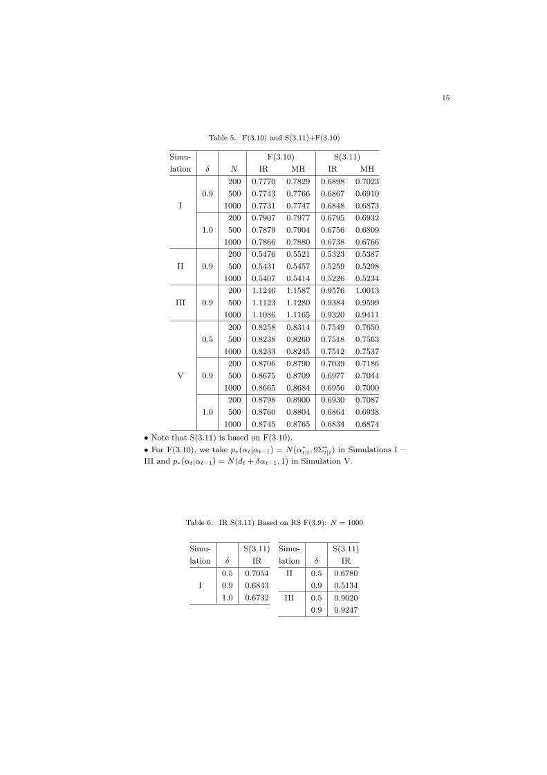
Table 5. F(3.10) and S(3.11)+F(3.10)
Simu- F(3.10) S(3.11)
lation δ N IR MH IR MH
200 0.7770 0.7829 0.6898 0.7023
0.9 500 0.7743 0.7766 0.6867 0.6910
I 1000 0.7731 0.7747 0.6848 0.6873
200 0.7907 0.7977 0.6795 0.6932
1.0 500 0.7879 0.7904 0.6756 0.6809
1000 0.7866 0.7880 0.6738 0.6766
200 0.5476 0.5521 0.5323 0.5387
II 0.9 500 0.5431 0.5457 0.5259 0.5298
1000 0.5407 0.5414 0.5226 0.5234
200 1.1246 1.1587 0.9576 1.0013
III 0.9 500 1.1123 1.1280 0.9384 0.9599
1000 1.1086 1.1165 0.9320 0.9411
200 0.8258 0.8314 0.7549 0.7650
0.5 500 0.8238 0.8260 0.7518 0.7563
1000 0.8233 0.8245 0.7512 0.7537
200 0.8706 0.8790 0.7039 0.7186
V 0.9 500 0.8675 0.8709 0.6977 0.7044
1000 0.8665 0.8684 0.6956 0.7000
200 0.8798 0.8900 0.6930 0.7087
1.0 500 0.8760 0.8804 0.6864 0.6938
1000 0.8745 0.8765 0.6834 0.6874
• Note that S(3.11) is based on F(3.10).
• For F(3.10), we take p∗(αt|αt−1) = N(α∗t|t, 9Σ∗
t|t) in Simulations I –
III and p∗(αt|αt−1) = N(dt + δαt−1, 1) in Simulation V.
Table 6. IR S(3.11) Based on RS F(3.9): N = 1000
Simu- S(3.11)
lation δ IR
0.5 0.7054
I 0.9 0.6843
1.0 0.6732
Simu- S(3.11)
lation δ IR
II 0.5 0.6780
0.9 0.5134
III 0.5 0.9020
0.9 0.9247

16
Table 7. IR S(3.11) Based on IR F(3.9): N = 1000
Simu- δ \ N ′ 1000 250 100 50 10
lation
0.5 0.7060 0.7059 0.7059 0.7059 0.7060
I 0.9 0.6851 0.6851 0.6853 0.6854 0.6869
1.0 0.6743 0.6744 0.6745 0.6748 0.6764
II 0.5 0.6795 0.6795 0.6796 0.6798 0.6813
0.9 0.5170 0.5173 0.5177 0.5198 0.5517
III 0.5 0.9024 0.9025 0.9027 0.9028 0.9045
0.9 0.9277 0.9305 0.9326 0.9393 0.9846
IV 4.3179 4.3392 4.4116 4.5086 4.9619
Table 8. Estimation of δ Using IR F(3.9): N = 1000
Simu- δ AVE SER 10% 25% 50% 75% 90%
Lation
0.5 0.481 0.129 0.30 0.41 0.50 0.57 0.63
I 0.9 0.881 0.059 0.80 0.85 0.89 0.92 0.94
1.0 0.983 0.033 0.94 0.97 0.99 1.00 1.01
II 0.5 0.313 0.202 0.00 0.16 0.32 0.45 0.58
0.9 0.670 0.201 0.44 0.54 0.67 0.81 0.98
III 0.5 0.503 0.022 0.49 0.50 0.50 0.51 0.52
0.9 0.902 0.019 0.88 0.89 0.90 0.91 0.92

17
than filtering. Moreover, as it is expected, RS shows the smallest RMSE in almost allthe cases. Taking an example of δ = 0.9 in Simulation I, N = 200 of RS is equal toN = 1000 of MH, which implies that MH needs 5 times more random draws than RSto keep the same precision, or equivalently the acceptance rate in RS is about 20% onaverage (note that this is a rough interpretation because RSME is not a linear functionof N). For δ = 0.9 of Simulation I, N = 500 of RS is almost equal to N = 1000 of IR,which implies that IR needs twice as many random draws as RS. Taking Simulation IV,N = 200 of RS is better than N = 1000 of IR. IR needs more than 5 times as manyrandom draws as RS. Simulation VI represents a multivariate non-Gaussian case, whereRS in S(3.11)+F(3.9) represents IR S(3.11) based on RS F(3.9). Thus, in SimulationVI, we utilize IR for smoothing because it is not easy to compute the supremum ofq3(αt+1, αt). The RMSEs are shown for both α1t and α2t in Simulation VI of Table 3.For both filtering and smoothing, RMSEs of RS are the smallest.
In Table 5, p∗(αt|αt−1) is introduced for filtering, but not for smoothing, wherep∗(αt|αt−1)p(αt−1|Yt−1) is used for the sampling density in Table 5 while p(αt|Yt−1) isused for sampling density in Table 3. For F(3.10) in Simulations I – III, p∗(αt|αt−1) =N(α∗
t|t, cΣ∗t|t) and c = 9 are taken. (α∗
t|t, Σ∗t|t) denotes the mean and variance estimated
by the extended Kalman filter, which is obtained by applying the linearized nonlinearmeasurement and transition equations directly to the standard Kalman filter formula(see, for example, Tanizaki (1996) and Tanizaki and Mariano (1996)). For F(3.10) inSimulation V, p∗(αt|αt−1) = N(dt + δαt−1, 1) is taken. Since it is difficult to computethe supremum of q2, RS is not shown in Table 5. We can compare F(3.9) in Table 3 withF(3.10) in Table 5 for filtering, and S(3.11)+F(3.9) in Table 3 with S(3.11)+F(3.10) inTable 5 for smoothing. For Simulation I, the RMSEs in Table 5 are very close to those inTable 3. For Simulations II and III, however, the RMSEs in Table 3 are slightly smallerthan those in Table 5 in almost all the cases. For Simulation V, Tables 3 and 5 arecompared. We consider the case where the data generating process is different from theestimated state space model. We often have this case in practice, because nobody knowsthe ture model. For F(3.10) of Simulation V in Table 5, p∗(αt|αt−1) = N(dt + δαt−1, 1)is taken. In other words, in Table 5 the sampling density is appropriately specifiedtaking into account the sudden shifts. It is expected for Simulation V that RS in Table3 should be close to IR and MH in Table 5, rather than those in Table 3. As a result, itis shown that for IR and MH we obtain a small RMSE if the plausible sampling densityp∗(αt|αt−1) is chosen, because the RMSEs of IR and MH in Table 3 are larger than thosein Table 5. Thus, two types of the sampling density p∗(αt|αt−1) are shown in Table 5,although we can consider the other kinds of the sampling density.
In Table 6, S(3.11)+F(3.9) is investigated, where we utilize RS for filtering and IRfor smoothing. Therefore, Table 6 should be compared with RS or IR in S(3.11)+F(3.9)of Table 3. Theoretically, the RMSEs in Table 6 should be between RS and IR inS(3.11)+F(3.9) of Table 3, since the most precise sampling method is used for filteringbut the second best one is utilized for smoothing. As a result, the RMSEs in Table 6are very close to those of RS in Table 3. It is sometimes difficult for the RS smoothersto compute the supremums based on (3.11), (3.12) and (3.14). In addition, RS takesa lot of time computationally although it is a very efficient random number generationmethod. The IR smoothers can be applied to almost all the nonlinear non-Gaussianstate space models, which give us much less computational burden than RS. Therefore,a combination of the RS filter based on (3.9) and the IR smoother might be a usefultool, judging from computation and efficiency.

18
In Table 7, we investigate how sensitive the approximation of p(αt+1|Yt) in equation(3.13) is, where N ′ = 10, 50, 100, 250, 1000 and N = 1000 are taken. IR is used for thesampling method. N ′ = 1000 in Table 7 is equivalent to N = 1000 of IR in Table 3. Wehave the result that N ′ = 1000 is very close to N ′ = 100, 250 in the RMSE criterion.Since for smoothing the order of computation is N×N ′, we can reduce the computationalburden by taking N ′ less than N , where we may take N ′ = 0.1N – 0.25N from Table 7.
In Table 8, we show an example to estimate the unknown parameter maximizingthe likelihood function (3.8), where IR is used for the sampling method. The likelihoodfunction is maximized by a simple grid search. AVE, SER, 10%, 25%, 50%, 75% and90% denote the arithmetic average, the standard error, 10th, 25th, 50th, 75th and 90thpercentiles from 1000 estimates of δ. For Simulations I and III, MLE shows a goodperformance because AVE and 50% are close to δ. However, for Simulation II, δ isunderestimated and SER is large.
Thus, in this section, we have shown some examples of RS, IR and MH for filteringand smoothing.
5. Summary
In this paper, we have shown the nonlinear non-Gaussian filtering and smotheringprocedures in general formulation, where RS, IR and MH are applied to generate randomdraws of αt given Ys. The existing simulation-based procedures are very computer-intensive, because conventionally they are based on the marginal density, i.e., p(αt|Yt)for filtering and p(αt|YT ) for smoothing. However, our proposal is based on the jointdensity, i.e., p(αt, αt−1|Yt) for filtering and p(αt+1, αt|YT ) or p(αt+1, αt, αt−1|YT ) forsmoothing. To reduce computational disadvantages, in this paper we have suggestedsampling from the joint densities.
It might be expected that RS gives us the most precise state estimates and that MHyields the worst of the three sampling techniques, which results are consistent with thesimulation results from the Monte Carlo studies. For RS, however, we need to computethe supremum in the acceptance probability. Especially, as for (3.10) – (3.12) and (3.14),we often have the case where the supremum does not exist or the case where it is difficultto compute the supremum. Therefore, for (3.10) – (3.12) and (3.14), it is better to utilizeIR, rather than RS and MH. Moreover, even though the supremum exists, computationaltime of RS depends on the acceptance probability. When the acceptance probability isclose to zero, it takes a lot of time computationally to obtain the random draws ofthe state variable αt. Both MH and IR can be applied to almost all the nonlinear non-Gaussian cases, which is one of the advantages over RS, although MH and IR are inferiorto RS in the sense of precision of the state estimates. Moreover, computational burdenof IR and MH does not depend on the acceptance probability. Accordingly, in the caseof IR and MH, (3.9) is computationally equivalent to (3.10) for filtering and similarly(3.11), (3.12) and (3.14) give us the same computational burden for smoothing.
It is possible to take different sampling methods between filtering and smoothing,i.e., for example, RS may be taken for filtering while IR is used for smoothing (seeRS in S(3.11) of Simulation VI of Table 3 and Table 6). Or at different time periodswe can adopt different sampling densities. That is, taking an example of filtering, thesampling density is taken as p∗(αt|αt−1)p(αt−1|Yt−1) if t = t′ and p(αt|Yt−1) otherwise.It might be useful to introduce p∗(αt|αt−1) when p(αt|Yt) is far from from p(αt|Yt−1).See Simulation V in Table 5 for this exercise. Thus, the proposed filters and smoothers
19
are very flexible. Taking the advantages of each sampling method, we can obtain theless computational and precise state estimates for both filtering and smoothing.
Moreover, we need to point out as follows. Smoothing is much more computer-intensive than filtering. That is, at each time period, the order of computation is N forfiltering and N ×N ′ for smoothing. Accordingly, smoothing is N ′ times more computer-intensive than filtering. In equation (3.13), we do not necessarily choose N ′ = N . Toreduce the computational disadvantage for smoothing, from the Monte Carlo studies(i.e., Table 7) we have obtained the result that we may take N ′ = 0.1N – 0.25N .
Finally, note as follows. For comparison with the procedure suggested in this paper,the smoother based on the two-filter formula, which is developed by Kitagawa (1996), isdiscussed in Appendix A. We have shown that using the sampling density the smootheris also rewritten in the same fashion. For Simulations I – III, the simulations studies areexamined. As a result, it is shown that the smoother based on the two-filter formulashows a good performance.
Appendix A: Fixed-Interval Smoother based on the Two-Filter Formula
Kitagawa (1996) discusses the Monte Carlo smoother based on the two-filter for-mula, where the same approach shown in this paper can be applied. Define Y +
t ≡yt, yt+1, · · · , yT , where we have YT = Yt−1 ∪Y +
t . The fixed-interval smoothing densityp(αt|YT ) is represented as:
p(αt|YT ) ∝ p(Y +t |αt)p(αt|Yt−1),(A.1)
where p(Y +t |αt) is recursively obtained as follows:
p(Y +t |αt) = py(yt|αt)
∫p(Y +
t+1|αt+1)pα(αt+1|αt)dαt+1,(A.2)
for t = T − 1, T − 2, · · · , 1. The initial condition is given by: p(Y +T |αT ) = py(yT |αT ).
First, we consider evaluating p(Y +t |αt) in the backward recursion. Let p∗(αt) be
the importance sampling density and α∗i,t be the i-th random draw of αt generated from
p∗(αt). From equation (A.2), the density p(Y +t |αt) evaluated at αt = α∗
i,t is rewrittenas:
p(Y +t |α∗
i,t) = py(yt|α∗i,t)
∫p(Y +
t+1|αt+1)pα(αt+1|α∗i,t)
p∗(αt+1)p∗(αt+1)dαt+1
≈ py(yt|α∗i,t)
1
N ′′
N ′′∑
j=1
p(Y +t+1|α
∗j,t+1)pα(α∗
j,t+1|α∗i,t)
p∗(α∗j,t+1)
,(A.3)
for t = T − 1, T − 2, · · · , 1. In the second line of the above equation, the integration isevaluated by α∗
j,t+1, j = 1, 2, · · · , N ′′, where N ′′ is not necessarily equal to N . Thus,
p(Y +t |α∗
i,t) is recursively obtained for t = T − 1, T − 2, · · · , 1. Note that the importancesampling density p∗(αt) may depend on the state variable at time t − 1, where thesampling density is given by p∗(αt|αt−1)
Next, given p(Y +t |α∗
i,t), we generate random draws of αt from p(αt|YT ). We canrewrite equation (A.1) as follows:
p(αt|YT ) ∝ q6(αt)p(αt|Yt−1),(A.4)
20
where q6(αt) ∝ p(Y +t |αt). In this case, we have to take the importance sampling density
as p∗(αt) = p(αt|Yt−1), i.e., α∗i,t = αi,t|t−1, where we need to evaluate p(αj,t+1|t|Yt) in
the denominator of equation (A.3). As shown in equation (3.13), however, evaluation ofp(αj,t+1|t|Yt) becomes N ′ times more computer-intensive. Therefore, it is not realisticto take the sampling density as p∗(αt) = p(αt|Yt−1).
Alternatively, as discussed in Section 3., we can consider generating random drawsfrom the joint density of αt and αt−1 given YT , which is represented by:
p(αt, αt−1|YT ) ∝ q7(αt, αt−1)p∗(αt)p(αt−1|Yt−1),(A.5)
where q7(αt, αt−1) ∝p(Y +
t |αt)pα(αt|αt−1)
p∗(αt).
As shown above, we can evaluate p(Y +t |αt) at αt = α∗
i,t. However, an explicit func-
tional form of p(Y +t |αt) is not obtained and it is not possible to compute the supremum
of q6(αt) and q7(αt, αt−1). Therefore, RS cannot be applied to this smoother. Thus, wemay apply IR and MH to the Monte Carlo smoother based on the two-filter formula.
Taking an example of the IR smoother based on (A.5), a random number of αt
from p(αt|YT ) is generated as follows. Define the probability weight ω(α∗i,t, αi,t−1|t−1)
which satisfies ω(α∗i,t, αi,t−1|t−1) ∝ q7(α
∗i,t, αi,t−1|t−1) and
∑Ni=1 ω(α∗
i,t, αi,t−1|t−1) =1. Thus, from equation (A.1), the j-th smoothing random draw αj,t|T is resampledfrom α∗
1,t, α∗2,t, · · ·, α∗
N,t with the corresponding probability weights ω(α∗1,t, α1,t−1|t−1),
ω(α∗2,t, α2,t−1|t−1), · · ·, ω(α∗
N,t, αN,t−1|t−1). Computing time of the IR smoother basedon (A.5) is the order of N × N ′′, which is equal to IR in Table 2, while that of the IRsmoother with (A.4) is N ×N ′ ×N ′′. Thus, for reduction of computational burden, useof (A.5) is superior to that of (A.4).
One of the computational techniques is shown as follows. The dimension of Y +t
increases as t is small. That is, p(Y +t |α∗
i,t) for all i decreases as t goes to the initial timeperiod. Therefore, practically we have some computational difficulties such as underflowerrors. To avoid the computational difficulties, we can modify equation (A.3) as follows:
st(α∗i,t) ∝ py(yt|α
∗i,t)
N ′′∑
j=1
st+1(α∗j,t+1)pα(α∗
j,t+1|α∗i,t)
p∗(α∗j,t+1)
,
where st(α∗i,t) ∝ p(Y +
t |α∗i,t). For instance, st(αt) may be restricted to
∑Ni=1 st(α
∗i,t) =
1. We need to compute st(α∗i,t) whenever we update from t + 1 to t. Note that the
proportional relation q7(α∗i,t, αi,t−1|t−1) ∝
st(α∗i,t)pα(α∗
i,t|αi,t−1|t−1)
p∗(α∗i,t)
still holds.
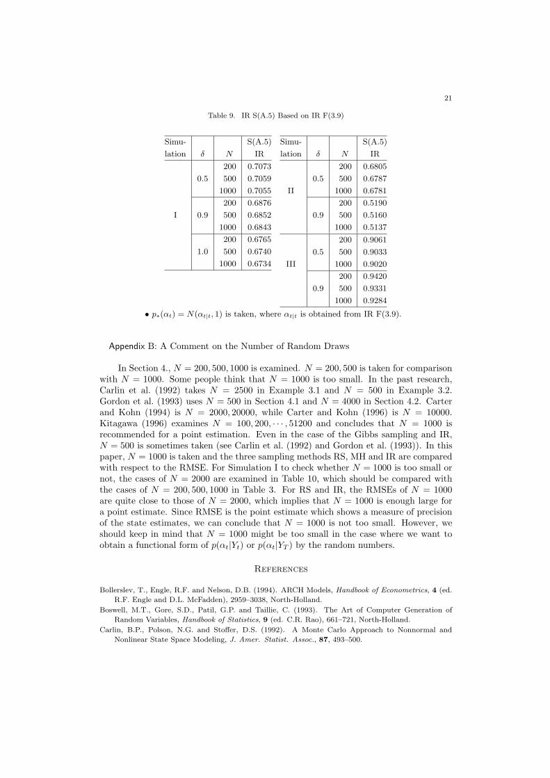
Thus, the fixed-interval smoother based on the two-filter formula, proposed by Kita-gawa (1996), can be also discussed in the same context. In Table 9, the smoother basedon the two-filter formula is examined for Simulations I – III. We take p∗(αt) = N(αt|t, 1),where αt|t represents the filtering estimate obtained from IR F(3.9). After implementingIR F(3.9), we perform IR S(A.5). Each value in Table 9 is compared with that in IRS(3.11) of Table 3. As a result, IR S(A.5) performs much better than IR S(3.11) inalmost all the cases.
21
Table 9. IR S(A.5) Based on IR F(3.9)
Simu- S(A.5)
lation δ N IR
200 0.7073
0.5 500 0.7059
1000 0.7055
200 0.6876
I 0.9 500 0.6852
1000 0.6843
200 0.6765
1.0 500 0.6740
1000 0.6734
Simu- S(A.5)
lation δ N IR
200 0.6805
0.5 500 0.6787
II 1000 0.6781
200 0.5190
0.9 500 0.5160
1000 0.5137
200 0.9061
0.5 500 0.9033
III 1000 0.9020
200 0.9420
0.9 500 0.9331
1000 0.9284
• p∗(αt) = N(αt|t, 1) is taken, where αt|t is obtained from IR F(3.9).
Appendix B: A Comment on the Number of Random Draws
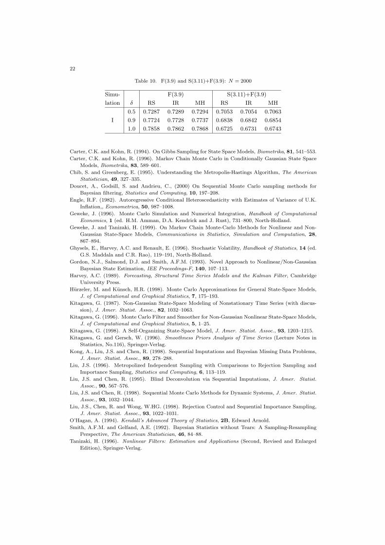
In Section 4., N = 200, 500, 1000 is examined. N = 200, 500 is taken for comparisonwith N = 1000. Some people think that N = 1000 is too small. In the past research,Carlin et al. (1992) takes N = 2500 in Example 3.1 and N = 500 in Example 3.2.Gordon et al. (1993) uses N = 500 in Section 4.1 and N = 4000 in Section 4.2. Carterand Kohn (1994) is N = 2000, 20000, while Carter and Kohn (1996) is N = 10000.Kitagawa (1996) examines N = 100, 200, · · · , 51200 and concludes that N = 1000 isrecommended for a point estimation. Even in the case of the Gibbs sampling and IR,N = 500 is sometimes taken (see Carlin et al. (1992) and Gordon et al. (1993)). In thispaper, N = 1000 is taken and the three sampling methods RS, MH and IR are comparedwith respect to the RMSE. For Simulation I to check whether N = 1000 is too small ornot, the cases of N = 2000 are examined in Table 10, which should be compared withthe cases of N = 200, 500, 1000 in Table 3. For RS and IR, the RMSEs of N = 1000are quite close to those of N = 2000, which implies that N = 1000 is enough large fora point estimate. Since RMSE is the point estimate which shows a measure of precisionof the state estimates, we can conclude that N = 1000 is not too small. However, weshould keep in mind that N = 1000 might be too small in the case where we want toobtain a functional form of p(αt|Yt) or p(αt|YT ) by the random numbers.
References
Bollerslev, T., Engle, R.F. and Nelson, D.B. (1994). ARCH Models, Handbook of Econometrics, 4 (ed.
R.F. Engle and D.L. McFadden), 2959–3038, North-Holland.
Boswell, M.T., Gore, S.D., Patil, G.P. and Taillie, C. (1993). The Art of Computer Generation of
Random Variables, Handbook of Statistics, 9 (ed. C.R. Rao), 661–721, North-Holland.
Carlin, B.P., Polson, N.G. and Stoffer, D.S. (1992). A Monte Carlo Approach to Nonnormal and
Nonlinear State Space Modeling, J. Amer. Statist. Assoc., 87, 493–500.
22
Table 10. F(3.9) and S(3.11)+F(3.9): N = 2000
Simu- F(3.9) S(3.11)+F(3.9)
lation δ RS IR MH RS IR MH
0.5 0.7287 0.7289 0.7294 0.7053 0.7054 0.7063
I 0.9 0.7724 0.7728 0.7737 0.6838 0.6842 0.6854
1.0 0.7858 0.7862 0.7868 0.6725 0.6731 0.6743
Carter, C.K. and Kohn, R. (1994). On Gibbs Sampling for State Space Models, Biometrika, 81, 541–553.
Carter, C.K. and Kohn, R. (1996). Markov Chain Monte Carlo in Conditionally Gaussian State Space
Models, Biometrika, 83, 589–601.
Chib, S. and Greenberg, E. (1995). Understanding the Metropolis-Hastings Algorithm, The American
Statistician, 49, 327–335.
Doucet, A., Godsill, S. and Andrieu, C., (2000) On Sequential Monte Carlo sampling methods for
Bayesian filtering, Statistics and Computing, 10, 197–208.
Engle, R.F. (1982). Autoregressive Conditional Heteroscedasticity with Estimates of Variance of U.K.
Inflation,, Econometrica, 50, 987–1008.
Geweke, J. (1996). Monte Carlo Simulation and Numerical Integration, Handbook of Computational
Economics, 1 (ed. H.M. Amman, D.A. Kendrick and J. Rust), 731–800, North-Holland.
Geweke, J. and Tanizaki, H. (1999). On Markov Chain Monte-Carlo Methods for Nonlinear and Non-
Gaussian State-Space Models, Communications in Statistics, Simulation and Computation, 28,
867–894.
Ghysels, E., Harvey, A.C. and Renault, E. (1996). Stochastic Volatility, Handbook of Statistics, 14 (ed.
G.S. Maddala and C.R. Rao), 119–191, North-Holland.
Gordon, N.J., Salmond, D.J. and Smith, A.F.M. (1993). Novel Approach to Nonlinear/Non-Gaussian
Bayesian State Estimation, IEE Proceedings-F, 140, 107–113.
Harvey, A.C. (1989). Forecasting, Structural Time Series Models and the Kalman Filter, Cambridge
University Press.
Hurzeler, M. and Kunsch, H.R. (1998). Monte Carlo Approximations for General State-Space Models,
J. of Computational and Graphical Statistics, 7, 175–193.
Kitagawa, G. (1987). Non-Gaussian State-Space Modeling of Nonstationary Time Series (with discus-
sion), J. Amer. Statist. Assoc., 82, 1032–1063.
Kitagawa, G. (1996). Monte Carlo Filter and Smoother for Non-Gaussian Nonlinear State-Space Models,
J. of Computational and Graphical Statistics, 5, 1–25.
Kitagawa, G. (1998). A Self-Organizing State-Space Model, J. Amer. Statist. Assoc., 93, 1203–1215.
Kitagawa, G. and Gersch, W. (1996). Smoothness Priors Analysis of Time Series (Lecture Notes in
Statistics, No.116), Springer-Verlag.
Kong, A., Liu, J.S. and Chen, R. (1998). Sequential Imputations and Bayesian Missing Data Problems,
J. Amer. Statist. Assoc., 89, 278–288.
Liu, J.S. (1996). Metropolized Independent Sampling with Comparisons to Rejection Sampling and
Importance Sampling, Statistics and Computing, 6, 113–119.
Liu, J.S. and Chen, R. (1995). Blind Deconvolution via Sequential Imputations, J. Amer. Statist.
Assoc., 90, 567–576.
Liu, J.S. and Chen, R. (1998). Sequential Monte Carlo Methods for Dynamic Systems, J. Amer. Statist.
Assoc., 93, 1032–1044.
Liu, J.S., Chen, R. and Wong, W.HG. (1998). Rejection Control and Sequential Importance Sampling,
J. Amer. Statist. Assoc., 93, 1022–1031.
O’Hagan, A. (1994). Kendall’s Advanced Theory of Statistics, 2B, Edward Arnold.
Smith, A.F.M. and Gelfand, A.E. (1992). Bayesian Statistics without Tears: A Sampling-Resampling
Perspective, The American Statistician, 46, 84–88.
Tanizaki, H. (1996). Nonlinear Filters: Estimation and Applications (Second, Revised and Enlarged
Edition), Springer-Verlag.

23
Tanizaki, H. (1999). On the Nonlinear and Nonnormal Filter Using Rejection Sampling, IEEE Trans.
Automat. Control, 44, 314–319.
Tanizaki, H. (2000). Nonlinear and Non-Gaussian State-Space Modeling with Monte Carlo Techniques:
A Survey and Comparative Study, Handbook of Statistics (Stochastic Processes: Modeling and
Simulation) (ed. C.R. Rao and D.N. Shanbhag), North-Holland, forthcoming.
Tanizaki, H. and Mariano, R.S. (1996). Nonlinear Filters Based on Taylor Series Expansions, Commu-
nications in Statistics, Theory and Methods, 25, 1261–1282.
Tanizaki, H. and Mariano, R.S. (1998). Nonlinear and Non-Gaussian State-Space Modeling with Monte
Carlo Simulations, J. of Econometrics, 83, 263–290.