nonexpected utility preferences in a temporal framework with...

JOURNAL OF ECONOMIC THEORY 9. 54-81 (1990)

Nonexpected Utility Preferences in a Temporal Framework with an Application

to Consumption-Savings Behaviour*

Soo HONG CHEW

Department of’ Economics, The Johns Hopkins Uniclersiry. Baltimore, Maryland 21218

AND

LARRY G. EPSTEIN

Department (v’ Economics, University of Toronfo, Toronto. Onrario, Canada M5S IA1

Received June 7, 1988; revised January 12, 1989

This paper investigates the role of non-expected utility preferences in a multi- period consumption/savings framework. Three objectives are achieved: First, it is shown that behaviour can be intertemporally consistent even if the preference ordering is not. Second, non-expected utility preference orderings are shown to be useful for disentangling the elasticity of intertemporal substitution from the degree of risk aversion. Finally, some discrimination between the non-expected utility theories that have appeared in the atemporal literature is achieved by means of axioms which arise naturally from the multiperiod framework. Journal of‘ Economic Literature Classification Numbers: 022, 026. ( 1990 Academic Press. Inc.

1. INTRODUCTION

Expected utility theory continues to dominate the economics of uncertainty. But recently there has been “a growing tendency to view expected utility maximization less and less as the only form of “rational” behaviour under uncertainty and more and more as a refutable scientific hypothesis, to be judged against competing models on the basis of the data” [25, p. 11. Evidence against the empirical validity of expected utility theory has

* The financial support of the National Science Foundation is gratefully acknowledged. We are also grateful to Mark Machina and a referee for suggestions which substantially improved the exposition.

54 0022-053 l/90 $3.00 Copyright 0 1990 by Academic Press, Inc All right, or reproduction m any form reserved

NON-EXPECTED UTILITY 55

accumulated in the behavioural experimentation literature originating with the Allais paradox. Several alternative theories, which are nonlinear in probabilities, have been proposed. It has been shown that they can account for many of these behavioural paradoxes while still retaining normatively appealing properties such as consistency with stochastic dominance and risk aversion. (See [26] for a survey.) These theories and the surrounding applications have been formulated largely in atemporal frameworks, where decisions subject to uncertainty are made at one point in time and/or all consumption takes place at one point in time.’ In contrast, in the real time framework of this paper uncertain consumption sequences are the ultimate source of utility and choices are made sequentially subject to changing information about the state of the world. It is only in such a framework that one can investigate the usefulness of nonlinear theories of preference for explaining consumption and savings behaviour. This paper attempts such an investigation.

Three questions form the heart of this paper:

(a) Can behaviour which is dictated by a non-expected utility preference ordering be intertemporally consistent?

(b) Can we discriminate amongst the newly proposed theories on the basis of theoretical considerations that arise in a temporal setting?

(c) Are nonlinear theories “useful” for modelling consumption and savings behaviour?

The remainder of this introduction will elaborate on these questions and briefly outline the answers developed below.

With regard to question (c) we are motivated by the desire to specify intertemporal utility functionals which permit properties of ordinal preferences (the elasticity of intertemporal substitution) and risk preferences (the degree of risk aversion) to be disentangled. In the common expected utility specification with an intertemporally additive von NeumannMorgenstern utility index, both of the above aspects of preferences are embodied in the curvature of the within-period utility function. Selden [36] and [37], as discussed further below, proposes a generalization of the standard specification which eliminates this inflexibility. The issue of the separation of “time” and “risk” preferences has arisen in the empirical macro literature which attempts to explain the time series behaviour of consumption and asset returns. The standard expected utility models have not performed well empirically [ 161 and it has been conjectured [ 14, 15,441 that this poor performance may be due to the inflexibility of the preference specification which employs a single

I This description also applies to [ 131 and [IS] where dynamic choices do not lead to actual consumption until an elementary consequence is encountered at a terminal node.

56 CHEW AND EPSTEIN

parameter to measure both risk aversion and substitutability. The limited flexibility of the standard expected utility specification has also been noted in the stochastic growth literature [S, p. 1013, p. 10221 and in the theoretical asset pricing literature [24, p. 14411.

Our analysis of preference is axiomatic. One key axiom considered below is recursivity or the intertemporal consistency of preference. Another central axiom, called ordinal dominance, relates the ranking of random consumption sequences to the ranking of deterministic sequences. Roughly, it states that if two random requences, C and C’, are such that in every state of the world, the deterministic consumption stream provided in C is weakly preferred to that provided in C’, then C should be weakly preferred to C’. It is well known [32, p. 821 that there is a close link between intertemporal consistency and the independence axiom (IA) of expected utility theory. Below (see the discussion following Theorem 3.1) we also draw a parallel between ordinal dominance and the reduction of compound lotteries axiom (ROCLA). Since IA and ROCLA constitute the cornerstones of expected utility theory, it is not surprising that we show below that recursivity and ordinal dominance (and other less critical axioms) imply an intertemporal expected utility function. Given the inflexibility of the latter noted above we are forced to choose which of recursivity and ordinal dominance to weaken. We are not aware of any empirical evidence which bears directly on this choice and we feel that both of the possible routes are worth exploring. In this paper we pursue the route of weakening recursivity. We note that in light of the link between recursivity and the independence axiom, this route is consistent with the thrust of much of the atemporal non-expected utility literature (see [25], in particular) which interprets experimental violations of the expected utility model as violations of independence. That literature attempts to explain experimental results by means of generalized theories which weaken independence. The implied remedy for the present temporal context is to weaken recursivity.

The alternative route of maintaining recursivity has been pursued by Epstein and Zin [ 10 J, building upon earlier work by Kreps and Porteus [21]. The separation of “time” and “risk” preferences is also possible within the Selden [36, 371 specification. These published analyses are formulated in a two-period setting, but a multi-period extension is possible [38]. This multi-period specification violates both recursivity and ordinal dominance. Moreover, since it is based on expected utility for single period gambles it is incompatible with the experimental evidence against expected utility theory. In contrast, the specifications developed in this paper are compatible with that evidence.

Since the recursivity axiom is deleted, a consumption plan formulated at t =0 may not be pursued in subsequent periods. The resulting inconsistency of plans is not an issue if precommitment is possible and this


scenario is considered below. But what are reasonable assumptions about

consumer behaviour when precommitment is not possible? Similar questions have arisen in the literatures on planning with changing tastes [40, 29, 283 and growth with imperfect intergenerational altruism [22]. Two hypotheses that have been explored are (i) naive choice, where the consumer ignores future inconsistencies, and (ii) sophisticated choice, where inconsistencies are resolved by taking future consumption levels as a constraint when choosing current consumption. The latter approach is the more prevalent one in the cited literatures and is adopted here.’ Formally, the decision problem is modelled as a noncooperative game between decision makers at different times and a (stationary) perfect Nash equilibrium is used to describe behaviour. 3 The equilibrium represents a time-consistent form of behmiour, even though preferences are not intertemporally consistent and thus the first question posed above is answered.

To demonstrate the “usefulness” of nonlinear theories (question (c)), we apply the preference orderings which satisfy our axioms to analyse behaviour in a standard setting where the random returns to savings are identically and independently distributed over time. The resulting model is shown to be tractable in that it is amenable to comparative dynamics analysis. Of particular interest is the effect on behaviour of increased risk aversion. For the reasons given above, such comparative risk aversion analysis cannot be performed satisfactorily in the expected utility framework.

Finally, consider question (b). The (transitive) nonlinear preference theories which have been axiomatized in an atemporal framework include the betweenness-conforming theories [ 12, 91, the subclass of weighted utility theories [2, 61, and anticipated or rank-dependent utility theories [30, 35, 2, 431. Only the latter class is compatible with the axiomatic structure of this paper, at least if the common intersection of these theories, expected utility theory, is excluded. There are two important differences between existing atemporal axiomatic analyses and our own: First, we are unable to determine completely the functional form structure which corresponds to our axioms. On the other hand, our central axioms depend critically on the multi-period framework and they arise naturally from it.

The paper proceeds as follows: Some preliminary notions and important examples are presented in Section 2. Our formal analysis of preferences is

’ For an alternative approach see [41]. which proposes an “organizational” view of the consumer as made up of a planner and many selfish doers (one for each period). In contrast. there is the view of Stigler and Becker 1391 that many apparent changing taste phenomena can be modelled in a constant taste framework where inconsistencies do not arise. The usefulness of their approach to our stochastic setting remains to be explored.

’ Karni and Safra [ 181 adopt a similar game-theoretic approach to the description of behaviour in auctions given non-expected utility preferences. But see footnote 1.

58 CHEW AND EPSTEIN

undertaken in Section 3. Behaviour in the context of a simple but standard planning environment is analysed in Section 4 under the assumption that plans are not binding and in Section 5 under the assumption that commitment is possible. Some concluding remarks are offered in Section 6. Proofs are collected in an appendix.

2. PRELIMINARIES

Fix 0 < 6 < 1. Define 1: + (6) = { y = (c, , . . . . cI, . . . ): c, > 0 for all t and CS’c,<co) and endow l’++(6) with the product topology. The basic choice space is P = (0, cc ) x M(I: + (6)), where for any topological space X, M(X) denotes the space of Bore1 probability measures on X, endowed with the weak convergence topology. For a typical element (c,, p) E P, called a consumption program or path, c,, represents the certain current level of consumption and the probability measure p represents the uncertain future. Note that any y E 1: + (6) can be identified in the usual fashion with the measure assigning unit mass to {JJ}. Thus we often write

(co, v) E P and we interpret (c,, .v) as a deterministic consumption program.

Preference orderings 2 on P are assumed to be reflexive and transitive but possibly incomplete. Completeness is not imposed because of the well- known possibilities of non-comparability which arise in infinite horizon settings for consumption programs in which consumption is unbounded above and/or not bounded away from zero.

A major thrust of this paper is the analysis of increased risk aversion. Thus it is necessary to provide a precise definition for “more risk averse than”:

DEFINITION 2.1. Let k* and 2 be preference orderings on P. Say that k* is more risk auerse than 2 if for all (c,, p) E P and y El: +(6),

(co, .v) 2 (C”? PI =a (CO? .v) 2* (COYP).

Consider a choice between the nonstochastic path (c,, y) and the (generally) stochastic path (c,, p). If one agent rejects the stochastic alternative, then so should the more risk averse agent. Of course two preference orderings which are comparable in this sense must rank deterministic consumption paths identically.

To conclude this section we present three examples of preference orderings. They will clarify the above definition and should also facilitate understanding of the axioms in the next section.

The first example is the standard time-separable expected utility

NON-EXPECTED UTILITY

specification where 2 is represented numerically u,,

59

by the utility functional

(CO? P) E p. (2.1)

Here 0 < /J < 1, f is increasing and concave on (0, co), and E, denotes the expected value according to the measure p.4 Any two distinct expected utility specifications U, and U,$ are not comparable according to Delini- tion 2.1, though if f * is more concave than f then U,tJf will show greater aversion to risks that are confined to consumption in one period. But then intertemporal substitutability is also changed in going from f to f*. For example, if the common homogeneous specification, f(c) = c’ “/( 1 - a), 0 < c( # 1, is adopted, then the “relative risk aversion parameter” a is also the reciprocal of the elasticity of substitution. Thus comparative statics analyses corresponding to changes in c( do not have a clear interpretation.

For the second example, consider first the utility functional I’, due to Yaari [43] and defined on D(R), the set of cumulative distribution functions (c.d.f.‘s) on the real line, by

where g: [IO, 1) + [0, l] is continuous and strictly increasing, g(0) = 0, and g( 1) = 1. This is a member of the rank-dependent utility class referred to in the introduction. The nature of Vy is clarified by considering c.d.f.‘s corresponding to binary gambles with outcomes z, and 22, -71 < z2. Then the associated utility according to V,. is

v,= dP, I:, + (1 - g(p, lb-2, (2.3)

where p, is the probability of the outcome z, If g(p) >p on [0, l] we see that (2.3) is an “expected value” but with probabilities transformed in such a way that the inferior outcome is given greater weight. This transformation leads to a certainty equivalent for the gamble which is less than its

expected value and thus implies a form a risk aversion, (See [2, 42, 51 for analyses of risk aversion for rank-dependent utility functionals.)

The Yaari functional (2.2) can be applied to define the intertemporal utility functional

(2.4)

4 In (2.1) and similar equations below. the equality is intended only on that subset of P where the right side is well defined as an extended real number. Thus the domain of U, is a proper subset of P and the corresponding ordering 2 is incomplete. Often in the literature 2 is extended by means of the overtaking criterion, but that extension is not considered here.

60 CHEW AND EPSTEIN

where (?,, F,, . ..) is any random variable sequence with probability measure p, F, = cO, and where for any extended real-valued random variable .f, F.? denotes its c.d.f. If g(p) -p then (2.4) reduces to the standard specification (2.1). But in the broader class with nonlinear g, greater risk aversion can be achieved by suitably modifying the probability transformation function. If R* and 2 are two orderings defined via (2.2) and (2.4) corresponding to g* and g respectively, then k* is more risk averse than 2 in the sense of Definition 2.1 if and only if g*(p) 3 g(p) on [0, 11.

These two examples reflect the general structure of intertemporal utility functionals considered in this paper. Informally, that structure corresponds to a two-stage algorithm used by the consumer to evaluate any given consumption program: first, the implied probability distribution is computed for the “present discounted utility”: and second, this distribution is evaluated by a univariate preference functional. More precisely,

(2.5)

where Y is a functional defined on D(R), increasing in the sense of first degree stochastic dominance and where the argument of V is defined analogously to (2.4). (In (2.1), V is the expected value functional while in the second example, V is the Yaari functional (2.2)) Given such a specification, the degree of risk aversion, at least for comparative purposes, is encoded in V( .), and thus is disentagled from intertemporal substitutability which is encoded in f( ).

Our approach to (2.5) is axiomatic. Moreover, our axioms will restrict the admissible Vs. In particular they will rule out the choice of

V(F)=/ w(z)dF(z), FE D(R), (2.6)

where w is increasing and (strictly) concave. In conjunction with (2.5) this leads to the expected value of w(x,” plf(c”,)), rather than (2.1). Adoption of such a concave transformation of the von Neumann-Morgenstern utility index is suggested by Kihlstrom and Mirman’s [19] approach to comparative risk aversion analysis in a multicommodity expected utility framework. But if w is not linear, then (2.5)-(2.6) violate one of our axioms (stationarity) and so is excluded here. A stronger (but related) argument against the adoption of the Kihlstrom and Mirman approach to comparative risk aversion analysis in multiperiod settings is described in [lo].

The final example mentioned here is due to Selden and Stux [38],

~.s(cot PI = t U(?,), (2.7) 0


where

P, = u-‘(E,u(T,))

and the expected value is computed with respect to the probability distribution for tth period consumption induced by p. Here U, is a discounted sum of within period utilities where the latter depend on the certainty equivalents ?,. Intertemporal substitutability is encoded in ,f and risk preferences in u. Increased concavity of u implies greater risk aversion in the sense of Definition 2.1. But the specification (2.7) will be ruled out by our axioms; in particular, note that it is not a special case of (2.5) unless o is linear and U, reduces to an expected utility functional.

3. PREFERENCE ORDERINGS

Consider the following axioms for the preference ordering 2 defined on P=(O, ~m)xM(l:+(6)):

Cm-taint>> Additivity. There exist a strictly concave and increasing function f: (0, r;o ) + ( - rx, w ) and 0 < fi < 1 such that the extended real-valued function U,

‘4.V %

I= c /MC,)> (3.1)

i) where xc B’f(c,) exists in an extended real valued sense, satisfies u( y’) 3 U(Y) o y’ 2 J’.’ defined on that subset of I’+ + (6

The additive functional form (3.1) dominates the capital theory literature including stochastic analyses where u is interpreted as a von Neumann- Morgenstern utility index. The above axiom requires that 2 agree with the additive ordering on deterministic paths. There exist numerous axiomatizations of additive orderings of deterministic programs [20, 311. Since we wish to focus on uncertainty and attitudes towards it, we have chosen simply to maintain certainty additivity. Of course, the strict concavity off is equivalent to the strict quasiconcavity of U.

For any p~M(1’++(6)), denote by Aop~M(1!,+(6)) the measure obtained from p by scaling all outcomes by the factor A; that is, ;10 p(Q) E p(AK’Q) for all measurable sets Q.

’ By u( v’) > U(J) we mean that both numbers lie in R* = [-IX), a] and are ordered there in the usual way. In particular. it is not true that + I;C = f z. This convention is adopted for all extended real-valued functions.

62 CHEW AND EPSTEIN

Homotheticity. For all i > 0 and (cb, p’), (c,, p) E P,

(c-b, p’) 2 (co, p) - (kb, 2 il p’) 2 (kl, 2 17 PI.

It is now immediate that the function f from (3.1) must have the form

Jc) = log c ,

i

e’- “/(l -a), O<cr#l cl= 1.

(3.2)

The specification (3.1) and (3.2) is a commonly considered special case for an intertemporal von Neumann-Morgenstern index ([34,23], for example). Thus homotheticity is natural in this initial attempt at an investigation of non-expected utility theories. Moreover, the resulting CES specification for intertemporal utility u is sufficiently flexible to permit the issue of the separation of ordinal and risk preferences to be addressed.

The next two axioms are central.

Ordinal Dominance. For every (cb, p’) and (c,, p) in P which are comparable according to 2, if p’1.r E j:+(6): (cb, I,) 2 j} 3 p{yEli++(6): (co. +r)kj) for all YEI:+ (6) (and if the inequality is strict for some j), then (cb, p’) 2 (>) (co, p).

The essence of the axiom is most easily grasped if it is restricted to consumption programs for which

p’( Y) = p( Y) = 11 Y- {yd++(6): -oO<U(JJ)<oD).

In that case, (CL, p’) and (c,, p) each induce a probability distribution for real-valued intertemporal utility as measured by U. Ordinal dominance requires that (cb, p’) be weakly (strictly) preferred to (c,, p) if (the two programs are comparable and) the distribution of utility induced by the former (strictly) dominates the distribution induced by the latter according to first degree stochastic dominance. In the stated axiom, a similar link between 2 and its certainty restriction is imposed on the entire program space P. (See the introduction for further interpretation of ordinal dominance.)

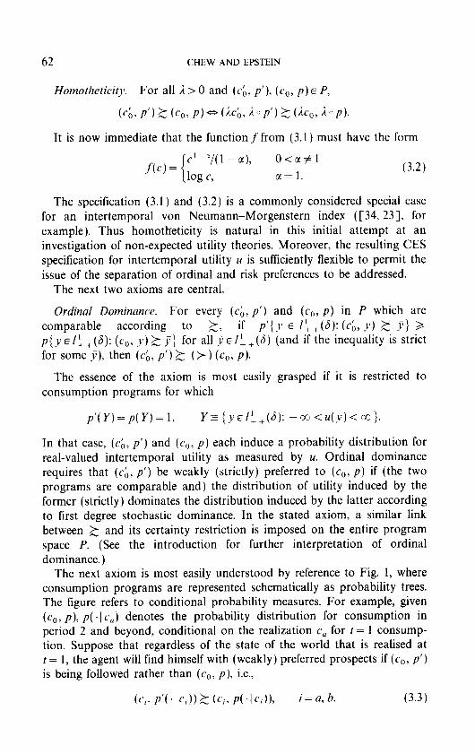
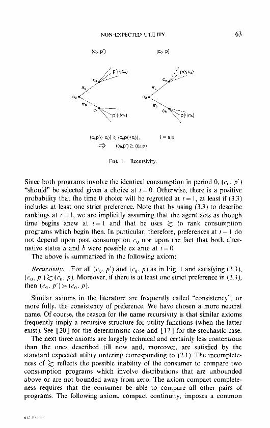
The next axiom is most easily understood by reference to Fig. 1, where consumption programs are represented schematically as probability trees. The figure refers to conditional probability measures. For example, given (c,, p), p( .I c,) denotes the probability distribution for consumption in period 2 and beyond, conditional on the realization c, for t = 1 consumption. Suppose that regardless of the state of the world that is realised at t = 1, the agent will find himself with (weakly) preferred prospects if (c,, p’) is being followed rather than (c,, p), i.e.,

tct, P’(‘Ici))k tci3 P(.lcr))3 i = a, b. (3.3)


(CO! P’) (co, P)

P’(.lCa) P(.lC=)

cs CZ3

TTa 7Ta

CO -:c. < CO

Bb TTb Cb Cb

P’(./Cb) P(.lCd

(C~,P’(+z)) z (GsP(4G)),

=> (Co,P’) 2 (Co,P)

i = a,b

FIG. 1. Recursivity.

Since both programs involve the identical consumption in period 0, (c,, p’) “should” be selected given a choice at t =O. Otherwise, there is a positive probability that the time 0 choice will be regretted at t = 1, at least if (3.3) includes at least one strict preference. Note that by using (3.3) to describe rankings at t = 1, we are implicitly assuming that the agent acts as though time begins anew at t = 1 and that he uses 2 to rank consumption programs which begin then. In particular, therefore, preferences at t = 1 do not depend upon past consumption c0 nor upon the fact that both alternative states a and b were possible ex ante at t = 0.

The above is summarized in the following axiom:

Recursiuitv. For all (c,, p’) and (c,, p) as in Fig. 1 and satisfying (3.3), (c,, p’) 2 (c,, p). Moreover, if there is at least one strict preference in (3.3), then (co, P’) > (co, PI.

Similar axioms in the literature are frequently called “consistency”, or more fully, the consistency of preference. We have chosen a more neutral name. Of course, the reason for the name recursivity is that similar axioms frequently imply a recursive structure for utility functions (when the latter exist). See [20] for the deterministic case and [ 171 for the stochastic case.

The next three axioms are largely technical and certainly less contentious than the ones described till now and, moreover, are satisfied by the standard expected utility ordering corresponding to (2.1). The incomplete- ness of 2 reflects the possible inability of the consumer to compare two consumption programs which involve distributions that are unbounded above or are not bounded away from zero. The axiom compact completeness requires that the consumer be able to compare all other pairs of programs. The following axiom, compact continuity, imposes a common

64 CHEW AND EPSTEIN

form of continuity while the final one, extendability, guarantees that the preference for a distribution cannot be “driven” by the tails. The latter would be irrelevant and the others standard if we restricted ourselves to suitably bounded probability measures in defining the outcome space. But such a domain is not sufficiently broad to contain the consumption programs that are optimal in the optimization problems of Sections 4 and 5. Thus the added complexity here is necessary for the later behavioural analysis.

The formulation of these axioms requires the following additional notation: For each 0 < I< L < w and p E M(I’+ +(6)), P,,~ denotes the truncation ofp onto [I, L]” defined as follows: Let 7~: 1: +(6)--f [C, L]” be defined by

c

(ny),- l’

1

16c,<L

c, d I

L c, 3 L.

Define p,,JQ)=p(z~‘(Q)) for all measurable sets Qc/:+(S)). Then P,,~ E M( [I, L]‘“), the set of probability measures with support in [I, L] X.

Compact Completeness. 2 is complete on (0, 00 ) x M( [I, L J “) for each O<I<L<oo.

Compact Continuity. For any 0 < 1 <L < W, 2 is continuous when restricted to (0, cc ) x M( [C, L] z ).

Extendability. For all (cb, p’) and (c,,, p) in P, if (cb, p’)> (c,, p), then 3O<I,<L,<cc; such that (~b,p;,~)>(c~,p,,,.) for all O<f<I, and L,<L<w.

Consider briefly the axioms specified to this point in the context of the examples defined in the preceding section. (Henceforth, let f in (2.1) (2.4), and (2.7) be defined by (3.2).) It is readily verified that the Yaari-based specification ((2.2), (2.4)) satisfies all of these axioms with the possible exception of recursivity. Note that ordinal dominance is a consequence of the general structure (2.5). Recursivity is satisfied if and only if the probability transformation function g is linear, in which case the expected utility specification (2.1) is obtained. In fact, the axioms stated thus far imply an expected utility specification as described in the first theorem of this section.

THEOREM 3.1. Let 2 satisfy the axioms certainty additivity, homotheticity, ordinal dominance, recursivity, compact completeness, compuct continuity. and extendability. Then ,for all consumption programs in P.

u,tc;,, p’) 2 ci,(c,, p) =s (cb, p’f 2 (co, p), (3.4)


hrhere U, is defined by (2.1) and (3.2). Conversely, the ordering represented by this expected utility specification satisfies all of the above axioms.

It can be shown that equivalence in (3.4) holds on P{, the subset of P defined in (4.2) below, which consists of all consumption programs which are intermediate in preference between some pair of deterministic and constant programs. On that set, at least, Theorem 3.1 shows that the stated axioms characterize the homothetic expected utility specification. The fact that the latter is implied by the axioms is the relatively less immediate and more important part of the theorem especially in light of the inadequacy of the expected utility framework for modelling risk aversion and substitutability separately. That inadequacy will force us to re-evaluate our axioms and to decide which should be weakened.

Some guidance in making that decision may be forthcoming if we first relate Theorem 3.1 to existing atemporal axiomatizations of expected utility. Standard axiomatizations of expected utility theory involve two key axioms-the reduction of compound lotteries axiom (ROCLA) and the independence axiom (IA). In a model in which scalar consumption occurs only at a single terminal time, ROCLA roughly speaking requires that preference depend only on the probability distribution of consumption, and not on the way in which that uncertainty is embedded in multiple-stage lotteries and therefore not on the way in which the uncertainty resolves over time. A plausible extension of this axiom to the present consumption stream context can be formulated by first aggregating the goods by means of the intertemporal utility function and second imposing ROCLA at the level of probability distributions over the scalar utility payoff. This extension (and stochastic dominance) are the content of ordinal dominance. On the other hand, there is a close connection between IA and intertemporal consistency, and therefore our recursivity axiom. (See [32, p. 821.) These observations suggest that a much stronger version of the necessity portion of the theorem should be true; for example, if the certainty additivity and homotheticity axioms are deleted. Such a generalization is not pursued here because the axiomatization of the homothetic expected utility specification is not the focus of this paper. Rather, the main role of Theorem 3.1 in the present paper is to provide perspective for the ensuing analysis.

We view ordinal dominance and recursivity as the two “culprit” axioms and in deciding on which to weaken we take our cue from the atemporal theory surveyed in [26]. That literature (see [25], in particular) interprets experimental violations of the expected utility model as violations of IA. Thus the literature seeks to explain the experimental results by means of generalized theories which weaken the idependence axiom. The implied remedy for the present temporal context is to weaken recursivity.

Our dissatisfaction with the intertemporal expected utility specification

66 CHEW AND EPSTEIN

(2.1) is, of course, only relevant in the presence of uncertainty. Indeed, for deterministic consumption programs we have maintained intertemporal additivity. Thus in weakening recursivity we admit the inconsistency of preferences only given some “meaningful” uncertainty. Formally, for any n > 1 denote by (c,, c,, . . . . c,, p) that element of P in which consumption through period n is ci, 0 d i< n, and the uncertain consumption levels in later periods are represented by the probability measure p. Then we adopt the following alternative to recursivity:

Stationari~~. For all c,>O, c, >O, ~~A4(1:+(6)), and $EM(I’++(~)). (C~,ClrP’)~:(C~,CI~P)~(C,~P’)~(C,~P).

Note that stationarity is the restriction of recursivity to consumption programs in which period 1 consumption is certain, i.e., c, = cb in Fig. 1. Thus if stationarity is maintained, the inconsistency of preference is admitted but only given some uncertainty in an intermediate period. In that case the evaluation of the future held at t = 0, prior to the resolution of period 1 consumption, can differ from that held at t = 1,’ after that resolution.

Theorem 3.2, the second central result of this section, describes the consequences of replacing recursivity by stationarity. Informally, those consequences can be derived as follows: For CI # 1, c’ -‘/( 1 - Z) is uniformly signed for all c > 0 and so u( JJ) = C /3’c: - “/( 1 - c() is well-defined on 1: +(6) as an extended real-valued function. Thus each consumption program (c,, p) induces a distribution F,,?, for lifetime utility. By ordinal dominance only this distribution matters in ranking consumption programs and so the ordering is representable by L’(F,,,,) for a suitable function V, i.e., see (2.5). Ordinal dominance implies also that V is increasing in the sense of first degree stochastic dominance. Moreover, V can be chosen (by taking a suitable monotonic transformation) to be a generalized mean value or certainty equivalent, i.e.,

V(F,)=x if F, E domain of V, (3.5)

where for any extended real number X, F, is the c.d.f. defined by F,(t) = 0 if t < x and = 1 if t > x. Finally, homotheticity readily implies

V(F,,) = iV(F.,) Vi>O. (3.6)

Next consider the implications of stationarity. In terms of V this axiom states that

where J’ and 3 are random variable consumption paths corresponding to


(c, , p’) and (cl, p), respectively. If the former program is taken to be nonstochastic and if we apply (3.5) and (3.6) then we obtain

Thus

W,,,) = b + V(F,), (3.8)

on a suitable domain, where b can vary over [0, co) if cx < 1 and (- co, 0] ifsr>l.

In this way the following theorem may be proven6

THEOREM 3.2. Let 2 satisjj the axioms of Theorem 3.1 with the exception that recursivity is replaced bJ$ stationarity and where the parameter x from (3.2) is not equal to 1. Let 4 be defined on P so that V(c,, p) E P, &c,, p) denotes the c.d.f. Fu,3j, where J is any variable consumption path, J= (co, (‘,, . ..) Cz,, . ..). such that (i;, , . . . . ?,, . ..) is distributed according to p. Then there exists an extended real-valued function V defined on b(P) such that7

V(d(cbt P’) 2 V(C4c,, PI)=- (4, P’) 2 (co, P) on P. (3.9)

Moreover, V is increasing in the sense of first degree stochastic dominance and satisfies (3.5), (3.6), and (3.8) on its domain.

The translation invariance property (3.8) and scale invariance property (3.6) are the key implications of our axioms which we use to restrict the admissible functionals V. The expected value operator, of course, satisfies both invariance properties, so that UE defined in (2.1) satisfies our axioms. The Yaari functional (2.2) also satisfies both invariance conditions (e.g., verify this in the context of (2.3)), and thus U, defined in (2.4) satisfies our axioms. Note however, that when stationarity is strengthened to recursivity, then (see proof of Theorem 3.1) the corresponding V must satisfy the independence axiom. Moreover the scale and translation invariance conditions immediately imply that V must reduce to the expected value functional and so must satisfy the linearity-in-payoffs property V(F,+,) = V(F,) + V(F,). The latter condition is much stronger than (3.8). It is satisfied by the Yaari functional Vy only when g is linear and V, coincides

’ The theorem as stated excludes 2 = 1. That case. treated in [3]. is more complicated because log c is unbounded both above and below.

’ Equivalence in (3.8) holds on P’. the subset of P defined in (4.2) below.

68 CHEW AND EPSTEIN

with the expected value functional. This “explains” why U, is ruled out in Theorem 3.1 but nevertheless is admissible in Theorem 3.2.

Other examples of functionals V satisfying (3.6) and (3.8) may be found in [4]. Each such V can be used to define the utility of consumption programs via (2.5). The cited paper also shows that betweenness- conforming specifications for V (that are not simply expected value) are ruled out by (3.6) and (3.8) if we require that 2 be risk averse in the sense of conditional certainty equivalents as in Machina [25]. In our context this risk aversion takes the following form: For every (c,, p) and (co, p’) E P and for every a~(0,1),(~~,0~~+(1--c~)p’)~(c,,ccp*+(1--cz)p’), where p* is the probability measure which assigns unit mass to the consumption path Ep, the mean consumption path under p. On the other hand, if g is concave then the Yaari-based functional U,. from (2.4) is risk averse in this sense [43, 51. Since risk aversion is a basic and widely accepted hypothesis in uncertainty analysis, we conclude that our axiomatic framework has succeeded in discriminating between the two principal classes of non- expected utility theories as described in the introduction. Moreover, this discrimination is based largely on axioms which arise naturally from the temporal setting.’

The Selden utility functional U, from (2.7) satisfies stationarity. It is not covered by the theorem, however, since it violates ordinal dominance. The latter axiom thus serves to discriminate between Selden’s approach to separating “risk” and “time” preferences and ours based on the general structure (2.5), (3.6), and (3.8). Both approaches generally violate recursivity.

Finally, consider the definition of “more risk averse than” in the context of the structure in Theorem 3.2. If 2* and 2 are two orderings satisfying the axioms of that theorem and if V* and V are the corresponding functionals provided by the theorem, then k* is more risk averse in the sense of Definition 2.1 if and only if

V*(F) d V(F) for all F. (3.9)

This characterization will be applied in the behavioural analysis to which we now turn.

s Homotheticity plays a large role in our arguments and this may detract from our conclu- sions if homotheticity is not taken to be very compelling But there is an alternative route to (3.6) and (3.8) which reinforces our results: In the spirit of separating “risk” and “time” preferences, one is presumably interested in functionals V such that (2.5) will satisfy our axioms (excluding homotheticity and recursivity) for a range of values for B and CL But then (3.7) can be used to prove forms of scale and translation invariance for V, which in turn, can be used to exclude betweenness theories.


4. CONSUMPTION-SAVINGS BEHAVIOUR WITHOUT COMMITMENT

The ordering 2 satisfies the axioms of Theorem 3.2 (for some 6) as well as two additional continuity axioms described in the Appendix.’ The decision environment is standard in many respects. There is a single good which can be consumed or accumulated. The gross return to savings in period t is r”,, where the F,‘s are LID. and have support in [r, r]. We assume that

1 <I, r<6 ‘, p[rp < 1. (4.1)

But the decision problem is nonstandard because of potential inconsistencies. Since the recursivity axiom may not be satisfied, a consumption plan formulated at t = 0 may not be pursued in subsequent periods in the absence of the ability to commit oneself to such a plan. In such an environment, the agent chooses the best program from amongst those which will actually be followed. Formally, we model the decision problem as a noncooperative game between decision makers at different times and a perfect Nash equilibrium is taken to describe behaviour.

In light of homotheticity, it is natural to consider consumption policies which are linear in wealth. If we restrict attention to interior points, then at each time f a consumption/wealth ratio a, E (0, 1) is chosen. Given initial wealth .u,>O and a sequence (a,):, wealth in period t is given by x, = .Y~( 1 - a,) . . (1 - a, 1) 7,. . r”, , and consumption in period t is a,.~,. In light of the stationarity of both and the stochastic process of rates of return, it is natural to look for equilibria in which all 0,‘s are equal.

We further restrict the Nash equilibria that we consider by requiring them to correspond to consumption programs which lie in P’, where

P’s {(c,, Jl)E P: (_c,c,_c, . ..)

<(c,,p)<(c;,c,c,...)forsome~>Oandc>O). (4.2)

Feasibility and (4.1) imply that any Nash equilibrium must define a program (c,, p) which is ranked worse than some constant path. Thus the substantive restriction imposed by P’ is that (c,, p) not be disastrous, where a disastrous program is one that is worse than any constant path.

Let 4 be as in Theorem 3.2. In the appendix we show that V is real valued on cj(Pl) and that it represents 2 on P’ in the sense of an

‘We could consolidate and otherwise simplify our many continuity axioms without invalidating the theorems in Sections 3-5. But we are constrained by the desire to have an example of a utility functional (e.g. (2.4)) satisfying our assumptions and thus establishing the nonvacuousness of our analysis. Given this constraint we have not been able to devise a simpler set of axioms.

70 CHEW AND EPSTEIN

equivalence in (3.9). Thus we are led to the following definition: Say that uNE E (0, 1) defines a (nondisastrous and stationary) Nash equilibrium if lo

a I --2 aNEEarg max V

(1 --a)‘-”

ut(O.ll l_rl+b 1-a

&-I c~NE(~-~NE)‘~‘~,...~ I

(4.3)

Consider the following suggestive argument regarding the existence of a Nash equilibrium: Apply (3.6) and (3.8) to rewrite (4.3) in the form

aNE E arg max aF,O.,) ( a ;+Pu --a)‘-” WaNEI 3

>

where

H(a) E v ( &fpl[a(l -a)‘-l - rO..~T,P,]lPz). (4.4 1

1

From the first order conditions for (4.4) we see that Nash equilibria are precisely the solutions a to the equation

(1 -a)“/a=/?S(a)=j3(1 -a) H(a)a’- ‘. (4.5)

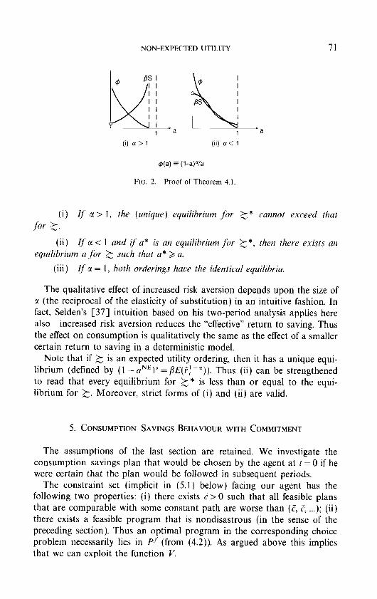
Thus the existence of equilibria follows from the properties of S represented in Fig. 2. Uniqueness is guaranteed when CI > 1, but multiple equilibria cannot be ruled out when c( < 1. (The c( = 1 case leads to a horizontal graph for /3S in Fig. 2.) These results are established rigorously in the context of the following theorem:

THEOREM 4.1. Under the assumptions maintained in this section, a stationary Nash equilibrium exists, and if CI > 1, it is unique.

Consider the effects of increased risk aversion. Let k* be more risk averse than 2. Denote by S* the function that corresponds to 2* via (4.4t(4.5). Then (3.10) implies S*(a)<S(a) on the relevant domain if c( < 1, and the reverse inequality is implied if o! L 1. Thus the following theorem is readily proven by a simple curve shifting exercise in Fig. 3.

THEOREM 4.2. Let 2* he more risk averse than 2 in the sense qf Definition 2.1.

I0 Henceforth we write V(Z) rather than V(F,).


Ml* fq ca 1 a 1

(i) a> 1 (ii) a< 1

@(a) = (l-a)Va

FIG. 2. Proof of Theorem 4.1.

(i) If (r > I, the (unique) equilibrium for 2 * cannot exceed that for 2.

(ii) If tl < 1 and if a* is an equilibrium for 2 *, then there exists an equilibrium a for 2 such that a* > a.

(iii) [ f c( = 1, both orderings have the identical equilibria.

The qualitative effect of increased risk aversion depends upon the size of 3t (the reciprocal of the elasticity of substitution) in an intuitive fashion. In fact, Selden’s [37] intuition based on his two-period analysis applies here also-increased risk aversion reduces the “effective” return to saving. Thus the effect on consumption is qualitatively the same as the effect of a smaller certain return to saving in a deterministic model.

Note that if 2 is an expected utility ordering, then it has a unique equilibrium (defined by (1 - aNE)’ = BE(?) -’ )). Thus (ii) can be strengthened to read that every equilibrium for k* is less than or equal to the equilibrium for 2. Moreover, strict forms of (i) and (ii) are valid.

5. CONSUMPTION-SAVINGS BEHAVIOUR WITH COMMITMENT

The assumptions of the last section are retained. We investigate the consumptionsavings plan that would be chosen by the agent at I = 0 if he were certain that the plan would be followed in subsequent periods.

The constraint set (implicit in (5.1) below) facing our agent has the following two properties: (i) there exists C > 0 such that all feasible plans that are comparable with some constant path are worse than (F, C, . ..). (ii) there exists a feasible program that is nondisastrous (in the sense of the preceding section). Thus an optimal program in the corresponding choice problem necessarily lies in P-’ (from (4.2)). As argued above this implies that we can exploit the function V.

72 CHEW AND EPSTEIN

The level of initial wealth can be normalized to elqual unity. Then we solve the optimization problem

,*I xC/?-‘[a,(,7)(1 -u,(,F))...(l -a,_,(,~,i))~,-..~,~, P>. (5.1)

2

where ,? denotes (Fo, . . . . F, ~ , ) for t 3 1, a, E (0, 1 ), and for each I 3 1, a,: [r, F]’ + (0, 1) is a measurable function.

The problem (5.1) can be solved in two stages and is equivalent to

(5.2)

p- max V I4.);; !

~w)iO)’ x+$--&

,CL, XC/J’ ‘[u,(,~)(l-u,(,7))...(1-u,~,(,~,~))r’,...?,~,

2 1’ g.

The consequences of increased risk aversion may be determined from (5.2). Simply note that if k* is more risk averse than 2, then the problem corresponding to the former ordering is similar to (5.2), but p* d ,u (by (3.10)). This leads immediately to the following theorem:”

THEOREM 5.1. Let k* he more risk averse than 2 in the sense of Defini- tion 2.1 and suppose that solutions exist to the uppropriute.forms of (5.1) for both orderings. Then the agent with the more risk averse ordering consumes no more (no less) than the other agent at t = 0 if c( 3 1 (c( < 1) and if consumption plans ,formuluted at t = 0 are binding for the entire future.

Note that the qualitative effect of increased risk aversion on consumption in the initial period is identical to that described in Theorem 4.2 for the case where commitment is impossible.

It is interest to compare the Nash equilibrium and commitment-optimal consumption levels at t = 0. Such a comparison follows immediately from (4.4) and (5.2) upon noting that p B H(u) for all a E (0, 1).

THEOREM 5.2. Suppose a,* solves (5.2) and let aNE be a Nash equilibrium. Then u,*<(a)uNE according us c1< ( 2 ) 1.

” The proofs of Theorems 5.1 and 5.2 are straightforward and are omitted.


Once again the degree CJ = 2-l of intertemporal substitutability is critical and it determines the relative magnitudes of a,* and aNE in the intuitively anticipated manner. The ability to commit increases the “effective return” to saving. Thus initial consumption is (weakly) higher with commitment if a< 1 and lower if a3 I.

6. CONCLUDING REMARKS

To date the primary reason for interest in non-expected utility theories has been their capability to explain behavioural paradoxes. We have shown that nonlinear theories can be a useful analytical tool in a consumptionsavings context since they permit the separation of risk aversion from the elasticity of substitution.

We noted in the introduction that expected utility models have not explained consumption and asset return data very well. It seems worthwhile to investigate whether the more flexible specifications proposed here would perform better. Such an empirical analysis would complement the recent impirical investigation in [ 1 l] based on recursive preference specifications which violate ordinal dominance.” First, however, the behavioural analysis of this paper would need to be extended to include many assets having returns with a more general serial structure.

Since the preference orderings considered in this paper are not intertemporally consistent, the implied behaviour depends on whether plans can be made which are binding on the future. Above we have considered the individual choice problem while taking the existence of institutions for making commitments to be exogenous. In future work we intend to investigate whether non-expected utility preferences can help to explain the existence of a variety of commitment institutions-for example, defined contribution pension plans-which are frequently rationalized by the ad hoc hypothesis of changing tastes or myopia.

APPENDIX

Proof of Theorem 3.1. Necessity of the axioms is obvious. We outline a proof of their sufficiency in the case c( # 1. For more details and the CI = 1 case, the reader is referred to [3].

Let V be the functional which represents 2 in the sense of (2.5).

” The Selden and Stux specification has been implemented by Hall [ 141 and Zin 1441. But their estimating equations are applicable only to a naive consumer who continually ignores the fact that plans formulated at any given time will not be carried out in the future.

74 CHEW AND EPSTEIN

* (by recursivity)

(c,p”) - (GPb)

+ (by recursiwty)

co,c and cl > 0. p’, pb and P E fvUL1”)

FIG. 3. Proof of Theorem 3.1.

Existence of V is implied by ordinal dominance as described in the statement of Theorem 3.2 and the discussion leading up to it. We wish to show that V coincides with the expected value functional on a suitable domain. First, we show that it satisfies the independence axiom (IA).

Refer to Fig. 3 and let j”, jb, and j be random variable consumption paths corresponding to the probability measures pU, pb, and p, respectively. Then the chain of implications in the figure implies that

It follows that V satisfies IA on an appropriate subdomain. By using compact continuity, an expected utility representation for V can be deduced. In fact, by the translation and scale invariance properties (3.7) and (3.8), V must be the expected value functional [27]. This representation for V can be extended to its entire domain by applying extendability. 1

Proof of Theorem 3.2. For any c>O, denote by (c) the constant path (c, c, c, . ..). Define V as follows:

4(c)) if (co7 PI - (~1

v44co3 P)) = + a if (co, p)>(c)Vc>O

--rx) if (c,, p)<(c) Vc > 0.


Then V is well-defined by ordinal dominance, and (3.5 ) and (3.9) can be verified. The invariance properties (3.6) and (3.8) may be established as described in the text. 1

For the behavioural analyses in Sections 4 and 5 we require some further continuity properties for 2. To formulate the first one we need another notion of convergence for sequences in M(I: + (6)). For any p E M(I’+ + (6)) denote by E[z4; p] the extended real-valued expected value of u taken from (3.1))(3.2). Say that p” +* p if both p” + p in the usual weak convergence topology and E[u: p”] + E[u; p]. Since p” +*p implies p” + p, the next continuity requirement is made weaker by use of the * convergence notion. For any L > 0, /1(0, L) denotes i(c): 0 < c < L,\, the set of deterministic constant consumption paths with consumption less than L. Since M(/1(0, L)) is homeomorphic to M((0, L)), first degree stochastic dominance may be defined on the former space in the natural fashion. Denote that dominance relation by FSD.

Limited Continuitj~. If {(c-l;, p”) j ; is a sequence in (0, co) x M(ii(0, L)) for some #CC > L > 0 such that

(i) c; -+ L’~ and p” +* p, c > 0, and p E M(A(0, L));

(ii) r;f > c’; + I 3 c0 and p” FSD p” + ’ FSD p for all n;

then for every (cb, p’)~ P which satisfies (c;, p’) > (co, p), there exists N such that n > N * (cl,, p’) > (c;l, p”).

On the other hand if (ii) is replaced by

(ii’) (~6. p”)< (c) for all c> 0 and for all n, then (c,, p)i (c) for all c > 0.

In contrast to compact continuity, limited continuity deals with measures whose supports are not bounded away from zero consumption. Such measures pose difficulties when CI 3 1 since ,f(c) is then unbounded below near 0. Limited continuity is not needed below when CY < 1.

The second additional continuity axiom in a sense requires continuity with respect to the consumption level along deterministic constant paths.

Certainty Continuity. For each (c,, P)E P, the sets (c: (c)> (co, p)> and (c: (c) < (c,, p)> are open in the real line.

LEMMA A.1. The ordering represented by V y defined in (2.4) satisfies certainty continuity and all of the axioms in Theorem 3.2. Moreover, limited continuity’ is also satisfied {f the probability transformation function g is concave und g’(0) < a.

76 CHEW AND EPSTEIN

As noted earlier the concavity of g is equivalent to the Yaari functional (2.2) being risk averse in the sense of conditional certainty equivalents, which in turn is equivalent to aversion to mean preserving increases in risk ([42]). Also, in conjunction with g’(0) < “~1, concavity implies the Lipschitz property

Ig(x’) - g(x)/ < A Ix’ - XI VXE [O, l] (A.1 1

for A = g’(0).

Proof: Only limited continuity requires attention. Assume (i) and (ii) of that axiom and let m” = c$(c;(, p”), m = $(c,, p). Note that

m” FSD m” + ’ FSD m for all n. CA.2)

We now show that

m” -+ m. CA.3 1

Each p” and p E M(/i(O, L)) induce in a natural fashion measures on the interval (0, JC). Denote those measures also by p” and p. Given d > 0 3_c > 0 such that

P(k, ml)> 1 -A. (A.41

Since p” FSDp, it follows also that

P”((c, ml)> 1 -A for all n. (A.51

Let f: ( - co, cx ) + ( - m, cc) be continuous and bounded by Ifl. By changing variables and subsequently by exploiting (A.4) and (A.5) we can write

I j f(z)d(m”(z)-m(z))

But the last term can be made small because c; -+ cO, { u(c;, (c)): n = 1, 2, . and _c < c < L} is a bounded set and pn -+ p. This proves (A.3).

Denote by V (rather than Vy) the rank-dependent functional defined in (2.2). We need to prove that

lim V(&) = V(m). (A.61


(In (2.2), V was defined on c.d.f.‘s; but it can also be identified with a function on probability measures, which identification is adopted in this proof.) If R < 1, then the m”‘s and m all have supports that lie within a bounded interval in [0, co). Thus (A.6) follows from the well-known continuity properties of the rank-dependent funcltional [a]. The only difficulty arises when x > 1 since then u is unbounded below as consumption in any period approaches zero.

If x > 1, then mfl and nz lie in M( [ - a, 0)). For any K > 0, denote by rni and mK the truncations to [ -K, 0) of nz” and m, respectively. Suppose that V(m) > --r;. (The argument is similar when V(m) = -a.) Given E > 0 3K such that

V(nz,)< V(m)+&.

Now nz$--+m, and the continuity of V noted above imply that V(m”,)+ V(m,). Thus 3N such that V(m”,)< V(m)+& for all n> N. But V(m”) < V’(m”,). Thus I’(&‘) < V(m) +E for all sufficiently large II. Also, V(nP) > V(m) because of (A.2). This proves (A.6).

For the second part of limited continuity, assume (i) and (ii’) of that axiom and define m” and m as above. Condition (ii’) is impossible if !x < 1. If we take CI > 1, then V from (2.2) need be considered only for measures with supports in the negative real line. Suppose for the moment that the Yaari functional V is such that for all such measures m,

V(m)= -1% if and only if Em= -m, (A.7)

where Em is the expected value of m. Then (ii’) a V(m”) = --rx; * Em”= -CU. Since p” +* p follows that Em=lim(Em”)= -cc and so by (A.7) V(m) = --a3 and (co. p) < (c) for all c > 0. Thus the proof is complete if (A.7) can be established.

The Lipschitz property (A.1 ) for g implies that I”- % z n(g[m(r)]) 2 AJO, = dm(z); that is

V(m) > AEm. CA.8 1

Also, g concave * g(x) 3 .Y on [0, l] 3 (by [42])

I’( m ) < Em. (A.9)

Together, (A.8) and (A.9) imply (A.7). 1

Proof of Theorem 4.1. For CI = 1, see [3]. We concentrate on TV # 1. For any given a and u* in (0, 1 ), let c0 = a and let pi be the probability

measure corresponding to the random path in which consumption in

78 CHEW AND EPSTEIN

period t3 1 is given by c’, = a*( 1 -a)(1 -a*)‘-’ i,,. . . i,-, if t> 1. Then p~M(l~+(6)) since by (4.1)

with probability one. If cI< 1. then

% xCP’[(l -a”)‘-’ qPE< cc, by (4.1).

Thus if a and a* are restricted to a compact interval inside (0, 1 ), then p? has support in [I ,C] lr for some 0 < I< L < cc. The critical properties of S portrayed in Fig. 2(ii) are now readily established. The continuity of S follows from compact continuity and its negative slope is implied by the FSD monotonicity of V. By the latter and (4.1), c’ -’ 6 V(r”AP”) d S(u) < C’~/~-‘(~)(‘-~‘)‘<CC on (0, 1). Thus S(O+)<cc and S(ll)>O.

When a > 1, f(c) is unbounded below near c = 0 and we must make use of limited continuity in order to establish the needed properties of S. For a~(0, l), let C (a) denote x;C fl’-‘[(l -uo)‘-’ ?,- I ...r”o]‘P”/(l -a). Define d-sup{u~ (0, 1): C (a)> -cc with probability l} and let m(u) be the probability measure corresponding to C (a). Define 5 E sup{u E (0, d): m(u) E $(P”), where P“ and 4 are defined in (4.2) and Theorem 3.2 respectively. Note that

~(m(a’)v O<u<Z (A.lO)

Let u” be given by (1 Yu”)‘Pz/?(EY”~Pr )= 1. For O<u<u’,EZ(u) converges to a finite number while for u” d a < 1, EC(a) diverges to - co. But EC(u) is continuous in a on (0, 1) in an extended real-valued sense.

It is straightforward to show that


Next we show that

WI(a) $! &P’ ). (A.ll)

Take {u”‘,?c(&~) such that a,,Jti. Then m(a”)+m(ti) in M((-so, cc)). There exists (co(Z), p(G)) and for each n !l(c,(a”), p(a”))~ (0, acl) x M(/i(O, L)) such that m(a”) = &~,(a”), ~(a”)) and m(E) = d(c,(a), p(a)), where L is independent of H. Moreover, in light of the convergence of m(8) to m(Z), the fact that m(u”)$&Pf) for all n, and the continuity of EC(u) noted above, we can choose the sequence ( (~,(a”), ~(a”))) ;^ so that it satisfies conditions (i) and (ii’) of limited continuity. Thus the latter =-(~,(a), p(a))<(c) for all c>O=E-(c,(a), ~(ti))$P’=(A.ll).

We wish to prove that S( .) defined by (A.lO) is continuous on (0,~) and that S(u) + cc: as a -+ 5. Consider the latter property. Let un T 2 and construct consumption programs (~,(a”), ~(a”)), (c,(a), p(a)) as above so as to satisfy conditions (i) and (ii) of limited continuity. By (A. 11) (c,(a), p(Z)) -K (c) for all c > 0. Thus limited continuity implies that for all c>o 3N, n>N~(c,(u’~),p(u”))~(L’)~V(WI(u~))<~C’~~/(1-~)(1-~). Thus V(m(u”)) converges to --cc; and S(8) converges to xi.

The desired continuity of S(-) follows in a similar fashion. 1

REFERENCES

1. S. H. CHEW, A generalization of the quasilinear mean with applications to the measure- ment of income inequality and decision theory resolving the Allais paradox, Econometrica 51 (1983), 1065-1092.

2. S. H. CHEW, An axiomatization of the rank-dependent quasilinear mean generalizing the Gini mean and the quasilinear mean, Working Paper 156, Johns Hopkins University, 1985.

3. S. H. CHEW AND L. G. EPSTEIN, Non-expected utility preferences in a temporal framework with an application to consumption-savings behaviour, Working Paper 8701, University of Toronto, 1987.

4. S. H. CHEW, L. G. EPSTEIN. AND U. SEGAL, Invariant mean values and measures of income inequality, mimeo, University of Toronto. 1989.

5. S. H. CHEW, E. KARNI. AND Z. SAFRA, Risk aversion in the theory of expected utility with rank-dependent probabilities, J. Econ. Theory 42 (1987), 37c381.

6. S. H. CHEW AND K. R. MACCRIMMON, Alpha utility theory: A generalization of expected utility theory, Faculty of Commerce and Business Administration Working Paper 669, University of British Columbia, 1979.

7. S. H. CHEW AND M. H. MAO, A Schur-concave characterization of risk aversion for nonlinear. nonsmooth continuous preferences. Working Paper 157, Johns Hopkins University, 1985.

8. J. P. DANTHINE AND J. B. DONALDSON. Stochastic properties of fast vs. slow growing economies, Econometrica 49 (1981). 1007-1034.

9. E. DEKEL, An axiomatic characterization of preferences under uncertainty. J. &on. Theor? 40 (1986), 304318.

10. L. G. EPSTEIN AND S. E. ZIN. Substitution, risk aversion and the temporal behaviour

80 CHEW AND EPSTEIN

of consumption and asset returns: A theoretical framework, Econometrica 57 (1989), 931-969.

11. L. G. EPSTEIN AND S. E. ZIN, Substitution, risk aversion and the temporal behaviour of consumption and asset returns: An empirical analysis, Working Paper 8718 revised, University of Toronto, 1989.

12. P. C. FISHBURN. Transitive measurable utility. J. Econ. Theor! 31(1983), 293-317. 13. J. GREEN, “Making book against oneself.” the independence axiom and nonlinear utility

theory, (&art. J. G.u~r. 102 (1987), 7855796. 14. R. HALL, Interest and consumption, NBER Working Paper 1694. 1985. 15. R. HALL, Consumption, NBER Working Paper 2265, 1987. 16. L. HANSEN AND K. SINCILETON. Stochastic consumption, risk aversion, and the temporal

behavior of asset returns, J. Polk &on. 91 (1983), 2499265. 17. T. H. JOHNSON AND J. B. DONALUSON, The structure of intertemporal preferences under

uncertainty and time consistent plans, Economerricu 53 (1985) 1451-1458. 18. E. KARNI AND 2. SAFRA, Ascending bid auction games: A nonexpected utility analysis,

Working Paper 20-87. Tel Aviv University, 1987. 19. R. E. KIHLSTROM AND L. J. MIRMAN, Risk aversion with many commodities, J. Econ.

Theory 8 (1974). 361-388. 20. T. C. KOOPMANS. Stationary ordinal utility and impatience. Economerrica 28 (1960).

287-309.

21. D. M. KREPS AND E. L. PORTEUS, Temporal resolution of uncertainty and dynamic choice theory, Econometrica 46 (1978). 185-200.

22. W. LEININGER. The existence of perfect equilibria in a model of growth with altruism between generations, Rev. Econ. Srud. 53 (1986), 349-368.

23. D. LEVHARI AND T. SRINIVASAN. Optimal savings under uncertainty, Rev. Econ. Stud. 36 (1969), 153-164.

24. R. E. LUCAS. Asset prices rn an exchange economy, Econometrica 46 (1978), 1429-1446. 25. M. J. MACHINA. “Expected utility” analysis without the independence axiom, Econometrica

50 (1982). 277-323.

26. M. J. MACHINA, The economic theory of individual behaviour towards risk: Theory. evidence and new directions, IMSSS Technical Report 433, Stanford University, 1983.

27. M. NAGUMO, Uber eine Klasse der Mittelwerte, Japun. J. Math. 7 (1930), 71-79.

28. B. PELEC AND M. E. YAARI. On the existence of a consistent course of action when tastes are changing, Rev. Econ. Sfud. 40 (1973). 391401.

29. R. A. POLLAK, Consistent planning, Rev. Econ. Bud. 35 (1968). 201-208.

30. J. QUIGGIN, Anticipated utility theory, J. Econ. Eehav. Organ. 3 (1982), 323-343.

31. T. RADER. “Microeconomic Theory,” Academic Press, New York, 1982. 32. H. RAIFFA. “Decision Analysis,” Addison-Wesley, Reading, MA, 1968. 33. H. L. ROYDEN. “Real Analysis,” Macmillan, New York. 1963. 34. P. A. SAMUELSON, Lifetime portfolio selection by dynamic stochastic programming, Rev.

Econ. Statist. 51 (1969). 239-246.

35. U. SEGAL, Axiomatic representation of expected utility with rank-dependent probabilities, Ann. Oper. Res.. Choice under Uncertainty, in press.

36. L. SELDEN. A new representation of preference over “certain x uncertain” consumption pairs: The “ordinal certainty equivalent” hypothesis, Econometrica 46 (1978). 1045-1060.

37. L. SELDEN. An OCE analysis of the effect of uncertainty on saving under risk preference independence, Rev. Econ. Stud. 46 (1979), 73-82.

38. L. SELDEN AND 1. STUX, Consumption trees, OCE utility and the consumption savings decision, Columbia University, 1978.

39. G. J. STIGLER AND G. S. BECKER, De gustibus non est disputandum, Amer. Econ. Rev. 67 (1977), 7690.


40. R. H. STROTZ, Myopia and inconsistency in dynamic utility maximization, Rev. Econ.

Stud. 23 (1956) 1655180. 41. R. H. THALER AND H. M. SHEFRIN. An economic theory of self-control, .I. Polit. Icon. 89

(1981). 392406. 42. M. E. YAARI, Univariate and multivariate comparisons of risk aversion: A new approach,

in “Uncertainty. Information and Communication: Essays in Honour of Kenneth J. Arrow” (W. P. Heller, R. M. Starr. and D. Starrett, Eds.), Cambridge Univ. Press, Cambridge, 1986.

43. M. E. YAARI, The dual theory of choice under risk, Econometrica 55 (1987), 955115. 44. S. E. ZIN. Intertemporal substitution, risk and the time series behaviour of consumption

and asset returns, Discussion Paper 695, Queen’s University, 1987.

nonexpected utility preferences in a temporal framework with...

Documents