Nonequilibrium electron dynamicsnear Mott transition

Sharareh Sayyad

In collaboration with: Martin Eckstein

Max Planck Institute for the Structure and Dynamics of Matter,University of Hamburg-CFEL, Hamburg, Germany

September 27, 2016

1

Photo induced Mott transition in 1T − TaS2

• Mott insulator at T=30 K

• Preparation of an excited state in crossover region↪→ Induced insulator-to-metal transition

Creation of hot carriers

Collapse of the gap < 100 fs

Fast thermalization < 100 fs

Relaxation of the excited state > 500 fs

Electronic relxation timescale< electron-lattice relxation timescale

� L. Perfetti, et al., Phys. Rev. Lett. 97, 067402 (2006).

2

Mott transition in the half-filled Hubbard model

H = −J∑

〈ij〉,σ

(c†iσcjσ + h.c.) + U

N∑

i=1

ni↑ni↓

U/W

(βW )−1

Metal

Insulator

Badmetal

-3 0 3

A(ω

)ω

U=4

β=1β=5

β=7

3

Relaxation to the Fermi liquid?

H = −J∑

〈ij〉,σ

(c†iσcjσ + h.c.) + U

N∑

i=1

ni↑ni↓

Preparing the system in the crossover region:

Excitation (quench)

Phys. Rev. Lett. 117, 096403(2016).

Fast thermalizationPhys. Rev. B 84, 035122(2011).

Studying the relaxation dynamics of the excited state

+electrons coupled to the environment

Σeb = λ U/W

(βW )−1

tcut

tf

Metal

Insulator

Crossover

4

Slow-relaxing electronic characteristic timescale

Solved by DMFT:

-3 0 3

A(ω

,t)

ω

β=3U=4, , λ=0.5

t=20t=50

-3 0 3

A(ω

,t)

ω

U=4, λ=0.5 β=10

t=20t=40t=80

Hubbard Bands :: Fast thermalization

→ inverse One-body energy-scales [ 14

]

Quasiparticle peak :: Slow retrieval (for β > 5)

→ timescale>> inverse One-body energy-scales [ 1

4]

>> inverse quasiparticle bandwidth [ 10.8

]

Bottleneck of dynamics (large β):

temperature-independent evolution of hqp

0.3

0.4

0.5

0.6

0.7

0.8

0.9

30 40 50 60 70 80

hq

p

time

U=4, λ=0.5

β=5β=6.5β=7.5

β=8β=10

5

Dynamical mean field theory

JU

lattice problem → impurity-bath problem

Solving the impurity problem

∆(t, t′)

t t′

DMFT self-consistency on Bethe lattice

Gimp(t, t′) ≡ ∑

kGlatt

k (t, t′)

Σlattk (t, t′) ≡ Σimp(t, t′)

ImpurityGlattk = 1

i∂t+µ−ǫk−Σlattk

solver

∆(t, t′) = J(t)Gimp(t, t′)J(t′)

approximation

Σimp, Gimp

Review on NEDMFT: Rev. Mod. Phys. 86, 779 (2014).

6

Impurity solver: U(1) slave-rotor

c†σ︸︷︷︸electron

= eiθ︸︷︷︸X:rotor

f†σ︸︷︷︸

spinon

⇔ Ge = GX .Gf

Atomic model:{|0〉, | ↑〉, | ↓〉, | ↑↓〉}︸ ︷︷ ︸

electron

≡ {|l = −1〉, |l = 0〉, |l = 0〉, |l = 1〉}︸ ︷︷ ︸Charge conservation: l=nf−1

⊗{|0〉, | ↑〉, | ↓〉, | ↑↓〉}︸ ︷︷ ︸

Spinon

On the impurity site:

Solving Dyson equations for

GX with ΣX = ∆.Gf

Gf with Σf = ∆.GX

Imposing constraints

Charge conservation

|X|2 = 1

Why slave-rotor impurity solver:

Accessibility of long time-evolution (Similar to NCA)

Accurate phase diagram near Mott transition (not the case in NCA)

� Equilibrium study: S. Florens and A. Georges, Phys. Rev. B. 66 165111 (2002).

� Nonequilibrium study: Sh. S and M. Eckstein, Phys. Rev. Lett. 117, 096403 (2016).

7

Equilibrium Physics: Slave-rotor Language

-3 0 3

A(ω

)

ω

U=4

β=1β=5

β=7

By decreasing the temperature:

Electron: height of the quasiparticle peak enhanced.

Rotor: density at zero frequency formed.

Spinon: nonmonotonous behavior as a function of β

-1

0

1

2

-4 -2 0 2 4

A(ω

)

ω

Af*0.2

β=1

a)

AfAx

-4 -2 0 2 4

ω

Af*0.04

β=5

b)

-4 -2 0 2 4

ω

Af*0.2

β=7

c)

Maximum in the spinon inverse bandwidth

0

60

120

180

240

0 2 4 6 8 10

τ eq

β

λ=0.5U=4

U=4.1U=4.2

U=4.25U=4.3

Footprint of this nonmonotonous response out of equilibrium ?

8

Spinon’s response: presence of a “⋂

” turn!

0

0.1

0.2

0.3

0.4

0.5

0 20 40 60 80 100 120

Gfre

t (t,t-s

)

s

U=4, λ=0.5, β=10

t=16

t=32

t=48

t=62

t=80

t=96t=112

t=128

9

Spinon’s response: presence of a “⋂

” turn!

0

0.1

0.2

0.3

0.4

0.5

0 20 40 60 80 100 120

Gfre

t (t,t-s

)

s

U=4, λ=0.5, β=10

t=16

t=32

t=48

t=62

t=80

t=96t=112

t=128

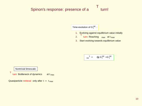
Time-evolution of Gretf :

1. Evolving against equilibrium value initially

2. “⋂

” turn: Reaching τmax at tmax

3. Start evolving towards equilibrium value

Nontrivial timescale:

“⋂

” turn: Bottleneck of dynamics at tmax

Quasiparticle retrieval only after t = tmax

τ−1ne = −∂sGret

f /Gretf

0

150

300

25 50 75

τn

e

t

s=16

U=4

U=4.1

U=4.2

U=4.25

U=4.3

10

Spinon “⋂

” turn: equilibrium and nonequilibrium

0

60

120

180

240

0 2 4 6 8 10

τ eq

β

λ=0.5

U=4U=4.1U=4.2

U=4.25U=4.3

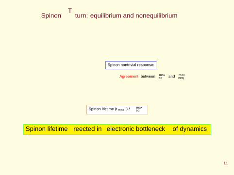
Spinon nontrivial response:

Agreement between τmaxeq and τmax

neq

Spinon lifetime (tmax)∝ τmaxeq

Spinon lifetime reflected in electronic bottleneck of dynamics

11

Reflection of spinon lifetime in other observables?

Assume : =Gf (ω) ≈ δ(ω)/π

τ−1ne = −Σ

′′f (ω = 0) ≈ −πJ2 ∫

dωA(ω)A(ω)

cosh2(βω/2)

Emergence of a correlation timescale

0

60

120

180

240

300

0 2 4 6 8 10

τ eq

β

λ=0.5

U=4U=4.2U=4.3

Nontrivial spinon response in multi-orbital physics:

“Frozen” spin-spin correlation functionPh. Werner, et al., Phys. Rev. Lett. 101,166405 (2008).

Non-Fermi-liquid behavior of optical conductivity in perovskite ruthenates (∝ 1/√ω)

Y. S.Lee, et al., Phys. Rev. B 66, 041104 (2002).

12

Conclusion and Summary

• Study the Hubbard model near Mott transition

• Investigate the system under a quick ramp

• slave-rotor impurity solver + DMFT

Gimp(t, t′) ≡ ∑k G

lattk (t, t′)

Σlattk (t, t′) ≡ Σimp(t, t′)

ImpurityGlatt

k = 1i∂t+µ−ǫk−Σlatt

k solver

Slow retrieval of the quasiparticle density

Presence of a “⋂

” turn in the spinon retarded Green’s function

Presence of a nonmonotonous spinon behavior in equilibri1um

Agreement between equilibrium and nonequilibrium spinon response

0

60

120

180

240

300

0 2 4 6 8 10

τ eq

β

λ=0.5

U=4U=4.2U=4.3

Emergence of a correlation timescale

13

Thanks for your attention.

14