Nondeterministic Operators inAlgebraic Frameworks 

Sigurd Meldal Michal Walicki

Technical report CSL–TR–95–664Program Analysis and Verification Group Report No. 69

March 1995

Computer Systems LaboratoryDepartment of Electrical Egineering and Computer Science

Stanford UniversityStanford, CA 94305–4055

AbstractA major motivating force behind research into abstract data types and algebraic specifications is the realizationthat software in general and types in particular should be described (“specified”) in an abstract manner. Theobjective is to give specifications at some level of abstraction: on the one hand leaving open decisions regardingfurther refinement and on the other allowing for substitutivity of modules as long as they satisfy a particularspecification.

The use of nondeterministic operators is an appropriate and useful abstraction tool, and more: nondeter-minism is a natural abstraction concept whenever there is a hidden state or other components of a system de-scription which are, methodologically, conceptually or technically, inaccessible at a particular level of abstrac-tion.

In this report we explore the various approaches to dealing with nondeterminism within the framework ofalgebraic specifications. The basic concepts involved in the study of nondeterminism are introduced. The mainalternatives for the interpretation of nondeterministic operations, homomorphisms between nondeterministicstructures and equivalence of nondeterministic terms are sketched, and we discuss various proposals for, re-spectively, the initial and terminal semantics. We make some comments on the continuous semantics of non-determinism and the problem of solving recursive equations over signatures with binary nondeterministicchoice. And we then go on to present the attempts at reducing reasoning about nondeterminism to reasoning infirst order logic, and gives an example of a calculus dealing directly with nondeterministic terms. Finally, re-writing with nondeterminism is discussed: primarily as a means of reasoning, but also as a means of assigningoperational semantics to nondeterministic specifications.

Key Words and Phrases: Algebraic specifications, nondeterminism, formal methods, software design, founda-tions of computer science, programming language semantics.

Copyrigh © 1995by

Sigurd MeldalMichal A. Walicki

CONTENTSINTRODUCTION . . . . . . . . . . . . . . . . . . . . . . . . . . . . . . . . . . . . . . . . . . . . . . . . . . . . . . . . . . . . . . . . . . . . . . . . . . . . . . . . . . . . . 1

1. BASIC CONCEPTS . . . . . . . . . . . . . . . . . . . . . . . . . . . . . . . . . . . . . . . . . . . . . . . . . . . . . . . . . . . . . . . . . . . . . . . . . . . . . . . . . 2Nondeterminism and nondeterminacy ...................................................................................... 2Nondeterminism and underspecification ................................................................................... 2Representational vs. “real” nondeterminism ............................................................................. 2Bounded and unbounded nondeterminism ................................................................................. 4Biased agents ...................................................................................................................... 4Singular and plural .............................................................................................................. 6Etc. ... ................................................................................................................................ 6Notation ............................................................................................................................. 7

2. SEMANTIC PRELIMINARIES . . . . . . . . . . . . . . . . . . . . . . . . . . . . . . . . . . . . . . . . . . . . . . . . . . . . . . . . . . . . . . . . . . . . 72.1. OPERATIONS ... ................................................................................................................ 8

Functional models................................................................................................................ 8Multialgebras...................................................................................................................... 9Power algebras ..................................................................................................................10Relational models................................................................................................................11

2.2. ... HOMOMORPHISMS ... ....................................................................................................12Element homomorphisms. .....................................................................................................13Multihomomorphisms...........................................................................................................13Power homomorphisms. .......................................................................................................13

2.3. ... AND EQUIVALENCIES. ..................................................................................................14Element equality .................................................................................................................14Set equality ........................................................................................................................14Consistency relation ............................................................................................................15

3. INITIAL MODELS & SPECIFICATION LANGUAGES . . . . . . . . . . . . . . . . . . . . . . . . . . . . . . . . . . . . . . . . . 173.1. CHOICE AS A PRIMITIVE – SET UNION................................................................................183.2. INCLUSION......................................................................................................................193.3. PARTIAL ORDERS ............................................................................................................203.4. LATTICES AND UNIFIED ALGEBRAS...................................................................................213.5. THE PRICE OF INITIALITY .................................................................................................24

4. TERMINAL MODELS. . . . . . . . . . . . . . . . . . . . . . . . . . . . . . . . . . . . . . . . . . . . . . . . . . . . . . . . . . . . . . . . . . . . . . . . . . . . . 27

5. SOLUTIONS OF RECURSIVE EQUATIONS – CONTINUOUS MODELS.. . . . . . . . . . . . . . . . . . . . . 285.1. DETERMINISTIC PRELIMINARIES.......................................................................................295.2. CPOS FOR NONDETERMINISTIC CHOICE.............................................................................30

6. REASONING SYSTEMS . . . . . . . . . . . . . . . . . . . . . . . . . . . . . . . . . . . . . . . . . . . . . . . . . . . . . . . . . . . . . . . . . . . . . . . . . . 336.1. REDUCTION TO DETERMINISM..........................................................................................346.2. CALCULUS OF NONDETERMINATE TERMS..........................................................................35

7. OPERATIONAL MODELS AND REWRITING . . . . . . . . . . . . . . . . . . . . . . . . . . . . . . . . . . . . . . . . . . . . . . . . . . 377.1. NON-CONFLUENCE AND RESTRICTED SUBSTITUTIVITY.......................................................377.2. REWRITING LOGIC...........................................................................................................407.3. REASONING AND REWRITING WITH SETS. ..........................................................................43

8. SUMMARY. . . . . . . . . . . . . . . . . . . . . . . . . . . . . . . . . . . . . . . . . . . . . . . . . . . . . . . . . . . . . . . . . . . . . . . . . . . . . . . . . . . . . . . . . 44

9. REFERENCES . . . . . . . . . . . . . . . . . . . . . . . . . . . . . . . . . . . . . . . . . . . . . . . . . . . . . . . . . . . . . . . . . . . . . . . . . . . . . . . . . . . . . 45

1

IntroductionMathematics never saw much of a reason to deal with something called “nondeterminism.” Itworks with values, functions, sets, relations. In computing science, on the other hand, non-determinism has been an issue from the very beginning, if only in the form of nondetermin-istic Turing machines or nondeterministic finite state machines. Early references to nonde-terminism in computer science go back to the sixties [38, 84]. A great variety of theories andformalisms dealing with it have been developed during the last two decades. There are thedenotational models based on power domains [103, 117, 51, 106], the predicate transform-ers for the choice construct [29, 30, 104, 118], modifications of the l-calculus [73, 4, 49].Nondeterminism arises in a natural way when discussing concurrency, and models of con-currency typically also model nondeterminism. There are numerous variants of process lan-guages and algebras [13, 89, 90, 50, 54, 52, 65, 39, 11], event structures [136, 135, 134, 2],state transition systems [83, 71], Petri nets [100, 109].

In terms of modeling nondeterminism may be considered a purely operational notion.However, one of the main reasons for considering nondeterminism in computer science is theneed for abstraction, allowing one to disregard irrelevant aspects of actual computations.Typically, we prefer to work with models which do not include all the details of the physicalenvironment of computations such as timing, temperature, representation on hardware, etc.Since we do not want to model all these complex dependencies, we may instead representthem by nondeterministic choices. The nondeterminism of concurrent systems usually arisesas an abstraction of time. Similarly nondeterminism is also a means of increasing the level ofabstraction when describing sequential programs [85, 130], and as a way of indicating a“don’t care” attitude as to which among a number of computational paths will actually beutilized in a particular evaluation [30].

The variety of approaches referred to above indicates the possible difficulties in gatheringall the pieces into one uniform theory, let alone a short presentation. In this paper we areconcerned with algebraic specifications and hence will consider only a part of the whole pic-ture of nondeterminism. As far as the basic notions related to nondeterminism and the asso-ciated algebraic formalisms are concerned, the paper is by and large self-contained. Only oc-casionally references to other areas presupposing some prior knowledge will be made.

In section 1 the basic concepts involved in the study of nondeterminism are introduced.Sections 2-5 discuss the semantic issues, and 6-7 reasoning with nondeterminism. The mainalternatives for the interpretation of nondeterministic operations, homomorphisms betweennondeterministic structures, and equivalence of nondeterministic terms are sketched in 2.Sections 3 and 4 discuss various proposals for, respectively, the initial and the terminal se-mantics. In section 5 we make some comments on the continuous semantics of nondeter-minism and the problem of solving recursive equations over signatures with binary nonde-terministic choice. 6 presents the attempts at reducing reasoning about nondeterminism toreasoning in first order logic and then gives an example of a calculus dealing directly withnondeterministic terms. In 7 rewriting with nondeterminism is discussed: primarily, as ameans of reasoning, but also as a means of assigning operational semantics to nondeter-ministic specifications.

2

1. Basic conceptsIn this section we present informal definitions of the basic concepts and distinctions involvedin the study of nondeterminism.

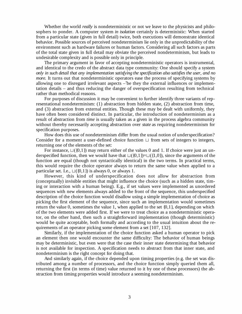
Nondeterminism and nondeterminacyRoughly speaking, nondeterminacy concernssyntax, nondeterminism semantics. The con-structs which always yield unique result aredeterminate, those which may yield differentresults when invoked several times nondeter-minate. The presence of a nondeterminate con-struct in an expression does not force the corre-sponding operation to be nondeterministic.Determinacy implies determinism but nonde-terminacy does not necessarily imply nondeter-minism and, as observed in [18], the problemwhether a nondeterminate term is deterministicor not is, in general, undecidable. We are pri-

marily concerned with the intentional nondeterminism originating from the presence in thelanguage of some constructs which have nondeterministic semantics.

Nondeterminism and underspecificationWhen developing a software system in a number of refinement steps, we are often interestedin specifying the functionality of the system uniquely but only with respect to some relevantproperties. That is, each model of the specification is a standard (deterministic) structure butwe do not identify one unique model. We then speak of underspecification. Later in the de-velopment process we may add more properties, whenever we find it appropriate, and so re-strict the model class. Thus underspecification functions also, like nondeterminism, as ameans of abstraction. It bears a resemblance to nondeterminism in that it leaves open thepossibility of choosing among several admissible models. The important difference betweenthe two notions may be roughly expressed thus: underspecification admits a choice betweendifferent models but nondeterminism admits choices within one model. While underspecifi-cation fits into the concepts of classical logic and model theory smoothly, the treatment ofnondeterminism leads to complications and, typically, requires introduction of non-standardfeatures both into the models and logic. For this reason some researchers postulate the use ofunderspecification as the primary, if not the only, means of abstraction. Others consider itinsufficient and try to design formalisms which capture the phenomenon of nondeterminismas distinct from underspecification.

Representational vs. “real” nondeterminismThere are essentially two reasons why one might want to include the concept of nondeter-minism in the traditional algebraic specification methods:(1) Real nondeterminism.

The system being specified really is nondeterministic – its behavior is not fully predictable,nor fully reproducible, no matter how detailed our knowledge of its initial state.

(2) Representational (or pseudo-) nondeterminism [64, 121, 130].The behavior of the system being specified may be fully predictable in its final imple-mentation (i.e. deterministic), but it may not be so at the level of abstraction of the specifi-cation.

Though many think of representational nondeterminism as identical to underspecification,they turn out to be technically and conceptually quite distinct (as we shall see shortly).

nondeterminate

determinate

deterministicnondeterministic

3

Whether the world really is nondeterministic or not we leave to the physicists and philo-sophers to ponder. A computer system in isolation certainly is deterministic: When startedfrom a particular state (given in full detail) twice, both executions will demonstrate identicalbehavior. Possible sources of perceived nondeterminism lie only in the unpredictability of theenvironment such as hardware failures or human factors. Considering all such factors as partsof the total state given in full detail may obviate the perceived nondeterminism, but leads toundesirable complexity and is possible only in principle.

The primary argument in favor of accepting nondeterministic operators is instrumental,and identical to the credo of the abstract data type community: One should specify a systemonly in such detail that any implementation satisfying the specification also satisfies the user, and nomore. It turns out that nondeterministic operators ease the process of specifying systems byallowing one to disregard irrelevant aspects – be they the external influences or implemen-tation details – and thus reducing the danger of overspecification resulting from technicalrather than methodical reasons.

For purposes of discussion it may be convenient to further identify three variants of rep-resentational nondeterminism: (1) abstraction from hidden state, (2) abstraction from time,and (3) abstraction from external entities. Though these may be dealt with uniformly, theyhave often been considered distinct. In particular, the introduction of nondeterminism as aresult of abstraction from time is usually taken as a given in the process algebra communitywithout thereby necessarily accepting abstraction over state as requiring nondeterminism forspecification purposes.

How does this use of nondeterminism differ from the usual notion of underspecification?Consider for a moment a user-defined choice function t from sets of integers to integers,returning one of the elements of the set:

For instance, t({0,1}) may return either of the values 0 and 1. If choice were just an un-derspecified function, then we would have that t({0,1})=t({1,0}), since the arguments of thefunction are equal (though not syntactically identical) in the two terms. In practical terms,this would require the choice operator always to return the same value when applied to aparticular set. I.e., t({0,1}) is always 0, or always 1.

However, this kind of underspecification does not allow for abstraction from(conceptually) invisible entities that might influence the choice (such as a hidden state, tim-ing or interaction with a human being). E.g., if set values were implemented as unorderedsequences with new elements always added to the front of the sequence, this underspecifieddescription of the choice function would disallow using a simple implementation of choice aspicking the first element of the sequence, since such an implementation would sometimesreturn the value 0, sometimes the value 1, when applied to the set {0,1}, depending on whichof the two elements were added first. If we were to treat choice as a nondeterministic opera-tor, on the other hand, then such a straightforward implementation (though deterministic)would be quite acceptable, both formally and according to the usual intuition about the re-quirements of an operator picking some element from a set [107, 132].

Similarly, if the implementation of the choice function asked a human operator to pickan element then one would encounter the same difficulty: The behavior of human beingsmay be deterministic, but even were that the case their inner state determining that behavioris not available for inspection. A specification needs to abstract from that inner state, andnondeterminism is the right concept for doing that.

And similarly again, if the choice depended upon timing properties (e.g. the set was dis-tributed among a number of processors, and the choice function simply queried them all,returning the first (in terms of time) value returned to it by one of these processors) the ab-straction from timing properties would introduce a seeming nondeterminism.

4

The implementation relation also arises in the distinction between loose and tight rela-tionships between structures modeling nondeterministic operators (see below).

Bounded and unbounded nondeterminismBounded nondeterminism refers to the case where every terminating computation has only afinite number of possible results; unbounded – to the one where the set of the possible resultsmay be infinite.

It may be argued [30, 54] whether unbounded nondeterminism has a plausible compu-tational interpretation. A deterministic program P which takes a natural number n as inputand outputs a natural number m corresponds to a partial recursive function. The relation

RP(n,m) ⇔ P(n)=m

is recursively enumerable (RE), and the subset LP of natural numbers for which P does notterminate is co-recursively enumerable. For nondeterministic program P, the input-outputrelation RP(n,m) is also RE, but when the involved nondeterminism is unbounded LP is muchmore complex than co-RE. Firstly, (non-)termination cannot be guaranteed and LP is the setof those inputs on which P may not terminate. Then it is shown in [25] that for erratic (seebelow) unbounded nondeterminism LP has the complexity ( 1

1. This either presents a seriouschallenge to the Church-Turing thesis and the classical notion of computability or, perhaps,discredits unbounded nondeterminism as a notion without computational relevance. Never-theless, even if one might agree that the notion of unbounded nondeterminism is not feasiblefrom the implementation point of view, it may even so provide an invaluable abstractionmechanism at the specification level.

Unbounded nondeterminism creates severe difficulties in models based on fixed pointsemantics because, unlike bounded nondeterminism, it is not continuous in the standardconstructions of power domains. However, it should be observed that noncontinuity is notcaused by the nondeterminism, but rather by the unboundedness. Noncontinuity may alsoarise in a determinate language, for instance, in a language admitting quantification over infi-nite sets.

Biased agentsThe paradigmatic concept of nondeterminism is probably that of arbitrary choice. Choosingnondeterministically between a and b there is a possibility that we get a and also a possibilitythat we get b. The choice may be influenced by additional factors which nevertheless leave it,to some extent, undetermined. If this is the case we may speak of the (agent making the)choice being biased.

The most extensively studied case of such agents involves bias with respect to possibletermination. Erratic choice is completely arbitrary – it may happen that such a choice willlead to a nonterminating computation and it may happen that it will eventually producesome result. Angelic choice, on the other hand, will always avoid branches which may lead tonontermination. If there is a computational path leading to a successful result, angelic non-determinism will guarantee that such a path will be found. Finally, a demonic choice will dothe opposite and always follow the path, if such exists, leading to a nonterminating computa-tion.

In terms of implementation, erratic nondeterminism is the least problematic. A choicemay be performed locally without consideration of the possible consequences of the choicesmade. It may be also thought of as an unpredictable environment beyond the control of theprogram. An operational intuition of angelic nondeterminism [25] can be a system which,whenever a choice is to be made, spawns several new processes, one for each among the pos-sible results of the choice. The first process to terminate causes all other processes to stop aswell. The demonic case can be analogous except that every process must terminate if the

5

whole computation is to terminate. Demonic nondeterminism is in [21] called backtracknondeterminism – it is there thought of as a system which makes a choice and follows thepath until it terminates. If it does, the system backtracks to the point at which the last choicewas made and follows another path. It will terminate only after having checked that all possi-ble choices lead to terminating computations.

The terms erratic, angelic, demonic are used not only to refer to the termination aspectbut, generally, to the situations where nondeterminism involves arbitrary choices where theresults are either “desirable” or “undesirable,” e.g., with respect to definedness.

The first version of angelic nondeterminism [84] was related to this kind of preferencefor “desirable” behavior. It was local (like the erratic one) in the sense that it chose among itsarguments looking only at their values rather than at the consequences of its own choice. Ifboth arguments were well defined (completed computations) any of them might have beenchosen erratically but if any of the arguments was undefined the other one was chosen.

This is an example of the value bias [110] where every agent may have its own preferenceas to which values to choose. Such a bias can be modeled by a partial order on the values ex-pressing the preferences. An agent presented with the choice between a and b first considerswhether any of the values is to be preferred (is greater in the ordering), in which case thisvalue is selected. Otherwise the choice is arbitrary. For instance, the ordering for the angelicagent in the last paragraph would be the flat partial order: a≤b iff a=⊥ ∨ a=b.

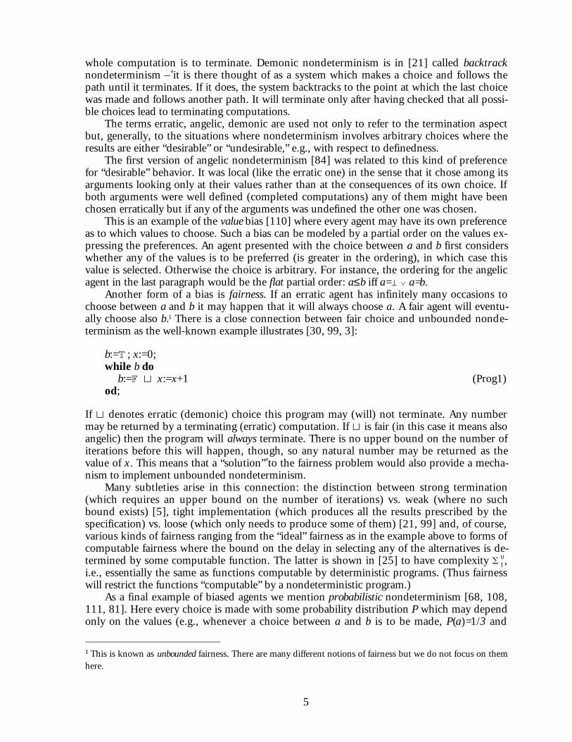
Another form of a bias is fairness. If an erratic agent has infinitely many occasions tochoose between a and b it may happen that it will always choose a. A fair agent will eventu-ally choose also b.1 There is a close connection between fair choice and unbounded nonde-terminism as the well-known example illustrates [30, 99, 3]:

b:=T ; x:=0;while b do

b:=F t x:=x+1 (Prog1)od;

If t denotes erratic (demonic) choice this program may (will) not terminate. Any numbermay be returned by a terminating (erratic) computation. If t is fair (in this case it means alsoangelic) then the program will always terminate. There is no upper bound on the number ofiterations before this will happen, though, so any natural number may be returned as thevalue of x. This means that a “solution” to the fairness problem would also provide a mecha-nism to implement unbounded nondeterminism.

Many subtleties arise in this connection: the distinction between strong termination(which requires an upper bound on the number of iterations) vs. weak (where no suchbound exists) [5], tight implementation (which produces all the results prescribed by thespecification) vs. loose (which only needs to produce some of them) [21, 99] and, of course,various kinds of fairness ranging from the “ideal” fairness as in the example above to forms ofcomputable fairness where the bound on the delay in selecting any of the alternatives is de-termined by some computable function. The latter is shown in [25] to have complexity ( 1

0,i.e., essentially the same as functions computable by deterministic programs. (Thus fairnesswill restrict the functions “computable” by a nondeterministic program.)

As a final example of biased agents we mention probabilistic nondeterminism [68, 108,111, 81]. Here every choice is made with some probability distribution P which may dependonly on the values (e.g., whenever a choice between a and b is to be made, P(a)=1/3 and

1 This is known as unbounded fairness. There are many different notions of fairness but we do not focus on themhere.

6

P(b)=2/3), or also on the agents making the choice (so that PM(a,b) for an agent M may differfrom PN(a,b) for another agent N.) Of course, the formalism for the description, as well as themodels, of probabilistic nondeterminism are considerably more complex than the formalismsand models of non-probabilistic nondeterminism. They are probably more appealing to thecommunity interested in probabilistic algorithms than to workers in the field of formal speci-fications and abstract data types.

Singular and pluralIn deterministic programming the distinction between call-by-value and call-by-name se-mantics is well-known. The former corresponds to the situation where the actual parametersto function calls are evaluated and passed as values. The latter allows also parameters whichare function expressions, passed by a kind of Algol copy rule [113], and which are evaluatedonly when a need for their value arises.

The nondeterministic counterparts of these two notions are what [110] calls singular andplural semantics of parameter passing. Other, very closely related distinctions go under thenames call-time-choice vs. run-time-choice [26, 49, 50], inside-out (IO) vs. outside-in (OI)[34, 35]. The different names reflect slight differences in meaning of the concepts. Exceptwhere we are entering into a more detailed discussion of this distinction (7) we will adopt theterminology [110] (taking the risk of abusing it a bit for the sake of a more intuitive exposi-tion).

The terminology of [110] reflects the meaning of the nondeterminate terms as repre-senting sets of possible results. Evaluation of such a term yields a unique result, hence whenevaluation of the argument is required at the moment of the call it represents a single value.When a term is passed by some variant of the textual copy rule and several evaluations of itin the body of the operation can happen independently of each other, then we can picturethe situation as passing the whole set of possible results where each reference to the parame-ter name picks (independently) one among the possible results.

Etc. ...Among other, more particular distinctions which may be occasionally referred to, we have:Weak vs. strong [110]. Weak nondeterminism means that, although some internal parts of a

computation may happen nondeterministically, the eventual result is uniquely determinedby the input. For instance, confluent rewriting of a term may apply different rules (chosennondeterministically) but will always arrive at the same normal form; a term may be calledweakly nondeterministic if it is nondeterminate and deterministic. Strong nondeterminismis, of course, the nondeterminism proper.

Tight vs. loose [99, 21, 110]. This distinction concerns the relation between two, possiblynondeterministic, structures. If M is one of them and displays some nondeterminism thenN is said to be tight if it displays exactly the same amount of nondeterminism, and it isloose if its nondeterminism is, possibly, more restricted than of M. For instance, if M is aspecification then, typically, its implementation N will be allowed to decrease the nonde-terminism of some operations (loose). Similarly, if M is a programming language withnondeterminate constructs, then we may think of a (loose) deterministic implementationN of M as being correct if every operation in N returns a result which is among the possi-ble results of the corresponding operation in M.

Restrained vs. unrestrained [110]. The former is nondeterminism of single programming con-structs – “choose arbitrary number”, and the latter is nondeterminism allowing choice ofdifferent execution paths – “goto label1 or label2”. The latter can be easily implementedusing the former. Nevertheless, the names come from the fact that denotational models ofthe latter are much more complex and require power domain construction over functionspaces with a non-flat ordering.

7

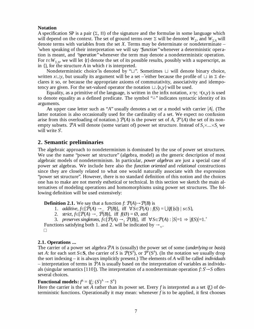
NotationA specification SP is a pair ((, P) of the signature and the formulae in some language whichwill depend on the context. The set of ground terms over ( will be denoted W(, and W(,X willdenote terms with variables from the set X. Terms may be determinate or nondeterminate – when speaking of their interpretation we will say “function” whenever a deterministic opera-tion is meant, and “operation” whenever the term may denote a nondeterministic operation.For t∈W(,X, we will let {t} denote the set of its possible results, possibly with a superscript, asin {}, for the structure A in which t is interpreted.

Nondeterministic choice is denoted by “t”. Sometimes t will denote binary choice,written xty, but usually its argument will be a set – either because the profile of t in ( de-clares it so, or because the appropriate axioms of commutativity, associativity and idempo-tency are given. For the set-valued operator the notation t.{x,y} will be used.

Equality, as a primitive of the language, is written in the infix notation, x=y; =(x,y) is usedto denote equality as a defined predicate. The symbol “$” indicates syntactic identity of itsarguments.

An upper case letter such as “A” usually denotes a set or a model with carrier _A_. (Thelatter notation is also occasionally used for the cardinality of a set. We expect no confusionarise from this overloading of notation.) P(A) is the power set of A, P+(A) the set of its non-empty subsets. PA will denote (some variant of) power set structure. Instead of S1×...×Si wewill write Si.

2. Semantic preliminariesThe algebraic approach to nondeterminism is dominated by the use of power set structures.We use the name “power set structure” (algebra, model) as the generic description of mostalgebraic models of nondeterminism. In particular, power algebras are just a special case ofpower set algebras. We include here also the function oriented and relational constructionssince they are closely related to what one would naturally associate with the expression“power set structure”. However, there is no standard definition of this notion and the choicesone has to make are not merely esthetical or technical. In this section we sketch the main al-ternatives of modeling operations and homomorphisms using power set structures. The fol-lowing definition will be used extensively:

Definition 2.1. We say that a function f: P(A)→P(B) is1. additive, f∈[P(A) →∪ P(B)], iff ∀S∈P(A) : f(S) = U{f({s}) | s∈S},2. strict, f∈[P(A) →+ P(B)], iff f(Ø) = Ø, and3. preserves singletons, f∈[P(A) →1 P(B)], iff ∀S∈P(A) : _S_=1 ⇒ _f(S)_=1. 

Functions satisfying both 1. and 2. will be indicated by →].¤

2.1. Operations ...The carrier of a power set algebra PA is (usually) the power set of some (underlying or basis)set A: for each sort S∈S, the carrier of S is P(SA), or P+(SA). (In the notation we usually dropthe sort indexing – it is always implicitly present.) The elements of A will be called individuals– interpretation of terms in PA is usually based on the interpretation of variables as individu-als (singular semantics [110]). The interpretation of a nondeterminate operation f: Si→S offersseveral choices.

Functional models: fA = {fz: (Si)A → SA}

Here the carrier is the set A rather than its power set. Every f is interpreted as a set {fz} of de-terministic functions. Operationally it may mean: whenever f is to be applied, it first chooses

8

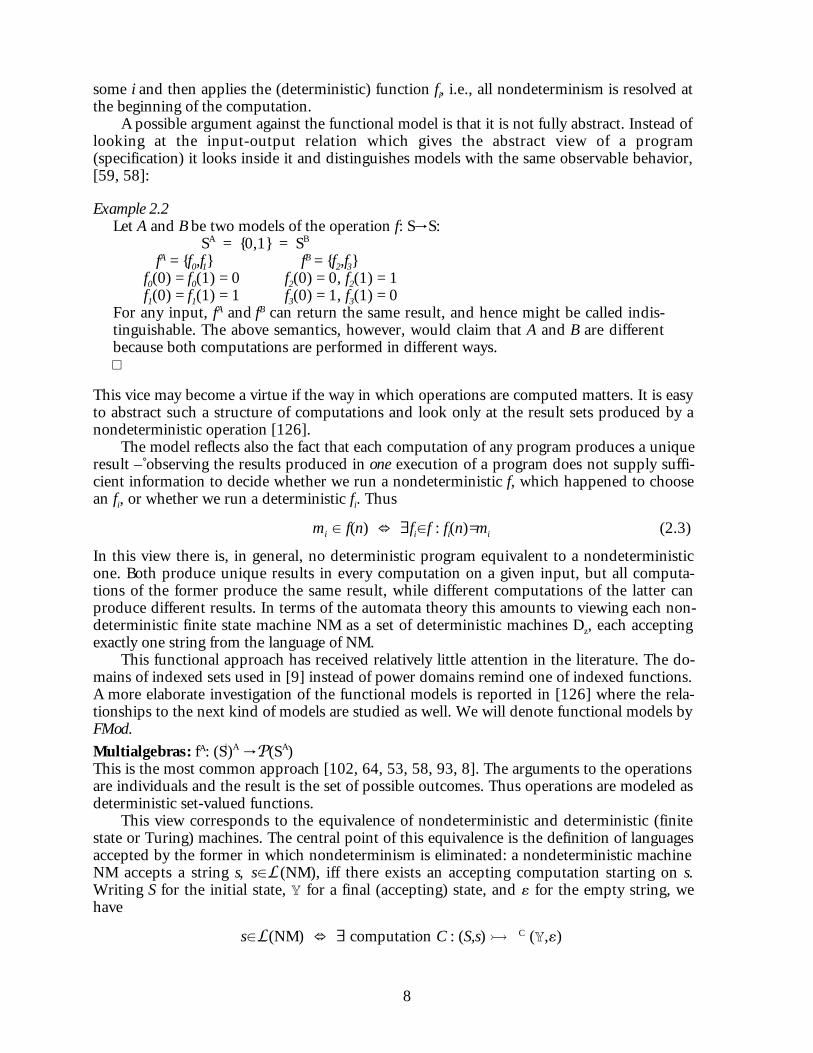
some i and then applies the (deterministic) function fi, i.e., all nondeterminism is resolved atthe beginning of the computation.

A possible argument against the functional model is that it is not fully abstract. Instead oflooking at the input-output relation which gives the abstract view of a program(specification) it looks inside it and distinguishes models with the same observable behavior,[59, 58]:

Example 2.2Let A and B be two models of the operation f: S→S:

SA = {0,1} = SB

fA = {f0,f1} fB = {f2,f3}f0(0) = f0(1) = 0 f2(0) = 0, f2(1) = 1f1(0) = f1(1) = 1 f3(0) = 1, f3(1) = 0

For any input, fA and fB can return the same result, and hence might be called indis-tinguishable. The above semantics, however, would claim that A and B are differentbecause both computations are performed in different ways.¤

This vice may become a virtue if the way in which operations are computed matters. It is easyto abstract such a structure of computations and look only at the result sets produced by anondeterministic operation [126].

The model reflects also the fact that each computation of any program produces a uniqueresult – observing the results produced in one execution of a program does not supply suffi-cient information to decide whether we run a nondeterministic f, which happened to choosean fi, or whether we run a deterministic fi. Thus

mi ∈ f(n) ⇔ ∃fi∈f : fi(n)=mi (2.3)

In this view there is, in general, no deterministic program equivalent to a nondeterministicone. Both produce unique results in every computation on a given input, but all computa-tions of the former produce the same result, while different computations of the latter canproduce different results. In terms of the automata theory this amounts to viewing each non-deterministic finite state machine NM as a set of deterministic machines Dz, each acceptingexactly one string from the language of NM.

This functional approach has received relatively little attention in the literature. The do-mains of indexed sets used in [9] instead of power domains remind one of indexed functions.A more elaborate investigation of the functional models is reported in [126] where the rela-tionships to the next kind of models are studied as well. We will denote functional models byFMod.

Multialgebras: fA: (Si)A →P(SA)This is the most common approach [102, 64, 53, 58, 93, 8]. The arguments to the operationsare individuals and the result is the set of possible outcomes. Thus operations are modeled asdeterministic set-valued functions.

This view corresponds to the equivalence of nondeterministic and deterministic (finitestate or Turing) machines. The central point of this equivalence is the definition of languagesaccepted by the former in which nondeterminism is eliminated: a nondeterministic machineNM accepts a string s, s∈L(NM), iff there exists an accepting computation starting on s.Writing S for the initial state, Y for a final (accepting) state, and « for the empty string, wehave

s∈L(NM) ⇔ ∃ computation C : (S,s) ½ C (Y,«)

9

The existential quantifier eliminates all nondeterminism – it does not matter any more whichcomputation is performed; an accepting computation C either exists or not, and the languageof NM is uniquely defined. Hence, an equivalent deterministic machine DM can be con-structed by “dovetailing” all possible computations of NM. Analogously, if f is a(nondeterministic) multioperation, the result set f(n) can be computed deterministically byevaluating (“dovetailing”) all possible computation paths, as it is done for the Turing ma-chines.

Composition of multioperations is defined using the following simple fact [34, 106]:

Proposition 2.4. For every f: A→P(B) there exists a unique fP: P(A)→]P(B) (strict,additive) such that the following diagram commutes: A

{_}↙ ↘ f

P(A) f P

→ P(B)¤

{_} denotes the canonical embedding sending every element to the singleton set. Thus com-position is defined as: g(f(x)) = gP(f(x)) = U{g(e) | e∈f(x)}. Also here it is natural to interpret thecarrier as the set A rather than its power set, but the canonical embedding {_} and additivityof the operations make the transition between the two very easy. We will denote multimodelsby MMod.

Here the two models from example 2.2 would be identified, since both fA and fB appliedto any argument return the set {0,1}.

In most cases, one lets an operation f map A to P+(B) rather than P(B). The former cor-responds to the total while the latter to the partial models in which f(a)=Ø indicates that f isundefined on a. With the above definition of composition this partial interpretation impliesangelic nondeterminism.

Example 2.5Let the sort N = {0,1,2} and S={a,b,c}, and the operations f: N→S, g: S→N be suchthat

f(0) = {a,b} g(a) = {0,1}f(1) = {a,c} g(b) = {2}f(2) = Ø g(c) = Ø

Theng(f(0)) = {0,1,2}g(f(1)) = gP(f(1)) = gP({a,c}) = {0,1} ∪ Ø = {0,1}g(f(2)) = Ø

¤

To obtain more flexibility in modeling biased nondeterminism with multialgebras some ad-ditional constructions in the specification language are needed, analogous to those for parti-ality in the deterministic case, e.g., the bottom element ⊥ [77, 63, 91], or definedness predi-cate [21, 18, 59, 58].

Although the classes MMod and FMod are not isomorphic there is a strong sense of cor-respondence between the two:

Proposition 2.6 [127]. Every functional algebra F determines a multialgebra M andvice versa.

10

Proof:Let F be a functional algebra where fF = {f1, f2,...}. Define the multialgebra M by:• _M_ = _F_• fM(x) = {fi(x)|fi∈fF}.The reverse implication is analogous, though a bit more technical and not construc-tive:• _F_ = _M_For every f and m∈_F_ (of appropriate sort), let kf,m denote the cardinality of the setfM(m), and let kf =

Um

kf,m. Then, for every m there is a surjectionam: kf → fM(m)

and we define• fF = {fi | i≤kf } where, for every m, fi(m)=am(i).(Note that F isn’t unique and the axiom of choice is needed to actually determine it.)¤

Treatment of partiality in a functional model will be quite different from that illustrated inexample 2.5. Unless we introduce a ⊥ element (or a definedness predicate) explicitly, therewill be no default interpretation of undefinedness (such as the empty set) in the carrier of afunctional model.

Other consequences of the multialgebraic interpretation can best be explained by con-trasting it with the third possibility:

Power algebras: fA: P(S1A)×...×P(Si

A) →P(SA)Here every function takes a set as an argument and returns a set as the result. There are stilltwo possible ways to interpret this:

a) Every element of the result set is a possible outcome of applying the operation to any ele-ment of the argument set. Under this interpretation a power algebra is just a more conciseexpression of a multialgebra, as the following straightforward consequence of the proposition2.4 shows ([A→B] denotes the partial order of functions from A to B ordered pointwise):

Proposition 2.7. [A→P(B)] ' [P(A) →] P(B)].

b) The other (and from now on the only) meaning is that every element of the result set is apossible outcome of applying the operation to the argument set. Without any additional con-ditions such a definition begs the whole question of nondeterminism because what we obtainis a deterministic structure which just happens to have a power set as the carrier. In particu-lar, there is no distinction between elements, or 1-element sets, and other sets. An operation fmay, for instance, be such that f({0,1,2}) = {0} and f({0}) = {0,1}. This is counterintuitive [33,103] because one expects that an increase in the nondeterminism of the arguments to an op-eration should not result in a decreased nondeterminism of the result.

To meet the intuitive understanding one would require that the operations in a power al-gebra be ⊆-monotonic. ⊆-monotonicity does not imply additivity, and so proposition 2.7does not yield an isomorphism with multialgebras. The possibility of non-additive functionsbetween power sets offers new possibilities. If we aim at plural semantics of parameter pass-ing [110, 130] we are forced to allow the arguments of functions to be sets (and to let vari-ables refer to sets rather than individuals).

Example 2.8Let f be the operation

f(x) = if x=x then 0 else 1.

11

In any multimodel (x will refer to an individual and) the result set of f will be {0} forall x. In particular, {f(atb)}={0}. Some authors [77, 53] focus on the purely semanticissues, i.e., do not consider any specification language. But by adopting the multi-model of operations they are forced to adopt the singular semantics of the operationsymbols.If, on the other hand, we take f as mapping sets to sets, we obtain

f(atb) = if atb=atb then 0 else 1,which may give {f(atb)}={0,1}.¤

Actually, the last equality does not follow by itself in a power model, but depends further onthe interpretation of the equality atb=atb (which may be interpreted as element- or set-equality). We discuss this further in 2.3 and 7. The singular semantics can be obtained, ac-cording to 2.7, if we impose the additional restriction of additivity. Thus power algebras, butnot multialgebras, give us the possibility to define both singular and plural semantics.

The reasons why this approach is relatively unpopular in spite of its apparent generalityare probably mostly pragmatic and similar to the reasons why call-by-name semantics hasbeen superseded by the call-by-value in the deterministic setting (besides the fact that addi-tive function spaces have nicer formal properties). It may be argued that programs written interms of call-by-value are significantly clearer and more tractable than those using call-by-name. It should be also observed that one risks obtaining only uncountable models wheremost elements are unreachable when defining the carrier as a set of all (also infinite if the ba-sis set is infinite) subsets.

Power models will be denoted by PMod.

Relational models: fA ⊆ S1A×...×Si

A×SA

Although relational structures are well known in the universal algebra [27, 80, 79] they havenot quite found their way into the world of algebraic specifications, where the intuition offunctional application and its result plays the central role. Use of relations in semantic defini-tions is made in [99, 7, 93, 25, 18], and, in a categorical setting, in [119]. In so far as input-output behavior is concerned the relational models are isomorphic to multimodels.

Proposition 2.9. [A→P(B)] ' [A →(B→Bool)] ' [A×B → Bool] ' P(A×B).

With the relational product as the definition of composition, one obtains angelic nondeter-minism as with multialgebras (example 2.5). The most typical use of relations is for describ-ing termination properties and this is how they are used in [99, 7, 93, 25, 18]. One intro-duces a pair of relations: one for defining the input-output relation for the terminating com-putations, and one for characterizing the inputs which may (will) lead to divergence.

At the level of specifications, [121, 64, 21, 18] pointed in the direction of the relationalstructures by describing nondeterministic operations by means of characteristic predicates. Butthe relations are used as auxiliary definitions of the semantics and are not fully integrated intothe formalism of the specification language. None of the above works developed a relationalspecification language. An exception is the work from [1, 55, 123] which attempts to developa theory of data types based on the notion of a relation instead of a function. The relationallanguage leads to concise, albeit hard to read, specifications and gives powerful support inperforming calculations. Since nondeterminism is implicit in the notion of a relation – functions being just a special case of relations – the relational approach offers a uniformtreatment of deterministic and nondeterministic operations.

12

2.2. ... homomorphisms ...Homomorphisms for multialgebras were defined already in [101,102], and then in [45, 53,59, 64, 93].

Recall that a homomorphism w between (deterministic) structures A and B is a family ofmappings wS: S

A→SB for every S∈S such that the following diagram commutes for every f∈F:

(Si)A f A

→ SA

wSi ↓ ↓ wS

(Si)B f → SB

i.e., 1. for every constant c: →S wS(cA) = cB, and

2. for every operation f: Si→S wS(fA(xi)) = fB(wSi

(xi)) for all xi∈S iA

The transition to nondeterministic structures again introduces several possibilities of gener-alization. They are only loosely related to the choice of interpretation of the operations. Onegeneral remark applies to all of them: Since f is set-valued the result of following the leftmostpath in the diagram gives a set {fB(w(a))}. Similarly, {fA(a)} is a set and hence the result of ap-plying w to it (all its members) will give a set. The two basic possibilities are therefore:

tight homomorphism: {w(fA(a))} = {fB(w(a))} (2.10)

loose homomorphism: {w(fA(a))} ⊆ {fB(w(a))} (2.11)

Any of these two conditions may replace the homomorphism condition 1.-2. Loose homo-morphisms correspond to nonincreasing nondeterminism in the pre-image. Notice that thisdoes not preclude the cardinality of the set {fA(a)} being greater than this of {fB(w(a))}. Thensome values produced by fA(a) must be equivalent under w. Loose homomorphisms (or theirequivalents) are often used as the implementation criteria since it is generally accepted thatone should allow deterministic (less nondeterministic) implementations of nondeterministicdata types [121, 64, 94, 53, 132].

Both kinds of homomorphisms are used in the literature, though often under differentnames. The vocabulary becomes even more confused since many authors introduce the parti-ality considerations into the definitions. ([59, 18]. See [21, 93, 94] for more detailed andidiosyncratic notions.)

Element homomorphisms: w: A→B.This is the most common way of defining homomorphisms in a nondeterministic context,and we will denote it by EHom. Here the basic entities are individuals and homomorphismssend individuals to individuals. If multialgebras or power algebras are involved one still mayuse this notion of homomorphism since pointwise extension then defines the mapping be-tween the corresponding power sets. In either case the homomorphism condition will bemodified to (2.10) or (2.11).

Multihomomorphisms: w: A→P+(B).In [59] the element homomorphisms are generalized to the set-valued ones. There is at leastone advantage to be gained from this. In the deterministic case the initial structure for a givensignature ( is the collection of all words, W(. The interpretation of ( in a structure A is givenby the (unique) homomorphism I: W(→A. In the nondeterministic case we may want to in-terpret some terms as sets. The notion of multihomomorphisms makes such an interpretationa homomorphism whereas element homomorphisms do not.

I may be a homomorphism in EHom if we do not explicitly distinguish individuals fromsets. Then, if a structure B happens to be a power algebra, the mapping I: W(→B will actuallysend terms to sets since here B is the power set of some set. But then sets, which are the in-

13

terpretations of terms, cannot be identified with the result sets since the distinction betweenindividuals and sets disappears (sets are individuals in P(B)).

Multihomomorphism will be denoted by MHom.

Power homomorphisms: w: P(A)→P(B).This notion may lead to the peculiarities reminiscent of those of unrestricted (to ⊆-monotonic) functions in power algebras. The intention behind the definition of a homomor-phism is to make the mappings from individuals to individuals and from sets to sets“compatible”, even if the specification language is insufficient for dealing with this distinc-tion. Both EHom and MHom ensure such “compatibility” – mapping from a power set is ob-tained by pointwise extension of the mapping from individuals.

Example 2.12Suppose that ( contains only two constants of sort S, 0 and 1. Let A and B be thefollowing power algebras:

A=P{ 0 , a , b } B=P{ 0 , 1 } 0A={ 0 }, 1A={ a , b } 0B={ 0 }, 1B={ 1 }A power homomorphism w: A→B must send { 0 } to { 0 } and { a , b } to { 1 }. The rest isarbitrary so, for instance, we may have w({ a })=w({ b })={ 0 }.¤

This does not look very plausible. Again, as in the case of the power functions, it helps a lot ifwe insist that homomorphisms be ⊆-monotonic. But the point is how such a requirement isexpressed. If we just restrict the legal morphisms to those which are ⊆-monotonic then wewill exclude mappings which, like the one above, preserve the (-structure and satisfy thecompatibility condition defining homomorphisms.

It can be seen from the example that the trouble arises from the fact that we do not havea syntactic operation which would correspond to the semantic operation of set construction.Choice is not really such a constructor. If interpreted as set union, it would enable us to con-struct only the set { 0 , a , b } in A but not, for instance { a }. Thus, instead of extending the gapbetween syntax and semantics we might consider extending the specification language withan appropriate operation (predicate) such that the homomorphism condition wrt. to this op-eration would imply ⊆-monotonicity. Several works [77, 59, 87, 91] introduce such an op-eration. If, in addition, the language contains a predicate expressing that something is an in-dividual [91] then homomorphisms are again determined by the images of singletons. Thisleads to the same class of mappings as EHom since strict, additive mappings from P(A) toP(B) which, in addition, preserve singletons are isomorphic to the mappings from A to B:

Proposition 2.13. [A→B] ' [P(A) →],1 P(B)].

See also [102, 106] for the results concerning the relationship between various forms ofmappings between power sets. Extending the notational analogy with the models we will de-note the power homomorphisms by PHom.

2.3. ... and equivalencies.Although it might seem natural that = should be interpreted in power set structures as setequality (since the operations return sets) it is not obvious that the natural choice is the bet-ter.

Element equalityFirst of all, the sets returned by the operations represent possible results. But each particularapplication of every operation will return only one unique result. Thus, for instance, if

14

{s}={0,1} and {t}={0,1} it may very well happen that one application of s returns 0 while anapplication of t returns 1. One may require that two equal terms always return the same re-sults. This element equality reflects a strict view of observability – two terms are equal only ifthey are necessarily equal, i.e. they are deterministic and always return identical results. Thisnotion of equality corresponds to the function oriented model and, like that model itself, hasnot received much attention in the literature (except for [127, 133, 130]). Its apparent odditylies in the fact that, since a nondeterministic operation may return different results at differ-ent invocations, it is not even an equivalence relation. This reflects the lack of referentialtransparency which is intrinsic to nondeterministic operators.

Set equalitySlight variations of the set equality have been applied by many authors: under the name ofideal congruence in [102], extraction equivalence in [53, 121], observational equivalence in[64]. Variations concern mainly whether one uses plain set equality or whether the relation isdefined in the context of observability. In the latter case there are hidden and visible sorts,and terms s and t are extraction equivalent iff sets returned by all visible contexts C[_] whenapplied to s and t are equal.1 The simplest definition says that an equivalence relation E is ex-traction equivalence iff

∀(t,s)∈E, ∀C[_]∈W(,{x}, ∀a∈{C[t]} ∃b∈{C[s]} : (a,b)∈E (2.14)

The following result is then reported in [53, 102]:

Theorem 2.15. Let SP be a specification, M a multimodel, E an extraction equiva-lence on M , and [x] the E-equivalence class of x∈M. Then M/E is a multimodel,where

• the carrier of M/E is the set of E-equivalence classes { [x] | x∈_M_ }

• fM/E([x]) = Uy x∈[ ]

{ [a] | a∈fM(y) }.

¤

There is, of course, an implicit assumption about the form of the axioms in SP. In [102] SP isjust a signature, but if axioms are also present, as in [53], then the theorem does not hold infull generality. For the deterministic models, it is shown in [74], that the model class of SP isclosed under homomorphic images iff all the axioms of SP are positive formulae. It is easy toconstruct an example with inequality among the axioms which will show that M/E, for agiven multimodel M, is not necessarily a multimodel. It is not therefore unreasonable to ex-pect that the result from [74] will generalize to multimodels.

The importance of this nice counterpart of the analogous result for the deterministicequational classes is further diminished by the fact that one is still left with the problem ofconstructing a multimodel (the initial one?) from which one could start taking quotients.

Consistency relationEquality interpreted as set equality means that two terms are equal if they possibly can returnthe same results. It does not, however, guarantee that they will. In terms of an arbitrary actualobservation it does not guarantee anything. Following this line of thought of “the possible,”one arrives at the notion of the equality as the sheer prospect that two terms may conceivablyhappen to return the same result.

1 We do not focus on the distinction between visible and hidden sorts which, though formally important,would only add unecessary details to the presentation.

15

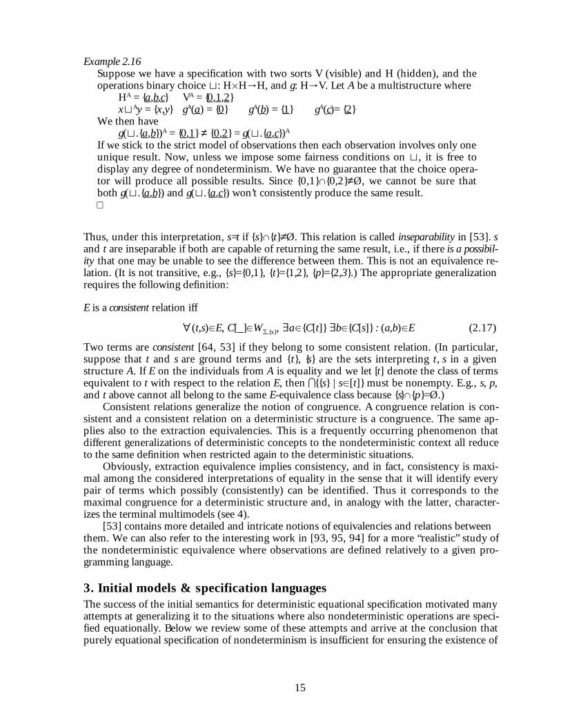
Example 2.16Suppose we have a specification with two sorts V (visible) and H (hidden), and theoperations binary choice t: H×H→H, and g: H→V. Let A be a multistructure where

HA = { a , b , c } VA = { 0 , 1 , 2 }xtAy = {x,y} gA( a ) = { 0 } gA( b ) = { 1 } gA( c )= { 2 }

We then haveg(t.{ a , b })A = { 0 , 1 } ≠ { 0 , 2 } = g(t.{ a , c })A

If we stick to the strict model of observations then each observation involves only oneunique result. Now, unless we impose some fairness conditions on t, it is free todisplay any degree of nondeterminism. We have no guarantee that the choice opera-tor will produce all possible results. Since {0,1}∩{0,2}≠Ø, we cannot be sure thatboth g(t.{ a , b }) and g(t.{ a , c }) won’t consistently produce the same result.¤

Thus, under this interpretation, s=t if {s}∩{t}≠Ø. This relation is called inseparability in [53]. sand t are inseparable if both are capable of returning the same result, i.e., if there is a possibil-ity that one may be unable to see the difference between them. This is not an equivalence re-lation. (It is not transitive, e.g., {s}={0,1}, {t}={1,2}, {p}={2,3}.) The appropriate generalizationrequires the following definition:

E is a consistent relation iff

∀(t,s)∈E, C[_]∈W(,{x}, ∃a∈{C[t]} ∃b∈{C[s]} : (a,b)∈E (2.17)

Two terms are consistent [64, 53] if they belong to some consistent relation. (In particular,suppose that t and s are ground terms and {t}, {s} are the sets interpreting t, s in a givenstructure A. If E on the individuals from A is equality and we let [t] denote the class of termsequivalent to t with respect to the relation E, then I{{s} | s∈[t]} must be nonempty. E.g., s, p,and t above cannot all belong to the same E-equivalence class because {s}∩{p}=Ø.)

Consistent relations generalize the notion of congruence. A congruence relation is con-sistent and a consistent relation on a deterministic structure is a congruence. The same ap-plies also to the extraction equivalencies. This is a frequently occurring phenomenon thatdifferent generalizations of deterministic concepts to the nondeterministic context all reduceto the same definition when restricted again to the deterministic situations.

Obviously, extraction equivalence implies consistency, and in fact, consistency is maxi-mal among the considered interpretations of equality in the sense that it will identify everypair of terms which possibly (consistently) can be identified. Thus it corresponds to themaximal congruence for a deterministic structure and, in analogy with the latter, character-izes the terminal multimodels (see 4).

[53] contains more detailed and intricate notions of equivalencies and relations betweenthem. We can also refer to the interesting work in [93, 95, 94] for a more “realistic” study ofthe nondeterministic equivalence where observations are defined relatively to a given pro-gramming language.

3. Initial models & specification languagesThe success of the initial semantics for deterministic equational specification motivated manyattempts at generalizing it to the situations where also nondeterministic operations are speci-fied equationally. Below we review some of these attempts and arrive at the conclusion thatpurely equational specification of nondeterminism is insufficient for ensuring the existence of

16

an initial model. Some more refined tools – at the syntactic as well as semantic level – areneeded.

Consider an equational specification SP which is supposed to be given a power algebrasemantics. As we have observed, power algebras are deterministic structures, and further-more, any standard model of SP may be considered a power model by identifying all ele-ments with 1-element sets and extending the operations pointwise. Thus, any equationalspecification will have a power model which is initial in the category (PMod,PHom). Butwhat is missing in such a model is nondeterminism. The crucial thing for the semantics ofnondeterminism is the distinction between the individuals and the sets of individuals whichgets completely lost in PMod and PHom. In fact, an initial power model need not consist of1-element sets. Any sets will do, since distinct sets are just distinct elements in PMod andPHom map sets to sets without considering their elements.

The semantic distinction may be introduced in various ways, for instance, by taking(PMod,MHom) or (PMod,EHom). In the former case, the same (deterministic) model as in(PMod,PHom) will be initial (provided MHom are tight), so things do not really get muchmore exciting. In the latter case, the deterministic power term structure will not be initial anymore, since there will be several element homomorphisms from a model interpreting everyterm as a 1-element set to a model where some terms are interpreted as sets with more thanone element.

What is needed is a closer relationship between the intuitive meaning of the power setstructures (i.e., sets as the result sets of the operations) and the syntactic means of specifyingthe relations reflected in such structures.

3.1. Choice as a primitive – set unionA “minimalist” approach [63, 77] admits two primitives in the specification language: equal-ity, which is interpreted as set equality, and binary choice which is specified by the join axi-oms:

J: xty = ytx (JC)xt(ytz) = (xty)tz (JA)xtx = x (JI)

Sometimes one also introduces a bottom element – the empty set [50] – and postulates dis-tributivity of t [63, 91]:

J1: xt⊥ = x (JE)f(..,xty,..) = f(..,x,..) t f(..,y,..) (JD)

Notice that the last axiom ensures singular semantics. So far, we have not done anything new– t is just a new deterministic operation specified equationally.

To make it into a choice one may attempt to require that t is to be interpreted as set un-ion. This, however, goes awry very quickly:

Example 3.1.aThe specification with three constants 0,1,2 and the axiom 0t1 = 0t(1t2) has noinitial model. For, constants must be interpreted as singletons { 0 },{ 1 },{ 2 },1 and t isset union, so I(0t1) = { 0 , 1 } and I(0t(1t2)) = { 0 , 1 , 2 }. In order to make these twosets equal we have to identify 2 with 0 or 1 . Either choice leads to the situation wherethere is no homomorphism to the model obtained by realizing the other choice. Also,since choice is set union we cannot take I(0t1) to be the set { 0 , 1 , 2 }.¤

1 Actually, this depends on the definition of power set structure and homomorphism we are working with.PMod would give the possibility of interpreting them as arbitrary sets. They have to be different sets, though,and so the problem would persist anyway.

17

The problem arises from the fact that one has decided in advance what the meaning of tshould be. Since it is the set union there is no other way to make the sets I(0t1) andI(0t(1t2)) equal than by identifying 2 with 1 or 0 . Taking the quotient of the term struc-ture or interpreting 0t1 as the set { 0 , 1 , 2 } are excluded. Thus axioms affecting the semanticsof choice may introduce inconsistency (albeit not a logical one) with this pre-defined mean-ing.

The axioms J1 are given in [63] without requiring the interpretation of t as set union.Then, of course, all equational specifications will have initial models, but this again is at theprice of loosing control over the distinction between deterministic and nondeterministic op-erations. Nevertheless, conditions are given (in terms of the associated rewriting systems) un-der which initial models of such specifications are isomorphic to the expected multimodelswith t interpreted as set union. The conditions (left-linearity and t-freeness, see 7) amountto forbidding situations like the one from the example – t-freeness, for instance, disallowsequating two terms which both contain occurrences of t.

The problem from example 3.1.a actually has two parts: One is that choice obtains somefixed semantics. Set union is perhaps not the best one and we will see in a moment otherpossibilities. The other is that the specification language does not provide sufficiently flexiblemeans for introducing new, nondeterministic operations by reference to this primitive one.Equations are symmetric and affect equally both sides. Introduction of a new operation, f,defined by f=0t1, and f=0t(1t2) would lead to the same problem. Thus each new equationis a potential source of a conflict.

It turns out that an increase in the expressive power of the specification language is re-quired. Some refinement of the equational language is needed for ensuring that choice will bea nondeterministic operation if this is not secured by some predefined semantics. A moreflexible language is needed to distinguish between the equivalence of two terms and the factthat one denotes only a (more deterministic) possible result of the other.

3.2. InclusionSince = is interpreted as set equality it shouldn’t do much harm if we instead made use of setinclusion as the primitive relation between terms [59, 58, 127, 133, 130]. Hußmann suppliesa very constructive generalization in [59, 58] where he introduces appropriate rewritingtechniques. Inclusion is the only primitive operation in the language of [59, 58]. There speci-fications are sets of inclusion rules (we shall keep “⊆” as denoting set inclusion in the struc-tures and use “≺” for the corresponding syntactic relation):

Example 3.1.b1) 0 ≺ t.{0,1}, 1 ≺ t.{0,1}2) 0 ≺ t.{0,1,2}, 1 ≺ t.{0,1,2}, 2 ≺ t.{0,1,2}

Notice that choice is no longer a primitive operation. The problematic axiom now be-comes:

3) t.{0,1}  ≺ t.{0,1,2} (writing  ≺ for two inclusions)The initial model is given by the following interpretation

4) I(c) ={ c }, for c=0,1,25) I(t.{0,1}) = I(t.{0,1,2} = { 0 , 1 , 2 }

¤

Since we have inclusions instead of equality in 1) the (initial) interpretation of t.{0,1} can beexpanded if necessary – here it contains 2 besides 1 and 2 . Choice is no longer primitive - thesemantics of sets is built into the semantics of ≺. In the initial (term) model, any term t is in-terpreted as the set of [s] such that s≺t, where [s] is the equivalence class of s, i.e., the set ofall p such that s ≺p.

18

However, to ensure the existence of the initial models some assumptions about thespecification must be made [59, 58]. One is that the specification has to possess a determi-nistic basis, i.e., a set of terms which are interpreted as singletons, and such that every termcan be reduced to at least one deterministic term (DET-completeness). To express this apredicate DET is introduced into the language, where DET(t) is valid if the term t is determi-nistic. Another assumption (DET-additivity) implies that arguments in the right hand sides ofinclusions must be deterministic. For instance, instead of 0≺f(1t2) we must write 0≺f(1)and 0≺f(2). Under these assumptions, every specification has a (loosely) initial model in(MMod,MHom) which can be constructed as in the above example. (These conditions arefurther discussed in section 7.)

3.3. Partial ordersInstead of sticking to the set interpretation one may generalize the fact that the set union(choice) is join operator. That is, instead of set union we can speak about join, instead of in-clusion – about a partial order.

The first work exploring these ideas in an algebraic framework is [77]. Given the axiomsJ (from 3.1) and a language with = and t, one can define a structure on the models reflectingthe intended nondeterministic interpretation. For each sort in the signature (, the result par-tial order on the word structure W(, ≺, is defined [77, 49]:

R: s≺t iff 1. s $ t or2. t $ sts1 or3. s $ f(pi), t $ f(ri), and pi≺ri

This definition amounts to the standard definition of a partial order on a lattice extendedwith the monotonicity axiom 3. which ensures that an increase in nondeterminism of the ar-guments never decreases the nondeterminism of the result. Note that the singularity axiomJD does not follow from J+R. We only have that R3 implies f(...,x,...) t f(...,y,...) ≺f(...,xty,...), reflecting our intuition that whatever can be produced under singular semanticscan also be produced under the plural one.

Equational specifications with t (and the axioms J) are just classical equational specifi-cations and hence always possess initial models. These models are essentially deterministicand nondeterminism is encoded as the additional structure ≺ implied by the occurrences oft. However, ≺ is not a part of the specification language.

Example 3.2.aLet us suppose that we want to add a new operation f to the specification (J) with thefollowing axioms:

1) f(x1,x2,x3) = x1tx2tx3

2) f(0,1,2) = f(0,0,1)We will obtain an initial model where 0t1 = 0t1t2. This does not cause the prob-lems of example 3.1.a since we now have a deterministic structure and merely takequotients of such structures. However, as a result we will obtain that 2 ≺ 0t1 holds,which is perhaps not quite what we had in mind.¤

It may be slightly surprising that defining a new operation has such consequences for theoriginal structure. After all, writing 1) and 2) we might be interested not in changing the se-mantics of choice but only in defining a new nondeterministic operation which behaves a lit-tle differently in some cases - for instance, so that it never returns some “forbidden” values.This illustrates the failure of this “deterministic” approach to reflect, in the general case, theintended meaning of nondeterministic choice as set union. The specification from example

19

3.2 does not conform to the restrictions from [63] mentioned at the end of 3.1 which makemodels of specifications with = and t isomorphic to the intended models where t is inter-preted as set union.

The collapse of the original ordering results here from the exclusive use of equations. Theapproach from 3.2 can easily accommodate such a situation. Using inclusions instead ofequality and making t a defined operation allows one to specify the nondeterministic opera-tions directly.

Example 3.2.bThe corresponding specification would be:

1) xi ≺ f(x1,x2,x3), for i=1,2,32) f(0,1,2) Â ≺ f(0,0,1)

The initial interpretation will assign the set { 0 , 1 , 2 } to both f(0,1,2) and f(0,0,1). Thisdoes not affect semantics of other operations, like t, which are specified independ-ently.¤

The resulting partial order ≺ is introduced in [77] in addition to the continuous struc-ture on the models needed for finding the solutions of recursive systems of equations. Wedevote section 5 to this topic and will continue the discussion of the present work there. Atthis point we may only remark that as the consequence of using continuous algebras themodel class is no longer closed under substructures and quotients. Thus initial models cannot be constructed simply as quotients of the word structure.

3.4. Lattices and unified algebrasThe approach discussed above introduced axioms for the join operation and defined(implicitly) the corresponding partial order. Example 3.2.a-b indicated that it might be ad-vantageous to reflect the semantically defined partial order in the specification language. Thisleads us directly to the lattice structures. In a very general form, they have been proposed asthe theoretical foundation of data types in [115, 116]. In [6] lattices are used to define aspecification language enabling the construction of the weakest predicate transformers forcommands which include angelic and demonic nondeterminism, and in [1] a relational ap-proach to data types uses lattices as the basis of the specification language and relational cal-culus. Here we will consider a very elegant construction of unified algebras introduced byMosses in [92, 91]. Unified algebras combine the advantages of several approaches describedso far, adding new interesting features.

Every unified signature ( contains the subsignature V with the operations {nothing, _|_,_&_} and predicates {_=_, _≤_, _:_}. For the sake of notational compatibility with the rest ofthis exposition we will use the symbols {⊥, _t_, _u_} and { _=_, _≺_, _:_}. Formulae of thespecifications are (universal) Horn clauses. A unified (-algebra A is a structure (with one sort)such that:

• _A_ is a distributive lattice with tA as join, uA as meet, and ⊥A as bottom.• There is a distinguished set EA⊆_A_ – the individuals of A.• =A is the identity on the elements of the lattice (not only on the individuals).• ≺A is the partial order of the lattice, i.e., x≺Ay iff xtAy =A y.• For every f∈(, fA is monotonic wrt. ≺.• x :A y holds iff x∈EA and x≺Ay.

“Unified” refers to the fact that there is only one syntactic sort, and no syntactic distinction ismade between sorts and individuals. Sorts in the sense of classical algebra, as well as indi-viduals, are elements of the lattice. Also sorts and nondeterminism are treated in a unifiedway. The partial order of the lattice corresponds to the set inclusion; sorts and nondetermin-

20

istic choice are interpreted as joins – the elements “just above” their members. The set E rep-resents the individuals. The individuals need not be the atoms of the lattice, i.e., the elements“just above” the bottom, though, typically, this will be the case. _:_ is the membership of sin-gletons – t:s means that t is contained in s (t≺s) and t is an individual. Monotonicity with re-spect to the partial order of the lattice allows the extension of the definitions of the operationson individuals to their respective upper bounds (sorts or nondeterministic choices).

The revision of example 3.2 will look as follows:

Example 3.2.cThe richer semantics gives us several possibilities to interpret the problem.

1) xi ≺ f(x1,x2,x3), for i=1,2,32) f(0,1,2) = f(0,0,1),

This specification will lead to the initial model where 2 is a possible result of (lies“below”) f(0,0,1). The alternative

19) f(x1,x2,x3) ≺ t.{x1,x2,x3}29) f(0,1,2) = t.{0,1}

will ensure that the result set of f(0,1,2) is the join of 0 and 1 and does not include 2.All the other applications of f will be “just below” the corresponding t but their onlyresult in the initial model will be the bottom element.¤

Axioms 19-29 yield a specification which, in the terminology from 3.2, is not DET-complete,and hence does not have an initial multimodel. This fact is reflected in the initial unified al-gebra by the ⊥ element which corresponds to an unspecified result set of f(x1,x2,x3).

Of course, it can still happen that the ordering collapses as it did in example 3.2.a (e.g.,take 1) and 2′). Although choice is a primitive operation of unified algebras, the specificationlanguage gives one the ability to avoid (or introduce) such cases at will.

The “inclusion” approach from 3.2 can be subsumed under unified algebras. ThusDET(t) corresponds to t: t and inclusions to the partial order, and the other way around, t: s isthe same as t≺s ∧ DET(t).) The initial unified algebra model of 1)-3) from example 3.1.b willessentially be the same as the one presented there (a lattice with individuals 0 , 1 and 2 , andthe top element t.{ 0 , 1 }=t.{ 0 , 1 , 2 }). In fact, both will give the same class of models when in-terpreted in multialgebras. The analogy can be further illustrated by the fact that both ap-proaches emphasize the distinction between individuals and sets and, in fact, treat the dis-tinction in quite similar ways.

Example 3.3 Unified algebra Hußmann’s multialgebra 0:0, 1:1, DET(0), DET(1), 0≺0t1, 1≺0t1

1. c: 0t1 DET(c), c≺0t12. d=0t1 d ≺0t1

In 1. c is a nondeterministic constant. In the initial model it is an (additional) elementbelow 0t1, and in any model where 0 and 1 are the only individuals it will be equalto either of them (to which, will vary from model to model). d in 2. is a nondeter-ministic operation equivalent to 0t1, i.e., it is the same element in the lattice as 0t1.¤

The distinction between individuals and sets cannot be expressed if equality is the onlyprimitive of a language. But it should be obvious that it may be essential to know whether weare speaking about the result returned by a particular application of a nondeterministic op-eration, or about the set of such results.

21

In the last example we show a feature of the unified algebras which brings us closer tothe explicit treatment of the singular vs. plural semantics. The basis for the distinction is thepossibility of defining functions either by the pointwise extension from their definition onindividuals or by direct definitions on the non-individual arguments.

Example 3.4Define if_then_else_:

i1) if T then x else y = x, if F then x else y = y,i2) if ztw then x else y = (if z then x else y) t (if w then x else y)

and3) f(x) = if x=x then 0 else 1.

Then for all values of x, f(x)=0. In particular f(0t1)=0 since the equality x=x holds forall elements of the lattice. This is the result required by the singular semantics of theargument in f(x).Let us define a new equality predicate ≈:

e1) x:x ⇒ (x≈x) = T e3) (x≈y) ≺ TtFe2) (0≈1) = F

Monotonicity of the operations and axiom e3) give then(0t1≈0) = TtF and (0t1≈1) = TtF

and hence(0t1≈0t1) = TtF.

Observe that the antecedent in e1) forces x≈x to be true only when x is an individual.Now change 3) to

39) f9(x) = if (x≈x) then 0 else 1Since (0t1≈0t1) = TtF, i2) implies that f9(0t1) = 0t1 reflecting the pluralmeaning of the argument in f9(x).¤

This example illustrates the power of unified algebras in the treatment of nondeterminismwhich is unmatched by any other approach we have discussed. On the one hand this featureis related to the ability to distinguish between individuals and sets – but now with respect tovariables. In [58, 59] the distinction was applicable only to terms which were not single vari-ables. For a given non-variable term (say, f(x)) one could write DET(f(x)) (to make f(x) de-terministic) or not (to allow f(x) to include several results), but for variables the axiomDET(x) was always a given. On the other hand, this is a consequence of the fact that the vari-ables in unified algebras refer to arbitrary elements of the lattice, and these elements may rep-resent individuals as well as sets. Consequently, operations are in general interpreted as inpower models, i.e., map sets to sets. Singular semantics is obtained as indicated in 2.1 bytaking the pointwise extension of the operations defined on the individuals.

The main advantage of unified algebras is that specifications using at most Horn clausesalways have initial models (and the operations from V can be specified by Horn formulae).Other advantages follow from the general properties of institutions [41, 112, 122] in whichunified algebras are defined. In particular, the institution of unified algebras is liberal so thatone can impose (under a slightly modified definition of the forgetful functor) various dataconstraints, such as the fact that T≠F.

3.5. The price of initialityWe have seen that multialgebraic semantics does not, in general, admit initial models andthat one has to introduce some partial order (lattice) structures to guarantee the existence ofsuch models. We end this section by observing some disadvantages of the initial semantics inmodeling nondeterminism.

22

Partial orders provide simpler mathematical structures than multialgebras. However, thisis a consequence of the fact that the distinction between individuals and sets – which is theunderlying intuition of the distinction between deterministic and nondeterministic operations– gets blurred. Consequently, the partial order models sometimes fail to correspond to anyset based structure which would express the intended meaning of a nondeterministic specifi-cation.

Taking choice as the primitive (join) may lead to the unintended collapse of the orderingif one is not sufficiently careful in writing the axioms. Furthermore, the minimal elements ofa partial order need not correspond to the actual individuals. A specification with two non-deterministic constants a and b, and the axiom a≺b does not have an initial multimodel be-cause the result set of a (and b) may be arbitrary. The initial partial order model will have justone (minimal) element a which is below b . The price of this generality is that a and b are notsets and, in particular, a is not an element of the set b .

More significantly, and this applies to multialgebras as well as partial orders, initial mod-els lead to an appearance of additional elements not intended by the specifier [128]. In ex-ample 3.3 the axiom c: 0t1 (or DET(c), c≺0t1) was given for the constant c. Its intendedmeaning is probably that c is an operation which is either 0 or 1, but we do not (want to)state which. Because of this “do not know which”, the initial model has to introduce, in addi-tion to the elements 0 and 1 the extra element c , and all three elements appear as the possibleresults of 0t1. Although formally everything is correct as far as initiality is concerned, wemay feel justified in calling elements such as c “intuitive junk” and thus a violation of the “nojunk” dictum which favors initial models in the deterministic case.

The specification of c attempts to indicate that c is equal to 0 or 1 without actually iden-tifying c with any of the two. One wants to model the fact that “c=0 or c=1” without spelling itclearly out. This fear originates, of course, in the knowledge that disjunctive equations donot, in general, allow initial models – Horn-formulae are the most general ones admittinginitial models [78, 76, 122].

The source of the problem is the presence of underspecification and that one insists onusing initial models of such specifications, not with nondeterminism per se – deterministicunderspecifications give rise to similar problems. However, in the deterministic case under-specification is an optional tool for handling exceptional situations rather than the standardprocedure. Typically, one tries to apply some strategy, such as generator induction [28, 44,60], resulting in specifications with intended initial models. Nondeterminism, on the otherhand, implies disjunction and, with it, underspecification.

Another aspect of this implication is that the nondeterministic operations themselves arenot adequately specified. In all three cases, underspecification of the c element destroyed0t1 as binary choice and turned it into an operation capable of returning, besides 0 and 1,some c. These observations make us argue that making a clear distinction between nonde-terminism and underspecification and admitting disjunctive formulae to handle the latter ismore advantageous than it is dangerous. Above all, it would allow us to restore the intendedsimplicity of the model.

Introducing the lattice structure in unified algebras one avoids disjunction and models itwith the help of the join operation. It might seem that, since disjunction is the join operation(in the Boolean algebra of propositions), the two will lead to similar results. However, the ob-vious differences are quite significant:

Lattice/Joins Disjunctive specificationall joins must be present only relevant disjunctions are included

introduces “junk” eliminates “junk”allows initial models disallows initial models

23

The first point refers to the fact that in the lattice model join is an operation (choice) withpredefined semantics. If there are several constants in the specification, say d besides 0, 1 andc, then unified algebra is forced to interpret the element atd as join. But if we are interestedin a binary operation which is only some variation of choice, e.g., chooses nondeterministi-cally merely between 0 and 1, and for other arguments behaves as, say first projection, thenwe have to relate it to the primitive choice operation. 0td will always be there. Disjunctionallows us to specify different kinds of nondeterministic (also partially defined) operationswithout any reference to some basic form of nondeterminism. The significance of disjunctivespecifications has been noted by several authors. It has been studied in the theory of databases [37, 124, 125], introduced in the theory of algebraic specifications and conditionalterm rewriting [42, 137, 62], and utilized for specifications of nondeterminism [127, 128,126].

We may treat disjunction as a replacement of the join operation. It will not lead to thelattice models, but instead to the standard algebraic models. The most important advantageof this is that it actually removes the unintended “junk” and produces models which have anintuitive clarity comparable to initial models of deterministic specifications. We would(under)specify our example in the obvious way:

Example 3.51) Det(0) Det(1) Det(c)2) x≺xty y≺xty

3) c=0 ∨ c=14) d ≺ atb¤

Notice that the choice operator is actually not needed at all in the specification of c. Disjunc-tion allows us to distinguish c as underspecified from d as a result returned by nondetermin-istic choice (although we are not going into the details here – see [127]).

The specification of example 3.5 does not have an initial model. Nevertheless, disjunc-tion does not spoil initiality completely. Disjunctive specifications always possess quasi-initialcomputational semantics, and mild restrictions on the specifications guarantee existence ofquasi-initial multialgebra semantics [127]. Quasi-initiality generalizes initiality to situationsinvolving “either ... or ...”. For the above example, such a semantics can be summarized bysaying that the model class will consist of two parts: the models where c equals 0 (M0) andthose where it equals 1 (M1). Two models, A and B given by

A B 0 ← a → 0 1 ← b → 1

{ 0 , 1 } ← atb → { 0 , 1 } 0 ← c → 1

will be initial in the respective components M0 and M1 of the model class.Now, the difference between an underspecified c and a nondeterministic operation t is

that the former has a unique value in every model, but these values may vary from onemodel to another. The latter, on the other hand, may also return different values in onemodel. 0t1 may be thought of as a series of distinct applications, each returning either 0 or1. But this means that every single application of 0t1 is underspecified! The final examplemakes use of this fact to specify t as a user-defined operator.

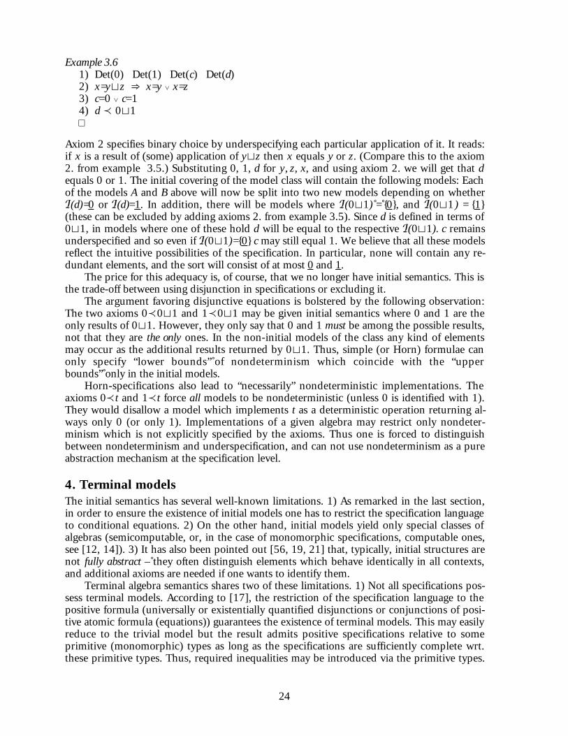
24

Example 3.61) Det(0) Det(1) Det(c) Det(d)2) x=ytz ⇒ x=y ∨ x=z3) c=0 ∨ c=14) d ≺ 0t1¤

Axiom 2 specifies binary choice by underspecifying each particular application of it. It reads:if x is a result of (some) application of ytz then x equals y or z. (Compare this to the axiom2. from example 3.5.) Substituting 0, 1, d for y, z, x, and using axiom 2. we will get that dequals 0 or 1. The initial covering of the model class will contain the following models: Eachof the models A and B above will now be split into two new models depending on whetherI(d)= 0 or I(d)= 1 . In addition, there will be models where I(0t1) = { 0 }, and I(0t1) = { 1 }(these can be excluded by adding axioms 2. from example 3.5). Since d is defined in terms of0t1, in models where one of these hold d will be equal to the respective I(0t1). c remainsunderspecified and so even if I(0t1)={ 0 } c may still equal 1. We believe that all these modelsreflect the intuitive possibilities of the specification. In particular, none will contain any re-dundant elements, and the sort will consist of at most 0 and 1 .

The price for this adequacy is, of course, that we no longer have initial semantics. This isthe trade-off between using disjunction in specifications or excluding it.

The argument favoring disjunctive equations is bolstered by the following observation:The two axioms 0≺0t1 and 1≺0t1 may be given initial semantics where 0 and 1 are theonly results of 0t1. However, they only say that 0 and 1 must be among the possible results,not that they are the only ones. In the non-initial models of the class any kind of elementsmay occur as the additional results returned by 0t1. Thus, simple (or Horn) formulae canonly specify “lower bounds” of nondeterminism which coincide with the “upperbounds” only in the initial models.

Horn-specifications also lead to “necessarily” nondeterministic implementations. Theaxioms 0≺t and 1≺t force all models to be nondeterministic (unless 0 is identified with 1).They would disallow a model which implements t as a deterministic operation returning al-ways only 0 (or only 1). Implementations of a given algebra may restrict only nondeter-minism which is not explicitly specified by the axioms. Thus one is forced to distinguishbetween nondeterminism and underspecification, and can not use nondeterminism as a pureabstraction mechanism at the specification level.

4. Terminal modelsThe initial semantics has several well-known limitations. 1) As remarked in the last section,in order to ensure the existence of initial models one has to restrict the specification languageto conditional equations. 2) On the other hand, initial models yield only special classes ofalgebras (semicomputable, or, in the case of monomorphic specifications, computable ones,see [12, 14]). 3) It has also been pointed out [56, 19, 21] that, typically, initial structures arenot fully abstract – they often distinguish elements which behave identically in all contexts,and additional axioms are needed if one wants to identify them.

Terminal algebra semantics shares two of these limitations. 1) Not all specifications pos-sess terminal models. According to [17], the restriction of the specification language to thepositive formula (universally or existentially quantified disjunctions or conjunctions of posi-tive atomic formula (equations)) guarantees the existence of terminal models. This may easilyreduce to the trivial model but the result admits positive specifications relative to someprimitive (monomorphic) types as long as the specifications are sufficiently complete wrt.these primitive types. Thus, required inequalities may be introduced via the primitive types.

25

2) Furthermore, the data types obtained by terminal semantics are co-semicomputable [12,14].

An advantage of the terminal models is that they do not distinguish elements which areobservationally equivalent. Every other model M can be seen as a refinement – an imple-mentation – of the terminal model Z, and the unique homomorphism M→Z serves as thenatural abstraction function which determines the equivalence on the concrete representa-tions of the abstract values. Focusing on observational equivalence, terminal models are oftenwell suited for studying implementation relations.

These properties are carried over to the terminal models of nondeterminate specifica-tions. While constructing initial power set models of nondeterminism poses severe problems,one has at least obtained a characterization of the congruence determining the terminal mul-timodel. Let B be a multimodel of a specification SP, and L(B) be the class of multimodels ofSP such that for every M∈L(B) there exists a (loose) multihomomorphism M→B.

Theorem 4.1 [53]. A multimodel B is terminal in the class (L(B),MHom) iff it identi-fies all consistent values.¤

Thus, recalling the definition of consistency from 2.17, a terminal model has to identify twovalues whenever there is a possibility that they may give rise to the same observations in allcontexts.

The theorem is qualified by the clause “B is terminal in L(B)” which means that we stilldo not have the criteria for the existence of terminal models. In particular, the work in [53]has a purely semantic character and no formal specification language is considered. We may,however, use the theorem to show that a terminal model does not exist for a specification SPby showing that the class of multimodels of SP, MMod(SP), is not equal to the class L(B) forany model B which identifies all consistent values.

In [21] terminal semantics is used to study the implementation relation between fourkinds of nondeterminism. The programming languages CN, BN, AN, and LN are specifiedwhich include, respectively, erratic, demonic, angelic, and loose nondeterminism (which,roughly, reflects the idea of a specification with loose deterministic semantics). For the defi-nition of these notions a predicate “loops” is introduced which expresses the possibility ofnontermination (loops(s)=F iff s always terminates). The terms correspond to the statements ofthe intended programming language, and the models of the specifications represent the pos-sible semantics of the languages. It is shown that the first three, CN, AN, and BN, have ter-minal models. These are of special interest because they are

1. minimally defined, i.e., whenever there is a semantics in which some statement sis undefined, then this possibility is reflected in the terminal model where s isundefined too, and

2. fully abstract, i.e., two statements which have the same loops values and thesame result sets are equal.

LN does not have a terminal model, but all minimal models of LN are possible deterministicsemantics of LN and are possible implementations of some of the terminal models of CN, ANor BN. The implementation ordering ≤I on models is defined in the natural way [93, 53, 18]:

M ≤I N iff for all terms t, elements a:loops(tN)=F ⇒ loops(tM)=F aM ∈ {tM} ⇒ aN ∈ {tN}

That is, M implements N if it terminates at least in the situations when N terminates and isnot more nondeterministic than N. The result states then that the terminal models for ANand BN are incomparable but both are possible implementations of the terminal model of

26

CN. This reflects exactly our intuition about the relation between these forms of nondeter-minism. Erratic nondeterminism (CN) is the most general and both angelic (AN) and de-monic (BN) ones are possible specializations. Angelic and demonic nondeterminisms are, ofcourse, mutually exclusive – neither subsumes the other. Finally, any nondeterminate opera-tion which does not require fairness may be implemented (loosely) by a deterministic opera-tion.

We may look at this result as a semantic counterpart of the complexity analysis of non-deterministic computations from [25]. Different kinds of nondeterminism are there classifiedaccording to the complexity of their loops predicate. Unbounded erratic nondeterminism isthe most complex class which can be fully characterized only by ( 1

1 formulae, while angelicnondeterminism (bounded as well as unbounded) requires only P 1

0 formulae. Of course, thedeterministic programs are simplest in this respect – they do not require the loops predicate atall since it can be uniquely determined from their input-output relation (which in all cases isof the same, partial recursive complexity, ( 1

0). Other, more specific forms of biased nonde-terministic computations are also included in the classification in [25].

The reader is referred also to [19, 20] for more details about the general approach onwhich the results from [21] are based.

5. Solutions of recursive equations – continuous models.One of the reasons for the great importance of the initial models is that they, in a sense,“represent” the whole class of models. In particular, equality on the ground terms in an initialmodel “represents” the equality on such terms in all models. In order to check whether aground equation holds in some model A we can check whether it holds in the initial one, andif it does conclude that it holds in A. Equations of a specification define the operations whichare legal interpretations of the operation symbols. In particular, recursive equations defineoperations – namely operations which, when substituted for the operation symbols in theequations, provide a solution to the equational system. The next natural question is: can suchsolutions be constructed effectively?

The theory of the deterministic languages and specifications knows the “Mezei-Wright-like results” (after [88]) of the form: there is a (symbolic, initial) structure W such that:

1. solving a system of recursive equations over W and interpreting the solution inanother structure A, and

2. interpreting the system in A and solving it directlygive the same result. One of the main results of this kind for the equational specifications isgiven in [40] for W the initial continuous model.

We will summarize briefly the ideas of such a construction and some difficulties in ex-tending it to the nondeterministic case. The issue is especially relevant because it focuses onthe problems of nontermination, finite observability and computability and allows us toidentify some connections between the algebraic and the denotational approaches to seman-tics.

5.1. Deterministic preliminariesLet ( be a determinate signature. Any term t∈W(,X can be considered a tree t ^ reflecting itssyntactic structure. A term defined by recursion may be considered as a, potentially infinite,tree obtained by the stepwise unfolding of the term along its defining equations. An addi-tional symbol ⊥ is used to indicate the “unfinished” unfolding.

Example 5.1Define

f(0) = 0 f(x+1) = f(x)+2

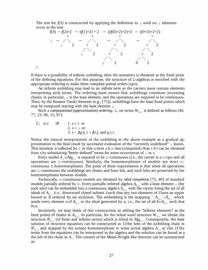
27

The tree for f(3) is constructed by applying the definition to ⊥ until no ⊥ elementsoccur in the tree:

f(3) → f(2)+2 → (f(1)+2) + 2 → ((f(0)+2)+2)+2 → ((0+2)+2+2)+ + + +

⊥ → Á Â → Á Â → Á Â → Á Â⊥ 2 + 2 + 2 + 2

Á Â Á Â Á Â⊥ 2 + 2 + 2

Á Â Á Â⊥ 2 0 2

¤

If there is a possibility of infinite unfolding, then the semantics is obtained as the fixed pointof the defining equations. For this purpose, the structure of (-algebras is enriched with theappropriate ordering to make them complete partial orders (cpo).

An infinite unfolding may lead to an infinite term so the carriers must contain elementsinterpreting such terms. The ordering must ensure that unfoldings constitute increasingchains: in particular, ⊥ is the least element, and the operations are required to be continuous.Then, by the Knaster-Tarski theorem (e.g., [75]), unfoldings have the least fixed points whichmay be computed starting with the least element ⊥.

Such a computational (approximation) ordering , v, on terms W(,⊥ is defined as follows [40,77, 23, 96, 15, 97]:

C: svt iff 1. s $ t or2. s $ ⊥ or3. s $ f(pi), t $ f(ri), and pivri

Notice the natural interpretation of the unfolding in the above example as a gradual ap-proximation to the final result by successive evaluation of the “currently undefined” ⊥ leaves.This intuition is reflected by v in that a term s is v-less (computed) than t if t can be obtainedfrom s by substituting “better defined” terms for some occurrences of ⊥ in s.

Every model A⊥∈Alg(,⊥ is required to be v-continuous (i.e., the carrier is a v-cpo and alloperations are v-continuous). Similarly, the homomorphisms of models are strict v-continuous (-homomorphisms. The point of these requirements is that when all operationsare v-continuous the unfoldings are chains and have lub, and such lubs are preserved by thehomomorphisms between models.

Technically, v-continuous models are obtained by ideal completion [75, 40] of standardmodels partially ordered by v. Every partially ordered algebra A(,⊥ with a least element ⊥ (foreach sort) can be embedded into a continuous algebra A ^(,⊥ with the carrier being the set of allideals of A(,⊥ (i.e., downward closed subsets J such that any two elements of J have an upperbound in J) ordered by set inclusion. The embedding is the mapping ^: A(,⊥→A ^(,⊥ whichsends every element a of A(,⊥ to the ideal generated by a, i.e., the set of all b∈A(,⊥ such thatbva.

Intuitively, we may think of this construction as adding the “infinite elements” as thelimit points of chains in A(,⊥. In particular, for the initial word structure W(,⊥ we obtain thestructure W(,⊥ (of finite and infinite terms) which is initial in Alg(,⊥. Consequently, the leastsolution of recursive equations can be constructed as 1) the lubs of the unfolding chain inW ^(,⊥ and mapped by the unique homomorphism to some actual algebra A⊥, or else 2) theterms from the equations can be interpreted in the algebra and the solution can be found as athe lub of the chain in A⊥. The content of the Mezei-Wright-like theorem can be summarizedas:

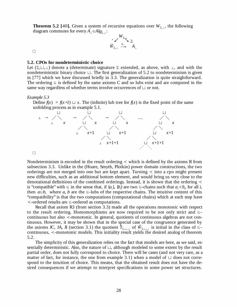
28

Theorem 5.2 [40]. Given a system of recursive equations over W(,⊥, the followingdiagram commutes for every A⊥∈Alg(,⊥:

W(,⊥ ^↙ ↘ 2.

W^(,⊥ 1.→ A⊥

¤

5.2. CPOs for nondeterministic choiceLet ((,t,⊥) denote a (determinate) signature ( extended, as above, with ⊥, and with thenondeterministic binary choice t. The first generalization of 5.2 to nondeterminism is givenin [77] which we have discussed briefly in 3.3. The generalization is quite straightforward.The ordering v is defined by the same axioms C and so lubs exist and are computed in thesame way regardless of whether terms involve occurrences of t or not.

Example 5.3Define f(x) = f(x+1) t x. The (infinite) lub tree for f(x) is the fixed point of the sameunfolding process as in example 5.1.

t t t t⊥ → Á Â → Á Â → Á Â .... Á Â

⊥ x t x t x t x Á Â Á Â Á Â ⊥ x+1 t x+1 t x+1

Á Â Á Â⊥ x+1+1 t x+1+1

N O¤

Nondeterminism is encoded in the result ordering ≺ which is defined by the axioms R fromsubsection 3.3. Unlike in the (Hoare, Smyth, Plotkin) power domain constructions, the twoorderings are not merged into one but are kept apart. Turning ≺ into a cpo might presentnew difficulties, such as an additional bottom element, and would bring us very close to thedenotational definitions of the combined orderings. Instead, it is shown that the ordering ≺is “compatible” with v in the sense that, if {ai}, {bi} are two v-chains such that ai≺bi, for all i,then avb, where a, b are the v-lubs of the respective chains. The intuitive content of this“compatibility” is that the two computations (computational chains) which at each step have≺-ordered results are v-ordered as computations.

Recall that axiom R3 (from section 3.3) made all the operations monotonic with respectto the result ordering. Homomorphisms are now required to be not only strict and v-continuous but also ≺-monotonic. In general, quotients of continuous algebras are not con-tinuous. However, it may be shown that in the special case of the congruence generated bythe axioms JC, JA, JI (section 3.1) the quotient T(,t,⊥ of W ^(,t,⊥ is initial in the class of v-continuous, ≺-monotonic models. This initiality result yields the desired analog of theorem5.2.

The simplicity of this generalization relies on the fact that models are here, as we said, es-sentially deterministic. Also, the nature of t, although modeled to some extent by the resultpartial order, does not fully correspond to choice. There will be cases (and not very rare, as amatter of fact, for instance, the one from example 3.1) when a model of t does not corre-spond to the intuition of choice. This means, that the obtained result does not have the de-sired consequences if we attempt to interpret specifications in some power set structures.

29

This may be explained by the comparison of the intuitive meaning of the tree t^ when the termt is determinate and when it contains applications of t.

Example 5.4.aLet b: → S, f: S→S, and g: S×S→S be determinate operations, and consider the treesfor the terms

t$f(g(⊥,b)): and s$f(⊥tb):

f f| |

t $ g s^ $ tÁ Â Á Â

⊥ b ⊥ b t represents an incomplete evaluation which requires a substitution of some closedterm for ⊥ in order to represent the unique result of the computation (singular se-mantics is assumed). The intuitive interpretation of s, on the other hand, would saythat the t node represents a branching of the computation which may proceed eithertoward b – in which case we have a complete computation, or toward ⊥ – in whichcase we do not have a one. It would not consider s as a single syntactic tree s butrather as a pair of trees, each representing a possible result of the evaluation of s:

f f s^1 $ | s ^2 $ | ⊥ b¤

In short, the branching of a tree at deterministic terms (such as in t ^) has a different meaningthan the branching at t in s ^. The set interpretation of the latter is quite natural and mostauthors do interpret it this way [82, 97, 23]. Unfortunately, the formalization of this intuitioncauses serious problems.

As the example suggests, we would like to define a mapping, C: W(,t,⊥→P(W ^(,⊥) sendinga (possibly infinite) term t ^ to the set of its result trees, i.e., trees where t has been replacedby the chosen branches, and such that the following diagram commutes:

W ^(,t,⊥ C↙ ↘ CA

P(W ^(,⊥) →I P(A⊥)

Fig. 5.5

where: 1. A⊥ is a continuous (-algebra and P(A⊥) is the power set of its carrier. Notice thatA⊥ is deterministic since t∉ (.

2. I: W ^(,⊥→A⊥ is the interpretation of the determinate terms in A⊥. It is shown in[96] that such a continuous interpretation can be obtained as a unique extensionof the interpretation of finite terms W(,⊥→A⊥.

3. I: P(W ^(,⊥)→P(A⊥) is the pointwise extension of 2. to sets.4. CA is a “direct interpretation” of terms involving t in P(A⊥) which should satisfy:

i) CA(t) = { I(t) } for t∈W ^(,⊥ ii) CA(tts) = CA(t) ∪ CA(s)iii) CA(f(ti)) = { fA(ai) | ai∈CA(ti) }

Equations 4.i-ii) require that CA interprets t as the set of results obtained by performing allchoices in the term, and iii) requires singular semantics of the arguments.

If there exists such a C which is continuous then we can construct the lub in W(,t,⊥, mapit on the set of the result trees in P(W ^(,⊥) and interpret the elements of the latter in A⊥, or,

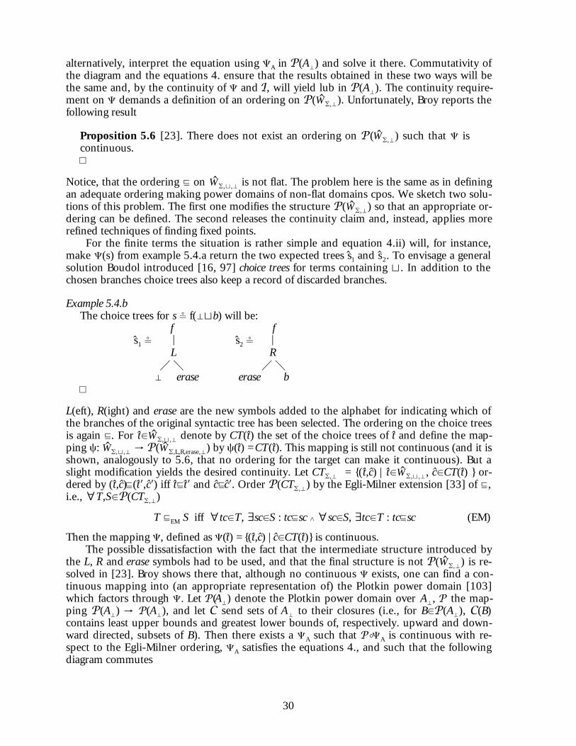
30

alternatively, interpret the equation using CA in P(A⊥) and solve it there. Commutativity ofthe diagram and the equations 4. ensure that the results obtained in these two ways will bethe same and, by the continuity of C and I, will yield lub in P(A⊥). The continuity require-ment on C demands a definition of an ordering on P(W ^(,⊥). Unfortunately, Broy reports thefollowing result

Proposition 5.6 [23]. There does not exist an ordering on P(W ^(,⊥) such that C iscontinuous.¤

Notice, that the ordering v on W ^(,t,⊥ is not flat. The problem here is the same as in definingan adequate ordering making power domains of non-flat domains cpos. We sketch two solu-tions of this problem. The first one modifies the structure P(W ^(,⊥) so that an appropriate or-dering can be defined. The second releases the continuity claim and, instead, applies morerefined techniques of finding fixed points.

For the finite terms the situation is rather simple and equation 4.ii) will, for instance,make C(s) from example 5.4.a return the two expected trees s1 and s ^2. To envisage a generalsolution Boudol introduced [16, 97] choice trees for terms containing t. In addition to thechosen branches choice trees also keep a record of discarded branches.

Example 5.4.bThe choice trees for s $ f(⊥tb) will be:

f fs^1 $ | s^2 $ |

L R Á Â Á Â

⊥ erase erase b¤

L(eft), R(ight) and erase are the new symbols added to the alphabet for indicating which ofthe branches of the original syntactic tree has been selected. The ordering on the choice treesis again v. For t ^∈W ^(,t,⊥ denote by CT(t ^) the set of the choice trees of t ^ and define the map-ping c: W(,t,⊥ → P(W ^(,L,R,erase,⊥) by c(t^) = CT(t ^). This mapping is still not continuous (and it isshown, analogously to 5.6, that no ordering for the target can make it continuous). But aslight modification yields the desired continuity. Let CT(,⊥ = {(t^,c^) | t^∈W ^(,t,⊥, c ^∈CT(t^) } or-dered by (t^,c ^)v(t ^9,c ^9) iff t^vt^9 and c ^vc^9. Order P(CT(,⊥) by the Egli-Milner extension [33] of v,i.e., ∀T,S∈P(CT(,⊥)

T vEM S iff ∀tc∈T, ∃sc∈S : tcvsc ∧ ∀sc∈S, ∃tc∈T : tcvsc (EM)

Then the mapping C, defined as C(t^) = {(t ^,c^) | c^∈CT(t^)} is continuous.The possible dissatisfaction with the fact that the intermediate structure introduced by

the L, R and erase symbols had to be used, and that the final structure is not P(W ^(,⊥) is re-solved in [23]. Broy shows there that, although no continuous C exists, one can find a con-tinuous mapping into (an appropriate representation of) the Plotkin power domain [103]which factors through C. Let P(A⊥) denote the Plotkin power domain over A⊥, P the map-ping P(A⊥) → P(A⊥), and let C send sets of A⊥ to their closures (i.e., for B∈P(A⊥), C(B)contains least upper bounds and greatest lower bounds of, respectively. upward and down-ward directed, subsets of B). Then there exists a CA such that P◦CA is continuous with re-spect to the Egli-Milner ordering, CA satisfies the equations 4., and such that the followingdiagram commutes

31

W ^(,t,⊥ C↙ ↘ CA

P(W ^(,⊥) I Co → P(A⊥)

P ↓ ↓ P

P(W ^(,⊥) I Co → P(A⊥)

Fig. 5.7

Commutativity of the upper triangle of this diagram is the required Mezei-Wright-like result.One can interpret a term t^∈W ^(,t,⊥, using CA, directly in P(A⊥) as a set of the elements of A⊥or interpret t ^ as a set of trees over W ^(,⊥ which are then interpreted in A⊥. Notice that all setsin the image of CA (and C) are closed. This extends the notion of finite observability – if allfinite approximations of an element s are in the set CA(t^) then so will s.

The construction of CA involves finding fixed points in P(A), S(A) (the Smyth powerdomain [117]) and taking the minimal function approximating the former and approximatedby the latter. For the details of this construction, we refer the reader to [22, 23]. An exten-sive, both introductory and advanced, material on the power domains and continuity of thenondeterministic choice can be found in [106, 110, 118, 5, 99, 105, 3, 31, 18, 48].

The discussion above was concerned with singular (IO) semantics only. Detailed com-parison of the Mezei-Wright-like results for IO vs. OI algebras can be found in [34, 35].

6. Reasoning SystemsAs the variety of the proposals discussed so far indicates, the semantics of nondeterminism iscertainly not a closed research topic. This is perhaps one of the reasons why relatively littlework focuses on the reasoning about nondeterminism. Initially, one attempted to reducesuch reasoning to reasoning about some deterministic equivalents. These attempts are thetopic of 6.1. Only very recently some authors began to design systems for direct reasoningabout nondeterminism. We give an example of such a system in 6.2. The following section 7discusses the reasoning systems based on rewriting.

6.1. Reduction to determinismThe early approaches attempted to effect a reduction of the nondeterministic axioms to thesemantically equivalent deterministic ones and to apply the standard forms of reasoning tothe latter. In [121] such a translation is given for a specification language with equality inter-preted as set equality. In order to specify nondeterministic operations one also allows charac-teristic predicates describing the result sets. These predicates, although a part of the specifica-tion, are not, strictly speaking, a part of the specification language. (They are similar to the“semantic functions” loops and elem from [21], or breadth from [18].)

Example 6.1Binary nondeterministic choice

t: Nat×Nat→Natcan be specified with the help of the predicate

Pt: Nat×Nat×Nat→BoolPt(x,y,z) is to be true iff z is a possible result of xty. So we define:

Pt(x,y,z) = (x=z ∨ y=z)¤

32

The problem of reasoning with the nondeterminate terms arises because they do not have thesubstitutivity property. Variables refer to the elements of the semantic domain while nonde-terminate terms denote sets of such elements. The characteristic predicate specification aboveis reasonable only because the variables x, y, z refer to single values and not sets (or arbitraryterms). Thus the substitution of xty for z, although consistent with the signature and syn-tactically correct, is not really meaningful since it yields

Pt(x,y,xty) = (x=xty ∨ y=xty)which would make choice return always the first or always the second argument. In a sense,the predicates are at a different syntactic level of the specification than the (nondeterminate)terms. The formulae one reasons about are equations, and predicates are used only to makethe following translation into the first order language possible.

Let us consider the equation:xty = ytx (a)

Equality is interpreted as set equality, so the translated determinate formula will be:

∀z1:[Pt(x,y,z1) ⇒ ∃z2:(Pt(y,x,z2) ∧ z1=z2)] ∧ ∀z2:[Pt(y,x,z2) ⇒ ∃z1:(Pt(x,y,z1) ∧ z1=z2)] (a9)

It would be rather annoying to write the general translation pattern for equality, but theabove example illustrates the point. It says: (a) holds iff for every possible result z1 returnedby xty there exists a result z2 returned by ytx such that z1=z2 and vice versa.

“Elementwise” reasoning can then be carried out in full first order logic. Denote the re-sult of translating an equation e by FOL(e) (for First Order Logic). All equational axioms e ofthe specification are translated into FOL(e) and a formula a is valid iff FOL(a) follows fromthe derived axioms. One can save some work by avoiding translation of deterministic termsand carrying them directly to the derived formulae. However, it is in general undecidablewhether a given nondeterminate term is deterministic or not [18], so such an improvementwould be limited to a syntactic check on the occurrences of nondeterminate subterms.

FOL will leave all logical symbols except for = unaffected, e.g., FOL(¬e) = ¬FOL(e),FOL(e1∨e2) = FOL(e1)∨FOL(e2), etc. Using this observation, [64] generalizes FOL to conditionalequations. Let b be a Boolean expression in the specification language (not a characteristicpredicate), e an equation. The translation of b ⇒ e is defined as FOL(b=T) ⇒ FOL(e). For in-stance, take b to be 0 < 0t1, and consider the conditional formula:

0 < 0t1 ⇒ e (b)

It will be translated as

[ ∀z:( Pt(0,1,z) ⇒ 0<z ) ∧ ∃z:0<z ] ⇒ FOL(e) (b9)

All nondeterminate subexpressions of b are replaced with new variables (0<z) and these arebound in the characteristic predicates (Pt(0,1,z)) to be the results of the corresponding op-erations. Then the condition of (b9) is true if b holds for all possible results of its nondeter-ministic subexpressions (and there exists a value making b true – this, apparently superflu-ous, conjunct is obtained automatically by applying FOL to b=T). The consequent is just thetranslation of the consequent of (b).

Since 0≮0 the antecedent of (b9) is false and so (b) will be considered true. This may benot quite what we intended when writing (b) since we could have been interested in makinge hold only in the cases when 0t1 returns 1. The translation enforces a uniform interpreta-tion of Boolean expressions – they are either true or false but not indeterminate. This reflectsa general assumption made in [64] that Boolean expressions are, at most, weakly nondeter-ministic – for any argument (a single value) they can be evaluated nondeterministically but

33

their result must be uniquely determined by the arguments. For instance, a Boolean opera-tion b(x) defined as 0<x would be legal, but the one defined as 0t1<x would not. The re-striction is motivated by the fact that Boolean expressions are used there for handling excep-tions, but it also indicates the limitations of the approach.

6.2. Calculus of nondeterminate termsIt is far from pleasing that starting with an equational specification, and being interested onlyin its equational consequences, one has to apply full first order logic. But it seems that thecomplexity of the equational logic of nondeterminism exceeds by far the complexity of theclassical equational reasoning. Other systems which can deal with nondeterminism, espe-cially variants of modal logics (temporal logic [83, 10, 71], dynamic logic [47, 36, 46]), arebased on conceptual models which are much more complex than one would expect, andwish, for a logic of simple specifications with equations/inclusions.

An elegant contribution is that of unified algebras which, being based exclusively onHorn clauses, offer the possibility of taking the full advantage of the existing tools for rea-soning about Horn specifications. The idea, however obvious, is only implicit in the presen-tation of unified algebras – the framework is based on the notion of institutions and deliber-ately abstracts from the peculiarities of the reasoning systems which might possibly be cou-pled with it.

As mentioned before, the main problem with nondeterminate terms is that they cannotbe freely substituted for the (singular) variables. This introduces highly non-standard featuresinto logics of nondeterminism. The only, to our knowledge, calculus for direct reasoningabout nondeterminism which has been shown complete wrt. the multialgebraic semantics isgiven in [127, 126]. The calculus, NEQ, can be used for reasoning about disjunctive clauseswhere each clause C in NEQ is a set of atomic formulae (i.e., the ordering and multiplicity ofthe atomic formulae do not matter), written as e1, ..., en. A clause is interpreted as the dis-junction of its literals.

The atomic formulae e in NEQ are inclusions (s≺t), equalities (sÉt), and inequalities(tºs). Equalities are understood to mean necessary equality (i.e. the two terms always returnthe same result). ` sÉt means not only that t and s are equal but also that they are determi-nistic, and ` tÉt holds only for the deterministic terms. (Thus it is element equality and thesymbol “É” is used instead of “=” to emphasize the distinction w.r.t. standard equality). Ine-qualities are understood to mean necessary inequality (i.e. the two terms never return thesame results). Variables are singular and a clause C is satisfied iff the formula ∀xi(e1∨...∨em) issatisfied, where xi are all variables in C. Equations and inclusions are called positive atoms,and inequations negative atoms. The latter act as negations of both equalities and inclusions.(A slightly different language where the negation of equality does not coincide with the nega-tion of inclusion is used in [130].) For instance, a clause { tºs, p≺r } is thought of as the(equivalent) conditional formula ¬(tºs) ⇒ p≺r, stating that p is included in r whenever t in-tersects s. A clause with exactly one positive atom is a Horn formula, and Horn formulae withno negative atoms are simple formula.

The introduction of inequalities is motivated by the need of binding the applications ofnondeterministic operations, and thus distinguishing between the terms treated as sets andthe results of particular applications of terms corresponding to individuals. A formula` 0t1=0, 0t1=1 says that 0t1 is a set which is either equal to 0 or to 1, in other words,0t1 is not nondeterministic, merely underspecified. In order to express nondeterminism,one has to indicate that not the set but an arbitrary application of (element of the set) 0t1equals 0 or 1. This is expressed by the binding:

` xº(0t1), xÉ0, xÉ1. (6.2)

34

(I.e., for any value x, x is either one of 0 and 1, or it is not a possible result of 0t1.) Thinkingof terms as sets, an inequality ` …sºt.…is a short form for ` ….z∈s, z∈t.…, where z is anew variable, and the inequation in (6.2) corresponds requiring x∈0t1 in the rest of theclause. The two inclusions ` 1≺0t1 and ` 0≺0t1 have the expected multialgebraicmeaning which, together with the above disjunction, will force 0t1 to be interpreted in allmodels exactly as the set {0,1}. Horn-formulae are a special case of clauses and the obviousrestriction of the calculus below can be applied to this case. The rules of the calculus are asfollows :

R1: a) ` xºy, xÉy b) ` xºt, x≺t x, y∈V

R2:`C t

x ; `D, sÉt

`C sx , D

R3: `C t

x ; `D, spt

`C sx , D

x not in a right-hand side of ≺ in C

R4:`C,s¹t ; `D,sºt

`C , D(CUT) (¹ being either É or ≺)

R5:`C

`C,e(WEAK)

R6:

``C x t

C tx

, º(ELIM) x∈V–V[t], at most one x in C

Uppercase Latin letters C, D, denote single clauses and lowercase Latin letters a, e atomicformulae. Semicolon indicates a conjunction of clauses. E.g., if C is {c1, ..., cn}, D is {d1, ...,dm}, and a is an atomic formula, then “C ; D” denotes the conjunction of the two clauses,while “C, D” denotes the clause {c1, …, cn, d1, …, dm}. Similarly, “C, a” is the clause {c1, ..., cn,a} and “C ; a” is the conjunction of C and {a}. C t

x denotes C with t substituted for x.A few comments regarding the rules may be in order.

R1 expresses the relation between º and equality and inclusion. Since variables x and y areindividuals, the two rules correspond to, respectively, x≠y ∨ x=y, and x∉ t ∨ x∈t. They alsoreflect the fact that ‘É’ is a partial equivalence relation and is reflexive only for variables.

R2 is a paramodulation rule allowing replacement of deterministic terms (in the case whensÉt holds in the second assumption). In particular, it allows derivation of the standardsubstitution rule when the substituted terms are deterministic, and prevents substitutionof nondeterministic terms for variables.

R3 allows “specialization” of a clause by substituting for a term t another term s which is in-cluded in t. The restriction that the occurrences of t which are substituted for don’t occurin the right-hand side of ≺ in C is needed to prevent, for instance, the unsound conclu-sion ` p≺s from the premises ` p≺t and ` s≺t.

sºt implies both negation of sÉt and of s≺t. R4 allows us to resolve these complementary at-oms.

R5 allows one to weaken the premise clause by extending it with additional disjuncts.

35

R6 eliminates redundant bindings, namely those that bind an application of a term occurringat most once in the rest of the clause.

The main result concerning this calculus is its soundness and completeness:

Theorem 6.3 [127, 126]. For any specification SP: MMod(SP) ² C iff SP C.¤

The tight relation between multimodels and functional models referred to in proposition 2.6is further strengthened by the fact that the same theorem holds when we replace MMod byFMod.

7. Operational models and rewritingMany authors approach the problem of reasoning about algebraic specifications using someform of rewriting. Rewriting systems have at least two features distinguishing them from thegeneral form of reasoning discussed in this section: 1) they focus on (and are much moreamenable to) automation and 2) they may be also seen as a way of giving the operational se-mantics to the specifications.

Nondeterministic operations have the inherent computational ingredient which determi-nistic functions lack: their result depends on the actual computation since nondeterministicdecisions are made only when the program is executed. The power set constructions modelthis by considering all possibilities in one single model. An operational interpretation, on theother hand, incorporates the fact that nondeterminism is resolved during computation intothe semantic structure.

Such structure is given by a reduction system which simulates the evaluation of terms(programs). Different interpretations of the objects being reduced (as strings, sequences,graphs) and different reduction strategies give rise to a variety of operational semantics.

7.1. Non-confluence and restricted substitutivityThe main idea is to simulate the computation by allowing a nondeterminate term to reduce toany of its possible result. For instance, the reduction rules for the binary choice will be:

xty ½ x and xty ½ y (7.1)

This idea is applied in various operational semantics for the denotational models and l-calculus. In [66, 67] the computation sequences (simulating sequences of nondeterministicchoices), rather than the result sets, are introduced as the basis for a power domain construc-tion. In [70] a similar semantics is shown equivalent to the operational semantics of boundednondeterminism. [5] considers a generalization to unbounded nondeterminism and pointsout that power domains based on the computation sequences help solve the problem of non-continuity of unbounded nondeterministic choice. In [3, 105] noncontinuity is tackled bythe generalization of the semantics of the iterative construct to fixed points over transfiniteordinals (according to the suggestion from [99]), and the resulting Plotkin and Smyth powerdomains for countable nondeterminism are shown equivalent to the respective operationalsemantics. An operational interpretation of l-calculus extended with the choice operator canbe obtained by appropriate modifications of the b-rule. Such modifications, leading to bothplural and singular semantics, are discussed, for instance, in [49, 73, 4]. We will base thefollowing discussion on the terminology of the systems for term rewriting which constitute anatural counterpart to the algebraic specifications.

Since x and y in (7.1) may be arbitrary terms, in particular both may be in normal form(not reducible by the rules of the system) rewriting with nondeterminism will be, typically,non-confluent [24, 59, 57, 97, 4, 87]. One may simply accept it as a fact of life – after all, a

36

nondeterministic computation is precisely one which can return several results, and each re-write represents one among them [59, 4, 87]. Nevertheless, one may try to show some desir-able properties of the resulting system. For instance, in [4] the authors show that their re-writing system is confluent for all terms not involving t, and that for all terms the possiblerewrites constitute exactly the set prescribed by the independently defined model. In thecases when the semantics of a specification is defined also by non-operational means the lat-ter correspondence between the set obtained by all possible rewritings of a term and the setassigned to this term by the static semantics is, of course, an obligation. Inclusion of the for-mer in the latter yields soundness and the opposite inclusion completeness of the reasoningby rewriting.

An exception to the schema (7.1) is the work of Kaplan [63]. It actually forbids rules likethese, except for the one rule of distributivity of t over function application (JD from 3.1oriented from left to right). Instead, terms in normal form may involve t. For instance, onemay define an operation f by the rule f ½ atb. If a and b are irreducible atb will be thenormal form of f. Rewriting is then performed modulo the equations for associativity andcommutativity of t with the rules corresponding to other join axioms (JI and JE from 3.1).This leads to the possibility of obtaining unique normal forms for the nondeterminate terms(bounded nondeterminism) and the conditions for such systems to be confluent are given.An interesting property of such confluent systems is that their initial models are isomorphicto the intuitive multialgebra models with t interpreted as set union.

One of the issues raised by virtually any work on rewriting is the distinction between thesingular and the plural semantics of parameter passing [34, 35, 49, 4, 73]. The need to de-cide when the arguments of the terms under evaluation are to be reduced makes this distinc-tion natural, not to say unavoidable. The two evaluation strategies are present already in therewriting of deterministic terms [43, 98]. Most generally, the singular semantics requires thearguments to be evaluated before the enclosing operation call (IO), while the plural onepostpones their evaluation until the enclosing term has been reduced in its entirety (OI). Thisgives the two substitution rules:

f(x) [x/t]IO ½ U { f(s) | s∈t } (IO)

f(x) [x/t]OI ½ f(t) (OI)

We have adopted the rather informal notation f ½ {...} to indicate that f can be rewritten toany element of the set on the RHS of ½, and s∈t to say that s is (one of) the normal forms oft. For instance, let f(x) ½ x+x and t $ 0t1. Evaluation of f(t) under IO requires that we firstfind all the rewrites of 0t1, and will give us f(x)[x/0t1]IO ½ {f(0), f(1)} ½ {0,2}. OI, on theother hand will yield f(x)[x/0t1]OI ½ f(0t1) ½ 0t1+0t1 ½ {0,1,2}.

OI is a much simpler mechanism than IO. The latter requires that the argument t be firstreduced to (some of) its normal forms s before f(t) can be evaluated. Furthermore, all suchnormal forms must be deterministic in order for IO to yield the singular semantics! For if tcan be reduced to a nondeterminate normal form s then f(x)[x/t]IO will be reduced to a set{...,f(s),...} and then to {...,s+s,...}. Thus, having the singular semantics in mind, one must, inaddition to designing an IO rewriting system, make sure that the system, as well as the speci-fication, satisfy some additional conditions. Such conditions are given by Hußmann in [59,58]. The rewriting system must satisfy the condition that any substitution of a term s for avariable x be guarded by the prior proof that s is deterministic, DET(s). The responsibility ofthe specifier is to ensure that all terms do have a deterministic normal form, i.e.:

∀t∈W(∃s∈W( : t ½* s ∧ DET(s) (DET-completeness)

37

where ½* is the transitive closure of ½. One more condition is needed to ensure the singularsemantics. Any (deterministic) result obtained from a term f(t) must be a result obtained bymaking some choices during the evaluation. The rule f(0t1) ½ c does not determine singu-larity of the argument passed to f. If c is to be produced in the singular semantics fromf(0t1) it must be the result of either f(0) or f(1). This requirement, termed DET-additivity, isensured if the specification with the rewriting rules R satisfies two conditions:

1. ∀ l ½ r ∈ R :  l $ f(t1,...,tn) ∧ ∀i . DET(ti)

2. ∀ f(t1,...,tn) :  DET(f(t1,...,tn)) ⇒ DET(ti) (DET-additivity)

Besides the rules with single variable in the LHS, 1. forbids the rules like f(0t1) ½ c and re-quires that one write instead the rules f(0) ½ c and f(1) ½ c. Analogous requirements of leftt-freeness is made in [63]. 2. says that an operation f with the nondeterministic arguments iscapable of returning a set of possible results. This is again the condition analogous to onemade by Kaplan in [63]. Compared with the latter work the system of Hußmann’s [59] ismuch less restrictive since in [63] it is also required that rules be left-linear, i.e., contain nomultiple occurrences of a variable in LHS. The rewriting system of Hußmann is shown to besound and (weakly) ground complete with respect to the model class (MMod,MHom) ofDET-complete and DET-additive specifications. The calculus of section 6.2 is sound andcomplete for specifications without the restrictions to DET-completeness and -additivity.

What makes nondeterministic OI so much simpler than IO is the fact that the models ofthe former are essentially deterministic power algebras. Hence, the variables in OI refer tosets which are just individuals of the carrier. This is succinctly expressed in:

Proposition 7.2 [34]. OI substitution is associative, i.e.:f(..x..y..z..) ([x/t][y/s])[z/p]OI = f(..x..y..z..) [x/t]([y/s][z/p])OI.

¤

A simple example shows that this is not the case for the IO substitutions:

x + y ([y/x][x/0t1]) [x/0t1]IO = x + y [y/0t1] [x/0t1]IO = {0,1,2} ≠x + y [y/x] ([x/0t1][x/0t1])IO = x + x [x/0t1] [x/0t1]IO = x + x [x/0t1]IO = {0,2}

The lack of associativity of IO substitutions is the reason for the complications of the rewrit-ing systems referred to above. The problem does not arise if there is always at most one oc-currence of a variable to be substituted for or if the substituted terms are deterministic.

Proposition 7.3 [34]. If1. there is at most one occurrence of the variable to be substituted for, or2. any substituted term is deterministic then IO substitution is associative.

¤

1. is reflected in the systems requiring linearity, i.e., forbidding multiple occurrences of avariable, which is a very strong restriction ([63], the introductory system in [58]), and 2. inthe systems, like Hußmann’s, which require a proof of determinacy for the substituted terms.(The calculus from subsection 6.2 takes care of both cases: the restriction on the rule R7 cor-responds to 1, and the second premise in rule R2 to 2. In [130, 131] it is also shown that acomplete extension of the calculus to plural arguments requires only the addition of the stan-dard, unrestricted substitution rule for plural variables.)

Of course, one of the main differences between IO and OI strategies concerns, as in de-terministic rewriting, the termination properties. Since the former requires the evaluation of

38

all arguments before the evaluation of a call, it will diverge in many cases in which the latterwill compute a well defined result. One of the numerous variations on the plural/singular vs.OI/IO distinctions is proposed in [4]. It combines the singular semantics of parameter pass-ing with the preferable termination properties of the OI evaluation strategy by means ofsharing. The idea is to bind (share) the arguments and postpone their evaluation until reduc-tion of the term requires a value of the argument (lazy evaluation). The language (of l-expressions, actually, but we stay with our notation) is extended with the binding construct{x/t} which is performed before substitution:

f(x) [x/t]b ½ f(x) {x/t} (1)

The rest of the system takes then care of rewriting f and t as far as possible, e.g.,

if f(x) ½ f9(x) then f(x){x/t} ½ f9(x){x/t}if t ½ t9 then f(x){x/t} ½ f(x){x/t9} (2)

“As far as possible” is defined with the help of the critical set, CR, of a term. CR(t) is emptywhenever t can be rewritten and contains the variable x if further rewriting of t demands x tobe evaluated. The rule

if x∈CR(f(x)) then f(x){x/t} ½ f(x)[x/t] (3)

performs then the usual substitution [x/t] of t for all x in f(x). By the rules (2), t in the mo-ment of such substitution will be in normal form.

7.2. Rewriting LogicA very powerful and general theory of nondeterministic (and concurrent) rewriting calledRewriting Logic was designed by José Meseguer in [87, 86].

As we have seen, purely equational specifications of nondeterminism do not yield intui-tively plausible results: Defining choice by xty=x, and xty=y gives x=y. On the other hand,the definition xty=x ∨ xty=y does not have an initial model. This motivates the use of inclu-sion (3.2–3.4) or rewrite rules as above. The language of rewriting logic extends the equa-tional language by allowing also conditional rewrite rules. Equations may be considered two-way rewrite rules, but the idea is to simplify the exposition by rewriting in equivalenceclasses modulo the congruence induced by the equations and to use rewrite rules for nonde-terministic terms only. The generalization of the rewriting systems for equational theories liesin allowing conditional rules and labeling the rules (we discuss this point in a moment). Arewrite system S is given by a 4-tuple ((, E, L, R) of signature, equations, labels, and rewriterules labeled by L.

Example 7.4.aFor illustration, we will use the following system S for the natural numbers with bi-nary choice(: 0: → Nat

succ: Nat → Nat+: Nat×Nat → Natt: Nat×Nat → Nat

E: 1. 0+x = 0 2. x+y = y+x3. succ(x)+succ(y) = succ(succ(x+y))4. xty = ytx

L: { r1, r2 }R: r1: xty ½ x r2: xty ½ y¤

39

Rewriting logicThe rewriting logic (RL) is the following set of rules ([t] denotes the equivalence class of t un-der the congruence induced by E; ti,si,wi,vi∈W(,X):

RL1. Reflexivity [t] ½ [t]

RL2. Congruence

[ ] [ ]

[ ( )] [ ( )]

t s

f t f si i

i i

½½

RL3. Replacement

[ ] [ ]

[ ( )] [ ( )]

w v

t w s vi i

i i

½½

for each rule r: t(xi) ½ s(xi) in R

RL4. Transitivity [ ] [ ] [ ] [ ]

[ ] [ ]

t t t t

t t1 2 2 3

1 3

½ ½½

This is the whole logic and its simplicity and intuitive appeal call for no further comments.(We have simplified the rule RL3 which, in general, involves conditionals.) Like in the mostsystems discussed above, a proof in RL will produce a possible result of the argument, for in-stance, RL1 and RL3 will give [xty + z] ½ [x+z] (using r1), and [xty + z] ½ [y+z] (usingr2).

The model T S ( X ) A model of a system S is constructed as a category TS(X) with the objects being the equiva-lence classes [t] for t∈W(,X, and the morphisms the equivalence classes of the terms repre-senting proofs in RL. In order to identify appropriate proof terms (and possibly distinguishtwo morphism with the same source and target) the labels of the rules applied are used. Themorphisms are generated using the rules “simulating” the proof rules of RL which, in addi-tion, attach the appropriate label to each morphism:

1. Identities [t]: [t] ½ [t]

2. (-structure

a

ai i i

i i i

t s

f f t f s

: [ ] [ ]

( ) : [ ( )] [ ( )]

½½

3. Replacement

a

ai i i

i i i

w v

r t w s v

: [ ] [ ]

( ) : [ ( )] [ ( )]

½½

for each rule r: t(xi) ½ s(xi) in R

4. Composition a b

a b

:[ ] [ ] :[ ] [ ]

; : [ ] [ ]

t t t t

t t1 2 2 3

1 3

½ ½½

(writing composition from left to right)

A morphism g: [t] ½ [s] corresponds then to a proof (term) which, by applying the rules g,starts with [t] and produces [s]. To make a category out of this one needs to ensure the asso-ciativity of compositions and to make the morphisms [t] into the identities on the objects [t].The following axioms take care of imposing the required properties on the morphisms:

(assoc) for all a, b, g (a;b);g = a;(b;g)(ident) for all a: [t] ½ [s] a;[s] = a and [t];a = a

Some additional axioms make sure that the appropriate morphisms will be identified. Forinstance, axiom 4. makes [0t1] = [1t0], and hence the morphisms r1([0],[1]): [0t1] ½[0], and r2([1],[0]): [0t1] ½ [0] should be identified. In particular, all equations from Eshould be valid in the model category, so for every equational axiom t(x)=s(x) and all a werequire that the morphisms t(a) and s(a) be equal. This will make, for instance, +([0],[x])equal to the identity morphism [x] for all x.

40

Example 7.4.bA small piece of the category TS(X) for S from example 7.4.a is shown below:

ª ª

ª

[1t2]

r2([0],[1])

[0t1]

[2]

[succ(0t1)]

r1([0],[1])

ª[1]

succ(r1([0],[1])) succ(r2([0],[1]))

r2([1],[2])r1([1],[2])

[0]

ª

ª

¤

Note that the object [succ(0t1)] is not the same as [1t2]. This reflects the ability of themodel to distinguish between plural semantics (which is default) from the singular whichwould require the additional distributivity axiom succ(xty) = succ(x)tsucc(y).The last thing is to interpret the (-structure in TS(X). Two final identifications are:

(comp) for all f, ai, bi f(ai;bi) = f(ai);f(bi)(ident) for all f, ti f([ti]) = [f(ti)]

With these equations, every f∈( determines a functor fTS: TS(X)n → TS(X) (where n is thearity of f). For instance, succ will determine the functor which sends every object [ t] to[succ(t)], and every morphism, like r1([0],[1]), to the respective morphism succ(r1([0],[1])).

The category of S -modelsTS(X) is just one among the possible models of S. For a category C to be an S-model it mustsatisfy all the axioms of S. Intuitively this means that

1. for every t=s ∈ E, the functors tC and sC induced in C should be identical,2. for every [t] ½ [s] ∈ R, there must exist a corresponding arrow in C.

Since t and s may involve variables, 2. is formalized as the requirement of the existence of anatural transformation between the respective functors tC and sC. Finally, the notion of amorphism of S-models is defined as an S-functor which preserves the (-structure and thenatural transformations corresponding to each rule of S. This gives a category S-CAT of allmodels of S. One of the central results about these constructions is:

Theorem 7.5 [87]. The functor S-CAT → SET sending an S-model to the set ofits objects has the left adjoint which sends each set X to TS(X).¤

The first thing one obtains from this theorem is an easy proof of completeness of RL with re-spect to S-CAT (of course, RL is also sound for this class). It also suggests a generalized ini-tial semantics for rewrite systems since any system S has now the initial model TS. The list ofvarious approaches which can be subsumed under rewriting logic is quite impressive. Weonly mention the link to the classical initial algebras.

Given a standard rewriting system S one can construct the initial model for S provided itis confluent. The present construction assigns an initial model to any S system – also theones which involve nondeterminism in the form of non-confluent rewrite rules (or are not

41

confluent for other reasons). If S happens to determine an initial algebra TS, or, more gener-ally, if we are interested in the initial model TS of the equational theory corresponding to S ,then TS may be obtained as a quotient of TS. The equational theory for S is the one where all½ have been turned into =. This means that all we have to do is to impose such equalities onthe morphisms (representing ½) in TS. We unlabel all morphisms and make [t]=[s] when-ever there is a morphism [t] ½ [s]. The image of TS under this transformation will be TS. Infact, the transformation is a functor and it will send S-CAT onto the class Mod(S) of ordi-nary (-models of the equational theory of S.

7.3. Reasoning and rewriting with sets.The rewriting relation t½* s, interpreted in the equational case as the equality of t and s, hasbeen redefined for the nondeterministic rewriting to mean that t is possibly equal to s (or thats≺t). As we have seen, an immediate consequence is a lack of confluence. Since ≺ is not anequivalence relation, this poses a more general question of rewriting in the presence of suchrelations. In particular, inclusion is just one among the common set-relations. Thus reasoningabout nondeterminism becomes closely related with reasoning with sets (as observed in[129]) – an area of increasing importance, especially in logic and constraint programming[114, 32, 61, 120]. The suggested extensions go in the direction of rewriting atoms – pairs ofterms annotated with an appropriate relational symbol – rather than rewriting of terms.

The authors of bi-rewriting [72] propose the use of two kinds of relations: ½⊂ and ½⊃ . Toprove t≺s, one will try to rewrite t to a term u replacing it by “bigger” terms along the relation½⊂ . Simultaneously, one tries to rewrite s to u replacing it by “smaller” terms along the rela-tion ½⊃ . Existence of such a u (which need not be unique) proves the inclusion. The use oftwo relations gives more flexibility in applying different simplification orderings because nowthe ordering of terms need not coincide with their inclusions ≺.

A related approach from [69] introduces a language for specifying the relations: ≺, a,and = which, interpreted in multialgebras, correspond to inclusion, intersection and identityof 1-element sets. The associated reasoning is based on the replacement and compositionalproperties of these relations. A sound and refutationally ground-complete system for the lan-guage of sequents over such atomic relations is given. Rewriting is done using the corre-sponding relations: ½⊂, ½⊃ , ½a , and ½= . In particular, in the course of a rewriting proof thepredicates may change according to the laws of their composition, yielding all the time thestrongest possible relation between the active terms. For instance, two rewriting steps t½⊃ sand s½⊂ u will lead to a derivation of t½a u, while the steps t½⊃ s and s½= u will yield t½⊃ u.

The above works extend the equational rewriting generalizing several classical notionssuch as overlapping rules, critical pair, confluence. In particular, the notion of unique normalform becomes less central. Instead, one has to invent a search strategy which finds appropri-ate atoms/terms for chaining proofs (such as the term u in s½⊃ u and t½⊂ u needed to completethe proof of t≺s).

8. SummaryNondeterminism poses many problems which cannot easily be incorporated into the frame-work of deterministic specifications. The formalization of the intuition that nondeterministicoperations generate sets of possible results, reflected in the power set structures, presents se-rious difficulties. The proposed generalizations of the classical results such as those on ini-tiality, continuity, and equational reasoning to the power set structures have only limited va-lidity. The most successful proposals are rather sophisticated and apply to non-standard con-structions. They are often very general, addressing other problems besides that of nondeter-minism.

42

The fundamental difficulty seems to lie in the inherently computational character ofnondeterminism which confronts the attempts to enclose it in a single, preferably initial,model. This difficulty may be expressed by the slogan that “choice is not a constructor.” Anoccurrence of the syntactic operation t in specifications will typically be reflected in the ini-tial model by the occurrence of the respective choice terms, such as atb. They, however,represent a kind of “intuitive junk” because choice is not supposed to introduce any newelements into the model. On the other hand, the intended meaning cannot be covered by thepurely equational language, which corrupts the nature of the choice operator and reduces itto a deterministic function.

The solution comes in some form of the “is a possible result” predicate. It is present inalmost all approaches as inclusion, partial ordering or rewrite rules. In cases when the initialsemantics can be obtained – and these are the cases when the specifications are restricted toHorn theories – such a predicate corresponds to the intuitive meaning of the nondeterminis-tic operations.

For multialgebras, the initial semantics can be obtained only in particular cases. To guar-antee its general applicability one has to introduce some partial order models. Such models,however, are based on blurring the distinction between individuals and sets. In particular,they give the predicate “is a possible result of” a mathematically simpler, but intuitively lessobvious, meaning than the set based models do.

Loose semantics of nondeterminism has not received much attention. The restriction toHorn theories, even with the “is a possible result” predicate, have more undesirable conse-quences for such semantics than in the deterministic case. The general models of determinatespecifications introduce junk (undenotable elements), but the behavior of the operations ap-plied to such elements is still controlled by the axioms. This is no longer the case when wemove to the nondeterministic specifications. The axioms x≺xty and y≺xty specify only thelower bound on the admitted nondeterminism of the choice operator. In the general powerset models, the interpretation of nondeterministic ground terms such as 0t1 will be allowedto return any imaginable (and unimaginable) results besides the two prescribed by such aspecification. Thus junk will appear, so to speak, not only next to non-junk but also in themiddle of it. (This does not apply to the unified algebras where the interpretation of choice asjoin excludes such situations.)

The computational character of nondeterminism finds its natural expression in the op-erational models. At the syntactic level it is reflected in the fact that nondeterminate terms donot denote unique values, and consequently violate the requirements of referential transpar-ency and substitutivity. This leads to an operational approach not only in the semantics, butalso in the reasoning. With the exception of the rewriting logic, this indicates why one had toawait completeness results of the proposed reasoning systems for so long. Also, such systemsusually describe the result set of a term not by a single formula but by a set of formulae – onefor each possible result. Hence, a deduction of the result set of a term requires derivations ofall such formulae. The reasoning must not only consider the syntax of the formulae involvedbut also ensure that all possible rules have been applied. However, this deficiency does notoccur in the calculus from 6.2.

With respect to the last point, as well as to the deficiencies of Horn-specifications, dis-junctive axioms provide significant help. However, such axioms do not admit initial modelsand introduce a few extra complications in the reasoning systems.

An important issue that has not been addressed in this paper concerns the notion of im-plementation of nondeterministic data types. The reason for this omission is the almost com-plete absence of any published results which, we suppose, reflects the absence of active re-search in that area. We may mention two works [107, 132] which both point in the same di-rection: In the context of data refinement it seems necessary to distinguish underspecification

43

from nondeterministic operations by relaxing the referential transparency (unrestricted sub-stitutivity) requirement with respect to the latter. (This relaxation corresponds to the re-stricted substitutivity in the logic discussed in section 6.2.) Mere underspecification excludesthe possibility of verifying implementations which naturally would be considered correct andplausible.

Although there already exists an extensive literature on various aspects of nondeter-minism in an algebraic setting, it does not seem that the research has established some con-sensus similar to the one discernible in the classical specifications of deterministic data types.Such a consensus – concerning not the best and only formalism, but the relative importanceand applicability of different formalisms – is probably needed before the questions about im-plementation and structured specification of nondeterministic data types can receive closerattention.

9. References[1] C. Aarts, R. Backhouse, P. Hoogendijk, E. Voermans, J. Woude, “A Relational Theory

of Datatypes”, 1992, In preparation.

[2] L. Aceto, R. DeNicola, A. Fantechi, “Testing Equivalencies for Event Structures”, inMathematical models for the semantics of parallelism, LNCS, vol. 280, Springer, 1986.

[3] K.R. Apt, G.D. Plotkin, “A Cook’s tour of countable nondeterminism”, in Proceedingsof 8th International Colloquium on Automata, Languages and Programming, LNCS vol.115, Springer, 1981.

[4] E. Astesiano, G. Costa, “Sharing in Nondeterminism”, in Automata, Languages and Pro-gramming, Sixth Colloquium, LNCS, vol. 71, Springer, 1979.

[5] R.J. Back, “Semantics of Unbounded Nondeterminism ”, in Automata, Languages andProgramming, LNCS, vol. 85, Springer, 1980.

[6] R.J.R. Back, J. von Wright, “Duality in Specification Languages: A Lattice-theoreticalApproach”, Acta Informatica, vol. 27, 583-625, 1990.

[7] J.W. de Bakker, “Semantics and Termination of Nondeterministic Recursive Pro-grams”, Automata, Languages and Programming, Edinburgh, 435 - 477, 1976.

[8] F. Bauer, The Munich Project CIP: The Wide Spectrum Language CIP, LNCS vol. 183,Springer, 1985.

[9] H. Bekic, Programming Languages and Their Definition, vol. 177, Springer Verlag, 1984.

[10] M. Ben-Ari, Z. Manna, A. Pnueli, “The temporal logic of branching time”, in Pro-ceedings of Eighth Annual Symposium on Principles of Programming Languages, 1981.

[11] J.A. Bergstra, J.W. Klop, An Abstraction Mechanism for Process Algebras, Tech. Rep. IW231/83, Dept. of CS, Mathematisch Centrum, Amsterdam, 1983.

[12] J.A. Bergstra, J.V. Tucker, “Initial and final algebra semantics for data type specifica-tions”, SIAM Journal on Computing, vol. 12, 366-387, 1983.

[13] J.A. Bergstra, J.W. Klop, “Algebra of communicating processes”, Proceedings of CWISymposium on Mathematics and CS, 89 - 138, Oct. 6-7 1986.

[14] J.A. Bergstra, J.V. Tucker, “Algebraic specifications of computable and semicompu-table data types”, Theoretical Computer Science, vol. 50, 137-181, 1987.

44

[15] S.L. Bloom, R. Tindell, “Compatible orderings on the metric theory of trees”, SIAM J.Comput., vol. 9, no. 4, 683-691, November 1980.

[16] G. Boudol, Calculus maximaux et semantique operationnelle des programmes non deter-ministes, Ph.D. thesis, University of Paris, 1980.

[17] M. Broy, W. Dosch, H. Parsch, P. Pepper, M. Wirsing, “Existential quantifiers in ab-stract data types”, in Automata, Languages and Programming, Sixth Colloquium , LNCS,vol. 71, Springer, 1979.

[18] M. Broy, R. Gnatz, M. Wirsing, “Semantics of Nondeterministic and NoncontinuousConstructs”, LNCS, vol. 69, Springer, 1980, pp. 553 - 392.

[19] M. Broy, M. Wirsing, Initial versus Terminal Algebra Semantics for Partially Defined Ab-stract Types, Tech. Rep. TUM-I 8018, Technische Universität München, December1980.

[20] M. Broy, M. Wirsing, “Programming Languages as Abstract Data Types”, Lille Colloque80, 1980.

[21] M. Broy, M. Wirsing, “On the Algebraic Specification of Nondeterministic Program-ming Languages ”, in CAAP'81, LNCS, vol. 112, Springer, 1981, pp. 162 - 179.

[22] M. Broy, “Fixed point theory for communication and concurrency”, in IFIP TC2Working Conference on Formal Description of Programming Concepts II, North-Holland,1983, pp. 125-147.

[23] M. Broy, “On the Herbrand Kleene universe for nondeterministic computations”, inProc. MFCS’84, LNCS, vol. 176, Springer, 1984.

[24] M. Broy, “A Theory for Nondeterminism, Parallelism, Communication and Concur-rency”, TCS, vol. 45, 1986.

[25] A.K. Chandra, “Computable Nondeterministic Functions”, 19th Annual Symposium onFoundations of Comp.Sci., 1978.

[26] W. Clinger, “Nondeterministic call by need is neither lazy nor by name”, Proc. ACMSymp. LISP and Functional Programming, 226-234, 1982.

[27] P.M. Cohn, Universal Algebra, Mathematics and Its Applications vol. 6, D.Reidel Pub-lishing Company, 1965.

[28] O.J. Dahl, Verifiable Programming, Prentice Hall, 1992.

[29] E.W. Dijkstra, “Guarded Commands, Nondeterminacy and Formal Derivation of Pro-grams”, CACM, vol. 18, 1975.

[30] E.W. Dijkstra, A Discipline of Programming, Prentice-Hall, 1976.

[31] E.W. Dijkstra, “A simple fix-point argument without the restriction to continuity”, inControl Flow and Data Flow, Comp. and System Sciences, Springer, 1984.

[32] A. Dovier, E. Omodeo, E. Pontelli, G.F. Rossi, “Embedding Finite Sets in a Logic Pro-gramming Language”, LNAI, vol. 660, Springer, 1993, pp. 150-167.

[33] H. Egli, A mathematical model for nondeterministic computations, ETH, 1975.

[34] J. Engelfriet, E.M. Schmidt, “IO and OI. 1”, Journal of Computer and System Sciences,vol. 15, 328-353, 1977.

45

[35] J. Engelfriet, E.M. Schmidt, “IO and OI. 2”, Journal of Computer and System Sciences,vol. 16, 67-99, 1978.

[36] Y.A. Feldman, D. Harel, “A probabilistic dynamic logic”, in Proceedings of FourteenthAnnual ACM Symposium on Theory of Computing , 1982.

[37] J.A. Fernández, J. Minker, “Bottom-Up Evaluation of Hierarchical Disjunctive De-dutcive Databases”, Logic Programming, Proc. of the Eight Int. Conf., 1991.

[38] R.W. Floyd, “Nondeterministic algorithms”, Journal of the ACM, vol. 14, no. 4, 1967.

[39] R.J. van Glabbeek, Bounded nondeterminism and the approximation induction principle inprocess algebra, Tech. Rep. CS-R8634, Centrum voor Wiskunde en Informatica, Am-sterdam, 1986.

[40] J.A. Goguen, J. Thatcher, E. Wagner, J. Wright, “Initial algebra semantics and con-tinuous algebras”, Journal Assoc. Comp. Mach., vol. 24, 68 - 95, 1977.

[41] J.A. Goguen, R.M. Burstall, “Introducing Institutions”, in Logics of Programs, LNCS,vol. 164, Springer, 1983.

[42] J.A. Goguen, What is unification? A categorical view of substitution, equation, and solution,Tech. Rep. CSLI-88-124, Center for Study of Languages and Information, 1988.

[43] I. Guessarian, Algebraic Semantics, LNCS vol. 99, Springer, 1981.

[44] J.V. Guttag, The Specification and Application to Programming of ADT, Tech. Rep. CSR6-59, Computer Systems Research Group, University of Toronto, 1975.

[45] G.E. Hansoul, “A subdirect decomposition theorem for multialgebras”, Algebra Uni-versalis, vol. 16, 275-281, 1983.

[46] D. Harel, A.R. Meyer, V.R. Pratt, “Computability and Completeness in Logics of Pro-grams”, in Proceedings of 9th Annual ACM Symposium on Theory of Computing, 1977.

[47] D. Harel, V.R. Pratt, “Nondeterminism in Logics of Programs”, in Proceedings of 5thAnnual ACM Symposium on Principles of Programming Languages, 1978.

[48] R. Heckmann, “Power Domains Supporting Recursion and Failure”, in CAAP’92,LNCS, vol. 581, Springer, 1992.

[49] M.C.B. Hennessy, “The semantics of call-by-value and call-by-name in a nondeter-ministic environment”, SIAM J. Comput., vol. 9, no. 1, 1980.

[50] M. Hennessy, R. Milner, “On Observing Nondeterminism and Concurrency”, inAutomata, Languages and Programming, LNCS, vol. 85, Springer, 1980.

[51] M. Hennessy, “Powerdomains and nondeterministic recursive functions”, in Proc. 5thInternational Symp. on Programming, LNCS, vol. 137, Springer, 1982.

[52] M. Hennessy, “Observing Processes”, in Linear Time, Branching Time and Partial Orderin Logics and Models for Concurrency, LNCS, vol. 354, Springer, 1988.

[53] W.H. Hesselink, “A Mathematical Approach to Nondeterminism in Data Types”,ACM: Transactions on Programming Languages and Systems, vol. 10, 1988.

[54] C.A.R. Hoare, Communicating Sequential Processes, Prentice-Hall International Ltd.,1985.

[55] P.F. Hoogendik, “Relational programming laws in Boom hierarchy of types”, in Pro-ceedings of Mathematics of Program Construction, Springer, 1992.

46

[56] G. Hornung, P. Raulefs, “Terminal algebra semantics and retractions for abstract datatypes”, in Automata, Languages and Programming, LNCS, vol. 85, Springer, 1980.

[57] H. Hußmann, “Nondeterministic algebraic specifications and nonconfluent term re-writing”, in Algebraic and Logic Programming, LNCS, vol. 343, Springer, 1988.

[58] H. Hußmann, Nondeterministic Algebraic Specifications, Ph.D. thesis, Fakultät fürMathematik und Informatik, Universität Passau, 1990.

[59] H. Hußmann, Nondeterminism in Algebraic Specifications and Algebraic Programs, Birk-häuser, 1993.

[60] G. Huet, J. Hullot, “Proofs by Induction in Equational Theories with Constructors”,JCSS, vol. 25, 239-266, 1981.

[61] B. Jayaraman, “Implementation of Subset-Equational Programs”, Journal of Logic Pro-gramming, vol. 12, no. 4, 299-324, 1992.

[62] S. Kaplan, “Conditional Rewriting”, in Conditional Term Rewriting Systems, LNCS, vol.308, Springer, 1987.

[63] S. Kaplan, “Rewriting with a Nondeterministic Choice Operator”, Theoretical ComputerScience, vol. 56, 37-57, 1988.

[64] D. Kapur, Towards a theory of abstract data types, Ph.D. thesis, Laboratory for CS, MIT,1980.

[65] J.R. Kennaway, C.A.R. Hoare, “A theory of nondeterminism”, in Automata, Languagesand Programming, LNCS, vol. 85, Springer, 1980.

[66] P.R. Kosinski, “A Straightforward Denotational Semantics for Non-Determinate DataFlow Programs”, 5th Annual Symposium on PoPL, 1978.

[67] P.R. Kosinski, Denotational Semantics of Determinate and Non-Determinate Data FlowPrograms, Ph.D. thesis, MIT Laboratory of Computer Science, 1979.

[68] D. Kozen, “Semantics of probabilistic programs”, J. Comput. Sys. Sci., vol. 22, 1981.

[69] V. Kriauciukas, M. Walicki, Reasoning and Rewriting with Set-Relations I: Ground Case,CSL’94 [also Tech. Rep. 92, University of Bergen, Dept. of Informatics, 1994.]

[70] R. Kuiper, An operational semantics for bounded nondeterminism equivalent to a denota-tional one., Tech. Rep. IW 169/81, Stichtig Mathematisch Centrum, Dept. of CS, Am-sterdam, 1981.

[71] D. Lehmann, S. Shelah, “Reasoning with Time and Chance”, in Automata, Languagesand Programming, LNCS, vol. 154, Springer, 1983.

[72] J. Levy, J. Augusti, “Bi-rewriting, a term rewriting technique for monotonic order re-lations”, in RTA’93, LNCS, vol. 690, Springer Verlag, 1993, pp. 17-31.

[73] U. de Liguoro, A. Piperno, “Must pre-order in non-deterministic untyped lambda-calculus”, in CAAP’92, LNCS, vol. 581, Springer, 1992.

[74] R.C. Lyndon, “Properties Preserved under Homomorphism”, Pacific Journal of Mathe-matics, vol. 9, 1959.

[75] B. Möller, “On the Algebraic Specification of Infinite Objects - Ordered and Continu-ous Models of Algebraic Types”, Acta Informatica, vol. 22, 537-578, 1985.

47

[76] B. Mahr, J.A. Makowsky, “Characterizing specification languages which admit initialsemantics”, in Proc. 8th CAAP, LNCS, vol. 159, Springer, 1983, pp. 300-316.

[77] T.S.E. Maibaum, The Semantics of Nondeterminism, Tech. Rep. CS-77-30, University ofWaterloo, Ontario, Canada, December 1977.

[78] J.A. Makowsky, “Why Horn Formulas Matter in Computer Science”, Journal of Com-puter and System Science, vol. 34, 266-292, 1987.

[79] A.I. Mal’cev, The Metamathematics of Algebraic Systems, Studies in Logic and the Foun-dations of Mathematics vol. 66, North-Holland Publishing Company, 1971.

[80] A.I. Mal’cev, Algebraic Systems, Die Grundlehren der mathematischen Wissenschaften... Springer, 1973.

[81] A. Manes, “Fuzzy Theories”, Journal of Mathematical Analysis and Applications, 1982.

[82] Z. Manna, “The Correctness of Nondeterministic Programs”, Artificial Intelligence, vol.1, 1 - 26, 1970.

[83] Z. Manna, A. Pnueli, The Temporal Logic of Reactive and Concurrent Systems, Springer,1992.

[84] J. McCarthy, “A basis for a mathematical theory of computation”, in Computer Pro-gramming and Formal Systems, North-Holland, 1963.

[85] S. Meldal, “An Abstract Axiomatization of Pointer Types”, in Proceedings of The 22ndAnnual Hawaii International Conference on System Sciences, IEEE Computer SocietyPress, 1989.

[86] J. Meseguer, A Logical Theory of Concurrent Objects, Tech. Rep. SRI-CSL-90-70,SRI International, 1990.

[87] J. Meseguer, “Conditional rewriting logic as a unified model of concurrency”, TCS, no.96, 73-155, 1992.

[88] J. Mezei, J.B. Wright, “Algebraic automata and context-free sets”, Information andControl, vol. 11, 1967.

[89] R. Milner, “Processes: a mathematical model of computing agents”, Proc. Logic Collo-quium, 1973.

[90] R. Milner, Calculi for Communicating Systems, LNCS vol. 92, Springer, 1980.

[91] P.D. Mosses, “Unified Algebras and Institutions”, in Proceedings of LICS’89, FourthAnnual Symposium on Logic in Computer Science, 1989.

[92] P.D. Mosses, “Unified Algebras and Action Semantics”, in STACS‘89, LNCS, vol. 349,Springer, 1989.

[93] T. Nipkow, “Non-deterministic Data Types: Models and Implementations”, Acta In-formatica, vol. 22, 629 - 661, 1986.

[94] T. Nipkow, “Observing nondeterministic data types”, in Recent Trends in Data TypeSpecification, LNCS, vol. 332, Springer, 1987.

[95] T. Nipkow, Behavioural Implementations Concepts for Nondeterministic Data Types,Ph.D. thesis, Dept. of CS, The University of Manchester, 1987.

[96] M. Nivat, “On the interpretation of recursive polyadic program schemes”, SymposiaMathematica, vol. 15, 255-281 1975.

48

[97] M. Nivat, “Nondeterministic programs: an algebraic overview”, in Information Proc-essing ’80, Proc. of the IFJP Congress ’80, North-Holland Publishing Company, 1980.

[98] M. O'Donnell, “Computing in Systems Described by Equations”, LNCS, vol. 58,Springer, 1977.

[99] D. Park, “On the Semantics of Fair Parallellism ”, in Abstract Software Specifications,LNCS, vol. 86, Springer, 1979.

[100] C.A. Petri, Non-sequential processes, Tech. Rep. ISF-77-05, Gesellschaft für Matematikund Datenverarbeitung, Sankt Augustin, 1977.

[101] G. Pickert, “Bemerkungen zum Homomorphie-Begriff”, Mathematische Zeitschrift, vol.53, 1950.

[102] H.E. Pickett, “Homomorphisms and subalgebras of multialgebras”, Pacific Journal ofMathematics, vol. 21, 327-342, 1967.

[103] G. Plotkin, “A power domain construction”, SIAM Jour. Comp., vol. 5, no. 3, 452 -487, 1976.

[104] G. Plotkin, “Dijksrta’s Predicate Transformers and Smyth’s Powerdomains”, in AbstractSoftware Specifications, LNCS, vol. 86, Springer, 1980.

[105] G. Plotkin, K.R. Apt, “Countable Nondeterminism and Random Assignment”, Tech.Rep. University of Edinburgh, 1982.

[106] G. Plotkin, “Domains”, 1983, lecture notes, Dept. of Computer Science, University ofEdinburgh.

[107] X. Qian, A. Goldberg, “Referential Opacity In Nondeterministic Data Refinement”,ACM LoPLaS, vol. 2, no. 1-4, 233-241, 1993.

[108] J.H. Reif, “Logics for probabilistic programming”, in Proceedings of Twelfth ACM Sym-posium on Theory of Computing, 1980.

[109] W. Reisig, Petri Nets. An Introduction, EATCS Monographs on Theoretical ComputerScience vol. 4, Springer, 1985.

[110] H. Søndergaard, P. Sestoft, Non-Determinacy and Its Semantics, Tech. Rep. 86/12,Datalogisk Institut, Københavns Universitet, January 1987.

[111] N. Saheb-Djahromi, Probabilistic CPO's for Nondeterminism, Tech. Rep. CSR-37-79,University of Edinburgh, Dept. of CS, 1979.

[112] D. Sannella, A. Tarlecki, “Specifications in Arbitrary Institutions”, Information andComputation, vol. 76, 165-210, 1988.

[113] R.L. Schwartz, “An axiomatic treatment of ALGOL 68 routines”, in Proceedings ofSixth Colloquium on Automata, Languages and Programming, vol. 71, Springer, 1979.

[114] J. Schwartz, R. Dewar, E. Schonberg, E. Dubinsky, Programming with Sets; An Intro-duction to SETL, Springer, 1986.

[115] D. Scott, “Continuous Lattices”, in Proceedings of 1971 Dalhousie Conference, LNMvol. 274, Springer, 1972.

[116] D. Scott, “Data Types as Lattices”, SIAM Journal of computing, vol. 5, no. 4, 522-587,1976.

[117] M.B. Smyth, “Power domains”, J. of Computer and System Sciences, vol. 16, 1978.

49

[118] M.B. Smyth, “Power Domains and Predicate Transformers: A Topological View”, Tech.Report, University of Edinburgh, no. CSR-126-83, 1983.

[119] E.W. Stark, “Compositional relational semantics for indeterminate dataflow net-works”, in Category Theory and Computer Science, LNCS, vol. 389, Springer, 1989.

[120] F. Stolzenburg, “An Algorithm for General Set Unification”, in Proceedings of Work-shop on Logic Programming with Sets, ICLP’93, 1993.

[121] P.A. Subrahmanyam, “Nondeterminism in Abstract Data Types”, in Automata, Lan-guages and Programming, LNCS, vol. 115, Springer, 1981.

[122] A. Tarlecki, “Free constructions in algebraic institutions”, in Mathematical Foundationof Computer Science ‘84, LNCS, vol. 176, Springer, 1984.

[123] E. Voermans, “Pers as types, inductive types and types with laws”, in Proceedings ofPHOENIX Seminar and Workshop on Declarative Programming, Springer, 1991.

[124] H. Volger, The Semantics of Disjunctive Deductive Databases, Tech. Rep. MIP-8931,Fakultät für Mathematik und Informatik, Universität Passau, October 1989.

[125] H. Volger, “The semantics of disjunctive deductive databases”, in CSL’89, LNCS, vol.440, Springer, 1989.

[126] M. Walicki, S. Meldal, “A Complete Calculus for the Multialgebraic and FunctionalSemantics of Nondeterminism”, 1993, [to appear in ACM TOPLAS].

[127] M. Walicki, Algebraic Specifications of Nondeterminism, Ph.D. thesis, University of Ber-gen, Department of Informatics, 1993.

[128] M. Walicki, S. Meldal, “Initiality+Nondeterminism => Junk”, Proc. of NIK'93, 1993.

[129] M. Walicki, S. Meldal, “Sets and Nondeterminism”, in Proceedings of Workshop onLogic Programming with Sets: ICLP’93, 1993.

[130] M. Walicki, S. Meldal, “Multialgebras, Power Algebras and Complete Calculi of Iden-tities and Inclusions”, [to appear in Recent Trends in Data Type Specifications, LNCS1995.]

[131] M. Walicki, Singular and Plural Nondeterministic Parameters: Multialgebras, Power Alge-bras and Complete Reasoning Systems, Tech. Rep. 96, Institutt for Informatikk, Univer-sitetet i Bergen, 1994.

[132] M. Walicki, M. Broy, Structured Specifications and Implementation of NondeterministicData Types, Tech. Rep. Technische Universität München, Institut für Informatik,1995.

[133] M. Walicki, S. Meldal, “ Generated Models and the Omega-rule; the NondeterministicCase”, in Proceedings of TAPSOFT'95, 1995.

[134] G. Winskel, “Event structure semantics of CCS and related languages”, in ICALP’82,LNCS, vol. 140, Springer, 1982.

[135] G. Winskel, Event structures, LNCS vol. 255, Springer, 1987.

[136] G. Winskel, “An introduction to event structures”, LNCS, vol. 354, Springer, 1988.

[137] U. Wolter, M. Löwe, “Beyond Conditional Equations”, in CAAP’92, LNCS, vol. 581,Springer, 1992.

50