Non-Urbanised Areas in a metropolitan context. A method for the characterization of agricultural and green infrastructure. Santi Daniele La Rosa Università degli Studi di Catania

Dottorato in Analisi, Pianificazione e Gestione integrate del territorio - XXIV ciclo

Tutor: Prof. Francesco Martinico

2

3

Introduction - Urbanization process and peri-urban spaces in contemporary metropolitan areas

1. Non-Urbanised Areas: definition and role for ecosystem services provision in metropolitan regions 1.1. A definition of Non-Urbanised Areas (NUAs) 1.2. Ecosystem services provided by NUAs 1.3. Overview of urban ecosystem services 1.4. The value of ecosystem services 1.5. Pressures on urban contexts

1.5.1. Urban sprawl 1.5.2. Climate Changes

1.6. Why a characterization of NUAs?

2. Geographic technologies, Planning Support Systems and urban planning 2.1. Rationality and role of information for land-use planning 2.2. Planning and GIS 2.3. Planning Support Systems 2.4. Use of PSS by urban planners

3. Approaches for NUAs planning 3.1. Green infrastructure 3.2. Urban ecological networks 3.3. The agricultural and gree infrastructure

4. The case study: Catania Metropolitan Area 4.1. Introduction to urban sprawl and its dynamics 4.2. Municipalities of Mascalucia, Gravina di Catania and Tremestieri Etneo.

4.3. Land Uses

5. Characterization of NUAs for urban planning: methodology and results 5.1. The analytical phases for NUAs characterization 5.2. Land cover analysis

5.2.1. From Land Use to Land Cover 5.2.2. Geographical Sampling for Evapotranspiration assessment 5.2.3. Results

5.3. Fragmentation Analysis and 5.3.1. Indicators of fragmentation 5.3.2. Results

5.4. Proximity to residential uses 5.4.1. definition of proximity 5.4.2. results

5.5. Land-use suitability model application

4

5.6. Compatibility of proposed uses 5.7. An alternative method for Land Cover extraction: the R package RasClass

5.7.1. Background and methodology 5.7.2. Results

6. Discussions on results, proposals and conclusions

Acknowledgements

References

5

Humanity is

increasingly urban,

but continues

to depend on Nature

for its survival.

6

7

Introduction

Urbanization process and peri-urban spaces in contemporary metropolitan areas

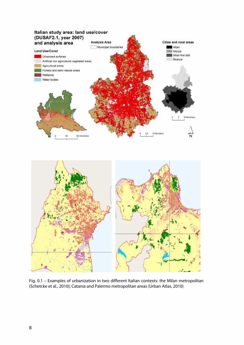
Since decades, in many European countries, dynamics s of urban and economic growth are separated from the demographic development (Kasanko et al., 2006). But despite of the decreasing of population, urban expansion due to spatial development pressure has been an impressive driver of a very high consumption of land and agricultural resources. This has resulted in a overall decreasing of the provision of ecosystem services. In the period between 1990 and 2000, at least 2.8% of Europe´s land had experienced a change in use “including significant increase in urban areas” (Commission of the European Communities 2006). The European Environment Agency (2006) has described the process of the urban sprawl “as the physical pattern of low-density expansion of large urban areas, under market conditions, mainly into the surrounding agricultural areas”. Sprawl is the leading edge of urban growth and implies little planning control of land allocation. Urban development is usually patchy, scattered and strung out, with a tendency for discontinuity. It leap-frogs over areas, leaving agricultural enclaves. Sprawling cities are the opposite of compact cities — full of empty spaces that indicate the inefficiencies in development and highlight the consequences of uncontrolled growth”. In the same document, EEA identified urban sprawl as the “ignored challenge” which urgently demands progressive actions towards sustainable urban development for all the EU-member states. It must be underlined that, although this issue is well known since decades, only recently it has been clearly focused and addressed at the European level, as shown by the important document of (EEA) in 2006. Since the first years of the 70ies, the main Italian cities have started to experience a new model of spatial development that have deeply modified and altered the urban landscape. This process have been called in many different ways, all related to the metropolization of the landscape (Camagni et al., 2002) or the diffuse city (“la città diffusa”, Indovina, 1990). It is present in many Italian metropolitan areas, from the heavily urbanized Milan to the southern metropolitan areas of Catania and Palermo (fig. 0.1). The process of urbanization have changed its pattern. A stronger polarization of services and workplaces toward the CBD of main cities can be observed, but, on the other way, new urbanizations occur on the second or third strip out of the city (Privitera, 2010). Urbanization processes are transferred to agricultural small municipalities close to the main centers, with pressures that these small municipalities are often not able to bear. Urbanizations are not continuous and show low density patterns so that outside the main city the landscape is characterized by a strong degree of fragmentation of agricultural lands and mixes of urban and non-urban uses. An almost endless landscape of low density settlement has became the main landmark of new metropolitan areas. The relationship between the agricultural landscape and the city has produced a particular contemporary peri-urban landscape, where residential low-density settlement are mixed to farmland that have been partially modified and reduced by urbanizations.

8

Fig. 0.1 – Examples of urbanization in two different Italian contexts: the Milan metropolitan (Schetcke et al., 2010); Catania and Palermo metropolitan areas (Urban Atlas, 2010)

9

Today, this peri-urban space is the place where the new urbanizations continue to take place: new fragments of city feature detached or semi-detached houses with small gardens, shopping malls and manufacturing buildings . All these elements keep appearing in the peri-urban areas where agriculture uses can be present or abandoned. More and more people are moving away from the center of metropolitan areas (apparently attracted by the quality of life in these rural settings) to live in residential developments built on converted peri-urban farmlands. “The detached terrace-houses and semidetached houses condense the new type of residential landscape in the metropolitan peripheries of the cities of southern Europe.” (Munoz, 2003). We have seen the born of a new “semi-detached” landscape, “composed, designed and structured as a discontinuous sequence of physical elements: the semi-detached houses themselves, the roundabouts for the distribution of domestic traffic, or the medium and large shopping malls.” (Munoz, 2003). This process of metropolization shows also how settlements belonging to different municipalities, once far one from another, are becoming closer and parts of the same metropolitan area. From a social perspective, the issues concerning the contemporary sprawled models and their impacts are very hard to be communicate to and understood by common people and citizens: for instance the model of detached house is still very idealized and desirable, in a general view that the peri-urban space is as more healthy and pleasant and “ natural” to live in than the urban one. This research of “less urban settlement” or “escape from the city” produces a reverse and contrary effect on the daily behavior of the new city users (Martinotti, 2000) that are forced to spend longer period of their days for moving to/from the main city where workplaces are located. This way of living and moving along the entire metropolitan area is entirely based on the use of private cars, with the related increase of transportation times, costs and environmental externalities. These behaviors are particularly present in metropolitan areas of south Italy, where the development of an efficient public transportation network is still lacking. In contemporary metropolitan areas the concept of rural-urban fringe, as appeared in the geography and planning literature in the 1930s (Whitehand, 1998) ,is today less and less able to distinguish what is urban from it is rural. A chaotic set of land uses is “a product of post-war planning legislation that has partly fossilised some patterns of use, but it is also a reflection of dynamic change as certain components of these areas have grown as part of complex and singular developments (Gant et al., 2011). In new metropolitan contexts, rural land and its agro-ecological features are exposed to dramatic pressures that are driven by the expansion of the urban influence on areas that once were considered as purely rural (Donadieu, 2004).

Impacts on rural and natural areas

In this context, agricultural lands suffer from a wide range of pressures by urbanization process. These pressures are physical, environmental and socio-economical (EEA, 2006). The environmental impacts of sprawl on natural areas are today well documented. Land sustains many ecosystems functions (i.e. production of food, habitat for species, recreation, water retention and storage) that are directly linked with existing land

10

uses. Impacts on natural areas are also exacerbated by the increased proximity and accessibility of urban activities to these areas, that in the past were more far from “urban influence”. This proximity produces stress on ecosystems and species through noise and air pollution. Moreover, the fragmentation caused by transport infrastructures and other urban-related activities creates significant barrier effects that can degrade the ecological functions of natural habitats. Fragmentation can heavily modify corridors spaces for species or can isolate populations by reducing habitats to extent below the minimum area required for the life of these species. Urban development and agriculture compete for the same land, as agricultural lands closer or adjacent to urban areas are ideal places for urban expansion. Farmer’s reasons in this process are clear as they can get substantial financial benefits for the sale of farmland for new housing or other urban developments, especially in times of a general crisis of agriculture. On the other way, agricultural soils need to be conserved, since they are almost non renewable resources. Urban sprawl reduces soils’ capacity to perform their essential functions. Among the main impacts of urban sprawl can be identified the following: soil sealing with a related loss of water permeability, loss of soil biodiversity, reductions of the capacity for the soil to act as a carbon sink are In addition, the rainwater falling on sealed areas presents high levels of pollutants (i.e. high concentrations of heavy metals), being an important threats for the conservation of which the hydrological system. The loss of agricultural land has also major impacts on biodiversity, involving the risk of loosing some valuable biotopes for many species, particularly birds. According to EEA (2006), in Europe the urban expansion tends to “consume the best agricultural lands, displacing agricultural activity to both less productive areas (requiring higher inputs of water and fertilizers) and more remote upland locations (with increased risk of soil erosion). In addition, the quality of the agricultural land that is not urbanised but in the vicinity of sprawling cities has also been reduced”. From a social point of view, sprawl generates can segregation of residential development according to the higher degree of income that are observable in some sprawled settlement, even if this aspect is today not so significant as it was in the past and it is present with less intensity in Italian metropolitan areas. The socio-

economic types of suburban and peripheral areas is characterized by middle and upper income families with children, who have the necessity of a high mobility to let them doing all their daily activities. From an economic perspective urban, sprawl is at the very least a more costly form of urban development due to:

• increased household spending on commuting from home to work over longer distances;

• the cost of the congestion in sprawled areas by inefficient transportation systems;

• the additional costs of the building of new urban infrastructures and related services, across the metropolitan area.

• The reduction of the value of agricultural value of soils with high proximity to urban areas but a complementary increased and related increase of value of the land waiting to be developed

Urban sprawl inhibits the development of public transport and solutions based on the development of mass transportation systems, and the provision of alternative choices in transportation that are essential to ensure the efficient working of urban environments.

11

Numerous studies indicate the increased infrastructure cost associated with sprawl compared with infill or contiguous and compact development (Travisi et al., 2009). These issues may address attempts of control of urban sprawl, by promoting urban policies aimed at the use of public transport and reducing the private car use. Aspects of economic inefficiency are also associated with the market oriented planning that frequently generates sprawled urban areas and has big responsibility in sprawl processes. This kind of market orientates land-use to urban expansion in new areas, without taking into account the potential re-use of former residential or industrial areas. Another important aspect of inefficiency is related to the general savings of energy (consumption of electricity, water, oil and efficiency in waste management), in more compact settlements compared with sprawled one. What’s left?

The process of gradual erosion of peri-urban agricultural land has been accompanied by a low consideration of the important of these areas, often just view as a mere reservoir of space for new urban settlements. Particularly, the agricultural land has been represented in land-use plans during the 70ies and 80ies with different size white patches (“zone bianche”), which strongly characterized the maps of these plans. White as the colour of blank, of places to be filled in with a “built-up anything” or areas waiting for something. During the last 50 years urbanizations, in Italy, peri-urban space has always been considered as an almost unlimited reservoir to be used for new settlement. No consideration about natural resource (soil, water, species, landscape) has been usually attributed to it. Different generations of urban plans have been used soil and agricultural lands as unlimited resources, without any constraint except their geographical extension. In the past, urban planning (strongly driven by real estate market) has not been able to assess agricultural areas in a sufficient way so to recognize the roles, functions and services they provide to human beings. This indifferent towards agricultural peri-urban areas has been one of the reasons at the base of the contemporary sprawling of urbanization process. Since the land has no particular inner value, planners and city decision makers have been moved to use it as a place for new urbanizations without overall landscape project that was able to consider peculiarities and features of peri-urban and agricultural landscape. The new pattern of dispersed, low density development spreads distributes a relevant number of residences (mainly detached and semi-detached houses), retail stores and industrial and office parks across a broad area. Co-existence of developed and agricultural uses in such a settlement pattern is more common than in the homogeneous suburban contexts. For this reason the open spaces between small developments can be utilized for new forms of agriculture (Heimlich and Barnard, 1992). What’s left today of the peri-urban natural agricultural areas? A different mix in types and sizes of residual and Non-Urbanised areas characterize deeply metropolitan landscapes in many Italian regions. Farmland, abandoned or still in use, small orchards, wood and shrubs areas, urban parks, regional parks, reserves and natural protected areas, grasslands (fig. 0.2).

12

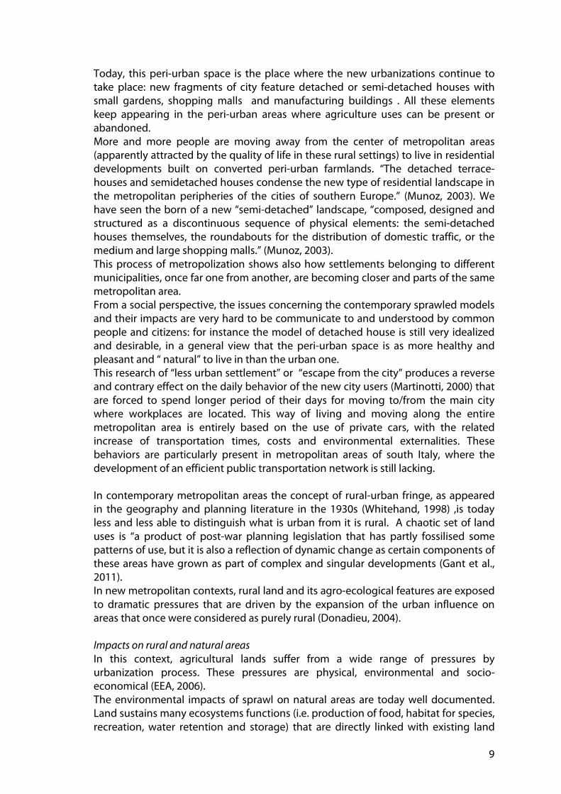
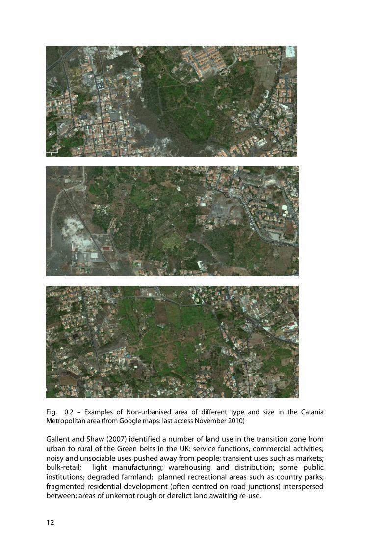
Fig. 0.2 – Examples of Non-urbanised area of different type and size in the Catania Metropolitan area (from Google maps: last access November 2010) Gallent and Shaw (2007) identified a number of land use in the transition zone from urban to rural of the Green belts in the UK: service functions, commercial activities; noisy and unsociable uses pushed away from people; transient uses such as markets; bulk-retail; light manufacturing; warehousing and distribution; some public institutions; degraded farmland; planned recreational areas such as country parks; fragmented residential development (often centred on road junctions) interspersed between; areas of unkempt rough or derelict land awaiting re-use.

13

Despite the very different geographical location, these pattern of land uses are very similar to the ones that can be found in Italian contexts. These areas are characterize by various sizes: this is a common features of these metropolitan contexts, where the very different pattern of urban growth has produced a various range of size and extent of Non-Urbanised areas. Another important common feature of these areas is the high proximity to urban land uses (residential, retails, manufacturing) and this have a lot of consequences from different side like the value of the land or its accessibility. Despite the dramatic urbanization processes, these areas are still present in metropolitan context, still provides important and numerous ecosystem services (see section 1) and therefore need to be accurately analyzed and assessed, in order to develop new scenarios for the land-use of these areas. Moreover, understanding the contemporary Non-Urbanised areas is important for a correct and up to date analysis of the develop of metropolitan contexts and of the complex processes that have define these contexts. The characterization of these areas with appropriate analytical tools is therefore a fundamental step for urban planning to identify their peculiarities and potentialities and to better choose the most appropriate land uses to maintain their integrity and provided ecosystem services.

14

1. Non-Urbanised Areas: definition and role for ecosystem services provision in metropolitan regions

1.1. A definition for Non-Urbanised Areas in metropolitan contexts

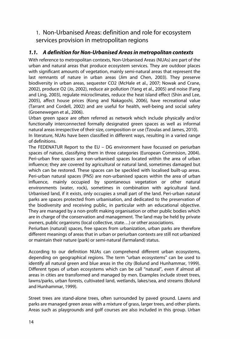
With reference to metropolitan contexts, Non-Urbanised Areas (NUAs) are part of the urban and natural areas that produce ecosystem services. They are outdoor places with significant amounts of vegetation, mainly semi-natural areas that represent the last remnants of nature in urban areas (Jim and Chen, 2003). They preserve biodiversity in urban areas, sequester CO2 (McHale et al., 2007; Nowak and Crane, 2002), produce O2 (Jo, 2002), reduce air pollution (Yang et al., 2005) and noise (Fang and Ling, 2003), regulate microclimates, reduce the heat island effect (Shin and Lee, 2005), affect house prices (Kong and Nakagoshi, 2006), have recreational value (Tarrant and Cordell, 2002) and are useful for health, well-being and social safety (Groenewegen et al., 2006). Urban green space are often referred as network which include physically and/or functionally interconnected formally designated green spaces as well as informal natural areas irrespective of their size, composition or use (Tzoulas and James, 2010). In literature, NUAs have been classified in different ways, resulting in a varied range of definitions. The FEDENATUR Report to the EU – DG environment have focussed on periurban spaces of nature, classifying them in three categories (European Commision, 2004). Peri-urban free spaces are non-urbanised spaces located within the area of urban influence; they are covered by agricultural or natural land, sometimes damaged but which can be restored. These spaces can be speckled with localised built-up areas. Peri-urban natural spaces (PNS) are non-urbanised spaces within the area of urban influence, mainly occupied by spontaneous vegetation or other natural environments (water, rock), sometimes in combination with agricultural land. Urbanised land, if it exists, only occupies a small part of the land. Peri-urban natural parks are spaces protected from urbanisation, and dedicated to the preservation of the biodiversity and receiving public, in particular with an educational objective. They are managed by a non-profit making organisation or other public bodies which are in charge of the conservation and management. The land may be held by private owners, public organisms (local collective, state…) or other associations. Periurban (natural) spaces, free spaces from urbanization, urban parks are therefore different meanings of areas that in urban or periurban contexts are still not urbanized or maintain their nature (park) or semi-natural (farmaland) status. According to our definition NUAs can comprehend different urban ecosystems, depending on geographical regions. The term “urban ecosystems” can be used to identify all natural green and blue areas in the city (Bolund and Hunhammar, 1999). Different types of urban ecosystems which can be call “natural”, even if almost all areas in cities are transformed and managed by men. Examples include street trees, lawns/parks, urban forests, cultivated land, wetlands, lakes/sea, and streams (Bolund and Hunhammar, 1999). Street trees are stand-alone trees, often surrounded by paved ground. Lawns and parks are managed green areas with a mixture of grass, larger trees, and other plants. Areas such as playgrounds and golf courses are also included in this group. Urban

15

forests are less managed areas with a more dense tree stand than parks. Cultivated land and gardens are used for growing various food items. Wetlands consist of various types of marshes and swamps. Lakes/sea includes the open water areas while streams refers to flowing water. Other areas within the city, such as dumps and abandoned backyards, may also contain significant populations of plants and animals. It should be possible, however, to place most urban ecosystems or elements in one of the above mentioned categories. In urban planning, classifications and used typologies of NUAs must be site specific, as well as orientated to the aims of the classification itself. In this research, we will deal with an urban context of the Catania metropolitan area (see section 4), characterized by a considerable presence of urban settlement at different density (from historical centers to sprawled low density settlements). The following category/typologies of NUAs can be found in the study area of the Catania Metropolitan area (see section 4), as mapped by land-use (see section 5). Agricultural areas

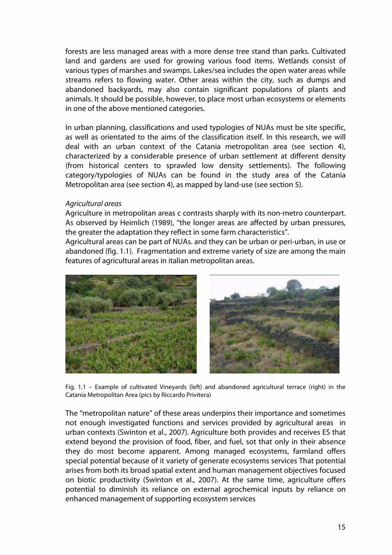
Agriculture in metropolitan areas c contrasts sharply with its non-metro counterpart. As observed by Heimlich (1989), “the longer areas are affected by urban pressures, the greater the adaptation they reflect in some farm characteristics”. Agricultural areas can be part of NUAs. and they can be urban or peri-urban, in use or abandoned (fig. 1.1). Fragmentation and extreme variety of size are among the main features of agricultural areas in italian metropolitan areas.

Fig. 1.1 – Example of cultivated Vineyards (left) and abandoned agricultural terrace (right) in the Catania Metropolitan Area (pics by Riccardo Privitera)

The “metropolitan nature” of these areas underpins their importance and sometimes not enough investigated functions and services provided by agricultural areas in urban contexts (Swinton et al., 2007). Agriculture both provides and receives ES that extend beyond the provision of food, fiber, and fuel, sot that only in their absence they do most become apparent. Among managed ecosystems, farmland offers special potential because of it variety of generate ecosystems services That potential arises from both its broad spatial extent and human management objectives focused on biotic productivity (Swinton et al., 2007). At the same time, agriculture offers potential to diminish its reliance on external agrochemical inputs by reliance on enhanced management of supporting ecosystem services

16

Moreover, we consider also green spaces which are not necessary connected in a network and that can be sprawled and dispersed inside and around the urban system.

Fig. 1.2 - Ecosystem services to and from agriculture (Swinton et al., 2007) Woods

In Catania metropolitan area woods are generally highly fragmented patches among sprawled urban settlements and the mosaic of agricultural areas (Dazzi, 2007). They represent the last remnants of wider natural systems, once present in the area of Mt. Etna, typically represented by oaks woods (Quercus virgiliana, Quercus dalechampii,

Quercus congesta) (fig. 1.3).

17

Fig. 1.3 – Trees and fruit of the Quercus Virgiliana (source: Dipartimento di Botanica dell’Univerisità di Catania: http://www.dipbot.unict.it/ctnatura/flora/bo_celt.html, last access: 29/11/2011) Shrubs and Re-colonized lava fields

Shrubs (fig. 1.4) are typical types of vegetation of the base belt of Mt. Etna anc can be found under volcanic soil from recent eruptions. This thermophile vegetation (“macchia”) has a high density and it is characterized by specie like Euphorbia dendroides (also typical of marine areas). This vegetation also tends to colonizes lava fields (fig. 1.5) or abandoned farmlands and it is usually replaced by steppes of Hyparrhenia hirta, Asphodelus microcarpus, Ferula communis

and Thapsia garganica (Messina and Pavone, no date)

Fig. 1.4 – Example of shrubs in Catania Metropolitan Area (pic by Riccardo Privitera)

Fig. 1.5 – Example of colozination of shrubs on lava fields in Catania Metropolitan Area (pic by Riccardo Privitera)

1.2. Ecosystem services provided by NUAs

As previously introduced, NUAs provide different kind of ecosystem services (ES). These services were firstly defined by a work by Costanza et al. (1997) as ‘‘the benefits human populations derive, directly or indirectly, from ecosystem functions’’. In this important work, authors have identified 17 major categories of ecosystem services (fig. 1.6). A number of these ecological services are not consumed by humans directly, but are needed to sustain the ecosystems themselves. Such indirect services

18

include pollination of plants and nutrient cycling, but the classification is not obvious. Another aspect of ES is that they have different spatial cover and extent: services can be available on the local or global scale according to the issue at hand and to the possibility of transferring them from where it is produced to the city where humans benefit from it. Such a transfer can take place both by man-made transport and by natural means (e.g. atmospheric transport). Easily transferred services with a global scope, like CO2 sequestering, do not necessarily have to be produced close to the source of the problem. Services which are impossible to transfer must, however, be generated close to where they are consumed (e.g. noise reduction). There is a main different from an ecosystem service and ecosystem function, as defined by Escobedo et al. (2011), related to the fact that ES are always related to humans. It is this attribute that distinguishes them from ecosystem functions. Ecosystem functions occur independently from the humans who may benefit from them (Tallis and Polasky, 2009). For example, if a tree intercepts polluted air or water, it performs an ecosystem function; if that function improves local air and water quality then the air and water quality improvement is the ES that benefits human’s health. Escobedo et al. (2011) reviewed some definition of ES that are based on this different between ecosystem function and services. “Brown et al. (2007) define ecosystem services as “the specific results of ecosystem functions that either directly sustain or enhance human life.” Similarly, Fisher et al. (2009) define ecosystem services as aspects of ecosystems utilized actively or passively, directly or indirectly to produce human well-being. Boyd and Banzhaf (2007) and Kroeger and Casey (2007) narrow the definition further by arguing that only components of nature that are directly enjoyed, consumed or used to produce human wellbeing should be counted as final ecosystem services” (Escobedo, 2011).

19

Fig. 1.6 - Ecosystem services as defined by Costanza et al. (1997)

1.3. Overview of urban ecosystem services

Humanity is rapidly urbanizing, and it has been evaluated that by 2030 more than 60% of the world population is expected to live in cities (UN, 1997). But even if humanity is increasingly urban, we are still as dependent on Nature as before. When humanity is considered a part of nature, cities themselves can be regarded as a global network of ecosystems. If compared with true, natural ecosystems, the man-made ones are however immature due to features like their rapid growth and inefficient use of resources such as energy and water (Haughton and Hunter, 1994). Odum (1971) even observes that cities are the ‘‘only parasites in the biosphere’’. But there is also a presence of natural ecosystems within the city limits. The natural urban ecosystems contribute to public health and increase the quality of life of urban citizens, e.g. improve air quality and reduce noise. Most of the problems present in urban areas are locally generated, such as those due to traffic. Often the most effective, and in some cases the only, way to deal with these local problems is through local solutions. In this respect, the urban ecosystems are vital. Other issues

20

are generated more globally, but they heavily influence urban environment: risk related climate changes are the most evident of these issues. In urban areas, Bolund and Hunhammar,(1999) summarized some of the generated services can be highlighted from the set listed by Costanza et al. (1997) (fig. 1.6) air filtering (gas regulation), micro-climate regulation, noise reduction (disturbance regulation), rainwater drainage (water regulation), sewage treatment (waste treatment), and recreational/cultural values. Other services, such as food production and erosion control usually have a less importance in urban areas (fig. 1.7).

Fig. 1.7 -Ecosystem services in urban areas (Bolund and Hunhammar, 1999) Accordingly this taxonomy, it can be highlighted as the different ecosystems are able to provide many services. A brief overview follows. Air cleaning and pollution reduction Air pollution caused by transportation and heating of buildings, among other things, is a major environmental and public health problem in cities. Urban vegetation plays an important role in the environment of cities reducing atmospheric levels of greenhouse gases and PM10 (McHale et al., 2007, [Nowak and Crane, 2002] and [Yang et al., 2005] ). The reduction is primarily caused by vegetation filtering pollution and particulates from the air. Filtering capacity increases with more leaf area, and is thus higher for trees than bushes or grassland (Givoni, 1991). Due to the larger total surface area of needles, coniferous trees have a larger filtering capacity than trees with deciduous leaves However, coniferous trees are sensitive to air pollution and deciduous trees are better at absorbing gases. A mix of species therefore seems to be the best alternative. In general, vegetation is much better than water or open spaces for filtering the air. In particular, urban forests can directly affect air quality in two different ways: 1) by increasing dry deposition and thus removing air pollution from the atmosphere, and 2) by increasing biogenic volatile organic compound (BVOCs) emissions that can act as precursors of secondary air pollutants, though both direct and indirect effects can occur (Escobedo and Nowak, 2011). Even if It is clear that vegetation reduces air pollution, less clear is at what level this can occur, since local situation may produce different results in term of local decrease of pollutants. On the contrary, some disservices characterized urban trees and plants, such as the emission of Volatile Organic Compounds, that can contribute to O3 and particulate matter formation, counteracting the potential beneficial effect of trees in improving air quality in urban areas. Furthermore, urban forests might be responsible of other negative effects including allergenic production (pollen), increased water use and general costs of maintenance (Alonso et al., 2011).

21

Results from McHale et al. (2007) have demonstrated that there are several key decisions that can influence the management of urban trees and forest. It is important to consider that there are other ecosystem services associated with urban trees, and, for this reason, one may be willing to spend more per credit than for other projects dedicated to only reducing atmospheric CO2 concentrations.

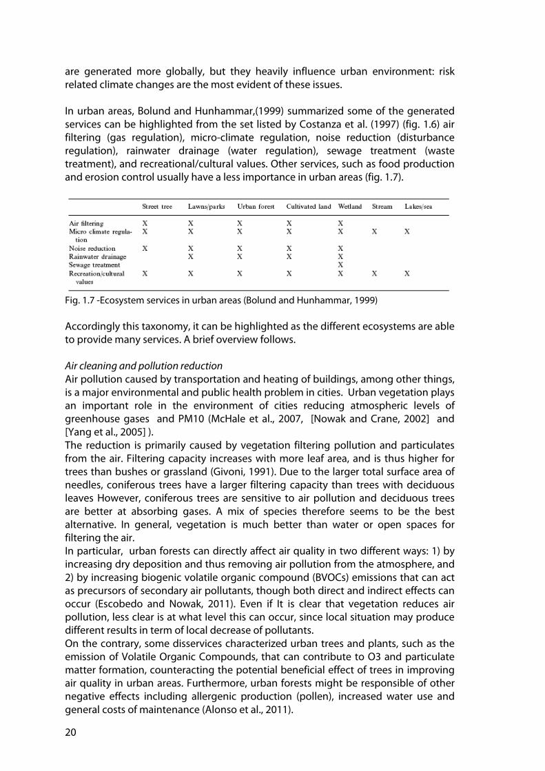
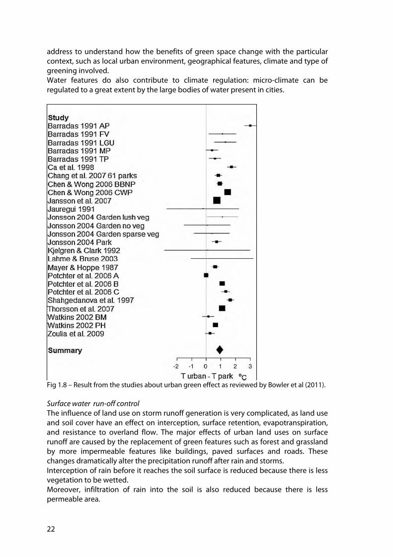
Climate regulation Increased air temperatures can be expected to be particularly problematic in urban areas, where temperatures already tend to be a few degrees warmer than the surrounding countryside. This difference in temperature between urban and rural areas has been called the ‘urban heat island effect’ and it depends on the thermal conductivity and specific heat capacities of materials used in urban areas, surface albedo, the geometry of urban canyons and the input of anthropogenic heat. Urban greening could affect temperatures through different processes (Givoni, 1991; Bowler et al., 2010). A key process is evapotranspiration, which describes the loss of water from a plant as a vapour into the atmosphere. Evapotranspiration consumes energy from solar radiation and increases latent rather than sensible heat, cooling the leaf and the temperature of the air surrounding the leaf. This contrasts with the effect of impervious urban materials such as asphalt and concrete, which do not retain water for evaporation and quickly absorb and retain heat when exposed to solar radiation. In addition to cooling by evapotranspiration, shading from trees can act to cool the atmosphere by simply intercepting solar radiation and preventing the warming of the land surface and air (Oke, 1989). This shading effect may create local cool areas beneath tree canopies and this can be an important issue in the management of urban open spaces. Finally, vegetation may affect air movements and heat exchange. This effect, however, can be expected to be dependent on the type of vegetation. Tree cover may retain warm air beneath the canopy; in contrast, an open grass field that provides low resistance to air flow may promote cooling by convection. A recent overview by Bowler et al. (2010) (fig. 1.8) on different studies about urban greening showed that, on average, an urban park would have around 1 ◦C less than a non-green site. However, this evidence is mostly based on observational data of existing green spaces. Therefore, this hypothesis should continue to be tested through the appropriate monitoring of urban green areas, even if this activity may be often not financial sustainable by local authorities. Monitoring should include collection of temperature data before and after implementation along with comparable ‘control’ non-green sites. Studies that measured temperature from multiple parks in the same urban area presented data showing that larger parks were cooler. Local climate may also affect the temperature of green space but most studies only collected data from a single urban area. The extension of the cooling effect of a green area beyond its boundary is supported by data from a few studies. The scale of any cooling effect beyond the boundary of the green area is particularly important for the likely public health consequences of greening, as green space may not be directly accessible to all who might benefit during very high temperatures. A key line of future research should explicitly investigate the distance and size-dependence of the effects of green areas. Different types of vegetation have shown to have different effects in cooling, particularly depending on the difference between short vegetation, such as shrubs or grass, and more dense tree canopy cover. However, further research should be

22

address to understand how the benefits of green space change with the particular context, such as local urban environment, geographical features, climate and type of greening involved. Water features do also contribute to climate regulation: micro-climate can be regulated to a great extent by the large bodies of water present in cities.

Fig 1.8 – Result from the studies about urban green effect as reviewed by Bowler et al (2011). Surface water run-off control

The influence of land use on storm runoff generation is very complicated, as land use and soil cover have an effect on interception, surface retention, evapotranspiration, and resistance to overland flow. The major effects of urban land uses on surface runoff are caused by the replacement of green features such as forest and grassland by more impermeable features like buildings, paved surfaces and roads. These changes dramatically alter the precipitation runoff after rain and storms. Interception of rain before it reaches the soil surface is reduced because there is less vegetation to be wetted. Moreover, infiltration of rain into the soil is also reduced because there is less permeable area.

23

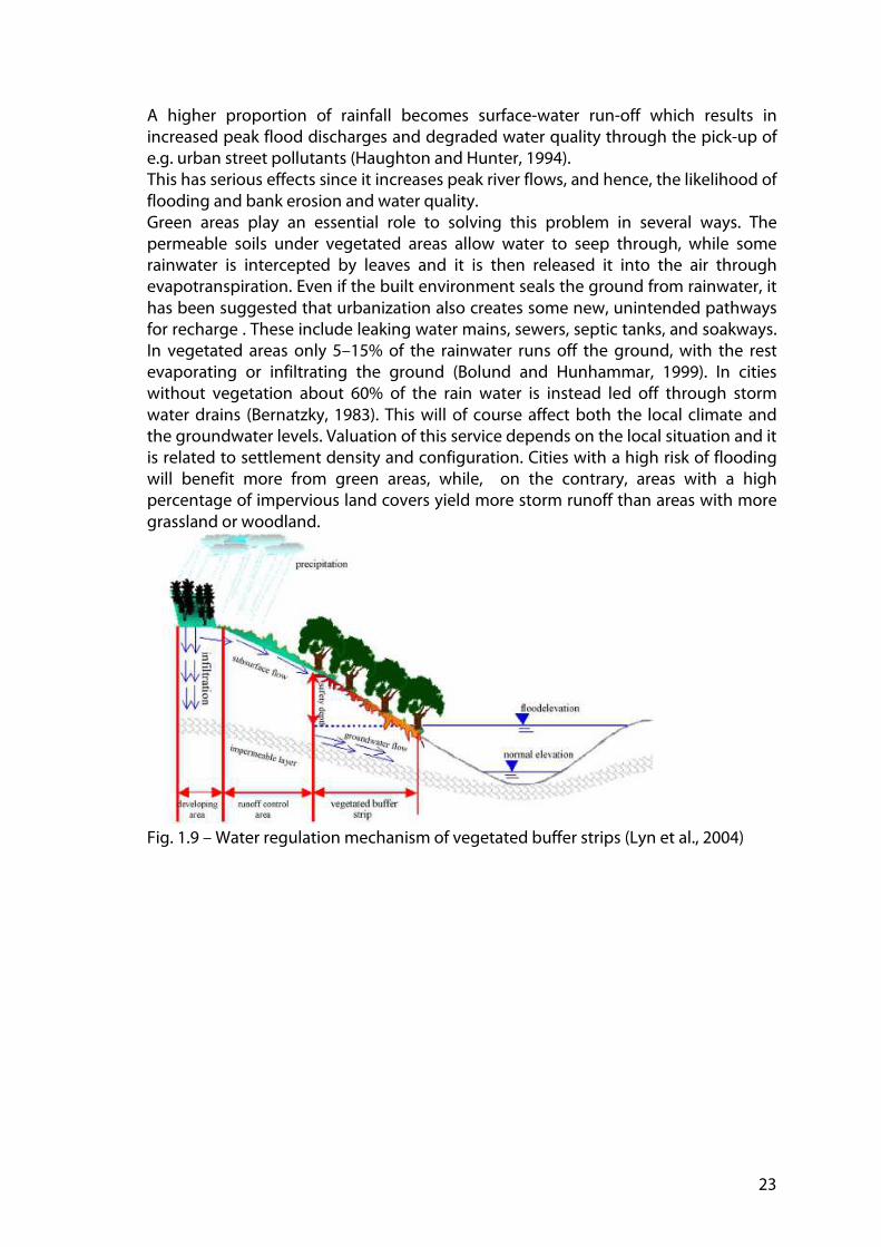
A higher proportion of rainfall becomes surface-water run-off which results in increased peak flood discharges and degraded water quality through the pick-up of e.g. urban street pollutants (Haughton and Hunter, 1994). This has serious effects since it increases peak river flows, and hence, the likelihood of flooding and bank erosion and water quality. Green areas play an essential role to solving this problem in several ways. The permeable soils under vegetated areas allow water to seep through, while some rainwater is intercepted by leaves and it is then released it into the air through evapotranspiration. Even if the built environment seals the ground from rainwater, it has been suggested that urbanization also creates some new, unintended pathways for recharge . These include leaking water mains, sewers, septic tanks, and soakways. In vegetated areas only 5–15% of the rainwater runs off the ground, with the rest evaporating or infiltrating the ground (Bolund and Hunhammar, 1999). In cities without vegetation about 60% of the rain water is instead led off through storm water drains (Bernatzky, 1983). This will of course affect both the local climate and the groundwater levels. Valuation of this service depends on the local situation and it is related to settlement density and configuration. Cities with a high risk of flooding will benefit more from green areas, while, on the contrary, areas with a high percentage of impervious land covers yield more storm runoff than areas with more grassland or woodland.

Fig. 1.9 – Water regulation mechanism of vegetated buffer strips (Lyn et al., 2004)

24

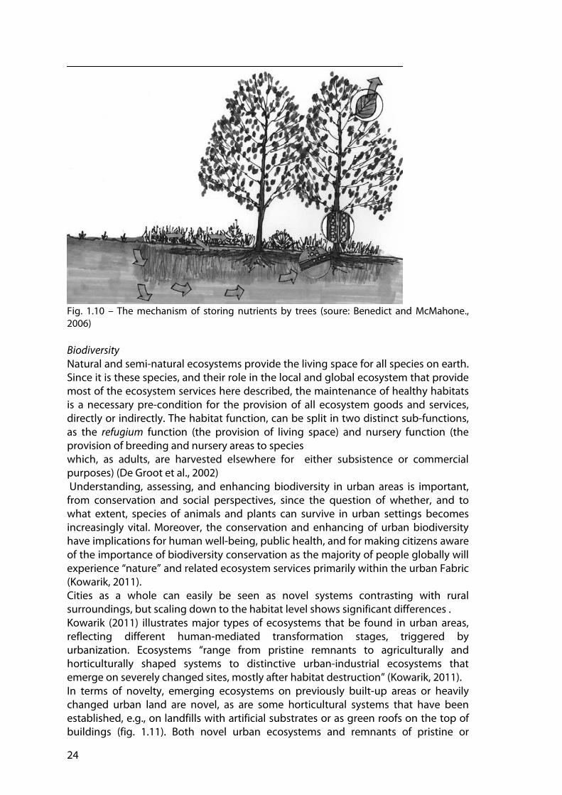
Fig. 1.10 – The mechanism of storing nutrients by trees (soure: Benedict and McMahone., 2006) Biodiversity Natural and semi-natural ecosystems provide the living space for all species on earth. Since it is these species, and their role in the local and global ecosystem that provide most of the ecosystem services here described, the maintenance of healthy habitats is a necessary pre-condition for the provision of all ecosystem goods and services, directly or indirectly. The habitat function, can be split in two distinct sub-functions, as the refugium function (the provision of living space) and nursery function (the provision of breeding and nursery areas to species which, as adults, are harvested elsewhere for either subsistence or commercial purposes) (De Groot et al., 2002) Understanding, assessing, and enhancing biodiversity in urban areas is important, from conservation and social perspectives, since the question of whether, and to what extent, species of animals and plants can survive in urban settings becomes increasingly vital. Moreover, the conservation and enhancing of urban biodiversity have implications for human well-being, public health, and for making citizens aware of the importance of biodiversity conservation as the majority of people globally will experience “nature” and related ecosystem services primarily within the urban Fabric (Kowarik, 2011). Cities as a whole can easily be seen as novel systems contrasting with rural surroundings, but scaling down to the habitat level shows significant differences . Kowarik (2011) illustrates major types of ecosystems that be found in urban areas, reflecting different human-mediated transformation stages, triggered by urbanization. Ecosystems “range from pristine remnants to agriculturally and horticulturally shaped systems to distinctive urban-industrial ecosystems that emerge on severely changed sites, mostly after habitat destruction” (Kowarik, 2011). In terms of novelty, emerging ecosystems on previously built-up areas or heavily changed urban land are novel, as are some horticultural systems that have been established, e.g., on landfills with artificial substrates or as green roofs on the top of buildings (fig. 1.11). Both novel urban ecosystems and remnants of pristine or

25

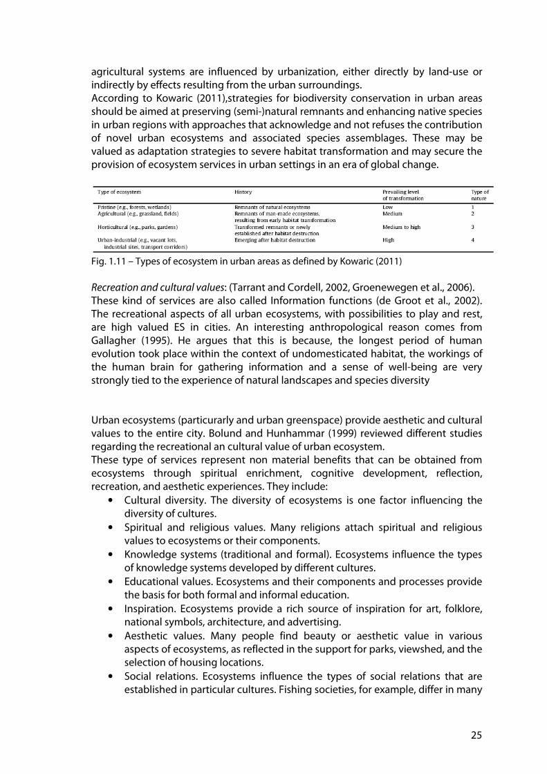
agricultural systems are influenced by urbanization, either directly by land-use or indirectly by effects resulting from the urban surroundings. According to Kowaric (2011),strategies for biodiversity conservation in urban areas should be aimed at preserving (semi-)natural remnants and enhancing native species in urban regions with approaches that acknowledge and not refuses the contribution of novel urban ecosystems and associated species assemblages. These may be valued as adaptation strategies to severe habitat transformation and may secure the provision of ecosystem services in urban settings in an era of global change.

Fig. 1.11 – Types of ecosystem in urban areas as defined by Kowaric (2011) Recreation and cultural values: (Tarrant and Cordell, 2002, Groenewegen et al., 2006). These kind of services are also called Information functions (de Groot et al., 2002). The recreational aspects of all urban ecosystems, with possibilities to play and rest, are high valued ES in cities. An interesting anthropological reason comes from Gallagher (1995). He argues that this is because, the longest period of human evolution took place within the context of undomesticated habitat, the workings of the human brain for gathering information and a sense of well-being are very strongly tied to the experience of natural landscapes and species diversity Urban ecosystems (particurarly and urban greenspace) provide aesthetic and cultural values to the entire city. Bolund and Hunhammar (1999) reviewed different studies regarding the recreational an cultural value of urban ecosystem. These type of services represent non material benefits that can be obtained from ecosystems through spiritual enrichment, cognitive development, reflection, recreation, and aesthetic experiences. They include:

• Cultural diversity. The diversity of ecosystems is one factor influencing the diversity of cultures.

• Spiritual and religious values. Many religions attach spiritual and religious values to ecosystems or their components.

• Knowledge systems (traditional and formal). Ecosystems influence the types of knowledge systems developed by different cultures.

• Educational values. Ecosystems and their components and processes provide the basis for both formal and informal education.

• Inspiration. Ecosystems provide a rich source of inspiration for art, folklore, national symbols, architecture, and advertising.

• Aesthetic values. Many people find beauty or aesthetic value in various aspects of ecosystems, as reflected in the support for parks, viewshed, and the selection of housing locations.

• Social relations. Ecosystems influence the types of social relations that are established in particular cultures. Fishing societies, for example, differ in many

26

respects in their social relations from nomadic herding or agricultural societies.

• Sense of place. Many people value the "sense of place" that is associated with recognized features of their environment.

• Cultural heritage values. Many societies place high value on the maintenance of either historically important landscapes ("cultural landscapes") or culturally significant species.

• Recreation and ecotourism. People often choose where to spend their leisure time based in part on the characteristics of the natural or cultivated landscapes in a particular area.

Fig. 1.12 –Green spaces and playgrounds in urban areas (pics: Daniele La Rosa)

Soil retention and formation

The soil retention function mainly depends on structural aspects such as vegetation cover and roots. Tree roots stabilize the soil and foliage intercepts rainfall thus preventing compaction and erosion of bare soil. Plants growing along shorelines and (submerged) vegetation in near-coastal areas contribute greatly to controlling erosion and facilitating sedimentation. The services provided by this function are very important to maintain agricultural productivity and prevent damage due to soil erosion (both from land slides and dust bowls). Soil is formed through the disintegration and degradation of rocks and gradually becomes fertile through the accretion of animal and plant organic matter and the release of minerals. Soil-formation is a very slow process (Rasio, 1999) and natural soils are generated at a rate of only a few centimeters per century and after erosion. Ecosystem services derived from soil formation relate to the maintenance of crop productivity on farmlands and the integrity and functioning of natural ecosystems.

27

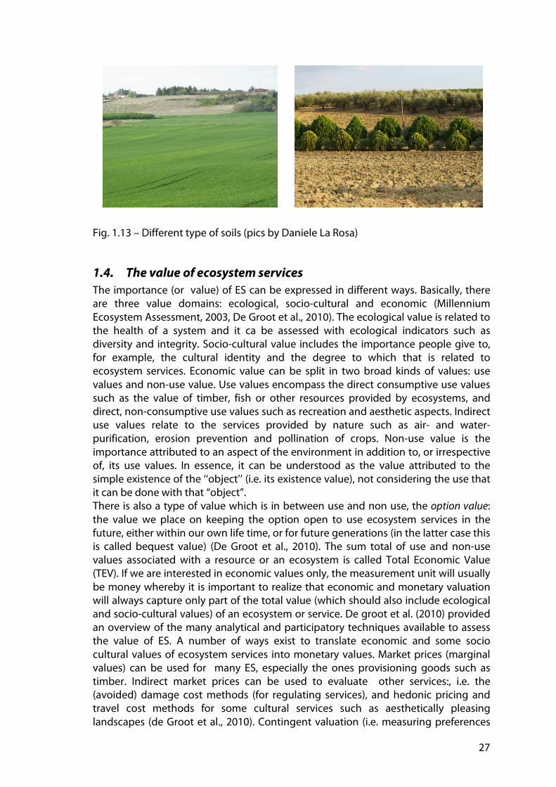
Fig. 1.13 – Different type of soils (pics by Daniele La Rosa)

1.4. The value of ecosystem services

The importance (or value) of ES can be expressed in different ways. Basically, there are three value domains: ecological, socio-cultural and economic (Millennium Ecosystem Assessment, 2003, De Groot et al., 2010). The ecological value is related to the health of a system and it ca be assessed with ecological indicators such as diversity and integrity. Socio-cultural value includes the importance people give to, for example, the cultural identity and the degree to which that is related to ecosystem services. Economic value can be split in two broad kinds of values: use values and non-use value. Use values encompass the direct consumptive use values such as the value of timber, fish or other resources provided by ecosystems, and direct, non-consumptive use values such as recreation and aesthetic aspects. Indirect use values relate to the services provided by nature such as air- and water-purification, erosion prevention and pollination of crops. Non-use value is the importance attributed to an aspect of the environment in addition to, or irrespective of, its use values. In essence, it can be understood as the value attributed to the simple existence of the ‘‘object’’ (i.e. its existence value), not considering the use that it can be done with that “object”. There is also a type of value which is in between use and non use, the option value: the value we place on keeping the option open to use ecosystem services in the future, either within our own life time, or for future generations (in the latter case this is called bequest value) (De Groot et al., 2010). The sum total of use and non-use values associated with a resource or an ecosystem is called Total Economic Value (TEV). If we are interested in economic values only, the measurement unit will usually be money whereby it is important to realize that economic and monetary valuation will always capture only part of the total value (which should also include ecological and socio-cultural values) of an ecosystem or service. De groot et al. (2010) provided an overview of the many analytical and participatory techniques available to assess the value of ES. A number of ways exist to translate economic and some socio cultural values of ecosystem services into monetary values. Market prices (marginal values) can be used for many ES, especially the ones provisioning goods such as timber. Indirect market prices can be used to evaluate other services:, i.e. the (avoided) damage cost methods (for regulating services), and hedonic pricing and travel cost methods for some cultural services such as aesthetically pleasing landscapes (de Groot et al., 2010). Contingent valuation (i.e. measuring preferences

28

based on questionnaires) and benefit transfer (i.e. using data from comparable studies) provide yet other alternatives for evaluation ES. Existing methods have their advantages and disadvantages: although the knowledge base on the monetary value of individual services keep improving, there are still large data gaps and there is still a need for better frameworks, models and data-bases to calculate the TEV of ES.

1.5. Pressures on urban contexts

1.5.1. Urban Sprawl

There is a wide consensus on the idea that sprawl in western countries is heavily affecting the landscape. In Italy, this phenomenon is inexorably wearing down a unique heritage, the result of a long-lasting process of transforming the environment (Settis, 2011). In Italian contexts, sprawl has two main causes. The first is related to the spreading of single-family detached homes, which has become the winning settlement model in many western countries (Bourne, 1996, Peiser, 2001). The result is a continuous loss of agricultural land around the dense network of historical towns that are typical of northern and central regions of Italy (Dematteis, 1997). The second cause is strictly intertwined with the production system of industrial districts (Piccinato, 1993), which is a development model that was particularly efficient for strengthening the country’s competitive edge in the 1990s. At the same time, this model is posing considerable pressure on the environment and landscape, which has been sacrificed due to competitiveness and productivity. Traditional farming settlements have been converted to an endless landscape of small factories mixed with residential subdivisions. The prevailing reason in the examined area is that the diffusion of single-family homes is intertwined with farming. These areas, which can be defined as urbanized countryside, are characterized by many houses, farms and agricultural buildings (Martinico and La Rosa, 2009). The externalities and impacts of sprawl growth patterns on the environment and landscape have been the focus in several studies. The impacts include the following: the loss of fragile environmental lands, increases in air pollution and energy consumption, decreases in the aesthetic appeal of the landscape, the loss or fragmentation of farmland, a reduction in biodiversity, increases in water runoff and risks of flooding, and ecosystem fragmentation (Galster et al., 2001; Johnson, 2001). Loss of agricultural land is often directly connected to land consumption due to sprawl processes (Olson and Lyson, 1999; Thompson and Stalker Prokopy, 2009). There are several consequences to this: landscape fragmentation and simplification, loss of biodiversity, decreasing the agriculture land value, and increasing the externalities of urban sprawl (Johnson, 2001; Camagni, 2002). New urbanizations often occur in proximity to already urbanized areas or existing infrastructure because the price of agricultural land is lower if compared to residential zoned land. Agricultural land usually becomes a highly attractive target for investors and urban developers (EEA, 2006). For these reasons, the hazard of loss of agricultural land may be potentially higher in areas close to already urbanized lands or roads.

1.5.2. Climate changes

Climate changes have been predicted to have many consequences for human health arising from the direct and indirect impacts of changes in temperature and

29

precipitation (McMichael et al., 2003; Patz et al., 2005). One of the primary public health concerns is an increase in the intensity and frequency of heat waves, which have been linked with heat stroke, hyperthermia and increased mortality rates (Tan et al., 2007). For instance, an estimated 15% excess deaths were attributed to dramatic heat waves in Italy in the summer of 2003 (Istituto Superiore di Sanità, no date). Different works show how extreme temperatures area expected more frequently. Annual maximum temperatures will increase more in the centre and south parts of Europe than in the north. A summer increase of temperature will expose Europeans to termic stress with no precedents and this will produce more damages in urban areas. In the Mediterranean area dry period are expected to heavily increase by the end of the century. According to Good et al. (2006) the longest dry period will increase of the 50%, especially in France and Central Europe. These consequences appear to be more dramatic in urban areas, that will be especially vulnerable to the negative aspects of climate change (such as more frequent and severe floods, heat waves, etc.), due to the higher concentration of people and human activities. Urban environments can also be characterized by the combined effects of reduced evapotranspiration (because of less vegetation cover) and the thermal effect off the mass of buildings, which contribute to the heat island effect (Whitford et al., 2001). Urbanization processes lead to changes in the absorption and reflection of solar radiation, and thus the surface energy balance. These changes are dependent from different factors, including the thermal conductivity and specific heat capacities of materials used in urban areas, surface albedo, the shape of urban canyons and the production of heat from human activities (Oke, 1989). Increasing temperatures resulting from global climate change may exacerbate the health impacts of the higher temperatures that are already common in urban areas (Luber and McGeehin, 2008). Thus, there is a pressing need to evaluate strategies that may mitigate against further increases in temperatures in urban areas and the associated negative impacts on human health. An adaptation strategy that has been proposed is to ‘green’ urban areas, essentially by increasing the abundance and cover of vegetation (Givoni, 1991; Gill et al., 2007). Vegetation and urban materials differ in moisture, aerodynamic and thermal properties, and so urban greening could affect temperatures through different processes (Oke, 1989; Givoni, 1991). As previously discussed (see section 1.3) key process is evapotranspiration, which describes the loss of water from a plant as a vapor into the atmosphere. This requires the development of appropriate urban adaptation strategies to mitigate negative impacts of climate changes. As a complement to such adaptation measures, there is a need to ensure that future land-use developments do not worsen the current level of risk, either through influencing the hazards themselves or through affecting the future vulnerability and adaptive capacity of the urban system. Urban planning therefore has a critical role to play, for mitigating the severity of hazards and for reducing the levels of exposure and vulnerability experienced by the urban system. Different scales of planning from macro scale land-use planning to micro scale urban design are both important to this process, responding to the different scales over which risk and vulnerability are expressed (O’Brien et al., 2004). This recognizes that although many aspects of adaptive behavior associated with vulnerability are the result of a decision-making process that operates at an

30

individual level, the government and other policy makers can address this process through their activities. Given the length of time involved in the strategic planning process, and the long lifetime of urban infrastructure, it is even more critical that decision-making does not reinforce negative feedback in any part of the process (Lyndsey et al., 2006). The urgency for information to assist with ‘‘climate conscious’’ planning is evident and ask for detailed tools for the assessment of different urban features that are involved in climate change processes.

1.6. Why a characterization of NUAs?

Concurrent to their role as centers of disturbance, cities are also now home to the majority of humans. This demographic trend in urbanization is more strong in developing countries, but it expects to continue resulting in over 5 billion humans residing in metropolitan centers by the year 2030 (UN, 1997, 2007). As a result, cities have and will increasingly play a key role the delivery of public services as well as offer a critical arena in which to address a wide range of ecosystem health issues. The management of the systems providing ecosystem services becomes important both for the continued delivery of public goods and improving the ecological health of urban areas (Young, 2010). As urban areas are expected to keep growing in the future, planners and political decision makers have to carefully consider the role of NUAs that provide ecosystem services. A better knowledge of the different features of NUAs allows us to identify the more suitable land uses to fulfill the aims of conservation and leisure as well as the promotion of new forms of agriculture (La Greca et al., 2011). Land use planning may allow the protection of green areas that have evapotranspiring and permeable features. This action is directly related to adaptation to climate changes, because it can reduce the urban heat island effect (Bowler et al., 2010) and excessive rainwater runoff. NUAs are also fundamental to increasing urban quality by creating more pedestrian friendly and visually pleasant settlements. Scenarios for land-use should be carefully planned because of the environmental, social, economic and cultural benefits that are derived from the ecosystem services provided by agriculture and green infrastructure. The characterization of NUAs with appropriate analytical tools is therefore a fundamental step to identify their peculiarities and potentialities and to better choose the most appropriate land uses to maintain their integrity and provided ecosystem services. Different models and methodology can be applied in order to help the planning process to better address a new scenario of land uses for these areas.

31

2. Geographic technologies, Planning Support Systems and urban planning

2.1. Rationality and role of information for land-use planning

Urban planning concerns the design and organization of urban physical and socioeconomic space and measures that can be undertaken to solve problems in the use of the land. The general objective is usually to provide decisions about the land-use of activities or urban space which should be better than the existing pattern without planning (Hall 1975). This aim is usually achieved by using knowledge and creativity to design, evaluate and implement a set of justified actions in the public domain (Friedman, 1987). The knowledge may consist of scientific and experiential knowledge, implicit and explicit knowledge, technical knowledge and social knowledge, possessed by a number of societal actors. Geo-information technology developers have long focused on supporting urban planners in handling knowledge and managing considerable amount of information. however There is not a general consensus about the how spatial models and technologies (i.e GIS) for supporting planning and decision making processes. This is partly related to the fact that most planning theories are based on different assumptions regarding rationality. Two types of rationality are of particular relevance for understanding the role of information technology in planning: instrumental (or functional) rationality and communicative (or procedural) rationality (Malczewski, 2004). Instrumental rationality is based on a positivist idea, which puts spatial reasoning (Berry, 1993) and scientific analysis at the core of planning. It assumes a direct relationship between the information available and quality of planning and decision making based on the available information. On the other hand, communicative rationality postulates an open and inclusive planning process, public participation, dialogue, consensus building, and conflict resolution (Innes, 1995). Even if the two perspectives are often viewed as antinomic, the role of information is relevant to both of them. It is rather the way in which the data are processed to obtain information and how this information is used and communicated that make the two perspectives different. The ‘contrast’ between the technological and the political perspectives on the societal implications of geographic technologies is evident in a debate between the techno-positivist (proponents) of GIS and the social scientists (opponents) (Pickles, 1995). Land-use planning is more than a technical procedure, because it also involves participatory approaches. Planners have to deal with different stakeholders, power relationships, and complex urban and regional problems, but they always need considerable amount of spatial information for their activities. This has some important socio-political perspectives on the use of new techniques (i.e. GIS) as tools for planning.

2.2. Planning and GIS

Generally speaking, GIS-based land-use planning should be viewed as a process of converting data to information that adds extra values to the original data. At the

32

subsequent stage of the process, this derived information should be useful to those involved in the planning process. The particular planning needs determine nature and features of the information required. Any planning process must focus on a mix of hard and soft information. Soft data/information is often derived from a public discourse between interest groups and individuals, while hard information comes directly from more codified sources in recognizable formats (cartography, tabular information. …). Central to the land-use planning is the way in which these two types of information are combined and how to define the right balance between the amount of hard and soft information used. The use of soft information may lead to subjective decisions, while, on the other hand, using too much hard information may result in high costs of the analysis phases and in troubles when try to communicate the obtained results. It appears clear that this balance produces a trade-off, that needs to be evaluated on case-by-case basis. GIS have the capabilities of incorporating the soft data in order to be useful in answering questions related to the land-use planning. One can suggest that information systems for planning in general and land-use suitability analysis in particular should be constructed with at least two interrelated perspectives in mind: (i) the techno-positivist perspectives on GIS, and (ii) the sociopolitical, participatory GIS perspectives. Fig. 2.1 illustrates the evolving perspectives of planning and geographic technology, as indicated by Malczeswki (2004). Over the last four decades, the planning paradigm shifted from the applied science approaches in the 1960s through the political process-oriented perspective in the 1970s, and a focus on communication in the 1980s to collective-design approaches in the 90ies (Klosterman, 2001).

Fig. 2.1 . The evolving perspectives of planning and geographic technology,

33

According to the applied science approach, planning is fundamentally a sequence of rational and technical procedures (Hall, 1975). Central to the scientific approach is the instrumental rationality of the positivist paradigm. From this perspective, GIS is seen as a data-centered information technology that provides tools for deriving information from databases to be used in value-free process of rational planning. The underlying assumption—derived from the positivist paradigm—is that there is a direct relationship between the data processing capability and information availability on one hand, and the quality of planning on the other. The better data processing capabilities (and more information), the better is the quality of planning. During the late 1970s and the 1980s there has been an increasing criticism of the applied science model of planning. This criticism was a part of broader critique of positivism. It has been argued that the scientific view of planning is essentially a-historic and it fails to address the relationship between planning and the society that should benefit of the decision of planners. The criticism of the scientific approaches focused on its implicit spatial determinism and the logical impossibility of defining spatial variables that are independent of the context within which they are supposed to operate. A disillusionment with the applied science model of planning led, in the 1970s, to the adoption of a strong political perspective of planning. This perspective recognizes that planning has to deal with socio-political issues that are composed of interest groups with conflicting values and different preferences. According to this perspective, the importance relies on the process of development for the particular societies in which planning is carried out. This approach is referred to as the communicative (substantive or procedural) rationality (Nedovic´-Budic´, 1998). According to Klosterman (2001), planning is ‘an inherently political and social process of interaction, communication, and social design’. Some elements of the planning process may be well defined, but there are significant components of subjective knowledge, common wisdom, etc.. that should be involved in the process.

2.3. Planning Support Systems

The idea of combining the objective and subjective elements of the planning process in a computer based system lies at the core of the concept of Spatial Decision Suppor Systems (SDSS), Spatial Experts Systems (SES), and Planning Support System (PSS). DSS is a computer-based system designed specifically for supporting the user in tackling semi-structured problems and it can be applied in different fields. Although an application of an SDSS for solving a decision making problem may increase the efficiency of the data and information processing operation, this is not the real aim of the system. More important, SDSS aim to improve the effectiveness of decision making by incorporating judgments and results obtained from computer-based algorithms within the decision making process. The system should support a variety of possible decisions that may be present in a particular context for a particular scope. Consequently, the key feature of any SDSS is not to replace a user’s judgments, but to support user in achieving ‘better’ decisions. SDSS provide judgmental information in the form of preferences about the significance of impacts, which cannot be expressed a priori in a formal language. The system should help the users to explore the decision problem in an interactive and recursive fashion. In order to achieve this end, the ability of a GIS to handle judgments involved in the planning process is of critical importance, if the system is to be used as a SDSS. This calls for a representation of the judgments, values, arguments and opinions in the system. One

34

way of doing this is to incorporate decision analytical techniques (e.g. multicriteria analysis), into the GIS-based planning process. Unlike SDSS, SES is based on an assumption that the system can be used by nonexperts to improve their problem-solving capabilities. An SES software can be defined as a computer-based system that employs reasoning methodologies in a particular spatial problem domain in order to transfer expertise and render advice or recommendations, much like a human expert (Laurini, 2001). PSS can be considered as an example of collaborative DSS. The PSS concept has been developed in the context of urban and regional planning (Harris, 1989). They have been defined as a subset of geo-information technologies dedicated to support those involved in planning in exploring, representing, analyzing, visualizing, predicting, prescribing, designing, implementing, monitoring and discussing issues associated with the the planing objective (Batty 1995). PSS combine the functionalities of GIS with models and visualisation. They function as “information frameworks” that integrate the full range of information technologies useful for supporting the specific planning context for which they are designed (Klosterman, 1998; Geertman and Stillwell, 2002). Inventories show that PSS cover a wide range of tools that are readily available for planning support purposes. PSS are systems that have been developed and are being used to support current practice in any public or private sector planning context at any spatial scale. In fact, PSS is a term that refers to the diversity of geotechnology tools, which are primarily developed to support planning processes both in terms of derivation and evaluation of alternative futures. One of the basic assumption in PSS is that an increase in access to relevant information will lead to a greater number of alternative scenarios, and thus a better informed public debate. Well-designed PSS should provide an interactive, integrative, and participatory support for poorly structured planning tasks. It integrates multiple technologies and common interface. Klosterman (2001) suggests that PSS are “an information framework that integrates the full range of current (and future) information technologies useful for planning”. PSS should be organized around the GIS technology, since GIS includes the geographic component which is fundamental in all planning applications. PSS should also incorporate planning tools such as economic and population analysis and forecasting, environmental, land use and transportation modeling. In addition, PSS should include other relevant technologies allowing for handling both quantitative and qualitative data to facilitate public participation and group interaction (Harris, 1989; Bishop, 1999; Klosterman, 2001). Currently, web-based applications are the most relevant among these technologies for their potential of being published and distributed by web-GIS sources like Google maps. With respect to the used knowledge, PSS can be divided into instruments to support the provision of knowledge to those involved in planning, instruments to support communication of knowledge and systems to support knowledge analysis. As reviewed by Carsjens and Ligtenberg (2007), examples of PSS include 3D-visualization tools, land-use modelling tools for urban growth, collaborative planning and decision-making tools, GIS-based multiple criteria evaluation tools and Web-based planning support tools. Recent overviews on the diversity of PSS have been presented by Brail and Klosterman (2001) and Geertman and Stillwell (2002).

35

In many cases, however, it is useful to ask again “Where is the System?” in PSS (Bishop, 1998). The appellation `System' suggests an integration of different things so to constitute a complex or unitary whole. A planning office may indeed have an assemblage of complex data and procedures, but, even today, they seldom form a unitary whole. For this reason, the conceptual ideal for a manager of a complex, spatially diverse environment (such as a city) includes: (1) the data storage, analysis and mapping capabilities of GIS; (2) the availability of support models or procedures that are implemented for a single specific scope; (3) a realistic, real-time, interactive visualization of the impact of decisions. All these components should work together with seamless integration, in order to continuously support and link the final planning decisions with the real world. Current GIS software has substantially evolved to better integrate different geographic data formats, and this has been an important step for the practical need of planners that usually have to cope with data coming from different scientific field, sources and authorities.

2.4. Use of PSS by urban planners

Although planners and designers now have access to much larger volumes of geo-data, the adoption and use of PSS is still far from being widespread and far from being effectively integrated into the planning process (Stillwell et al., 1999). More generally, this limit is linked to the criticism of the role of the technology as a tool for planning and decision-making. This criticism comes from social scientists and it focuses on the supposed uneven social consequences of the GIS technology, questioning its impact on equity, justice, privacy, accuracy, accessibility, and quality of life (Sieber, 2003). It was argued that the advancement of the personal computer speed and the lowering of the costs of desktop GIS software have make GIS more popular but a limited success has been achieved in improving the public’s participation in community-based GIS projects. Today this is less true and participation is being strongly helped and addressed thanks to world wide web platforms for storing and displaying geographic information. Tools like Google mapping services are providing new, real time and widespread access to geographic information. Nevertheless, the use of GIS by planner is still limited on simple spatial queries and production of thematic maps. Progress towards the use of GIS beyond these basic activities to help solving key planning problems through more sophisticated analyses has been very limited (Stillwell et al., 1999). Only a small percentage of planners consider GIS technology as an indispensable tool for performing their job properly. Some explanations for this situation are the diversity of analytical tasks that planners perform, the relatively small market for public sector software, and the cost of developing and supporting commercial software (Geertman and Stillwell, 2002). Despite the fact that the application of GIS within planning practice has increased (Geertman, 2002), current geo-information tools are too complex, too inflexible, incompatible with most planning tasks and technology driven rather than user oriented (Nedovic-Budic, 1998; Geertman and Stillwell, 2002. Nedovic-Budic (1998) has shown that within planning practice, whilst the quality of information generated with GIS technology keeps improving, GIS is consistently underemployed for more sophisticated

36

analytical and modeling exercises, and its impact on planning decisions remains low and relegated to querying data and mapping results. Planners remain, at best skeptical, or at worst antagonistic toward highly systematic and computer-based models (Harris, 1998). For this reason, the percentage of planners who consider their geotechnology as an intrinsic and indispensable tool for their job (as financial experts use their spreadsheet software and as medical specialists use their own technology) is still far too low (Geertman, 2002). Today this approach to technology is still present in some planning fields, even it is moved from a skeptical consideration of new models and tools toward a more general “I-can-accept-but-it’s-not-for-me” behaviors. These kind of planners consider and produce plans with software used for representation purpose only (cad and design software in particular). It is very common, at least in Italy that professional planners do not make use of GIS for their work, so that maps and plans are still produced by cad or image design software. It can be said without exaggeration that, generally, the traditional way to urban planning (in the sense of producing plans) has still not changed since the 80ies. This is particularly true for city plans, where even the basic geographical data (i.e. vectorial technical cartography) are often available in cad format for most Italian regions. One of the reason for this trend may be related to factors such as the “sudden” arrival of GIS technologies in a field (urban planning) that was a traditional land of architect or engineers with their rigid and well defined design tools for the representation of the city. Moreover, during the last 10 years, the gap between geographical information technologies and real planning needs has increased: new features in GIS has been quickly coming out, with only little time to be acquired by planners, due to the very fast renovation of software and tools. This also has to be added to the limited amount of tools that are normally needed by the majority of planners for their work, so that the gap between new technologies and real and daily needs has been increasing. Harvey and Chrisman (1998) argued that like other industrial technologies, GIS is socially constructed via negotiations between various social groups such as developers, practitioners, planners, decision-makers, special interest groups, citizens. Actually, this is not perfectly mirrored by last trends in software updating, which show as software houses have pushed the market irrespectively of the real users’ need. The last 10-15 years have seen a massive develop of new GIS software that was not really needed by everyday users like planners. Some critics can be addressed about an excessive and too fast improvement of programs that came out from software houses. This was anticipated by Klosterman in 1998, who suggested that tools for planning were no more developed than they were ten years before. He also hypothesized that the adoption of new tools and the development of computer applications in planning for the next 25 years would have remained disappointing. A recent work by Vonk and Geertman (2008) has focused on the reasons and bottlenecks of the use of PSS in urban planning. According to these authors, despite the many promising characteristics of PSS, this technology is stuck in a vicious circle (Fig. 2.2) caused by a mismatch existing between supply of and demand for PSS. They state that, even in the late 2000ies, PSS have not yet become a wide and common planning practice and that few lessons are actually being learned about the

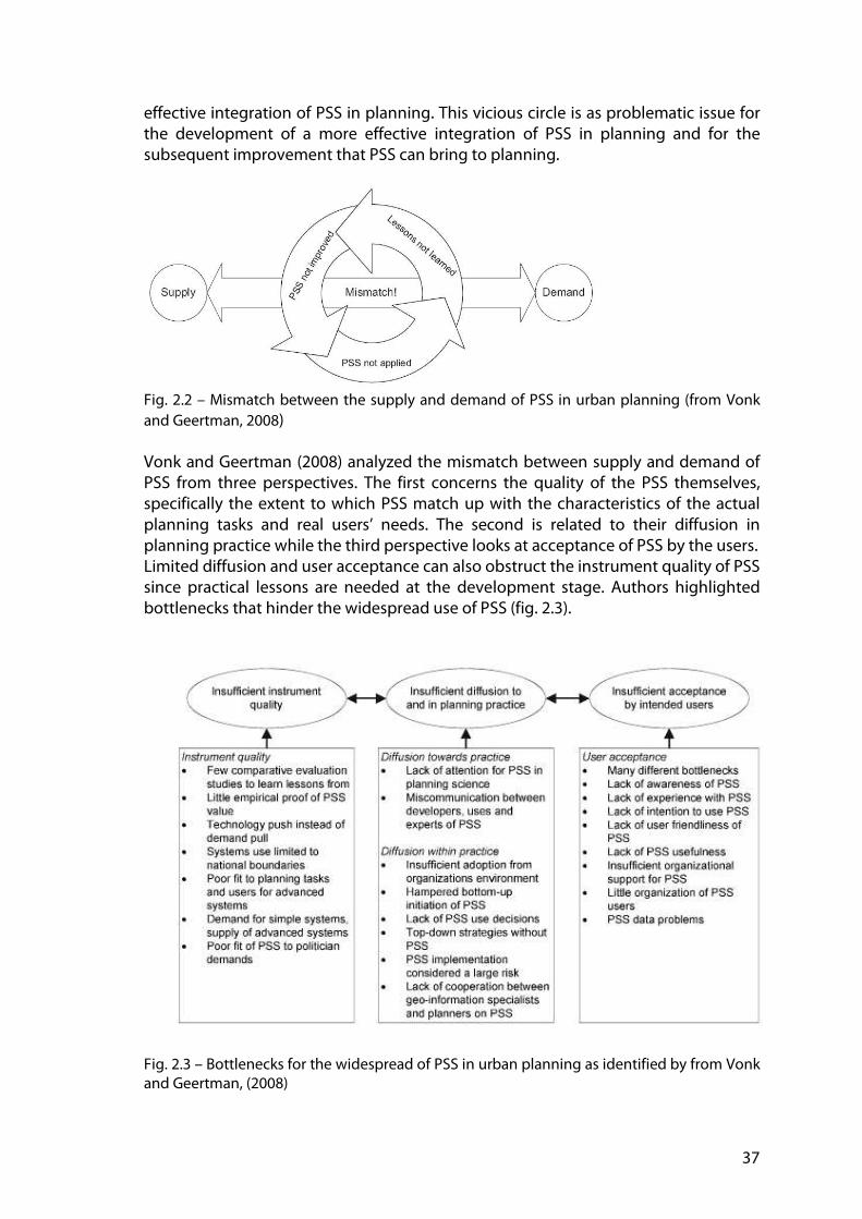
37

effective integration of PSS in planning. This vicious circle is as problematic issue for the development of a more effective integration of PSS in planning and for the subsequent improvement that PSS can bring to planning.

Fig. 2.2 – Mismatch between the supply and demand of PSS in urban planning (from Vonk and Geertman, 2008) Vonk and Geertman (2008) analyzed the mismatch between supply and demand of PSS from three perspectives. The first concerns the quality of the PSS themselves, specifically the extent to which PSS match up with the characteristics of the actual planning tasks and real users’ needs. The second is related to their diffusion in planning practice while the third perspective looks at acceptance of PSS by the users. Limited diffusion and user acceptance can also obstruct the instrument quality of PSS since practical lessons are needed at the development stage. Authors highlighted bottlenecks that hinder the widespread use of PSS (fig. 2.3).

Fig. 2.3 – Bottlenecks for the widespread of PSS in urban planning as identified by from Vonk and Geertman, (2008)

38

To strengthen the effective integration of PSS in the local planning process, tools must combines the embedding of commonly accepted procedures and standards format with clear and simple use, i.e. using easy and familiar GUI. Vonk and Geertman, (2008) identified some “lessons” to be followed in order to remove the bottlenecks for the widespread of PSS in urban planning. The most relevant these lessons are the following: • Research Best Practice of PSS-Supported Planning, identifying methods and procedures found to be most effective. To increase the chances of learning valuable lessons from practice, system developers, that are the ones in charge of PSS development, should be open to learning from planners and to engaging in a continuous dialogue with them. • Develop Advanced PSS Step by Step, applying the so-called mixed model, also known as the spiral model, in the development of the more advanced PSS. The mixed model is an incremental model in which each increment can incorporate either a prototype part or a completely developed part. After the first increments produce ??? a core product, identified core needs, clients of PSS can evaluates the core product and can decide for further increments in the model. • Improving the Quality of Model Based PSS, because many models are not suitable for the characteristics of the planning tasks for which they are designed for. User friendliness is often totally disregarded and models are rarely easy-to-use and can only be operated and understood by a small group of land-use and transport modelling experts. This is partially due to the fact that many models are used for research purposes instead of real applications in planning. • Making PSS Compatible with Regular Office Software. Efforts should be addressed to improve the fit of existing PSS to the skills of those involved in planning • Increased Communication to Practice by Scientists, increasing communication of PSS with planning practice so to improve quality, acceptance and diffusion of PSS. • Instruct Geo-information specialists as Gatekeepers. These professional are those able to follow and evaluate developments in their field of expertise. Therefore they are responsible for capture promising new developments in their field and bringing these to the attention of their managers. Having geo-information specialists for organization that use and develop PSS would primarily improve the diffusion of PSS. • Measure the Benefits of PSS Application, to effectively measure the benefits of applying the diversity of PSS. Such demonstrable benefits are a prerequisite for the widespread acceptance of PSS types. The role of geographic technologies in planning has evolved along with the changing perspectives on planning from scientific approaches through the political process-oriented perspectives and a focus on communication to collective-design approaches. The changing nature of planning has been associated with increased involvement of non-experts (public, interest groups, communities, stakeholders, nongovernmental organization, etc.) into planning and decision making processes. This evolution of planning has occurred together with the increasing accessibility (and user-friendliness) of GIS systems, that have evolved from a close—expert-oriented to an open—user-oriented technology. In short, GIS technology is, yesterday and today, extremely useful in planning but must evolve in parallel with changing perspectives (social, technological, political) of planning.

39

Have all of the new technologies and geo-information applications have brought planners closer to having something we might call a system? Perhaps not, because during the last ten years new tools have appeared but they have remained almost outside of the existing mainstream applications in urban planning. There are no signals so far that this trend would change in the following years. However, it is reasonable to conclude that there are increasing opportunities to make the technologies work together more systematically. The key elements are better networks, better communication protocols, and more integration hooks built into major software products. The System is the realization of this integration. A fundamental help, in this direction, is the diffusion of open source software, that, even in GIS field, is rapidly increasing, especially in public administrations. Anyway, one should always bear in mind that the main aim of PSS is not to replace planner judgments and subsequent decision, but to support her in achieving ‘better’ decisions. The undeniable help, improvement and added value of any spatial model or technology should not be covered by easy-made theoretical justification of unknown social consequences and inequity. PSS may prove valuable tools for enhancing the role of information and knowledge in planning, thereby enabling and facilitating knowledge-based planning. For achieving this, a technocentric approach must be avoided. With many underused PSS available, focus should be put on the demand side, which is the planning community. Researches for the enhancing of PSS must follow the combined interests of communities instead of only pushing forward the a software development which is often un-linked to planner’s real needs.

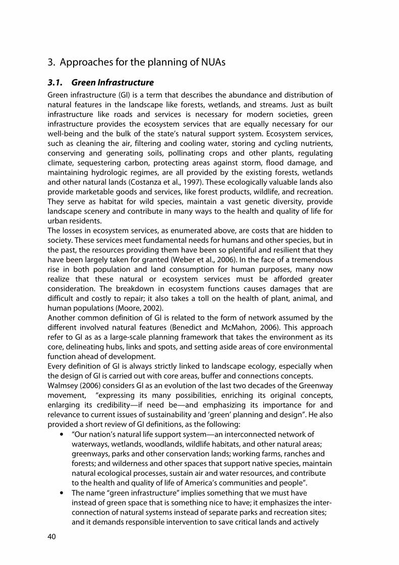
40

3. Approaches for the planning of NUAs

3.1. Green Infrastructure

Green infrastructure (GI) is a term that describes the abundance and distribution of natural features in the landscape like forests, wetlands, and streams. Just as built infrastructure like roads and services is necessary for modern societies, green infrastructure provides the ecosystem services that are equally necessary for our well-being and the bulk of the state’s natural support system. Ecosystem services, such as cleaning the air, filtering and cooling water, storing and cycling nutrients, conserving and generating soils, pollinating crops and other plants, regulating climate, sequestering carbon, protecting areas against storm, flood damage, and maintaining hydrologic regimes, are all provided by the existing forests, wetlands and other natural lands (Costanza et al., 1997). These ecologically valuable lands also provide marketable goods and services, like forest products, wildlife, and recreation. They serve as habitat for wild species, maintain a vast genetic diversity, provide landscape scenery and contribute in many ways to the health and quality of life for urban residents. The losses in ecosystem services, as enumerated above, are costs that are hidden to society. These services meet fundamental needs for humans and other species, but in the past, the resources providing them have been so plentiful and resilient that they have been largely taken for granted (Weber et al., 2006). In the face of a tremendous rise in both population and land consumption for human purposes, many now realize that these natural or ecosystem services must be afforded greater consideration. The breakdown in ecosystem functions causes damages that are difficult and costly to repair; it also takes a toll on the health of plant, animal, and human populations (Moore, 2002). Another common definition of GI is related to the form of network assumed by the different involved natural features (Benedict and McMahon, 2006). This approach refer to GI as as a large-scale planning framework that takes the environment as its core, delineating hubs, links and spots, and setting aside areas of core environmental function ahead of development. Every definition of GI is always strictly linked to landscape ecology, especially when the design of GI is carried out with core areas, buffer and connections concepts. Walmsey (2006) considers GI as an evolution of the last two decades of the Greenway movement, “expressing its many possibilities, enriching its original concepts, enlarging its credibility—if need be—and emphasizing its importance for and relevance to current issues of sustainability and ‘green’ planning and design”. He also provided a short review of GI definitions, as the following:

• “Our nation’s natural life support system—an interconnected network of waterways, wetlands, woodlands, wildlife habitats, and other natural areas; greenways, parks and other conservation lands; working farms, ranches and forests; and wilderness and other spaces that support native species, maintain natural ecological processes, sustain air and water resources, and contribute to the health and quality of life of America’s communities and people”.

• The name “green infrastructure” implies something that we must have instead of green space that is something nice to have; it emphasizes the inter-connection of natural systems instead of separate parks and recreation sites; and it demands responsible intervention to save critical lands and actively

41

practice conservation, regeneration and/or stewardship, instead of something that will take care of itself (Van der Ryn and Cowan, 1996)

Walmsey (2006) also points out some differences between GI and Greenways: • Ecology versus Recreation—Green infrastructure emphasizes ecology, not

recreation • Bigger versus Smaller—Green infrastructure includes large, ecologically

important ‘hubs’ as well as key landscape linkages • Framework for Growth—Green infrastructure can shape urban form and

provide a framework for growth. It works best when the framework pre-identifies both ecologically significant lands and suitable development areas.” (Benedict and McMohan, 2002b, p. 13)

It has to be said that, sometimes, these differences can be very blurred and the two terms are used in the practice as synonymous. The concept of GI is an upgrade of the concept of urban greenspace systems, emerging as a coherent planning entity (Sandstrom, 2002). It can be considered to comprise of all natural, semi-natural and artificial networks of multifunctional ecological systems within, around and between urban areas, at all spatial scales. The concept of GI emphasises their multifunctional role (Sandstrom, 2002), and the importance of connections between habitats . Tzoulas et al. (2007) reviewed the role of GI in the provision of ecosystem services and the importance of GI for human health. The authors also underlined the proactively planning of GI: “Such a planned approach would offer many opportunities for integration between urban development, nature conservation and public health promotion” and therefore would be able to provide different and well valued Ecosystem services in urban areas.. Fig. 3.1 summarize the possible approaches to GI design and management

42

Fig. 3.1. Relationship between scale and design strategies for GI approaches (source: www.greeninfrastructure.net) Benedict and McMahon, 2006) have defined Ten Principles of Green Infrastructure, in order to “provide a strategic approach to and a framework for conservation that can advance sustainable use of land while benefiting people and nature.”

1. Connectivity is key. 2. Context matters. 3. Green infrastructure should be grounded in sound science and land-use planning theory and practice. 4. Green infrastructure can and should function as the framework for conservation and development. 5. Green infrastructure should be planned and protected before development. 6. Green infrastructure is a critical public investment that should be funded up front. 7. Green infrastructure affords benefits to nature and people. 8. Green infrastructure respects the needs and desires of landowners and other stakeholders. 9. Green infrastructure requires making connections to activities within and beyond the community. 10. Green infrastructure requires long-term commitment.

According to these authors the importance of these principles relies on their use “as benchmarks for incorporating a green infrastructure approach into existing planning activities”. Green infrastructure is different from conventional approaches to conservation because it looks at conservation actions together with land development and growth management. Other conservation approaches typically are undertaken in isolation

43

from—or even in opposition to—development. In addition, green infrastructure employs planning, design and implementation approaches similar to those used for roads, water management systems, and other community support facilities.

3.2. Urban ecological networks

Network thinking is not new to ecology. Great ecologists such as Lindenman and Odum have used networks to represent and describe ecological patterns and functions like food webs (Bascompte, 2007). Most recently Margalef, for example, entitled a book chapter ‘‘Ecological Networks’’ (Margalef, 1991). An important application of networks in ecology is the spatial networks approach, related to landscape ecology applications. Graph theory was brought into landscape ecology as a way to generalize the consequences of habitat loss for patch connectivity and its implications for metapopulations (Bascompte, 2007). However, not many works dealt with ecological networks until the last 10 years, when there has been a rapid increase of papers on spatial networks. But it can be said that new works are describing what is well known, which is the metapopulation theory that describe networks of patches. The ecological network concept was already developed in urban planning by the beginning of the 20th century, in the great metropolitan areas in both the Eastern And Western Europe. Green-belt systems were developed to interconnect the city and the nature areas or forest zones and related plans were developed in London as well as Moscow (Jongman et al., 2004). The concept is based on the division of the land territory between the urban area and the natural environment (Antrop, 2004), the construction of an ecological landscape network may be able protect diversity and enhance the exchange of materials and energy (Schrijnen, 2000) through connecting conservation areas, areas of limited development, and greenways, parks, and other ecological ‘‘stepping stones’’ within cities. The ecological network is a consolidated concept but also a strategy for biodiversity protection and environmental optimization, that can be applied at various scales. The basic function of an ecological network is to provide paths for wildlife, energy, and other materials to move and exchange in a fragmented landscape. Its configuration can be summarized at the regional, landscape, and patch scales based on related research. The ecological network approach, promoted by many European countries has been one of the main and fundamental issues of the Action Theme 1 of the Pan European Biodiversity Strategy (Council of European Union 1997) for biological and landscape biodiversity conservation, as included in articles 3 and 10 of the 1992 “Habitat” Directive. Today, in many European regions, the ideas about ecological networks have developed into various concepts and plans for terrestrial systems of ecological stability, or networks of linear habitats connecting habitat islands on different geographical and administrative levels. Jongman et al. (2004) reviewed the result of European efforts to develop ecological greenway networks by developing plans, literature and documents and by consulting different national and regional experts. Different results of the survey highlighted common principles and differences applied in European countries, related to context of geographical, bio-climatic, cultural and political conditions, which again are embedded in different scientific, planning, nature conservation and policy traditions.

44

Although ecological networks have the potential to fulfill multiple functions, so far, they have predominantly been implemented for single functions, such as biodiversity or recreation. Comprehensive network are now receiving mounting attention from planners around the world and many studies are pointing to the importance and feasibility of integrating multiple functions in the network. The priority principle is used to effectively emphasise specific interests when constructing greenways (Teng et al., 2011). Multi-purpose greenway planning, in a similar way to ecosystem conservation planning, should seek to maximise multiple functions while operating under financial and land limitations.

Network Design Principles

Today it is widely accepted (Baldock and others 1993; Council of Europe 2000; ECNC 2006; Jongman 2004) that ecological networks can be structured in four main components:

• a core area, zones of high natural value needing protection (biotopes, system of biotopes, habitat);

• ecological corridors, defined as biological or bio-corridor, linear and continuous structures with different forms and dimensions which interconnect the core areas allowing migration processes, dispersion, and genetic interchanges and improving the cohesion of the ecosystem and biodiversity;

• stepping zones or natural spotting spread areas, particularly important for their strategic position and composition. They are landscape components with small areas useful for hosting migrating species or specific microhabitats in particularly adverse external conditions (i.e. a small marsh in rural areas);

• buffer zones, ecotonal or transitional areas located around the core areas assuring the progressiveness of habitat changes and protecting some elements of the network from potentially negative pressures, i.e. pollution or interferences.

Experiences of ecological network planning and development are often related to continental or national scale (Jongman and others 2004; ECNC 2006), while approaches for defining networks at smaller scales (i.e. at municipality or provincial level) are less diffuse (Magoni and Steiner 2001; Zhang and Wang 2006; Gurrutxaga and others 2010).

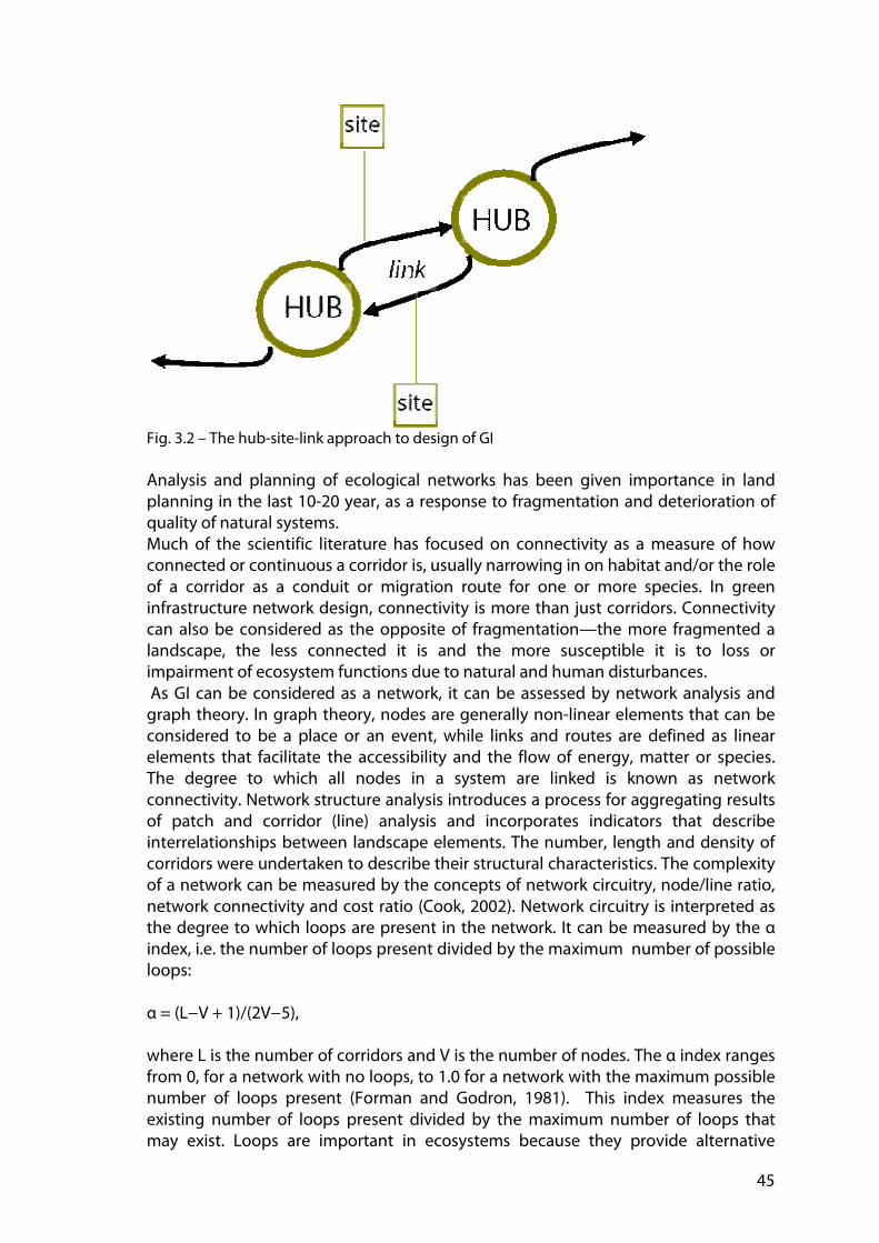
45

Fig. 3.2 – The hub-site-link approach to design of GI

Analysis and planning of ecological networks has been given importance in land planning in the last 10-20 year, as a response to fragmentation and deterioration of quality of natural systems. Much of the scientific literature has focused on connectivity as a measure of how connected or continuous a corridor is, usually narrowing in on habitat and/or the role of a corridor as a conduit or migration route for one or more species. In green infrastructure network design, connectivity is more than just corridors. Connectivity can also be considered as the opposite of fragmentation—the more fragmented a landscape, the less connected it is and the more susceptible it is to loss or impairment of ecosystem functions due to natural and human disturbances. As GI can be considered as a network, it can be assessed by network analysis and graph theory. In graph theory, nodes are generally non-linear elements that can be considered to be a place or an event, while links and routes are defined as linear elements that facilitate the accessibility and the flow of energy, matter or species. The degree to which all nodes in a system are linked is known as network connectivity. Network structure analysis introduces a process for aggregating results of patch and corridor (line) analysis and incorporates indicators that describe interrelationships between landscape elements. The number, length and density of corridors were undertaken to describe their structural characteristics. The complexity of a network can be measured by the concepts of network circuitry, node/line ratio, network connectivity and cost ratio (Cook, 2002). Network circuitry is interpreted as the degree to which loops are present in the network. It can be measured by the α index, i.e. the number of loops present divided by the maximum number of possible loops: α = (L−V + 1)/(2V−5), where L is the number of corridors and V is the number of nodes. The α index ranges from 0, for a network with no loops, to 1.0 for a network with the maximum possible number of loops present (Forman and Godron, 1981). This index measures the existing number of loops present divided by the maximum number of loops that may exist. Loops are important in ecosystems because they provide alternative

46

migration routes for organisms and stable configurations that prevent disturbances (fig. 3.3) Node/links degree can be measured by the β index, which is the number of links divided by the number of nodes: β = L/V. When β is smaller than one, than the network takes on a dendroid pattern. When β is equal to one, than there is single loop in the network. When β is bigger than one, it means that there is more complex connectivity in the network. Network connectivity can be measured by the γ index, the ratio of the number of links in a network to the maximum number of links possible: γ = L/3(V−2). The γ index varies from 0, indicating that none of the nodes is linked, to 1.0, where every node is linked to every other possible node (Forman and Godron, 1981). These measurements are all strongly correlated because they are all based on the same two measurements L and V. This index is useful for assessing the efficacy of the network in terms of the stability of the whole structure. High connectivity degrees mean higher interactions or movements of animals, plants, heat energy, water, and materials among landscape features (fig. 3.4). The indices have been widely used for designing urban ecological network in different areas in the world (Cook, 2002; Zhang and Wang, 2008).

γ = L/3(V-2)

Fig. 3.3 -Example of calculation of the Connectivity index

L=2

V=3

L=3

V=3

L=4

V=4

L=6

V=4

Y=2/3=0,67

Y=3/3=1

Y=4/6=0,67

Y=6/6=1 L=14

V=6 Y=14/12=1,2

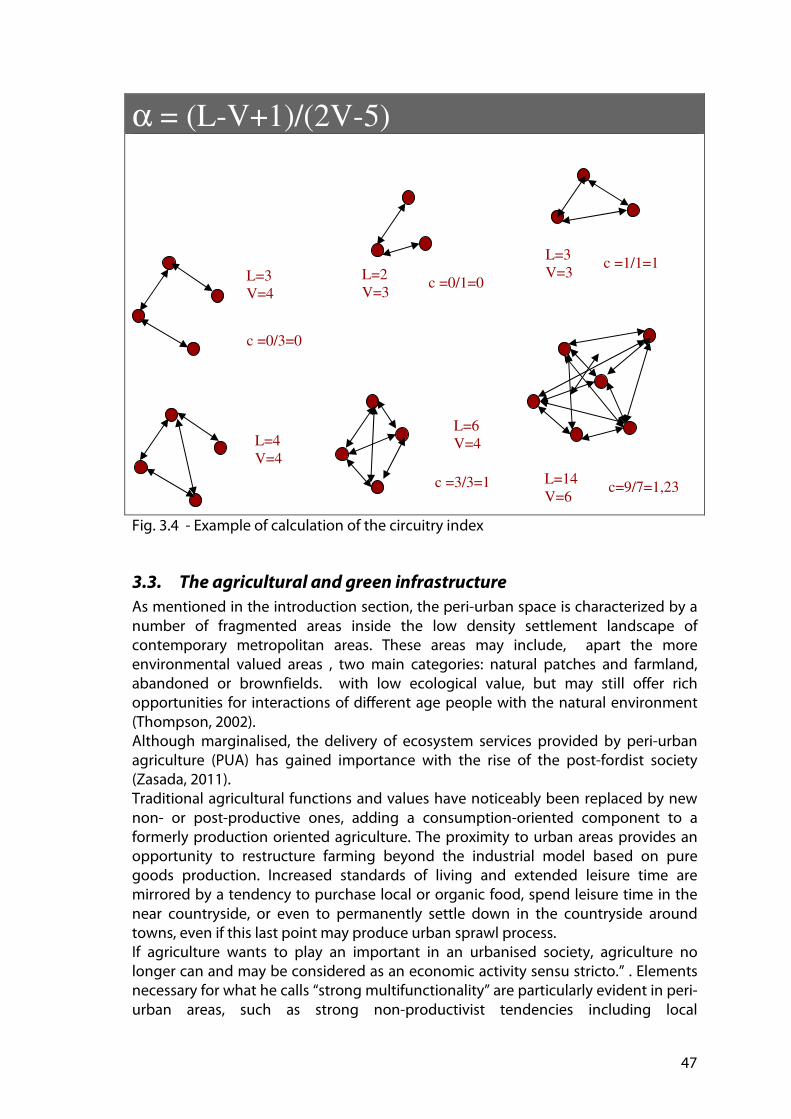
47

α = (L-V+1)/(2V-5)

Fig. 3.4 - Example of calculation of the circuitry index

3.3. The agricultural and green infrastructure

As mentioned in the introduction section, the peri-urban space is characterized by a number of fragmented areas inside the low density settlement landscape of contemporary metropolitan areas. These areas may include, apart the more environmental valued areas , two main categories: natural patches and farmland, abandoned or brownfields. with low ecological value, but may still offer rich opportunities for interactions of different age people with the natural environment (Thompson, 2002). Although marginalised, the delivery of ecosystem services provided by peri-urban agriculture (PUA) has gained importance with the rise of the post-fordist society (Zasada, 2011). Traditional agricultural functions and values have noticeably been replaced by new non- or post-productive ones, adding a consumption-oriented component to a formerly production oriented agriculture. The proximity to urban areas provides an opportunity to restructure farming beyond the industrial model based on pure goods production. Increased standards of living and extended leisure time are mirrored by a tendency to purchase local or organic food, spend leisure time in the near countryside, or even to permanently settle down in the countryside around towns, even if this last point may produce urban sprawl process. If agriculture wants to play an important in an urbanised society, agriculture no longer can and may be considered as an economic activity sensu stricto.” . Elements necessary for what he calls “strong multifunctionality” are particularly evident in peri-urban areas, such as strong non-productivist tendencies including local

L=2

V=3

L=3

V=3 L=3

V=4

L=6

V=4

c =0/1=0

c =1/1=1

c =0/3=0

c =3/3=1 L=14

V=6 c=9/7=1,23

L=4

V=4

48

embeddedness, short supply chains, low farming intensity, a high degree of diversification, and open-minded societies (Wilson, 2007). In his comprehensive review on PUA, Zasada (2011), identifies variety of activities and diversification approaches within the context of environmental, social and economic functions of agriculture that demonstrate how agriculture in peri-urban areas plays a fundamental role in the present and future of metropolitan areas. At the end of the review, the author argued about the ways the preservation of farmland along in the peri-urban area is carried out with. “The main idea of these concepts is to geographically define zones, adjacent to urban areas (where urban development is prohibited or limited) to prevent encroachment of urban sprawl into the periurban open spaces. However, the actual impact of these zoning measures on land preservation is a moot point. Not limiting urbanisation potential in general, restrictions within the open space zones only redistribute development pressure to areas adjacent to them”. Generally, natural areas received high valuation by the public from an environmental perspective, while farmland is only given a marginal interest in peri-urban areas. More societal acknowledgement is required for the functions and values agriculture can provide the urban public, such as local food and comparably cost-efficient provision of landscape features. For this reason, planning has been not capable of addressing the small-scale functional transformations of peri-urban farmland beyond physical land cover changes. According to these issues, the GI should include the agriculture in its approach. If green areas act as an infrastructure for the well-being of contemporary society, it cannot be denied that like roads and services is necessary for modern societies, agricultural areas must be included in this infrastructure of spaces providing ES. The infrastructure is not only Green, but could also be Brown, Yellow or whatever other color farmlands may be. This is also more relevant if the agricultural and green infrastructure is not aimed only at conservation purposes. In our approach very different can be landscape types and land uses that can be part of an infrastructure of land uses that provide different ecosystem services. As it will be discussed in section 5.5 seven different Land-Use Types will be identified, with different strategic purposes: : environmental protection, leisure, local green services and urban agriculture. This difference in purposes make necessary to re-configure the nature of links and connection that can be established, as well as the number and kind of NUAs that can be connected. There is therefore a need for decision-support tools that not only includes mere agricultural production criteria, but also consider covers the provision of the multiple social and ecological functions of agriculture and other Non-Urbanised areas.

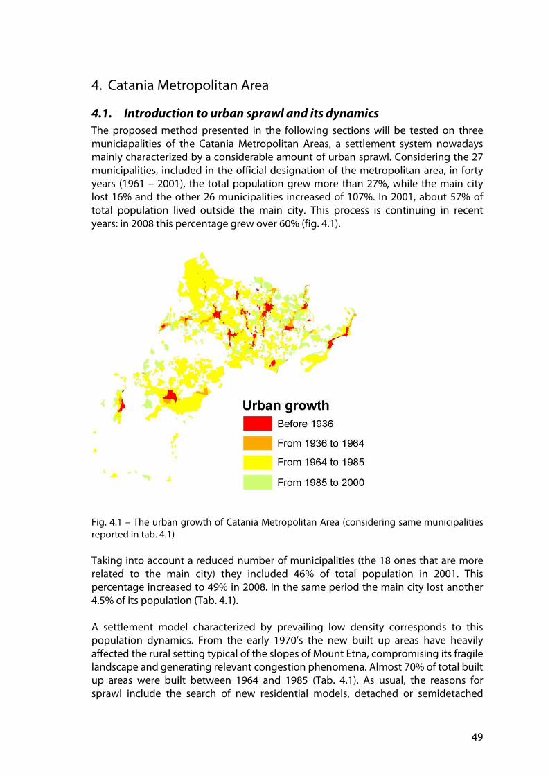
49

4. Catania Metropolitan Area

4.1. Introduction to urban sprawl and its dynamics

The proposed method presented in the following sections will be tested on three municiapalities of the Catania Metropolitan Areas, a settlement system nowadays mainly characterized by a considerable amount of urban sprawl. Considering the 27 municipalities, included in the official designation of the metropolitan area, in forty years (1961 – 2001), the total population grew more than 27%, while the main city lost 16% and the other 26 municipalities increased of 107%. In 2001, about 57% of total population lived outside the main city. This process is continuing in recent years: in 2008 this percentage grew over 60% (fig. 4.1).

Fig. 4.1 – The urban growth of Catania Metropolitan Area (considering same municipalities reported in tab. 4.1) Taking into account a reduced number of municipalities (the 18 ones that are more related to the main city) they included 46% of total population in 2001. This percentage increased to 49% in 2008. In the same period the main city lost another 4.5% of its population (Tab. 4.1). A settlement model characterized by prevailing low density corresponds to this population dynamics. From the early 1970’s the new built up areas have heavily affected the rural setting typical of the slopes of Mount Etna, compromising its fragile landscape and generating relevant congestion phenomena. Almost 70% of total built up areas were built between 1964 and 1985 (Tab. 4.1). As usual, the reasons for sprawl include the search of new residential models, detached or semidetached

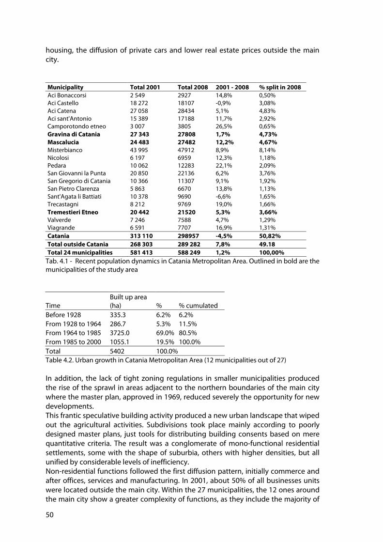
50

housing, the diffusion of private cars and lower real estate prices outside the main city. Municipality Total 2001 Total 2008 2001 - 2008 % split in 2008

Aci Bonaccorsi 2 549 2927 14,8% 0,50% Aci Castello 18 272 18107 -0,9% 3,08% Aci Catena 27 058 28434 5,1% 4,83% Aci sant'Antonio 15 389 17188 11,7% 2,92% Camporotondo etneo 3 007 3805 26,5% 0,65% Gravina di Catania 27 343 27808 1,7% 4,73%

Mascalucia 24 483 27482 12,2% 4,67%

Misterbianco 43 995 47912 8,9% 8,14% Nicolosi 6 197 6959 12,3% 1,18% Pedara 10 062 12283 22,1% 2,09% San Giovanni la Punta 20 850 22136 6,2% 3,76% San Gregorio di Catania 10 366 11307 9,1% 1,92% San Pietro Clarenza 5 863 6670 13,8% 1,13% Sant'Agata li Battiati 10 378 9690 -6,6% 1,65% Trecastagni 8 212 9769 19,0% 1,66% Tremestieri Etneo 20 442 21520 5,3% 3,66%

Valverde 7 246 7588 4,7% 1,29% Viagrande 6 591 7707 16,9% 1,31% Catania 313 110 298957 -4,5% 50,82%

Total outside Catania 268 303 289 282 7,8% 49.18

Total 24 municipalities 581 413 588 249 1,2% 100,00%

Tab. 4.1 - Recent population dynamics in Catania Metropolitan Area. Outlined in bold are the municipalities of the study area

Time Built up area (ha) % % cumulated

Before 1928 335.3 6.2% 6.2% From 1928 to 1964 286.7 5.3% 11.5% From 1964 to 1985 3725.0 69.0% 80.5% From 1985 to 2000 1055.1 19.5% 100.0% Total 5402 100.0% Table 4.2. Urban growth in Catania Metropolitan Area (12 municipalities out of 27) In addition, the lack of tight zoning regulations in smaller municipalities produced the rise of the sprawl in areas adjacent to the northern boundaries of the main city where the master plan, approved in 1969, reduced severely the opportunity for new developments. This frantic speculative building activity produced a new urban landscape that wiped out the agricultural activities. Subdivisions took place mainly according to poorly designed master plans, just tools for distributing building consents based on mere quantitative criteria. The result was a conglomerate of mono-functional residential settlements, some with the shape of suburbia, others with higher densities, but all unified by considerable levels of inefficiency. Non-residential functions followed the first diffusion pattern, initially commerce and after offices, services and manufacturing. In 2001, about 50% of all businesses units were located outside the main city. Within the 27 municipalities, the 12 ones around the main city show a greater complexity of functions, as they include the majority of

51

value added services and productions (Martinico, 2005). Among these last ones there is a group of 5 municipalities (Aci Castello, Gravina, S. Agata Li Battiati, San Gregorio and Tremestieri Etneo) where, not only the built up areas, but also the social and economic profiles are almost undistinguishable from the main city. Data about household size, age, workforce and literacy are almost similar to the ones surveyed in Catania. Land use planning is characterized by a complete lack of overall metropolitan planning. Each municipality has its own master plan based on autonomous choices as far as the amount of new developments is concerned. The only attempt to define a plan at metropolitan level failed in 1960s, (Martinico, 2005). This piecemeal approach has caused a notable erosion of the residual agricultural land, progressively substituted by new developments. Agricultural land and other Non-Urbanised areas in Catania metropolitan area have never been studied systematically in spite of their strategic role. This lack of rigorous data collection and analyses is the direct consequence of the weakness of regional planning. On the contrary, the study of these areas is strategic both for defining agricultural, urban and infrastructural policies and for proposing climate change adaptation strategies, including in the process elements like their permeable and evapotranspiring features. It appears clear that only by pursuing a planning strategy at metropolitan level, going beyond the traditional municipal plans, it is possible to envisage a way to restore the grid of Non-Urbanised areas that has been broken by over thirty years of unwise urban development, assuming an effective stance about climate change issues.

4.2. Municipalities of Mascalucia, Gravina di Catania and Tremestieri

Etneo

Mascalucia, Gravina di Catania and Tremestieri Etneo (fig. 4.2) show the same feature of extensive urban sprawl as the one identified in the entire Catania metropolitan area (fig. xx). The settlement model corresponds to this population dynamics. From the early 1970’s the new built up areas have heavily affected the rural setting on the slopes of Mount Etna, eroding its fragile agricultural landscape and generating relevant congestion phenomena. The reasons for sprawl include the search of detached or semidetached houses, the diffusion of private cars and lower real estate prices outside the main city. The three municipalities considered are small agricultural towns on the Mt. Etna slopes that have been absorbed into the expanding metropolis. According to national census data, the increase in the total population has been constant since 1936, when they summed up about 6000 inhabitants, with a sudden boost from 1971 on. In 2008 population reached more than 77000 inhabitants. Agriculture oriented economy, mainly based on wine production, was completely swiped out by holiday houses in the 1960-1970s and in the following 20 years many of these houses have become stable dwellings. Built up areas increased by more than 2000 % between 1928 and 2008 (Fig. 4.3 and tab. 4.3)

52

Fig. 4.2 -. The study area of the three municipalities of Mascalucia, Gravina di Catania and Tremestieri in the Catania Metropolitan Area (Italy).

Fig. 4.3 – Example of urban growth dynamic for Mascalucia

53

Table 4.3 -Urban growth in Mascalucia municipality

Time

Built up area (ha) % % cumulated

1928 35.7 4.74% 4.74% 1928-1964 47.7 6.32% 11.06% 1964-1985 454.3 60.24% 71.30% 1985-2000 173.3 23.04% 94.34% 2000-2008 42.1 5.66% 100%

TOT 753 100.00%

4.3. Land Use

The initial step of this study was the construction of the first detailed land use map ever produced for this area. It is based on: vector cartography (1:10 000) produced by regional authorities, municipal vector cartography (1:2000), field surveys and 2008 orthophotos. Land uses are mapped in fig. 4.4 and summarized in table 4.4. Built up areas cover almost half of the municipality. The rest is distributed among farmlands and abandoned farmlands, woods and shrubs and parks and public gardens. Roads total almost 10 % of the total. In order to better differentiate the urban fabric for the Land Cover Analysis, Residential patches have been further divided in the following categories: historical compact urban settlements, multi-storey apartment residences, linear historical rural settlements and detached houses. Linear historical settlements are a typical pattern of this area and they are formed by rows of narrow plots of farmland with houses aligned along the old roads that connect historical towns. In the rest of the study, NUAs include the following land-use types

• abandoned farmlands • farmlands • woods • shrubs • parks and public gardens.

Farmlands and woods and shrubs play an important role in controlling evapotranspiring processes and in mitigating urban pollution inside highly urbanized settlements. Woods have been traditionally replaced by agriculture. The development pressure in the examined metropolitan area is now threatening this agricultural land. A relevant feature is the amount of small patches of abandoned farmlands. A large suburban park is the main component of parks and public gardens land use type. In addition, this includes other small areas with a traditional layout characterized by prevailing paved areas and inadequately designed playgrounds. Patches of land use belongin to these categories will be used as the base for all

the analysis useful for the characterization of Non-Urbanised Areas.

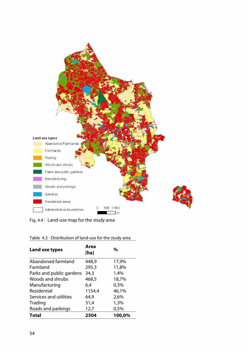
54

Fig. 4.4 - Land-use map for the study area Table 4.3 -Distribution of land-use for the study area

Land use types Area

[ha] %

Abandoned farmland 448,9 17,9% Farmland 295,3 11,8% Parks and public gardens 34,3 1,4% Woods and shrubs 468,5 18,7% Manufacturing 6,4 0,3% Residential 1154,4 46,1% Services and utilities 64,9 2,6% Trading 31,4 1,3% Roads and parkings 12,7 0,5%

Total 2504 100,0%

55

5. Characterization of NUAs for urban planning: methodology and results

5.4. The analytical phases of Suitability Analysis for NUAs

A methodology is proposed to characterize the patches of NUAs, in order to identify new land uses to conserve and enhance the provided ecosystem services. The methodoky is composed of five different phases, all performed with GIS. A Land Cover Analysis (LCA) is used to evaluate evapotranspiration of the different land-use types based on their land cover composition. With a Fragmentation Analysis (FA), every patch of NUA is assigned a value of fragmentation, taking into account its dimension and density. A Proximity Analysis (PA) is conducted to evaluate the proximity of residential parcels to NUAs and to quantify the number of people that have access to NUAs. Combining these sets of results, a first option for new land uses of NUAs is proposed in a Land-Use Suitability Matrix. The last analytical step verifies the correspondence of proposed new land uses with the current ones, using a Compatibility Matrix.

5.5. Land cover analysis

5.5.1. From land-use to land cover

The traditional land use categories are generally not sufficient to provide indication about land cover features. A patch of a specific land use type can be composed by a complex mix of land covers. In order to evaluate the evapotranspiration degree of each land use types, it becomes crucial their characterization by identifying different land covers. The concepts of land use and land cover are often mixed up an this confusion have created problems for research and other activities that seek to integrate different land data as land cover and land use are fundamentally distinct. Mixing of the concepts of land cover and land use has become so prevalent that classifications of ‘pure’ land use or land cover are rare even when that is the stated objective (Di Gregorio and Jansen, 2000). The historical reasons for the confusion of these concepts mostly relate to the different mapping needs of the different agencies involved and the ability to statistically process digital remotely sensed data (Comber, 2008). Particularly, land cover is all that can be observed on the surface of the earth (Di Gregorio and Jansen, 2000) while land-use is referred to the way in which these biophysical assets are used by humans (Cihlar and Jansen, 2001). In some respects, there is a close relationship between land cover and land-use because use depends on land features (i.e. cover, morphology, position, substratum, etc.). Land cover can be determined by direct observation of the earth’s surface while land use is a socio-economic interpretation of the activities that take place on that surface (Fisher et al, 2005). On the other side, land use cannot be derived automatically from land cover observation for many interrelated causes. For instance, individuals can use differently an area, being equal the land cover type, depending on the benefits they expect, considering their aims, their available means, the possible constraints and the given set of biophysical parameters. In addition, there are other determining factors such as institutional and cultural constraints, legal attributes of the plot (derived from land tenure or planning) and socio-economic conditions (Cihlar and Jansen, 2001).

56

Consequently, land use and land cover analysis need different approaches and survey tools. There is a need for their separation to support modelling activities (GLP, 2005), to better link observed changes in the earth’s surface with socio-economic process (Brown et al, 2000) and to promote a culture of consistency in land survey reporting (Comber 2008). The separation of land cover and land use may also facilitate the integration of land data for environmental modelling and planning activities. Land use and land cover have to be maintained as distinct concepts, since their data primitives are different (Comber 2008). Moreover, land cover analysis is widely based on aerial photographs and satellite images interpretation. The analysis of aerial photographs for producing land cover maps is based on classification systems. The precision of mapping can vary, depending on how each land cover type is identified on the ground. The classification system is guided by a set of rules to be used by the human interpreter or built in the software. However, the final decision on how to classify a single plot, in terms of cover types, depends on the analyst’s knowledge, skills and on subjective interpretation. The human mind has the capability to use a lot of additional information useful for better understanding aerial photographs. This is commonly known as field experience or understanding of the landscape and it represents an extrinsic factor contributing to the reliability of land cover maps based on interpretation of aerial photographs (Strand et al, 2002).

5.5.2. Geographical Sampling for Evapotranspiration assessment

In our approach, a geographic sampling is here proposed for land cover assessment of land use types, interpreting the contribution of various authors (Gill 2003; Akbari et al 2003; Tappan et al 2004). Different approaches for determining urban surface cover are discussed in the literature. At the conurbation scale surface cover analyses are generally undertaken using remotely sensed imagery. A range of satellite and aerial imagery have been used, including many photographic sources, (Akbari et al., 2003; Myeong et al., 2001). Satellite imagery has increasing resolution and capabilities. However, automatic classifications using remotely sensed data are still a complex procedure in urban areas with misclassifications and confusion between surface covers (Myeong et al., 2001). Non-automatic approaches using high spatial resolution aerial photography may still be more appropriate for accurately characterising the urban environment (Akbari et al., 2003; Myeong et al., 2001). Aerial photograph interpretation is an establishedmethod for determining surface cover (Akbari et al., 2003) that has been shown to be both accurate and cost-effective (Butz and Fuchs, 2003). A common approach at the conurbation level is to disaggregate the urban area into distinctive strata, based on land use or morphology, and use this as a basis for a sampling strategy (Nowak et al., 2003; Pauleit and Duhme, 2000). This allows for samples to be taken from more homogeneous categories and thus leads to more precise results (Nowak et al., 2003). In the evaluation of evapotranspiring surfaces, surveys and mapping have to be conducted at a very detailed scale, in order to identify those land cover surfaces (i.e trees, small grass or urban gardens) within the different land use types. Evapotranspiration assessment at lower scales would not have been feasible as it would require a manual digitalization of every land cover feature. In order to speed up process in such typical time consuming task, geographical random sampling of land use patches has been used to reduce the number of land cover features to be

57

identified and mapped. Random sampling is usually carried out when the area under study is very large, or time available is limited. In this research, eight land cover types were chosen (fig. 5.1): buildings, impervious surfaces (roads driveways, sidewalks, parking areas), grass, cultivated, trees, shrubs, herbaceous vegetation and bare soil. The proposed sampling method is based on the overlaying of 30 meters square vector grid over the land use map (fig. 5.2, left) and on a random choice of cells of the grid (fig. 5.2, right). Within each of them, land cover types have been identified by orthophoto interpretation. A key step was the choice of the appropriate sample size (Bartlett et al. 2001). Within a quantitative survey design, determining sample size and dealing with nonresponse bias is essential. “One of the real advantages of quantitative methods is their ability to use smaller groups of people to make inferences about larger groups that would be prohibitively expensive to study” The question then is, how large of a sample is required to infer research findings back to a population?

Buildings

Cultivated

Impervious

Shrubs

Trees

Herbaceous vegetation

Bare soils

Grass

Fig.5.1 - Land cover types identified in the study area For each land use type, the sample size was calculated using Cochran formulas for categorical data (Bartlett et al. 2001). Formulas calculate the number of appropriate sample size in survey research, given a certain population (the number of overlayed grid cells) and a pre-defined confidence interval. Sample size is expressed for categorical data by:

( )2

2

0

1

c

ppZss

−××=

where: sso is the sample size; Z equals to 1,96 for a confidence level of 95%. p is the standar deviation, fixed p at 0.5; c is confidence interval, fixed in 0.05;

( )pp −× 1 is the estimate of the variance;

When sample size exceeds 5% of the population, formula is corrected in the following way.

58

pop

ss

ssss

0

01

1+

= ,

where: ss1 is the corrected sample size; pop is the population, which, in our case, is represented by the total number of cells for each land use category. Confidence level and interval was fixed respectively at 95 % and 5%. Sample cells were randomly generated with the Random Selection ArcMap tool. Percentage of sampled cells for each land use types are summarized in tab. 5.1. Since land use types differ in geographic distribution and size, it was important to sample each of them with samples of different size.

Fig. 5.2 - The overlayed sampling grid on semi-detached house land use (left) and a detail of the random generated sampling cells (right) for the municipality of Mascalucia

59

Tab. 5.1 - Sampled cells for the different land use types Mascalucia Tremestieri Etneo Gravina di Catania

Land use

types

# of

cells # sampled

cells % # of cells # sampled

cells %

# of

cells # sampled

cells %

Detached

houses 7280 364 5 1744 314 18 260 156 60

Historical

compact

settlements 366,7 187 51 249 152 61 60 52 87

Multi-storey

apartment

residences 714 250 35 717 251 35 2006 321 16

Linear

historical rural

settlements 85 70 82 191 128 67 164 115 70

Private

gardens 163 115 70 65 56 86 0 0

Retail 93 75 81 135 100 74 178 121 68

Manufacturing 20 19 95 9 9 98 13 13 100

Services &

utilities 417 200 48 179 122 68 142 104 73

Farmland 1540 308 20 855 265 31 993 278 28

Abandoned

farmland 2187 328 15 2173 326 15 662 245 37

Parks &

public gardens 279 162 58 63 54 86 62 54 87

Woods &

shrubs 3470 347 10 900 270 30 816 261 32

Roads &

parkings 18900 378 2 9225 369 4 7280 364 5

Fig. 5.3 plots the percentages of sampled cells against the total number of cells for each land use type (including, as an example, only the municipality of Mascalucia). The percentage of sampled cells decreases exponentially as the number of cells increases, meaning that more extended land use types need a lower percentage of cells to be sampled.

60

0%

10%

20%

30%

40%

50%

60%

70%

80%

90%

0 1000 2000 3000 4000 5000 6000 7000 8000

Fig. 5.3 - Percentage of sampled cells against total number of cells for the land use types of Mascalucia Inside every sampled cell, land cover types were manually identified and digitalized by photo interpretation of orthophotos (taken in October 2007), as shown in fig. 5.4. Thanks to the high resolution of orthophotos (0.25 meters), a very detailed feature extraction was possible (minimum mapped area of 30 m2).

Fig. 5.4 - Example of the land cover surfaces extraction (B = Buildings, G= Grass, T = Trees, I = Impervious, BS= Bare soils)

5.5.3. Results

Results of Land Cover Analysis are shown in Table 5.2, where for each land use type the composition of land cover surfaces is reported. The highest buildings land cover type is found in Linear historical rural settlements (45%), in Historical compact settlements (44%) and in Multi-storey apartment residences (30%). Detached houses have only 16%, less than retail and manufacturing (17%) and services & utilities (19%). All other cover types are below 4%.

61

Impervious are high in manufacturing (40%), service & utilities (35%) and retail (31%). Residential land use types present a heterogeneous distribution of this land cover, ranking from 9% in private gardens, linear, followed by Linear historical rural settlements and detached houses (20%), historical compact urban areas (26%), multi-storey apartment residences and services (33%). Tab. 5.2 - Results from land cover surface analysis, showing the different percentages of land covers for each land use

Land cover types percentages [%] Land Use

Type Trees Shrubs Cultivated Grass Herbaceous vegetation

Bare soil

Buildings Impervious TOT

Detached houses

23.71 6.30 5.73 20.81 3.18 3.66 16.49 20.12 100

Historical compact settlements

15.03 1.58 0.64 10.16 2.17 0.53 43.70 26.17 100

Multi-storey apartment residences

19.11 0.88 0.55 4.38 9.01 3.49 29.73 32.84 100

Linear historical rural settlements

18.50 3.71 1.67 5.14 5.20 0.69 45.48 19.61 100

Private gardens

31.14 13.06 6.05 17.88 8.07 2.95 11.52 9.34 100

Retail 7.40 1.83 0.69 3.76 11.07 26.62 17.47 31.17 100

Manufacturing 4.94 1.62 4.79 3.10 11.67 16.25 17.40 40.24 100

Services & utilities

9.31 5.01 2.04 9.17 7.48 12.40 19.33 35.24 100

Farmland 6.94 13.35 51.65 1.13 13.29 7.32 1.64 4.68 100

Abandoned farmland

11.30 28.37 12.11 0.43 28.07 15.21 1.12 3.40 100

Parks & public gardens

67.34 0.95 0.27 9.10 6.14 0.25 2.19 13.77 100

Woods & shrubs

11.52 31.20 4.61 2.09 21.46 19.22 2.10 8.10 100

Roads & parkings

10.43 0.82 0.93 0.53 7.83 5.99 3.61 69.87 100

Trees cover type is higher in parks & public gardens (67%): this result is considerably affected by a large suburban park placed in Mascalucia municipality, characterized by natural woodland. Residential land use types show the highest proportion of trees cover: 15% in historical compact settlements, 24% in detached houses and 31% in private gardens. Farmland (7%), abandoned farmland (11%), woods & shrubs (12%) show less percentages of trees cover. As predictable, the highest grass cover type is found in detached houses (21%), followed by private gardens (18%), historical compact settlements (10%), service & utilities and parks & plublic gardens (9%), slightly more than the one of multi-storey apartments residences (13%). Services & utilities (9%), retail (4%) and manufacturing (3%) show an higher percentage than woods & shrubs (2%). Finally, grass is very low in farmland (1%), due to the features of local agriculture, where grass is almost never present. The high value found for detached houses is related to the fact that lawns are socially appreciated by suburbanites, in spite of high maintenance costs in Sicilian climate.

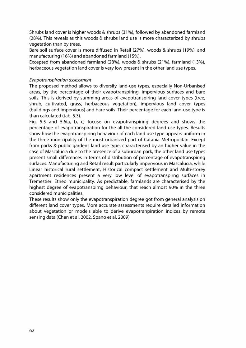
62

Shrubs land cover is higher woods & shrubs (31%), followed by abandoned farmland (28%). This reveals as this woods & shrubs land use is more characterized by shrubs vegetation than by trees. Bare soil surface cover is more diffused in Retail (27%), woods & shrubs (19%), and manufacturing (16%) and abandoned farmland (15%). Excepted from abandoned farmland (28%), woods & shrubs (21%), farmland (13%), herbaceous vegetation land cover is very low present in the other land use types. Evapotranspiration assessment

The proposed method allows to diversify land-use types, especially Non-Urbanised areas, by the percentage of their evapotranspiring, impervious surfaces and bare soils. This is derived by summing areas of evapotranspiring land cover types (tree, shrub, cultivated, grass, herbaceous vegetation), impervious land cover types (buildings and impervious) and bare soils. Their percentage for each land-use type is than calculated (tab. 5.3). Fig. 5.5 and 5.6(a, b, c) focuse on evapotranspiring degrees and shows the percentage of evapotranspiration for the all the considered land use types. Results show how the evapotranspiring behaviour of each land use type appears uniform in the three municipality of the most urbanized part of Catania Metropolitan. Except from parks & public gardens land use type, characterised by an higher value in the case of Mascalucia due to the presence of a suburban park, the other land use types present small differences in terms of distribution of percentage of evapotranspiring surfaces. Manufacturing and Retail result particularly impervious in Mascalucia, while Linear historical rural settlement, Historical compact settlement and Multi-storey apartment residences present a very low level of evapotranspirng surfaces in Tremestieri Etneo municipality. As predictable, farmlands are characterised by the highest degree of evapotranspirng behaviour, that reach almost 90% in the three considered municipalities. These results show only the evapotranspiration degree got from general analysis on different land cover types. More accurate assessments require detailed information about vegetation or models able to derive evapotranpiration indices by remote sensing data (Chen et al. 2002, Spano et al. 2009)

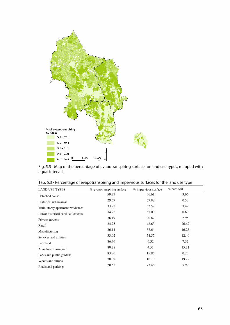
63

Fig. 5.5 - Map of the percentage of evapotranspiring surface for land use types, mapped with equal interval. Tab. 5.3 - Percentage of evapotranspiring and impervious surfaces for the land use type

LAND USE TYPES % evapotranspiring surface % impervious surface % bare soil

Detached houses 59.73 36.61 3.66

Historical urban areas 29.57 69.88 0.53

Multi-storey apartment residences 33.93 62.57 3.49

Linear historical rural settlements 34.22 65.09 0.69

Private gardens 76.19 20.87 2.95

Retail 24.75 48.63 26.62

Manufacturing 26.11 57.64 16.25

Services and utilities 33.02 54.57 12.40

Farmland 86.36 6.32 7.32

Abandoned farmland 80.28 4.51 15.21

Parks and public gardens 83.80 15.95 0.25

Woods and shrubs 70.89 10.19 19.22

Roads and parkings 20.53 73.48 5.99

64

Fig. 5.6a - Percentage of evapotranspiring, impervious surface and bare soils for land use types in Mascalucia municipality

Fig. 5.6b - Percentage of evapotranspiring, impervious surface and bare soils for land use types in Tremestieri Etneo municipality

65

Fig. 5.6c - Percentage evapotranspiring, impervious surface and bare soils for land use types in Gravina di Catania municipality

5.6. Fragmentation Analysis

Fragmentation is the division of contiguous ecosystems into patches. A patch is an area with relatively homogeneous conditions compared with other patches (Forman, 1995). A class typically represents a patch category, e.g. land cover/land use, habitat or vegetation classes. Division of natural ecosystems into smaller patches is the result of human activities (agriculture, development and infrastructure) in places once covered by forests or other natural land uses. Consequences of fragmentation include: increase in the number of patches and in the total length of their edges, decrease in the mean patch size, (Collinge, 2009; Rutledge, 2003). Urban sprawl also tends to affect heavily native habitats by creating isolated remnants (August et al., 1998). There are multiple ways fragmentation is being dealt with in literature, both conceptually and methodologically. The stream of research encompasses two dominant categories can be (Gulinck and Wagendorp, 2002). One category is linked to nature conservation and concentrates on the role of fragmentation for natural biological populations or on the design principles for good defragmenting planning for sustainable ecological landscapes. The second category is more abstract and concentrates on landscape metrics for measuring fragmentation and their complex behaviour in terms of scale, resolution, measurement techniques, inter-correlations and others. These two categories reflect the duality in process and pattern. In the following, some metrics belonging to the second category will be used for fragmentation assessement.

5.3.1. Indicators of fragmentation

Landscape indices used for fragmentation may be divided into non-spatial and spatial (Gustafson 1998). Non-spatial indices describe landscape composition and include measurements of the number of patch classes or proportions of total area. Spatial indices describe patch attributes and contain information relevant to

66

measuring fragmentation. The spatial indices can be further divided into those that describe patch composition, shape and configuration (Rutdlege, 2003). In the strictest sense, only patch composition relates to fragmentation, but the traditional view of ecosystem fragmentation encompasses all three (as well as loss of area). Composition indices describe the basic features of fragmentation. Shape indices quantify patch complexity, which can be important for different ecological processes (Forman 1995). For example, circles or squares have less edge and, potentially, more core area. Other shapes. such as long, narrow features like tree lines, or sinuous features like riparian areas may have comparatively little core area despite a large total area. Patch configuration indices measure the degree of connectedness or, conversely, isolation between and among patches on a landscape. In the proposed Fragmentation Analysis, fragmentation was evaluated for all the patches belonging to land use types considered in NUAs definition (section 5.6). These land use types total about 44% of total municipal area. The choice of a higher number of land use types would have increased fragmentation, since a high number of classes usually increases the number of patches (Turner, 1989) As already introduced, many landscape metrics are used in landscape fragmentation assessment (Forman, 1995; Rutledge, 2003; Ritters et al., 1995). A boost in landscape fragmentation metrics occurred with the development of Fragstats software (McGarigal and Marks, 1995), which provided a powerful tool for calculating landscape metrics at different scales. Studies on landscape fragmentation usually provide a single value for the entire study area. Sometimes, this may not be sufficient to describe fragmentation accurately. An other approach, that is calculating metrics on grid cells as geographical unit, may affect metrics values since cells boundaries usually truncate patches (Gustafson, 1998). A geographical calculation unit, useful for describing patterns at the scale of the study herewith presented, was needed. When indices are used to describe landscape pattern at regional scale, the appropriate spatial unit has to be decided before starting with indices calculation. In other words, a single set of indices calculated over the entire region are not accurate enough to describe the spatial heterogeneity within the region (Liu et al., 1999). The choice of the correct areal unit, also known as Modifiable Areal Unit Problem (Openshaw and Taylor, 1981), is a crucial factor in landscape metrics. The optimal spatial unit was determined by calculating the point at which the indices become stable as the calculation unit increases.

Fig. 5.7 . Examples of different grain cells as calculation units (from Liu et al. 1999) In this study, the geographical unit for fragmentation metrics is the single NUAs patch. This allows a better assessment of the geographical variation of fragmentation, as well as the characterization of each patch with a single score of fragmentation metrics.

67

Chosen metrics are the ones easier to calculate and directly linkable to each patch of NUAs. Two patch composition metrics (Rutledge, 2003) were calculated at patch level: - Patch Area (PA) (McGarigal and Marks, 1995; Turner et al., 1989); - Number of patches within 500 m radius from each patch (NP) (Turner, 1989). PA provides a measure of the area for each patch. Larger patches are usually considered less fragmented (Forman, 1995). NP provides a measure of neighbour density, (fig. 5.8). Being equal the total patch area within the buffer, higher values of NP indicate a more fragmented landscape.

Fig. 5.8 - Example of the 500 m buffer for neighbour patches density in NP metric. The two metrics were aggregated to get a unique fragmentation score: ( ) ( )__1 NPPAFR +−=

Where: FR is the Fragmentation degree for each patch; PA_ and NP_ are the normalized values of PA and NP, in a 0 to 1 scale.

max

_PA

PAPA =

max

_NP

NPNP =

PAmax and NPmax are the maximum values in the study area. PA_ has been turned in (1-PA_) since the metric is in inverse relation to fragmentation.

68

All scores from metrics must be considered as relative among the different patches within the study area.

5.3.2. Results

Table 5.4 reports the results of the FA, including the scores of the PAT, NP and FR indices. The total number of NUA patches being analyzed was 1262, with an average area of 9880 ha. Table 5.4. Scores for the PAT, ND and FR indeces

The PAT scores were characterized by a very high standard deviation (23.46 ha), because many different kind of patches were included in the NUAs of the study area. This is typical of metropolitan areas that include varied patches, ranging from very small abandoned farmlands (less than 0.1 ha) to larger green spaces and farmland (greater than 30 ha). The NP showed a geographically differentiated distribution of scores. Patches that had a high number of neighbor patches were placed in the middle of urban settlements characterized by detached houses. This is an urban configuration that tends to heavily fragment the landscape. The NP values showed a very high fragmentation pattern. This was due to the massive presence of detached houses, especially in the central and western part of the municipality. The NP values ranked from 4 to 84, with an average of 36 and a standard variation of 15.6. Fig. 5.9 maps the results of the FR and scores were classified in 3 equal interval classes, from Lev. 1 (low fragmented patches) to Lev. 3 (high fragmented patches) (fig. 5.10). As a composite index, the FR showed less variation in scores, with a standard variation of 0.12. High degree of fragmentation (Lev. 3) encompassed 819 patches, 64.9% of the total and 67.4% of the area of NUAs. Three clusters of patches were identified: the first in the southern part of the study area, the second one in the eastern part and the third, more dispersed, in the central and northern part. Some correlation with residential land uses was found. This class of fragmentation was the most common in the study area. Patches with medium fragmentation (Lev. 2) were generally widespread among the three municipalities. They were larger patches with medium-high NP values and smaller patches with low NP values. There were 439 patches (34.8% of the total) within this class, comprising 25.3% of the total area. Less fragmented patches (Lev. 1) were much less frequent, with only 4 patches (0.3%) and 7.3% of the total area. They included the larger patches and the ones which featured the lowest NP scores.

Min Max Average Dev. Std

PA 3 37822 9880.68 23458.70

ND 4 135 41.29 15.75

FR 0.628 1.654 1.28 0.12

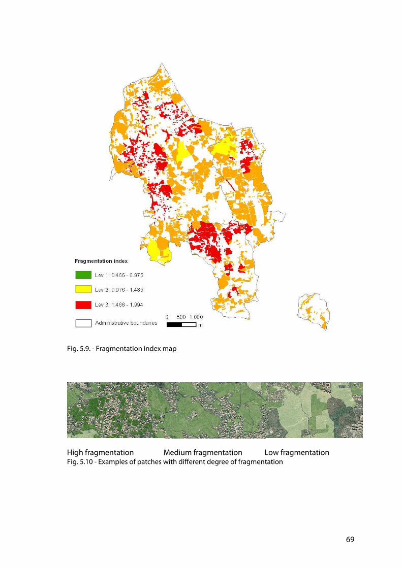
69

Fig. 5.9. - Fragmentation index map

High fragmentation Medium fragmentation Low fragmentation Fig. 5.10 - Examples of patches with different degree of fragmentation

70

5.7. Proximity to residential uses

5.4.1. Definition of Proximity

According to the proposed fragmentation index (section 5.3), NUAs with a high degree of fragmentation are small patches and/or patches that are included in a fragmented neighborhood. Specific land uses may be preferred for these patches, especially those characterized by a high proximity to residential areas. For instance, allotment gardens or playgrounds are typical urban land uses that feature small patches with a good proximity to residential areas. Activities in these areas usually require short times and distances to be reached. For example, children or older people need to walk small distances to get to playgrounds or allotment gardens. One explanation underlying the “attractiveness” of a land use is the utility associated with the activity to be conducted at the destination. This is particularly relevant in urban settlements characterized by high population density, the presence of multi-story apartments and the lack of public and private gardens. For these reasons, we introduce an assessment of the proximity of NUAs to residential areas to better specify the prospective land uses in cases of high fragmentation. Proximity is a fundamental concept in any comprehensive ontology of space (Worboys, 2001) and is a spatial quality that is dependent on different social and geographical aspects. Two main strands can be identified in previous research on proximity (Yao and Thill, 2005). The first strand studies the psychological and cognitive issues of distance perception in environmental space and/or cartographic space, while the second strand tries to understand proximity relationships by spatial modeling. We followed the latter herein. Modeling proximity involves the definition of variables that Yao and Thill (2005) separate into distance and context variables. The first include the way that distance is measured (distance metrics), and the second account for contextual factors, such as the scale effect, type of activities, reachability and familiarity with the areas. The aim of this phase of the method is to understand if some NUAs are more suitable for a certain land-use than for another if there is a “sufficient proximity” to them. This type of understanding is important because, as stated previously, some land uses may require a higher proximity than others; areas with a “higher proximity” are likely to be reached more easily than areas with a “lower proximity”. The distance between places where people are supposed to live and places to be reached must be assessed quantitatively. The following elements of the model have been identified: Reference and primary objects (Frank, 1992). Reference objects are the NUAs that we want to characterize and primary objects are the residential areas where people that can access the primary objects are present. People are assumed to live in the residential parcels, where their number is known by census data. The type of activity or use existing in the primary and reference objects. These are defined as residential uses and all other land uses in NUAs for the primary and reference objects, respectively. An indicator of the proximity of the primary objects to the reference objects. This describes the geographical relationship and distance between the activities in the primary and reference objects.

71

The proximity degree is modeled using a gravity potential expression (Talen and Anselin, 1998) in which the number of facilities or some other variable is weighted by their distance from a particular location and adjusted for the “friction of distance”. The following formula is used:

∑=

=n

j ji

j

dist

PopPROXi

1

(1)

Where: PROXi is the proximity of NUA i in the study area POPj is the population of the residential area j DISTji is the Euclidean distance between the centroids of the residential area j and the NUA i. This expression accounts for the total number of people that can access to each NUA and weighs this number with the inverse of the distance of each residential patch, where the people are assumed to live, from the NUA. No distance threshold is fixed, because it is assumed that accessibility should not be limited by a fixed geographic distance and that all of the people living inside the study area may have access to every NUA. People may choose to cover longer distances to reach a certain place if this provides a particular activity or is characterized by a required feature that cannot be found within a shorter distance. Jansson and Persson (2010) have shown that children are willing to use distant playgrounds if these present more attractive features, such as better equipment, or if they can find there with some of their friends. Due to the inverse relationship between proximity and distance, NUAs that are closer to residential areas are characterized by a higher proximity than those that are far. An example of the model behavior is reported in Fig. 5.11, which shows one NUA (in green) and three residential patches (in red). When the dimension of residential patches is equal, in this case the population size, the NUA has a higher proximity to the residential area in configuration A (Fig. 5.11, left) than in configuration B (Fig. 5.11, right), because the overall distance of residential patches is lower in configuration A.

Fig. 5.11 - Example of proximity modelling: in the configuration A the NUA in green has a higher proximity to the 3 residential areas in red than in configuration B. Operationally, the proximity is calculated using different GIS functions. The first step is to calculate the number of people inside each residential area using a census data layer. A geographical intersection of census tracts and residential area layers was performed to estimate the population. The following formula was used to calculate the population:

72

POPjk=POPk*Aj/Ak, where: • POPjk is the population of the residential area j, living in the census track k; • POPk is the population of the census track k; • Aj is the area of the residential area j inside census track k; • Ak is the sum of all residential areas inside track k.

The second step involves the calculation of a distance matrix, where the distance of each patch of NUA from all of the other patches of residential areas is listed. Through the use of different GIS summarize functions, a proximity value is attributed to each patch of NUA as described by formula (1). Finally, the average proximity is used as a threshold to differentiate between high and low proximity. It is calculated taking into account the patches belonging to each level of evapotranspiration.

5.4.2. The results

The results from the proximity analysis are mapped on the left in Fig. 5.12, and the right side of Fig. 5.12 (right) shows the results only for the patches of NUA that correspond to the highest level of fragmentation. This last map indicates that these patches were located in five clusters, mostly far from compact urban centers, close to settlements of detached houses.

Fig. 5.12 - Results of Proximity Degree. A 5 classes equal interval is used to map all NUAs (left); a 2 classes interval with reference to average score of PD is used to map all NUAs (right above) and NUAs with high fragmentation level (right, below).

5.8. Land-use suitability model application

An increasing number of policy makers and stakeholders involved in planning processes need instruments that can improve transparency and the understanding

73

of opportunities and limitations to urban development (Jansen et al., 2005). In particular, decisions about the land use for a specific location depend on the suitability of the land for a specific use. Land suitability is the capacity of the land to undergo transformations and can be assessed using a suitability analysis (Steiner et al., 2000; Carsjens and Van der Knaap, 2002). However, the comparison of land-use requirements with existing biophysical attributes is a fundamental step in order to quantify the potential of a given area. Therefore, identifying suitable sites for conserving and enhancing NUAs’ functions is the first important step to ensure their roles and functions (Duc Uy and Nakagoshi, 2008). Various land-use suitability methods can be found in the literature (Geertman and Ritsema Van Eck, 1995; Stoorvogel et al., 1995). In this study, a model first developed by La Greca et al. (2011) has been modified and used to define new Prospective Land Uses (PLUs) based on the different phases proposed. LCA, FA and PA are used to define a matrix that combines the evapotranspiration, fragmentation and proximity previously assessed. Areas with high evapotranspiration values that are combined with a low level of fragmentation may be eligible for environmental protection because they are characterized by a high level of vegetation cover and ecological integrity. Areas with high evapotranspiration and fragmentation levels are characterized by the presence of small fragmented patches and may suggest uses for local green services. In lower evapotranspiring areas, appropriate uses could be oriented toward agriculture, because an intermediate degree of evapotranspiration is typical of abandoned farmlands. This applies mainly to highly fragmented areas, where the reduced size of agricultural patches could suggest new forms of urban agriculture. Areas with a lower degree of evapotranspiration are suitable for leisure uses, where the typical patches are characterized by low vegetation cover but they also contain equipment used for free-time. In this case, the low vegetation cover may be intended as an opportunity for urban re-forestry strategies. LCA, FA and PA are used to define a matrix that combines the evapotranspiration, fragmentation and proximity previously assessed. Areas with high evapotranspiration values that are combined with a low level of fragmentation may be eligible for environmental protection because they are characterized by a high level of vegetation cover and ecological integrity. Areas with high evapotranspiration and fragmentation levels are characterized by the presence of small fragmented patches and may suggest uses for local green services. In lower evapotranspiring areas, appropriate uses could be oriented toward agriculture, because an intermediate degree of evapotranspiration is typical of abandoned farmlands. This applies mainly to highly fragmented areas, where the reduced size of agricultural patches could suggest new forms of urban agriculture. Areas with a lower degree of evapotranspiration are suitable for leisure uses, where the typical patches are characterized by low vegetation cover but they also contain equipment used for free-time. In this case, the low vegetation cover may be intended as an opportunity for urban re-forestry strategies. Moreover, results from PA allow us to better identify the more suitable land uses in cases of high levels of fragmentation, as introduced in section 5.4. In these cases, specific land uses that require a high level of proximity are proposed. The evapotranspiration and fragmentation degrees have been divided into three equal interval classes, and the proximity degree has been divided into two classes. According to the intersection of these values, nine PLUs have been introduced in

74

order to address each NUA patch with a new land use. PLUs have been grouped in four categories corresponding to four strategic purposes (environmental protection, leisure, local green services and urban agriculture) and are defined as follows:

• Natural parks; large, highly natural areas with relevant vegetation cover within a metropolitan context.

• Agricultural parks: large farmland areas where productive uses (preferably organic farming) are implemented along with rural landscape protection and enjoyment.

• Community supported agriculture (CSA): partnerships between farmers and the community that enable quality local food production and the sharing of economic risk (Van En, 1995; Wells and Gradwell, 2001).

• Allotment gardens: places for leisure and the integration of socially deprived groups (Rubino, 2007) where gardening is the main activity.

• Informal recreation areas: green spaces available for public access and enjoyment, but with only low-key provision of facilities. They usually consist mainly of grass areas for informal recreation, but may also have trees, a play area, paths, sometimes toilets and parking areas (DTLR, 2002).

• Playgrounds: safe and highly accessible small areas with recreational equipment and facilities for playing informal games and for social encounters between families with children and/or senior citizens (Smoyer-Tomic et al., 2004; Jansonn and Persson, 2010).

• Friche: abandoned natural or semi-natural lands within, around and between developed patches, mainly aimed at spontaneous re-forestation through undisturbed old-field succession (Hunziker, 1995; Clement, 2004; Doelle et al., 2008).

• Local urban parks: green areas characterized by the remnants of native trees, playground equipment and lawn for sports (Syme et al., 2001). Because they are located in residential areas, they offer places for rest and leisure to neighborhood inhabitants (Lucy, 1981; Oh and Jeong, 2007).

• Urban gardens: highly accessible outdoor areas close to apartment houses, providing environments free from demands and stress (Grahn and Stigsdotter, 2003). They include green spaces designed mainly for decorative purposes with very limited human presence (Carbò-Ramirez and Zuria, 2011).

The Land Use Suitability Matrix for addressing NUAs is a 3x3 matrix reporting the nine PLUs (Fig. 5.13). Within the matrix, the evapotranspiration and fragmentation degree are divided into three increasing levels (from Lev. A to Lev. C and from Lev. 1 to Lev. 3). The average proximity value was used for NUAs with high fragmentation as a threshold to identify patches with high and low proximity to a residential area. The squares inside the matrix indicate PLUs that are a result of the intersection between the different levels of evapotranspiration, fragmentation and proximity. The colors indicate the four strategic purpose categories of environmental protection, leisure, local green services and urban agriculture.. The intersection of low evapotranspiration (Lev. A) with low fragmentation (Lev. 1) corresponded to the Local urban parks category. Low evapotranspiration (Lev. A) intersected with medium fragmentation (Lev.2) indicated the Informal recreational

areas category. Medium evapotranspiration (Lev. B) corresponded to Agricultural parks for low fragmentation (Lev. 1) or Community supported agriculture for medium-high fragmentation (Lev. 2 and 3). High evapotranspiration (Lev. C) corresponded to

75

Natural parks when intersected with low fragmentation (Lev. 1) and Friche when intersected with medium-high fragmentation (Lev. 2 and 3). For high fragmentation (Lev. 3), the results from the residential proximity analysis were taken into account. When evapotranspiration was low (Lev. A), Informal

recreational areas and Playgrounds were indicated in cases of low and high proximity, respectively. With medium evapotranspiration (Lev. B), CSA and Allotment gardens were indicated for low and high proximity, respectively. Finally, when evapotranspiration was high (Lev. C) Friche was indicated if proximity was low, while Urban gardens were indicated when proximity was high. A map of these PLUs is reported in fig. 5.14.

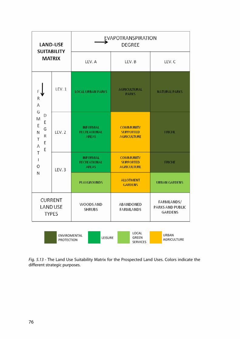
76

Fig. 5.13 - The Land Use Suitability Matrix for the Prospected Land Uses. Colors indicate the different strategic purposes.

ENVIROMENTAL

PROTECTION LEISURE LOCAL

GREEN

SERVICES

URBAN

AGRICULTURE

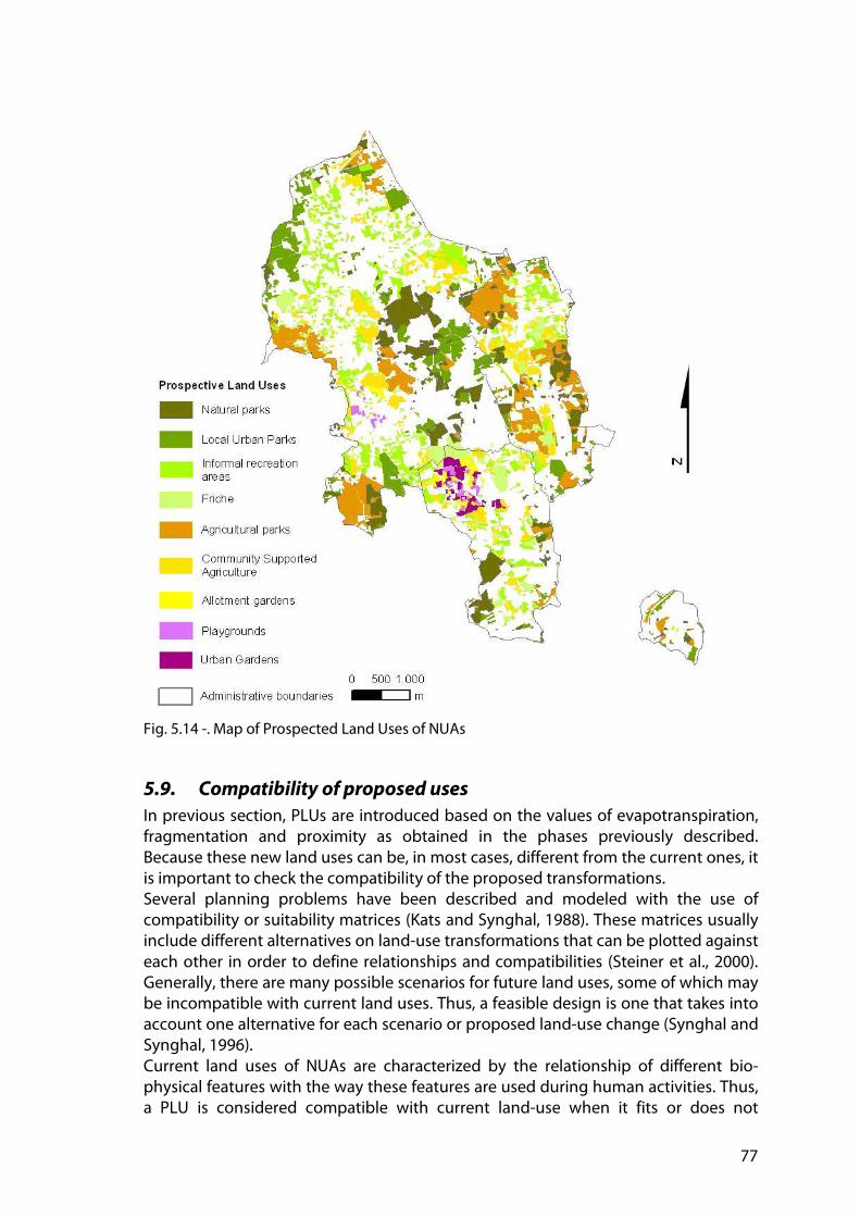
77

Fig. 5.14 -. Map of Prospected Land Uses of NUAs

5.9. Compatibility of proposed uses

In previous section, PLUs are introduced based on the values of evapotranspiration, fragmentation and proximity as obtained in the phases previously described. Because these new land uses can be, in most cases, different from the current ones, it is important to check the compatibility of the proposed transformations. Several planning problems have been described and modeled with the use of compatibility or suitability matrices (Kats and Synghal, 1988). These matrices usually include different alternatives on land-use transformations that can be plotted against each other in order to define relationships and compatibilities (Steiner et al., 2000). Generally, there are many possible scenarios for future land uses, some of which may be incompatible with current land uses. Thus, a feasible design is one that takes into account one alternative for each scenario or proposed land-use change (Synghal and Synghal, 1996). Current land uses of NUAs are characterized by the relationship of different bio-physical features with the way these features are used during human activities. Thus, a PLU is considered compatible with current land-use when it fits or does not

78

contrast with this relationship. For instance, the transformation of farmlands into another land-use that is not directly related to agricultural purposes (i.e. Natural

parks) is not compatible because it would alter the characteristics of the land cover and generate some loss of agricultural values. On the other hand, changes of farmlands to other forms of agricultural land uses (i.e., Community supported

agriculture) are considered to be compatible. In our approach, a Compatibility Matrix (Fig. 5.15) is used to check the compatibility of current land uses and PLUs. For each current land-use of the NUAs (wood and shrubs, abandoned farmlands, parks and public gardens and farmlands), the compatible PLUs are represented by solid colored boxes within the matrix. On the other side, the empty boxes indicate incompatible transformations: i.e., local urban parks or urban green spaces are not compatible with current or abandoned farmlands. Woods and shrubs are compatible with PLUs aimed at environmental protection and leisure (Natural parks, Friche, Local urban parks, Informal recreation area and Urban

gardens, Playgrounds). Abandoned farmlands and Farmlands are compatible with urban agriculture uses (Agricultural parks, Community supported agriculture and Allotment gardens). Parks and public gardens are compatible with uses for environmental protection, leisure and urban green services (Natural parks, Local urban parks, Informal recreational area and Urban gardens).

Fig. 5.15 – The compatibility matrix

ENVIROMENTAL

PROTECTION LEISURE LOCAL

GREEN

SERVICES

URBAN

AGRICULTURE

79

As already stated, the role of the Compatibility Matrix is to check the compatibility of PLUs with current land uses (Fig. 5.15). The PLUs corresponding to Lev. A and Lev. B of evapotranspiration in the land-use suitability matrix were confirmed to be compatible with current land uses, which are woods and shrubs and abandoned farmland. With Lev. C of evapotranspiration, the following cases occured: The current farmlands were not compatible with PLUs (Natural parks, Friche, and Urban gardens). In this case, the related patches may be suitable for prospective land uses that are suited to the lower level of evapotranspiration (Lev. B). These PLUs are Agricultural parks, CSA and Allotment gardens. The current parks and public gardens were compatible with Natural parks and Urban

gardens, but were not compatible with Friche. In this case, the related patches may be suitable for prospective land uses that are suited to the lower level of evapotranspiration (Lev. B). This PLU is CSA, which is also not compatible with parks and public gardens. For this reason, a PLU with Lev. A of evapotranspiration was chosen (Informal recreational areas). In general, when a current land-use was not compatible with a PLU, the alternative could be chosen among other PLUs that have the same fragmentation level. The final PLUs are mapped in Fig. 9 and summarized in Table 5. The most frequent PLU was Informal recreational areas, with 378 patches and an area of 246 ha, which corresponds to 20% of the total NUAs area. CSA followed with 331 patches and 307 ha (25%). This PLU comprised the largest total area, but displayed high fragmentation (1.43). Agricultural parks had the largest average patch area (almost 3 ha) and a high total area (263 ha, 21%). Local urban parks and Natural parks presented similar features in terms of total area (211 and 185 ha, respectively), number of patches (217 and 190) and almost the same average area (about 1 ha). Friche were characterized by a low number of patches (16) and the lowest average area (0.2 ha). Playgrounds featured 27 patches and very high fragmentation and proximity degrees (1.42 and 41.91, respectively). Allotment gardens showed the lowest number of patches (15), the highest proximity degree (43.66) and a high average area (1.3 ha).

80

Fig. 5.16 - Final map of Prospected Land Uses of NUAs after the compatibility matrix check. Table 5.5 - Statistics for Prospected Land Uses

Prospected Land

Uses (PLUs)

Number

of

patches

% num

of

Patches

Total

Area (ha)

%

are

a

Average

Patch Area

(ha)

ET FR PD

Agricultural Park 88 0.07 263.625 0.21 29957.3864 80.3 1.1611 34.0

FRICHE 16 0.01 3.7333 0.00 2333.3125 83.8 1.3077 39.6

LUP 217 0.17 210.97 0.17 9722.1198 70.9 1.1731 33.3

Natural Park 190 0.15 184.8221 0.15 9727.4789 85.4 1.1781 37.3

Playgrounds 27 0.02 11.5051 0.01 4261.1481 70.9 1.4244 41.9

Allotment Gardens 15 0.01 18.9961 0.02 12664.0667 80.3 1.4313 43.7

Informal Recreational Areas

378 0.30 246.0479 0.20 5732.2516 70.9

1.4058 29.2

CSA 331 0.26 307.2429 0.25 4736.4405 83.5 1.4278 31.8

81

5.10. An alternative method for Land Cover extraction: the R package

RasClass

Land Cover Analysis presents some limitations. Because the different land uses were geographically sampled, they were characterized by a single level of evapotranspiration. For this reason, different patches of the same land-use feature the same evapotranspiration level. This may be sufficient for larger scale characterization (metropolitan or provincial level), but may be a limitation at a smaller scale (i.e., single municipalities). To overcome this limitation, an alterantive mehod for land cover extraction is proposed. It is based on an open source package for supervised land cover analysis in order to extract land covers from digital imagery. The package has been tested on the Mascalucia area.

5.7.1. Background and methodology

Remote sensing for land cover

Perhaps the most basic form of land cover analysis in remote sensing research is the land cover classification (Aplin, 2004). The classification process involves the association of spatial objects (pixels in raster approaches) within remotely sensed imagery with specific land cover classes. These classes are fixed a-priori. The results are usually the production of land cover maps or layer. A major part of research in satellite remote sensing is dedicated to the optimization of computer aided classification processes for identifying and mapping various land cover categories. A lot of different methods have been used in the last decades, as recently summarized by Lu and Weng (2007). Many authors agree on that an ideal classification approach cannot exist due to the process complexity and to the number of factors affecting classification outputs, such as the adopted classification scheme, spectral and spatial content of the imagery, the method of making class decision, and the classification unit (Mallinis and Koutias, 2008). Lot of research are currently ongoing trying to develop new classification techniques or to hybridize with older ones to different contexts. Characteristics of land cover classification in urban contexts

Urban contexts present two particular characteristics: the presence of complex arrangement of landscape features (different mixed land uses) and the need of good spatial and spectral resolution of the images to be used for land cover extraction. High resolution imagery is more valuable and appropriate for urban planning, allowing identification of covers at local or sub-communal scale (blocks, neighborhood). The use of high resolution imagery is becoming more diffuse in land cover analysis since the decreasing of their costs. Different studies have dealt with extraction of land covers from high-spatial resolution images for urban areas (Zhang, 2001; Myeong et al., 2003; Dinis et al, 2010; Myint et al., 2011). We here focus on a supervised, pixel based method for land cover extraction in an urban areas that uses high resolution orthophotos. Both texture and contextual information contained in ancillary layers were used in order to enhance the classification overall accuracy.

82

Focusing on a highly urbanized area, a very good resolution imagery was needed, in order to extract detailed urban land covers. The same set of high-resolution orthophotos used for the Land Cover in section 5.2 was used . These orthophotos were taken during summer of 2008 at an average height of 3000 m. After orthorectification, the average scale of digital photos was 1:20000, with a pixel dimension of 0.25 m and three spectral bands (red, green and blue). Orthophotos pre-processing

Due to very high number of processing pixel, computational capacities of available personal computers were not able to run the model. For this reason, the two orthophotos were first resampled from .25 m to 1 m resolution, with nearest neighbor algorithm. Orthophotos were than merged together, obtaining a single raster of 16,147,949 pixel for each spectral band. In order to obtain the spatial coincidence with the area of the municipality under study, orthophotos were clipped to the municipal boundaries. Particular care was put so to not alter spatial position of the orthophotos. They were then converted from their native ECW format to ascii format. A total of three layers were obtained, one for each spectral band.

Definition of land cover classes

The choice of classes and their number is strictly depending on the aim of the project, study area and resolution of the images (Lu and Weng, 2007). In this study, we wanted to focus on the main covers that are present in an urban context as well as to distinguish between the two main green features that can be found in our geographical context inside urban areas: tree/shrubs and herbaceous vegetation. Six land cover classes were selected (Myint et al., 2011). Trees/shrubs (TS), Herbaceous Vegetation/grass (GR), Bare soil (BS), Clear Impervious (CI), Dark Impervious (DI), Shaded areas (SH). The choice of merging together trees with shrubs is due to their spectral similarity in the study area. The different between CI and DI is related to their spectral values: the first are characterized by clear colors (e.g. roofs, pavements or other impervious surfaces close to built up areas), the latter represent dark impervious surfaces colors (e.g. street or other asphalted surfaces). This difference was needed to distinguish among different impervious surfaces which presented an high spectral variation. Shaded areas was considered as a land cover class because of their widespread presence, a common feature in urban areas and in high resolution imagery (Myeong et al., 2003).

Training and accuracy assessment sets

In any supervised classification, the aim of the training stage is to derive a representative sample of the spectral signatures of each of the chosen land cover class (Chen and Stow, 2002). Training samples are usually collected from fieldwork, or by visual inspection from the available image data (high resolution aerial photographs or satellite images). Different collection strategies are available, such as single pixel, seed, and polygon. The strategies can influence classification results, especially in applications that use fine spatial resolution image data. (Chen and Stow, 2002). When selecting a training strategy, a range of factors should be considered, (i.e. the number of pixels to be used, the effect of spatial autocorrelation, intra-image variance, time and labor costs), but it is often not feasible to satisfy all of these factors.

83

In our case, we used a small-block training data, by manually digitizing from orthophotos a number of polygons or blocks of pixels. This approach was preferred because, for spatially heterogeneous classes like in urban contexts, small-block training can better capturing spectral and spatial information (Chen and Stow, 2002). We digitized 992 polygons by choosing them with stratified random sampling. This sampling scheme made sure that sufficient samples could be taken in rare but important map classes (Congalton and Green, 2009). The digitized polygons corresponded to a total of 120158 pixel with 1 m resolution. This set of pixel was then split in two half sub-sets, one for the training phase and the other for the accuracy assessment of the different used algorithms (see section 4.7). The number of pixel for both training and accuracy assessment was higher than the number usually required for each class by the heuristic rule of 10p-30p pixels (Van Niel et al., 2005) or 50p (Congalton and Green, 2009) for each class to be classified, where p is the number of wavebands in the available image data. Texture layers

A texture can be considered as the visual impression of coarseness or smoothness caused by the variability or uniformity of image, tone, and color (Emerson et al., 1999). It represents a homogeneous patterns of pixels that cannot be sufficiently described by spectral values. Textures are also related to the frequency of tonal change on imagery and have high values when areas are heterogeneous, while low values are present in homogeneous zones of the imagery. Textural filters have been widely used in land cover classification in order to improve accuracy results by introducing textural features in the classification process. Statistical filter are usually applied to a surrounding region (moving window) of each processed pixel, in order to attribute the statistic to the pixel itself. Texture layers are frequently used in improving land cover classification accuracy and different methods have been used (Berbereglou et al., 2000; Debeir et al., 2002; Puissant et al., 2005) If the main classification goal is to minimize the number of pixels wrongly classified, the mean texture parameter should be used (Aguera et al. 2008). A smaller window size was found to be most accurate and a five by five pixel moving window was therefore utilized (Berbereglou et al., 2000). A first order statistic (standard deviation) was performed for the three spectral bands on a 6x6 pixel moving window. Contextual Layers

The contextual information is an additional information that can be derived by internal measures on the images or by using external ancillary data (Gurney, 1983). The objective of the use of contextual information is therefore to provide information for the classification that are not spectral based (verify this!). Different studies have explored the use of contextual or other ancillary data with remotely sensed imagery to increase the accuracy of land cover classification. Liu et al. (2003), for instance, introduced geophysical information such as elevation and temperature into the classification procedure, Debeir et al. (2002) included topographic features such as roads, rivers and digital terrain features (altitude, slope, orientation). Vegetation Indices are commonly used in many remote sensing applications in urban areas to enhance classification accuracy (Myeong et al. 2001; Myint et al., 2011).

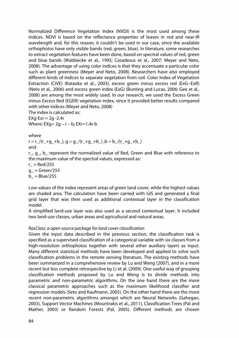
84

Normalized Difference Vegetation Index (NVDI) is the most used among these indices. NDVI is based on the reflectance properties of leaves in red and near-IR wavelength and, for this reason, it couldn’t be used in our case, since the available orthophotos have only visible bands (red, green, blue). In literature, some researches to extract vegetation features have been done, based on spectral values of red, green and blue bands (Wabbecke et al., 1995; Casadesus et al., 2007; Meyer and Neto, 2008). The advantage of using color indices is that they accentuate a particular color such as plant greenness (Meyer and Neto, 2008). Researchers have also employed different kinds of indices to separate vegetation from soil. Color Index of Vegetation Extraction (CIVE) (Kataoka et al., 2003), excess green minus excess red (ExG−ExR) (Neto et al., 2006) and excess green index (ExG) (Bunting and Lucas, 2006; Gee et al., 2008) are among the most widely used. In our research, we used the Excess Green minus Excess Red (EGER) vegetation index, since it provided better results compared with other indices (Meyer and Neto, 2008) The index is calculated as: EXg-Exr = 2g -2.4r Where: EXg= 2g – r – b; EXr=1.4r-b where r = r_/(r_+g_+b_), g = g_/(r_+g_+b_) ,b = b_/(r_+g_+b_) and r_, g_, b_ represent the normalized value of Red, Green and Blue with reference to the maximum value of the spectral values, expressed as: r_ = Red/255 g_ = Green/255 b_ = Blue/255 Low values of the index represent areas of green land cover, while the highest values are shaded area. The calculation have been carried with GIS and generated a final grid layer that was then used as additional contextual layer in the classification model. A simplified land-use layer was also used as a second contextual layer. It included two land-use classes, urban areas and agricultural and natural areas. RasClass: a open source package for land cover classification

Given the input data described in the previous section, the classification task is specified as a supervised classification of a categorical variable with six classes from a high-resolution orthophotos together with several other auxiliary layers as input. Many different statistical methods have been developed and applied to solve such classification problems in the remote sensing literature. The existing methods have been summarized in a comprehensive review by Lu and Weng (2007), and in a more recent but less complete retrospective by Li et al. (2009). One useful way of grouping classification methods proposed by Lu and Weng is to divide methods into parametric and non-parametric algorithms. On the one hand there are the more classical parametric approaches such as the maximum likelihood classifier and regression models (Seto and Kaufmann, 2005). On the other hand there are the more recent non-parametric algorithms amongst which are Neural Networks (Gahegan, 2003), Support Vector Machines (Mountrakis et al., 2011), Classification Trees (Pal and Mather, 2003) or Random Forests (Pal, 2005). Different methods are chosen

85

depending on the scope of the analysis, the extent and spatial resolution of the data and the available tools for classification (Lu and Weng, 2007). Most studies use remote sensing images to perform pixel-based classification on a single scale, but recent developments include context variables that take information from neighbouring pixels or from vectorized data into account and integrate data at multiple scales (Li et al., 2009). With increased availability of computational power and more sophisticated software tools, the trend goes away from simple parametric approaches towards increasingly complex machine learning algorithms (Gahegan, 2003; Rogan et al., 2008). In the present analysis, three state of the art, non-parametric algorithms are compared with two more classical parametric approaches. The parametric algorithms are the Maximum Likelihood Classifier and Multinomial Logistic Regression, whereas the non-parametric algorithms are Neural Networks, Support Vector Machines and Random Forests. The classification is performed by using the software package rasclass (Wiesmann and Quinn, 2011), an extension for the open source statistical programming environment R (R Development Core Team, 2011). The package rasclass facilitates the use of R classification of categorical data from raster images by combining several algorithms from other R packages specifically for raster image classification. It is fully documented and can be readily installed from within R or alternatively downloaded from the Comprehensive R Archive Network repository (CRAN). The the algorithms used in this study and their respective implementations in R are summarized in Table 5.6. Table 5.6 - Classication algorithms currently implemented in the R package rasclass

Although the statistical software R is freely available and has extensions that cover many of the currently existing classification algorithms, the software has only found little applications for land cover classification in the literature. One notable exception is a recent paper by Brenning (2009), comparing eleven different classification techniques for binomial data available in R. Brenning’s study shows the potential of using R for the purpose of land cover classification. Its modular structure allows to integrate the latest classification algorithms that are implemented in different packages in R and that will possibly be added in the future. It therefore enables the user to test several classification techniques within the same framework and to benchmark them against each other. This allows to build a raster image classification system that stays up do date and can also be extended by the user. The open source nature of R is another important feature, as it ensures full comparability and reproducibility of results and thus transparency concerning the methods applied. All analysis presented in this study has been performed using R version 2.14.0 and the package extension rasclass version 0.2.1, which builds on several other packages containing classification algorithms. The specific properties of the packages and

86

algorithms will only be described superficially here. For a more rigorous description, the reader is referred to further readings from the literature and the corresponding package documentations that are available for each algorithm. Accuracy assessment

A rigorous accuracy assessment forms an important part of any land cover mapping effort, specially when comparing different algorithms and data configurations. Standard accuracy measures from multinomial classification methods are the confusion matrix, the producer and consumer accuracies as well as the overall accuracy and its chance-corrected analogue, the kappa coefficient (Janssen and van der Wel, 1994). Although these measures are standard in the literature and will also be used here for the accuracy assessment, they have their specific advantages and disadvantages and have to be interpreted with some care (Foody, 2002). For instance, some classification algorithms might to over-fit to the given input data and so the accuracy assessment might overestimate the quality of the final map (Brenning, 2009). To address these problems and to achieve a realistic estimate of classification accuracies, a in-sample validation is performed. For this, the sample data is split into two halves, where one half is used to train the models and the other half is used to test the prediction accuracy. By splitting the data in two parts and testing the models with the part that was not previously used for training, a more realistic and more conservative estimate of the accuracy of the analysis is obtained (Brenning, 2009). The accuracy matrices as well as the derived indices are calculated from the output of 100 iterations of this validation procedure. The resulting mean and standard deviations are derived to detect statistically significant differences between algorithms and data configurations

5.7.2. Results

Accuracy assessment

The combination of the five algorithms that are compared in this analysis, together with the described configurations of input layers, resulted in the production of twenty-five different land cover maps of the study area. The overall accuracies and the k-coefficients of all twenty-five tested combinations for both the final maps and the in-sample verification are presented in fig. 5.17. The distributions of both accuracy measures resulting from the verification procedure are illustrated with box-plots in the same figure. The boxes and lines indicate the first and second quantiles respectively. Furthermore, the numerical values of the overall accuracies of the verification procedure and the final maps are given in Table 5.7.

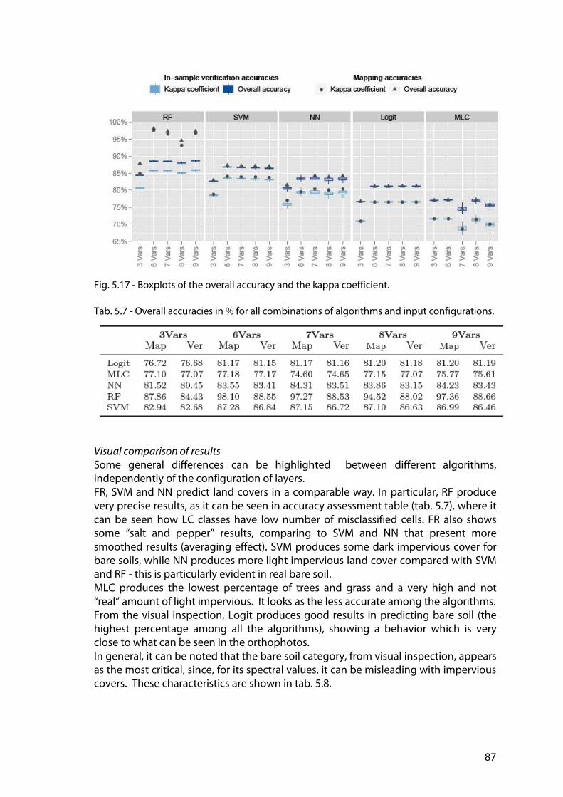
87

Fig. 5.17 - Boxplots of the overall accuracy and the kappa coefficient. Tab. 5.7 - Overall accuracies in % for all combinations of algorithms and input configurations.

Visual comparison of results

Some general differences can be highlighted between different algorithms, independently of the configuration of layers. FR, SVM and NN predict land covers in a comparable way. In particular, RF produce very precise results, as it can be seen in accuracy assessment table (tab. 5.7), where it can be seen how LC classes have low number of misclassified cells. FR also shows some “salt and pepper” results, comparing to SVM and NN that present more smoothed results (averaging effect). SVM produces some dark impervious cover for bare soils, while NN produces more light impervious land cover compared with SVM and RF - this is particularly evident in real bare soil. MLC produces the lowest percentage of trees and grass and a very high and not “real” amount of light impervious. It looks as the less accurate among the algorithms. From the visual inspection, Logit produces good results in predicting bare soil (the highest percentage among all the algorithms), showing a behavior which is very close to what can be seen in the orthophotos. In general, it can be noted that the bare soil category, from visual inspection, appears as the most critical, since, for its spectral values, it can be misleading with impervious covers. These characteristics are shown in tab. 5.8.

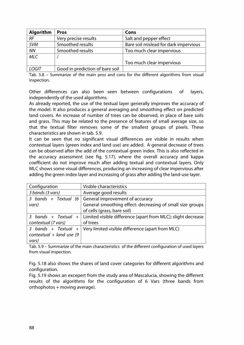
88

Algorithm Pros Cons

RF Very precise results Salt and pepper effect SVM Smoothed results Bare soil mislead for dark impervious NN Smoothed results Too much clear impervious MLC /

Too much clear impervious LOGIT Good in prediction of bare soil Tab. 5.8 – Summarize of the main pros and cons for the different algorithms from visual inspection. Other differences can also been seen between configurations of layers, independently of the used algorithms. As already reported, the use of the textual layer generally improves the accuracy of the model. It also produces a general averaging and smoothing effect on predicted land covers. An increase of number of trees can be observed, in place of bare soils and grass. This may be related to the presence of features of small average size, so that the textual filter removes some of the smallest groups of pixels. These characteristics are shown in tab. 5.9. It can be seen that no significant visual differences are visible in results when contextual layers (green index and land use) are added. A general decrease of trees can be observed after the add of the contextual green index. This is also reflected in the accuracy assessment (see fig. 5.17), where the overall accuracy and kappa coefficient do not improve much after adding textual and contextual layers. Only MLC shows some visual differences, producing an increasing of clear impervious after adding the green index layer and increasing of grass after adding the land-use layer. Configuration Visible characteristics 3 bands (3 vars) Average good results 3 bands + Textual (6

vars)

General improvement of accuracy General smoothing effect: decreasing of small size groups of cells (grass, bare soil)

3 bands + Textual +

contextual (7 vars)

Limited visible difference (apart from MLC); slight decrease of trees

3 bands + Textual +

contextual + land use (9

vars)

Very limited visible difference (apart from MLC)

Tab. 5.9 – Summarize of the main characteristics of the different configuration of used layers from visual inspection. Fig. 5.18 also shows the shares of land cover categories for different algorithms and configuration. Fig. 5.19 shows an excepert from the study area of Mascalucia, showing the different results of the algorithms for the configuration of 6 Vars (three bands from orthophotos + moving average).

89

Fig. 5.19. Shares of land use categories for di_erent algorithms and configurations

90

Fig. 5.19. An excerpt of the study area with results of the alghorithms for the configuration of 6 Vars

91

6. Discussions results, proposals and conclusions

Results and innovations for urban planning

In the context of Italian contemporary metropolitan areas, NUAs suffer from a wide range of pressures by urbanization process. This condition is not limited to particular areas of Italy, but it can be observed in different geographical contexts of different size from northern more developed regions to southern metropolitan areas (Sansa et al., 2010; Settis, 2011). The impact and externalities of these processes encompasses physical, environmental, socio-economical and political issues (EEA, 2006; Sansa et al., 2010). Particularly, in the Catania metropolitan area, NUAs have always been targeted by urban plans as generic farmlands or undefined green spaces without a particular importance or role. This has been one of the reasons why agricultural and green spaces have been continuously eroded by urban sprawl. Weak environmental policies have been one of the results of the lack of attention to NUAs. For this reason, the characterization of NUAs within urban planning is fundamental for the conservation of urban ecosystem services. Urban planning strategies for NUAs should be related to the urban surroundings (Hostetler et al., 2011) Therefore, metropolitan areas appear to be the most appropriate scale for addressing new land uses. Moreover, preserving the components of peri-urban ecosystems, such as landscape aesthetics and recreational uses, is also important, because they provide more intangible services than other ecosystems (Vejre et al., 2010)., The importance of the proposed method For urban planning is that it integrates different analytical and evaluating phases to define a new scenario of land uses for NUAs. These analytical phases come from different scientific fields (ecology, remote sensing, GIScience) but can be integrated together like a PSS an overall system so to provide information about particular features of NUAs that can be useful to understand in order to build a new scenario for their conservation. Moreover, the method, as structured, can be expanded and enriched with other analytical phases. These have to be chosen in order to include new features of NUAs (i.e. soil permeability, vegetation richness and rarity, …). Another important feature of the method that has to be underlined is that the PLUs, are always compared to the actual land uses present in the study area. The method can also be a tool for enhancing the current land-use asset, because the proposed scenario may improve the overall provision of ecosystem services in the area. In this approach, PLUs have been chosen according to four strategic categories (see section 5.5) that need to be deeply rooted in sound protection and development planning scenarios. Nevertheless, the method is not context-dependent; the categories of land-use, land cover or PLUs have been defined without further specification (i.e., type of crops in farmlands) and can therefore be used in other geographical contexts. PLUs provide a highly differentiated picture of a new spatial configuration of NUAs. Urban plans for NUAs must be developed “within the fuzzy framework of an open space network which is dynamic in aesthetic and ecological status, allowing for a larger mosaic, a patchwork of changing, loose-fit landscapes” (Thompson, 2002). This means that urban plans, at local or metropolitan scale, have the chance to choose

92

among different possibilities of new land uses and policies. This can be very important, especially for the small local municipalities that have restricted financial resources for projects on green areas. Integrating the different functions of NUAs requires governments to play a facilitating role in education and empowering change and innovation among developers/builders and residents. In particular, planners can help to identify policies to impact the design and management of proposed and existing developments that are located near NUAs. Guidelines for urban ecological networks

Finally, some considerations and guidelines can be proposed about how to design connections among NUAs for creating an urban ecological network in metropolitan areas. The development of these networks is increasingly considered a sound approach to improve the ecological value of urban greenspaces. It includes the protection of existing green spaces, creation of new spatial forms, and restoration and maintenance of connectivity among diverse green spaces (Kong et al., 2010). To maintain or restore connectivity, planners must identify the best habitat and potential corridors by considering distances and the obstacles between patches posed by the different land uses. However, in urban-contexts, some more site specific guidelines or principle can be defined, to better anchor network design to geographical context and community needs. These principles are important, as current researches have been more focused on more natural contexts (natural parks, reserves) than the metropolitan areas. With reference to the link/hub conception of ecological network the following criteria may be applied in urban context.

• Nodes/hubs must have different purposes in the ecological network.This is particularly relevant in urban areas, where a network may have different strategic purposes, from nature protection to leisure. The connection of hub for species is only one of the aims of the network

• Not every node/hub can be connected: it is not reliable to think that it is possible to connect every hub or core areas. This would result in the concrete possibility of having hubs isolated inside the urban context. For these hubs purposes of leisure and urban greenspaces should be proposed.

• Not every node/hub can be connected at the same way. According to the multifunctional purpose of an urban ecological network, the nature of connections may be highly differentiated. Connections may include agricultural or wood areas for connection of habitat purposes or urban streets for connection of urban greenspaces or areas for leisure.

• With reference to the previous points, some types of land-use can act as obstacles for some link, but cannot for others. I.e. a street may not allow the linking between two natural areas, but can be used as link for two small urban playgrounds or leisure areas

• According to the compatibility matrix introduced in the section 5.6, not every land-use may be changed to allow connections between NUAS. I.e productive or high quality farmland can be hardly changed to natural area.

In order to better define the role of hubs and links/connections in the network, it is fundamental that the rules previously outlined are embedded in the overall characterization of NUAs, in order to attribute to each NUA a differentiated nature.

93

GIS-based network design model (Zhang and Wang, 2006; Chang et al., 2011;Teng et al., 2011) can be then use to assess the efficiency of the network. Limitations and possible improvements

Land Cover Analysis presents some limitations. Because the different land uses were geographically sampled, they were characterized by a single level of evapotranspiration. For this reason, different patches of the same land-use were characterized by the same evapotranspiration level. This may be sufficient for larger scale characterization (metropolitan or provincial level), but may be a limitation at a smaller scale (i.e., single municipalities). Remote sensing techniques for land cover extraction may therefore be used (Lu and Weng, 2007). The use of the proposed supervised classification with the rasclass packacge (see section 5.7) and the use of digital high-resolution orthophotos will help to overcome this limitation and will produce differentiated land cover maps. In Proximity Analysis, more accurate results may be derived by using a network distance rather than a Euclidean one. In general, the results from the different phases were dependent on the classes of values that were used in the definition of the levels of fragmentation, evapotranspiration and proximity. An equal interval method was chosen for classifications but a different algorithm may produce different results in terms of prospective land uses. The Proximity Analysis can also be improved by using other distance metric: since space cannot be considered as homogeneous and isotropic, slope and other physical obstacle can be considered and included in a cost-weighted distance to be used to assess the accessibility of NUAs. It may not be realistic to expect that all NUAs within a single municipality would change their current land-use according to the proposed model, because, in most cases, this would mean a significant economic effort. Moreover, different PLUs may require a different extension or number of patches in order to achieve their specific functions and provision of services. For instance, the number and area of Playgrounds and Allotment gardens indicated by the LUSM appear sufficient to provide the appropriate functions of urban green and agriculture services at a local scale. In contrast, other PLUs, such as informal recreation areas and local urban parks, present a high number of patches with a relatively large overall area. In other cases (CSA), the high number of patches and large overall area of some PLUs may be not suitable for the practical needs of the local community. Therefore, some criteria for the selections of PLUs, with a higher priority for their implementation, could be introduced. These can be:

Maximization of ecosystem services provision. This aspect involves the value assessment of different existing ecosystem services, which depends upon the views and needs of stakeholders (Vermeulen and Koziell, 2002). GIS mapping approaches that define and evaluate services for each PLU could be useful (Chen et al., 2009). Different scenarios may be assessed based on the economic resources that are needed to achieve land transformations. For this reason, more sophisticated approaches than ecosystem mapping or spatial visualization may be required (Herzig, 2008).

Accessibility and spatial equity. Different PLUs need to be equally spatially distributed over the entire study area. For instance, the European Environment Agency (EEA)

94

recommends that people should have access to green spaces within 15 minutes walking distance (Barbosa et al., 2007). But this is not always true and cities often present a highly differentiated degree of accessibility to urban green spaces, especially in some southern European regions, such as Sicily. Different approaches to measure spatial equity, based on distance metrics (Talen and Anselin, 1998) or other GIS network analysis (Oh and Jeong, 2007), may be introduced.

Economic feasibility of NUAs protection. There is a wide consensus on the idea that that urban planning and open space preservation are parts of the same process (Hollis and Fulton, 2002). Even if public acquisition of land and regulatory approaches are mostly carried out for the primary purpose of protecting open space, they are often economically unsustainable for local governments. In addition this action encounters and face resistance from private landowners (Bengston et al., 2004). The issue of economic feasibility could be addressed through incentive-based approaches for managing urban growth and protecting open space (Stoms et al., 2009). From this perspective, Transfer of Development Rights programs can be used in order to protect NUAs obtaining economic benefits for different stakeholders, including the following: landowners of parcels to be protected from development; developers of parcels to be developed; and local administrations that may implement the land-use allocation decisions with no financial efforts (Brabec and Smith, 2002; Kaplowitz, 2008). Conclusions

A new compact rural -urban aimed aimed at the sustainable provision of ecosystem services should be pursued by urban planning (Magnaghi and Fanfani, 2010; Gutman, 2007). “In this new rural–urban compact there would be more employment opportunities and more income coming to the rural areas, and the cities would benefit from a sustainable supply of rural products and ecosystem services provided by restored rural environments” (Gutman, 2009). This may lead to the end of the undifferentiated use of peri-urban land, opening new perspective for the integration of urban and non-urban land uses. Some principles to underpin this new compact rural-urban can be identified:

• new forms of agriculture have to be funded and promoted by public administration, aimed at different purposes (direct provision of agricultural products to the metropolitan area, community supported agriculture, urban agricultural, agricultural park).

• Quality of the goods, short selling chain of local market should be the distinctive trademarks of the new agriculture.

• The limits of urban areas should have to be clearly defined for reducing soil consumption due to urbanization processes; this would also result in a regeneration of peri-urban space, preserving agricultural and natural areas.

• A network of peri-urban greenways should be designed among the NUAs of metropolitan areas.

With regards of the previous points, particularly important is the engagement and participation of urban population in agriculture. This concept of civic agriculture, derived from the sociology of agriculture, specifically from research on local, community-based food systems (Lyson, 2004; Goldeberger, 2011). “Embedding of

95

local agricultural and food production in the community” (Lyson, 2004:), civic agriculture represents the antithesis of the dominant large-scale, capital-intensive, industrialized agricultural system. It includes farmers markets, community supported agriculture, community and school gardens, farm stands, u-pick operations, on-farm processing, and grower-controlled marketing cooperatives. Citizen participation in agriculture is a “cornerstone” of civic agriculture and according to Lyson (2004) can transform urban citizens into “food citizens”, persons that are aware in how and where his or her food is produced, processed, and sold. This can process of public awareness is extremely important, since it can increase overall civic welfare and promote long-term sustainability

NUAs play a strategic role in the provision of ecosystem services, especially in urban metropolitan areas, where these services have become reduced both in their quantity and quality. Scenarios for land-use should be carefully planned because of the environmental, social, economic and cultural benefits that are derived from the ecosystem services provided by agriculture and green infrastructure. In the present work, the characterization of NUAs with appropriate analytical tools is therefore a fundamental step to identify their peculiarities and potentialities and to better choose the most appropriate land uses to maintain their integrity and provided ecosystem services. LCA, FA and PA, combined in a LUSM, can provide useful information and quantitative data about the choice of new land uses for NUAs and can increase the clarity and objectivity of the decision process. LCA was used to assess the different vegetation cover of NUAs, providing a measure of evapotranspiration. FA was used to evaluate the fragmentation of NUAs in terms of patch dimension and patch density. PA evaluated the proximity of residential area to NUAs, in order to quantify the number of people that have access to NUAs. PLUs were identified by a Land-Use Suitability Matrix, and their compatibility with the current land uses was ultimately checked with a Compatibility Matrix. The results showed a new spatial configuration of NUAs, which featured a highly differentiated scenario of new land uses. This scenario will give municipalities or other metropolitan public bodies (provinces, metropolitan areas) a varied range of possibilities for the implementation of planning policies on NUAs. These policies are all aimed at the conservation and increased provision of ecosystem services. This is extremely relevant in the Catania metropolitan area, where NUAs have suffered from urban sprawl and have always been considered as generic farmlands or undefined urban green spaces. The proposed method is, however, only the beginning of a planning process aimed at conservation of NUAs. Since land-use planning is a complex and long process embedded in the social end institutional framework and it is based on knowledge that is both technical and social. This knowledge is hold by different actors in the planning process and thus it needs to be communicated and transferred from one side to the other. The use of increasingly sophisticated tools and models to enrich the scientific knowledge can become highly powerful in the planning process if it is therefore part of an overall strategy of interactive involvement of social and institutional actors and of shared vision about the future of NUAs in metropolitan contexts. This is an open field for new researches in order to understand how this interaction can be pursued benefiting also from the enhancement of new technologies.

96

PSS may prove valuable tools for enhancing the role of information and knowledge in planning, thereby enabling and facilitating knowledge-based planning. For achieving this, a technocentric approach must be avoided. With many underused PSS available, focus should be put on the demand side, which is the planning community. Researches for the enhancing of PSS must follow the combined interests of communities instead of only pushing forward the a software development which is often un-linked to planner’s real needs.

97

Acknowledgements

I would like to thank the following persons which have contributed to my work and research during these years:

Professors Paolo La Greca and Francesco Martinico for their continuous help and (scientific and economic) support.

Riccardo Privitera for sharing ideas and substantial contribute on the develop of methodology.

Daniel Wiesmann for his original work on the rasclass package for land cover analysis.

Professor Giusepp Dato, for having been the father and coordinator of our doctorate school of “Analisi, Pianificazione e Gestione integrate del territorio “.

98

99

References

Green Infrastructure and Ecosystem services Boyd, J., Banzhaf, S., 2007. What are the ecosystem services? The need for standardized

environmental accounting units. Ecological Economics 63, 616- 626. Bolund P., Hunhammar S., 1999, Ecosystem services in urban areas, Ecological Economics

,29, 293–30. Bowler, D.E., Buyung-Ali, L., Knight, T.M., Pullin, A.S., 2010. Urban greening to cool towns and

cities: A systematic review of the empirical evidence. Landscape and Urban Planning 97, 147-155.

Brown, T.C., Bergstrom, J.C., Loomis, J.B., 2007. Defining, valuing and providing ecosystem goods and services. Natural Resources Journal 47, 329-376.

Conservation Fund, 2000. Welcome to the GreenInfrastructure.Net Website: Providing a Strategic Framework for Smart Conservation. Online: available at http://greeninfrastructure.net/. Last access: November, 11, 2011.

Costanza, R., d’Arge, R., de Groot, R., Farber, S., Grasso, M., Hannon, B., Limburg, K., Naeem, S., O’Neill, R., Paruelo, J., Raskin, R., Sutton, P., van den Belt, M., 1997. The value of the world’s ecosystem services and natural capital. Nature 387, 252–259.

Daily, G. (ed) 1997. Nature's Services: Societal Dependence on Natural Ecosystems, Island Press, Washington DC.

de Groot, R.S., Wilson, M.A., Boumans, R.M.J., 2002. A typology for the classification, description and valuation of ecosystem functions, goods and services. Ecological Economics 41, 393–408.

de Groot, R.S., Alkemade, R., Braat, L., Hein, L., Willemen, L., 2010. Challenges in integrating the concept of ecosystem services and values in landscape planning, management and decision making. Ecological Complexity 7, 260-272

Escobedo, F.J., Kroeger T., Wagner J.E. 2011, Urban forests and pollution mitigation: Analyzing ecosystem services and disservices, Environmental Pollution159, 2078-2087.

Fang, C.F., Ling, D.L., 2003. Investigation of the noise reduction provided by tree belts. Landscape and Urban Planning 63, 187–195.

Fisher, B., Turner, R.K., 2008. Ecosystem services: classification for valuation. Biological Conservation 141, 1167-1169.

Füssel, H.M., 2007. Adaptation Planning for Climate Change: Concepts, Assessment Approaches and Key Lessons, Sustainability Science 2, 265–275.

GLP, 2005. Science Plan and Implementation Strategy. IGBP Report No. 53/IHDP Report No. 19. IGBP Secretariat, Stockholm.

Givoni, B., 1991. Impact of planted areas on urban environmental quality: a review. Atmospheric Environment 25, 289–299.

Jo, H.K., 2002. Impacts of urban green space on offsetting carbon emissions for middle Korean. Journal of Environmental Management 64, 115–126.

Hostetler M., Allen W., Meurk C., (2011). Conserving urban biodiversity? Creating green infrastructure is only the first step .Landscape and Urban Planning 100, 369-371.

Kaplan, R., Kaplan, S., 1989. The Experience of Nature. Cambridge University Press, Cambridge.

Kong, F., Nakagoshi, N., 2006. Spatial-temporal gradient analysis of urban green spaces in Jinan, China. Landscape and Urban Planning 78, 147–164.

Kong F., Yin H., Nakagoshi N., Zong Y.,. 2010. Urban green space network development for biodiversity conservation: Identification based on graph theory and gravity modelling. Landscape and Urban Planning 95, 16–27

Kroeger, T., Casey, F., 2007. An assessment of market-based approaches to providing ecosystem services on agricultural lands. Ecological Economics 64, 321-332.

Millennium Ecosystem Assessment, 2005. Ecosystems and Human Well-Being: Current State and Trends. Island Press, Washington, DC.

100

McHale, M.R., Mc Pherson, E.G., Burke, I.C., 2007. The potential of urban tree plantings to be cost effective in carbon credit markets. Urban Forestry & Urban Greening 6, 49–60.

Miller, W., Collins, M., Steiner, F., Cook, E., 1998. An approach for greenway suitability analysis, Landscape. Landscape Urban Planning 42, 91–105.

Moore, T. (Ed.), 2002. Protecting Maryland’s Green Infrastructure: The Case for Aggressive Public Policies. Maryland Department of Natural Resources, Chesapeake and Coastal Watershed Service.

Nowak, D.J., Crane, D.E., 2002. Carbon storage and sequestration by urban trees in the USA. Environmental Pollution 116, 381–389.

Oke, T.R., 1989. The micrometerology of the urban forest. Phil. Trans. R. Soc. Lond. B. 324, 335–349.

Sandström, U.G., 2002. Green infrastructure planning in urban Sweden, Planning Practice and Research 17, 373–385.

Swinton et al., 2007,Ecosystem services and agriculture: Cultivating agricultural ecosystems for diverse benefits, Ecological Economics, 64, 245–252.

Tallis, H., Polasky, S., 2009. Mapping and valuing ecosystem services as an approach for conservation and natural resources management. The Year in Ecology and Conservation Biology: Annals of the New York Academy of Science 1162, 265-283.

Thompson, C.W., 2002. Urban open space in the 21st century. Landscape and Urban Planning 60, 59–72.

Tzoulas K., James P., 2010, Peoples’ use of, and concerns about, green space networks: A case study of Birchwood, Warrington New Town, UK, Urban Forestry & Urban Greening, 9, 121–128

Tzoulas, K., Korpela, K., Venn, S., Yli-Pelkonen, V., Kazmierczak, A., Niemela, J., James, P., 2007. Promoting ecosystems and human health using green infrastructure: A literature review. Landscape and Urban Planning 81, 167–178.

Walmsley, A., 2006. Greenways: multiplying and diversifying in the 21st century. Landscape and Urban Planning 76, 252–290.

Weber, T., Sloan, A., Wolf, J., 2006. Maryland’s Green Infrastructure Assessment: Development of a comprehensive approach to land conservation. Landscape and Urban Planning 77, 94–110.

Young R. F., 2010. Managing municipal green space for ecosystem services, Urban Forestry & Urban Greening 9, 313–321.

New forms of agriculture

Donadieu, P., 1998. Les Campagnes Urbaines. Actes Sud, Arles. Goldberger, J.R. 2011. Conventionalization, civic engagement, and the sustainability of

organic agriculture, Journal of Rural Studies, 27, 288-296. Gutman P., 2007. Ecosystem services: Foundations for a new rural-urban compact, Ecological

Economics 62, 383-387 Hovorka, A., 2005. The (re) production of gendered positionality in Botswana’s commercial

urban agriculture sector. Annals of the Association of American Geographers, 95, 294–313.

Jarosz, L., 2008. The city in the country: Growing alternative food networks in Metropolitan areas. Journal of Rural Studies 24, 231–244.

Heimlich R. E., 1989. Metropolitan Agriculture: Farming in the City's Shadow, Journal of the American Planning Association, 55, 457-466 Lyson, A., Civic Agriculture: Reconnecting Farm, Food, and Community, Tufts University

Press, Medford. Rubino, A., 2007. The allotment gardens of the Ile de France: a tool for social development.

Journal of Mediterranean Ecology 8, 67-75. Ryan, R.L., 2002. Preserving rural character in New England: local residents’ perceptions of

alternative residential development. Landscape and Urban Planning 61, 19–35.

101

UN, 1997. Urban and Rural Areas 1996. UN, New York United Nations publications (ST:ESA:SER.a:166), Sales No. E97.XIII.3, 1997.

Van En, R., 1995. Eating for your community: Towards agriculture supported community. In Context (Fall) 42, 29–31.

Wells, B.L., Gradwell, S., 2001. Gender and resource management: Community supported agriculture as caring-practice. Agriculture and Human Values 18, 107–119.

Zasada I., 2011. Multifunctional peri-urban agriculture—A review of societal demands and the provision of goods and services by farming. Land-use policy 28, 639– 648

Landscape and urban planning

Angel, S., Sheppard, C.S., Civco, L.D., 2005. The Dynamics of Global Urban Expansion. The World Bank, Washington D.C.

Antrop, M., Van Eetvelde, V., 2000. Holistic aspects of suburban landscapes: visual image interpretation and landscape metrics. Landscape and Urban Planning, 50, 43-58.

Antrop M., 2004. Landscape change and the urbanization process in Europe. Landscape and Urban Planning 67, 9–26.

Baldock D, Beaufoy, G, Bennett, G, Clark, J (1993). Nature Conservation and New Directions in the Common Agricultural Policy. Report for the Ministry of Agriculture, Nature Management and Fisheries, The Netherlands. Institute for European Environmental Policy, HPC, Arnhem. 224 p

Barbosa, O., Tratalos, J. A., Armsworth, P. R., Davies, R. G., Fuller, R. A., Johnson, P., Gaston, K. J., 2007. Who benefits from access to green space? A case study from Sheffield, UK. Landscape and Urban Planning. 83, 187-195.

Bart, I.L., 2010. Urban sprawl and climate change: A statistical exploration of cause and effect, with policy options for the EU. Land Use Policy 27, 283–292.

Beatley, T., 2000. Green Urbanism: Learning from European Cities, Island Press, Washington, DC.

Benedict, M.A., McMahon, E., 2006. Green infrastructure: linking landscapes and communities. Island Press Washington, DC.

Bengston, D.N., Fletcher, J.O., Nelson, K.C., 2004. Public policies for managing urban growth and protecting open space: policy instruments and lessons learned in the United States. Landscape and Urban Planning. 69, 271–286.

Binns, T., Lynch, K., 1998. Feeding Africa’s growing cities into the 21st century: The potential of urban agriculture. Journal of International Development, 10, 777–793.

Bowler, D.E., Buyung-Ali, L., Knight, T.M., Pullin, A.S., 2010. Urban greening to cool towns and cities: A systematic review of the empirical evidence. Landscape and Urban Planning, doi:10.1016/j.landurbplan.2010.05.006.

Bourne, L.S., 1996. Reinventing the Suburbs: Old Myths and New Realities. Progress in Planning 46, 163-184.

Brabec, E., Smith, C., 2002. Agricultural land fragmentation: the spatial effects of three land protection strategies in the eastern United States. Landscape and Urban Planning. 58, 255-268.

Calthorpe, P., 1993. The Next American Metropolis. Ecology Community and the American Dream, Princeton Architectural Press, New York.

Camagni, R., Gibelli, M. C., Rigamonti, P., 2002. Urban mobility and urban form: the social and environmental costs of different patterns of urban expansion. Ecological Economics 40, 199–216.

Carsjens, G. J., Van der Knaap, W., 2002. Strategic land-use allocation: dealing with spatial relationships and fragmentation of agriculture. Landscape and Urban Planning 58, 171–179.

Chang, H., Li, F., Li, Z., Wang, R. & Wang, Y., 2011. Urban landscape pattern design from the viewpoint of networks: A case study of Changzhou city in Southeast China, Ecological Complexity 8 , 51-59.

102

Cook E.A., 2002. Landscape structure indices for assessing urban ecological networks, Landscape and Urban Planning 58, 269-280.

Council of European Union, 1997. The Pan-European Biological and Landscape Diversity Strategy: its aims, key principles, procedures and partners. Available at http://www.coe.int/t/dg4/cultureheritage/nature/biodiversity/default_en.asp. Last access September 9, 2011.

Cutsinger, J., Galster, G., Wolman, H., Hanson, R., Towns, D., 2005. Verifying the multidimensional nature of metropolitan land use: advancing the understanding and measurement of sprawl, Journal of Urban Affairs 27, 235–259.

Dematteis, G., 1997. Globalisation and regional integration: the case of the Italian urban system, GeoJournal 43, 331–338.

Duc Uy, P., Nakagoshi, N., 2008. Application of land suitability analysis and landscape ecology to urban greenspace planning in Hanoi, Vietnam. Urban Forestry & Urban Greening 7, 25–40.

European Environmental Agency (EEA). 2006. Urban sprawl in Europe The ignored challenge. Report 10, EEA, Copenhagen.

Haughton G., Hunter C. 1994. Sustainable Cities, Regional Policy and Development, Jessica Kingsley, London

Foley, J.A., DeFries, R., Asner, G.P., Barford, C., Bonan, G., Carpenter, S.R., Chapin, F.S., Coe, M.T., Daily, G.C., Gibbs, H.K., Helkowski, J.H., Holloway, T., Howard, E.A., Kucharik, C.J., Monfreda, C., Patz, J.A., Prentice, I.C., Ramankutty, N., Snyder, P.K., 2005. Global consequences of land use. Science 309 (5734), 570–574.

Galster, G., Hanson, R., Ratcliffe, M. R., Wolman, H., Coleman, S., Freihage, J., 2001. Wrestling sprawl to the ground: defining and measuring an elusive concept. Housing Policy Debate 12, 681–717.

Gant R. L., Robinson G. M., Shahab Fazal S., 2011. Land-use change in the ‘edgelands’: Policies and pressures in London's rural–urban fringe. Land Use Policy, 28, 266-279.

Gallent N., and. Shaw D., 2007. Spatial planning, area action plans and the rural next urban fringe. Journal of Environmental Planning and Management, 50, 617–638

Gill, S.E., Handley, J. F., Ennos, A., R. Pauleit, S., Theuraya, N., Lindley, S. J., 2008. Characterising the urban environment of UK cities and towns: A template for landscape planning, Landscape and Urban Planning 87. 210–222.

Groenewegen, P.P., Berg, A.E., Vries, S., Verheij, R.A., 2006. Vitamin G: effects of green space on health, well-being, and social safety. Study Protocol, BMC Public Health 6,149.

Gurrutxaga M., Lozano PJ, del Barrio G., 2010. GIS-based approach for incorporating the connectivity of ecological networks into regional planning. Journal for Nature Conservation 18, 318-326.

Haase, D., Nuissl, H., 2007. Does urban sprawl drive changes in the water balance and policy? The case of Leipzig (Germany) 1870–2003. Landscape and Urban Planning 80, 1–13.

Handley, J., Pauleit, S., Gill, S., 2007. Landscape sustainability and the city, in: Benson, J.F., Roe, M. (Eds.), Landscape and Sustainability, 2nd ed. Routledge, London, pp. 167–195.

Heimlich, R.E., Barnard, C.H., 1992. Agricultural adaptation to urbanization: farm types in northeastmetropolitan areas. Northeastern Journal of Agricultural and Resource Economics 21, 50–60.

Hollis, L.E., Fulton, W., 2002. Open space protection: conservation meets growth management. Discussion Paper. Center on Urban and Metropolitan Policy, The Brookings Institution, Washington, DC. Available at: http://www.brookings.edu/reports/2002/04metropolitanpolicy_hollis.aspx. Last access: 07/21/2011.

Indovina, F., 1990. La città diffusa, Quaderni DAEST, Venezia Jansen, H.G.P., Bouman, B.A.M., Schipper, R.A., Hengsdijk, H., Nieuwenhuyse, A., 2005. An

interdisciplinary approach to regional land use analysis using GIS, with applications to the Atlantic Zone of Costa Rica. Agricultural Economics 32, 87–104.

103

Jim, C.Y., Chen, S.W., 2003, Comprehensive green space planning based on landscape ecology principles in compact Nanjing city, China. Landscape and Urban Planning 65, 95–116.

Johnson, M. P., 2001, Environmental impacts of urban sprawl: a survey of the literature and proposed research agenda. Environment and Planning A 33, 717–735.

Kaplowitz, M. D., Machemer, P., Pruetz, R., 2008. Planners’ experiences in managing growth using transferable development rights (TDR) in the United States. Land Use Policy. 25, 378-387.

Kasanko, M., Barredo, J. I., Lavalle, C., McCormick, N., Demicheli, L., Sagris. V., Brezger A., 2006. Are European cities becoming dispersed? A comparative analysis of 15 European urban areas. Landscape and Urban Planning 77, 111–130.

Kilic, S., Evrendilek, F., Enol, S.S., Elik, I.C., 2005. Developing a suitability index for land uses and agricultural land covers: a case study in Turkey. Environmental Monitoring and Assessment 102, 323–335.

Kochan, B., 2007. Achieving a suburban renaissance The policy challenges. Town and Country Planning Association, London.

Kühn, M., 2003. Greenbelt and Green Heart: separating and integrating landscapes in European city regions. Landscape and Urban Planning 64, 19–27.

La Greca, P., La Rosa, S.D., Martinico, F., Privitera, R., 2011. Agricultural And Green Infrastructures: The Role Of Non-Urbanised Areas For Eco-Sustainable Planning In A Metropolitan Region. Environmental Pollution 159, 2193-2202.

Magnaghi A., Fanfani D., 2010. Patto città-campagna. Un progetto di bioregione urbana per la Toscana. Alinea.

Magoni M., Steiner F., 2001. The environment in the provincial plan of Cremona, Italy. Environmental Management 27, 639-654.

Martinico F. 2005, The Clumsy Metropolis Urban Dynamics and Globalization in a Metropolitan Area of the Southern Italy”, in La Greca P. (ed), “Planning in More Globalized and Competitive World”, The Hague-Roma,, ISoCaRP – Gangemi

Martinico, F., La Rosa, D., 2009. The Use of GIS in Landscape Protection Plan in Sicily, in: Krek, A., Rumor, M., Zlatanova, S., Fendel, E. M., (Eds) Urban and Regional Data Management. UDMS Annual 2009, 325-335, CRC/Balkema, Leiden.

Martinotti G., 2000. La dimensione metropolitana. Sviluppo e governo della nuova città, Il Mulino, Bologna.

Marull, J., Pino, J., Mallarach, J.M., Cordobilla, M.J., 2007. A Land Suitability Index for Strategic Environmental Assessment in metropolitan areas. Landscape and Urban Planning 81, 200–212.

Munoz, F., 2003. Lock living: urban sprawl in Mediterranean cities. Cities 20 (6), 381–385. Newman, P., Kenworthy, J., 1996. The land use-transport connection. An Overview. Land Use

Policy, 13, 1-22. Oh, K., Jeong, S., 2007. Assessing the spatial distribution of urban parks using GIS. Landscape

and Urban Planning. 82, 25–32. Olson, R. K., Lyson, T. A , 1999, Under the Blade: The Conversion of Agricultural Landscapes, :

Westview Press, Boulder, CO.. Nuissl, H., Haase, D., Lanzendorf, M., Wittmer, H., 2009. Environmental impact assessment of

urban land use transitions. A context- sensitive approach. Land Use Policy, 26, 414-424. Peiser, R., 2001. Decomposing Urban Sprawl Town Planning Review 72, 275-298. Piccinato, G., 1993. Urban Landscapes and Spatial Planning in Industrial Districts: The Case of

Veneto. European Planning Studies 1, 181-198. Privitera R., 2010. Pianificare fra citta' e campagna urbanizzata. Il ruolo delle aree non

urbanizzate e dell'agricoltura periurbana nel contesto metropolitano catanese. Ph. D. Thesis. University of Catania.

Sanfilippo E. D. 1991, Catania, città metropolitana, Maimone, Catania. Sansa F., Garibaldi A., Massari A., Preve M., Salvaggiulo G., 2010. La Colata. Il partito del

cemento che sta cacellando l’Italia e il suo Futuro. Chiare Lettere.

104

Schetke S., Pileri P., Kötter T., Tomasini L., 2010. Counteracting sprawl and land consumption in the urban-rural interface of the European agglomerations Milan and Cologne/Bonn: framework conditions and planning approaches. Proceedings of the International Conference ‘Managing the Urban Rural Interface Strategies and Tools for Urban Development and Sustainable Peri-urban Land Use Relationships’, Copenhagen October 19 – 22, 2010.

Settis S., 2011. Paesaggio, costituzione e cemento, Einaudi, Torino (In italian) Singhal, J., Singhal, K., 1996. The number of feasible designs in a compatibility matrix,

European Journal of Operational Research 94, 186-193. Smoyer-Tomic, K.E., Hewko, J.N., Hodgson M.J., 2004. Spatial accessibility and equity of

playgrounds in Edmonton, Canada. The Canadian Geographer / Le Géographe canadien 48, 287–302.

Steiner, F., McSherry, L., Cohen, J., 2000. Land suitability analysis for the upper Gila River watershed. Landscape and Urban Planning. 50, 199–214.

Stoms, D., McDonald, J.M., Davis, F.W., 2002, Fuzzy assessment of land suitability for scientific research reserves. Environmental Management 29, 545–558.

Stoorvogel, J.J., Schipper, R.A., Jansen, D.M., 1995. USTED: a methodology for a quantitative analysis of land use scenarios, Netherlands. Journal of Agricultural Science 43, 5–18.

Talen, E., Anselin, L., 1998. Assessing spatial equity: an evaluation of measures of accessibility to public playgrounds. Environment and Planning A 30, 595–613.

Tarrant, M.C., Cordell, H.K., 2002. Amenity values of public and private forests: examining the value–attitude relationship. Journal of Environmental Management 30, 692–703.

Teng, M., Wu, C., Zhou, Z., Lord, E., Zheng, Z.. 2011, Multipurpose greenway planning for changing cities: A framework integrating priorities and a least-cost path model", Landscape and Urban Planning 103, 1-14.

Thapa, R. B., Murayama, Y., 2008. Land evaluation for peri-urban agriculture using analytical hierarchical process and geographic information system techniques: A case study of Hanoi. Land Use Policy 25, 225–239.

Thompson, A., Stalker Prokopy, L. 2009. Tracking urban sprawl: Using spatial data to inform farmland preservation policy, Land-use Policy 26, 194–202.

Thornton, A., 2007. Beyond the Metropolis: Small Town Case Studies of Urban and Peri-urban Agriculture in South Africa. Urban Forum 19, 243–262.

Travisi, C.M., Camagni, R., Nijkamp, P., 2010. Impacts of urban sprawl and commuting: a modelling study for Italy. Journal of Transport Geography 18, 382–392.

Tu, J., Xia, Z.,Clarke, K., Frei, A., 2007. Impact of Urban Sprawl on Water Quality in Eastern Massachusetts, USA. Environmental Management 40, 183–200.

Van der Ryn, S., Cowan, S., 2006. Ecological Design (10th anniversary), Island Press. Wilson, A.G., 2006. Ecological and urban systems models: some explorations of similarities in

the context of complexity theory. Environment and Planning A 38, 633–646. Whitehand,J.W.R, 1988. Urban fringe belts: development of an idea. Planning Perspectives,

3, 47-58. Yang, J., McBride, J., Zhou, J., Sun, Z., 2005. The urban forest in Beijing and its role in air

pollution reduction. Urban Forestry & Urban Greening 3, 65–78. Zhang L., Wang H. 2006. Planning an ecological network of Xiamen Island (China) using

landscape metrics and network analysis. Landscape Urban Planning 78, 449-456. Landscape Ecology

August, P., Iverson, L., Nugrad, J., 1998. Human Conversion of Terrestrial Habitats, in: Gutzwiller K.J. (Ed), Applying Landscape Ecology in Biological Conservation. Springer-Verlag, New York, pp. 198-224.

Bascompte J. 2007, Networks in Ecology, Basic and Applied Ecology 8, 485—490 Forman, R.T.T., 1995. Land Mosaics. The Ecology of Landscapes and Regions. University Press,

Cambridge.

105

Collinge, S. K., 2009. Ecology of fragmented landscapes. The Johns Hopkins University Press, Baltimore.

Krummel, J. R., R. H. Garner, G. Sugihara, R. V. O'Neill, and P. R. Coleman, 1987, Landscape patterns in a disturbed environment. Oikos 48, 321-31

Gulinck, H. & Wagendorp, T. ,2002. References for fragmentation analysis of the rural matrix in cultural landscapes, Landscape and Urban Planning,58, 137-146.

Gustafson, E. J., 1998. Quantifying Landscape Spatial Pattern: What Is the State of the Art? Ecosystems 1, pp. 143–156.

Jongman R.H.G., Kulvik M., Kristiansen I., 2004. European ecological networks and greenways. Landscape Urban Planning 68, 305–319

Jongman R., 2004. The context and concept of ecological Networks. In: Jongman R, Pungetti G (Eds.), Ecological networks and greenways. Concept and implementation. Cambridge University Press, Cambridge, pp 7–33

Margalef, R. (1991). Networks in ecology. In M. Higashi and T. P. Burns (Eds.), Theoretical studies of ecosystems – The network perspective (pp. 41–57). Cambridge: Cambridge University Press.

Riitters, K.H., O’Neil, R.V., Hunsaker, C.T., Wickham, J. D., Yankee, D. H., Timmins, S. P., Jones, K.B., Jackson, B. L., 1995. A factor analysis of landscape pattern and structure metrics. Landscape Ecology 10, 23-39.

Rutledge, D., 2003. Landscape indices as measures of the effects of fragmentation: can pattern reflect process?. Doc science int. series 98. Department of Conservation, Wellington.

Schrijnen P.J., 2000. Infrastructure networks and red-green patterns in city regions. Landscape and Urban Planning 48, 191–204.

Turner, M.G., 1989. Landscape ecology: the effect of pattern on process. Annual Review of Ecology and Systematics 20, 179-197.

Remote sensing and Land Cover analysis

Agüera, F., F.J. Aguilar, and M.A. Aguilar, 2008. Using texture analysis to improve per-pixel classification of very high resolution images for mapping plastic greenhouses, ISPRS Journal of Photogrammetry and Remote Sensing, 63, 635–646.

Aplin, P. (2004) Remote sensing: Land cover. Progress in Physical. Geography. 28, 283-293. Akbari, H., Rose, L.S., Taha, H., 2003. Analyzing the land cover of an urban environment using

high-resolution orthophotos. Landscape and Urban Planning 63, 1-14. Brenning, A. (2009). Benchmarking classifiers to optimally integrate terrain analysis and

multispectral remote sensing in automatic rock glacier detection. Remote Sensing of Environment 113,239-247.

Casadesus et al. 2007 Using vegetation indices derived from conventional digital camera as selection criteria for wheat breeding in water-limited environments. Annals of Applied Biology 150, pp. 227–236

Cihlar, J., & Jansen, L.J.M. 2001. From land cover to land-use: a methodology for efficient land-use mapping over large areas. The Professional Geographer, 53(2).

Comber A. J. 2008 .The separation of land cover from land use using data primitives. Journal of Land Use Science, 4 (3).

Congalton, R. G., Green, K., 2009. Assessing the accuracy of remotely sensed data: principles and practices. CRC Press, 2nd ed. Boca Raton, FL.

Debeir, O., Van den Steen, I., Latinne, P., Van Ham, P. and Wolff, E. 2002: Textural and contextual land-cover classification using single and multiple classifier systems. Photogrammetric Engineering and Remote Sensing 68, 597–605.

Dinis J., Navarro A., Soares F. , Santos T., Freire S., Fonseca A., Afonso N., Tenedório J. 2010 hierarchical object-based classification of dense urban areas by integrating high spatial resolution satellite images and lidar elevation data, In Addink, E.A. and F.M.B. Van Coillie

106

(Eds). 2010. GEOBIA 2010-Geographic Object-Based Image Analysis. Ghent University, Ghent, Belgium, 29 June – 2 July. ISPRS Vol.No. XXXVIII-4/C7, Archives ISSN No 1682-1777

Endreny, T.A., 2006. Land Use and Land Cover Effects on Runoff Processes: Urban and Suburban Development, in Encyclopedia of Hydrological Sciences, M. G. Anderson ed, John Wiley & Sons, Chichester, pp. 1775-1804, 2005.

Fisher, P.F., Comber, A.J., Wadsworth, R.A. 2005. Land use and Land cover: Contradiction or Complement. In Fisher, P., Unwin, D., (Ed.), Re-Presenting GIS, Chichester, UK: Wiley

Foody, G. M. (2002). Status of land cover classification accuracy assessment. Remote Sensing of Environment 80,185-201.

Emerson, Ch., N. Siu-Ngan Lam, and D.A. Quattrochi, 1999. Multiscale fractal analysis of image texture and pattern. Photogmmmetric Engineering & Remote Sensing, 65(1):51-61.

Gahegan, M. (2003). Is inductive machine learning just another wild goose (or might it lay the golden egg)? International Journal of Geographical Information Science, 17(1):69-

Goonetilleke A., Thomas E., Ginn S., Gilbert S.(2005). Understanding the role of land use in urban stormwater quality management, Journal of Environmental Management 74, 31–42

Janssen, L. F. and van derWel, F. J. M. (1994). Accuracy assessment of satellite derived land-cover data: A review. Photogrammetric Engineering and Remote Sensing, 60(4), 419-426.

Herold, M., X. Liu, and K.C. Clarke, 2003. Spatial metrics and image texture for mapping urban land-use, Photogrammetric Engineering & Remote Sensing, 69(9):991–1001.

U. Kanjir, T. Veljanovski, A. Marsetič, K. Oštir, 2010, Application of object based approach to heterogeneous land cover/use. In Addink, E.A. and F.M.B. Van Coillie (Eds). 2010. GEOBIA 2010-Geographic Object-Based Image Analysis. Ghent University, Ghent, Belgium, 29 June – 2 July. ISPRS Vol.No. XXXVIII-4/C7, Archives ISSN No 1682-1777

Li, Y., Yan, L., and Liu, J. (2009). Remote sensing image classification development in the past decade. In Udupa, J. K., Sang, N., Nyul, L. G., and Tong, H., editors, MIPPR 2009: Multispectral Image Acquisition and Processing, volume 7494, pages 74941D{6, Yichang, China. SPIE.

Liu, J.Y., Zhuang, D.F., Luo, D. and Xiao, X. 2003: Land-cover classification of China: integrated analysis of AVHRR imagery and geophysical data. International Journal of Remote Sensing 24, 2485–500.

Lu, D., Weng, Q. 2007 A survey of image classification methods and techniques for improving classification performance. Int. J. Remote Sens., 28, 823-870.

Lu, D., Hetrick S., Moran E., Land Cover Classification in a Complex Urban-Rural Landscape with QuickBird Imagery. 2010, Photogrammetric Engineering & Remote Sensing, Vol. 76, No. 10, pp. 1159–1168.

Mallinis G., Koutias N (2008). Spectral and Spatial-Based Classification for Broad-Scale Land Cover Mapping Based on Logistic Regression. Sensors 8, 8067-8085; DOI: 10.3390/s8128067

Mountrakis, G., Im, J., and Ogole, C. (2011). Support vector machines in remote sensing: A review. ISPRS Journal of Photogrammetry and Remote Sensing, 66(3):247-259

Myeong S., Nowak D. J., Hopkins P.F. and Brock R. H., 2001. Urban cover mapping using digital, high-spatial resolution aerial imagery, Urban Ecosystems, vol. 5, pp. 243-256.

Myint, S.W., Gober P., Brazel A., Grossman-Clarke S., Weng Q., 2011.Per-pixel vs. object-based classification of urban land cover extraction using high spatial resolution imagery, Remote Sensing of Environment, doi:10.1016/j.rse.2010.12.017

Pal, M. and Mather, P. M. (2003). An assessment of the effectiveness of decision tree methods for land cover classification. Remote Sensing of Environment, 86(4):554{565.

Pal, M. (2005). Random forest classifier for remote sensing classification. Inter- national Journal of Remote Sensing, 26(1), 217-222.

Puissant A. Hirsch J., Weber C., 2005. The utility of texture analysis to improve per-pixel classification for high to very high spatial resolution imagery. International Journal of Remote Sensing, Vol. 26., 4., 733—745

107

R Development Core Team (2011). R: A Language and Environment for Statistical Computing. R Foundation for Statistical Computing, Vienna, Austria.

Rogan, J., Franklin, J., Stow, D., Miller, J., Woodcock, C., and Roberts, D. (2008). Mapping land-cover modifications over large areas: A comparison of machine learning algorithms. Remote Sensing of Environment, 112(5), 2272-2283.

Seto, K. C. . and Kaufmann, R. K. . (2005). Using logit models to classify land cover and land-cover change from landsat thematic mapper. International Journal of Remote Sensing, 26, 563-577.

Tappan, G.G., Sall, M., Wood, E. C., Cushing, M., 2004. Ecoregions and land cover trends in Senegal, Journal of Arid Environments 59, 427-462.

T.G. Van Niel, T.R. McVicar and B. Datt, (2005), On the relationship between previous termtrainingnext term sample previous termsize and data dimensionality of broadband multi-temporal classification. Remote Sensing of Environment 98, 468–480.

Wiesmann, D. and Quinn, D. (2011). rasclass: Supervised Raster Image Classification. R package version 0.1.

Woebbecke, D.M., Meyer, G.E., B.K., V., Mortensen, D.A., 1995a. Color indices for weed identification under various soil, residue and lighting conditions. Transactions of the ASAE 38, 259–269.

Zhang, Y. (2001) Texture-integrated classification of urban treed areas in high-resolution color-infrared imagery. Photogrammetric Engineering and Remote Sensing 67, 1359–1365.

Geographical Information Science

Bartlett, J.E., Kotrilk, J., Higgins, C., 2001. Organizational Research: Determining Appropriate Sample Size in Survey Research Information Technology. Learning and Performance Journal 19, 43-50.

Frank, A. U., 1992. Qualitative spatial reasoning about distances and directions in geographic space. Journal of Visual Languages and Computing 3: 343–71

Geertman, S.C.M., Ritsema Van Eck, J.R., 1995. GIS and models of accessibility potential: an application in planning. International Journal of Geographical Information Science 9, 67–80.

Herzig, A., 2008. A GIS-based Module for the Multiobjective Optimization of Areal Resource Allocation, 11th AGILE International Conference on Geographic Information Science 2008 University of Girona, Spain. Available at http://plone.itc.nl/agile_old/Conference/2008-Girona/index.htm. Last access: 07/21/2011.

Katz, J.L., Singhal, J., 1988. Structural properties of the compatibility matrix: Existence of mathematical relationships, Infor 26(3), 163-169.

Liu, H, Wang, Y., Zhang, X., 1999. Effect of spatial measurement unit on calculation of landscape indices. Geoinformatics and Socioinformatics. The Proceedings of Geoinformatics '99 Conference.

Openshaw, S., Taylor, P.J., 1981. The modifiable areal unit problem, in: Wrigley, N., Bennett, R.J. (eds.), Quantitative Geography: A British View. Routledge and Kegan, London, pp. 60-69.

Shin, D-h., Lee, K-s., 2005. Use of remote sensing and geographical information system to estimate green space temperature change as a result of urban expansion. Landscape and Ecological Engineering 1, 169–176.

Yao, X., Thill, J.C., 2005. How Far Is Too Far? – A Statistical Approach to Context-contingent Proximity. Modeling Transactions in GIS 9(2), 157–178.

Worboys M. F., 2001. Nearness relations in environmental space. International Journal of Geographical Information Science 15, 633–51.

Planning Support Systems and urban planning

108

Batty, M. (1995). Planning support systems and the new logic of computation. Regional Development Dialogue, 16(1), 1–17.

Berry, J.K., 1993. Cartographic modeling: the analytical capabilities of GIS. In: Goodchild, M., Parks, B., Steyaert, L. (Eds.), Environmental modeling with GIS, Oxford University Press, Oxford, pp. 58–74.

Bishop I. A. (1998) Planning support: hardware and software in Search of a system. Computers Environment and Urban Systems, 22, 189-202

Brail, R.K., Klosterman, R.E. (Eds.), 2001. Planning Support Systems: integrating Geographic Information Systems, Models, and Visualization Tools. ESRI Press, Redlands, CA.

Friedman, J. (1987). Planning in the public domain: From knowledge to action. Princeton: Princeton University Press. Trad. Italiana: Pianificazione e dominio pubblico, (1993). Ed. Dedalo

Geertman, S. (2002). Participatory Planning and GIS: a PSS to bridge the gap. Environment and Planning B: Planning and Design 29, 21 – 35

Geertman, S., Stillwell, J., 2002. Planning support systems: an introduction. In: Geertman, S., Stillwell, J. (Eds.), Planning Support Systems in Practice. Springer-Verlag, Heidelberg, pp. 3–22 (chapter 1).

Gerrit J. Carsjens, Arend Ligtenberg (2007), A GIS-based support tool for sustainable spatial planning in metropolitan areas. Landscape and Urban Planning, 80, pp. 72-83

Harris, B., 1989. Beyond geographic information systems: computers and planning professional. Journal of the American Planning Association 55, 85–90.

Hall, P. (1975). Urban and regional planning. Harmondsworth, UK: Penguin Books. Harvey, F., Chrisman, N., 1998. Boundary objects and the social construction of GIS

technology. Environment and Planning A 30 (9), 1683–1694. Innes, J.E., 1995. Planning theory’s emerging paradigm: communicative action and

interactive practice. Journal of Planning Education and Research 14 (3), 183–189. Jansson, M., Persson, B., 2010. Playground planning and management: An evaluation of

standard-influenced provision through user needs. Urban Forestry & Urban Greening. 9, 33-42

Klosterman, R.E. (1998). Computer applications in planning. Environment and Planning B: Planning and Design, Anniversary Issue, pp. 32-36

Klosterman, R.E., 2001. Planning support systems: a new perspective on computer-aided planning. In: Brail, R.K., Klosterman, R.E. (Eds.), Planning Support Systems, ESRI Press, Redlands, CA, pp. 1–35.

Klosterman R E, Pettit C J, 2005, "An update on planning support systems" Environment and Planning B: Planning and Design 32(4) 477 – 484

Laurini, R., 2001. Information Systems for Urban Planning: A hypermedia Co-operation Approach, Taylor & Francis, London.

Malczewski, J., 2004. GIS-based land-use suitability analysis: a critical overview. Progress in Planning 62, 3–65.

Nedovic -Budic, Z. (1998). The impact of GIS technology. Environment and Planning B: Planning and Design, 25, pp. 681-692.

Pickles, J., (1995). Ground Truth: The Social Implications of Geographic Information Systems, Guilford Press,New York.

Sieber, R.E., 2003. Public participation geographic information systems across borders. The Canadian

Geographer 47 (1), 50–61 Stillwell, J., Geertman, S., Openshaw, S., 1999. Developments in geographical information

and planning. In: Stillwell, J., Geertman, S., Openshaw, S. (Eds.), Geographical Information and Planning. Springer-Verlag, Heidelberg, pp. 3–22 (chapter 1).

Vonk G., Geertman S., (2008). Improving the Adoption and Use of Planning Support Systems in Practice. Applied Spatial Analysis,153–173

109

Climate Changes and other environmental issues

Alonso, R., Vivanco, M.G., González-Fernández, I., Bermejo, V., Palomino, I., Garrido, J.L., Elvira, S., Salvador, P. & Artíñano, B. 2011. Modelling the influence of peri-urban trees in the air quality of Madrid region (Spain). Environmental Pollution, 159, 2138-2147

Dazzi C., 2007. Environmental features and land use of Etna (Sicily – Italty). In Ó. Arnalds, H. Óskarsson, F. Bartoli, P. Buurman, G. Stoops and E. García-Rodeja (eds), Soils of Volcanic Regions in Europe, Springer.

Dinetti, M., Cignini, B., Fraissinet, M., Zapparoli, M., 1996. Urban ornithological atlases in Italy. Acta Ornitologica 31, 15–23.

European Commission - Direction General Environment (2004), Federnatur report. Available at http://www.fedenatur.org/docs.aspx?lng=fr&iddoc=10 (last access: 2011-10-13)

Gallagher, W., 1995. The Power of Place: How Our Surroundings Shape Our Thoughts, Emotions, and Actions. Poseidon Press, New York.

Intergovernmental Panel on Climate Change (IPCC), 2007. Climate Change 2007: Synthesis Report. Contribution of Working Groups I, II and III to the Fourth Assessment Report of the Intergovernmental Panel on Climate Change [Core Writing Team, Pachauri, R.K and Reisinger, A. (eds.)], IPCC, Geneva, Switzerland.

Istituto Superiore di Sanità. Indagine Epidemiologica sulla Mortalità Estiva. Available at www.epicentro.iss.it/problemi/mortalita/presentazione_estiva2.pdf (last access, November, 15, 2011)

Kowarik I., 2011. Novel urban ecosystems, bio diversity, and conservation. Environmental Pollution 159, 1974-1983.

McMichael AJ, Haines A, Kovats RS, 2001. Methods to assess the effects of climate change on health. In: Health effects of climate change in the UK, chap 3. Department of Health, London.

Lindley, S. J., Handley, J. F., Theuray, N., Peet, E. Mcevoy, D. 2006. Adaptation Strategies for Climate Change in the Urban Environment: Assessing Climate Change Related Risk in UK Urban Areas. Journal of Risk Research 9, 543-568.

Luber, G., McGeehin, M., 2008. Climate change and extreme heat events. American Journal of Preventive Medicine 35, 429–435.

Messina A., Pavone P. FLORA e VEGETAZIONE dell'ETNA, available at http://www.dipbot.unict.it/ctnatura/agro/agro05.html (last access: 21/11/2011)

O’Brien, K., Sygna, L. and Haugen, J. E., 2004).Vulnerable or resilient a multi-scale assessment of climate

impacts and vulnerability in Norway, Climatic Change 64, 193–225. Patz, J.A., Campbell-Lendrum, D., Holloway, T. & Foley, J.A. 2005. Impact of regional climate

change on human health, Nature 7066, 310-317. Rasio R., (1999), I suoli, Ersal, Milano. Shaw, R., Colley, M., and Connell, R., 2007. Climate change adaptation by design: a guide for

sustainable communities. TCPA, London. Tan, Z.-., Zhang, F., Rotunno, R., Snyder, C. 2004. Mesoscale predictability of moist baroclinic

waves: Experiments with parameterized convection, Journal of the Atmospheric Sciences61, 1794-1804.

Vermeulen, S., Koziell, I., 2002. Integrating global and local values. A review of biodiversity assessment, IIED, London.

Whitford, V., Ennos, A. R., Handley, J. F. 2001. City Form and natural process’ – indicators for the ecological performance of urban areas and their application to Merseyside, UK, Landscape and Urban planning 57, 91–103