non stationary signal analysis, energy demodulation and

University of New MexicoUNM Digital RepositoryElectrical & Computer Engineering TechnicalReports Engineering Publications

12-11-2001

Non Stationary Signal Analysis, EnergyDemodulation and the Multicomponent AM--FMSignal ModelBal Santhanam

Follow this and additional works at: https://digitalrepository.unm.edu/ece_rpts

This Technical Report is brought to you for free and open access by the Engineering Publications at UNM Digital Repository. It has been accepted forinclusion in Electrical & Computer Engineering Technical Reports by an authorized administrator of UNM Digital Repository. For more information,please contact [email protected].

Recommended CitationSanthanam, Bal. "Non Stationary Signal Analysis, Energy Demodulation and the Multicomponent AM--FM Signal Model." (2001).https://digitalrepository.unm.edu/ece_rpts/49

https://digitalrepository.unm.edu?utm_source=digitalrepository.unm.edu%2Fece_rpts%2F49&utm_medium=PDF&utm_campaign=PDFCoverPages

https://digitalrepository.unm.edu/ece_rpts?utm_source=digitalrepository.unm.edu%2Fece_rpts%2F49&utm_medium=PDF&utm_campaign=PDFCoverPages


https://digitalrepository.unm.edu/eng_fsp?utm_source=digitalrepository.unm.edu%2Fece_rpts%2F49&utm_medium=PDF&utm_campaign=PDFCoverPages


https://digitalrepository.unm.edu/ece_rpts/49?utm_source=digitalrepository.unm.edu%2Fece_rpts%2F49&utm_medium=PDF&utm_campaign=PDFCoverPages

mailto:[email protected]

DEPARTMENT OFELECTRICAL AND

COMPUTERENGINEERING

SCHOOL OFENGINEERING

UNIVERSITY OF NEW MEXICO

Non Stationary Signal Analysis, Energy Demodulation and theMulticomponent AM–FM Signal Model

Balu Santhanam1

Assistant Professor, SPCOM LaboratoryDepartment of Electrical and Computer Engineering

University of New Mexico, Albuquerque NM: 87131-1356Tel: (505) 277-1611, Fax: (505) 277-1439

Email: [email protected]: http://www.eece.unm.edu/faculty/bsanthan

UNM Technical Report: EECE-TR-01-001

Report Date: December 11, 2001

1This work was submitted towards the ONR Young Investigator Program for the fiscal year 2002.

Abstract

This report addresses the problem of non-stationary signal analysis and multicomponent AM–FM signal sep-aration and demodulation, which are important and significant problems in the area of non stationary signalmodeling. This problem appears in various guises in the areas of communications, where it appears in the prob-lem of the cochannel or adjacent channel problem, in biomedical signal processing, where it appears in the areaof heart-beat sound modeling, radar signal processing, where it is used to model high frequency radar clutter, inspeech processing where it appears in the form of AM–FM speech analysis and synthesis, and image process-ing, where it finds application in image demodulation and texture analysis. Although numerous multicomponentAM–FM signal analysis algorithms exist, these algorithms are unable to effect signal separation and demodu-lation in the general case and work only in narrow ranges of component spectral separation or relative powerratios. These algorithms specifically experience singularity problems when the components overlap spectrally,when one of the components is much stronger than the others or when the component instantaneous frequencytracks overlap. Numerous component enumeration methods have been studied for stationary multicomponentsinusoidal signals exist but such a framework does not exist for non-stationary signal component enumeration.The Teager–Kaiser energy operator, related energy separation algorithm and higher-order generalizations of theoperator have recently gained recognition for monocomponent demodulation due to their simplicity, efficiency,and excellent time resolution. The goal of this proposal is to develop energy based multicomponent AM–FM de-modulation algorithms, that incorporate component enumeration, with the above mentioned difficult scenarios inmind. The developed algorithms will then be applied to (a) cochannel and adjacent channel interference problem,(b) ocean clutter supression and multiple target tracking problem, (c) second heart beat sound separation and thematernal-foetal ECG signal separation problem.

KeywordsMulticomponent AM–FM signals, signal separation and demodulation, component enumeration, energy

operator, higher–order energy operators, generating differential/difference equations, applications.


1 Introduction

1.1 Significance and Motivation:

The multicomponent AM–FM signal model and related signal separation algorithms find applications in numer-ous areas of the signal processing and the communications field. Specifically there is a need for such algorithmsin the areas of wireless and digital communications, where the demand for bandwidth requires spectral reuse [2],in the area of biomedical signal processing where signal processing algorithms can augment existing diagnosticcapabilities in detecting heart disease [38], vocal tract pathologies [44] etc., and in the radar signal processingapplications such as ocean clutter suppression and multiple target tracking [36, 12]. In the monocomponent case,numerous algorithms including the Teager–Kaiser energy operator basedenergy separation algorithm(ESA),could be used for solving the monocomponent demodulation problem [24, 25]. However, new problems such ascomponent interaction surface when considering more than one component. When the components are distinctentities in the time–frequency plane just bandpass filtering would be sufficient to separate the components. Thecase where the components overlap spectrally is however, a challenging case.

Existing multicomponent AM–FM signal separation and demodulation algorithms, however, are unable toeffect signal separation in the general case and work only in narrow ranges of component spectral separationor relative component power ratios. Specifically these approaches run into singularity problems when there issignificant spectral overlap, when one of the components is much stronger than the others, or the componentfrequency tracks cross-over, or when there is significant noise in the signal. These exisiting methods furtherassume that the number of components present in the signal is known apriori. The problem of enumerating thenumber of components present in a non-stationary environment is a more difficult task because the phenomenonof decomposing the signal into components is a local one and as pointed out in [7] signal components that arewell separated at one instant could overlap spectrally at a later instant.

In this proposal, the need for more robust multicomponent AM–FM energy demodulation approaches thatare more general and capable of handling the difficult scenarios discussed above is addressed. A componentenumeration approach that incorporates the energy operator and its higher-order generalizations is introduced.Applications of the proposed algorithms to the problems of adjacent channel and cochannel interference mitiga-tion, radar clutter supression and multiple target tracking, second heart beat sound modeling and feotal-maternalECG separation, speech processing applications are suggested and studied.

1.2 AM–FM Signal Model

Monocomponent AM–FM signals are sinusoidal signals of the form:

s(t) = a(t)cos[φ(t)],

whose instantaneous amplitude (IA),a(t) and instantaneous frequency (IF),ω(t) = dφ(t)/dt are time-varyingquantities. Amplitude modulation (AM) and/or frequency modulation (FM) find extensive use in human-madecommunication systems [29] and are often present in signals created and processed by biological systems.

MulticomponentAM–FM signals1 are superpositions of monocomponent AM–FM signals:

x[n] ≡M

∑i=1

Ai [n]cos(Z n

0Ωi [k]dk+θi

︸︷︷︸φi [n]

) , M ≥ 2,

whereAi [n],Ωi [n] are the IF and IA information signals corresponding to theith component. Each componentIF signal is of the general formΩi [n] = Ωci + Ωmiqi [n], whereΩci is the carrier frequency of theith component,Ωmi is its maximum frequency deviation, andqi [n] is its normalized information signal with|qi [n]| ≤ 1.

1The multicomponent AM–FM model used in this work is quite general interms of being able to accommodate FSK, CPM, CPFSK, MSK,GMSK and other digital modulation schemes also [3].

1


For each AM–FM componentxi [n], we will assume that its instantaneous amplitudeAi [n] and frequencyΩi [n]do not vary too fast or too greatly compared with its carrier frequencyΩci. As further, explained in [6, 7], for thedecomposition of the composite signalx[n] into its AM–FM components to be well defined, it is assumed thatthe instantaneous bandwidth, i.e., the instantaneous frequency spread of each component is narrow with respectto the instantaneous bandwidth of the composite signal.

The multicomponent AM–FM signal separation and demodulation problem appears in various forms in sig-nal processing. In the speech processing area it appears in conjunction with AM–FM speech synthesis, formantfrequency and bandwidth tracking and AM–FM vocoder design [19, 20, 21]. In the area of narrowband ana-log/digital communications it appears in the form of the cochannel and adjacent channel interference problem[4]. In radar signal processing, the multicomponent AM–FM model finds application in high frequency radarocean clutter supression and multiple target tracking [36, 12]. In the biomedical signal processing area a multi-component transient chirp model has been used to model the first and second heart beat signal [9].

1.3 Energy Demodulation Primer

The Teager–Kaiser energy operator is a nonlinear, differential operator that computes the energy of a signalx(t)via:

Ψc(x) = [ ˙x(t)]2−x(t) ¨x(t),

where the dot denotes the time derivative. The discrete–time energy operator applied to the signalx[n] is definedvia:

Ψd(x) = x2[n]−x[n+1]x[n−1].

Theenergy separation algorithm(ESA) developed in [24, 25] uses this operator to separate amplitude modula-tions from frequency modulations to accomplish monocomponent AM–FM signal demodulation:

ωi(t) ≈√

Ψ(x)Ψ(x)

|a(t)| ≈ Ψ(x)√Ψ(x)

.

Discrete versions of the ESA (DESA’s) [24, 25] and applications of the multiband version of the ESA [26] to theproblems of AM–FM speech analysis–synthesis, AM–FM vocoding, speech formant frequency and bandwidthtracking have been investigated in [19, 20, 21].

Higher order generalizations of the energy operator, i.e.,higher-order energy operators(HOEO) for thecontinuous–time and the discrete–time case are defined via [28, 27, 29]:

ϒk(x) = x(t)x(k−1)(t)−x(t)x(k)(t)ϒk(x) = x[n]x[n+k−2]−x[n−1]x[n+k−1].

These operators for sinusoidal input signals measure the higher-order energies of a classical harmonic oscillatornormalized to half unit mass [28, 27, 29]. For example, whenk = 2 they yield the energy operator, whenk = 3we obtain theenergy velocity operator, and whenk = 4 they yield theenergy acceleration operator. Theenergydemodulation of Mixtures(EDM) algorithm developed in [28, 27] uses these HOEO’s to accomplish separationand demodulation of two component AM–FM signals.

The underlying assumption in all of these energy demodulation approaches is that signal modulations con-tained in the IF and IA information signals do not vary too much or too fast in comparison to the correspondingcarrier frequency. For AM–FM signals with reasonable modulation parameters, these approaches yield negligibledemodulation errors. Specifically for the ESA the demodulation errors can be reduced by upto 50% via simplebinomial smoothing of the relevant energy signals [19].

2


1.4 Existing Approaches and Limitations

Existing approaches to multicomponent AM–FM demodulation fall into the conceptual categories of:

1. State space estimation: (a) cross coupled digital phase lock loops (CCDPLL) [16, 17], (b) extended Kalmanfilters (EKF) [18].

2. Hankel and Toeplitz matrix methods: (a) Hankel rank reduction (HRR) algorithm [12], (b) instantaneousToeplitz determinant (ITD) algorithm [13].

3. Adaptive linear prediction: (a) LMS algorithm-based demodulation [8], (b) RLS algorithm-based demod-ulation [5].

4. Energy operator based methods: (a) multiband energy demodulation [26], (b) energy demodulation ofmixtures (EDM) algorithm [28, 27].

5. FM-to-AM transduction based approaches [35].

6. Maximum likelihood estimation [15, 10].

For small frequency separation between the components, the covariance matrix in the linear predictive approachesbecomes singular [11], the Fischer information matrix in the maximum likelihood scheme becomes singular [10].In the same region, the matrix systems of the HRR and the ITD algorithms become singular [29], while theobservability gramian of the state space approaches becomes singular [18]. The EDM algorithm in particular canseparate and demodulate two-component voice-modulated FM signals for spectral separations as small as25%ofthe RF bandwidth of the components. For smaller spectral separations, the energy equations of the EDM becomesingular [28, 27]. The filters of the multiband energy demodulation approach do not have the requisite resolutionfor component separation [29].

The performance of the EKF based approach, the LMS algorithm, and the CC–DPLL algorithm is also de-pendent on the relative power ratio between the components [29] (near-far problem). The CC–DPLL algorithmrelies upon thecapture effect, i.e., one component is stronger than the other. The states of the state-space modelcorresponding to the parameters of the weaker component becomes less observable.

Specifically in the cochannel region these algorithms fail to accomplish signal separation. These problemsare a direct consequence of the assumption that the components of the cochannel signal are distinct entities in thetime-frequency plane and ignoring the interaction between them. Specifically the problems in the LMS, the HRR,the ITD, and the EDM algorithms are due to the signal separation section that is based on polynomial rooting ofsome form [29]. Problems encountered in the component separation part eventually translate into problems inthe subsequent demodulation sections. The specific situation where the IF tracks of the component signals cross-over is also important because at these instants the existing algorithms by themselves exhibit component flippingand are not able to allocate the cross-over frequency to either component and require additional processing fortime-frequency ridge tracking [35].

The periodic algebraic separation energy demodulation(PASED) algorithm developed recently [31, 32] iscapable of accomplishing multicomponent AM–FM signal separation and demodulation even in these difficultsituations. This is accomplished by separating the signal separation and demodulation tasks. Component sep-aration is accomplished via algebraic separation techniques and component demodulation is accomplished viathe DESA, while the component periodicities are estimated via the DDF algorithm [31, 32]. The assumptionsmade in the PASED procedure are that: (a) component periodicities used in the algebraic separation section aredifferent and (b) components of the multicomponent signal can be modeled as monocomponent AM–FM signals,(c) the number of components in the multicomponent signal is known apriori. The demodulation errors arisingout of the application of the ESA algorithm are practically negligible for AM–FM signals with realistic values ofmodulation parameters, but they can be reduced further by using simple binomial smoothing [19] of the energysignals before applying the ESA.

3


1

N2

COMPONENT

SEPARATION

COMPONENT

DEMODULATION

1N

x

DDF ALGORITHM

&

PERIOD

ESTIMATION

ESA

ESA

ALGEBRAIC

SEPARATION

PERIODIC

2

x

x

x

Ω

Ω

1

2

A1

A2

Figure 1: Block Diagram of the PASED Algorithm

The separation matrix system of the algebraic separation procedure, however, is ill-conditioned and conse-quently sensitive to noise. The energy operators involved in the ESA demodulation section are also sensitive tothe presence of noise. Furthermore the separation system of the PASED approach requires least-squares inversionof a large system of equations and prior knowledge of the number of components present in the signal. Finallythe PASED algorithm assumes that the component signals are periodic and consequently works only for thisparticular case. Hence the need for: (a) energy demodulation approaches that are more general in terms of in-corporating component quasiperiodicity into the framework, (b) the need for approaches that work for widebandmodulation parameter scenarios, (c) the need for approaches that are more robust to noise, and (d) the need for arobust component enumeration procedure.

2 Work Proposed

2.1 Developments

1. Development of adaptive techniques using the sparse and binary structure of the separation system toimplement the least-squares inversion in the PASED algorithm to circumvent matrix inversion.

2. Development of general separability criteria for the energy based demodulation approaches such as carrierfrequency and bandwidth constraints that were developed in [31] for periodic components.

3. Development of a robust component enumeration procedure to determine the appropriate model orderusing rank–based methods or HOEO’s [27]. Presently the energy demodulation approaches assume thatthe number of components in the signal is known apriori.

2.2 Improvements

1. Improving the robustness of the energy demodulation approaches to noise using spline smoothing [37].Presently the approach used is to use the multiband filtering philosophy where the filters need to be opti-mized by trading-off signal distortion for noise-suppression [26].

2. Application of the extended algebraic separation approach to the biomedical signal processing problem ofmaternal-foetal ECG signal separation [33].

3. Application of the energy demodulation algorithms developed to the problems of (a) cochannel and adjacentchannel signal separation with emphasis on digital modulation schemes such as FSK,CPM, CPFSK and

4


(b) ocean clutter supression and multiple target tracking, (c) heart beat component separation, (d) speechprocessing applications.

2.3 Envisioned Applications

Application to Component Enumeration

The generating difference equation(GDE) for a monocomponent sinusoidal signal that is invariant to both theamplitude and frequency is given by [27, 39]:

D[n] = Ψ(x[n])−Ψ(x[n−1]) = 0.

In the case of narrowband AM–FM signals, where the information signals are slowly time–varying this relationholds approximately. The test signalD[n] can therefore be used to detect the presence of a single component bythresholding the samples ofD[n] that are close enough to zero within a thresholdηo that is dependent of the SNRof the signal environment, i.e.,

T[n] =

1 |D[n]| ≤ ηo

0 otherwise.

The monocomponent detection problem can then be posed as a binary hypothesis testing problem of the form:

H1 : p≥ po(ηo)H0 : p < po(ηo),

wherep is the proportion of decision variable values that is 1 andpo is a threshold that depends on the SNR ofthe signal environment. Modelling each of theN samples of the decision variable,T[n] as independent trials of abinomial random variable and treating a zero decision variable sample as a success, for a largeN the variable

Z =p− po√po(1−po)

N

is a standard Gaussian random variable via the central limit theorem. The hypothesis detection problem can thenposed in terms of a Neyman-Pearson test of the form:

Z

H1

><Ho

Q−1(α).

whereα is the probability of a false-alarm. Fig. (2) describes a component enumeration example where thecomposite signal described in Fig. (2)(a) has two components present in its first half and just one componentpresent during the second half with a SNR of 27 dB. The additional benefit in energy operator based componentenumeration is that the spikes in the energy operator output can be used to detect the presence or the onset of anevent [43]. The presence of a energy discontinuity inD[n] indicates the presence of an event after 500 samples,which in this example is a change in the number of components. Fig. (2)(b) describes the test signalD[n] after5–time binomial smoothing of the energy signalΨ(x[n]). Fig. (2)(c) describes the decision variableT[n] using athreshold ofηo = 0.06. The proportion of ones in the decision variable for this example over the second half ofthe signal was98.6 %, while in the first half this proportion was5.0 %.

For signals that contain more than one component, we will use the fact that for stationary sinusoids a Hankelmatrix of signal values is of rank2M when there areM components in the signal or when the component IF and IAsignals are slowly time-varying [41]. These Toeplitz determinant operators are then computed for various ordersand then the value of the determinant is then thresholded and the proportion of the zero determinant samples is

5


computed. The number of components in the signal can then be determined from the model order for which asignificant proportion of determinant samples is close to zero within a thresholdpo that depends on the SNR[34]. Figure 3 describes a two-component example where two components are present during both halves but thecomponent IF’s overlap over the second half. Fig. (3)(c) describes the performance of the determinant proportionmethod forηo = 0.1, po = 0.8 for a SNR of 30 dB, MPR of 6 dB. Selection of the threshold for the proportiontest, however, depends on the specific signal parameter environment. Figure. (3)(c,d) illustrates the methodologyfor threshold parameter selection in the two–component example.

The singularity of these instantaneous operators will however, depend on the spectral proximity of the compo-nents and the relative strengths of the components. Thenormalized carrier separation(NCS) parameter describedin [27] is defined as the separation between the component carrier frequencies normalized by the average Carsonbandwidth of the components. In a similar fashion, the relative power or amplitude ratio between the componentsplays a role in singularity. Specifically the interaction between the components of a two-component AM–FMsignal is a maximum when the components are of equal magnitude [7]. Figure (5) describes the proportion ofsingular samples of a two-component sinusoidally modulated AM–FM signal in terms of the NCS and relativeamplitude ratio parameters.

Application to Interference Removal

With the advent of the wireless/cellular revolution in communications the demand for communication systemsthat support more users has risen. The increased demand for bandwidth inturn necessitates systems that havespectral efficiency and support spectral reuse [2]. In such systems where multiple users share the same carrierfrequencycochannel interference(CCI) is a common occurrence [4]. Due to the close spectral proximity of thesignals of users adjacent in frequencyadjacent channel interference(ACI) is also a common problem that resultsin deterioration of performance [4].

The intent is to focus on the two–component AM–FM signal model for the interference removal application.Specifically the intention is to model the desired signal (SOI) as one of the components and to model the dominantinterference (SNOI) as the second component. Although this is a simple model for the CCI/ACI problem it isaccurate enough to reflect the problems that are specific to the multicomponent separation and demodulationproblem. Although the AM–FM signal model adopted here involves amplitude and frequency modulation it isgeneral enough to accomodate digital modulation approaches such as FSK, MSK, CPM, where user data bits areloaded onto the IF of the corresponding AM–FM signal component [2, 3].

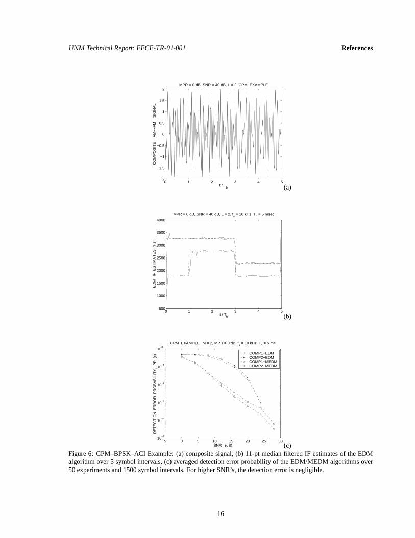
Consider the two–component CPM–ACI example in Fig. (6), where a rectangular pulse shaping functionwith BPSK signaling was used. Themean power ratio(MPR) between the components is 0 dB and the SNRof the signal environment in Fig. (6)(a,b) is 40 dB. The symbol period for the example wasTb = 5 ms at asampling rate of 10 kHz. In this example the EDM algorithm was used to demodulate the two–component CPMsignal. The estimated component IF’s are first 11-pt median filtered and then smoothed using a 3-pt binomialfilter. A conventional BPSK detector is then used for symbol detection for each user. The composite signal forthe example is described in Fig. (6)(a), the IF estimates of the EDM algorithm after 11-pt median filtering andbinomial smoothing are described in Fig. (6)(b), while Fig. 6(c) depicts the average detection error probabilityfor the EDM/MEDM algorithms for various SNR scenarios over 50 experiments and 1500 symbol intervals.

Although the IF estimates are used to make decisions on the bits transmited, it is ultimately the decision errorprobability that we are concerned about in this case. The detection error probability is negligible for SNR valueslarger than 30 dB. Further robustness to noise can be acheived by using the multiband–EDM (MEDM) approachproposed in [28, 27]. Fig. (6)(c) describes the detection error propbabilities of the MEDM approach which areconsiderably better than the corresponding EDM probabilities.

6


Radar Signal Processing Applications

In high frequency radar applications, ocean clutter manifests in the return signal in the form of well definedfrequency shifts from the transmitted radar frequencyfr via [12]

foc = ±√

g frπc

,

where foc corresponds to the Doppler frequency of the ocean clutter signals,fr is the radar carrier frequency andg is the acceleration due to gravity. This effect can be attributed to constructive interference of the scatteringreturn signals. Recent work on modeling ocean clutter has shown that they can be modeled as two narrowbandsignals with time varying frequencies centered about two frequencies corresponding to both first and secondorder scattering [12]. This framework for clutter modeling fits perfectly with the multicomponent AM–FM signalmodel described in the previous section.

It has also been known in the radar community that a target moving with a constant velocity produces aconstant Doppler frequency shift given by

fd =2 frv

c,

wherev is the radial velocity of the target andfr is the radar carrier frequency. Similarly a target that has aconstant radial acceleration will produce linearly changing frequency, i.e., linear–FM or chirp return signals [14].Further work in the target tracking area has focussed on the problem of multiple target tracking, where the returnsignal for each target is modeled as a chirp signal [22].

This is the motivation behind adopting a multicomponent chirp signal model for the multiple target trackingapplication of the form [22]:

x(t) =M

∑k=1

ak cos(wckt +µkt

2) ,

whereωck corresponds to the carrier frequency of thekth target and the IF signal corresponding to thekth targetis a linear–FM signal of the form:

ωk(t) = ωck+2µkt, |t| ≤ T2

,

whereT is the duration of the radar pulse waveform.

Consider the two–component chirp example in Fig. (7). The relevant parameters associated with the com-posite FM signal areFM = 8%, NCS= 0.06, SNR = 40 dB,MPR = 0 dB. With these parameters, there is asignificant amount of spectral overlap between the components. In addition the IF laws of the two componentscross–over. The composite FM signal is described in Fig. (7)(a), the DDF intensity image used for componentperiodicity estimation is shown in Fig. (7)(b). Fig. (7)(c) describes the spectrogram of the composite FM signalwhich shows that there is a significant amount of spectral overlap. Fig. (7)(d) describes the component IF es-timates of the PASED algorithm. The chirp parameters estimated via the PASED algorithm after least-squaresfitting and the actual chirp parameters are tabulated in Fig. (7)(e). The least-squares estimates of the componentIF’s are plotted in Fig. (7)(f).

Further robustness towards noise can be obtained by binomial smoothing of the energy operators used inthe implementation of thediscrete energy separation algorithm(DESA) [32] used in the PASED algorithm.The separated components can be further filtered using a bandpass filter to eliminate noise outside of the signalbandwidth2.

7


Biomedical Signal Processing Applications

The multicomponent AM–FM signal model, specifically a two–component nonlinear transient chirp signal model,has recently been used to model the pulmonary and aortic components of the second heart beat sound [9]. Specif-ically it was shown that both the aortic and the pulmonary components of the second heart beat sound could bemodeled as narrowband chirp signals of short duration, with decreasing IF’s, and with energy distributions con-centrated along their decreasing IF signals. The second heart beat signal can in particular be used as a diagnostictool where it can augment existing methods for detecting paediatric heart disease [38]. The signal separationaspects of the proposal as it relates to the separation of quasiperiodic signals also find application in a relatedbiomedical signal processing problem of materal–foetal ECG signal separation and foetal heart–rate monitoring[33]. Presently used time–frequency tools for analyzing these multicomponent signals suffer from the existanceof cross-terms in the time–frequency representations [9].

Consider the example in Fig. (8) where the algebraic separation (MAS) algorithm was applied to a mixtureof quasi-periodic segments of the ECG data. The ECG signals were obtained from samples of the MIT-BIHpolysomnographic, MGH/MF ECG databases available athttp://ecg.mit.edu/dbsamples.html . The signalfrom the MIT-BIH database has a sampling frequency offs = 340 Hzand the signal from the MGH/MF databasehas a sampling frequency offs = 250Hz. The ECG data used in this example is approximately periodic withperiodsN1 = 12 andN2 = 21 samples which were estimated using the DDF algorithm. The composite signalfor the example is shown in Fig. (8)(a). The DDF intensity image used to estimate the periods is shown inFig. (8)(b). The component estimates (λ = 108) are shown in Fig. (8)(c,d) with RMS component separationerrors are10,13%.

2In this case signal bandwidth refers to twice the Carson bandwidth of the FM signal, i.e., the separation between spectral componentswhose strength is1 %of the carrier strength [1].

8

UNM Technical Report: EECE-TR-01-001 References

References

[1] S. Haykin,Communication Systems, John Wiley& Sons Inc., Second ed., 1983.

[2] G. L. Stuber, “Principles of Mobile Communications,” Kluwer Academic Publishers, Boston, 1996.

[3] J. G. Proakis, “Digital Communications,” Third edition, McGraw Hill Inc., New York 1995.

[4] H. W. Hawkes, ”Study of Adjacent and Co–Channel FM Interference,”Proc. IEE, vol. 138, No. 4, Aug.1991.

[5] Monson H. Hayes, “Statistical Digital Signal Processing and Modeling,” John Wiley& Sons Inc, New York,1996.

[6] L. Cohen, “What is a Multicomponent Signal,”Proc. ICASSP–92, vol. 5, pp. 113 - 116, March 1992.

[7] L. Cohen and C. Lee, ”Instantaneous Frequency, Its standard deviation and Multicomponent Signals,”Proc.of SPIE, Vol. 975, pp. 186-208, 1988.

[8] L. J. Griffiths, “Rapid Measurement of Digital Instantaneous Frequency,IEEE Trans. ASSP, Vol. 23,pp. 207-222, April, 1975.

[9] J. Xu, L.-G. Durand, and P. Pibarot, ”Extraction of the Aortic and Pulmonary Components of the SecondHeart Sound Using a Nonlinear Transient Chirp Signal Model,”IEEE Trans. Biomed. Engg., Vol. 48, No. 3,2001.

[10] B. Friedlander and J. M. Francos, ”Estimation of Amplitude and Phase Parameters of MulticomponentSignals,”IEEE Trans. Sig. Process., vol. 43, pp. 917 - 926, June 1995.

[11] H. B. Lee, ”Eigenvalues and Eigenvectors of Covariance Matrices for Signals Closely Spaced in Frequency,”IEEE Trans. Sig. Process., vol. 40, pp. 2518-2535, Oct. 1992.

[12] M. W. Y. Poon, R. H. Khan, and Son Le–Ngoc, ”A SVD Based Method for Supressing Ocean Clutter inHigh Frequency Radar,”IEEE Trans. Sig. Process., vol. 41, pp. 1421 - 1425, Mar. 1993.

[13] R. Kumaresan, A. G. Sadasiv, and C. S. Ramalingam, and J. F. Kaiser, ”Instantaneous Nonlinear OperatorsFor Tracking Multicomponent Signal Parameters,”Proc. 6th SP Workshop on Statistical Signal and ArrayProcessing, pp. 404 - 407, Oct. 1992.

[14] J. L. Eaves and E. K. Reedy, ”Principles of Modern Radar,” Van Nostrand Reinhold, New York, 1987.

[15] M. Polad and B. Friedlander, “Separation of Co-channel FM/PM signals using the Discrete Polynomial-phase Transform,Proc. IEEE DSP Workshop, pp. 3-6, 1994.

[16] Y. Bar-ness, F. A. Cassara, H. Schachter, and R. Difazio, ”Cross–Coupled Phase–Locked Loop with ClosedLoop Amplitude Control,”IEEE Trans. Commun., vol. 32, pp. 195-198, Feb. 1982.

[17] D. A. Rich, Steven Bo and F. A. Cassara, “Co–Channel FM Interference Suppression Using Adaptive NotchFilters,” IEEE Trans. Commun., Vol. 48, No. 7, pp. 2384-2389, 1994.

[18] B. A. Hedstrom and R. L. Kirlin, ”Co–Channel Signal Separation Using Cross–coupled Digital Phase–Locked Loops,”IEEE Trans. Commun., vol. 44, pp. 1373-1384, Oct. 1996.

[19] A. Potamianos and P. Maragos, ”A Comparison of the Energy Operator and Hilbert Transform Approachesfor Signal and Speech Demodulation,”Signal Processing, vol. 37, pp. 95-120, May 1994.

[20] A. Potamianos and P. Maragos, “Speech Formant Frequency and Bandwidth Tracking Using MultibandEnergy Demodulation,”J. Acoust. Soc. Am., vol. 99, pp. 3795 - 3806, June 1996.

9


[21] A. Potamianos and P. Maragos, “Speech Analysis and Synthesis using an AM-FM Modulation Model,”Speech Communication, Vol. 28, No.3, pp. 195-209, July 1999.

[22] R. M. Liang and K. S. Arun, ”Parameter Estimation For Superimposed Chirp Signals,” inProc. ICASSP–92,pp. 273-276, Mar. 1992.

[23] P. Maragos and A. C. Bovik, “Image Demodulation Using Multidimensional Energy Separation,”J. Opt.Soc. of Am., vol. 12, pp. 1867 - 1876, Sep. 1995.

[24] P. Maragos, J. F. Kaiser, and T. F. Quatieri, “On Amplitude and Frequency Demodulation Using EnergyOperators,”IEEE Trans. Signal Processing, vol. 41, pp. 1532-1550, April 1993.

[25] P. Maragos, J. F. Kaiser, and T. F. Quatieri, ”Energy Separations in Signal Modulations with Application toSpeech Analysis,”IEEE Trans. Signal Processing, vol. 41, pp. 3024 - 3051, Oct. 1993.

[26] A. C. Bovik, P. Maragos, and T. F. Quatieri, ‘ ‘AM–FM Energy Detection and Separation in Noise usingMultiband Energy Operators,”IEEE Trans. Sig. Process., Vol. 41, pp. 3245-3265, Dec. 1993.

[27] B. Santhanam and P. Maragos, “Energy Demodulation of Two–Component AM–FM Signal Mixtures,”IEEESig. Process. Lett., vol. 3, pp. 294-298, Nov. 1996.

[28] B. Santhanam and P. Maragos, “Energy Demodulation of Two-component AM-FM signals with Applicationto Speaker Separation,”Proc. ICASSP-96, vol. 6, pp. 3517 -3520, 1996.

[29] Balasubramaniam Santhanam, “Multicomponent AM–FM Energy Demodulation with Applications to Sig-nal Processing and Communications,”Ph.D Thesis, Georgia Institute of Technology, November 1997.

[30] B. Santhanam and P. Maragos, “Demodulation of Discrete Multicomponent AM–FM Signals Using PeriodicAlgebraic Separation and Demodulation,”Proc. of ICASSP–97, Vol. 3, pp. 2409-2412, 1997.

[31] B. Santhanam and P. Maragos, “Harmonic Analysis and Restoration of Separation Methods for PeriodicSignal Mixtures: Algebraic Separation Vs. Comb Filtering,”Signal Processing, Vol. 69, No. 1, pp. 81-91,1998.

[32] B. Santhanam and P. Maragos, “Multicomponent AM–FM Demodulation via Periodicity–based AlgebraicSeparation and Energy–based Demodulation,”IEEE Trans. Commun., Vol. 48, No. 3, pp. 473-490, 2000.

[33] Balu Santhanam, “Algebraic Separation Applied to Concurrent Vowel Separation and ECG Signal Separa-tion,” Proc. of 34-th Asilomar Conference on Signals, Systems, and Computers, Vol. 2, pp. 1507-1511, Nov.2000.

[34] Balu Santhanam, ”Component Enumeration Of Multicomponent AM–FM signals Via Generalized EnergyOperators,”Submitted towards ICASSP-02, 2001.

[35] W. P. Torres and T. F. Quatieri, “Estimation of modulation based on FM-to-AM transduction: two-sinusoidcase,”IEEE Trans. Sig. Process., Vol. 47, No. 11, pp. 3084-3097, 1999.

[36] C. L. Dimonte and K. S. Arun, ”Tracking the Frequencies of Superimposed Time-varying Harmonics,”Proc.of ICASSP–90, Vol. 2, pp. 2539-2542, 1990.

[37] D. Dimitriadis and P. Maragos, ”An Improved Energy Demodulation Algorithm Using Splines,”Proc.ICASSP-01, Vol. 6, May 2001.

[38] T. S. Leung, P. R. White, J. Cook, W. B. Collins, E. Brown, A. P. Salmon, “Analysis of the second heartsound for diagnosis of paediatric heart disease,”Proc. of IEE, Sci., Measur. and Techn., Vol. 145,pp. 285-290, Nov. 1998.

10


[39] A. Zayezdny and I. Druckmann, ”A New Method of Signal Description and its Applications to SignalProcessing”,Signal Processing, Vol. 22, pp. 153 - 178”, 1991.

[40] P. Gulden, M. Vossiek, E. Storck and P. Heide, ”Application of State Space Frequency Estimation Tech-niques to Radar Systems,”Proc. of ICASSP-01, Vol. 5.

[41] B. D. Rao and K. S. Arun, ”Model Based Processing of Signals: A State Space Approach,”Proc. of IEEE,Vol. 80, No. 2, pp. 283-309, 1992.

[42] M. Wax and T. Kailath, ”Detection of Signals by Information Theoretic Criteria,”IEEE Trans. Acoust.,Speech, Sig. Process, Vol. 33, No. 2, pp. 387-392.

[43] R. B. Dunn, T. F. Quatieri, and J. F. Kaiser, ”Detection of Transient Signals Using the Energy Operator,”Proc. of ICASSP-93, Vol. 3, pp. 145-148.

[44] J. H. L. Hansen, L. Gavidia-Ceballos, J. F. Kaiser, “A nonlinear operator-based speech feature analysismethod with application to vocal fold pathology assessment,”IEEE Trans. Biomed. Engg., Vol. 45, No. 3 ,pp. 300 -313, 1998.

[45] S. Mukhopadhyay and G. C. Ray, “A new interpretation of nonlinear energy operator and its efficacy inspike detection,”IEEE Trans. on Biomed. Engg., Vol. 45, No. 2, pp. 180 -187, 1998.

11


0 200 400 600 800 1000−3

−2

−1

0

1

2

3

TIME SAMPLES

CO

MP

OS

ITE

AM

−−

FM

S

IGN

AL

COMPONENT ENUMERATION EXAMPLE, SNR = 27 dB

(a)

0 200 400 600 800 1000−0.8

−0.6

−0.4

−0.2

0

0.2

0.4

0.6

0.8

1

TIME SAMPLES

COMPONENT ENUMERATION EXAMPLE, SNR = 27 dB

ψ(x

[n])

−

ψ

(x[n

−1

])

(b)

0 200 400 600 800 10000

0.2

0.4

0.6

0.8

1

1.2

1.4

1.6

1.8

2

TIME SAMPLES

ηo = 0.06, SNR = 27 dB

DE

CIS

ION

V

AR

IAB

LE

(c)Figure 2: Component enumeration example: (a) composite AM–FM signal, (b) test signalD[n] after 5-timebinomial smoothing, (c) decision variable for monocomponent detection over the two halves of the signal. Thefirst half of the signal contains two components while the second contains just one component.

12


0 200 400 600 800 1000−3

−2

−1

0

1

2

3

TIME SAMPLE

CO

MP

OS

ITE

A

M−

−F

M S

IGN

AL

SNR = 30 dB, MPR = 6 dB, M = 2, AM = 0 %, CR/IB = 100

(a)

0 200 400 600 800 10001.1

1.2

1.3

1.4

1.5

1.6

1.7

1.8

1.9

TIME SAMPLE

INS

TA

NT

AN

EO

US

A

NG

UL

AR

F

RE

QU

EN

CY

SNR = 30 dB, MPR = 6 dB, M = 2, AM = 0 %, CR/IB = 100

(b)

0 1 2 3 4 50

0.1

0.2

0.3

0.4

0.5

0.6

0.7

0.8

0.9

1

FLOOR((ORD−1)/2)

PR

OP

.

OF

ZE

RO

−D

ET

S

AM

PL

ES

SNR = 30 dB, MPR = 6 dB, M = 2, ηo = 0.1, p

o = 0.8

HALF−2HALF−1

(c)Figure 3: Two–component signal example where both halves of the signal contain 2 components. In the first halfthe component IF’s are well–separated, while in the second half they cross–over.

13


0 200 400 600 800 1000−4

−3

−2

−1

0

1

2

3

4

TIME SAMPLE

CO

MP

OS

ITE

A

M−

−F

M S

IGN

AL

SNR = 30 dB, M = 3, FM = 1%, AM = [2,4,6] %, CR/IB = 100

(a)

0 200 400 600 800 10001.4

1.45

1.5

1.55

1.6

1.65

1.7

1.75

1.8

1.85

TIME SAMPLES

INS

T.

FR

EQ

.

SNR = 30 dB, M = 3, FM = 1%, AM = [2,4,6] %, CR/IB = 100

(b)

0 1 2 3 4 50

0.1

0.2

0.3

0.4

0.5

0.6

0.7

0.8

0.9

1

floor((ORD−1)/2)

PR

OP

. Z

ER

O−

−D

ET

SA

MP

LE

S

SNR = 30 dB, M = 3, po = 0.9, η

o = 0.06

(c)Figure 4: Three–component example: (a) composite AM–FM signal, (b) component IF’s, (c) proportion of zero–determinant samples for various model orders using the Toeplitz-determinant proportion technique with a SNRof 30 dB,ηo = 0.06andpo = 0.9.

14


0 0.5 1 1.5 20

0.1

0.2

0.3

0.4

0.5

0.6

0.7

0.8

0.9

1

NORMALIZED CARRIER SEPARATION (NCS)

PR

OP

. O

F

SA

MP

LE

S

: ψ

(x[n

]) −

ψ(x

[n−

1])

= 0

M = 2, SNR = 30 dB, CR/IB = 100, FM = 1%, AM = [4,8] %

(a)−40 −35 −30 −25 −20 −15 −10 −5 00

0.1

0.2

0.3

0.4

0.5

0.6

0.7

0.8

0.9

1

20log10

(|a2 − a

1| / (a

2 + a

1)) dB

PR

OP

O

F S

AM

PL

ES

: ψ

(x[n

]) −

ψ(x

[n−

1])

M = 2, NCS = 1.5, CR/IB = 100, FM = 1%, AM = 0 %, ηo = 0.38

(b)

10−6

10−4

10−2

100

1

1.1

1.2

1.3

1.4

1.5

1.6

1.7

1.8

1.9

2

po = 0.48 p

o = 0.52

po = 0.55

po = 0.46

PF, PROB. FALSE ALARM

#

OF

C

OM

PO

NE

NT

S

DE

TE

CT

ED

(H

AL

F−

−2

)

CR/IB = 100, MPR = 6 dB, M = 2, AM = 0 %, FM = 1 %

(c)10

−610

−410

−210

02

2.1

2.2

2.3

2.4

2.5

2.6

2.7

2.8

2.9

3

po = 0.6

po = 0.9

po = 0.8p

o = 0.78

po = 0.82

PF, PROB. FALSE ALARM

#

OF

C

OM

PO

NE

NT

S

DE

TE

CT

ED

(H

AL

F−

−1

)

CR/IB = 100, MPR = 6 dB, M = 2, AM = 0 %, FM = 1 %

(d)Figure 5: Effect of NCS and relative component power: (a) proportion of samples whereD[n] = 0 for differentNCS parameters withηo = 0.05, (b) proportion of samples whereD[n] = 0 for different relative componentamplitudes. (c,d) threshold selection: thresholdspo for the two halves in the second two-component example andthe corresponding number of components detected for different false alarm probabilities. The intersection of theset of valid thresholds for both halves is selected for use.

15


0 1 2 3 4 5−2

−1.5

−1

−0.5

0

0.5

1

1.5

2

t / Tb

CO

MP

OS

ITE

A

M−−

FM

S

IGN

AL

MPR = 0 dB, SNR = 40 dB, L = 2, CPM EXAMPLE

(a)

0 1 2 3 4 5500

1000

1500

2000

2500

3000

3500

4000

t / Tb

ED

M

IF E

ST

IMA

TE

S (

Hz)

MPR = 0 dB, SNR = 40 dB, L = 2, fs = 10 kHz, T

b = 5 msec

(b)

−5 0 5 10 15 20 25 3010

−5

10−4

10−3

10−2

10−1

100

SNR (dB)

DE

TE

CT

ION

ER

RO

R P

RO

BA

BIL

ITY

, P

R (

ε)

CPM EXAMPLE, M = 2, MPR = 0 dB, fs = 10 kHz, T

d = 5 ms

COMP1−EDMCOMP2−EDMCOMP1−MEDMCOMP2−MEDM

(c)Figure 6: CPM–BPSK–ACI Example: (a) composite signal, (b) 11-pt median filtered IF estimates of the EDMalgorithm over 5 symbol intervals, (c) averaged detection error probability of the EDM/MEDM algorithms over50 experiments and 1500 symbol intervals. For higher SNR’s, the detection error is negligible.

16


0 150 300 450−2

−1

0

1

2

TIME SAMPLE

CO

MP

OS

ITE

A

M−−

FM

S

IGN

AL

MPR = 0 dB , NCS = 0.06 , FM = 8 % , SNR = 40 dB

(a) LAG PARAMETER 1

LAG

PA

RA

ME

TE

R 2

DDF IMAGE, MPR = 0dB , NCS = 0.06, FM = 8 %, SNR = 40 dB

398 400 402 404 406 408

398

399

400

401

402

403

404

405

406

407

408

(b)

TIME SAMPLE

NO

RM

ALI

ZE

D F

RE

QU

EN

CY

L1 = 400 , L2 = 405 , NCS = 0.06 , FM = 8 %, SNR = 40 dB

0 250 500 750 1000 1250 15000

0.1

0.2

0.3

0.4

0.5

(c)0 100 200 300 400

0.44

0.46

0.48

0.5

0.52

0.54

0.56

TIME SAMPLE

AN

GU

LAR

IF

LE

AS

T−

−S

QU

AR

ES

FIT

, P

AS

ED L1 = 400 , L2 = 405 , NCS = 0.06 , FM = 8 %, SNR = 40 dB

PASED−−IFLS−IF

(d)

k mk mk ck ck ρk

1 0.0006298 0.006305 1.4451 1.4451 0.99382 -0.0006221 -0.006288 1.6771 1.6786 0.9901

(e)Figure 7: Chirp target tracking example: (a) composite FM signal, (b) DDF intensity image associated withcomponent period estimation, (c) spectrogram of the composite FM signal with a FFT size ofN = 1024, aHanning window of lengthL = 75, with R = 2 showing significant spectral overlap, (d) least-squares IF fitversus actual IF, (e) slope and intercept obtained from a least-squares fit of the PASED IF estimates with thecorresponding correlation coefficients.

17


0 20 40 60 80 100−2.5

−2

−1.5

−1

−0.5

0

0.5

1

1.5

2

TIME SAMPLE

CO

MP

OS

ITE

SIG

NA

L

QUASIPERIODIC EXAMPLE: N1 = 12, N

2 = 21

LAG PARAMETER 2

LAG

P

AR

AM

ET

ER

1

DDF INTESNITY IMAGE, N1 = 12, N

2 = 21

10 12 14 16 18 20 22

10

12

14

16

18

20

22

(a) (b)

0 0.05 0.1 0.15−2.5

−2

−1.5

−1

−0.5

0

0.5

1

1.5

TIME in sec

FIR

ST

CO

MP

ON

EN

T

λ = 108 , fs = 250 Hz, N

1 = 12 , N

2 = 21

MAS: λ = 108

ACTUAL

0 0.05 0.1 0.15−1.5

−1

−0.5

0

0.5

1

1.5

TIME in sec

SE

CO

ND

CO

MP

ON

EN

T

λ = 108 , fs = 340 Hz, N

1 = 12 , N

2 = 21

MAS: λ = 108

ACTUAL

(c) (d)Figure 8: Separation of quasi-periodic segments of two ECG signals: (a) the composite signal, (b) periods ofN1 = 12andN2 = 21samples estimated via the DDF algorithm, (c,d) MAS component estimates.

18

non stationary signal analysis, energy demodulation and

Documents