NON-RENEWABLE RESOURCES,EXTRACTION TECHNOLOGY, AND

ENDOGENOUS GROWTH∗

Gregor Schwerhoff† Martin Stuermer ‡

Oct 11, 2018

Abstract

We develop a theory of innovation in non-renewable resource extraction andeconomic growth. Firms increase their economically extractable reserves of non-renewable resources through investment in new extraction technology and reducetheir reserves through extraction. Our model allows us to study the interactionbetween geology and technological change, and its effects on prices, total outputgrowth, and the resource intensity of the economy. The model accommodateslong-term trends in non-renewable resource markets – namely stable prices andexponentially increasing extraction – for which we present data extending backto 1792. The paper suggests that over the long term, increasing consumption ofnon-renewable resources fosters the development of new extraction technologiesand hence offsets the exhaustion of higher quality resource deposits. (JEL codes:O30, O41, Q30)

∗ The views in this paper are those of the author and do not necessarily reflect the views ofthe Federal Reserve Bank of Dallas or the Federal Reserve System. We thank Anton Cheremukhin,Thomas Covert, Klaus Desmet, Maik Heinemann, Martin Hellwig, David Hemous, Charles Jones,Dirk Kruger, Lars Kunze, Florian Neukirchen, Pietro Peretto, Gert Ponitzsch, Salim Rashid, GordonRausser, Paul Romer, Luc Rouge, Sandro Schmidt, Sjak Smulders, Michael Sposi, Jurgen von Hagen,Kei-Mu Yi, and Friedrich-Wilhelm Wellmer for very helpful comments and suggestions. We alsothank participants at the NBER Summer Institute, AEA Annual Meeting, AERE Summer Meeting,EAERE Summer Conference, SURED Conference, AWEEE Workshop, SEEK Conference, USAEEAnnual Meeting, SEA Annual Meeting, University of Chicago, University of Cologne, Universityof Bonn, MPI Bonn, Federal Reserve Bank of Dallas for their comments. We thank Mike Weissfor editing. Emma Marshall, Navi Dhaliwal, Achim Goheer and Ines Gorywoda provided excellentresearch assistance. All errors are our own. An earlier version was published as a Dallas Fed WorkingPaper in 2015 and as a Max Planck Institute for Collective Goods Working Paper in 2012 with thetitle “Non-renewable but inexhaustible: Resources in an endogenous growth model.”†Mercator Research Institute on Global Commons and Climate Change, Email: schwerhoff@mcc-

berlin.net‡Federal Reserve Bank of Dallas, Research Department, Email: martin.stuermer@dal.frb.org.

1 Introduction

This paper contributes to resolving a contradiction between theoretical predictions and

empirical evidence regarding non-renewable resources. According to theory, economic

growth is not limited by non-renewable resources because of three factors: technological

change in the use of resources, substitution of non-renewable resources by capital, and

returns to scale. Given these factors, growth models with a non-renewable resource

typically predict growth in output, decreased non-renewable resource extraction, and

an increase in price (see Groth, 2007; Aghion and Howitt, 1998).

However, it is a well-established fact that these predictions are not in line with

the empirical evidence from the historical evolution of production and prices of non-

renewable resources. The extraction of non-renewable resources has increased over

time, and there is no persistent increase in the real prices of most non-renewable re-

sources over the long run (see Krautkraemer, 1998; Livernois, 2009; Von Hagen, 1989).

To resolve this puzzle, the paper develops a theory of technological change in re-

source extraction in an endogenous growth model. Our starting point is the seminal

paper by Nordhaus (1974), in which he suggests that innovation in extraction tech-

nology helps overcome scarcity by turning mineral deposits in the Earth’s crust into

economically recoverable reserves. Nordhaus also points out that the crustal abun-

dance of non-renewable resources is sufficient to continue consumption for hundreds of

thousands of years if there is technological change.

Modeling technological change in resource extraction in a growth model is challeng-

ing because it adds a layer of dynamic optimization to the model. We boil down the

2

investment and extraction problem to a static problem, which makes our model both

simple enough to solve and rich enough to potentially connect to long-run data.

To our knowledge, our model is the first that allows the study of the interaction be-

tween technological change and geology, and its effects on prices, total output growth,

and its use in the economy. Learning about these effects is important for making pre-

dictions of long-run development of resource prices and for understanding the impact

of resource production on aggregate output. For example, distinguishing between in-

creasing and constant resource prices in the long run is key to the results of a number

of recent papers on climate economics (Acemoglu et al., 2012; Golosov et al., 2014;

Hassler and Sinn, 2012; van der Ploeg and Withagen, 2012).

We add an extractive sector to a standard endogenous growth model of expanding

varieties and directed technological change by Romer (1986) and Acemoglu (2002), such

that aggregate output is produced from a non-renewable resource and an intermediate

good.

Modeling the extractive sector has four components: First, we assume that there is a

continuum of deposits of declining grades. The quantity of the non-renewable resource

is distributed such that it increases exponentially as the ore grades of deposits decrease,

as a local approximation to Ahrens (1953, 1954) fundamental law of geochemistry.

Although we recognize that non-renewable resources are ultimately finite in supply,

we make the assumption that the underlying resource quantity goes to infinity for all

practical economic purposes as the grade of the deposits approaches zero. Without

innovation in extraction technology, the extraction cost is assumed to be infinitely

high.

3

Second, we build on Nordhaus (1974) idea that reserves are akin to working capital

or inventory of economically extractable resources. Firms can invest in grade specific

extraction technology to subsequently convert deposits of lower grades into economi-

cally extractable reserves. We assume that R&D investment exhibits decreasing returns

in making deposits of lower grades extractable, as historical evidence suggests. Once

converted into a reserve, the firm that developed the technology can extract the re-

source at a fixed operational cost.

Third, new technology diffuses to all other firms. As each new technology is specific

to a deposit of a certain grade, it cannot be used to extract resources from deposits of

lower grades. However, all firms can build on existing technology when they invest in

developing new technology for deposits of lower grades. The idea is that firms can, for

example, use the shovel invented by another firm but have a cost to train employees to

use it for a specific deposit of lower grade. As technology diffuses, firms only maximize

current profits in their R&D investment decisions in equilibrium.

Finally, the non-renewable resource is a homogeneous good. Despite a fully com-

petitive resource market in the long run, firms invest in extractive technology because

it is grade specific. Most similar to this understanding of innovation is Desmet and

Rossi-Hansberg (2014). We abstract from other possible features like uncertainty about

deposits, negative externalities from resource extraction, recycling, and short-run price

fluctuations.

Our model accommodates historical trends in the prices and production of major

non-renewable resources, as well as world real GDP for which we present data extend-

ing back to 1792. It implies a constant resource price equal to marginal cost over

4

the long run. Extraction firms face constant R&D costs in converting one unit of the

resource into a new reserve. This is due to the offsetting interaction between techno-

logical change and geology: (i) new extraction technology exhibits decreasing returns

in making deposits of lower grades extractable; (ii) the resource quantity is geologically

distributed such that it increases exponentially as the grade of its deposits decreases.

The resource price depends negatively on the average crustal concentration of the

resource. For example, our model predicts that iron ore prices are on average lower

than copper prices, because iron is more abundant (5 percent of crustal mass) than

copper (0.007 percent). The price is also negatively affected by the average effect of

technology in terms of making lower grade deposits extractable. For example, the

average effect might be larger for deposits that can be extracted in open pit mines (e.g.

coal) than for deposits requiring underground operations (e.g. crude oil). This implies

that coal prices are lower than crude oil price in the long term.

The resource intensity of the economy, defined as the resource quantity used to

produce one unit of aggregate output, is positively affected by the average geologi-

cal abundance and the average effect of extraction technology, while the elasticity of

substitution has a strong negative effect. If the resource and the intermediate good

are complements, the resource intensity of the economy is relatively high, while it is

significantly lower in the case of the two being substitutes. As the resource intensity is

constant in equilibrium, firms extract the non-renewable resource at the same rate as

aggregate output.

Aggregate output growth is constant on the balanced growth path. Our model

predicts that a higher abundance of a particular resource or a higher average effect of

5

extractive technology in terms of lower grades positively impact aggregate growth in

the long run.

The extractive sector features only constant returns to scale. In contrast to the

intermediate good sector, where firms can make use of the entire stock of technology

for production, firms in the extractive sector can only use the flow of new technology

to convert deposits of lower grades into new reserves. Earlier developed technologies

are grade specific and the related deposits are exhausted. The stock of extraction tech-

nology therefore grows proportionally to output, while technology in the intermediate

good sectors increases at the same rate as aggregate output.

The paper contributes to a literature that mostly builds on the seminal Hotelling

(1931) optimal depletion model. Heal (1976) introduces a non-renewable resource,

which is inexhaustible, but extractable at different grades and costs. Extraction costs

increase with cumulative extraction, but then remain constant when a “backstop tech-

nology” (Heal, 1976, p. 371) is reached. Slade (1982) adds exogenous technological

change in extraction technology to the Hotelling (1931) model and predicts a U-shaped

relative price curve. Cynthia-Lin and Wagner (2007) use a similar model with an in-

exhaustible non-renewable resource and exogenous technological change. They obtain

a constant relative price with increasing extraction.

There are three papers, to our knowledge, that like ours include technological

change in the extraction of a non-renewable resource in an endogenous growth model.

Fourgeaud et al. (1982) focuses on explaining sudden fluctuations in the development

of non-renewable resource prices by allowing the resource stock to grow in a stepwise

manner through technological change. Tahvonen and Salo (2001) model the transition

6

from a non-renewable energy resource to a renewable energy resource. Their model

follows a learning-by-doing approach as technological change is linearly related to the

level of extraction and the level of productive capital. It explains decreasing prices and

the increasing use of a non-renewable energy resource over a particular time period

before prices increase in the long term. Hart (2016) models resource extraction and

demand in a growth model with exogenous technological change. After a temporary

“frontier phase” with a constant resource price and consumption rising at a rate only

close to aggregate output, the economy needs to extract resources from greater depths.

Subsequently, a long-run balanced growth path is reached with constant resource con-

sumption and prices that rise in line with wages.

In Section 2, we document stylized facts on the long-term development of non-

renewable resource prices, production, and world real GDP. We also provide evidence

for the major assumptions of our model regarding geology and technological change.

Section 3 introduces the main mechanisms of the theory with regard to technological

change and geology. Section 4 describes the microeconomic foundations of the extrac-

tive sector and its innovation process. Section 5 presents the growth model, and section

6 derives and discusses theoretical predictions. In Section 8 we draw conclusions.

2 Prices, Resource Production, and Aggregate Out-

put over the Long Term

We collect annual data for major non-renewable resource markets going back to 1792.

Statistical tests indicate that real non-renewable resource prices are roughly trend-less

7

and that worldwide primary production as well as world real GDP grow roughly at a

constant rate.

Figure 1 presents data on the real prices of five major base metals and crude oil.

Real prices exhibit strong short-term fluctuations. We test the null hypothesis that the

growth rates of the real prices are not significantly different from zero. As the regression

results in Table 2 in the appendix show, this null hypothesis cannot be rejected. The

real prices are trend-less. This is in line with evidence over other time periods provided

by Krautkraemer (1998), Von Hagen (1989), Cynthia-Lin and Wagner (2007), Stuermer

(2016). The real price for crude oil exhibits structural breaks over the long term, as

shown in Dvir and Rogoff (2010). Overall, the literature is certainly not conclusive (see

Pindyck, 1999; Lee et al., 2006; Slade, 1982; Jacks, 2013; Harvey et al., 2010), but we

believe the evidence is sufficient to take trend-less prices as a motivation for our model.

Figure 2 shows that the world primary production of the examined non-renewable

resources and world real GDP approximately exhibit constant positive growth rates

since 1792. A closer statistical examination confirms that the production of non-

renewable resources exhibits significantly positive growth rates in the long term (see

table 3 in the appendix).

8

Note

s:A

llp

rice

s,ex

cep

tfo

rth

ep

rice

of

cru

de

oil,

are

pri

ces

of

the

Lond

on

Met

al

Exch

an

ge

an

dit

spre

dec

esso

rs.

As

the

pri

ceof

the

Lon

don

Met

al

Exch

ange

use

dto

be

den

om

inate

din

Ste

rlin

gin

earl

ier

tim

es,

we

have

conver

ted

thes

ep

rice

sto

U.S

.-D

ollar

by

usi

ng

his

tori

cal

exch

ange

rate

sfr

om

Offi

cer

(2011).

We

use

the

U.S

.-C

on

sum

erP

rice

Ind

expro

vid

edby

Offi

cer

an

dW

illiam

son

(2011)

an

dth

eU

.S.

Bu

reau

of

Lab

or

Sta

tist

ics

(2010)

for

defl

ati

ng

pri

ces

wit

hth

eb

ase

yea

r1980-8

2.

Th

ese

con

dary

y-a

xis

rela

tes

toth

ep

rice

of

cru

de

oil.

For

data

sou

rces

an

ddes

crip

tion

see

Stu

erm

er(2

013).

Fig

ure

1:R

eal

pri

ces

ofm

ajo

rm

iner

alco

mm

odit

ies

innat

ura

llo

gs.

9

For

data

sou

rces

and

des

crip

tion

see

Stu

erm

er(2

013).

Fig

ure

2:W

orld

pri

mar

ypro

duct

ion

ofnon

-ren

ewab

lere

sourc

esan

dw

orld

real

GD

Pin

logs

.

10

Crude oil production follows this pattern up to 1975. Inclusion of the time period

from 1975 until 2009 reveals a statistically significant negative trend and, therefore,

declining growth rates over time due to a structural break in the oil market (Dvir

and Rogoff, 2010; Hamilton, 2009). In the case of primary aluminum production, we

also find declining growth rates over time and hence, no exponential growth of the

production level. This might be attributable to the increasing importance of recycling

(see data by U.S. Geological Survey, 2011a).

Overall, we take these stylized facts as motivation to build a model that exhibits

trend-less resource prices and constant growth in the worldwide production of non-

renewable resources and in world aggregate output.

3 Non-Renewable Resources and Extraction Tech-

nology

Technological change in the extractive sector is different from other sectors due to its

interaction with geology. As higher grade geological deposits get depleted under exist-

ing technology, firms develop new technology to convert lower grade deposits to become

extractable and to ultimately continue resource production. We call this “Factor Ex-

tracting Technological Change”. As the resource is a function of improving extraction

technology and geology, it is like working capital. This is in contrast to factor aug-

menting technological change, which makes the use of a fixed factor more efficient.

In the following we introduce key concepts of our theory by describing stylized facts

on the geological environment and technological change in the extractive sector and

11

how we model them. We then lay out their interaction and introduce the concept of a

non-renewable but inexhaustible resource.

3.1 Geological Environment

The earth’s crust contains deposits of non-renewable resources, such as copper or crude

oil. Table 1 shows that the crustal abundance of several major non-renewable resources

is large, orders of magnitude greater than existing reserves (see also Nordhaus (1974);

Aguilera et al. (2012); Rogner (1997)).

Reserves are defined as the fraction of the total resource quantity in the Earth’s

crust that can be economically extracted with current technology (see U.S. Geological

Survey (2011c)).

Reserves/ Crustal abundance/Annual production Annual production

(Years) (Years)

Aluminum 1391a 48,800,000,000bc

Copper 43a 95,000,000ab

Iron 78a 1,350,000,000ab

Lead 21a 70.000.000ab

Tin 17a 144.000ab

Zinc 21a 187.500.000ab

Gold 20d 27,160,000ef

Coal2 129g 1,400,0006iCrude oil3 55g

Natural Gas4 59g

Notes: Definition of Reserves: “Identified resources that meet specified minimum physical and chemical criteria relatedto current mining and production practices and that can be economically extracted or produced at the time of determina-tion.”(Source: Schulz et al., 2017) Definition of Crustal Abundance: Total quantity of a resource in the earth crust. 1datafor bauxite, 2includes lignite and hard coal, 3includes conventional and unconventional oil, 4includes conventional andunconventional gas, 5all organic carbon in the earth’s crust. Sources: aU.S. Geological Survey (2012b), bPerman et al.(2003), cU.S. Geological Survey (2011c),dU.S. Geological Survey (2011b),eNordhaus (1974),fU.S. Geological Survey(2010), gFederal Institute for Geosciences and Natural Resources (2011) giLittke and Welte (1992).

Table 1: Availability of selected non-renewable resources in years of production left inthe reserve and crustal mass based on current annual mine production.1

12

Non-renewable resources are not uniformly concentrated in the earth’s crust. Rather,

some deposits are highly concentrated with a specific resource, and other deposits are

less so. In our model, we define the grade O of a deposit as the average concentration

of the resource; the grade ranges from 0 to 100 percent. The grade distinguishes the

difficulty of extraction, where a low grade is very difficult. There are also other char-

acteristics of mineral deposits like depth and thickness. We focus on the grade, as this

is the most important characteristic.

3.2 Extraction Technology

Technology development in the extractive sector is special, because it is making lower

grade deposits economically extractable that, due to high costs, have not been previ-

ously extractable. Technological change increases reserves (see Simpson, 1999; Nord-

haus, 1974, and others). This implies that technology is grades-specific. Firms need

to adjust their technology or make new inventions in order to extract resources from

deposits of lower grades.

Empirical evidence suggests that the marginal effect of extraction technology on

grades declines (see Lasserre and Ouellette, 1991; Mudd, 2007; Simpson, 1999; Wellmer,

2008). For example, Radetzki (2009) and Bartos (2002) describe how technological

changes in mining equipment, prospecting, and metallurgy have gradually made pos-

sible the extraction of copper from lower grade deposits. The average ore grades of

copper mines, for example, have decreased from about twenty percent 5,000 years ago

to currently below one percent (Radetzki, 2009). Figure 3 illustrates this development

using the example of U.S. copper mines. Gerst (2008) and Mudd (2007) come to similar

13

results for worldwide copper mines and the mining of different base-metals in Australia.

Figure 3: The historical development of mining of various grades of copper in the U.S.Source: Scholz and Wellmer (2012)

We observe similar developments for hydrocarbons. Using the example of the off-

shore oil industry, Managi et al. (2004) show that technological change has offset the

cost-increasing degradation of resources. Crude oil has been extracted from ever deeper

sources in the Gulf of Mexico, as Figure 10 in the appendix shows. Furthermore, tech-

nological change and high prices have made it profitable to extract hydrocarbons from

unconventional sources, such as tight oil, oil sands, and liquid natural gas (International

Energy Agency, 2012).

Figures 3 (and 10 in the appendix) also show that decreases in grades have slowed

as technological development progressed. Under the reasonable assumption that global

R&D investment has stayed constant or increased in real terms, there are decreasing

14

returns to R&D in terms of making mining from deposits of lower grades economically

feasible.

The extraction technology function maps the state of the extraction technology N

onto the extractable grade O? of the deposits (see figure 4). The extractable grade is

a decreasing convex function of technology. Technological development makes deposits

economically extractable, but there are decreasing returns in terms of grades:

O?(NR) = e−µNR , µ ∈ R+ NR ∈ (0,∞) . (1)

The grade O? is the lowest grade that firms can extract with technology level NR.

Technological change, NR, expands the range of grades that can be extracted. Hence,

as technology develops, the extractable ore grade falls. The curve in Figure 4 starts

with deposits of close to a 100 percent ore grade, which represents the state of the world

several thousand years ago. We assume that extractable ore grades only get closer to

zero in the long term.

15

100%

(N,O?)

(N ′, O?′)

Level of technological progress NR

Dep

osit

sS

ort

edby

Extr

act

ab

leO

reG

rad

eO∗

Figure 4: Extraction Technology Function.

The curvature parameter of the extraction technology function is µ. If, for example,

µ is high, the average effect of new technology on converting deposits to reserves in

terms of grades is relatively high.

3.3 Geological Function

Resources are not evenly distributed across deposits in the earth’s crust. Ahrens (1953,

1954) states in the fundamental law of geochemistry that each resource exhibits a log-

normal grade-quantity distribution in the earth’s crust, postulating a decided positive

skewness.2 Hence, the resource content of deposits increases as its grades decrease. The

2Geologists do not fully agree on a log-normal distribution, especially regarding very low concen-trations of metals, which might be mined in the distant future. Skinner (1979) and Gordon et al.(2007) propose a discontinuity in the distribution due to the so-called “mineralogical barrier,” the ap-proximate point below which metal atoms are trapped by atomic substitution. Gerst (2008) concludesin his geological study of copper deposits that he can neither confirm nor refute these two hypothe-ses. However, based on worldwide data on copper deposits over the past 200 years, he finds evidencefor a log-normal relationship between copper production and ore grades. Mudd (2007) analyzes thehistorical evolution of extraction and grades of deposits for different base metals in Australia. Hefinds that production has increased at a constant rate, while grades have consistently declined. We

16

reason is that as grades decrease deposits become larger. See figure 5 for geological

evidence on copper.

Figure 5: Cumulative grade-quantity distribution of copper in the Earth’s crust.Source: Gerst (2008).

We define Q(O?) as the “cumulative resource quantity”, that is the quantity of the

resource that is (or has been - as it might have been extracted already) available in

deposits of grades in the interval [O?, 1). The lower bound is the lowest grade O? that

firms can extract with technology level NR. These resources are either part of firms’

reserves or have been used in past production. The geological function takes the form:

Q(O?) = −δ ln(O?), δ ∈ R+ O? ∈ (0, 1) . (2)

Figure 6 plots the function. The figure is read in direction of the red arrow. Tech-

recognize that there remains uncertainty about the geological distribution, specially regarding hydro-carbons with their distinct formation processes. However, we believe that it is reasonable to assumethat a non-renewable resource is distributed according to a log-normal relationship between the gradeof deposits and quantity.

17

100%

(O?′, Q′)

(O?, Q)

Deposits Sorted by Extractable Ore Grade O∗

Cum

ula

tive

Quanti

tyQ

(O∗ )

Figure 6: Geological Function.

nology development shifts the extractable deposits from grade O? down to grade O?′.

The respective cumulative resource quantity increases from Q to Q′.

The functional form implies that the cumulative quantity of the resource approaches

infinity as the grade of deposits gets closer to zero. Although we recognize that non-

renewable resources are ultimately finite in supply, we assume that the underlying

resource quantity goes to infinity for any time frame that is relevant for human eco-

nomic activity. This assumption is analogue to households maximizing over an infinite

horizon.

Parameter δ controls the curvature of the function. If δ is high, the marginal effect

on the quantity of the non-resources from shifting to deposits of lower grades is high.

It implies that the average concentration of the non-renewable resource is high in the

crustal mass.

18

3.4 A Non-Renewable but Inexhaustible Resource

Technological change in resource extraction offsets the depletion of economically ex-

tractable reserves of non-renewable resources (Simpson, 1999, and others). Hence,

reserves are drawn down by extraction, but increase by technological change in extrac-

tion technology.

The extraction of non-renewable resources from lower grade deposits goes hand in

hand with increases of reserves over time. Figure 7 shows that copper reserves have

increased by more than 700 percent since 1950. Crude oil reserves have doubled since

the 1980s (see figure 11 in the appendix).3

Figure 7: Historical evolution of world copper reserves from 1950 to 2016. Sources:Tilton and Lagos C.C. (2007), USGS.

3Note that world copper production increased by a roughly equivalent percentage since 1950, whileworld oil production increased by roughly 30 percent since 1980.

19

We propose to call a non-renewable resource, which features reserves that are drawn

down by extraction, but increase by technological progress in extraction technology,

a new renewable but inexhaustible resource. The traditional way of modeling non-

renewable resource follows Hotelling (1931). Resource extraction R equals the draw-

down of the resource stock S:

R = −S with St ≥ 0, Rt ≥ 0 and S0 > 0.

Major assumptions of this approach are a fixed know resource stock and no extraction

cost or innovation.

In contrast, extraction of the non-renewable but inexhaustible resource Rt equals

the change in the reserves S and new reserves due to technological development Qt.

Reserves S are defined as non-renewable resource in the ground that can be extracted

with current technology.

Rt = −St + Qt, St ≥ 0, Qt ≥ 0, Rt ≥ 0. (3)

New reserves due to technological change Qt are a function of the extractable ore

grade O?, which is a function of grades-specific extraction technology NR:

Qt = F (O?(NR)). (4)

Note that in our model R is the stock of resources that has ever been extracted. In

the case of metals, these resources might either still be in use in the so called “techno-

20

sphere” (partly due to recycling), in inventories, or have ended up on landfills. In the

case of fossil fuels, R is the stock of resources that are either still in inventories, in

transportation to a combustion unit, or have been burnt. S is the stock of resources in

firms’ reserves. Q is the stock of resources that have ever been converted to reserves.

Hence, R + S = Q. We call Q the cumulative resource quantity.

3.5 Marginal Effect of Extraction Technology on Reserves

The technology function, equation (1), and the geology function, equation (2), have

offsetting effects. This leads to a constant marginal effect of new technology on new

reserves.

Proposition 1 The cumulative resource quantity develops proportionally to the level

of extraction technology NR:

Q(O?(NRt)) = δµNRt .

The marginal effect of new extraction technology on the cumulative resource quantity

Qt equals:

dQ(O?(NRt))

dNR

= δµ .

As the natural exponential in (1) and the natural log in equation (2) cancel out, the

relationship between investment in technology and the cumulative resource quantity is

linear.

21

Proof of Proposition 1

Q(O?(NRt)) = −δ ln(O?(NRt))

= −δ ln(e−µNRt)

= µδNRt

2

The intuition is that two offsetting effects cause this result: (i) the cumulative

resource quantity is geologically distributed such that it implies increasing returns in

terms of new reserves as the grade of deposits decline; (ii) new extraction technology

exhibits decreasing returns in terms of making lower grade deposits extractable.

Figure 8 illustrates how the interaction of the geological and the extraction technol-

ogy functions leads to a linear relationship between technology and reserves. The upper

left panel shows how two equal steps in advancing technology from 0 to N and from

N to N ′, lead to diminishing returns in terms of extractable ore grades O? and O?′,

where O?′ − O? ≺ O?. The lower right panel depicts how the two related extractable

ore grades O? and O?′ map into equally sized steps in the cumulative resource quantity

Q and Q′, where Q′ −Q = Q. Finally, the lower left panel summarizes the linear rela-

tionship between the level technological progress and the cumulative resource quantity

as a result of the two functions.

22

Figure 8: The interaction between the extraction technology function (upper left panel)and the extraction technology function (lower right panel) leads to a linear relationshipbetween technology NR and cumulative resource quantity Q (lower right panel).

23

The equations in Proposition 1 depend on the shapes of the geological function and

the technology function. If the respective parameters δ and µ are high, the marginal

return on new extraction technology will also be high.

The constant effect of technology on new reserves implies that the social value

of an innovation is equal to the private value. R&D development does not cause an

exhaustion of the resource. Future innovations are not reduced in profitability. No

positive or negative spill-overs occur in our model.

4 The Extractive Sector

We first set up a simple extractive sector. There are two different types of firms,

extraction firms and technology firms. The former buy technology from the technology

firms and extract the resource, while the latter innovate and produce technology. The

sector is constructed in analogy to Acemoglu (2002) to ease comparison. We use

continuous time to facilitate interpretation of the necessary conditions and the analysis

of equilibrium dynamics.

4.1 Extractive Firms

We consider a large number of infinitely small extractive firms.4 As we model long-run

trends in the extractive sector, we assume that the sector is fully competitive and firms

take the demand for the non-renewable resource as given.5 Firms fully know about the

4We assume that the firm level production functions exhibit constant returns to scale, so there isno loss of generality in focusing on aggregate production functions.

5Historically, producer efforts to raise prices were successful in some non-oil commodity markets,though short-lived as longer-run price elasticities proved to be high (see Radetzki, 2008; Herfindahl,1959; Rausser and Stuermer, 2016). Similarly, a number of academic studies discard OPEC’s ability to

24

distribution of the resource across deposits.

Firms use new technology to extract the resource from their reserves S. Reserves

are defined as non-renewable resource in underground deposits that can be extracted

with the grades-specific technology at a constant extraction cost φ > 0. We assume

that the marginal extraction cost for deposits not classified as reserves are infinitely

high, φ =∞. Technology depreciates fully after use.

Firms can expand their reserves by investing in new grades-specific technology of

variety j. Each new technology j makes deposits of lower grades O extractable. We

assume decreasing returns of technological change in terms of ore grades (see equation

(1)). Extraction firms can purchase the new technology from sector-specific technology

firms at price χR. This allows firms to claim ownership of all of the non-renewable

resource in the respective additional deposits. Firms declare these deposits their new

reserves.

Combining equations (3) and Proposition 1, the net rate of change of firms’ reserves

is:

St = −Rt + Qt St ≥ 0, Qt ≥ 0, Rt ≥ 0,

where new reserves equal:6

Qt = δµNR. (5)

Extractive firms’ profit function is: πER = pRR− φR− χRδµN ,

raise prices over the long term (see Aguilera and Radetzki, 2016, for an overview). This is in line withhistorical evidence that OPEC has never constrained members’ capacity expansions, which would bea precondition for long-lasting price interventions (Aguilera and Radetzki, 2016)

6Please see Appendix 1.1 for the derivation of this equation.

25

4.2 Technology Firms in the Extractive Sector

New extraction technologies are supplied by sector-specific technology firms. The in-

novation possibilities frontier, which determines how new technologies are created, is

assumed to take the following form:7

NR = ηRMR . (6)

Technology firms can spend one unit of the final good for R&D investment M at time

t to generate a flow rate ηR > 0 of new patents, respectively. Each technology firm can

hence freely enter the market if it develops a patent for a new extraction technology

(or machine) j at this cost.8 Firms enter the market until the value of entering, namely

profits, equals market entry cost. The free entry condition is thus

1

ηR= πRt .

The new technology is non-rival, but excludable because it applies only to specific

deposits. Technology diffuses immediately. Once a firm has invented a technology, each

technology can be produced at a fixed marginal cost ψR > 0. Each technology is only

produced once, as the respective deposits are depleted and new technologies need to

be invented.

Even though technology firms have a monopoly on patent j, different machines can

7We assume in line with Acemoglu (2002) that there is no aggregate uncertainty in the innovationprocess. There is idiosyncratic uncertainty, but with many different technology firms undertakingresearch, equation 6 holds deterministically at the aggregate level.

8We use j to denominate both, new machines and technology firms, because each firm can onlyinvent one new machine in line with Acemoglu (2002).

26

be regarded as substitutes since they all give access to additional deposits of the same

homogenous resource. As a result, technology firms in the extractive sector do not have

market power. Machine prices χR(j) result from the market equilibrium of demand and

marginal cost. Patents have still value, because extraction firms have to buy machines

of varieties j to extent their reserves and ultimately to continue producing.

In the extractive sector, the value of a technology firm that discovers a new machine

depends hence only on instantaneous profit.

VR(j) = πR(j) = χR(j)− ψR , (7)

This allows us to boil down a dynamic optimization problem to a static one. It

makes the model solvable and computable. At the same time, the model is rich enough

to derive meaningful theoretical predictions about the relationship between technolog-

ical change, geology and economic growth.

Figure 9: Timing and Firms’ Problem

Start period t:

Extracting firms

observe resource

demand R and

demand new

machines N

Early period t:

Technology

firms enter the

market, develop

and sell new

machines N

Mid period t:

Extracting

firms convert

deposits

into reserves

Late period t:

Extracting

firms extract

R and sell it

to aggregate

producer

Figure 9 illustrates the timing in our model. At the start of period t, extraction firms

observe the resource demand from the aggregate production sector and they demand

new technologies from the technology firms. In the early period of t, technology firms

observe this demand and decide if they want to invest into developing new machines

27

and enter the market. Each firm produces one machine based on the patent that it

develops and sells it to the extraction firms. In the later period of t, extraction firms

convert deposits to reserves based on the new machines and extract the resource.

5 Extraction Technology in an Endogenous Growth

Model

We embed the extractive sector in an endogenous growth model with two sectors, and

take the framework by Romer (1986) and Acemoglu (2002) as a starting point. The

general equilibrium model setup and the intermediate goods sector will be presented

in this section.

5.1 Setup

We consider a standard setup of an economy with a representative consumer that has

constant relative risk aversion preferences:

∫ ∞0

C1−θt − 1

1− θe−ρtdt .

The variable Ct denotes consumption of aggregate output at time t, ρ is the discount

rate, and θ is the coefficient of relative risk aversion.

The aggregate production function combines two inputs, namely an intermediate

good Z and a non-renewable resource R, with a constant elasticity of substitution:

28

Y =[γZ

ε−1ε + (1− γ)R

ε−1ε

] εε−1

. (8)

The distribution parameter γ ∈ (0, 1) indicates their respective importance in pro-

ducing aggregate output Y . The elasticity of substitution is ε > 0, when the resource

is not essential for aggregate production (see Dasgupta and Heal, 1980).

The budget constraint of the representative consumer is: C+I+M ≤ Y . Aggregate

spending on machines is denoted by I and aggregate R&D investment by M , where

M = MZ +MR. The usual no-Ponzi game conditions apply.

Setting the price of the final good as the numeraire gives:

[γεp1−ε

Z + (1− γ)εp1−εR

] 11−ε = 1 , (9)

where pZ is the price index of the intermediate good and pR is the price index of the

non-renewable resource. Intertemporal prices of the intermediate good are given by

the interest rate [rt]∞T=0.

5.2 Intermediate Good Sector

The intermediate good sector follows the basic setup of Acemoglu (2002). It consists

of a large number of infinitely small firms that produce the intermediate good, and

technology firms that produce sector-specific technologies.9

9Like in the extractive sector, we assume that the firm level production functions exhibit constantreturns to scale, so there is no loss of generality in focusing on aggregate production functions. Firmsin the extractive and in the intermediate sectors use different types of machines to produce the non-renewable resource and the intermediate good, respectively. Firms are owned by the representative

29

Firms produce an intermediate good Z according to the production function:

Z =1

1− βZ

(∫ Nz

0

xz(j)1−βZdj

)LβZ , (10)

where xZ(j) refers to the number of machines used for each machine variety j in

the production of the intermediate good, L is labor, which is in fixed supply, and βZ

is ∈ (0, 1). This implies that machines in the intermediate good sector are partial

complements.10

All intermediate good machines are supplied by sector-specific technology firms that

each have one fully enforced perpetual patent on the respective machine variety. As

machines are partial complements, technology firms have some degree of market power

and can set the price for machines. The price charged by these firms at time t is

denoted χZ(j) for j ∈ [0, NZ(t)]. Once invented, machines can be produced at a fixed

marginal cost ψZ > 0.

The innovation possibilities frontier is assumed to take a similar form like in the

extractive sector: NZ = ηRMZ . Technology firms can spend one unit of the final good

for R&D investment MZ at time t to generate flow rate ηZ > 0 of new patents. Each

firm hence needs 1ηZ

units of final output to develop a new machine variety. Technology

firms can freely enter the market if they develop a patent for a new machine variety.

They can only invent one new variety.

household.10While machines of type j in the intermediate sector can be used infinitely often, a machine of

variety j in the resource sector is grade-specific and essential to extracting the resource from depositsof certain grades O. A machine of variety j in the extractive sector is therefore only used once, andthe range of machines employed to produce resources at time t is NR. In contrast, the intermediategood sector can use the full range of machines [0, NZ(t)] complementing labor.

30

6 Characterization of Equilibrium

We define the allocation in this economy by the following objects: time paths of con-

sumption levels, aggregate spending on machines, and aggregate R&D expenditure,

[Ct, It,Mt]∞t=0; time paths of available machine varieties, [NRt, NZt, ]

∞t=0; time paths of

prices and quantities of each machine, [χRt(j), xRt(j)]∞j∈[0,NRt]t

and [χZt(j), xZt(j)]∞j∈[0,NZt],t

;

the present discounted value of profits VR and VZ , and time paths of interest rates and

wages, [rt, wt]∞t=0.

An equilibrium is an allocation in which all technology firms in the intermediate

good sector choose [χZt(j), xZt(j)]∞j∈[0,NZ(t)],t to maximize profits. Machine prices in

the extractive sector χRt(j) result from the market equilibrium, because extraction

technology firms are in full competition and only produce one machine per patent.

The evolution of [NRt, NZt]∞t=0 is determined by free entry; the time paths of factor

prices, [r, w]∞t=0, are consistent with market clearing; and the time paths of [Ct, It,Mt]∞t=0

are consistent with household maximization.

6.1 The Final Good Producer

The final good producer demands the intermediate good and the resource for aggre-

gate production. Prices and quantities for both are determined in a fully competitive

equilibrium. Taking the first order condition with respect to the intermediate good and

31

the non-renewable resource in (8), we obtain the demand for the intermediate good

Z =Y (1− γ)ε

pεZ,

and the demand for the resource

R =Y (1− γ)ε

pεR. (11)

6.2 Extraction Firms

To characterize the (unique) equilibrium, we first determine the demand for machine

varieties in the extractive sector.11 Machine prices and the number of machine varieties

are determined in a market equilibrium between extractive firms and technology firms.

Firms optimization problem is static since machines depreciate fully after use.

In equilibrium, it is profit maximizing for firms to not keep reserves, S(j) = 0.12 It

follows that the production function of extractive firms is

Rt = δµNRt. (12)

Extractive firms face a cost for producing Rt units of resource given by Ω(Rt) =

RtχR1δµ

, where χR is the machine price charged by the extraction technology firms.

The marginal cost is Ω′(Rt) = χR1δµ

. The inverse supply function of the resource is

11Please see Appendix 1.2 for the respective derivations regarding intermediate good firms.12If we assumed stochastic technological change, extractive firms would keep a positive stock of

reserves St to insure against a series of bad draws in R&D. Reserves would grow over time in line withaggregate growth. The result would, however, remain the same: In the long term, resource extractionequals new reserves.

32

hence constant and we obtain a market equilibrium at

pR = χR1

δµ

and

Rt =Y (1− γ)ε

(χR1δµ

)ε. (13)

Using (12), we obtain the demand for machines:

NR =1

δµ

Y (1− γ)ε

(χR1δµ

)ε. (14)

6.3 Technology Firms in the Extractive Sector

In the extractive sector, the demand function for extraction technologies (14) is isoe-

lastic, but there is perfect competition between the different suppliers of extraction

technologies, as machine varieties are perfect substitutes.13 Because only one machine

is produced for each machine variety j, the constant rental rate χR that all monopolists

j ∈ [Nt−h, Nt] limh→0 charge includes the cost of machine production ψR and a mark-up

that refinances R&D costs. The rental rate is the result of a competitive market and

derived from (13). It equals:

χR(j) =(Y/R

) 1ε

(1− γ)δµ. (15)

To complete the description of equilibrium on the technology side, we impose the

13Please see Appendix 1.3 for the respective derivations for technology firms in the intermediategood sector.

33

free-entry condition, (4.2). Like in the intermediate sector, markups are used to cover

technology expenditure in the extractive sector. Combining equations (7) and (15),

we obtain that the net present discounted value of profits of technology firms from

developing one new machine variety is:

VR(j) = πR(j) = χR(j)− ψR =(Y/R

) 1ε

(1− γ)δµ− ψR . (16)

To compute the equilibrium quantity of machines and machine prices in the extractive

sector, we first rearrange (16) with respect to R and consider the free entry condition.

We obtain

Rt =Y (1− γ)ε((1ηR

+ ψR

)1δµ

)ε . (17)

We insert (17) into (15) and obtain the equilibrium machine price.

χR(j) =1

ηR+ ψR . (18)

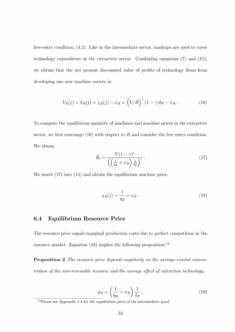
6.4 Equilibrium Resource Price

The resource price equals marginal production costs due to perfect competition in the

resource market. Equation (18) implies the following proposition:14

Proposition 2 The resource price depends negatively on the average crustal concen-

tration of the non-renewable resource and the average effect of extraction technology:

pR =

(1

ηR+ ψR

)1

δµ, (19)

14Please see Appendix 1.4 for the equilibrium price of the intermediate good.

34

where ψR reflects the marginal cost of producing the machine and ηR is a markup that

serves to compensate technology firms for R&D cost.

The intuition is as follows: If, for example, δ is high, the average crustal concen-

tration of the resource is high (see equation (2)) and the price is low. If µ is high, the

average effect of new extraction technology on converting deposits of lower grades to

reserves is high (see equation (1)). This implies a lower resource price. The resource

price level also depends negatively on the cost parameter of R&D development ηR.

6.5 Resource Intensity of the Economy

Substituting equation (19) into the resource demand equation (11), we obtain the ratio

of resource consumption to aggregate output.

Proposition 3 The resource intensity of the economy is positively affected by the aver-

age crustal concentration of the resource and the average effect of extraction technology:

R

Y= (1− γ)ε

[(

1

ηR+ ψR)

1

δµ

]−ε.

The resource intensity of the economy is negatively affected by the elasticity of substi-

tution if (1− γ)ε[( 1ηR

+ ψR) 1δµ

]−ε< 1 and positively otherwise.

6.6 The Growth Rate on the Balanced Growth Path

We define the BGP equilibrium as an equilibrium path where consumption grows at

the constant rate g∗ and the relative price p is constant. From (9) this definition implies

35

that pZt and pRt are also constant.

Proposition 4 There exists a unique BGP equilibrium in which the relative technolo-

gies are given by equation (32) in the appendix, and consumption and output grow at

the rate15

g = θ−1

βηZL[γ−ε − (1− γγ

)ε(1

ηRδµ+ψRδµ

)1−ε] 1

1−ε1β

− ρ

. (20)

The growth rate of the economy is positively influenced by (i) the crustal concen-

tration of the non-renewable resource δ and (ii) the effect of R&D investment in terms

of lower ore grades µ.

Adding the extractive sector to the standard model by Acemoglu (2002), changes

the interest part of the Euler equation, g = θ−1(r − ρ).16 Instead of two exogenous

production factors, the interest rate r in our model only includes labor, but adds the

resource price, as pZ depends on pR according to equation (30).

If (1−γ)ε(ηRδµ)1−ε < 1 holds, then the substitution between the intermediate good

and the resource is low and R&D investment in extraction technology have a small yield

in terms of additional reserves. The effect that economic growth is impossible if the

resource cannot be substituted by other production factors is known as the “limits to

growth” effect in the literature (see Dasgupta and Heal, 1979, p. 196 for example).

When the effect occurs, growth is limited in models with a positive initial stock of

15Starting with any NR(0) > 0 and NZ(0) > 0, there exists a unique equilibrium path. IfNR(0)/NZ(0) < (NR/NZ)∗ as given by (32), then MRt > 0 and MZt = 0 until NRt/NZt = (NR/NZ)∗.If NR(0)/NZ(0) > (NR/NZ)∗, then MRt = 0 and MZt > 0 until NRt/NZt = (NR/NZ)∗. It can also beverified that there are simple transitional dynamics in this economy whereby starting with technologylevels NR(0) and NZ(0), there always exists a unique equilibrium path, and it involves the economymonotonically converging to the BGP equilibrium of (20) like in Acemoglu (2002).

16There is no capital in this model, but agents delay consumption by investing in R&D as a functionof the interest rate.

36

resources, because the initial resource stock can only be consumed in this case. In our

model, growth is impossible, because there is no initial stock and the economy is not

productive enough to generate the necessary technology. When the inequality does not

hold, the economy is on a balanced growth path.

6.7 Technology Growth

We derive the growth rates of technology in the two sectors from equations (12), (11),

and (19). The stock of technology in the intermediate good sector grows at the same

rate as the economy.

Proposition 5 The stock of extraction technology grows proportionally to output ac-

cording to:

NR = (1− γ)εY (1/ηR + ψR)−ε (δµ)ε−1 .

In contrast to the intermediate good sector, where firms can make use of the stock of

technology, firms in the extractive sector can only use the flow of new technology to

convert deposits of lower grades into new reserves. Previously developed technology

cannot be employed because it is grade specific, and deposits of that particular grade

have already been depleted. Note also that firms in the extractive sector need to

invest a larger share of total output to attain the same rate of growth in technology in

comparison to firms in the intermediate good sector.

The effects of the two parameters δ from the geological function and µ from the

extraction technology function on NR depend on the elasticity of substitution ε. Like

in Acemoglu (2002), there are two opposing effects at play: the first is a price effect.

37

Technology investments are directed towards the sector of the scarce good. The second

is a market size effect, meaning that technology investments are directed to the larger

sector.

If the goods of the two sectors are complements (ε < 1), the price effect dominates.

An increase in δ or µ lowers the cost of resource production and the resource price, but

the technology growth rate in the resource sector decelerates, because R&D investment

is directed towards the complementary intermediate good sector. If the resource and

the intermediate good are substitutes (ε > 1), the market size effect dominates. An

increase in δ or µ makes resources cheaper and causes an acceleration in the technology

growth rate in the resource sector, because more of the lower cost resource is demanded.

7 The Case of Multiple Resources

We now extend the model and replace the generic resource with a set of distinct re-

sources. We do so in analogy to a generic capital stock as in many growth models.

We define resources RMult, resource prices pMultR and resource investments MMult

R as

38

aggregates of the respective variables of different resources i ∈ [0, G],

RMult =

(∑i

Rσ−1σ

i

) σσ−1

,

pMultR =

(∑i

Ri

Rpσ−1σ

Ri

) 11−σ

,

MMultR =

∑i

MRi ,

R

Y= (1− γ)εpMult

R

−ε,

g = θ−1

(βηZL

[γ−ε −

(1− γγ

)εpMultR

1−ε] 1

1−ε1β

− ρ

),

where σ is the elasticity of substitution between the different resources. Note that

the aggregate resource price consists of the average of the individual resources weighted

by their share in physical production.

This extension can be used to make theoretical predictions. As an example, we

focus here on the relative price of two resources, aluminum a and copper c. Using

equation (19) and assuming that the cost of producing machines ψR and the flow rate

of innovations ηR are uniform across resources,we obtain that prices depend solely on

geological and technological parameters:

pcR = (δcµc)−1 and paR = (δaµa)−1.

Total resource production equals

R =(Rcσ−1

σ + Raσ−1σ

) σσ−1

,

39

From this, we derive the following theoretical predictions:

pcRpaR

= (δaµa)(δcµc)

and Rc

Ra= ( (δcµc)

(δaµa))σ,

pcRRc

paRRa = ( δ

aµa

δcµc)σ−1 and

NcR

NaR

= ( δcµc

(δaµa))σ−1(

ηcRηaR

)σ

We can investigate what happens when a new resource gets used (e.g. aluminum

was not used until the end of the XIX th). If we assume that σ > 1 and that the

resource is immediately at its steady-state price, the price of the resource aggregate will

immediately decline and the growth rate of the economy will increase: pR = ((δc1δc2)σ−1+

(δa1δa2)σ−1)

11−σ .

Alternatively, a progressive increase in aluminum technology, NaR = ηaR min (Na

R/N, 1)

MaR, would generate an initial decline in the real price (as ηaR min (Na

R/N, 1) increases)

and faster growth in the use of aluminum initially. This is in line with historical evi-

dence from the copper and aluminum markets.

7.1 Discussion

We discuss the assumptions made in section 5, the comparison to other models with

non-renewable resources, and the ultimate finiteness of the resource.

We chose the functional forms of the geological function and the extraction tech-

nology based on empirical evidence. Our model provides theoretical results that are

consistent with the historical evolution resource prices and production. However, for

making long-term predictions based on our model, a natural question is wow other

functional forms of the two functions would affect the predictions of the model. First,

if any of the two function is discontinuous with an unanticipated break, at which the

40

respective parameters changes to either δ′ ∈ R+ or µ′ ∈ R+, there will be two balanced

growth paths: one for the period before, and one for the period after the break. Both

paths would behave according to the model’s predictions. As an illustration, assume

that δ′ > δ. According to proposition (1), the amount of resources in reserved obtained

per unit of investment into extraction technology would increase. This would lower the

resource price in proposition (2), increase the resource intensity in proposition (3), and

increase the growth rate of the economy (see proposition (26)).

Second, if one or both of them has a different form, the effects on resource price,

resource intensity of the economy, and growth rate will depend on the resulting changes

for proposition 1. Intuitively, if the increasing returns in the geology function do not

offset the decreasing returns in the technology function, the resource price will increase

over time, the resource intensity will decline and the growth rate of the economy will

decline as well. There will still be no scarcity rent like in Hotelling (1931)17, because

firms continue to extract resources in a competitive market and firms cannot take prices

above marginal cost.

If the increasing returns in the geology function more than offset the decreasing

returns in the technology function, the resource price will decline and the resource

becomes more abundant. As a result, the resource price will decline, the resource

intensity increase, and the growth rate of the economy will go up. Our model can

also be generalized to this case, since the condition that resource prices equal marginal

resource extraction cost would extend to this case. Prices cannot be below marginal

extraction cost, since firms would make negative profits. Different forms of the function

17Note that a scarcity rent has not yet been found empirically (see e.g. Hart and Spiro, 2011)

41

could also lead to a mixture of these two cases. For example, the resource price increases

for some time and then declines. This would cause a declining and then increasing

resource intensity and growth rate of the economy.

How does our model compare to other models with non-renewable resources? We

make the convenient assumption that the quantity of non-renewable resources is for all

practical economic purposes approaches infinite. As a consequence, resource availability

does not limit growth if there is investment in technological change. Substitution of

capital for non-renewable resources, technological change in the use of the resource,

and increasing returns to scale are therefore not necessary for sustained growth as in

Groth (2007) or Aghion and Howitt (1998). If the resource was finite in our model, the

extractive sector would behave in the same way as in standard models with a sector

based on Hotelling (1931). As Dasgupta and Heal (1980) point out, in this case the

growth rate of the economy depends strongly on the degree of substitution between the

resource and other economic inputs. For ε > 1, the resource is non-essential; for ε < 1,

the total output that the economy is capable of producing is finite. The production

function is, therefore, only interesting for the Cobb-Douglas case.

Our model suggests that the non-renewable resource can be thought of as a form of

capital: if the extractive firms invest in R&D in extraction technology, the resource is

extractable without limits as an input to aggregate production. This feature marks a

distinctive difference from models such as the one of Bretschger and Smulders (2012).

They investigate the effect of various assumptions about substitutability and a decen-

tralized market on long-run growth, but keep the assumption of a finite non-renewable

resource. Without this assumption, the elasticity of substitution between the non-

42

renewable resource and other input factors is no longer central to the analysis of limits

to growth.

Some might argue that the relationship described in proposition 1 cannot continue

to hold in the future as the amount of non-renewable resources in the earth’s crust is

ultimately finite. Scarcity will become increasingly important, and the scarcity rent

will be positive even in the present. However, for understanding current prices and

consumption patterns, current expectations about future developments are important.

Given that the quantities of available resources indicated in table 1 are very large, their

ultimate end far in the future should approximately not affect economic behavior today

and in the near future. The relationship described in proposition 1 seems to have held

in the past and looks likely to hold for the foreseeable future. Since in the long term,

extracted resources equal the resources added to reserves due to R&D in extraction

technology, the price for a unit of the resource will equal the extraction cost plus the

per-unit cost of R&D and hence, stay constant in the long term. This may explain why

scarcity rents cannot be found empirically.

8 Conclusion

This paper examines interaction between geology and technology and its impact on

the resource price, total output growth, and the resource intensity of the economy. We

argue that economic growth causes the production and use of a non-renewable resource

to increase at a constant rate. The marginal production cost of non-renewable resources

stay constant in the long term. Economic growth enables firms to invest in extraction

43

technology R&D, which makes resources from deposits of lower grades economically

extractable. We help explain the long-term evolution of non-renewable resource prices

and world production for more than 200 years. If historical trends in technological

progress continue, it is possible that non-renewable resources are, within a time frame

relevant for humanity, practically inexhaustible.

Our model makes simplifying but reasonable assumptions, which render our model

analytically solvable. However, we believe that a less simple model would essentially

provide the same results. There are four major simplifications in our model, which

should be examined in more detail in future extensions. First, there is no uncertainty

in R&D development, and therefore no incentive for firms to keep a positive amount

of the non-renewable resource in their reserves. If R&D development is stochastic as

in Dasgupta and Stiglitz (1981), there would be a need for firms to keep reserves.

Second, our model features perfect competition in the extractive sector. We could

obtain a model with monopolistic competition in the extractive sector by introducing

explicitly privately-owned deposits. A firm would need to pay a certain upfront cost

or exploration cost in order to acquire a mineral deposit. This upfront cost would give

technology firms a certain monopoly power as they develop machines that are specific

to a single deposit.

Third, extractive firms could face a trade-off between accepting high extraction

costs due to a lower technology level and investing in R&D to reduce extraction costs.

A more general extraction technology function would provide the basis to generalize

this assumption.

Fourth, our model does not include recycling. Recycling has become more important

44

for metal production over time due to the increasing abundance of recyclable materials

and the comparatively low energy requirements (see Wellmer and Dalheimer, 2012).

Introducing recycling into our model would further strengthen the argument of this

paper, as it increases the economically extractable stock of the non-renewable resource.

Finally, firms’ holdings of reserves are zero in our model owing to the constant price

and no uncertainty about research outcomes. We leave it to future work to lift the

assumption of no aggregate uncertainty and to model positive reserve holdings, as we

observe than empirically.

45

9 Authors’ affiliations

Martin Stuermer is with the Research Department of the Federal Reserve Bank of Dal-

las.

Gregor Schwerhoff is currently with the Deutsche Gesellschaft fur Internationale Zusam-

menarbeit (GIZ) GmbH and will be with the World Bank starting November 2018.

46

References

Acemoglu, D. (2002). Directed technical change. The Review of Economic Studies,

69(4):781–809.

Acemoglu, D., Aghion, P., Bursztyn, L., and Hemous, D. (2012). The environment and

directed technical change. American Economic Review, 102(1):131–66.

Aghion, P. and Howitt, P. (1998). Endogenous growth theory. MIT Press, London.

Aguilera, R., Eggert, R., Lagos C.C., G., and Tilton, J. (2012). Is depletion likely

to create significant scarcities of future petroleum resources? In Sinding-Larsen,

R. and Wellmer, F., editors, Non-renewable resource issues, pages 45–82. Springer

Netherlands, Dordrecht.

Aguilera, R. and Radetzki, M. (2016). The Price of Oil. Cambridge University Press.

Ahrens, L. (1953). A fundamental law of geochemistry. Nature, 172:1148.

Ahrens, L. (1954). The lognormal distribution of the elements (a fundamental law of

geochemistry and its subsidiary). Geochimica et Cosmochimica Acta, 5(2):49–73.

Bartos, P. (2002). SX-EW copper and the technology cycle. Resources Policy, 28(3-

4):85–94.

Bretschger, L. and Smulders, S. (2012). Sustainability and substitution of exhaustible

natural resources: How structural change affects long-term R&D investments. Jour-

nal of Economic Dynamics and Control, 36(4):536 – 549.

British Petroleum (2013). BP statistical review of world energy. http://www.bp.com/

(accessed on March 14, 2014).

Cynthia-Lin, C. and Wagner, G. (2007). Steady-state growth in a Hotelling model of re-

source extraction. Journal of Environmental Economics and Management, 54(1):68–

83.

Dasgupta, P. and Heal, G. (1979). Economic theory and exhaustible resources. Cam-

bridge Economic Handbooks (EUA).

Dasgupta, P. and Heal, G. (1980). Economic theory and exhaustible resources. Cam-

bridge University Press, Cambridge, U.K.

Dasgupta, P. and Stiglitz, J. (1981). Resource depletion under technological uncer-

tainty. Econometrica, 49(1):85–104.

47

Desmet, K. and Rossi-Hansberg, E. (2014). Innovation in space. American Economic

Review, 102(3):447–452.

Dvir, E. and Rogoff, K. (2010). The three epochs of oil. mimeo.

Federal Institute for Geosciences and Natural Resources (2011). Reserven, Resourcen,

Verfugbarkeit von Energierohstoffen 2011. Federal Institute for Geosciences and Nat-

ural Resources, Hanover, Germany.

Fourgeaud, C., Lenclud, B., and Michel, P. (1982). Technological renewal of natural

resource stocks. Journal of Economic Dynamics and Control, 4(1):1–36.

Gerst, M. (2008). Revisiting the cumulative grade-tonnage relationship for major cop-

per ore types. Economic Geology, 103(3):615.

Golosov, M., Hassler, J., Krusell, P., and Tsyvinski, A. (2014). Optimal taxes on fossil

fuel in general equilibrium. Econometrica, 82(1):41–88.

Gordon, R., Bertram, M., and Graedel, T. (2007). On the sustainability of metal

supplies: a response to Tilton and Lagos. Resources Policy, 32(1-2):24–28.

Groth, C. (2007). A new growth perspective on non-renewable resources. In Bretschger,

L. and Smulders, S., editors, Sustainable Resource Use and Economic Dynamics,

chapter 7, pages 127–163. Springer Netherlands, Dordrecht.

Hamilton, J. (2009). Understanding crude oil prices. The Energy Journal, 30(2):179–

206.

Hart (2016). Non-renewable resources in the long run. Journal of Economic Dynamics

and Control, 71:1–20.

Hart, R. and Spiro, D. (2011). The elephant in Hotelling’s room. Energy Policy,

39(12):7834–7838.

Harvey, D. I., Kellard, N. M., Madsen, J. B., and Wohar, M. E. (2010). The Prebisch-

Singer hypothesis: four centuries of evidence. The Review of Economics and Statis-

tics, 92(2):367–377.

Hassler, J. and Sinn, H.-W. (2012). The fossil episode. Technical report, CESifo

Working Paper: Energy and Climate Economics.

Heal, G. (1976). The relationship between price and extraction cost for a resource with

a backstop technology. The Bell Journal of Economics, 7(2):371–378.

48

Herfindahl, O. (1959). Copper costs and prices: 1870-1957. Published for Resources

for the Future by Johns Hopkins Press, Baltimore.

Hotelling, H. (1931). The economics of exhaustible resources. Journal of Political

Economy, 39(2):137–175.

International Energy Agency (2012). World energy outlook 2012. International Energy

Agency, Paris.

Jacks, D. S. (2013). From boom to bust: A typology of real commodity prices in the

long run. Technical report, National Bureau of Economic Research.

Krautkraemer, J. (1998). Nonrenewable resource scarcity. Journal of Economic Liter-

ature, 36(4):2065–2107.

Lasserre, P. and Ouellette, P. (1991). The measurement of productivity and scarcity

rents: the case of asbestos in canada. Journal of Econometrics, 48(3):287–312.

Lee, J., List, J., and Strazicich, M. (2006). Non-renewable resource prices: determin-

istic or stochastic trends? Journal of Environmental Economics and Management,

51(3):354–370.

Littke, R. and Welte, D. (1992). Hydrocarbon source rocks. Cambridge University

Press, Cambridge, U.K.

Livernois, J. (2009). On the empirical significance of the Hotelling rule. Review of

Environmental Economics and Policy, 3(1):22–41.

Managi, S., Opaluch, J., Jin, D., and Grigalunas, T. (2004). Technological change

and depletion in offshore oil and gas. Journal of Environmental Economics and

Management, 47(2):388–409.

Mudd, G. (2007). An analysis of historic production trends in australian base metal

mining. Ore Geology Reviews, 32(1):227–261.

Nordhaus, W. (1974). Resources as a constraint on growth. American Economic

Review, 64(2):22–26.

Officer, L. (2011). Dollar-Pound exchange rate from 1791. MeasuringWorth.

Officer, L. and Williamson, S. (2011). The annual consumer price index for the united

states, 1774-2010. http://www.measuringworth.com/uscpi/ (accessed November 2,

2011).

49

Perman, R., Yue, M., McGilvray, J., and Common, M. (2003). Natural resource and

environmental economics. Pearson Education, Edinburgh.

Pindyck, R. (1999). The long-run evolution of energy prices. The Energy Journal,

20(2):1–28.

Radetzki, M. (2008). A handbook of primary commodities in the global economy. Cam-

bridge Univ. Press, Cambridge, U.K.

Radetzki, M. (2009). Seven thousand years in the service of humanity: the history of

copper, the red metal. Resources Policy, 34(4):176–184.

Rausser, G. and Stuermer, M. (2016). Collusion in the copper commodity market: A

long-run perspectivel. Manuscripty.

Rogner, H. (1997). An assessment of world hydrocarbon resources. Annual Review of

Energy and the Environment, 22(1):217–262.

Romer, P. M. (1986). Increasing returns and long-run growth. Journal of political

economy, 94(5):1002–1037.

Scholz, R. and Wellmer, F. (2012). Approaching a dynamic view on the availability

of mineral resources: what we may learn from the case of phosphorus? Global

Environmental Change, 23(1):11–27.

Schulz, K. J., DeYoung Jr., J. H., Bradley, D. C., and Seal II, R. R. (2017). Critical

Mineral Resources of the United States. An Introduction, volume U.S. Geological

Survey Professional Paper 1802. U.S. Department of the Interior.

Simpson, R., editor (1999). Productivity in natural resource industries: improvement

through innovation. RFF Press, Washington, D.C.

Skinner, B. (1979). A second iron age ahead? Studies in Environmental Science,

3:559–575.

Slade, M. (1982). Trends in natural-resource commodity prices: an analysis of the time

domain. Journal of Environmental Economics and Management, 9(2):122–137.

Stuermer, M. (2013). What drives mineral commodity markets in the long run?

PhD thesis, University of Bonn. http://hss.ulb.uni-bonn.de/2013/3313/3313.pdf (ac-

cessed September 4, 2013).

Stuermer, M. (2016). 150 years of boom and bust: What drives mineral commodity

prices? Macroeconomic Dynamics, forthcoming.

50

Tahvonen, O. and Salo, S. (2001). Economic growth and transitions between renewable

and nonrenewable energy resources. European Economic Review, 45(8):1379–1398.

Tilton, J. and Lagos C.C., G. (2007). Assessing the long-run availability of copper.

Resources Policy, 32(1-2):19–23.

U.S. Bureau of Labor Statistics (2010). Consumer price index. All urban consumers.

U.S. city average. All items.

U.S. Bureau of Mines (1991). Minerals yearbook. 1991. Metals and minerals. U.S.

Bureau of Mines, Washington, D.C.

U.S. Geological Survey (2010). Gold statistics. U.S. Geological Survey, Reston, V.A.

U.S. Geological Survey (2011a). Historical statistics for mineral and material com-

modities in the United States. U.S. Geological Survey, Reston, V.A.

U.S. Geological Survey (2011b). Mineral commodity summaries 2011. U.S. Geological

Survey, Reston, V.A.

U.S. Geological Survey (2011c). Minerals yearbook 2010. U.S. Geological Survey,

Reston, V.A.

U.S. Geological Survey (2012a). Historical statistics for mineral and material com-

modities in the United States. U.S. Geological Survey, Reston, V.A.

U.S. Geological Survey (2012b). Mineral commodity summaries 2012. U.S. Geological

Survey, Reston, V. A.

van der Ploeg, F. and Withagen, C. (2012). Too much coal, too little oil. Journal of

Public Economics, 96(1):62–77.

Von Hagen, J. (1989). Relative commodity prices and cointegration. Journal of Busi-

ness & Economic Statistics, 7(4):497–503.

Wellmer, F. (2008). Reserves and resources of the geosphere, terms so often misun-

derstood. Is the life index of reserves of natural resources a guide to the future.

Zeitschrift der Deutschen Gesellschaft fur Geowissenschaften, 159(4):575–590.

Wellmer, F. and Dalheimer, M. (2012). The feedback control cycle as regulator of past

and future mineral supply. Mineralium Deposita, 47:713–729.

51

Appendix 1

Appendix 1.1 Derivation of Extraction Firms’ New Reserves

Equation (5) is derived in the following way: Firms can buy machines j to increase

their reserves by:

Qt = δµ limh→0

1

h

∫ NR(t)

NR(t−h)

xR(j)(1−β)dj , (21)

where xR(j) refers to the number of machines used for each machine variety j.

We assume that β = 0 in the extractive sector, because firms invest into technol-

ogy to continue resource production. If firms do not invest, extraction cost becomes

infinitely high. Firms are indifferent from which deposits they extract the resource. A

machine of variety j in the resource sector is grade-specific and essential to extracting

the resource from deposits of certain grades. A machine of variety j in the extractive

sector is therefore only used once, and the range of machines employed to produce

resources at time t is NR. In contrast, the intermediate good sector can use machine

types infinitely often and hence the full range of machines [0, NZ(t)] complementing

labor. Under the assumption that xR(j) = 1, equation (21) turns into:

Qt = δµ limh→0

1

h

∫ NR(t)

NR(t−h)

1dj

= δµNR .

52

Appendix 1.2 Solving for the Equilibrium: Intermediate Good

Firms

For the intermediate good firms, the maximization problem can be written as

maxL,xZ(j)j∈[0,NZt]

pZZ − wL−∫ NZ

0

χZ(j)xZ(j)dj .

The problem is static, as machines depreciate fully.

The FOC with respect to xZ(j) immediately implies the following isoelastic demand

function for machines:

xZt(j) =

(pZt

χZt(j)

)1/β

L , (22)

for all j ∈ [0, NZ(t)] and all t,

Appendix 1.3 Solving for the Equilibrium: Technology Firms

in the Intermediate Good Sector

Substituting (22) into (23), we calculate the FOC with respect to machine prices in

the intermediate good sector: χZ(j):(

pZχZ(j)

) 1βL − (χZ(j) − ψR)p

1β

Z1βχZ(j)

1β−1L = 0.

Hence, the solution of the maximization problem of any monopolist j ∈ [0, NZ ] involves

setting the same price in every period according to

53

χZt(j) =ψR

1− βfor all j and t .

The value of a technology firm in the intermediate good sector that discovers one

of the machines is given by the standard formula for the present discounted value of

profits:

VZ(j) =

∫ ∞t

exp

(−∫ s

t

r(s′)ds′)πZ(j)ds .

Instantaneous profits are denoted

πZ(j) = (χZ(j)− ψZ)xZ(j) , (23)

where r is the market interest rate, and xZ(j) and χZ(j) are the profit-maximizing

choices for the technology monopolist in the intermediate good sector.

All monopolists in the intermediate good sector charge a constant rental rate equal

to a markup over their marginal cost of machine production, ψR. We normalize the

marginal cost of machine production to ψR ≡ (1− β) (remember that the elasticity of

substitution between machines is ε ≡ 1β), so that

χZt(j) = χZ = 1 for all j and t . (24)

In the intermediate good sector, substituting the machine prices (24) into the de-

mand function (22) yields: xZt(j) = p1/βZt L for all j and all t.

54

Since the machine quantities do not depend on the identity of the machine, only on

the sector that is being served, profits are also independent of machine variety in both

sectors. Firms are symmetric.

In particular profits of technology firms in the intermediate good sector are πZt =

βp1/βZt L. This implies that the net present discounted value of monopolists only depends

on the sector and can be denoted by VZt.

Combining the demand for machines (22) with the production function of the in-

termediate good sector (10) yields the derived production function:

Z(t) =1

1− βp

1−ββ

Zt NZtL, (25)

The equivalent equation in the extractive sector is (12), because there is no op-

timization over the number of machines by the extraction technology firms, as the

demand for machines per machine variety is one.

Appendix 1.4 Equilibrium Prices

Prices of the intermediate good and the non-renewable resource are derived from the

marginal product conditions of the final good technology, (8), which imply

p ≡ pRpZ

=1− γγ

(R

Z

)− 1ε

=1− γγ

δµNR

11−βp

1−ββ

L NZL

− 1ε

55

There is no derived elasticity of substitution in analogy to Acemoglu (2002), be-

cause there is only one fixed factor, namely L in the intermediate good sector. In

the extractive sector, resources are produced by machines from deposits. The first

line of this expression simply defines p as the relative price between the intermediate

good and the non-renewable resource, and uses the fact that the ratio of the marginal

productivities of the two goods must be equal to this relative price. The second line

substitutes from (25) and (12). There are no relative factor prices in this economy like

in Acemoglu (2002), because there is only one fixed factor in the economy, namely L

in the intermediate good sector.

Appendix 1.5 Proof for the Balanced Growth Path

We define the BGP equilibrium as an equilibrium path where consumption grows at

the constant rate g∗ and the relative price p is constant. From (9) this definition implies

that pZt and pRt are also constant.

Household optimization implies

CtCt

=1

θ(rt − ρ),

and

limt→∞

[exp

(−∫ t

0

r(s)ds

)(NZtVZt + NRtVRt)

]= 0,

which uses the fact that NZtVZt + NRtVRt is the total value of corporate assets in the

economy. In the resource sector, only new machine varieties produce profit.

56

The consumer earns wages from working in the intermediate good sector and earns

interest on investing in technology MZ . The budget constraint thus is C = wL+ rMZ .

Maximizing utility in equation (5.1) with respect to consumption and investments

yields the first order conditions C−θe−ρt = λ and λ = −rλ so that the growth rate of

consumption is

gc = θ−1(r − ρ) . (26)

This is equal to output growth on the balanced growth path. We can thus solve for

the interest rate and obtain r = θg + ρ. The free entry condition for the technology

firms imposes that profits from investing in patents must be zero. Revenue per unit of

R&D investment is given by VZ , cost is equal to 1ηZ

. Consequently, we obtain ηZVZ = 1.

Making use of equation (27), we obtainηZβp

1βZ L

r= 1. Solving this for r and substituting

it into equation (26) we obtain the following proposition:

g = θ−1(βηZLp1β

Z − ρ) .

Adding the extractive sector to the standard model by Acemoglu (2002), changes

the interest part of the Euler equation, g = θ−1(r − ρ).18 Instead of two exogenous

production factors, the interest rate r in our model only includes labor, but adds the

resource price, as pZ depends on pR according to equation (30). Together with (19),

this yields the growth rate on the balanced growth path.

Proposition 6 Suppose that

18There is no capital in this model, but agents delay consumption by investing in R&D as a functionof the interest rate.

57

β[(1− γ)εR(ηRR)σ−1 + γεZ(ηZL)σ−1

] 1σ−1

> ρ, and

(1− θ)β[γεR(ηRR)σ−1 + γεZ(ηZL)σ−1

] 1σ−1

< ρ.

If (1 − γ)ε(ηRδµ)1−ε < 1 the economy cannot produce. Otherwise, there exists a

unique BGP equilibrium in which the relative technologies are given by equation (32),

and consumption and output grow at the rate in equation (20).19

19Starting with any NR(0) > 0 and NZ(0) > 0, there exists a unique equilibrium path. IfNR(0)/NZ(0) < (NR/NZ)∗ as given by (32), then MRt > 0 and MZt = 0 until NRt/NZt = (NR/NZ)∗.If NR(0)/NZ(0) > (NR/NZ)∗, then MRt = 0 and MZt > 0 until NRt/NZt = (NR/NZ)∗. It can also beverified that there are simple transitional dynamics in this economy whereby starting with technologylevels NR(0) and NZ(0), there always exists a unique equilibrium path, and it involves the economymonotonically converging to the BGP equilibrium of (20) like in Acemoglu (2002).

58

Appendix 2 Directed Technological Change

Let VZ and VR be the BGP net present discounted values of new innovations in the two

sectors. Then the Hamilton-Jacobi-Bellman Equation version of the value function for

the intermediate good sector rtVZ(j) − VZ(j) = πZ(j) and the free entry condition of

extraction technology firms imply that

VZ =βp

1/βZ L

r∗, and VR = χR(j)− ψR , (27)

where r∗ is the BGP interest rate, while pZ is the BGP price of the intermediate good

and χR(j) is the BGP machine price in the extractive sector.

The greater is VR relative to relative to VZ , the greater are the incentives to develop

machines in the extractive sector rather than developing machines in the intermediate

good sector. Taking the ratio of the two equations in (27) and including the equilibrium

machine price (18) yields

VRVZ

=χR(j)− ψR

1rβp

1β

ZL=

1ηR

1rβp

1β

ZL. (28)

This expression highlights the effects on the direction of technological change

1. The price effect manifests itself because VR/VZ is decreasing in pZ . The greater

is the intermediate good price, the smaller is VR/VZ and thus the greater are the

incentives to invent technology complementing labor. Since goods produced by

59

the relatively scarce factor are relatively more expensive, the price effect favors

technologies complementing the scarce factor. The resource price pR does not

affect VR/VZ due to perfect competition among extraction technology firms and

a flat supply curve.

2. The market size effect is a consequence of the fact that VR/VZ is decreasing in

L. Consequently an increase in the supply of labor translates into a greater

market for the technology complementing labor. The market size effect in the

intermediate good sector is defined by the exogenous factor labor. There is no

equivalent in the extractive sector.

3. Finally, the cost of developing one new machine variety in terms of final output

also influences the direction of technological change. If the parameter η increases,

the cost goes down, the relative profitability VR/VZ decreases, and therefore the

incentive to invent extraction technology declines.

Since the intermediate good price is endogenous, combining (26) with (28) the relative

profitability of the technologies becomes

VRVZ

=

1ηR

1rβ

pR γ1−γ

(δµNR

11−β p

1−ββ

Z NZL

) 1ε

1β

L

(29)

Rearranging equation (9) we obtain

pZ =

(γ−ε −

(1− γγ

)εp1−εR

) 11−ε

. (30)

60

Combining (30) and (19), we can eliminate relative prices, and the relative profitability

of technologies becomes:

VRVZ

=

1ηR

1rβ

((γ−ε −

(1−γγ

)ε ((1ηR

+ ψR

)1µδ

)1−ε) 1

1−ε) 1

β

L

.

Using the free-entry conditions and assuming that both of them hold as equalities, we

obtain the following BGP technology market clearing condition:

ηZVZ = ηRVR. (31)

Combining 31 with 29, we obtain the following BGP ratio of relative technologies and

solving for NRNZ

yields:

(NR

NZ

)∗=

((r

ηZβL

)β1− γγpR

)εLp

1−ββ

Z

(1− β)δµ

where the asterisk (∗) denotes that this expression refers to the BGP value. The relative

productivities are determined by both prices and the supply of labor.

61

Appendix 3 Tables and Figures

62

Aluminum Copper Lead Tin Zinc Crude Oil

Range 1905-2009 1792-2009 1792-2009 1792-2009 1824-2009 1862-2009Constant Coeff. -1.774 0.572 0.150 1.800 1.072 8.242

t-stat. (-0.180) (0.203) (0.052) (0.660) (0.205) (0.828)Lin.Trend Coeff. 0.008 0.009 0.016 0.001 0.014 -0.021

t-stat. (0.137) (0.428) (0.714) (0.069) (0.357) (-0.317)

Range 1905-2009 1850-2009 1850-2009 1862-2009 1850-2009 1850-2009Constant Coeff. -1.299 0.109 -0.268 2.439 1.894 7.002

t-stat. (-0.200) (0.030) (-0.073) (0.711) (0.407) (1.112)Lin.Trend Coeff. 0.008 0.020 0.030 -0.004 0.013 -0.021

t-stat. (0.137) (0.518) (0.755) (-0.109) (0.267) (-0.317)

Range 1900-2009 1900-2009 1900-2009 1900-2009 1900-2009 1900-2009Constant Coeff. -0.903 -1.428 -0.490 1.068 2.764 -1.974

t-stat. (-0.239) (-0.332) (-0.102) (0.269) (0.443) (-0.338)Lin.Trend Coeff. 0.008 0.055 0.054 0.010 0.010 0.100

t-stat. (0.137) (0.820) (0.713) (0.168) (0.099) (1.106)

Range 1950-2009 1950-2009 1950-2009 1950-2009 1950-2009 1950-2009Constant Coeff. 2.269 1.556 -3.688 -0.061 -0.515 3.445

t-stat. (0.479) (0.240) (-0.505) (-0.011) (-0.062) (0.354)Lin.Trend Coeff. -0.055 0.041 0.198 0.049 0.103 0.090

t-stat. (-0.411) (0.225) (0.958) (0.307) (0.441) (0.326)

Range 1875-1975 1875-1975 1875-1975 1875-1975 1875-1975 1875-1975Constant Coeff. -0.549 1.323 0.370 3.719 1.136 -1.111

t-stat. (-0.088) (0.266) (0.081) (0.812) (0.176) (-0.176)Lin.Trend Coeff. -0.003 0.011 0.030 -0.012 0.051 0.094

t-stat. (-0.033) (0.135) (0.383) (-0.152) (0.468) (0.875)

Notes: The table presents coefficients and t-statistics for regressions of the growth rates on a constant and a lineartrend.***, **, and * indicate significance at the 1%, 2.5% and 5% level, respectively.

Table 2: Tests of the stylized fact that the growth rates of real prices of mineralcommodities equal zero and do hence not follow a statistically significant trend.

63

Aluminum Copper Lead Tin Zinc Crude Oil World GDP

Range 1855-2009 1821-2009 1802-2009 1792-2009 1821-2009 1861-2009 1792-2009Constant Coeff. 48.464 4.86 16.045 4.552 30.801 35.734 0.128

t-stat. *** 3.810 *** 2.694 *** 3.275 * 2.231 ** 2.58 *** 4.365 0.959Lin.Trend Coeff. -0.221 -0.006 -0.087 -0.016 -0.174 -0.182 0.018

t-stat. ** -2.568 -0.439 ** -2.294 -0.999 * -1.975 *** -3.334 *** 16.583

Range 1855-2009 1850-2009 1850-2009 1850-2009 1850-2009 1861-2009 1850-2009Constant Coeff. 48.464 5.801 6.032 3.569 5.579 25.198 0.995

t-stat. *** 3.810 *** 3.461 ***3.371 * 2.185 *** 3.774 *** 4.81 *** 5.49Lin.Trend Coeff. -0.221 -0.018 -0.038 -0.015 -0.021 -0.182 0.019

t-stat. ** -2.568 -1.007 -1.938 -0.833 -1.308 *** -3.334 *** 9.797

Range 1900-2009 1900-2009 1900-2009 1900-2009 1900-2009 1900-2009 1900-2009Constant Coeff. 19.703 5.965 2.980 2.844 4.44 9.883 2.004

t-stat. *** 5.498 *** 2.651 * 2.043 1.361 * 2.225 *** 6.912 *** 7.8Trend Coeff. -0.l78 0.035 -0.019 -0.015 -0.018 -0.083 0.018

t-stat. *** 3.174 -0.995 -0.853 -0.464 -0.592 ***-3.711 ***4.549

Range 1950-2009 1950-2009 1950-2009 1950-2009 1950-2009 1950-2009 1950-2009Constant Coeff. 10.781 5.043 13.205 0.051 5.675 9.897 4.729

t-stat. *** 7.169 *** 4.979 *** 2.936 0.028 *** 4.619 *** 9.574 *** 12.89Lin.Trend Coeff. -0.171 -0.057 -0.48 0.04 -0.078 -0.196 -0.028

t-stat. *** -3.999 -1.978 -1.553 0.768 * -2.255 *** -6.64 *** -2.724

Range 1875-1975 1875-1975 1875-1975 1875-1975 1875-1975 1875-1975 1875-1975Constant Coeff. 50.75 6.307 3.851 3.762 4.384 12.272 1.244

t-stat. *** 4.846 ** 2.543 1.938 1.664 * 2.032 *** 4.060 *** 5.509Lin.Trend Coeff. -0.53 -0.024 -0.018 -0.026 -0.005 -0.072 0.027

t-stat. *** -2.974 -0.566 -0.536 -0.66 -1.26 -1.403 ***7.045

Notes: The table presents coefficients and t-statistics for regressions of the growth rates on a constant and a lineartrend. ***, **, and * indicate significance at the 1%, 2.5% and 5% level, respectively.

Table 3: Tests for the stylized facts that growth rates of world primary productionand world real GDP are equal to zero and trendless. As our model does not includepopulation growth, we run the same tests for the per capita data as a robustness check.The results are roughly in line with the results described above. See table 4 on thenext page.

64

Aluminum Copper Lead Tin Zinc Crude Oil World GDP

Range 1855-2009 1821-2009 1802-2009 1792-2009 1821-2009 1861-2009 1792-2009Constant Coeff. 48.301 5.474 20.57 4.427 30.7 35.689 0.032

t-stat. *** 3.824 *** 3.06 *** 3.845 * 2.181 ** 2.584 *** 4.379 0.276Lin.Trend Coeff. -0.229 -0.018 -0.125 -0.023 -0.182 -0.19 0.01

t-stat. *** -2.677 -1.367 *** -3.025 -1.457 * -2.071 *** -3.499 *** 11.066

Range 1855-2009 1850-2009 1850-2009 1850-2009 1850-2009 1861-2009 1850-2009Constant Coeff. 48.301 5.399 5.629 3.179 5.18 24.681 0.628

t-stat. *** 3.824 *** 3.254 ***3.169 1.961 *** 3.541 *** 4.733 *** 4.052Lin.Trend Coeff. -0.229 -0.027 -0.047 -0.024 -0.03 -0.19 0.01

t-stat. *** -2.677 -1.523 ** -2.442 -1.348 -1.895 *** -3.499 *** 5.876

Range 1900-2009 1900-2009 1900-2009 1900-2009 1900-2009 1900-2009 1900-2009Constant Coeff. 18.595 4.985 2.028 1.903 3.473 8.869 1.071

t-stat. *** 5.242 * 2.241 1.41 0.918 1.763 *** 6.306 *** 4.862Trend Coeff. -0.l84 -0.042 -0.027 -0.023 -0.026 -0.09 0.01

t-stat. *** -3.315 -1.214 -1.186 -0.694 -0.404 *** -4.084 *** 3.01

Range 1950-2009 1950-2009 1950-2009 1950-2009 1950-2009 1950-2009 1950-2009Constant Coeff. 8.583 2.952 1.141 -1.954 3.578 7.716 2.632

t-stat. *** 5.742 *** 2.892 1.04 1.086 *** 2.87 *** 7.493 *** 7.444Lin.Trend Coeff. -0.156 -0.044 -0.35 0.051 -0.065 -0.18 -0.016

t-stat. *** -3.667 -1.515 -1.129 0.997 -1.819 *** -6.14 -1.551

Range 1875-1975 1875-1975 1875-1975 1875-1975 1875-1975 1875-1975 1875-1975Constant Coeff. 50.004 5.854 3.413 3.317 3.942 11.789 0.834

t-stat. *** 4.81 ** 2.386 1.738 1.480 1.851 *** 3.933 *** 4.509Lin.Trend Coeff. -0.542 -0.038 -0.032 -0.039 -0.019 -0.086 0.013

t-stat. *** -3.06 -0.908 -0.959 -1.028 -0.517 -1.691 ***4.004

Notes: The table presents coefficients and t-statistics for regressions of the growth rates on a constant and a lineartrend. ***, **, and * indicate significance at the 1%, 2.5% and 5% level, respectively.

Table 4: Tests for the stylized fact that growth rates of world per capita primaryproduction and world per capita real GDP are equal to zero and trendless.

65

Reserves/ Crustal abundance/Annual production Annual production

(Years) (Years)

Aluminum 651ah 838bch

Copper 30ag 718abg

Iron 44ah 744abh

Lead 18ah 1,907abh

Tin 18ah 3,588abh

Zinc 17ah 842abh

Gold 18dh 2,170efh

Coal2 65gk 7296jCrude oil3 46gk

Natural gas4 41gk

Notes: We have used the following average annual growth rates of production from 1990 to 2010: Aluminum: 2.5%,Iron: 2.3%, Copper: 2%, Lead: 0.7%, Tin: 0.4%, Zinc: 1.6%, Gold: 0.6%, Crude oil: 0.7%, Natural gas: 1.7%,Coal: 1.9%, Hydrocarbons: 1.4%. 1 data for bauxite, 2 includes lignite and hard coal, 3 includes conventional andunconventional oil, 4 includes conventional and unconventional gas, 5 all organic carbon in the earth’s crust. Sources:aU.S. Geological Survey (2012b), bPerman et al. (2003), cU.S. Geological Survey (2011c),dU.S. Geological Survey(2011b),eNordhaus (1974),fU.S. Geological Survey (2010), gFederal Institute for Geosciences and Natural Resources(2011), hU.S. Geological Survey (2012a), iU.S. Bureau of Mines (1991), jLittke and Welte (1992), kBritish Petroleum(2013).

Table 5: Availability of selected non-renewable resources in years of production leftin the reserve and crustal mass based on an exponentially increasing annual mineproduction (based on the average growth rate over the last 20 years).

66

Figure 10: Average water depth of wells drilled in the Gulf of Mexico. Source: Managiet al. (2004).

67

Figure 11: Historical evolution of oil reserves, including Canadian oil sands from 1980to 2015. Source: BP, 2017.

68