NON-RELATIVISTIC QUANTUM MECHANICS

MICHAEL DICKSON

Abstract. This chapter is a discussion of the philosophical and foundational is-sues that arise in non-relativistic quantum theory. After introducing the formalismof the theory, I consider: characterizations of the quantum formalism, empiricalcontent, uncertainty, the measurement problem, and non-locality. In each case, themain point is to give the reader some introductory understanding of some of themajor issues and recent ideas.

Keywords: quantum theory, quantum mechanics, measurement problem, uncer-tainty, nonlocality

Contents

1. The Theory 3

1.1. The Thought Behind Starting with Formalism 4

1.2. The Standard Formalism 4

1.3. Simple Example: A Spin-12

Particle 19

1.4. Dirac Notation 25

1.5. Transformations 27

1.6. Preview of Philosophical Issues 37

2. Whence the Kinematical Formalism? 39

2.1. From Propositions to Hilbert Space 40

2.2. From States to Hilbert Space 42

2.3. Hardy’s Axioms 51

3. Empirical Content 53

3.1. Measurement 53

3.2. The Issue of Empirical Content in Terms of POVMs 59

3.3. Symmetries 60

3.4. Reference Frames 66

3.5. A Group-Theoretic Characterization of Empirical Content 70

Author’s address: Department of Philosophy, University of South Carolina, Columbia, SC 29208,USA.

Thanks to Jeremy Butterfield and John Earman for their comments and suggestions. Thanksalso to the participants of a workshop at the University of Pittsburgh in November, 2004, for helpfulcomments.

2

4. Uncertainty 73

4.1. Canonical Commutation Relations 73

4.2. The Uncertainty Relations 75

4.3. Interpretation of the Uncertainty Relations 79

4.4. The Einstein-Podolsky-Rosen Argument 82

5. The ‘Measurement Problem’ 89

5.1. The Basic Problem 89

5.2. Measurement 90

5.3. Generality of the Problem 91

5.4. Non-Solutions 94

5.5. Interpretations 103

6. Non-locality 118

6.1. No-Go Theorems 119

6.2. Reactions to the Theorems 127

7. Mathematical Appendix 136

7.1. Hilbert Spaces 136

7.2. Operators 139

7.3. The Hilbert Space C2 141

7.4. Posets and Lattices 142

7.5. Topology and Measure 143

7.6. Groups 144

References 147

This article is an introduction to some of the most important philosophical and foun-

dational issues that arise from or concern non-relativistic quantum theory. The chap-

ter has six main sections. The first introduces the theory, including some of the

important mathematical results required to formulate and address many of the philo-

sophical and foundational issues. This section is the longest, and most important,

for it will begin to give the careful reader the background needed to understand and

evaluate much of the vast literature on non-relativistic quantum theory. And that

literature is indeed vast—there is no way that it can even be summarized in a chapter

of this length. Instead, in the five subsequent sections, I will consider some of the

more important: foundational characterizations of the formalism of quantum theory,

empirical content, quantum uncertainty, the measurement problem, and non-locality.

There are many other issues one could discuss, and some recent movements that merit

3

consideration. Alas, we will not have time for them. A careful reading of the material

here is a start, however, towards understanding these other issues.

Of these five issues, the first two are somewhat less discussed, especially in the

Anglo-American philosophical literature. Those sections are therefore longer, relative

to the final three, than some readers might expect. This fact is not meant to imply

anything about the relative importance of the issues, but is an attempt to redress a

relative lack of coverage in certain circles.

Much of the material presented here—especially from §4,§5, and §6—is largely my

review of standard material that can be found in many places. I have therefore chosen

not to provide extensive bibliographic information. Indeed, I have kept bibliographic

references to a minimum. This article is thus not intended to be a compendium

of work in the field, much less an extensive annotated bibliography. The reader is

encouraged to seek additional resources to fill out the brief accounts given here. Such

resources are numerous.

The final section is a brief mathematical appendix, reviewing essential definitions

and results, mostly from the theory of Hilbert spaces and groups. It may serve

one of two purposes, depending on the reader: a brief reminder of concepts learned

elsewhere; or a prompt to learn the concepts elsewhere. It is unlikely that a reader

who is completely unfamiliar with these concepts will absorb them just from what

is said here. Reference is made to the relevant subsections of this appendix at the

appropriate places in the text.

While at some points I have made some effort at rigor, for the most part, the

discussion here is only partly rigorous, with the occasional attempt made to point

towards what further would be required for complete rigor. The reader is, again,

encouraged to consult the literature for mathematical details, and in any case is

encouraged to bear in mind that much of the discussion here is not intended to be

entirely mathematically rigorous, while, I hope, also not being misleading.

1. The Theory

This section is an introduction to the formalism of quantum theory. After a brief

justification of this approach (§1.1), I will introduce the major elements of the formal-

ism (§1.2), followed by a simple, but important, example (§1.3). I will then introduce

the commonly used ‘Dirac’ notation (§1.4), and conclude by considering the role of

transformations (groups) in the theory (§1.5), including dynamical transformations

(equations of motion) and finally (§1.6) a brief preview of the philosophical issues to

4

come. More than subsequent sections, this section will rely heavily on the material

from the mathematical appendix (§7), with references where appropriate.

1.1. The Thought Behind Starting with Formalism. Why begin an account of

a physical theory with its formalism? Why not begin, instead, with its basic physical

insights, or fundamental physical principles? One problem with such an approach

here is that, in the case of quantum theory, there is not much significant agreement

about what the basic physical insights, or fundamental physical principles, are. Some

argue that the collapse postulate (to be discussed later) is at the heart of the theory.

Others argue that it must be excised from the theory. Some argue that the theory is

fundamentally indeterministic, while others argue that we can make sense of it only

in terms of an underlying determinism. Some argue that the familiar notion of a

‘particle’ with a definite location is a casualty of the theory, while others argue that

the theory makes sense only if one takes such a notion as fundamental.

Now, advocates of these different views tend also, it is true, to advocate different

formulations of the theory, but they will not suggest that formulations other than

their preferred one are wrong, only that they, perhaps, emphasize the wrong points.

(Indeed, there is no disputing that the standard formalism—the one presented here—

is empirically successful; advocates of different views will ultimately have to account

for that success in their own terms.) Hence, while the choice of a single formalism at

the start of our discussion might slant our point of view somewhat, it will, unlike the

choice of basic physical insights or fundamental physical principles, not prejudge the

central issues.

1.2. The Standard Formalism. I begin with a very brief sketch of a common un-

derstanding of the formalism, which I shall flesh out and generalize subsequently. (The

reader is not expected to have a deep understanding of any aspect of the formalism

merely as a result of reading this subsection.)

1.2.1. Hilbert Space. The formalism of quantum mechanics is normally understood in

terms of the theory of Hilbert spaces (§7.1). A Hilbert space is a vector space (§7.1.1)

with an inner product (§7.1.3) that is also complete with respect to the norm (§7.1.4)

defined by this inner product. A standard example is the space, `2, of (modulus)-

square-summable sequences of complex numbers. In this space, the inner product of

two vectors, (x1, x2, . . .) and (y1, y2, . . .) is∑∞

n=1 x∗nyn. Another standard example is

the space, L2(RN), of (modulus)-square-integrable, Lebesque-measurable, complex-

valued functions on RN , where we identify two functions (i.e., they represent the same

vector) if (and only if) they differ only on a set of Lebesque measure (§7.5.4) zero.

5

Here the inner product of two vectors, f(x) and g(x), is∫f ∗(x)g(x)dx (where f(x)

and g(x) are arbitrary representatives from their respective equivalence classes).1

1.2.2. Observables. The ‘observables’ of the theory—the physical quantities, or prop-

erties, whose value or presence one can, in principle at least, measure, or ‘observe’—

are normally taken to be represented by the self-adjoint operators (§7.2.1, §7.2.3)

on the Hilbert space. (The nature of the representation—that is, which operators

represent which observables—can depend on the physical situation being described.)

Via the spectral theorem (discussed below), one can identify each observable with a

spectral family of projection operators, the observable being given, essentially, by a

map from Borel sets (§7.5.5) of possible values of the observable to elements in the

spectral family. This subsection reviews these ideas briefly.

1.2.2.1. Positive Operator Valued Measures. It is often useful to adopt a broader

notion of an observable, as a ‘positive-operator-valued measure’ (POVM). In this

approach, we begin with a set of ‘possible values’ for the observable, represented in

the most general case as a locally compact topological space, S (§7.5.1). In most

cases of interest to us, S is a subset of the real numbers, or things can be reworked

so that it is.

A map, E : B(S) → B(H), from the Borel subsets of S to the bounded operators

(§7.2.2) on some Hilbert space, H, is a POVM just in case for any disjoint sequence

of such subsets, ∆n ⊆ S,

E(∆n) is a positive operator for all n (1.1)

E(S) = I, the identity on H (1.2)

E (∪n∆n) =∑

n

E(∆n). (1.3)

In (1.1), an operator, E, is positive if 〈v, Ev〉 ≥ 0 for all v ∈ H. The positive

operators on H are denoted by B(H)+. The convergence intended in (1.3) is in the

weak operator topology on H (§7.5.3). If, in addition, E(∆n ∩∆m) = E(∆n)E(∆m)

whenever n 6= m then: everything in the image of E is a projection operator; E

is then called a ‘projection-valued measure’ (PVM); and the family {E(∆n)} is a

‘spectral family’. In this case, the E(∆n) are mutually orthogonal, meaning that

E(∆m)E(∆n) = 0 (the zero operator) whenever m 6= n, and we write E(∆m)⊥E(∆n).

1For those who have some familiarity with quantum theory: the space `2 is the space used inHeisenberg’s ‘matrix mechanics’, while the space L2(RN ) is the space used in Schrodinger’s ‘wavemechanics’. As Hilbert spaces, `2 and L2(RN ) are isomorphic, meaning that the two theories areessentially the same.

6

We can recover a self-adjoint operator from any POV, E. If the cardinality of

S ⊂ R is finite (S = {s1, . . . , sN}), then the recovery is straightforward:2

A =N∑

n=1

snE(sn). (1.4)

That is, the operator A is the weighted sum of the (mutually orthogonal) projections

E(sn), the weights being the ‘possible values’ of the observable, i.e., elements of S. If

S is countably infinite, then the situation is much the same, though one must worry

about convergence. If S is uncountably infinite, then the sum becomes an integral, and

matters become considerably more complicated. In any case, the resulting operator,

A, is self-adjoint.

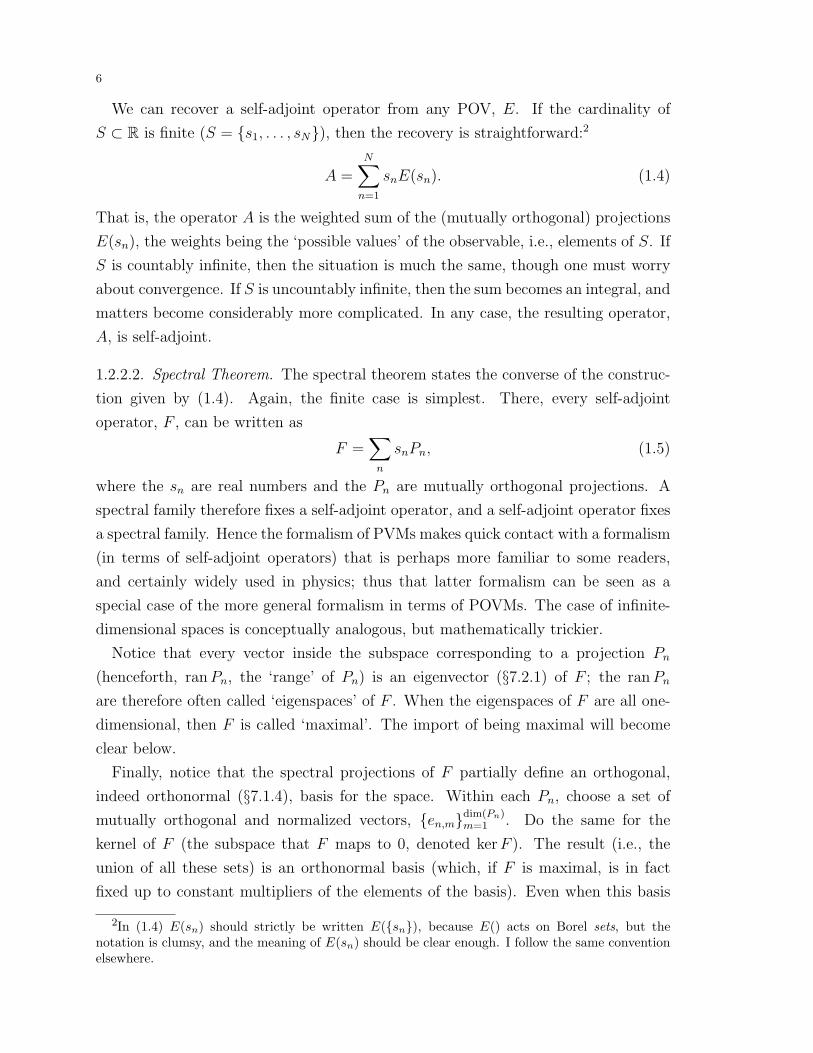
1.2.2.2. Spectral Theorem. The spectral theorem states the converse of the construc-

tion given by (1.4). Again, the finite case is simplest. There, every self-adjoint

operator, F , can be written as

F =∑

n

snPn, (1.5)

where the sn are real numbers and the Pn are mutually orthogonal projections. A

spectral family therefore fixes a self-adjoint operator, and a self-adjoint operator fixes

a spectral family. Hence the formalism of PVMs makes quick contact with a formalism

(in terms of self-adjoint operators) that is perhaps more familiar to some readers,

and certainly widely used in physics; thus that latter formalism can be seen as a

special case of the more general formalism in terms of POVMs. The case of infinite-

dimensional spaces is conceptually analogous, but mathematically trickier.

Notice that every vector inside the subspace corresponding to a projection Pn

(henceforth, ranPn, the ‘range’ of Pn) is an eigenvector (§7.2.1) of F ; the ranPn

are therefore often called ‘eigenspaces’ of F . When the eigenspaces of F are all one-

dimensional, then F is called ‘maximal’. The import of being maximal will become

clear below.

Finally, notice that the spectral projections of F partially define an orthogonal,

indeed orthonormal (§7.1.4), basis for the space. Within each Pn, choose a set of

mutually orthogonal and normalized vectors, {en,m}dim(Pn)m=1 . Do the same for the

kernel of F (the subspace that F maps to 0, denoted kerF ). The result (i.e., the

union of all these sets) is an orthonormal basis (which, if F is maximal, is in fact

fixed up to constant multipliers of the elements of the basis). Even when this basis

2In (1.4) E(sn) should strictly be written E({sn}), because E() acts on Borel sets, but thenotation is clumsy, and the meaning of E(sn) should be clear enough. I follow the same conventionelsewhere.

7

is not uniquely fixed by F (because it is non-maximal), I will refer to such a basis as

‘a basis determined by F ’.

1.2.3. States.

1.2.3.1. Probabilities. The formalism in terms of POVMs (as well as the special case

of PVMs) describes a probabilistic theory, inasmuch as it provides probabilities for

(Borel sets of) values of observables, or (equivalently and sometimes more conve-

niently) expectation values for observables. I will take probabilities as fundamental;

expectation values can then be generated from a probability measure over the possible

values, fn, of F in the usual way:

Exp(F ) = f1 Pr(f1) + f2 Pr(f2) + · · · . (1.6)

As we noticed above, rather than considering directly the possible values of an ob-

servable, we can also consider the corresponding (spectral) projectios, which can be

taken, in a given physical situation, to represent those values.

A probability measure, p, defined on the projection operators should, minimally,

be such that p(P1 + P2) = p(P1) + p(P2) whenever P1⊥P2. (Later I will motivate

this condition. The basic idea is that it corresponds to the usual ‘additivity axiom’

of Kolmogorovian probability theory—see §7.5.6.) More specifically, and for now

considering just the case of PVMs, we require a probability measure on the projections

on a Hilbert space to be a map, p, from projections to the interval [0, 1], where p is

countably additive on sets of mutually orthogonal projections.

Precisely what one means by countable additivity for the operators that are in the

image of a POVM (rather than a PVM) is a slightly subtle matter. In particular, in

general the operators in the image of a POVM—normally they are called ‘effects’—do

not correspond to subspaces, and the notion of orthogonality does not apply. However,

there is a natural generalization of the concept. Notice that for projections, {Pi}, in

the image of a PVM, the condition that I−∑

i Pi be a projection (or maybe the zero

operator) is equivalent to the condition that the {Pi} be mutually orthogonal.3 The

analogous condition in the case of positive operators is that, for effects {Ei} in the

image of a POVM, if I−∑

iEi is positive (or 0), then Pr(∑

iEi) =∑

i Pr(Ei).

1.2.3.2. Statevectors and Wavefunctions.

3Sketch of a proof: Write (I −∑

i Pi)(I −∑

i Pi); expand; argue that if the {Pi} are mutuallyorthogonal, then the result is I −

∑i Pi; argue (using the fact that projections are positive—this

part is less trivial) that if the result is I −∑

i Pi, then the {Pi} are mutually orthogonal; finally,argue that I−

∑i Pi is self-adjoint.

8

1.2.3.2.a. Statevectors. Normalized vectors determine probability measures over the

projections, via:

probability of P as given by v := Prv(P ) := 〈v, Pv〉. (1.7)

(One often sees the expression |〈φ, v〉|2, where φ is a normalized vector from ranP .

The two expressions are equivalent.) Notice that the probabilities generated by the

vectors v and eiφv (where φ is a real number) are the same. One says that ‘overall

phases do not affect probabilities’. The expectation value of a self-adjoint operator,

F , given by the state v is

expectation of P as given by v := Expv(F ) := 〈v, Fv〉. (1.8)

(Note that the expectation value of a projection is also its probability.)

Note that if v ∈ ranP then Prv(P ) = 1. More generally, if Pn is an eigenspace

of F corresponding to the eigenvalue fn and v ∈ ranPn, then Prv(Pn) = 1, i.e. the

probability (in the state v) that F has the value fn is 1. Such a state, v, is called

an ‘eigenstate’ of F—it is a normalized vector inside the eigenspace, ranPn, of F .

Notice that, in this case, writing F in terms of its spectral decomposition (recall 1.4)

makes the determination of probabilities and expected values trivial. Indeed, even

when dealing with general states, it is often convenient to write F in terms of its

spectral decomposition, and the state in terms of a basis determined by F .

1.2.3.2.b. Superposition. It is a standard assumption of quantum theory that every

vector in the Hilbert space for a system is a possible state for the system. This

assumption is often expressed as the ‘superposition principle’, which asserts that

(normalized) linear combinations of statevectors are again statevectors.

Given an observable, F , the superposition principle gives rise to (possible) states

that are not eigenstates of F . Suppose, for simplicitly, that F is maximal, with

eigenspaces and eigenvalues {Pn} and {fn}, and consider an orthonormal basis, {vn},determined by F (which, because F is maximal, just amounts to choosing one nor-

malized vector from each ranPn). Now form the state vector

v =∑

n

kn|vn〉 (1.9)

where∑

n |kn|2 = 1 and with at least two non-zero coefficients kn. In this case, we

say that v is a superposition of the vn. (One sometimes here the word ‘superposition’

used in a way that suggests that some vectors are ‘in superpositions’ and others are

not. Relative to a given basis, this distinction makes sense, but otherwise it does not.

Every vector is a superposition for some choices of basis.) Notice that v is not an

eigenstate of F , and assigns non-trivial probabilities to more than one possible value

9

of F . Of course, the superposition principle implies that v is nonetheless a possible

state of a system.

1.2.3.2.c. Wavefunctions. Wavefunctions are just a specific way of representing stat-

evectors. It is often convenient to take the Hilbert space for a quantum system to

be the elements of L2(R3), in which case statevectors are (equivalence classes of)

complex-valued functions on R3. The equation of motion that they standardly sat-

isfy is a type of wave equation (e.g., the Schrodinger equation—see §1.5.2.3.a), and

for this reason—as well as the fact that the equation was historically derived with

wave phenomena in mind—these functions are called ‘wavefunctions’. Linear combi-

nations of waves may be conceived in terms of ‘superposing’ the waves—hence the

term ‘superposition’.

1.2.3.3. Gleason’s Theorem. One can generate probability measures using non-negative

trace-1 operators (‘density operators’). The functional Tr[·] is the ‘trace functional’,

a map from the bounded operators on a Hilbert space to R defined by:

Tr[F ] =∑

k

〈ek, (F∗F )1/2ek〉 (1.10)

where {ek} is an orthonormal basis for H. (Note that F ∗F is self-adjoint and positive.

It is in fact true that every positive operator, A, has a positive self-adjoint square

root, B, defined by B2 = A.) And if F itself is positive, then F =√F 2 and

Tr[F ] =∑

k

〈ek, Fek〉. (1.11)

The trace functional is provably independent of the choice of orthonormal basis, {ei}.Moreover, a very useful property of the trace functional is that it is invariant under

cyclic permutations of its arguments; for example,

Tr[ABC] = Tr[BCA] = Tr[CAB] (1.12)

for any A,B,C.

Let W be any positive operator on a Hilbert space, H, with Tr[W ] = 1. Let E() be

any POVM from some ‘spectrum’, S, of possible values to positive operators. Then

Tr[WE(·)] is a countably additive probability measure on (the σ-algebra of Borel sets

of) possible values of the observable represented by the POVM E as follows:

Pr(∆) = Tr[WE(∆)]. (1.13)

Countable additivity follows from (1.3) and the linearity of the trace functional. Nor-

malization follows from (1.2) and the fact that W has unit trace.

10

When E(·) is a PVM, (1.13) defines a countably additive normalized measure on

the projections on H. Hence any density operator generates such a measure. The

converse is (remarkably) true as well: every probability (i.e., countably additive,

normalized) measure on the projections on a Hilbert space is generated as in (1.13)

by some density operator. This theorem is due to Gleason (1957), and says, more

precisely:

Theorem (Gleason): Let H be a Hilbert space of dimension greater

than 2. Then every countably additive normalized measure, Pr(·), on

the projections on (equivalently, closed subspaces of) H is generated by

some trace-1 positive operator, W , on H; for P a projection,

Pr(P ) = Tr[WP ]. (1.14)

The proof is non-trivial. Gleason’s theorem is generalizable to the case of general

POVMs. That is, the countably additive probability measures over effects are also

given by the density operators. (Indeed, for POVMs, there is no restriction to the

case dim(H) > 2. Again, the proofs are non-trivial. See Busch (2003).)

In this common understanding of quantum theory, then, the kinematics of a quan-

tum system is, at its core, given by the POVMs on a Hilbert space together with

a state, a density operator. In many cases of interest, one deals with PVMs, hence

self-adjoint operators, rather than with POVMs.

Note, finally, that for any statevector, v, we can always represent v in terms of

the density-operator formalism, by choosing as the state the projection, Pv, onto the

subspace spanned by v. In this case, for any projection Q, Tr[PvQ] = 〈v,Qv〉. (To

prove: take the trace in an orthonormal basis containing v.)

1.2.3.4. Matrix Representation of States. A vector—and in particular a statevector,

ψ—can, of course, be written in terms of any orthonormal basis, {en}, and in this

case, the coefficients cn in the expansion ψ =∑

n cnen may be considered as the

‘coordinates of ψ in the en-basis’. It is, in fact, sometimes convenient (see, e.g.,

§1.3.3.2) to write the state as a column vector with these coordinates.

A similar construction is available for density operators. Again in the (orthonormal)

basis {en}, consider a matrix whose elements are 〈en, Fem〉, for any operator, F , on

a Hilbert space, H. This map from operators on H to N × N matrices (where N

could be infinite) is in fact an isomorphism from the (algebra of) operators on H to

the (algebra of) N ×N matrices

In particular, let W be a density operator on H, and let Wnm = 〈en, Fem〉. Now

let F be an observable whose eigenvectors are the en. Notice, in this case, that

11

〈en, Fem〉 = δnm. One says that F is ‘diagonal’ in the basis {en} (because all of the

entries off of the diagonal are 0). If W is also diagonal in {en, then the probabilities

assigned by W to F behave completely classically, and in particular the classical ‘sum

rule’ holds:

PrW

(fn or fm) = PrW

(fn) + PrW

(fm) (1.15)

(where PrW is the probability assigned by W via 1.14 and fn is the eigenvalue of F

corresponding to the eigenvector en). However, if W is not diagonal in {en}, then in

general (1.15) fails. In this case, one speaks of ‘interference’ between the en (in the

state W ).

1.2.3.5. Expectation Values. It follows immediately that the expectation value of the

observable (represented by the self-adjoint operator) F in the state (represented by

the density operator) W is Tr[WF ]. To see why, write F in terms of its spectral

resolution. The point is most easily seen when F has only a discrete spectrum, as in

(1.5). Then by the linearity of the trace,

Tr[WF ] =∑

n

Tr[WPn]sn. (1.16)

(When F has a continuous spectrum, one must work with integrals whose definition

must be treated carefully.) Notice that the expression Tr[WPn] is the probability

(in state W ) that F takes the value sn. Hence (1.16) is a weighted sum of the

possible (spectral) values, sn, for F , the weights given by the probabilities, Tr[WPn],

associated to those values in the state W . Note that the traces in (1.16) will in general

be easiest to calculate in a basis determined by F .

1.2.3.6. Quantum Probability Theory. Classical probability theory standardly con-

cerns measures over sigma-algebras of events (§7.5.5, §7.5.6). These sigma-algebras

are defined in terms of the usual set-theoretic operations of complement and union.

In quantum theory, we are dealing with a different structure. However it is sufficiently

analogous to the structure considered in the classical setting that, mathematically at

least, one can often easily carry over considerations from classical probability theory.

Our ‘sample space’ is the set of all one-dimensional projections. Set-theoretic com-

plement (E ′) becomes ‘orthogonal complement’ (E⊥); set-theoretic union (E ∪ F )

becomes ‘span’ (the span of the subspaces E and F , written E ∨ F ); set-theoretic

intersection (E ∩ F ) remains intersection (now written E ∧ F ); and set-theoretic ‘in-

clusion’ (E ⊆ F ) becomes subspace inclusion (often written E ≤ F ). Later, I will

consider this structure in more detail—it is the ‘lattice’, L, of subspaces of a Hilbert

space (§7.4). For now, I simply note that it has the correct properties: (i) H ∈ L, (ii)

12

E ∈ L implies E⊥ ∈ L; and (iii) for any countable sequence, {Ek} ∈ L, ∨kEk ∈ L.

Analogous to classical probability theory, quantum probability theory is then the

theory of normalized measures on such a structure. (Of course, if we are thinking in

terms of POVMs rather than PVMs, then this story cannot be told, at least not in its

present form. Instead, one considers the algebra of effects, and probability measures

over it. However, I will not pursue the details here.)

1.2.3.7. Luder’s Rule. What about conditional probabilities? Although its interpre-

tation can be highly contentious, and its application somewhat tricky, there is a

standard expression for a conditional probability in quantum theory, called ‘Luder’s

Rule’. Indeed, one can derive it from elementary considerations.

Recall from basic probability theory that the conditional probability, Pr(A|B), of

one event, A, given another, B, is defined by

Pr(A|B) :=Pr(A ∩B)

Pr(B). (1.17)

The thought behind this definition is that the probability of A (and B) given B

is the probability that A and B occur jointly, ‘renormalized’ under the assumption

that B occurred; i.e., it is the probabilty of A ‘as if’ B had probability 1. Indeed,

(1.17) is the only probability measure that satisfies the condition that if A ⊆ B then

Pr(A|B) = Pr(A)/Pr(B). In other words, if A is contained in B, then Pr(A|B) is just

a renormalization of the original probability measure to one that assigns probability

1 to B.

It turns out that this condition is already sufficient to determine the form of the

conditional probability measure over the (lattice of) closed subspaces of (or projec-

tions on) a Hilbert space (Bub 1977). In other words, let PrW be the probability

measure associated with the density operator, W , on H. Let P be a subspace such

that PrW (P ) 6= 0 (where, of course, PrW (P ) = Tr[WP ]). Then there is a unique

probability measure, PrW |P (the ‘probability in state W conditional on P ’), over the

closed subspaces of H such that

PrW |P (Q) := PrW (Q|P ) =PrW (Q)

PrW (P )(1.18)

for any Q ≤ P . That measure is given by

PrW (Q|P ) =Tr[PWPQ]

Tr[WP ]. (1.19)

(1.19) is known as ‘Luder’s Rule’. Note that for a statevector, |v〉, the same effect is

achieved by projecting |v〉 onto P , normalizing the result, and using that new state

13

(P |v〉/||Pv||) to calculate the probability of Q. Hence (using eq. 1.7)

Pr|v〉(Q|P ) = 〈Pv|QPv〉/||Pv||2. (1.20)

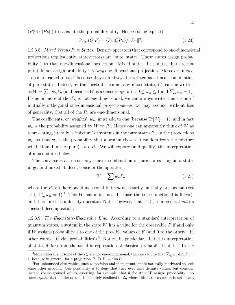
1.2.3.8. Mixed Versus Pure States. Density operators that correspond to one-dimensional

projections (equivalently, statevectors) are ‘pure’ states. These states assign proba-

bility 1 to that one-dimensional projection. Mixed states (i.e., states that are not

pure) do not assign probabilty 1 to any one-dimensional projection. Moreover, mixed

states are called ‘mixed’ because they can always be written as a linear combination

of pure states. Indeed, by the spectral theorem, any mixed state, W , can be written

as W =∑

nwnPn (and because W is a density operator, 0 ≤ wn ≤ 1 and∑

nwn = 1).

If one or more of the Pn is not one-dimensional, we can always write it as a sum of

mutually orthogonal one-dimensional projections—so we may assume, without loss

of generality, that all of the Pn are one-dimensional.

The coefficients, or ‘weights’, wn, must add to one (because Tr[W ] = 1), and in fact

wn is the probability assigned by W to Pn. Hence one can apparently think of W as

representing, literally, a ‘mixture’ of systems in the pure states Pn, in the proportions

wn, so that wn is the probability that a system chosen at random from the mixture

will be found in the (pure) state Pn. We will explore (and qualify) this interpretation

of mixed states below.

The converse is also true: any convex combination of pure states is again a state,

in general mixed. Indeed, consider the operator

W =∑

n

wnPn (1.21)

where the Pn are here one-dimensional but not necessarily mutually orthogonal (yet

still,∑

nwn = 1).4 This W has unit trace (because the trace functional is linear),

and therefore it is a density operator. Note, however, that (1.21) is in general not its

spectral decomposition.

1.2.3.9. The Eigenstate-Eigenvalue Link. According to a standard interpretation of

quantum states, a system in the state W has a value for the observable F if and only

if W assigns probability 1 to one of the possible values of F (and 0 to the others—in

other words, ‘trivial probabilities’).5 Notice, in particular, that this interpretation

of states differs from the usual interpretation of classical probabilistic states. In the

4More generally, if some of the Pn are not one-dimensional, then we require that∑

n wn dimPn =1, because in general, for a projection P , Tr[P ] = dimP .

5For unbounded observables, such as position and momentum, one is naturally motivated to seeksome other account. One possibility is to deny that they ever have definite values, but considerinstead coarse-grained values, asserting, for example, that if the state W assigns probability 1 tosome region, ∆, then the system is definitely confined to ∆, where this latter assertion is not meant

14

classical case, the probabilistic state is a measure over possible pure states, and one

normally presumes that the system really is in one of those pure states.

This rule for assigning definite values has come to be called, following Fine (1973),

the ‘eigenstate-eigenvalue link’. Later (§5) we will consider in some detail the apparent

consequences of this rule.

1.2.4. Incompatibility. An immediate consequence of this formalism is the fact that

there are ‘incompatible’ physical quantities, at least in the minimal sense that if a

state assigns probability 1 to some physical quantity (some projection, for example),

then it necessarily assigns non-trivial probabilities (i.e. neither 0 nor 1) to others (and

then, by the eigenstate-eigenvalue link, these other observables do not have values, in

that state—recall §1.2.3.9). This fact follows directly from Gleason’s theorem. (Note,

however, that one can show in other, simpler, ways that there are no two-valued

probability measures over the projections on a Hilbert space.)

Incompatibility is closely related to non-commutativity, and indeed the two terms

are sometimes used interchangeably. Consider two projection operators, Q and Q′.

To keep things simple, we will suppose throughout that Q and Q′ are one-dimensional.

Then if Q and Q′ do not commute, i.e., [Q,Q′] 6= 0, there is no state that assigns

probability 1 to Q and either 0 or 1 to Q′. To prove this claim, we will first show

(next paragraph) that the only state assigning probability 1 to a one-dimensional

projection, Q, is the state Q itself. (Notice that in the previous sentence, the first

mention of Q is as the representative of some physical quantity, and the second is

as a state.) We will then show (subsequent paragraph) that Q assigns non-trivial

probabilities to any non-commuting Q′.

Let W be a state that assigns probability 1 to (one-dimensional) Q. Writing W

in terms of its spectral decomposition, and taking the trace in a basis determined by

W , we immediately find that

Tr[WQ] =∑

n

wn〈en, Qen〉 = 1 (1.22)

where the weights wn (from the spectral decomposition of W ) sum to 1. Hence for

some n, Qen = en, i.e., W is in fact pure, and equal to Q. Therefore, the only state

assigning probability 1 to a one-dimensional projection, Q, is Q itself.6

to imply that there is some point in ∆ that is the location of the system. There are, however, otherapproaches. See, for example, Halvorson (2001).

6This claim is also true in a more general form. Let the state W assign probability 1 to theprojection Q (of any dimension). Then (ranQ)⊥ ⊆ ker(W ), with equality if Q is the smallestsubspace to which W assigns probability 1.

15

Now suppose that (one-dimensional) Q′ 6= Q and Q′ 6⊥Q, i.e., Q and Q′ do not com-

mute (for a discussion, see below). Then, by the same reasoning as above, replacing

Q with Q′ in (1.22), if Tr[WQ′] = 1 then W must be pure and lie inside the subspace

associated with Q′; i.e., W = Q′. But it cannot, because we assumed that Q 6= Q′.

On the other hand, if we want Tr[WQ′] = 0, then kerW ⊆ ranQ′. (The reasoning is

essentially the same as above.) But again it cannot, because then Q′⊥Q, given our

earlier conclusion that W is pure and lies in the subspace associated with Q, and we

already assumed that Q′ 6⊥Q.

This fact is also true in a more general form. Given two self-adjoint operators, F and

G, if F and G do not share any eigenvectors then any state that assigns probabiltiy

1 to some value for F will necessarily assign non-trivial probabilities (neither 0 nor

1) to more than one of the possible values of G. I leave the proof (using essentially

the same reasoning as above) to the reader.

Above I claimed that (one-dimensional) Q and Q′ do not commute if Q′ 6= Q

and Q′ 6⊥Q. In fact, the following is true. For any subspaces, A and B, and the

corresponding projections PA and PB, [PA, PB] = 0 if and only if

A = (A ∧B) ∨ (A ∧B⊥) and B = (B ∧ A) ∨ (B ∧ A⊥). (1.23)

(Here we are not restricting to one-dimensional subspaces. Note, however, that (1.23)

is implied by the disjunction ‘A = B or A⊥B’, and for one-dimensional subspaces,

they are equivalent.) Here is the idea of the proof. Note that A ∧ B and A ∧ B⊥

are orthogonal. Hence, if (1.23) holds, we may write PA = PZ + PA′ for some Z⊥A′.(Indeed, of course, Z = A∧B and A′ = A∧B⊥.) Similarly, PB = PZ+PB′ , withB′⊥Z.

Moreover, A′⊥B′. In other words, the conditions (1.23) imply that A and B ‘are

orthogonal apart from some shared part (Z)’. Then [PA, PB] = [PZ +PA′ , PZ +PB′ ] =

[PZ , PZ ] + [PZ , PB′ ] + [PA′ , PZ ] + [PA′ , PB′ ] = 0.

Going the other way, we will just sketch the idea. If PA and PB commute, then

for any vector, v, PAPBv = PBPAv. First choose v ∈ A, so that PAPBv = PBv. In

general, if PAw = w (here w = PBv), then either w ∈ A or w = 0. Hence either (i)

PBv = 0, or (ii) PBv ∈ A. If (i) is true for all v ∈ A, then B⊥A and (1.23) clearly

holds. If (ii) holds for all v ∈ A then B ≤ A and again (1.23) clearly holds. Using

the linearity of the operators involved, one can show that if (ii) holds for just some

v ∈ A, then the PBv must form a subspace of A, and clearly this subspace is common

to A and B; indeed it is A ∧ B. Similarly, one can show that choosing v from the

subspace orthogonal to A∧B gives rise to (i), so that indeed A = (A∧B)∨ (A∧B⊥).

Repeating the argument for v ∈ B, we find that (1.23) holds.

16

The fact of incompatibility marks a significant departure from classical physics,

where the structure of the space of states and observables allows for states that as-

sign values to all observables with probability 1 (i.e., there are two-valued probability

measures over the space of all ‘properties’ of the system). The probabilities of quan-

tum theory appear, therefore, to be of a fundamentally different character from the

probabilities of classical theory, which arise always because the state of the system is

not maximally specific.7

1.2.5. Canonical Commutation Relations. An important and classic example of in-

compatibility involves the position and momentum observables. In fact, they obey

the ‘canonical commutation relations’ (CCRs):

[Pi, Qj] = −iδij (1.24)

where i and j can be x, y, or z. (Henceforth, we will restrict our attention to one

dimension, writing [P,Q] = −i. The generalization to three dimensions is straightfor-

ward.) Note that the constant on the right-hand side implicitly multiples the identity

operator.

Any two observables that obey these commutation relations are typically called

‘canonically conjugate’. These relations are central in quantum theory, and we will

discuss them in detail in §4. For now, we simply notice them as a central example of

incompatibility.

1.2.6. Compound Systems.

1.2.6.1. Entangled States. Compound systems are represented by tensor-product Hilbert

spaces (§7.1.9), so that, for example, a system composed of two particles has a state

that is a density operator on the tensor-product of the Hilbert spaces for the two par-

ticles individually. There is a fundamental and physically crucial distinction between

two kinds of vector in H = H1⊗H2. A vector, v, in H is called ‘factorizable’ if it can

be written as x ⊗ y for some x ∈ H1 and y ∈ H2. Otherwise, v is called ‘unfactor-

izable’, or ‘entangled’. An analogous definition applies to the operators (hence, the

density operator states) on H.

The existence of entangled states (whether represented as density operators or

vectors) turns out to have numerous interesting consequences. It is connected with

7Here we are considering just cases where classical physics delivers genuine probability measures,and we ignore cases where classical physics is simply indeterminate. See Earman, Ch. 15, thisvolume.

17

‘quantum-nonlocality’, as well as the possibility of certain computational and information-

theoretic (for example, cryptographic) feats that cannot be done with classical sys-

tems.8 The existence of these states follows from the demand that the pure (vector)

states for the compound system be closed under taking linear combinations. In other

words, it follows from applying the superposition principle to compound systems as

well as to simple systems.

1.2.6.2. Bi-orthogonal Decomposition. An important result about vectors in tensor-

product spaces is the ‘bi-orthogonal decomposition theorem’ (Schrodinger 1935b),

which states that, given a vector, v, in a Hilbert space, H, and a factorization of Has H = H1⊗H2, there exist orthonormal bases {en} of H1 and {fm} of H2 such that

v =∑

n

cn(en ⊗ fn). (1.25)

If the |cn| 6= |c′n| for all n 6= n′, then the bases are unique (up to a phase eiθ on each

element of the basis). Note that, in general, for arbitrary bases {xn} and {ym} of H1

and H2, v is expressed in general in terms of a double sum:

v =∑n,m

cnm(xn ⊗ ym) (1.26)

and compare this expression with (1.25).

1.2.6.3. Reduced States.

1.2.6.3.a. Partial Trace and the Reduced Density Operator. Suppose we are given

the state of a compound system, and wish to derive from it a state for one of the

components. If the compound state is factorizable, then the procedure is straight-

forward. (The state W = W1 ⊗ W2 fixes the component states to be W1 and W2

respectively.) But what about when it is entangled? Here we face a problem. If the

state is entangled, then there is no obvious sense in which it can be ‘divided’ into a

‘part’ corresponding to one system, and a ‘part’ corresponding to the other.

The usual solution to this problem is to take the state of the component systems to

be given by a partial trace. For any tensor-product Hilbert space, H = H1 ⊗H2, the

‘partial trace over H1’ is a map, tr(1)[·], from the operators on H to operators on H2.

It is the unique such map satisfying the condition that, for any density operator W on

H and any observable F2 on H2, the operator tr(1)[W ] generates the same expectation

value for F2 as W does for I1⊗F2 (Jauch 1968, §11-8). The idea is that tr(1)[·] ‘traces

out’ system 1, extracting just that part of the compound state that applies to system

8See Bub, Ch. 6, this volume.

18

2. Unless W is a ‘product state’ (i.e., W = W1 ⊗W2), the reduced states derived

from W are necessarily mixed states.

1.2.6.3.b. Proper Versus Improper Mixtures. In §1.2.3.8 I introduced the idea that a

mixed state can be understood as a literal mixture of systems each in some pure state.

Certainly when we are describing the state of a system chosen at random from an

ensemble that was produced by literally ‘mixing’ systems in various pure states, it is

quite proper to interpret the mixed state in this way. However, we now see that mixed

states can arise in another way, namely, as the state of one component of a compound

system that is in a non-factorizable compound state. In these cases, it is far from

clear that the state (of the component) should be understood as above. Indeed, there

need not even be an ensemble of which this component is a part. Hence mixtures that

arise from taking the partial trace of the state of a compound system are normally

called ‘improper mixtures’, while those that arise from a mixing of individual systems

in pure states are normally called ‘proper mixtures’ (a terminology introduced by

dEspagnat §1971). Whether the probabilities generated by improper mixtures can

reasonably be understood as ‘ignorance about the true pure state’ (as they can for

proper mixtures) is a matter for interpretative investigation.

1.2.6.4. Correlations. Compound systems that are in a non-factorizable state will

exhibit correlations between the measured values of observables on the two (or more)

components. Consider, for example, the statevector v = c1f1⊗g1+c2f2⊗g2 (where c1

and c2 are non-zero coefficients), and suppose that the fn and the gn are eigenvectors

of the observables F and G respectively. In this state, there is a correlation between

the value of F on system 1 and G on system 2. Indeed, let Pfn and Pgn be the

projections onto the subspaces spanned by fn and gn respectively, and let Pv be the

projection onto the subspace spanned by v. Then, applying Luder’s Rule (1.19), we

find

PrPv(I1 ⊗ Pgn′|Pfn ⊗ I2) =

Tr[(Pfn ⊗ I2)Pv(Pfn ⊗ I2)(I1 ⊗ Pgn′)]

Tr[Pv(I1 ⊗ Pfn)](1.27)

where Ik is the identity on Hk. Taking the trace in a basis that includes the fn ⊗ gn′

reveals that this conditional probability is 0 when n 6= n′ and 1 when n = n′. In other

words, the values of F (on system 1) and G (on system 2) are perfectly correlated.9

9Authors will sometimes say that two observables are ‘perfectly anti-correlated’ if the two observ-ables have the same spectrum and the value of one is always minus the value of the other. Theywill also occasionally reserve the term ‘perfect correlation’ for a similar case, where the value of oneis always equal to the value of the other. Our use of the term ‘perfect correlation’—according towhich two observables are perfectly correlated in a state just in case the conditional probabilitiesfor values of one, given a value of the other, are always 0 or 1—covers both cases.

19

Consideration of other observables would reveal additional correlations (not always

perfect correlations). We will see an example later.

1.2.7. Structure of the Space of States. We noted above (§1.2.3.8) that every convex

combination of pure states is again a state. Of course, a convex combination of mixed

states is (by the spectral theorem) also a convex combination of pure states, so that

in fact the set of states forms a convex set (§7.1.10), a point that I shall discuss in

detail later (§2.2.1). Here we note the fundamental point that the convex set of states

in quantum theory is not a simplex.

This point marks a departure from classical physics, where every mixed state is

uniquely decomposable in terms of pure states. One thus naturally takes the mixed

state as a measure of ignorance over the pure states that appear in its decomposition.

No correspondingly straightforward interpretation of mixed states in quantum theory

is available, in part because the mixed states are multiply decomposable into a convex

combination of pure states.

1.3. Simple Example: A Spin-12

Particle. An understanding of the formalism,

and the issues to which it gives rise, is much aided by some experience with actual

calculations, however simple. In that spirit, let us consider the example of a spin-12

particle. The example is well-worn, but deservedly so. While there are some impor-

tant foundational and philosophical issues concerning quantum theory that cannot

be illustrated or investigated in the context of spin-12

particles, many such issues can

be investigated in this context.

1.3.1. Introduction of Spin into Quantum Theory. Spin was introduced in 1924 in the

course of an attempt to understand the spectrum of electromagnetic radiation emitted

by certain metals. In the course of that explanation, electrons were supposed to have

some “two-valued quantum degree of freedom”.10 This degree of freedom was soon

associated with a rotation of the electron. Because the electron is a charged body,

its rotation creates a magnetic field—the electron acts as a magnet whose north and

south poles lie on the axis of rotation. This magnetic property was just what was

needed to explain the phenomena.

So far, the story sounds good. However, it was seen almost immediately that the

rotation cannot be literal. Nonetheless, the theory of ‘spin’ was developed in the

context of the new quantum theory; the name stuck, and we continue to refer to

this magnetic property of electrons (and as current theory tells us, other particles) as

‘spin’.

10See Massimi (2004, chs. 2,4) for discussion.

20

N

S

sourcemagnets

photographic plate

Figure 1. An experiment involving Stern-Gerlach magnets

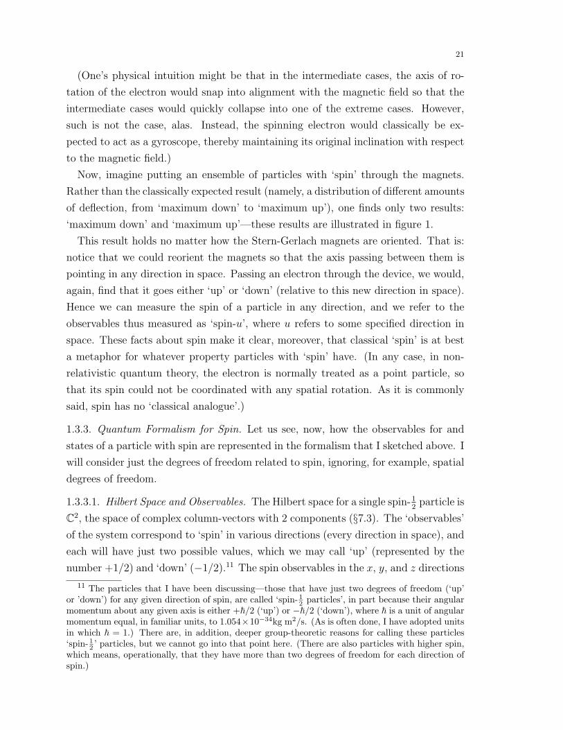
1.3.2. Quantization of Spin. It turns out that spin is ‘quantized’, a fact already antic-

ipated in Pauli’s characterization of the property as a ‘two-valued degree of freedom’.

This fact is, classically, unexpected. To see why, consider a standard method for mea-

suring the spin of a particle. (The method does not, in fact, work for electrons, but it

illustrates the point well enough, and does work for electrically neutral particles with

spin.) The relevant device is a ‘Stern-Gerlach’ device, a pair of magnets shaped and

arranged to create an inhomogeneous magnetic field, that is, a magnetic field that is

stronger in one direction (say, the north) than in the other. (See figure 1.)

Imagine a simple bar magnet passing between the Stern-Gerlach magnets. If the

north pole points straight up so that it is close to the top magnet, then the top

magnet pushes the north pole (of the bar magnet) down more than the bottom

magnet pushes the south pole up, and the net result will be that the bar magnet

is deflected downward. If the bar magnet enters the Stern-Gerlach magnets with the

south pole facing up, then the result is the opposite: overall upward deflection. If,

on the other hand, the bar magnet enters the Stern-Gerlach magnets horizontally,

then it will pass straight through with no overall deflection in its path. Finally, if

the bar magnet passes through neither vertically nor horizontally, then the result

will be deflection, up or down, that is somewhere between the extreme cases. (The

trajectories of the magnet in the two extreme cases are illustrated in figure 1.)

21

(One’s physical intuition might be that in the intermediate cases, the axis of ro-

tation of the electron would snap into alignment with the magnetic field so that the

intermediate cases would quickly collapse into one of the extreme cases. However,

such is not the case, alas. Instead, the spinning electron would classically be ex-

pected to act as a gyroscope, thereby maintaining its original inclination with respect

to the magnetic field.)

Now, imagine putting an ensemble of particles with ‘spin’ through the magnets.

Rather than the classically expected result (namely, a distribution of different amounts

of deflection, from ‘maximum down’ to ‘maximum up’), one finds only two results:

‘maximum down’ and ‘maximum up’—these results are illustrated in figure 1.

This result holds no matter how the Stern-Gerlach magnets are oriented. That is:

notice that we could reorient the magnets so that the axis passing between them is

pointing in any direction in space. Passing an electron through the device, we would,

again, find that it goes either ‘up’ or ‘down’ (relative to this new direction in space).

Hence we can measure the spin of a particle in any direction, and we refer to the

observables thus measured as ‘spin-u’, where u refers to some specified direction in

space. These facts about spin make it clear, moreover, that classical ‘spin’ is at best

a metaphor for whatever property particles with ‘spin’ have. (In any case, in non-

relativistic quantum theory, the electron is normally treated as a point particle, so

that its spin could not be coordinated with any spatial rotation. As it is commonly

said, spin has no ‘classical analogue’.)

1.3.3. Quantum Formalism for Spin. Let us see, now, how the observables for and

states of a particle with spin are represented in the formalism that I sketched above. I

will consider just the degrees of freedom related to spin, ignoring, for example, spatial

degrees of freedom.

1.3.3.1. Hilbert Space and Observables. The Hilbert space for a single spin-12

particle is

C2, the space of complex column-vectors with 2 components (§7.3). The ‘observables’

of the system correspond to ‘spin’ in various directions (every direction in space), and

each will have just two possible values, which we may call ‘up’ (represented by the

number +1/2) and ‘down’ (−1/2).11 The spin observables in the x, y, and z directions

11 The particles that I have been discussing—those that have just two degrees of freedom (‘up’or ’down’) for any given direction of spin, are called ‘spin- 1

2 particles’, in part because their angularmomentum about any given axis is either +~/2 (‘up’) or −~/2 (‘down’), where ~ is a unit of angularmomentum equal, in familiar units, to 1.054×10−34kg m2/s. (As is often done, I have adopted unitsin which ~ = 1.) There are, in addition, deeper group-theoretic reasons for calling these particles‘spin- 1

2 ’ particles, but we cannot go into that point here. (There are also particles with higher spin,which means, operationally, that they have more than two degrees of freedom for each direction ofspin.)

22

are defined in terms of the Pauli matrices by Sx = (1/2)σx, and similarly for Sy and

Sz. (See §7.3.1).

1.3.3.2. States. The pure states can be represented by norm-1 vectors, or by projec-

tions onto the space spanned by them. Consider, for example, the statevectors

ψ =

(10

), χ =

(01

). (1.28)

The vector ψ, for example, corresponds to the (pure) density operator (one-dimensional

projection operator)

W =

(1 00 0

). (1.29)

The vectors ψ and χ are an eigenvectors of

σz =

(1 00 −1

)(1.30)

with eigenvalues +1 and −1 respectively.

Note that the expectation value of Sz in the state W is

Tr

[(1 00 0

)(12

00 −1

2

)]= Tr

[(12

00 0

)]

= (1 0)

(12

00 0

)(10

)+ (0 1)

(12

00 0

)(01

)= 1

2+ 0 = 1

2.

(1.31)

(Recall our earlier comments about calculating traces in an appropriately chosen

basis.) Of course, in general a system’s having an expectation value equal to some

value, r, is not sufficient to imply that the system has the value r. (Indeed, r might

not even be in the spectrum of possible values.) In this case, however, we may also

note that the probability associated with the appropriate projection operator is 1.

So, first, note that the spectral decomposition of Sz is:

Sz =

(12

00 −1

2

)=(+1

2

)( 1 00 0

)+(−1

2

)( 0 00 1

):=(+1

2

)Pz+ +

(−1

2

)Pz− .

(1.32)

Hence the projection associated with the value +12

for Sz is Pz+ and the probability

for the value +12

(for Sz) in the state W is

Tr[WPz+ ] = Tr

[(1 00 0

)(1 00 0

)]= 1. (1.33)

(We leave the details of the calculation to the reader. Notice that taking the trace of

a matrix amounts to just adding the numbers along the diagonal. The reader might

23

wish to prove this fact.) As I noted above in a more general context, this expression

is, equivalently, the expectation value of Pz+ in the state W . Hence, in particular,

if one agrees that ‘value r for observable F has probability 1 in state W ’ implies

‘a system in state W has value r for F ’ then we may conclude, from (1.33), that a

system in the state W has the value +1/2 for Sz. (We will discuss such interpretive

principles in more detail later.)

1.3.4. Incompatibility. Finally, notice that in this state, W , the expectation value of

spin in the x and y directions is 0. For example,

Tr[WSx] = Tr

[(1 00 0

)(0 1

212

0

)]= Tr

[(0 1

20 0

)]= 0. (1.34)

This fact suggests (indeed, in this two-dimensional case, implies) that the probabilities

for Sx = +12

and Sx = −12

in the state W are 12, as we can also verify by a direct

calculation. First, note that the spectral resolution of Sx is:

Sx =

(0 1

212

0

)=(

12

)( 12

12

12

12

)+(−1

2

)( 12−1

2

−12

12

):=(+1

2

)Px+ +

(−1

2

)Px− .

(1.35)

As the reader may verify, Tr[WPx+ ] = Tr[WPx− ] = 12.

We have thus verified, in this particular case, a claim made previously made ab-

stractly, namely, that a state that is dispersion-free (i.e., generates probabilties of just

0 or 1 for all possible values) for one observable, will necessarily not be dispersion-

free for some other observables. Indeed, I said earlier that non-commuting observables

that do not share eigenvectors are always incompatible, in the sense that any state

that is dispersion-free on one of them is necessarily not dispersion-free on the other.

Now notice that Sx, Sy, and Sz are mutually non-commuting, and indeed share no

eigenvectors. (In this two dimensional case, non-commuting maximal observables

cannot share any eigenvectors.) Hence a state that is dispersion-free for one will

necessarily generate non-trivial probabilities for the others.

Indeed, consider any direction, u, in space specified relative to the z-axis by the po-

lar angles θ and φ, i.e., in Cartesian coordinates, u = (x, y, x) = (sin θ cosφ, sin θ sinφ, cos θ).

(See Figure 2.) Then the associated spin observable is represented by the matrix

Su =1

2

(cos θ e−iφ sin θeiφ sin θ − cos θ

). (1.36)

24

��

��

��

~z

~uθ

@@

@@φ

Figure 2. Polar angles.

(One reasonable and quick justification of this expression is to note that Su =

Sx sin θ cosφ + Sy sin θ sinφ + Sz cos θ.) The only pairs of such operators that com-

mute are anti-parallel; i.e., they correspond to spin in anti-parallel directions (and

such operators are just multiples of one another by a factor of −1).

(One should keep in mind, however, that Gleason’s theorem does not hold for

our 2-dimensional space. Hence the density operators do not define all states, in

this case. Indeed, Bell (1964) shows how to define a dispersion-free measure over

the projections on C2 in terms of an additional ‘hidden’ parameter. Moreover, the

quantum-mechanical states are obtainable by averaging over the possible values of

the hidden parameters with an appropriate probability distribution over them.)

1.3.5. The Bloch Sphere. The Hilbert space C2 is used to represent any two-level

quantum system, and such systems are of great interest in quantum theory, all the

more so in recent years, as increasing interest in quantum information and quantum

computation has focused attention even more on such systems (because they are the

quantum analog of a classical ‘bit’—see Bub, Ch. 6, this volume). A careful study of

the pure states on C2 is often aided by the representation of those states in terms of

the Bloch sphere. Note that any pure state on C2 can be represented by a vector of the

form v = cos(θ/2)ψ + eiφ sin(θ/2)χ (using the notation of equations 1.28).12 Hence,

again referring to figure 2, we can represent each distinct pure state as a unique point

on the surface of a unit sphere (in R3), normally called the ‘Bloch sphere’. The ‘north

pole’ of the sphere corresponds to the state ψ and the ‘south pole’ to the state χ.

12The claim is not that every vector can be written in this form, but that every pure state canbe represented in this form. Recall that an overall phase factor does not affect the probabilitiesgenerated by a vector. Hence we may assume, without loss of generality, that the coefficient of ψ isreal.

25

In fact, however, the ‘Bloch sphere’ is a ball. The interior points correspond to

mixed states, as follows. Every density operator, W , on C2 can be written as

W =I + ~r · ~σ

2(1.37)

for ~σ the ‘vector’ of Pauli matrices (§7.3.1) and ~r a vector from R3 with ||~r|| ≤ 1.

The components of ~r determine a point inside the Bloch sphere representing the

corresponding density operator. (Note, in particular, that ~r = (0, 0, 1) corresponds

to the pure state given by θ = 0, as it should.)

1.4. Dirac Notation. We will return to the example of a spin-12

particle later to illus-

trate a number of issues in quantum theory. When I do so—and, indeed, throughout

the remainder of this essay—it will be helpful to have at hand a useful notation, the

so-called ‘Dirac bra-ket’ notation, used commonly by both physicists and philoso-

phers.

1.4.1. Bras and Kets. In the bra-ket notation, vectors are denoted by (and sometimes

called) ‘kets’, |v〉. In the discussion above, for example, the column vector ψ in (1.28)

might be denoted |z+〉. Elements of the dual space (the ‘row vectors’ in our discussion

above–see §7.1.8) are denoted by ‘bras’, 〈v|. In our example above, there is a natural

1-1 map from the kets (column vectors) to the bras (row vectors):(ab

)→ (a∗ b∗). (1.38)

The bras thus define (continuous) linear functionals in the obvious way. Letting

|v〉 =

(ab

)and |w〉 =

(cd

), (1.39)

the linear functional (bra) 〈v| acting on the vector (ket) |w〉 is

(a∗ b∗)

(cd

)= a∗c+ b∗d (1.40)

and is written, in the Dirac notation, as (the ‘bra-ket’) 〈v|w〉. (The reader might

wish to check that the functional thus defined is indeed linear.) Of course, as it must

be, 〈v|w〉 is also the inner product of |v〉 with |w〉, given (1.38). (In this notation, we

continue to write ||v|| for the norm of a vector, instead of |||v〉||.)In the general case, i.e. where H is any (complex) Hilbert space (countable-

dimensional at most), we take the elements of H to be kets, and the elements of

the dual space H∗ to be bras. Inner products may now be written 〈v|w〉, which de-

notes both the linear functional |v〉 acting on the vector |w〉 and the inner product of

the vectors |v〉 and |w〉.

26

1.4.2. Operators. The operator, F , acting on the vector |v〉 is written F |v〉. The

expectation value of the observable F in the state |v〉 is written 〈v|F |v〉, which is

notationally (and numerically) equivalent to 〈v|Fv〉, the latter to be read as the inner

product of |v〉 with the vector F |v〉. The expression 〈w|F |v〉 is defined similarly.

Corresponding to what is sometimes called the ‘vector direct product’(ab

)(c d) =

(ac adbc bd

), (1.41)

we can define |v〉〈w| to be the operator on H defined by(|v〉〈w|

)|x〉 = 〈w|x〉 |v〉. (1.42)

Notice that simple symbol-manipulation would generate the same result.

1.4.3. Using the Dirac Notation. As I just hinted, the Dirac notation is enormously

useful, once its true meaning is understood, and dangerous otherwise. It’s power—and

danger—lies in the fact that it allows one more or less to ignore various distinctions,

such as the distinction between a vector and a linear functional (element of a dual

space). It also can be very helpful for ‘coordinate-free’ calculations. For example,

we can discuss the theory of spin-12

particles without bothering with Pauli matrices

and so on. Consider the basis {|z+〉, |z−〉} for C2, where |z+〉 is the state that assigns

probability 1 to the value +12

for Sz and so on—note that we do not need to worry

about how to represent this state as a column of complex numbers. It is sufficient to

carry out calculations to note that for a direction in space, u, specified by the angles

θ and φ relative to the z-axis:

|u+〉 = cos(

θ2

)e−i φ

2 |z+〉+ sin(

θ2

)ei φ

2 |z−〉 (1.43)

|u−〉 = − sin(

θ2

)e−i φ

2 |z+〉+ cos(

θ2

)ei φ

2 |z−〉. (1.44)

The spin observables are then represented by

Su =1

2|u+〉〈u+| −

1

2|u−〉〈u−|. (1.45)

Note, for example, that 〈z+|u+〉 = cos(

θ2

)e−i φ

2 and 〈z−|u+〉 = sin(

θ2

)ei φ

2 , facts that

are immediately read off of (1.43). Hence, for example, the probability that a system

in the state W = |z+〉〈z+| has the value +12

for the observable Su can be quickly

27

calculated as

Tr[|z+〉〈z+|

(|u+〉〈u+|

)](1.46)

= 〈z+|(|u+〉〈u+|

)|z+〉 (1.47)

= 〈z+|u+〉〈u+|z+〉 (1.48)

= |〈z+|u+〉|2 (1.49)

= cos(

θ2

)2. (1.50)

(To get from the first to the second line, calculate the trace using the basis {|z+〉, |z−〉}.)The genuis of Dirac’s notation is that one can, as illustrated here, simply ‘do the sym-

bolically natural thing’ and get the correct answer. For example, the third line follows

from the second by ‘erasing the parentheses and joining the bars’. Conceptually, we

allowed the operator |u+〉〈u+| to act on |z+〉, obtaining the vector 〈u+|z+〉|u+〉, then

took the inner product of this vector with |z+〉 (or, applied the linear functional 〈z+|to 〈u+|z+〉|u+〉). The convenience of the notation can also, however, lead one to forget

conceptually important distinctions.

Keep in mind, moreover, that the convenience of not having to worry about explicit

(e.g., matrix) representations of vectors and observables can also lead one to write

down some rather silly, or at least physically opaque, states. One frequently, for

example, sees written down ‘states’ such as |cat dead〉 or |Sarah sees the pointer〉.The Dirac notation naturally tempts one to write down such expressions, but we are

so far from knowing whether such ‘states’ correspond to some pure vector state, and

if so, what their properties are, that such expressions are best left to cartoons.

1.5. Transformations. We have now seen how to represent observables, and how to

calculate expectation values (and probabilities). While such matters are indeed at the

heart of the theory, there are other aspects of the formalism that are important for

philosophical and foundational discussions. In particular, this subsection discusses

transformations, both of the states of physical systems and of the observables as-

sociated with those systems. Along the way, I will have occasion to mention some

theorems that are fundamental for the foundations of quantum mechanics.

1.5.1. Groups and Their Representations.

1.5.1.1. Motivation. Galileo observed that the laws of motion do not depend on the

constant velocity of the ‘lab’ (frame of reference) in which they are applied. (For ex-

ample, in the hull of a ship moving with constant velocity — more precisely, moving

inertially — “jumping with your feet together, you pass equal spaces in every direc-

tion”, as Galileo writes, just as you would back on shore.) Neither do they depend on

28

one’s location, nor on the time at which they are applied, nor on the direction in which

one is facing. In other words, the laws are invariant under certain transformations,

namely, boosts (changes in velocity), spatial translations, temporal translations, and

rotations. These sorts of transformation are represented, mathematically, by groups,

and in the case of the ‘Galilean transformations’ that I just mentioned, the group

is normally called the ‘Galilean group’.13 Hence group theory (§7.6) is the natural

context in which to study, among other things, the ‘invariances’ of quantum theory.

The motivation here is that the properties of a group are exactly the properties

normally thought to apply to ‘invariance transformations’. In particular, if α and

β are transformations that each individually leave the laws unchanged, then the

composition of α followed by β is also such a transformation. Similarly, if α is

a such transformation, then there is the transformation that ‘undoes’ what α did,

that is the inverse of α. Notice, for example, that the composition of two Galilean

transformations is another one, and that each transformation has an inverse.14

Groups show up in other contexts as well. Suppose, for example, that we are

interested (as we soon will be) in the dynamics of a closed physical system. One way

to think about the time-evolution of the state of a system is as a transformation on

the set of states. The set of all such time-evolutions, then, plausibly should form a

group. The identity represents ‘no change’ (or the degenerate case of evolution over

no time). The product represents one period of evolution followed by another. And

the inverse represents ‘reversed’ evolution, or evolution backwards in time. (If a given

theory is not time-reversible, then we would be dealing with a semi-group rather than

a group.)

Now, often one specifies a group abstractly, that is, by specifying the products

and inverses in the group without representing it as a group of transformations on

some set (such as the set of physical states of a system). The most trivial example

is the group Z2, which contains two elements, x and y. The multiplication rule is:

xy = x, yx = x, xx = y, and yy = y. The identity is (clearly) y, while x and y

are their own inverses. Notice that we specified this group without referring to any

specific mathematical objects—the symbols ‘x’ and ‘y’ are just names for the two

13More precisely, the Galilean group is (R n V) n (A × T ), where × is the direct product, nis the semi-direct product, and T , A, V, and R are the (sub-)groups of temporal translations,spatial translations, boosts, and rotations, respectively (§7.6.2). If the Galilean group is defined,first and foremost, as the set of affine (parallel-line-preserving) maps from E, the Euclidean 4-dimensional manifold of events (space-time), to itself that preserve simultaneity of events and thedistance between simultaneous events, then it turns out that the subgroups mentioned above are notall normal, as implied by the use of semi-direct products where one might expect direct products.

14See Brading and Castellani, Ch. 13, this volume, for more nuanced discussion.

29

elements of this group and by themselves have no further mathematical content. But

we could also ‘represent’ the group Z2 as, for example, the group of maps from any

two-element set to itself, with y being the identity map, and x being the map that

swaps the elements (maps each to the other). (Another representation of Z2 takes x

to be complex conjugation, ∗, and y to be ∗∗.)

1.5.1.2. Wigner’s Theorem. Thinking of groups as ‘collections of symmetry trans-

formations’, the very idea that these transformations are ‘symmetries’ suggests that

they should not change the relationships amongst states. In particular, a symmetry

transformation on the space of states should be such that a system in state |ψ〉 gener-

ates the same probabilities for observables both before and after the transformation

(at least for observables that are supposed to be invariant under this symmetry, or

have been ‘transformed along’ with |ψ〉, in the sense that their eigenvectors are also

transformed). How might such transformations be represented?

Notice that a unitary operator (§7.2.6) fits the bill very nicely. Indeed, we define a

unitary operator as, in part, one that preserves inner products. There is an important

near-converse to this fact, due to Wigner (1931, p. 251).

Theorem (Wigner): Let H be a Hilbert space over C and let T : H →H be a 1-1 (but not necessarily linear) map satisfying 〈Tw|Tv〉 = 〈w|v〉for any |w〉, |v〉 ∈ H. Then

T |v〉 = ϕ(v)U |v〉 (1.51)

where U is either unitary or anti-unitary and ϕ() is a ‘phase function’,

a complex-valued function on H whose values have modulus 1.

(Any anti-unitary operator, T , can be written as T = UK, where K is the ‘complex

conjugation’ operator. Hence the anti-unitary transformations are just the unitary

ones, followed by complex conjugation. Time-reversal, for example, is often associated

with complex conjugation.)

One normally rules out the anti-unitary case on various grounds related to the

‘unphysical’ nature of such transformations; in particular, they are not continuously

connected to the identity. In order to make this notion precise, one would need to

introduce a topology on the group. In the typical cases of interest, the group is

continuously parametrized (§7.6.4) by some set of real indices so that the group in

fact forms a manifold (§7.5.2); i.e., it is a Lie group (§7.6.5). In these cases, a topology

is already given. The significance of being continuously connected to the identity is

just that in this case, one has the picture of the group transformations being built up

from transformations that are ‘infinitesimal’, i.e., ‘as close as you like to doing nothing

30

at all to the system’ (the identity transformation). Of course, if we are talking just

about symmetries, there is no reason to suppose that being continuously connected

to the identity is a necessary condition—consider, just to mention the most obvious

examples, time-reversal, or spatial reflection. On the other hand, if the symmetries

in question are supposed to correspond, ultimately, to actual physical processes (such

as dynamical evolution of a closed system), then continuous connectedness to the

identity begins to look more compelling.

Hence, in general, symmetries in quantum theory are represented in terms of these

maps, T , with U unitary or anti-unitary, and often under the assumption (or hope)

that U is unitary.

1.5.1.3. Projective Representations. In the expression (1.51) one not only (normally)

sets aside the case where U is anti-unitary, but also (normally) seeks maps, T , such

that ϕ(v) is identically 1. In this case, the representation of the symmetry group

is just given in terms of a group of unitary operators. Such representations are

particularly nice because much is known about unitary operators. (See §1.5.1.4 for

an important example.) But one is not always so fortunate as to be able to find this

sort of representation, often called a ‘unitary’ or ‘ordinary’ representation (§7.6.8).

Sometimes one must live with the phase function’s being non-trivial. In this case, the

representation is called ‘projective’.

The reason is as follows. Let H be a Hilbert space, and consider the set, PH, of

equivalence classes of vectors from H, where two vectors are equivalent if and only

if they lie in the same one-dimensional subspace. PH is a projective Hilbert space,

whose structure is given by the ‘angles’ between the rays of H (the modulus of the

inner product of normalized representatives from the rays). When the phase function

in (1.51) is non-trivial, the resulting transformation still generates an automorphism

of PH. (Moreover, we have already observed that the pure states in quantum theory

can, for the purposes of calculating probabilities, be just as well represented by one-

dimensional projections as by state-vectors. Hence it should come as no surprise

that projective representations of a group can still preserve all probabilities.) Hence,

while ordinary representations tend to be easier to handle, there is nothing terribly

inconvenient or problematic about projective representations, and one is sometimes

forced to use them.

1.5.1.4. Stone’s Theorem. Unitary representations are particularly nice, because they

can be ‘generated’ by self-adjoint operators. Note, first, that given any self-adjoint

operator, F , the operator eiF is unitary. Moreover, the family of operators eiαF with α

31

a real parameter forms a continuously parametrized group of unitary operators, where

eiαF eiα′F = ei(α+α′)F . (Note that limα→0 eiαF = I, i.e., this group is continuously

connected to the identity.) Now suppose that we are interested in representing a

continuously parametrized group, G, as a family of unitary operators on a Hilbert

space. Because of the nice behavior of the eiαF , one would very much like to find an

F that generates a representation of G. We are in luck:

Theorem (Stone 1932): Let Uα be a (weakly) continuous unitary rep-

resentation of G on a Hilbert space, H.15 Then there exists a self-adjoint

operator, F , on H such that Ua = e−iFa.

Because so many of the groups of interest in non-relativistic (and indeed relativistic)

quantum mechanics have the requisite properties, Stone’s theorem is of fundamental

importance for the theory. We shall see some examples of its use later.

1.5.2. Dynamics.

1.5.2.1. Some Initial Assumptions about Dynamical Evolution. Dynamical evolution

of the state of a system is just a kind of transformation on the space of states. I begin

with a few simplifying assumptions, which will turn out to be sufficient to determine

the form of dynamical evolution.

Keeping in mind that density operators are mixed states, and hence linear com-

binations of pure states, let us assume that the evolution of a density operator is

induced by the evolution of the pure states of which is it composed. The idea here

is that a density operator can represent simple physical mixing, and in that case at

least, it should evolve as described. Suppose, for example, that we have a mixture,

in proportions r and 1 − r (with 0 < r < 1), of two different types of system, the

first in the pure state P1 and the second in the pure state P2. The corresponding

density operator is rP1 + (1 − r)P2. If the systems evolve without interacting with

one another (for example, they might be physically isolated from one another), then

one would expect that if the systems in Pn evolve to the state P ′n, the mixture evolves

to rP ′1 + (1− r)P ′2, or so I shall assume. In that case, we can focus our attention on

the pure states, and hence on the (normalized) vectors of a Hilbert space.

Notice that this argument certainly does not apply to density operators that arise

from partial tracing (i.e., ‘reduced density operators’). Indeed, in general, such op-

erators will not evolve in the way described. But rather than determining their

15 The map α 7→ Uα is weakly continuous if and only if 〈w|Uα|v〉 is a continuous function of α forevery |v〉, |w〉 ∈ H. Indeed, Stone’s theorem holds under weaker conditions when H has a countablebasis (i.e., it is ‘separable’), in which case the functions 〈w|Uα|v〉 need only be Lebesque-measurable.See Riesz and Sz.-Nagy (1955, §137).

32

evolution directly, one may derive it from evolution of the state of the compound

system of which it is a component—and if that compound system is in an improper

mixture, then repeat the procedure.

We are therefore primarily interested in the dynamics of an isolated physical sys-

tem (though certainly the system would in general experience internal interactions),

represented by a pure state. The question then becomes: which transformations on

a Hilbert space for this system are possible dynamical evolutions of the state of the

system?

Symmetry is again a helpful tool. Let T : H → H be a map from the Hilbert

space H to itself representing the time-evolution (over some given stretch of time) of

a closed system. Because the system is closed, it seems reasonable to suppose that

this T should be a symmetry, in the sense that we have already noticed: |〈v|w〉|2 =

|〈Tv|Tw〉|2 for all |v〉, |w〉 ∈ H. (Of course, the ultimate justification for this sup-

position is empirical success.) Hence (1.51) applies. We will assume, further, that

the phase function ϕ(v) is identically 1, i.e., that time-evolution is given by an or-

dinary representation of some group of evolution operators. Finally, recall that the

anti-unitary operators are not continuously connected to the identity, meaning that,

in this case, if they were used to represent time-evolution, there would be no way to

represent evolution over infinitesimal times. Under the assumption that time is con-

tinuous, we are led to suppose that time-evolution is given by some group of unitary

operators.

Notice, now, that our original argument for the conclusion that the evolution of

mixed states should follow from the evolution of pure states, essentially by the assump-

tion of linearity, is encapsulated in this result. As a transformation on H, a unitary

operator U also generates a transformation on the operators on H, and assuming

that dynamical evolution ought not change the relationship (that is, the relations

definable purely in terms of the structure of the Hilbert space) between pure states

and the mixtures that they compose, we must use U to generate the transformation

on mixed states by W 7→ U−1WU . Indeed, this expression is the most general form

of the standard dynamics of a closed system in quantum mechanics.

To see where it comes from, consider the density operator, W (t) =∑

nwn(t)Pn(t).

Letting {|ψn,i(t)〉} be an orthonormal basis determined by W (t) (where the index n

ranges over the spectral projections Pn(t) and the index i ranges over the dimension

of Pn(t)), we may write

W =∑n,i

wn,i(t)|ψn,i(t)〉〈ψn,i(t)|. (1.52)

33

According to our earlier assumption, the evolution of W will be given in terms of the

evolution of the |ψn,i(t)〉, which means in particular that the coefficients wn,i(t) will

be time-independent. (Keep in mind, here, that we presume W to be the state of a

closed (isolated) system. Without that assumption, nothing said here would be at

all plausible.) Hence, if Ut is the evolution operator for the system, we may simply

apply it to the summands:

W (t) =∑n,i

wn,i

(Ut|ψn,i(0)〉

)(〈ψn,i(0)|U∗

t

)(1.53)

= Ut

(∑n,i

wn,i|ψn,i(0)〉〈ψn,i(0)|

)U∗

t (1.54)

= UtW (0)U∗t , (1.55)

where we have used the linearity of the Ut. Finally, recall that for any unitary

operator, U , U∗ = U−1.

Finally, it is worth noticing that for any given unitary map, U , on H, considered

to be a ‘symmetry’, the map F 7→ U−1FU for all operators F is the ‘correct’ cor-

responding symmetry of operators, at least in the sense that for any |v〉 ∈ H and

any operator, F , on H, U(F |v〉) = (UFU−1)U |v〉. That is, one can either ‘apply the

operator F to the vector |v〉, then transform according to U ’, or ‘transform according

to U then apply the transformed operator to the transformed vector’, and in both

cases the result is the same.

1.5.2.2. The Hamiltonian. We can say, then, that the evolutions on H are generated

by unitary operators. But which ones? For example, which operator represents the

evolution of a free particle? Which operator represents the evolution of a particle

under the influence of some given potential energy? Some progress on that question

is made via Stone’s Theorem.

Above I claimed that dynamical evolution has all the properties of a group. In

particular, let U1,2 represent the evolution of a system from time t1 to time t2, and

similarly for U2,3. Then it would seem that evolving from t1 to t2, and thence to t3,

is the same as evolving from t1 to t3; in other words, U1,3 = U2,3U1,2. (Keep in mind

that we are thinking of these Um,n as operating on some space of states—hence the

ordering.)

A slightly stronger, but still quite compelling, assumption is that of ‘time homo-

geneity’. Imagine a system evolving under the influence of some time-independent

constraints (for example, time-independent potential energies). Then, if t3 − t2 =

t2− t1, the evolution operator U1,2 should in fact be the same as U2,3. (Keep in mind

34

that these operators transform the entire space; we are not assuming that a given

single system will ‘do the same thing’ from t2 to t3 as it did from t1 to t2, but rather

that two different isolated systems in the same state at two different times will do

the same thing for the next equal stretch of time.) In this case, evolution operators

require just a single parameter indicating the length of the time interval concerned,

and we then have the relation: UtUt′ = Ut+t′ . We assume, as well, that U0 is the

identity, meaning that ‘nothing happens instantaneously’.

Notice the similarity to an additive group. Indeed, a set of operators, Ut, obeying

this rule forms a semi-group. But there is, as well, reasonable motivation for the

existence of inverses in this case, namely, that they correspond to reverse evolution

(evolution backwards in time). Writing the time-reversal of Ut as U−t then we require

that UtU−t = Ut−t = I. In that case, the Ut form a one-parameter group.

Finally, we will add an assumption of continuity in time. In particular, we will

assume the ‘weak continuity’ of the group Ut (see footnote 15). We can then apply

Stone’s Theorem to learn that, for any group representing time-evolution of a quantum

system, there is some self-adjoint operator, H, such that Ut = e−iHt.

How do we know which operator H to choose for a given system? Alas, the usual

answer to this question is via ‘quantization’ of the Hamiltonian of an analogous clas-

sical system. For such a system, the Hamiltonian is usually the classical total energy.

I say ‘Alas’, because although at a practical level quantization is normally straightfor-

ward, there is, as yet, no completely satisfactory foundational account of the nature

of the ‘analogy’ between a given quantum system and its classical ‘analogue’.16 The

most frequent examples are, however, straightforward. For example, the classical ki-

netic energy of a particle moving in one dimension is p2/2m (where p is the classical

momentum and m is the mass of the particle), and the quantum-theoretic (‘quan-

tized’) Hamiltonian is P 2/2m (where P is the momentum operator). Hence the time

evolution of a free particle in quantum theory is given by |ψ(t)〉 = e−iP 2t/2m|ψ(0)〉.

1.5.2.3. Equations of Motion. In this final section about the formalism of quantum

theory, I briefly introduce the standard equations of motion in non-relativistic quan-

tum mechanics. Much of the actual practice of quantum mechanics consists in solving

these equations, either exactly (in rare cases where analytic solutions are obtainable),

or approximately (most of the time, either using standard techniques from perturba-

tion theory, or using numerical approximations).

16See Landsman, Ch. 5, §4, this volume.

35

1.5.2.3.a. The Schrodinger Equation. Consider the group of time-evolutions Ut =

e−iHt. These Ut uniquely solve the differential equation

∂Ut

∂t= −iHUt. (1.56)

But ∂Ut

∂t|ψ(0)〉 is just the time-derivative of |ψ(t)〉 at time t, so that, allowing the

operators on both sides of (1.56) to act on |ψ(0)〉:∂

∂t|ψ(t)〉 = −iH|ψ(t)〉. (1.57)

Equation (1.57) is the Schrodinger equation for a time-independent Hamiltonian. A

similar equation holds for ‘bra’ vectors:

∂

∂t〈ψ(t)| = 〈ψ(t)|(iH). (1.58)

(Recall our earlier comments about the simultaneous usefulness and seductiveness of

the Dirac notation. The reader is invited, here, to consider what the terms in this

equation really represent.) Of course, the evolution of mixed states is still given by

(1.53).

If H depends on time, then we can still consider each infinitesimal evolution (from

t to t + dt) to be given by unitary operators e−iH(t). In general, it is non-trivial

to build up finite-time evolution operators from these infinitesimal ones. But when

the Hamiltonian is time-independent, then of course we may define Ut = e−iHt. If,

moreover, the system is in a ‘stationary state’ at time t = 0—that is if it is in an

energy eigenstate, |ψE(0)〉, of fixed energy, E, i.e., H|ψE(0)〉 = E|ψE(0)〉—then the

evolution takes the simple form |ψE(t)〉 = e−iHt|ψE(0)〉 = e−iEt|ψE(0)〉. That is, the

system remains in the same one-dimensional subspace; only the phase, e−iEt, changes

with time.

Of course, (1.57) tells us how expectation values change as well. A straightforward

application shows that for any operator, F , (1.57) implies:

d

dt〈F 〉 = −i〈[F,H]〉+

⟨∂F

∂t

⟩, (1.59)

where 〈·〉 is the expectation value of the operator on the inside in some (here unspec-

ified) state and H is the Hamiltonian.

Such is the standard account of ‘Schrodinger evolution’. One should note, how-

ever, that in practice the system is often not isolated, so that it is necessary to add

potentials to the Hamiltonian that represent the influence of some external system,

σext, on the system of interest, σ. The problem here is that it is often impractical

to attempt to model the entire compound system (σext and σ) whereas one has at

least a fighting chance to model the influence of σext on σ as an external potential

36

applied to σ. A typical example involves nano-electronics, where, for example, one

might be interested in studying a potential difference applied across a molecule. In

principle, one would include the electrodes at either end of the molecule. In practice,

just modeling the molecule is already very difficult, and including the electrodes in

the system is completely unfeasible. Instead, one simply encodes their effect on the

molecule into the potential term in the Hamiltonian. In general, doing so results in

non-unitary evolution (because the system is not closed).

1.5.2.3.b. The Schrodinger and Heisenberg Pictures. We have been thinking about

dynamics in terms of the evolution of states. One may equivalently consider that the

state is constant in time, but evolve the observables instead. Indeed, suppose that

the state of the system is |ψ(t)〉, evolving under the unitary evolution Ut. Then the

expectation value of the observable F at time t is (〈ψ(0)|U∗)F (U |ψ(0)〉). So we may

just as well let the state be constant in time, i.e. |ψ(t)〉 = |ψ(0)〉, while supposing

that the observables change according to F (t) = U∗t F (0)Ut. Clearly, the expression

for the expectation value will be the same in either case. Hence the two pictures are

empirically equivalent.

The first picture (where states evolve in time and observables are constant) is

normally called the ‘Schrodinger picture’, while the second picture (where states are

constant and observables evolve in time) is normally called the ‘Heisenberg picture’.17

1.5.2.3.c. The Heisenberg Equation. In the Heisenberg picture, how do the observ-

ables change in time? We will (temporarily) index ‘Schrodinger’ observables with

an ‘S’ and the corresponding ‘Heisenberg’ observables with an ‘H’. We will assume,

as well, that the Schrodinger observables do not depend explicitly on time (as is

normally the case in basic applications). At any finite time, then, we would have

FH(t) = U∗t F

SUt. (See §1.5.2.3.b.) Then

dFH

dt=

∂U∗t

∂tF SUt + U∗

t FS∂U

∂t(1.60)

= iU∗t H

SUtU∗t F

SUt − iU∗t F

SUtU∗t H

SU (1.61)

= i[U∗t H

SUt, FH] (1.62)

= i[H,FH] (1.63)

17There is a third picture, the ‘interaction picture’ (sometimes called the ‘Dirac picture’), thatcombines the first two. In this picture, both the states and the observables evolve in time. Theevolution of a system due to the free part of its Hamiltonian is encoded into the evolution of thestate, and the evolution of a system due to ‘the rest’ of the Hamiltonian (the ‘interaction’ part ofthe Hamiltonian) in encoded in the evolution of the observables.

37

where we have first used (1.56) and inserted UtU∗t into each term, and then we used

the fact that HS commutes with Ut, hence U∗t H

SUt = HS = HH. (We have therefore

also dropped the index from the Hamiltonian in (1.63).) This equation is normally

called the ‘Heisenberg equation’.18

There is an important similarity between the Heisenberg equation of motion and

the equation of motion for a classical observable (function on phase space) f(x, p),

written in terms of the Poisson bracket,

{f, g} =∂f

∂x

∂g

∂p− ∂f

∂p

∂g

∂x. (1.64)

The commutator and the Poisson bracket have similar algebraic properties, and more-

over, the classical equation of motion is given by ddtf = {H, f}, whereH is the classical

Hamiltonian. Hence one way of thinking about the relationship between classical and

quantum theory is in terms of an algebraic analogy between commutators and Poisson

brackets.19

1.6. Preview of Philosophical Issues. Philosophy of non-relativistic quantum the-

ory has traditionally been largely concerned with four issues (which is not to suggest,

of course, that there are not other issues that have been discussed).

The first issue (discussed in §2) is in some ways the most fundamental, but also, in

some circles, the least discussed, namely, the origins or justification of the quantum-

theoretic formalism. How do we find ourselves using Hilbert spaces and self-adjoint

operators on them rather than phase spaces and functions on them? Given that the

other issues facing the philosopher of quantum theory are mirrored in certain features

of the formalism, answering (or at least addressing) this question could prove very

useful. There are some reasonably illuminating attempts to explain why quantum

theory uses the formalism it does. The next section is devoted to a discussion of a

few such attempts.

The second issue (discussed in §3) concerns empirical content. A close reading of,

for example, some of the founders of quantum theory (especially Niels Bohr) reveals

a deep concern on their part with the question how the quantum formalism gets its

18There is a similar equation for the evolution of the density operator in the Schrodinger picture:ddtW = −i[H,W ]. Its derivation is similar to the one given above. Notice the change of sign. Thereis no contradiction here. This equation describes the time-evolution of density operators (states) inthe Schrodinger picture. Equation (1.63) describes the time-evolution of operators (observables) inthe Heisenberg picture.

19Dirac proposed to define quantization in terms of this analogy. It turns out that the analogycannot be carried through rigorously, at least not in its original form. For further discussion ofquantization and this algebraic analogy, see Landsman, Ch. 5, this volume, especially §4. For furtherdiscussion of Poisson manifolds in classical mechanics (hence, the classical side of the analogy), seeButterfield, Ch. 1, this volume, especially §5.

38

empirical meaning. I will sketch a proposal, motivated by Bohr, for how to understand

the connection between formalism and observation.

The issue of empirical content is closely connected with the issue of incompatibil-

ity, and more precisely, the uncertainty relations (discussed in §4). Why is it not

possible to determine precise values for all observables? Does it follow from a deeper

claim that one observable’s having a definite value can preclude another, incompat-

ible, observable from doing so? Some of the founders of quantum theory (again,

especially Bohr) were concerned to explain how it is that the conditions required for

the empirical well-definedness of some pieces of the formalism somehow preclude the

simultaneous satisfaction of the conditions required for the empirical well-definedness

of other pieces of the formalism. Others (especially Einstein) were concerned, in-

stead, to ‘beat’ the uncertainty principle, initially by arguing that one can determine

precise values for incompatible observables, and later by arguing for the weaker claim

(in the famous Einstein-Podolsky-Rosen paper) that they must have precise values

(simultaneously), even if we cannot determine (for example, measure) them.

The fourth issue (discussed in §5), again related to the previous one, arises from

Gleason’s Theorem: if there are no dispersion-free (sometimes in this context called

‘two-valued’) states in quantum theory, then apparently some observables can some-

times be in ‘indeterminate’ states. Even worse, it is easy to describe physically

plausible scenarios in which observables that one normally believes to be definite will

not be assigned a definite value by the state assigned via quantum theory, under a

standard interpretation of the relationship between states and values for observables.

Famously, Schrodinger described such a scenario, in which a cat was somehow ‘nei-

ther alive nor dead’. The obvious way to avoid this problem—by interpreting the

probabilities generated by the quantum state epistemically (i.e., as expressions of ig-

norance about the actual values, as classical probabilities often are) seems to run into

serious philosophical, indeed logical, difficulties. Hence other solutions are proposed,

in the form of sometimes quite exotic interpretations of the formalism. While many

of these solutions can be seen to avoid the basic problem, each has its serious pitfalls

as well—and therefore, detractors. No generally accepted response to the problem

seems to be on offer.

The final major issue (discussed in §6) is the non-locality of the theory, as implied by

the use of tensor-product spaces to represent compound systems. As we noticed, such

spaces allow for so-called ‘entangled’ (non-factorizable) states that imply strong (even

perfect) correlations between remote systems. Again, the obvious ways to make sense

of these correlations, in terms of a common causal history or processes that propagate

39

purely locally in space-time, turn out not to work. Such is the upshot of a series of

theorems, the first and most famous of which is due to Bell (1964). The result is an

apparent conflict with the tendency among space-time theorists of the past century

or more to adopt some form of a principle of ‘locality’. While various attempts have

been made to resolve the apparent conflict, or to argue that it is not a problem, no

very satisfying resolution seems to be on offer.

2. Whence the Kinematical Formalism?

Our goal in this section is to review some attempts to say why we use the formalism

that we do in quantum theory. There are numerous attempts to ‘derive’ the Hilbert-

space formalism from physically ‘intuitive’ axioms. The attitude that we shall adopt

here is that many of these attempts are worthwhile—they can contribute to our

understanding of quantum theory—even if none of them succeeds in deriving the

formalism from axioms whose physical import (much less truth) is always clear. It

therefore makes sense to survey more than one such route to the formalism, rather

than relying on just one of them. Here we will consider a few important representatives

of the genre.

The first (§2.1) begins from the notion of a physical proposition, and argues that

these propositions are properly represented by the subspaces of a Hilbert space. The

second two routes (§2.2) begin from the notion of a physical state, and argue that

these states are properly represented as probability measures over the subspaces of

a Hilbert space. The final route (§2.3) is similar to these latter two, but while they

attempt to characterize the state spaces in a somewhat abstract way (in terms of

C∗-algebras), and then ‘represent’ them as states on a Hilbert space, this final route

constructs the Bloch sphere (§1.3.5) directly, and builds (the state spaces of) higher-

dimensional Hilbert spaces from it. (However, having said that, we will not in fact

examine the proofs enough to notice these differences in any detail.)

Our intention is not to claim that any of these routes has, once and for all, illumi-

nated the true reasons behind the use of Hilbert spaces in quantum theory. Rather,

in each case, certain interesting or important aspects of the use of Hilbert spaces in

quantum theory can be illuminated by following through some of the arguments that

take us (ideally) from relatively uncontroversial and physically clear principles to the

Hilbert space formalism. Our emphasis here will be on those aspects of each route

that seem to be potentially helpful for understanding quantum theory, skipping over

what appear to be merely technical conditions. In each case, our discussion will be

necessarily brief (relative to the full story); proofs and technicalities will be omitted.

40

Finally, many concepts (such as the lattice of propositions, and the convex space of

states) that are important for the foundations of quantum theory are discussed here.

Readers who are not necessarily looking to learn about routes to the Hilbert space

formalism will still learn something independently important from reading at least

some parts of this section.

2.1. From Propositions to Hilbert Space. In this section, we trace a route to

Hilbert space that begins with the logic of physical propositions. The goal, here, is to

identify quantum theory (i.e., the Hilbert space formalism) as, in a sense, the unique

theory that satisfies certain logical constraints.20

2.1.1. The Lattice of Propositions.

2.1.1.1. Physical Meaning of Propositions. We begin by taking as fundamental the set

of propositions about a physical system at a time. The idea is that such propositions

will take the form ‘the system has the property P at time t’. (Hence, equivalently,

one may take properties as fundamental. For each property, there is a corresponding

proposition stating that the system possesses the property, at a given time. Here we

shall speak solely in terms of these propositions.)

2.1.1.2. Definition. It is standard in the algebraic approach to logic to assume that

the set of all propositions (syntactically, sentences) forms a lattice (§7.4). The partial

order in the lattice corresponds to implication: P ≤ Q means that P implies Q. The

supremum (join) on the lattice corresponds to disjunction, and the infimum (meet)

corresponds to conjunction. These identifications are far from arbitrary. Consider,

for example, disjunction. The join of two elements, P and Q, in the lattice, L, is the

logically weakest proposition implied by both P and Q, which is, arguably, just what

one means by ‘disjunction’. Similar considerations apply to conjunction. Finally, as-

suming (again, as is standard) that the lattice is an ortholattice, the orthocomplement

in the lattice corresponds to negation.

2.1.1.3. Motivation and Interpretation of the Lattice Operations. Apart from the di-

rect appeal to algebraic logic, such lattices have sometimes been motivated by an

operational description of measurements. One speaks, for example, of yes-no experi-

ments, to test for the truth of some proposition. The partial order on the set of such

tests is derived from the idea that one test, Q, might be passed every time some other

20There are many versions of this program, which got its start with Birkhoff and von Neumann(1936). The discussion here is largely in the spirit of Piron’s (1976) work. A recent monographcovering much of the territory is that of Dalla Chiara, Giuntini, and Greechie (2004). A moreoperational approach, somewhat different from these others, is that of Ludwig (1983).

41

test, P , is, and in this case we write P ≤ Q. However, I shall not pursue this approach

in any detail here, but instead take it for granted that there is some way to understand

these logical operations and relations in physical terms. (I do not mean to suggest

that any particular approach—especially the various operational approaches—are en-

tirely satisfactory. Indeed, one could argue that a firm understanding of the physical

significance of the lattice-theoretic connectives is the Achilles heel of the route to

Hilbert space via propositions.21

2.1.1.4. Additional Constraints on the Lattice of Propostions. In addition to the struc-

ture of the lattice of propositions that we have already established, we will need to

assume a number of additional properties. First, we assume that the lattice has a

bottom and a top (§7.4.5), 0 and 1, corresponding respectively to the logically false

proposition and the logically true proposition. (We then require of the orthocomple-

ment that P ∨ P⊥ = 1 for all P . It follows that 0⊥ = 1.)

Second, we assume that the lattice of propositions is complete and atomic (§7.4.5).

This assumption amounts to the idea that there are some fundamental propositions—

maximally specific propositions—and that one can interpret the truth of any weaker

proposition as a consequence of the truth of some fundamental proposition. (It does

not follow that one must interpret them in this way.) Another approach to justifying

this assumption refers to the convex structure of the set of states. As we will see below

(§2.2.1.3.c), there is good reason to suppose that this set has extremal points, cor-

responding to pure states, i.e., states of maximal information. That characterization

suggests that each pure state should assign probability 1 to some maximal (logically

strongest) proposition, which would be an atom in the lattice of propositions.

Next we must assume that the lattice is irreducible (§7.4.4). The assumption of

irreducibility is far from trivial, but does have something approaching a physical

interpretation, due to the following theorem from the theory of lattices:

An ortholattice is irreducible if and only if its center (§7.4.3) is trivial,

i.e., {0, 1}.

Now, a proposition’s being in the center means, logically, that it is compatible with all

other propositions (§1.2.4). Therefore, one way to understand the irreducibility of a

lattice is as a consequence of the assumption that its center is trivial, i.e., that every

proposition (except 0 and 1) is incompatible with at least some other proposition.

21I do not mean to suggest, of course, that this issue has not been addressed by advocates of thequantum-logic program. Jauch (1968), for example, proposes an understanding of the conjunctionof non-commuting projections (which, apparently, cannot be understood simply in terms of theproposition ‘both are measured’) in terms of a limit of repeated measurements.

42

Note that this assumption is in a sense a ‘maximal’ violation of the classical law

p = (p ∧ q) ∨ (p ∧ q⊥), for it asserts that the law fails for every p (which is not to

say that there are not some p, q for which the law holds, but that for every p, some q

exists for which the law fails—recall, also, the discussion surrounding the conditions

1.23).

Our final assumption is that L satisfies the covering property (§7.4.5). The moti-

vation here is, alas, less clear, although some arguments have been given.22

2.1.2. Piron’s Program. Piron’s program was to characterize exactly those lattices

that are (isomorphic to) the lattice of subspaces of a Hilbert space. He got as far as

the following theorem (Piron 1964):

If L is a complete, atomic, irreducible, orthomodular lattice that sat-

isfies the covering law and has at least 4 orthogonal atoms, then it is

(isomorphic) to the lattice of subspaces of an inner product space, V .

In fact, Piron was able also to say something about the field over which V is defined,

but not much. In the end, Piron’s theorem is suggestive, but far from the desired

end, which is to characterize the lattice of subspaces of a Hilbert space as the unique

structure satisfying certain logical constraints.

Piron’s program made a huge step forward with the proof of the following theorem,

due to Soler (1995):

Theorem Soler: If the lattice L in the statement of Piron’s Theorem

contains an infinite orthonormal sequence, then the vector space in

question is a Hilbert space over the reals, complex numbers, or quater-

nions.

This result is an important contribution to Piron’s program, although there is an

obvious limitation to its applicability: it does not cover the case of finite-dimensional

Hilbert spaces (for example, those describing the spin of a particle, as in §1.3).

2.2. From States to Hilbert Space.

2.2.1. An Approach in Terms of Convex Spaces of States. We will now consider two

approaches to Hilbert space that begin with the structure of the space of states. The

first begins with the observation that the states form a convex set (§2.2.1.1). Our

procedure will be to embed an arbitrary convex set into a vector space, V (§2.2.1.2),

and argue (in the subsequent sections) for progressively adding more structure to V ,

22For example: Piron (1964), and Cohen and Svetlichny (1987).

43

until it has enough structure to support a theorem to the effect that the convex set

of states can in fact be represented as density operators on a Hilbert space.

2.2.1.1. Convex Spaces of States. Earlier we noticed that given any two probability

measures, p and p′, they can be combined to form a third, q = rp+(1−r)p′, where 0 <

r < 1. It is easily checked that q thus defined satisfies Kolmogorov’s axioms (§7.5.6),

if p and p′ do. Indeed, any convex combination (§7.1.10) of probability measures

yields another probability measure, called a ‘mixture’ of the measures appearing in

the convex combination.

The general idea, then, will be to take a convex space of states as fundamental. At

this point, we make no commitment about the space of states other than that it is

convex. We will then impose extra conditions on this space, eventually forcing our

space of states to be, in fact, the space of states on a Hilbert space. In other words,

we will have characterized the space of states (density operators) on a Hilbert space.23

2.2.1.2. Embedding in a Vector Space. So consider, to start, an arbitrary convex set,

S. It is mathematically natural and convenient to embed S into a real vector space, V ,

in part because convex combinations are just a special type of real linear combination,

and the latter is naturally defined in the context of a (real) vector space.

If S is generated by its extreme points, then our immediate task is easy. (An

extreme point of a convex set is a point that is not itself a convex combination of

other points in the set. S is generated by its extreme points just in case every element

of S can be expressed as a convex combination of extreme points.) In that case, we

can define the embedding by letting V be the free vector space generated by the

extreme points of S. (Intuitively, V is then all formal real linear combinations of the

extreme points of S.) However, this approach clearly requires that we assume that S

has extreme points; and while it does in quantum theory as standardly understood,

it is worth seeing that one need not assume so, but can instead derive this fact from

other considerations. (In the context of a physical theory, where S is a set of states,

the extreme points are just the pure states—recall, also, §2.1.1.4.) So let V be a real

vector space having S as a subset (i.e., S is embedded in V—given the real linear

structure of S, it should be clear that it is always possible to find a vector space that

contains a subset that is isomorphic to S as a convex set; our problem here is not to

show that there is such a V , but to construct it from S, as above).

23The discussion in this section is largely an expansion and explanation of the program outlinedby Haag (1992, §VII.2). The program has since taken on a new form, in the hands of Alfsen andShultz (2003), as briefly mentioned below.

44

2.2.1.3. Sufficient Conditions for the Existence of Extreme Points.

2.2.1.3.a. Observables. We will take an arbitrary observable, f , of our theory to be a

function from states to expectation values. That is, f(v) is the expectation value of f

in the state v. Indeed, after embedding the states in a vector space, V , we will consider

the observables to be (possibly a subset of the) real-valued linear functionals on V .

It is clear that observables, understood as maps from states to expectation values,

should be linear functionals, because for any state, v =∑

nwnvn (written here as a

convex combination of states vn), we must have f(v) = f(∑

nwnvn) =∑

nwnf(vn).

Otherwise, f(v) would in general be numerically different from the expectation value

of f on a system randomly chosen from the mixture∑

nwnvn).

Let O be the set of observables. We need not (yet) make any commitments about

the contents of O except to require that it separate V ; that is, for any non-zero v ∈ V ,

there is an f ∈ O such that f(v) 6= 0 (equivalently, if v1 6= v2 then there exists f ∈ Osuch that f(v1) 6= f(v2)).

24 In S, this condition amounts to requiring that O be rich

enough to make probabilistic distinctions amongst elements of S. To extend to all of

V , assume now that O separates S, and note that if O does not also separate all of

V , then in fact V is ‘unnecessarily large’ to embed S. For consider the subspace of

all v such that f(v) = 0 for all f ∈ O. Then consider the quotient space V/W . There

is a homomorphism from V to V/W that is an isomorphism from S to its image in

V/W as convex sets. So we can just as well work with V/W , and doing so in fact

eliminates structure from V that was not needed in order to embed S.

2.2.1.3.b. Topology on the Embedding Space. Therefore, we assume that O separates

V . We now introduce a topology (§7.5) for V . Here, the guiding idea is that ‘infinites-

imally small’ changes in the state should result in ‘infinitesimally small’ changes in

expectation values.25 We therefore introduce the coarsest topology on V that makes

all of O continuous. Call it the O-topology.26 In this topology, it makes a certain

24This condition can always be met—i.e., one can always find some linear functional that doesthe job—for any normed vector space, by the Hahn-Banach theorem. Our space V will in fact benormed.

25This assumption, while apparently natural, is certainly not compelling. See §2.3.2 for discussionof this idea in the context of Hardy’s approach.

26A basis for this topology is given by all sets (‘open balls’), B, constructible as follows. Choosev ∈ V , f1, f2, . . . , fn ∈ O, and ε > 0. B is then the set of all w ∈ V such that |fi(w)− fi(v)| < ε fori = 1 . . . n.

45

amount of sense to require that S be compact (§7.5.1).27 For example, that assump-

tion guarantees that (the expectation values of) observables are bounded, because

the continuous image of a compact set is compact.

2.2.1.3.c. The Existence of Extreme Points. Given these assumptions about S and its

embedding into a vector space, V , and the associated observables, O, we can apply

the following theorem from functional analysis:

Theorem (Krein-Millman; see Rudin 1973, p. 70) Let S be a convex

subset of V , O a separating set of linear functionals on V , and let S be

compact in the O-topology. Then S has extremal points, and it is the

smallest closed convex set containing all of those points.

One says that S is the ‘closure of the convex hull of its extreme points’. In other

words, S has extreme points, and is ‘generated’ by them in the sense that S is the

closure of all convex combinations of extreme points. Hence every element of S can

be written as a convex combination of extreme points (pure states), or is the limit of

a sequence of such states.28

2.2.1.4. Further Properties of the Embedding. Recall the prescription (§2.2.1.2) for

constructing the embedding space, V , as the free vector space over the extreme points

of S. Now that we have established that S indeed has extreme points, we can, almost,

follow this prescription. The only addendum is that we wish V to be closed under

the O-topology. Hence, V is constructed as the closure of the free vector space over

the extreme points of S. (By ‘closure’, here, we mean: ensure that the closure of

every open set in V is also in V .) In this case, the pure states in S form a basis for

V (because, in fact, the free vector space over the pure states is in essence ‘all formal

linear combinations’ of pure states).

Let us now insist that O contain a linear functional, I, that assigns the value 1 to

every pure state (extreme point) in S. This I is unique (because the pure states form

a basis, and I is continuous by assumption and so is extended uniquely from the pure

states to all of V ). Now, let V + be the positive convex cone (§7.1.10) generated by

the pure states. The states in V are then identified as the elements of V + that take

the value 1 for I.

27In the specific context in which we will soon work, compactness amounts to the assumptionthat the identity—the linear functional that has value 1 everywhere—is an observable.

28Careful! Those familiar with quantum theory might be tempted to suppose that V is, or isisomorphic to, the Hilbert space containing the statevectors for a system. It is neither. As we willsee (once we have defined a norm on V ), it is a vector space in which the density operators form theunit sphere.

46

Indeed, I generates a norm on V in a natural way. For any v ∈ V +, define the

norm of v by ||v|| = I(v). Now, any v ∈ V can be decomposed as v1 − v2 for some

v1, v2 ∈ V + (or is the limit of a sequence that can be so decomposed).29 Hence we

can define ||v|| (now for any v ∈ V ) as the infimum (over all such decompositions) of

||v1|| + ||v2||, and require the norm to be continuous. V is thus a real Banach space

(§7.1.7), and (by construction) the norm on V assigns norm 1 to every state. (We

have now fulfilled our earlier promise that V would turn out to be a normed space.)

2.2.1.5. Faces and Propositions. To what do these states assign probabilities? While

we do not need to answer that question in order to finish the discussion (at this

level), it is instructive to do so nonetheless: the ‘propositions’ to which states assign

probabilities are faces of states in the convex set of states (§7.1.10).

In classical mechanics, one can form a face of a convex set by taking the closure,

under convex combination, of a set of pure states. In quantum theory, the process

of purification will in general add new pure states to the set, and so is essential for

the construction of the face. (Recall, as well, that the classical states form a simplex,

while the quantum states do not—see §1.2.7.) The physical idea behind the definition

of a face in both cases is something like ‘the set of all states that one can create (from

some initial set) via mixing, plus the set of all states of which the resulting mixed

states could, in principle, be a mixture’.

There is a natural connection between faces of states and propositions about, or

properties of, a physical system. (Here, as above, we shall use the terms ‘property’ and

‘proposition’ interchangeably. Also as before, we begin with the minimal assumption

that the set of propositions is a poset, the partial order corresponding to implication.)

In particular, let us say that a proposition (about a system, at a time) asserts that

a measurement on the system reveals that the state of the system is in some face of

states.

Note that an extremal point in the space of states is a (singleton) face, and vice

versa. Hence one sort of proposition is of the form ‘the system is in the state v’, for

any pure v. This association makes sense, because pure states are supposed to be,

intuitively, states of maximal information, and if propositions correspond to faces,

then the most specific propositions are the singleton faces (extremal points).

The idea behind the general association between propositions and faces is the fol-

lowing. Suppose you are handed an ensemble of systems, all in the same state, and

29Sketch of a proof: the pure states span V , so write v as a linear combination of the pure states,and separate it into a part with positive coefficients and a part with negative coefficients. The formeris clearly in V +. The latter, multiplied by −1, is also in V +.

47

asked to determine in what state the ensemble was prepared. Given the association

between maximally specific propositions and pure states, if you can determine that

some maximally specific proposition is true of every member of the ensemble, then

you are done—the state is the corresponding pure state. But suppose that there is

no such proposition, i.e., no maximally specific proposition true of every member of

the ensemble. Then you have been handed a mixed state, but a mixture of what? In

general, you will be able to determine with certainty only that the state was created

by mixing states from the smallest face containing the actual mixed state (hence, the

smallest proposition to which the actual state assigns probability 1).

In terms of standard quantum theory, the point here is that for any mixed state

(density operator) W , the logically strongest proposition that is rendered certain by

W is just ranW , here generalizing the notion of ‘range’ to mean ‘the image ofW under

all vectors in the Hilbert space’. (It should come as no surprise that ranW = ∨nPn,

where Pn are the spectral projections of W .) In other words, ranW is in fact the

subspace of pure (vector) states that forms the smallest face containing W .

2.2.1.6. Hilbert Space representations of faces of cones.

2.2.1.6.a. Homogenous cones. Consider the automorphisms on the set of states (that

is, any map from the set of states to itself that preserves the convex structure).

Such maps plausibly correspond to the possible state-transitions. Moreover, they are

naturally extended to linear maps on V that are automorphisms of V + (i.e., such

maps take V + to itself, and preserve convex structure of V +; hence they preserve the

fact that V + is the positive convex cone generated by the pure states). The extension

to V + is effected simply by the condition that for any such automorphism, f , any

real number r, and any state, v, f(rv) = rf(v). Recalling that every element of V

can be written as a linear combination of elements of V +, one can see that f is thus

naturally extended to a linear transformation on V .

A cone is said to be ‘homogeneous’ with respect to this set, T , of transformations

if for any two non-extremal points, v, v′ inside the cone, there is a transformation in

T that takes v to v′. The physical idea here is that there is some way for a system to

evolve from any non-extremal point to any other non-extremal point.

2.2.1.6.b. The Case of Finitely Many Pure States. While we would not want to as-

sume that there are only finitely many pure states, nonetheless the following theorem

is extremely suggestive (Vinberg 1965):

48

The faces of a self-dual,30 homogeneous cone with finitely many ex-

tremal points are in one-to-one correspondence with the subspaces of

some Hilbert space (over the real numbers, complex numbers, or quater-

nions).

Hence, if one is convinced that the states of a theory must form a convex set with

the properties discussed above, one is, in the sense given by this theorem, committed

to the Hilbert space formalism.

2.2.1.6.c. The General Case. Alfsen and Shultz (2003, p. 414) have extended this pro-

gram to eliminate the unrealistic (and indeed false) asusmption that there are only

finitely many pure states. Their main result involves a number of technical assump-

tions about the structure of the convex set of states that we do not have the space to

articulate here. Moreover, in the end, they arrive not quite at a characterization of

Hilbert space (at least not directly), but at a characterization of the state spaces of

a C∗-algebra, although, via a GNS construction, they can get to Hilbert space from

there.31

2.2.2. An Approach in Terms of Pure States and C∗-Algebras. In this sense (i.e., in

dealing ultimately with the state-spaces of C∗-algebras), the theorem of Alfsen and

Shultz is similar to a theorem due to Landsman (1998, Theorem 3.9.2 and Corollary

3.9.3), which we will now consider, albeit briefly and (again) in outline.

Landsman argues that the set of pure states should be endowed with two distinct

structures, dynamical and probabilistic, and that the two must be connected in the

right way. He then adds what is supposed to be the characteristically quantum

condition (described below), and arrives at a theorem that characterizes the state

spaces of C∗-algebras.

2.2.2.1. The Poissonian Structure.

2.2.2.1.a. State Spaces as Poisson Manifolds. The first sort of structure corresponds

to the dynamics that we discussed earlier. Recall our discussion of the Heisenberg

equation (§1.5.2.3.c), and specifically the fact that (i times the) commutator has

the algebraic form of a Poisson bracket. In outline, the general theory of dynamics

generated by Poisson brackets goes as follows.

We begin with some space (indeed, manifold—§7.5.2) of states, M . Given M ,

one defines the evolution of observables in terms of a Poisson bracket defined on the

30We pass over the issue of the physical motivation for this condition. See §7.1.10.31For more on C∗ algebras, GNS-constructions, and related matters, see Landsman, Ch. 5,

Halvorson, Ch. 8, and Emch, Ch. 10, this volume.

49

infinitely-differentiable real-valued functions on M , C∞(M) (the observables), as a

bilinear operation, {, }, on C∞(M). (Recall (1.64), and see Butterfield, Ch. 1, §5,

this volume, for further discussion.) Together wioth a choice of a scalar function

H : M → R as the Hamiltonian, one can use this definition of the evolution of

observables to define an evolution (of states) on M (analogously to the equivalence

between the Heisenberg and Schrodinger pictures). For a given Hamiltonian, the

possible dynamical paths from M , thus defined, are the ‘Hamiltonian curves’ of the

system.

Keep in mind that this construction is supposed to be very generic. We are es-

sentially laying down ‘what one means’ by a certain kind of dynamical system. To

this end, Landsman puts additional constraints of ‘well-behavedness’ on the space of

states as a Poisson manifold, which we bypass here.

2.2.2.1.b. Symplectic Leaves. It can happen that some portions of a Poisson manifold

are ‘inaccessible’ from others. In particular, there may be no (piecewise smooth)

Hamiltonian curve connecting them, for any Hamiltonian. Let us say that two points,

x, y ∈ M of a Poisson manifold 〈M, {, }〉 are symplectically equivalent if for some

Hamiltonian they lie on a single (piecewise smooth) Hamiltonian curve. This relation

is clearly an equivalence relation, and therefore partitions M into ‘symplectic leaves’

(see Butterfield, Ch. 1, §5.3.3, this volume).

2.2.2.2. The Transition Probability Structure.

2.2.2.2.a. State Spaces as Transition Probability Spaces. The only dynamical struc-

ture on a classical Hamiltonian phase space is its Poissonian structure (again see

Butterfield, Ch. 1, especially §5.2.4, this volume). However, in standard quantum

theory, there are two types of evolution: the continuous, deterministic, evolution de-

scribed by the Poisson bracket, and the discontinuous, stochastic, ‘quantum jumping’

from one state to another, often associated with ‘measurement’. (See §5.4.3.)

This latter structure is reflected in the fact that, in Landsman’s scheme, the quan-

tum state space must be a ‘transition probability space’, meaning that there must be

maps, p, from pairs of elements in the space to [0, 1] that satisfy: p(v, w) = 1 if and

only if v = w; and p(v, w) = 0 if and only if p(w, v) = 0. (The expression p(v, w) is

read as ‘the probability of a transition from v to w’.) In addition, we require that

these probabilities be symmetric: p(v, w) = p(w, v).

2.2.2.2.b. Sectors. A sector of a transition probability space is a region of the space

that is isolated from the rest. That is, for Q a sector of states, p(v, w) = 0 for all

50

v ∈ Q and all w ∈ Q′ (the complement of Q in the set, S, of all states). Note that the

symmetry of p implies that a system cannot make a transition to or from a sector.

2.2.2.2.c. Superpositions. Let Q ∈ S. We define Q⊥ by

Q⊥ := {v ∈ S|p(v, w) = 0 for all w ∈ Q}. (2.1)

That is, Q⊥ is the set of all states that are inaccessible (via a single probabilistic

transition) from every state in Q. We can use this definition to characterize a generic

notion of a ‘superposition’, as follows: the class of all ‘superpositions’ of the states v

and w is {v, w}⊥⊥.32

2.2.2.3. Landsman’s Theorem. Landsman shows, roughly, that the state space of a C∗

algebra is uniquely determined by its Poissonian and transition probability structure,

assuming (among other things) that symplectic leaves correspond to sectors. He

then characterizes quantnum theories as those in which the ‘2-sphere’ property holds,

i.e., condition (iv) in the theorem as stated below. Classical theories, on the other

hand, are characterized by the condition that the transition probabilities are trivial,

i.e., p(w, v) = δvw. Notice that in this case, the sectors are singeltons. We will see

a similar characterization of the difference between quantum and classical systems

below (§2.3.2).

In effect, then, Landsman (1998, 104–106) proves roughly the following theorem:33

A pure state space, S, is the pure state space of a quantum system if

and only if: (i) S is a Poisson manifold; (ii) S is a transition probability

space; (iii) the symplectic leaves of S correspond to the sectors of S;

(iv) for any v, w ∈ S, {v, w}⊥⊥ is isomorphic as a transition probability

space to the space of statevectors in C2.

I have already discussed conditions (i) and (ii). Condition (iii) is a requirement that

what cannot happen by continuous evolution cannot happen by stochastic evolution

either (and vice versa). In other words, if it is ‘dynamically impossible’ to get from

state v to state w, then the probability of a stochastic transition from v to w is 0

(and vice versa).

Condition (iv) is, of course, the one that does a lot of the work getting us to

the Hilbert space formalism, for it is essentially the requirement that the set of all

‘superpositions’ of a pair of states forms a transition probability space that looks like

the quantum-mechanical pure states on the space C2, discussed earlier (§1.3.3.2) in

32ADD REF TO BUTTERFIELD 1993 in STUDIES???33The conditions of the theorem are not stated here in full rigor. In addition, the proof of the

theorem requires a few other technical assumptions whose immediate physical import is perhaps notclear. I have left them out.

51

the context of spin. Whether or to what extent this more or less explicit reliance on

quantum theory is ultimately satisfactory is a matter of taste, but it is, at any rate,

worth noticing that what is ‘esssentially quantum’ about the Hilbert space formalism

can (more or less) be reduced to this assumption.

2.3. Hardy’s Axioms. Finally, we consider a result from Hardy (2001, 2002), again

in the tradition of trying to explain the origins of the quantum formalism. This

approach also begins from the notion of a state space, but its framework differs

sufficiently from the previous two approaches that we consider it separately.

2.3.1. The Framework.

2.3.1.1. States as Probabilistic Predictors. Much as has been done already in the

previous sections, Hardy takes states in a physical theory to be the determiners of

probabilities associated with each possible outcome of any measurement that may be

performed by a given preparation of the system. (States are thus associated with

preparations.) Hence, for a given preparation, knowing the associated state allows

one to predict the probabilities for the results of any measurement.

2.3.1.2. Degrees of Freedom. One mathematical characterization of a state is as a ‘list’

of all of these probabilities. (Of course, in general there are at least uncountably many

items in the ‘list’.) However, in general the state space has some structure that allows

states to be somehow characterized by a shorter list of what Hardy calls ‘fiduciary’

probabilities (which are not the same thing as Fisher’s ‘fiducial probabilities’). In

a given theory, we define the degrees of freedom, K, to be the smallest number of

fiduciary probabilities that is sufficient to determine the state.

2.3.1.3. Dimension. In addition, there may be sets of states that can be distinguished

one from another with probability 1 in a single measurement. In other words, for each

pair of states, v, w, in the set, if v assigns non-zero probability to some outcome of

the measurement, then w assigns probability zero to the same outcome. There will

in general be a maximum number, N , of states that are distinguishible in this way.

Hardy calls N the dimension of the space.

2.3.2. The Axioms. Hardy proposes five ‘axioms’. The first axiom simply underwrites

our earlier assumption that states can be associated with preparations, that is, that

there are stable relative frequencies for the outcomes of measurements for a given

type of preparation. The remaining axioms are, as adapted from Hardy (2001):

52

Subspaces: For any integer, N , there exist systems with dimension N . More-

over, all systems of dimension N , and all systems with higher dimension but

whose state restricts the system to an ‘N -dimensional subspace’, have the

same properties.

Composite Systems: A composite system consisting of systems A and B, with

degrees of freedom and dimensions KA,KB and NA,NB respectively, have K =

KAKB degrees of freedom and dimension N = NANB.

Continuity: For any dimension, N , any system of dimension N , and any two

pure states, v and w, of such a system, there exists a continuous reversible

transformation (continuously connected to the identity) from v to w.

Simplicity: For given N , K takes the minimum value consistent with the other

axioms.

The motivation for some of these axioms is relatively clear, and for others, not as

clear. We will not discuss them all here. ‘Simplicity’ comes into play because the

other axioms imply that K = Nm for some integer m. For m = 1, the continuity

axiom is violated, and one arrives at classical probability theory. For m = 2, one

arrives at quantum theory.

The continuity condition is clearly significant, therefore. One understanding of it

that Hardy has encouraged is that it expresses the desideratum that ‘small changes’

in the state should entail ‘small changes’ in the predictions based on that state.

However, it is not clear whether this principle is physically compelling. After all, in

Hardy’s sense, the state space of classical physics is not continuous (cf. the beginning

of §2.2.2.3), and yet in general one does not suppose that there is somehow a serious

problem with the relationship between changes of state and changes of prediction

based on that state.

A different understanding of continuity connects it with superpositions. The basic

point is easiest to visualize geometrically, and we will leave the matter at that here.

The quantum state space is ‘continuous’ (in Hardy’s sense) because for any two pure

states, there is another pure state that is ‘between’ them, and in fact this ‘middle’

state is a superposition of the two original states. In other words, continuity holds

precisely because the superposition principle holds. Continuity fails in the classical

theory because the superposition principle fails there. From this point of view, it is

less surprising—though not necessarily less important—that continuity is what makes

the difference, in Hardy’s framework, between classical and quantum theories.

53

3. Empirical Content

In this section, we will discuss the issue of how the formalism of quantum theory

gets empirical content. That discussion will lead naturally to a discussion (§4) of

uncertainty, because the particular way that we will, here, understand how the for-

malism gets empirical content leads naturally to the uncertainty principle (§4), as it

should. Hence this section is not merely expository. Implicitly, we will develop an

argument in favor of a particular way of understanding how the formalism gets its

empirical content, based on the fact that it leads naturally to uncertainty.

One question about empirical content concerns how measurement (or empirical

observation more generally) is modeled in the theory. Without such a model, it is

hard to see how the theory can make predictions about empirical observations. Our

first task (§3.1) will be to say something about this issue. But the more difficult—

and arguably more philosohically interesting—issue concerns how any element of the

formalism is connected with empirical fact at all. The remainder (and majority) of

this section will concern that issue.34

There are two elements in the present approach to establishing a connection be-

tween the formalism and its empirical content: symmetries, and reference frames.

These elements are connected—‘legitimate’ reference frames are connected to one an-

other via certain symmetry transformations—but I will, for the most part, keep them

separated. In this section, I first frame the issue of empirical content in terms of

POVMs (§3.2), then discuss the role of symmetries (§3.3) and reference frames §3.4)

in the definition of physical quantities, and finally I briefly sketch an account (§3.5)

of how the formalism gets its empirical content.

3.1. Measurement.

3.1.1. The Standard Account of Measurement. One frequently encounters the follow-

ing account of measurement in quantum theory. Suppose that the state of the system

is W (a density operator). Suppose that one measures an observable represented by

the POVM E : B(S) → B(H)+. Then the result of the measurement will be some

∆ ⊂ S, with probability Tr[E(∆)W ]. Furthermore, the state after measurement is

just the ‘projection’ of the original state onto the result. In the case where the POVM

is a PVM, the projection is given by E(∆)WE(∆) (ignoring normalization). Oth-

erwise, the usual procedure is to define ‘measurement’ operators M(∆) =√E(∆),

34Much of that material is adapted and revised from Dickson (2004a; 2004b).

54

in terms of which the ‘projection’ (a misnomer, in this case) is (again ignoring nor-

malization) M(∆)WM∗(∆). Notice that the latter prescription is equivalent to the

former for PVMs.

While useful for making predictions, this account of measurement is completely

unsatisfactory, from a foundational point of view. One problem, as it has been pointed

out repeatedly by both physicists and philosophers, is that measurement is itself

a physical process, and in particular a physical interaction between two (or more)

physical systems, one of which we call an ‘apparatus’ and the other of which we call

the ‘measured system’. Hence, if quantum theory is our best theory of interactions

amongst physical systems, it should be capable of describing this interaction in such a

way that the result—the states of the two systems at the end of the interaction—are

as stated above.

3.1.2. Impulsive Measurement. There is indeed an account of measurement along

those lines.35 It is the so-called ‘impulsive model’ of measurement. Suppose we are

going to measure an observable represented by the self-adjoint operator, F . For

simplicity, suppose that the measured system is initially in the pure state |ψ〉 and

the apparatus is in the pure state |χ〉. The compound system is thus in the state

|Ψ〉 = |χ〉|ψ〉. Suppose that apart from the interaction between them, each of these

systems evolves freely, with (free) Hamiltonians HS and HM. The total Hamiltonian

for the combined system is thus Htotal = HS +HM +HI, where HI is the interaction

Hamiltonian (i.e., it represents the energy exchanged between the systems). Finally,

let Π be the momentum observable for the apparatus.

Now, for our model of measurement, we take HI = g(t)Π ⊗ F (henceforth the ⊗is left implicit), where g(t) is an interaction function given by g(t) = γf(t), with γ

a constant, the ‘interaction strength’, and f(t) is a function that is zero except for t

between 0 (when the measurement-interaction begins) and τ (when the measurement

ends), and f(t) is (purely for convenience) normalized, i.e.,∫ τ

0f(t)dt = 1. The

Schrodinger equation (1.5.2.3.a) may therefore be written:

d

dt|Ψ〉 = −i

(HS +HM + γf(t)ΠF

)|χ(t)〉|ψ(t)〉, (3.1)

where now we have explicitly indicated the time-dependence of the states of the

measured system and the measuring device.

For an ‘impulsive’ measurement, τ is very small and γ is very large. (The inter-

action is quick and strong.) If we may assume that the apparatus and system have

35For an extended classic discussion, which is more or less followed here, see Bohm (1951, ch. 22,especially §5).

55

low or zero momentum, then during the interval [0, τ ], the influence of the interac-

tion Hamiltonian on the evolution of the compound system completely swamps the

influence of the free Hamiltonians, so that, during this period, we have

d

dt|Ψ〉 ' −iγf(t)|χ(t)〉|ψ(t)〉. (3.2)

We can readily solve this equation36 to get the compound state at the end of the

interaction (immediately at the end, before the free Hamiltonians take over again):

|Ψ(τ)〉 ' exp

[−i∫ τ

0

γf(t)ΠF dt

]|χ(0)〉|ψ(0)〉. (3.3)

Write |ψ(0)〉 in terms of the (normalized) eigenstates, |fn〉, of F (which, for simplicity,

we will assume to be maximal): |ψ(0)〉 =∑

n〈fn|ψ(0)〉|fn〉. (See the last paragraph

of 7.1.4). Then (3.3) becomes

|Ψ(τ)〉 '∑

n

〈fn|ψ(0)〉 exp(−iγfnΠ)|χ(0)〉|ψ(0)〉, (3.4)

where fn is the eigenvalue of F corresponding to the eigenvector |fn〉. Now define

|ξn〉 = exp(−iγfnΠ)|χ(0)〉. (3.5)

Because γ is large, these states are effectively orthonormal:37

〈ξn|ξm〉 = 〈χ(0)| exp[−iγ(fn − fm)P |χ(0)〉 ' δnm. (3.6)

As we will see below in a more generic context (3.13), because Π is the ‘momentum’

of a pointer, the states |ξn〉 are ‘spatial translations’ (i.e., translations in the value of

the ‘pointer-position observable’) by an amount γfn (and therefore, for large γ, they

are macroscopically distinguishable states). The upshot of this discussion is that the

final state of the compound system is

|Ψ(τ)〉 '∑

n

〈fn|ψ(0)〉|fn〉|ξn〉. (3.7)

Notice that this state is entangled, and indeed that it represents a perfect correlation

(§1.2.6.4) between the value of F for the measured system and the position-position.

In order for this model to match the prescription of the previous subsection, we

must adopt from that prescription the ‘rule’ that when the apparatus shows the result

|ξn〉, the state of the system ‘collapses’ to |fn〉. (Or, the state of the compound system

is projected onto I⊗ |ξn〉〈ξn|, which, because of the perfect correlation, will have the

36The solution in (3.3) follows only because the interaction Hamiltonian is given in terms of ascalar function of time. General time-dependent Hamiltonians cannot be treated in this way. See,e.g., Cohen-Tannoudji (1977, 172–175).

37The second equality in (3.6) holds by the Riemann-Lebesque lemma, under the assumption thatthe apparatus has a continuous spectrum for P .

56

effect of making the compound state into the product state |fn〉|ξn〉.) I will discuss

this ‘collapse’ rule in §5.4.3.

Does this model apply to all, or indeed to any, actual ‘measurements’ made by

actual physical devices? To a reasonable degree of accuracy, probably. But the point

here is not to make such a claim, and certainly not to catalogue the varieties of physical

measurement and the ways in which they might be modeled quantum mechanically.

Creating and justifying such models is the business of physics. The point, here, is

that quantum theory can, to some degree, supply a model of measurement. It need

not rely on the non-account of the previous subsection.

One final observation about this model: it models a type of measurement in which

the state of the system is in a sense unchanged by the interaction with the measuring

device: if the measurement is repeated, the probability of getting the same result

the second (and subsequent) times is 1. Notice that, contrary to the occasional

declaration by physicists or philosophers, in this sense at least, measurement does

not necessarily ‘disturb’ the state of the measured system. Following Pauli (1958),

such measurements are often called ‘measurements of the first kind’.

Of course, measurement sometimes does disturb the measured system. Indeed,

sometimes it destroys the measured system. Measurements in which the state of the

system is disturbed by the process of measurement (i.e., measurements that either

are not repeatable, or whose results will not necessarily be the same upon repetition)

are often called (again following Pauli) ‘measurements of the second kind’.

3.1.3. Weak Measurement. Once we begin modeling measurement as an actual physi-

cal process, it becomes natural to ask what would happen if the physical circumstances

were different. One natural case to consider is where the measurement is ‘adiabatic’;

that is, the interaction is weak, and takes a long time (on some appropriate scale).

One scheme for realizing this idea has been called ‘protective measurement’ (Aharonov

et al., 1993). The idea is nicely illustrated by the case where |ψ(0)〉 is the ground

state of a harmonic oscillator (the crucial feature of which, for us, is that there is

a finite energy difference between the possible states). When τ is large and γ is

small, of course we cannot ignore the evolution due to the free Hamiltonians. Let the

interaction Hamiltonian be HI = g(t)QF . The solution to (3.1) in this case is

|Ψ(τ)〉 = exp[−i(HSτ +HMτ +

∫ τ

0γf(t′)QF dt′

)]|χ(0)〉|ψ(0)〉 (3.8)

=∑

n exp[−i(HSτ +HMτ + γQF )]〈fn|ψ(0)〉|χ(0)〉|ψ(0)〉. (3.9)

Now, because there is a finite difference in energy between the ground state and any

excited state of the measured system, one must add a finite amount of energy to the

57

ground state in order to change it. According to the quantnum-mechanical adiabatic

theorem (Schiff 1968, 289–291), if the energy added to a system is small enough and

spread out over a long enough time, it is not additive (i.e., the total energy added

does not get larger and larger), but adiabatically negligible. Indeed, the probability

amplitudes for states other than the ground state can be made arbitrarily small,

with suitably small γ and large τ . In other words, the term exp[−iγQF ] has no net

effect on |ψ(0)〉, and we need consider its effect only on |χ〉. (Note that there is a

possible effect on |χ〉 if we presume that the energy spectrum for |χ〉 is continuous,

or effectively so.) Hence (3.9) becomes

|Ψ(τ)〉 '∑

n

|φn(τ)〉|ψ(τ)〉 := |χn(τ)〉|ψ(τ)〉, (3.10)

where we have defined |φn(τ)〉 = exp[−i(γfnQ+HMτ)]|χ(0)〉.Notice that the state (3.10) is a product state—the interaction effects only the

apparatus, and does not entangle the measured system with it. To see how this

change in the state of the apparatus can be used to gain information about the

system, recall (1.59). Taking the expectation value of I ⊗ Π (where here Π is the

momentum conjugate to Q) in the state |Ψ(τ)〉 from (3.10), we find that

d

dt〈χ(τ)|I⊗ Π|χ(τ)〉 = −g(t)〈ψ(τ)|F ⊗ I|ψ(τ)〉. (3.11)

In other words, the expected value of momentum for the apparatus is an ‘indicator’

of the expected value of F for the measured system. If the system is in a stationary

state (i.e., |ψ(t)〉 = |ψ(0)〉), then we could, for example, make many ‘protective’

measurements of F , measure the average value of the momentum of the apparatus

after the interaction, and gain information about the expected value of F for the

measured system.

There are two important remarks to make about this scenario. First, as many have

pointed out, in order for the scheme to work, one must know the state of the measured

system in advance. (In particular, in this case one must know that it is the ground

state of the harmonic oscillator.) Otherwise, we will not know that it is ‘protected’

(i.e., will not change state as a result of the interaction). So there is an important

sense in which the protective measurements do not yield any new information about

the system. Moreover, it has been argued (Uffink 1999a) that only observables, F ,

that commute with the measured system’s Hamiltonian can be measured in this way.

Nonetheless, despite these limitations, there remains the question of what exactly

is going on in such an interaction. In the case of impulsive measurements (of the first

kind, anyway), if we measure F on a system whose value for F was just measured,

58

we will gain no new information about the value of F for the measured system.

Nonetheless, we might be tempted to explain the result of the second measurement

thus: the measuring device interacted with the system in such a way that its indicator-

state became correlated with the state of the system, and in particular with its value

for F . That is, the second interaction was, again, a physically measurement, albeit

one that was bound to give us no new information. One might, then, be tempted to

say a similar thing about protective measurements. True, they tell us nothing that

we did not already know. But how are we to understand what is going on during such

interactions? One plausible understanding is that the apparatus’ state is changing

because it is somehow sensitive to the expected value of F on the measured system

(even though, of course, we already know what that expected value is). Indeed, what

else could explain the change in the apparatus’ state?

Second, protective measurements are an explicit model of a more general class

of measurements, so-called ‘weak measurements’.38 The general scheme (somewhat

in parallel with the general scheme for standard measurements, of which impulsive

measurement is one model) is as follows. Consider a quantum system known to be in

the state |ψ1〉 at time 0, and known to be in the state |ψ2〉 at time t. Typically, this

knowledge is obtained by what is often called ‘pre- and post-selection’. That is, the

state |ψ1〉 is ‘pre-selected’ (prior to what will be the ‘weak measurement’ of F on the

system) by performing a standard (e.g., impulsive) measurement on some ensemble of

systems and selecting just those for which the result of this first measurement is |ψ1〉.(In particular, one might measure the observable corresponding to |ψ1〉〈ψ1| then select

just those systems for which the result is 1.) Then, after the ‘weak measurement’,

one again performs a standard measurement on the ensemble, selecting just those

systems for which the result corresponds to |ψ2〉. The resulting ensemble of systems

is said to be ‘pre- and post-selected’. For any given observable represented by the

operator F , define the ‘weak value of F on the pre- and post-selected ensemble’ by

〈ψ2|F |ψ1〉〈ψ2|ψ1〉

. (3.12)

Note that in the protective measurement discussed above, we presumed that the state

of the measured system was unchanged over time, so that the weak value of F was

just its expectation value in the state |ψ(0)〉.39

38An early paper on weak measurements is (Aharonov et al., 1987). See also note 39.39 The very notion of ‘weak values’, not to mention the interpretation of these values, is contro-

versial. A recent discussion by the main proponent (and co-author), with plenty of references toprior work, both pro and con, is Aharonov and Botero (2005). Note that Aharonov and other propo-nents often discuss weak values in the context of a ‘two-state-vector’ formalism for quantum theory(which concerns pre- and post-selected systems and is supposed to be time-reversal invariant) that

59

There is, of course, a great deal more to be said about measurement. Later (§5), we

will consider perhaps the most important philosophical issue concerning measurement,

namely, the measurement problem (which has already made an early appearance in

the form of our barely suppressed skepticism about the collapse of the state after an

impulsive measurement). For now, however, we will rest content with the observation

that, barring problems to arise later, quantum theory provides a rich framework in

which to describe measurements.

3.2. The Issue of Empirical Content in Terms of POVMs. Describing mea-

surements is part, but only part, of the story about how the formalism is connected

with empirical observation. Another part of the story concerns a more general ques-

tion about the connection between formalism and physical fact. For example, we have

been allowing observables such as Su to ‘represent’ spin in the u-direction, but what

precisely is this relationship of ‘representation’? How may the connection between

formalism and physical fact be made, or understood? (Notice that the accounts of

measurement above already presuppose an answer to this, more fundamental, ques-

tion.)

It is crucial to understand that the issue here is not about how to engineer a spin-

measuring device, for example. Rather, it is about what it means to ‘have’ spin-up

in the u-direction (for example), and how this meaning is captured in the formalism.

Supposing that there are no limitations of engineering, there remains a question about

what laboratory procedures correspond to ‘measuring Su’, for example. Below, we

will offer a partial answer to this question.

Recall that, considered as POVMs, observables are maps from (Borel sets of) ‘the

possible values’ to positive operators. Another way to put the question above, then,

is in terms of the empirical meanings of the mathematical elements in the domain

of this map. (Once this question is answered, then, for example, the probability

calculus associated with the elements in the range of the map becomes a calculus with

empirical content.) Indeed, one advantage of conceiving of observables as POVMs

(apart from the greater generality of this approach) is that it affords greater precision

to a discussion of the issue of which parts of the formalism are, in which contexts,

doing the work of ‘representation’. For a POVM E : B(S) → B(H)+, the elements of

B(H)+ are doing the representing, and the elements of B(S) (indeed, ultimately, S)

are, in a sense, what is being represented.

is itself controversial; however, the notion of a weak value is not irrevocably tied to that approach toquantum theory, but only to the idea of a pre- and post-selected ensemble, the operational meaningof which, at any rate, is clear enough.

60

Why we represent with elements of B(H)+ is a question that we have addressed

already in §2 (though certainly it has not been conclusively answered). But what is

the physical interpretation of the domain of the map E, and how are we to understand

the statement that some element in its domain is ‘represented by’ some element in

its range? What, in other words, is the relationship between the elements of the

mathematical formalism that we have described and physical matters of fact? And

finally, why do we pick one map (POVM) rather than another to represent some

given physical quantity? The next section (§3.3), on symmetries, and the following

one (§3.4), on reference frames, introduce material that will eventually contribute to

a sketch of a story (§3.5) about the empirical content of quantum theory, one that

addresses, or suggests ways to address, some of the issues raised in this section.

3.3. Symmetries.

3.3.1. Groups as Symmetries. There is a traditional account of one way that groups

have been related to empirical content.40 Take any group, G, and consider its action

on a set, S. If two elements of S are connected by an element of G, then call them

‘equivalent’. One can readily verify that G thus paritions S into equivalance classes,

and we can say, then, that G is a group of ‘symmetries’ on S, in the sense that

elements of S connected by an element of G are in some important sense ‘the same’.

(If, according to some theory of the elements of S, distinct elements within the same

equivalence class in S can have ‘importantly’ distinct properties, then in this theory, G

would arguably not be a symmetry. What one means by ‘important’ is subtle, but in

the context of this discussion it could, for example, mean ‘empirical’, or ‘observable’.)

For example, let the elements of S represent the positions of all of the particles in the

universe (i.e., S is a configuration space for the universe). A spatial translation of a

point in S results in a universe that is, arguably, no different, empirically (because

all distances and other spatial relations amongst the particles stay the same).

3.3.2. Groups and Observables. The (outline of an) approach to empirical content

that we shall propose is given, in part, in terms of groups of transformations on S

(considered as the domain of a POVM, E), and the requirement that E in a sense

preserve the behavior of S under those transformations.41 To get this view off of the

40Here I am considering groups primarily as transformations on the set of states. One can alsothink of them in terms of formal transformations of physical laws. For more discussion of this andrelated points, see Brading and Castellani, Ch. 13, this volume.

41The view described here has been strongly influenced by discussions with Scott Tanona, andby Tanona (2002; 2006). (Tanona’s view is distinctive, and differs from the one presented here inimportant ways.) Indeed, it is largely due to those discussions that I began to develop a view aboutthis matter.

61

ground, we require (at least!) the following two things of a quantum theory: (1) a

faithful representation of the relevant groups on a Hilbert space, and (2) a map from

B(S) to B(H)+ that in some relevant sense ‘preserves’ the action of these groups.

Let us consider these points in relation an example, the Galilean group, G, and more

specifically, the spatial translations, A, and boosts, V (i.e., ignoring rotations and

temporal translations). For any a ∈ A and b ∈ V , let Ua and Vb be the corresponding

elements of a faithful representation of A and V , respectively. It is, at this point,

an open question whether there exist faithful representations of A and V on a given

Hilbert space, i.e., whether requirement (1), above, can be met. On an infinite-

dimensional space, there are in fact operators P (momentum) and Q (position) that

do the job:

Ua = e−iPa

Vb = e−iQmb,(3.13)

respectively, wherem is the mass of the particle, and appears here because momentum

is mass times velocity.42

Notice that positions are translated by the action of A and invariant under the

action of V . The converse holds for velocties (and therefore, of course, momenta).

Now, let EQ : B(R3) → B(H)+ be the POVM for position and consider the action

(§7.6.7) of G on R (or R3—see note 42), understood as representing positions of a

particle.43 In that case, the requirement (2) above amounts to the requirement that

the quantum-theoretic representation of position have the same properties:

UaEQ(∆)U−1a = EQ(αa(∆)) (covariance)

VbEQ(∆)V −1b = EQ(∆) (invariance)

(3.14)

for any a ∈ A and any b ∈ V , where αa is the action of a on B(R3). Corresponding

conditions must hold for EP , the POVM for momentum (i.e., it should be invariant

under translations and covariant under boosts). Note that at this point, we do not

presume that the P and Q in (3.14) are those from (3.13). Indeed, these conditions

(3.14) turn out to be powerful enough on their own to determine the maps EQ and

42 One normally says that position is the ‘generator of translations’ and momentum is the ‘gen-erator of boosts’. The reason ultimately has to do with the fact that the momentum (position)operator is involved in the expression for an infinitesimal translation (boost). The expressions inthe text for finite translations and boosts are essentially integrals of their infinitesimal counterparts.Note, also, that (3.13) is given in one spatial dimension only. Replacing P and Q with the ‘vectors’of operators ~P = (Px, Py, Pz) and ~P = (Px, Py, Pz), and the parameters a and v with vectors (fromR3) ~a and ~b, we would have the three-dimensional version. Note, for example, that these changesdo not change anything about the definition of a continuously parametrized group in §7.6.4.

43G naturally acts on the phase space in classical physics, but we can of course consider its actionon the reduced space of position or velocity.

62

EP , as well as the representations (3.13) (up to unitary equivalence). We shall re-

turn to this point below. Here, we take it as motivation for defining ‘position’ and

‘momentum’ in terms of (3.14) (and the corresponding conditions for momentum).

One might have either of two objections at this point. First, where did these

requirements come from? Why do we insist that position must have this particular

invariance and covariance, even in the classical case, or at all? The answer is that,

at least in this discussion, we are taking covariance with respect to A and invariance

with respect to V to define what we mean by position. For example, if the position of

a particle is ~x in a reference frame F (below we will consider in more detail the role of

reference frames in this discussion), and if frame F is related to frame F ′ by a spatial

translation ~a, then the position of the particle in frame F ′ is ~x − ~a. The seeming

triviality of this feature of position is, one might suppose, a consequence of the fact

that it is part of what ‘position’ means. That is, an observable (POVM) that lacked

this feature would, ipso facto, not be ‘position’. Similar remarks will hold for boosts,

and again for the relationship between momentum on the one hand and translations

and boosts on the other. Corresponding remarks hold for other observables, such as

angular momentum and spin.

Second (objection), by insisting that position ‘mean the same thing’ in the context

of quantum theory (i.e., that the POVM respect, in the relevant sense, the action of

the (representation of the) Galilean group), are we not thereby preventing ourselves

from learning, perhaps, that position is ‘very different’ from what we thought it

was? (A similar remark holds, of course, for momentum, and indeed for the hosts

of other physical quantities that can be defined in this way.) There are two answers

to this objection. First, in the context of quantum theory (where the position and

momentum POVMs do obey the ‘correct’ invariances and covariances), we do in

fact learn that position is ‘very different’ from what we thought it was, and this fact

already makes it clear that we have not so narrowly restricted our definition of position

that substantial modifications to our existing conception of it become impossible.

The second answer is that we should distinguish between, on the one hand, learning

something new about an existing physical concept—in which case something must

make it ‘the same’ concept both before and after we learned something new about it

(and we are proposing that what is the same is its relationship to certain parts of the

Galilean group)—and, on the other hand, discovering new physical concepts. We have

no proposals to make here about how such discoveries occur, or how to understand

them.44

44Tanona (2006) is particularly helpful on this point.

63

In the remainder of this subsection, I will discuss in further detail the claims made

above, that insisting on the relevant invariances and covariance is sufficient to fix the

position and momentum observables. In the next subsection, I will turn to the role

of reference frames in the definition of observables.

3.3.2.1. Systems of Imprimitivity and the ‘Uniqueness’ of Quantum Observables. Po-

sition and momentum, considered as POVMs, each give rise to a ‘system of imprimi-

tivity’, a special case of a system of covariance.45 Generically, a system of covariance

is a set (H, E, S,G, α, {Ug}) where H is a Hilbert space, E is a POVM whose domain

is S and whose range is positive operators on H, G is some group, α is the action of Gon S, and {Ug} is a unitary representation of G on H. If E is a PVM then the set is

a system of imprimitivity.46 Systems of imprimitivity have important properties, in

part summarized by Mackey’s imprimitivity theorem. My discussion here will follow

that of Mackey (1996), emphasizing the structure and assumptions of the argument,

rather than the mathematical details, which can easily be found in many places.47

In a system of imprimitivity, S is often taken to be quite generic — e.g., it might be

a generic metric space with G some locally compact and separable group of isometries

(assumed to have a continuous and transitive action on S—see §7.6.7). However, we

will immediately specialize, in order to make quicker and more evident contact with

real physical concerns. With that goal in mind, it is natural to take S to be R3 and

G to be, for example, the semi-direct product (§7.6.2) of translations and rotations

(AnR). However, in preparation for an application of the imprimitivity theorem, it

is more useful to take S to be the topological group of translations (A = G/R), which

is clearly isomorphic to R3 as a topological space (indeed, as a metric space, given a

suitable, and obvious, metric on A). The idea, then, is that elements of S represent

‘displacements’ from some fixed origin, and thereby represent a position (and so are

possible values of a position observable). The subgroup R describes rotations around

this origin.

We now require that a PVM for position, EQ, be covariant with respect to G =

AnR. (The action of any g ∈ G on S = A is defined in the obvious way: for g ∈ Aits action on a ∈ A is just ga; g ∈ R acts as the identity on A. The action thus

45See Landsman, Ch. 5, this volume, for further discussion of imprimitivity and its applicationto issues in quantum theory.

46Systems of covariance can be ‘dilated’ to systems of imprimitivity via the Neumark dilationtheorem. See, e.g., Cattaneo (1979). It follows, in essence, that we lose no generality by consideringsystems of imprimitivity.

47In addition to Mackey (1996), see Busch, Grabowski and Lahti (1995) and references thereinfor additional mathematical details and alternative routes to the same conclusion. Full details areavailable in Varadarjan (1985).

64

defined is transitive.) Finally, given a representation {Ug}g∈G of G on some Hilbert

space, H, we have a system of imprimitivity.

In one form, the imprimitivity theorem is the following.

Theorem (Mackey): Let {Ug}g∈G be a unitary representation of a sep-

arable, locally compact, topological group, G, on a separable Hilbert

space, H, and let K be any closed subgroup of G. Let E be a PVM

whose domain is G/K such that (H,G/K,G, α, {Ug}, E) is a system

of imprimitivity (with α a transitive action of G on G/K). Then for

any representation, {Vk}k∈K of K on some Hilbert space, H′, the rep-

resentation of G induced by {Vk} on the Hilbert space L2(G/K) ⊗ H′

(and this induced representation exists) is unitarily equivalent to {Ug}.Moreover, E(∆) (or its appropriate unitary transform, if the induced

representation is related to {Ug} by a non-trivial unitary transforma-

tion) must be the tensor product of the multiplication operator χ∆ on

L2(G/K) with the identity on H′.

So in the case we are considering, we will let H be L2(R3).48 Then let {Dr}r∈R be a

representation of R on some Hilbert space, H′, and consider the associated induced

representation of G. This induced representation must be unitarily equivalent to any

representation of G, and moreover, EQ(∆) is just χ∆ ⊗ I′.Now consider the simplest case, where {Dr} is the trivial identity representation

(i.e., every element of R is represented by the identity on a 1-dimensional Hilbert

space). Mackey’s theorem immediately yields the usual Schrodinger representation of

the position operator.49 More explicitly, for ∆ ∈ R3, E(∆) = χ∆, where the latter is

the operator with action ‘multiply an element of L2(R3) by the characteristic function

of ∆’. (This operator is a projection.) Integrating over all of S with respect to this

PVM yields the usual position operator:

Q =

∫R3

~r dEQ(~r), (3.15)

which is a ‘vector’ of operators, Qx, Qy, Qz, with the action, for ~r = (x, y, z), Qxψ(~r) =

xψ(~r) for any ψ(~r) ∈ L2(R3, d~x), and similarly for Qy and Qz.

Notice what has happened, here. We began with the requirement that the PVM

representing position have the ‘correct’ co-variances with respect to translations and

rotations—i.e., that it be a part of the relevant system of imprimitivity—and we

48More precisely, we should use the topological group of translations in place of R3, but we alreadynoted that for our purposes these are the same spaces.

49The result is a description of a spinless particle—see Mackey (1996). Non-trivial representationsof R result in the description of particles with spin dim(H′)−1

2 .)

65

ended up, via Mackey’s theorem, showing that up to unitary transformation, we

must choose the usual (‘Schrodinger’) representation of position. Another, somewhat

more operational, way of putting the point is this: assuming that observations (or

predictions) involving the position observable respect the symmetries (translations

and rotations) of the space of possible values of position, all representations of the

position operator (PVM) are unitarily equivalent to the Schrodinger representation.

In terms of establishing the empirical meaning of the theory, we might say that what

it means to ‘be the position’ of a system is to transform in the right way under the

action of the relevant pieces of the Galilean group. Mackey’s theorem establishes the

uniqueness (up to unitary transformation) of position, so defined.

Indeed, Mackey’s theorem establishes more. It also establishes the relationship

between the representation of (i.e., choice of a POVM for) position (and momentum)

and the representation of the Galilean group. To see why (in outline), let G be

any group continuously parametrized by a ∈ R (§7.6.4). Now, as we have already

discussed, if G is supposed to be a symmetry group, then in general it should be

represented, quantum-mechanically, in terms of transformations of the Hilbert space

that ‘make no difference, physically’, and such transformations are often given in

terms of unitary operators. (Recall the discussion from §1.5.1.2.) Moreover (recall

§1.5.1.4), when the group is continuously parametrized by a (as it will be in the cases

of interest for us), these unitary operators are given in terms of a self-adjoint operator,

F , on H such that Ua = e−iFa. Hence, for example, the unitary representation of

spatial translations and boosts must take this form. Mackey’s theorem then implies

that, in fact, translations and boosts are given by (3.13) up to unitary equivalence.

It is important to keep in mind that ‘up to unitary equivalence’ does not mean that

one can apply different unitary transformations to the Ua and Vv (from eq. 3.13) and

still satisfy all of the (invariance and covariance) conditions that have been placed

on the POVMs for position and momentum. The point here is that the relationship

between position and momentum is established by those conditions via Mackey’s

imprimitivity theorem. (On the other hand, one can always apply a global unitary

transformation, but such a transformation is akin to ‘translating the universe five feet

to the right’ in classical mechanics.)

Indeed, one can establish, from these results, the conclusion that position and

momentum must obey the Weyl form of the commutation relations.50 In particular,

UaVb = eiabVbUa, (a, b ∈ R). (3.16)

50Consult Varadarajan 1985, ch. V or Mackey (1949; 1978) for details.

66

As we will discuss later (§4.1.2), this expression is a version of the canonical commu-

tation relation (1.24) between P and Q. In other words, the assumption that position

and momentum bear the right relation to the Galilean group leads directly to their

incompatibility.

Hence the role that the position and momentum operators (POVMs) play in the

Galilean group, the action of the Galilean group on them, and the (Weyl form of the)

commutation relations between them, are fixed as soon as we insist on two things:

(1) that position and momentum satisfy the invariance and covariance conditions

given above, and (2) that position and momentum, as well as the Galilean group

itself, be represented on a Hilbert space. There seems to be little room to deny (1)

in a non-relativistic theory, and (2) may be understood as the requirement that our

theory be genuinely quantum-mechanical.51 Finally, one should bear in mind the

generality of Mackey’s theorem. I have discussed it largely in the context of position

and momentum, but analogous accounts hold for any observables (POVMs) that form

a system of imprimitivity (or covariance) with regard to some group of symmetries.

Some examples (among them, angular momentum and spin) can be found throughout

Busch et al. (1995). We leave the reader to investigate, and turn now to consider the

role of reference frames in the definition of physical quantities in quantum mechanics.

3.4. Reference Frames.

3.4.1. Identification and Role of Reference Frames in Quantum Theory. It has been

claimed (not unreasonably) since the early days of quantum theory that there is no

room in the theory for the notion of a reference frame. The apparent difficulty is

this: a reference frame, by definition, has a well-defined location and state of motion,

because locations and states of motion are defined relative to it. But then it is hard

to see how there could be any such thing as a quantum reference frame, because,

as I have mentioned already (§1.2.5), and shall discuss in some detail below (§4),

standard quantum theory cannot describe anything as having a well-defined location

51We must be a little careful, here. (Thanks to Jos Uffink for raising this question.) It is wellknown that classical mechanics can be represented as a theory on a complex Hilbert space. SeeBracken (2003) and references therein, the originator of the idea being, apparently, Groenewold(1946). However, the classical observables on Hilbert space form (unsurprisingly) a commutativealgebra, in virtue of the definition of a ‘non-standard’ product of linear operators (the ‘odot’ productin Bracken (2003)), one that does not make an appearance in quantum theory. (The dynamics, forexample, are defined in terms of a Lie bracket defined in terms of this ‘odot’ product rather thanin terms of the usual product of operators given by the composition of their action on the space.)Hence the more careful statement of the claim in the text is that we require position and momentumto be operators in the algebra of operators on a Hilbert space as standardly understood, that is,under the usual product of operators (composition).

67

and state of motion (momentum). Bohr (on one reading52) concluded that it is up to

us to stipulate some object (normally, a measuring apparatus) as defining a reference

frame, and that this stipulation requires us to treat the object classically, because

the stipulation requires the object to be well-defined in position and momentum. (Of

course, we can also step back and describe that object quantum-mechanically again,

having stipulated some other object to serve the role of a reference frame.)

However, there are good and bad stipulations—as Bohr himself emphasized, not

every object is reasonably taken to define a frame of reference for a given purpose. One

important reason is that there is a prima facie distinction between inertial frames and

reference frames. Inertial frames are the frames in which the laws of motion (whether

classical or quantum) are valid.53 It is a matter for empirical investigation to seek out

inertial frames. Reference frames, on the other hand, are the frames used to define

physical quantities, such as position, momentum, angular momentum, spin, and so

on. For the instantaneous definition of these quantities, any stipulation of a reference

frame is fine.

However, the choice of a reference frame for the description of systems over time

is far from arbitrary. For example, a rotating coordinate system used as a reference

frame will introduce fictitious Coriolis forces. Of course, by ‘rotating’ one means

‘rotating relative to an inertial frame’, and herein lies the crucial point: a reference

frame that is not inertial will always introduce fictitious forces (i.e., apparent viola-

tions of the laws of motion). Hence, in the end, although it is certainly permissible

to describe our physical systems with respect to whichever reference frame is most

convenient, it is also necessary that we know how to describe the system in terms of

a reference frame that is inertial, by which we mean, here, one in which the laws of

motion—classical or quantum, as the case may be—are true.

Nothing in quantum theory rules out the possibility of an inertial frame in this

sense. Indeed, just as classical physics does, quantum physics contains an assumption

(usually left implicit) that there is some frame (some system of coordinates) in which

the laws are valid. (It does not follow that such a system of coordinates can be

52See Bohr (1935). For some (albeit flawed) interpretive remarks on this paper, see Dickson(2002a; 2002b). Recent detailed interpretations of Bohr’s insistence on the necessity of classicalconcepts can be found, for example, in Tanona (2002) and Howard (2003). Of course, many othershave also written on this topic. The references in those works will get the interested reader started.

53 There is a long history behind this understanding of what it means to be inertial. See DiSalle(1990; 2002) and Barbour (1989). It culminates in the idea that Newton’s law of inertia should beunderstood as the claim that there is a frame of reference, an ‘inertial frame’, in which the othertwo laws are true. This idea can be extended to quantum theory.

68

used as a reference frame in the classical sense, i.e., to define, simultaneously, definite

positions and momenta.)

In quantum mechanics, as in classical mechanics, one goes about finding an inertial

frame by searching for coordinates in which the dynamical laws are true. In classical

mechanics, this search often extends to frames defined in terms of celestial bodies

(Ma et al. 1998). In quantum theory, one does not go to such lengths. Typically

measuring devices, or the labs that contain them, are sufficient to serve the purpose

of defining a reference frame.

3.4.2. Relational and Absolute Coordinates. If it is correct that quantum observables

are typically defined relative to a frame of reference (whether inertial or otherwise),

then typically, in quantum theory, the observationally significant variables will be

relational in character.

This point does not apply only to the case of measurements involving position

(or L2(R3N) spaces) explicitly. Consider spin. What, for example, does it mean

observationally to say that a system is in the state |ψ〉 = |z+〉? If we are not told

which direction in space counts as z then the claim that a system is in that state is

observationally empty.

However, we saw above that when we wish to apply the quantum laws of motion

to a system, we must do so in coordinates given by some frame in which the laws are

valid. We also mentioned that in quantum theory, this frame is often determined by

some macroscopic piece of apparatus. What are the conditions that must be met by

this macroscopic piece of apparatus in order for it to serve the purpose of defining

coordinates in which the laws are valid? And how are we ever in a position to verify

that those conditions are met?

In the end, the answer to the last question is the same as in classical mechanics—

we never have access to any ‘absolute’ frame, one that is known to be inertial, from

which we can check the inertiality of other frames (and hence their suitability to

define coordinates in which the laws are valid). The best we can do is to determine,

empirically, as best we can, that the laws are valid in some particular frame, F , and

then justify the use of other frames by reference to F , and in particular by noting

that these other legitimate frames are related to F by an appropriate symmetry

transformation.

In other words, at least until we have a truly relational theory on hand, the rela-

tional coordinates are ultimately defined in terms of the absolute coordinates, and

69

they are so defined in terms of certain symmetry transformations, as we shall now

describe.54

Let us begin by recalling that the transformations from one inertial frame to another

are (in the present non-relativistic contex) given by the Galilean transformations.

(Moreover, we have seen that we have little choice about the mathematical form that

these transformations take in quantum theory.) We can use that fact to derive an

expression for a transformation from the absolute coordinates of some given inertial

frame to coordinates measured relative to some stipulated reference frame.

A helpful way to consider the situation is as follows. Imagine an observer, A,

inside a lab and suppose that A measures physical quantities relative to the lab.

Now imagine an ‘external’ observer, B, who has been given the information (or has

assumed it) that some frame, F , is inertial. B also uses F as a reference frame: as far

as B is concerned, the lab and its contents are all described in the coordinates given

by F . But suppose B wishes to describe A’s measurements as relational and in the

frame given by the lab. How does B transform from the coordinates given by F to the

(relational) coordinates given by the lab (which could also be moving relative to F )?

The answer follows more or less immediately from the form of the Galilean trans-

formations. (Of course, we are not simply applying a Galilean transformation in this

case. We are also transforming to relational coordinates.) As Aharonov and Kaufherr

(1984) point out, the correct transformations are

UAK = e−iP

n>0 P Bn QB

0 (3.17)

where PBn represents the momentum observable used by B to describe the momentum

of system n, and QBn similarly represents B’s position observable. System 0 is the

lab itself. (Note that their result implicitly assumes that the reference body—the

‘lab’—moves inertially in F . Notice also that in this situation, the lab drops out of

view. A has no coordinates to describe the lab (system 0) because A’s coordinates

are all defined relative to the lab.)

As a quick check, note that

UAKQAnU

−1AK = QB

n −QB0 (n > 0), (3.18)

so that, as expected, what A describes bt QAn , B ‘knows to be’ QB

n −QB0 . That is, B

can describe, in purely quantum-theoretic terms, the fact that A’s measurements of

position are made relative to the lab.

The main lesson of this discussion, for us, is this: in general, we are in the position

of observer A, not that of B. We are not given an absolute frame. Instead, our

54The discussion here is motivated primarily by the work of Aharonov and Kaufherr (1984).

70

quantities are measured (and therefore, operationally at least, defined) relationally.

Nonetheless, the symmetries that take us from one frame to another are ultimately

involved in the definition of those quantities, because in order for our physical theories

legitimately to apply to them, we must consider them to be ‘really’ defined in terms

of the coordinates of an ‘absolute’ inertial frame, and such a definition involves the

symmetry transformations that take us from one (inertial) frame to another.

An interesting side-point here is the following. Observer B (whose point of view

is, in principle, the truly legitimate one, here), has a particularly interesting way

of noticing the incompatibility of position and momentum. Suppose A is going to

measure the position of a particle, and writes down an interaction Hamiltonian along

the lines of the model of impulsive measurement (§3.1.2). Of course, A just writes

down something like HI = g(t)ΠQ, where Q is A’s position operator for the measured

system. When B transforms this Hamiltonian to the correct, i.e., relational coordi-

nates, and solves the equation, B finds that as a result of the measurement, the lab

itself experiences a shift in momentum, which renders the lab unsuitable (for A) for

defining momentum (because A has no way to measure the shift in the momentum of

the lab—the lab is the reference frame relative to which any such measurement could

be made, for A).55

3.5. A Group-Theoretic Characterization of Empirical Content.

3.5.1. Reframing the Issue. How does the discussion of §3.3 and §3.4 help to establish

an account of the empirical content of the quantum formalism? Of all of the questions

raised in §3.2, let us focus on the following two: (1) What empirical meaning is

attached to the elements in the domain of a POVM? (2) Given an answer to (1), how

is the POVM itself chosen appropriately?

The discussion above suggests the following general approach. (a) Observables are

frame-dependent quantities that are defined in terms of their behavior with regard to

some group of symmetries. (b) Having pointed out that legitimate reference frames

ought to be related in the right way to inertial frames—more generally, they ought to

be suitable for defining the quantities that we indeed wish to define—we ought then

seek to attach some empirical, observational, significance to such things. (c) Similarly,

having pointed out the role that symmetry transformations play in the definition of

physical quantities, we ought then to seek to attach some empirical, observational,

55See Dickson (2004b) for details. It is not sufficiently emphasized there that these observationsare at best a first step towards understanding the incompatibility of position and momentum. Note,moreover, that nothing in B’s calculations implies the uncertainty relations, understood as placing alower bound on the precision with which position and momentum can be simultaneously measured,or known, or defined.

71

significance to such things. A more detailed version of (a) would constitute an answer

to question (2) above. More detailed versions of (b) and (c) would constitute an

answer to question (1) above.

In fact, we have already said something about (a), and considerably more has been

said in the literature about the symmetries that are obeyed by (and thus that are

definitive of) quantum-mechanical observables. In any case, the basic point is that

the (reference-frame-dependent) observables may be uniquely characterized (up to

trivial transformations, such as scaling of length, and global unitary transformations)

by the invariances and covariances that they obey with respect to some appropriate

symmetry groups. In this sense, the very meaning of ‘position’, ‘momentum’, and

so on, is partially given by these invariances and covariances. I conclude this section

with some preliminary thoughts about (b) and (c), followed by the consideration of

an objection.

3.5.2. The Empirical Content of Frames and Transformations. Concerning (b), the

basic proposal here is that reference frames describe the world as witnessed by some

observer, and ultimately, some human being. This proposal reflects a point of view

according to which theories are, ultimately, human constructions. This point of view

does not (necessarily) include the idea that there is any (or much) arbitrariness in

physical theory—the world might still dictate how observational creatures such as

ourselves are bound to construct theories, if we are to be successful. It does entail

that the ‘observables’ of a theory are intimately connected with the observational

capacities of human beings, and with the properties of those capacities.

However, those who would subscribe to such a view must be careful, for at least two

related reasons. First, reference frames are typically idealized in various ways that

might not apply to actual human observation. They are, for example, typically taken

to be entirely rigid (spatially). Second, if a given reference frame is to be used over

any stretch of time, then either it must be inertial, or one must know how to relate

it to an inertial frame, in order legitimately (and successfully) to apply the law of

motion (whether that be Newton’s second law, Schrodinger’s equation, or something

else). But as noted earlier, in actual practice it is very difficult to determine whether a

given frame is inertial. Nonetheless, the proposal being floated here is that ultimately

reference frames should be understood as ‘legitimate (and idealized) human points

of view’, where the notion of legitimacy is to be spelled out in terms of a known

connection with an inertial frame.

Concerning (c), the empirical content of the symmetry transformations themselves,

I again offer a kind of anthropocentric view. The suggestion, coming from various

72

19th century philosophers of geometry (for example Helmholtz, and in a different

way, Poincare), is that such transformations are connected to experience via the

physiological-kinesthetic experience of undergoing the change from observing from

one frame of reference, to observing from another. (Consider, for example, the

physiological-kinesthetic experience associated with a rotation, or spatial transla-

tion.) However, the connection of specific groups of transformations with empirical

content of various sorts is far beyond the scope of this essay. We merely note that an

essential ingredient in the program outlined here is establishing (or understanding)

such connections, for the groups that are at the heart of quantum theory.56

3.5.3. ‘Absolute’ Quantities. What about quantities that are not reference-frame de-

pendent? Surely one of the lessons of relativity theory is that while many measured

quantities are frame-dependent, some physical quantities—perhaps even the most

important ones—are ‘absolute’, i.e., frame-independent. Think, for example, of the

spacetime interval, defined by τ 2 := t2 − (x2 + x2 + x2). It is frame-independent, in

the sense that whatever coordinates one uses to calculate τ , the result is always the

same. Indeed, one understanding of non-absolute quantities is that they are nothing

more than the absolute quantities seen ‘from a particular perspective’, so that the

absolute quantities are somehow fundamental, the frame-dependent ones derived.

But how does one measure, or observe the value of an absolute quantity? The claim

made here is that we cannot help but do so from within some reference frame. While

the result is not dependent on the reference frame, the measurement still occurs in

one. (Consider, for example, how one might measure τ .) If this claim is correct, there

there are two responses to the point that some quantities are absolute.

The less radical response is to allow that the absolute quantities might even be

more fundamental in some sense. However, we are here concerned with the obser-

vational content of quantum theory—how does the mathematical formalism connect

with experimental observation? If, as claimed above, observation always takes place

within a frame, then it is fair enough for an account to consider the empirical content

of just the frame-dependent quantities.

The more radical response is to assert the reverse of the point of view mentioned

above: the fundamental quantities are the frame-dependent ones, and the ‘absolute’

quantities are derived (calculated) from them. This view is in fact closely connected

with the view, expressed above, that (our) physical theories are fundamentally about

56One could adopt an approach completely opposite to the one suggested here, one that takes atheory as somehow ‘already’ empirically meaningful prior to the empirical account of the relevantgroups of transformations, and then define the empirical content of those transformations in termsof their consequences within the theory. I shall not follow that idea through here.

73

the world as observed by us. On this view, the role of the absolute quantities is to

underwrite the possibility of communication amongst inhabitants of different frames

about the values of their frame-dependent quantities; it makes possible some sort of

agreement; and that is all.

4. Uncertainty

This section is devoted to an examination of uncertainty in quantum theory. We

will begin (§4.1) with the formal origins of the uncertainty relations, namely, the

canonical commutation relations. We will then consider the uncertainty relations

(§4.2), which, minimally, express the fact that the dispersion of two non-commuting

observables (a notion that we will define) cannot be made simultaneously arbitrarily

small. We will then (§4.3) consider two fundamentally different ways to understand, or

interpret, the uncertainty relations, and finally (§4.4), we will consider in some detail

the famous argument by Einstein, Podolsky, and Rosen (1935), intended to cast some

form of doubt on the fundamentality of quantum uncertainty, and ultimately on the

‘completeness’ of quantum theory as a description of physical reality.

4.1. Canonical Commutation Relations.

4.1.1. Representations of the Commutation Relations. Earlier (§1.2.5) we notes that

the quantum-mechanical position (Q) and momentum (P ) operators obey the CCRs

(1.24). It is perhaps more accurate to say that in quantum theory, Q and P are

chosen so that (1.24) is obeyed. Choosing operators, Q and P , on some Hilbert

space, H, such that (1.24) is satisfied is choosing a representation of the CCRs. It is,

arguably, the satisfaction of these commutation relations by (the operators that stand

for) certain pairs of observables—centrally, position and momentum—that makes a

theory truly ‘quantum’.

It turns out that for any representation, the operators cannot both be bounded,

and therefore H must be infinite-dimensional (§7.2.2). Heisenberg constructed a rep-

resentation on the space `2 (§1.2.1) in terms of infinite-dimensional square matrices:

Q= 1√2

0BBBBBBB@

0 1 0 0 ...

1 0√

2 0 ...

0√

2 0√

3 ...

0 0√

3 0 ......

......

......

1CCCCCCCA, P= −i√

2

0BBBBBBB@

0 1 0 0 ...

−1 0√

2 0 ...

0 −√

2 0√

3 ...

0 0 −√

3 0 ......

......

......

1CCCCCCCA. (4.1)

Schrodinger constructed a representation in terms of operators on the space L2(R) in

which Q is the multiplication operator (i.e., Qf(x) = xf(x) for any f ∈ L2(R)) and

P = −i ddx

.

74

These two representations are in fact unitarily equivalent. (I.e., there exists an

isomorphism from `2 to L2(R), under which the Heisenberg operators go to the

Schrodinger operators.) Any representation that is isomorphic to these is called reg-

ular. Non-regular representations exist.57

Note that because (at least one of) the operators in a representation of the CCRs

must be unbounded, we must be careful about keeping track of their domains of

definition (§7.2.2). The CCRs are thus defined only on some (dense) subset of the

space.

4.1.2. The Weyl Relations. The fact that P and Q must be unbounded is occasionally

bothersome. For example, we just noted that this fact requires one to keep track of

their domains of definition. An alternative approach, due to Weyl, avoids the problem.

We begin by considering a pair of strongly continuous one-parameter unitary groups

of operators Ua and Vb, a, b ∈ R (§7.6.4). We will call them a Weyl pair if they satisfy

the relation (3.16) from §3.3.2.1. By Stone’s Theorem (§1.5.1.4), Ua and Vb can be

written as

Ua = e−iaQ, Vb = e−ibP (4.2)

where Q and P are unbounded selfadjoint operators, defined on a common (dense)

domain. (Recall eq. 3.13.) Writing these exponentials formally, in terms of a power

series expansion,

e−iaQ =∞∑

n=0

(−iaQ)n

n!, (4.3)

(similarly for e−ibP ) and substituting into (4.2) we retrieve the CCRs. (If both sides of

(4.2) are defined on a common dense subspace, then this procedure is rigorously valid.

Otherwise, it is suggestive symbol-manipulation.) Note, finally, that the operators

eiaQ and eibP are bounded, so that, for example, issues about the domain of definition

do not arise.

4.1.3. Von Neumann’s Uniqueness Theorem. There is another nice feature of the

Weyl relations: all representations of them are regular. In other words, every Weyl

pair is unitarily equivalent to the Weyl pair generated by the Schrodigner position

and momentum operators. This result, due to von Neumann (1931, implies that the

generators of any Weyl pair must have spectra that are the entire real line.

57Here is an easy example. Consider the space of square-integrable functions on the open interval(0, 1). Let Q and P again be the multiplication and differentiation operators (as given above). In thiscase, Q is in fact bounded (but P is not), and so this representation cannot be unitarily equivalentto the Schrodinger representation, because, in that case, both of the operators are unbounded.

75

A further question concerns when a representation of the CCRs is regular—i.e.,

how can one tell, apart from checking for unitary equivalence directly (which can

be hard) that a given representation is regular? Answers to this question (beyond

the observation just made about spectra) are known (Rellich 1946, Dixmier 1958),

but beyond the scope of this essay. See Summers (2001) for discussion and further

references.

4.2. The Uncertainty Relations. One of the reasons that the CCRs are so im-

portant is that they give rise, directly, to the uncertainty relations. Recall that if

two bounded operators do not commute, then there are eigenvectors of one that are

not eigenvectors of the other. (Similar remarks hold for unbounded operators, but

there we must take account of the fact that they might not have any eigenvectors,

and speak instead in terms of the non-commutativity of their spectral projections.)

It follows that there are states that assign trivial probabilities to the possible val-

ues of one observable (i.e., probability 1 for one eigenvalue, and 0 for the others),

and non-trivial (not 0 or 1) to at least two possible values of the other. Hence non-

commutativity already implies a type of ‘uncertainty relation’: certainty about the

value of one observable can imply uncertainty about the value of another. Below, we

shall make this idea more precise, and consider its interpretation.

4.2.1. The Optical Derivation. In 1927, and in an improved version in 1930, Heisen-

berg made the following argument, intended to make some sense of, perhaps even

to derive, the uncertainty relations for position and momentum. Suppose we wished

to measure the location of a small particle (e.g., an electron), by means of an opti-

cal microscope. The resolving power of the microscope with an aperture angle θ is

approximately λ/ sin θ, where λ is the wavelength of the light. This resolving power

determines our uncertainty about the position of the particle after the measurement.

On the other hand, in order for us to detect the particle, at least one photon would

have to strike it. This photon has momentum58 h/λ and the angle of impact is uncer-

tain to within the angle θ; hence the amount of momentum transferred to the particle

is uncertain to within roughly (h sin θ)/λ, and the product of the uncertainty in the

position and momentum of the measured particle, after the measurement, is roughly

h.

In other words, there is a lower limit on the product of the uncertainty of position

and momentum. Notice that this lower bound applies only after the measurement.

Indeed, we could measure the momentum of the particle with arbitrary precision

58 The relation p = h/λ as applied to photons was introduced as part of Einstein’s (1905)explanation of the photoelectric effect, and generalized to material particles by de Broglie (1924).

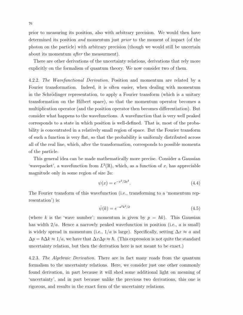
76

prior to measuring its position, also with arbitrary precision. We would then have

determined its position and momentum just prior to the moment of impact (of the

photon on the particle) with arbitrary precision (though we would still be uncertain

about its momentum after the measurment).

There are other derivations of the uncertainty relations, derivations that rely more

explicitly on the formalism of quantum theory. We now consider two of them.

4.2.2. The Wavefunctional Derivation. Position and momentum are related by a

Fourier transformation. Indeed, it is often easier, when dealing with momentum

in the Schrodinger representation, to apply a Fourier transform (which is a unitary

transformation on the Hilbert space), so that the momentum operator becomes a

multiplication operator (and the position operator then becomes differentiation). But

consider what happens to the wavefunctions. A wavefunction that is very well peaked

corresponds to a state in which position is well-defined. That is, most of the proba-

bility is concentrated in a relatively small region of space. But the Fourier transform

of such a function is very flat, so that the probability is uniformly distributed across

all of the real line, which, after the transformation, corresponds to possible momenta

of the particle.

This general idea can be made mathematically more precise. Consider a Gaussian

‘wavepacket’, a wavefunction from L2(R), which, as a function of x, has appreciable

magnitude only in some region of size 2a:

ψ(x) = e−x2/2a2

. (4.4)

The Fourier transform of this wavefunction (i.e., transforming to a ‘momentum rep-

resentation’) is:

ψ(k) = e−a2k2/2 (4.5)

(where k is the ‘wave number’; momentum is given by p = ~k). This Gaussian

has width 2/a. Hence a narrowly peaked wavefunction in position (i.e., a is small)

is widely spread in momentum (i.e., 1/a is large). Specifically, setting ∆x ≈ a and

∆p = ~∆k ≈ 1/a, we have that ∆x∆p ≈ ~. (This expression is not quite the standard

uncertainty relation, but then the derivation here is not meant to be exact.)

4.2.3. The Algebraic Derivation. There are in fact many roads from the quantum

formalism to the uncertainty relations. Here, we consider just one other commonly

found derivation, in part because it will shed some additional light on meaning of

‘uncertainty’, and in part because unlike the previous two derivations, this one is

rigorous, and results in the exact form of the uncertainty relations.

77

Given an observable, F , define ∆F := F − 〈F 〉. (The right-hand side is the

expectation value of F , where we have left the state unspecified.) The expectation of

(∆F )2 is the dispersion of F . Indeed,

〈(∆F )2〉 =⟨F 2 − 2F 〈F 〉+ 〈F 〉2

⟩= 〈F 2〉 − 〈F 〉2, (4.6)

which is a standard statistical notion of ‘dispersion’ (often called ‘mean-square de-

viation’ by physicists, and ‘variance’ by statisticians; its square root is the standard

deviation). Now, let F and G be observables (self-adjoint operators). Then the

Schwarz Inequality (§7.1.3) implies that

〈(∆F )2〉〈(∆G)2〉 ≥ |〈∆F∆G〉|2. (4.7)

Straightforward algebraic manipulations (see, e.g., Sakurai 1985, p. 36) transform

(4.7) into the standard uncertainty relation:

〈∆F 〉〈∆G〉 ≥ 1

2|〈[F,G]〉|. (4.8)

for any observables F and G. Notice, for example, that

〈∆P 〉〈∆Q〉 ≥ 1

2. (4.9)

(or, if we are not setting ~ = 1, then the right-hand side is ~/2—see note 11).

Above, we said that this derivation would shed some light on the meaning of un-

certainty. In particular, we can now see that, rigorously, ‘uncertainty’ refers to the

dispersion (standard deviation) of an observable in a given state, which is normally

understood as a measure of the ‘spread’ in its values over an ensemble of systems all

in some given state.

4.2.4. Limitations and Generalizations. The derivation of (4.8) makes it clear that

any two non-commuting operators will give rise to some uncertainty relation. Hence

(4.8) is quite general. However, there are also ‘uncertainty relations’ between quanti-

ties that are not represented by operators. The most well-known is the time-energy

uncertainty relation, whose interpretation is notoriously problematic precisely be-

cause time is not an observable in quantum theory. (There is no self-adjoint operator

that represents time.) Another example is phase and photon number. (Again, there

is no ‘phase’ operator.) Various proposals exist for how to understand these other

uncertainty relations, but here we merely note the point that they must apparently

be understood in some sense other than that given by (4.8).

Moreover, (4.8) faces other problems. First, recall that (4.8) is state-dependent.

Indeed, if we choose a state that is an eigenstate of F (or G), then even if F and G

do not commute, both sides of (4.8) are zero, which certainly seems to violate the

78

spirit of ‘uncertainty’. (The ‘solution’, perhaps, is to notice that if F and G do not

commute, then in general the dispersion of G for a system in an eigenstate of F will

be non-zero.) Second, keep in mind that ‘dispersion’ itself can be misleading. Even

when most of the probability is concentrated on a narrow range of possible values of

F , a small amount of probability that is located very far from F ’s mean can cause its

dispersion to become large. There are proposals to handle these shortcomings. (See

especially Uffink 1994.)

4.2.5. ‘Wave-Particle Duality’. A quantum-theoretic experiment that is commonly

associated with the uncertainty principle is the double-slit experiment (which had

been done, in some form, from well before the advent of quantum theory). The set-

up is as follows: a source of particles (or monochromatic light, i.e., photons) is placed

in front of an opaque barrier with two parallel slits. Behind the barrier is a screen

(such as a photographic plate). A particle is fired at the slits in the barrier, and the

screen records the location of each particle as it strikes the screen. (See figure 3.)

source barrier

screen

Figure 3. Double-Slit Experiment.

The main point is the following. We shine a beam of particles from the source onto

the barrier. If both slits are left open and no determination is made about which slit

the particle traverses, then an interference pattern develops on the screen, which is

just what one would expect if a wave somehow passes through the slits. (See figure

4a.) If, on the other hand, we determine which slit the particles traverse, then no

interference pattern shows up on the screen—instead, a pattern that is characteristic

of particles (one ‘blob’ behind each slit) shows up. (See figure 4b.) What is more, one

can do the experiment one particle at a time, and in this case, one sees ‘dots’ on the

screen, and yet, if no determination is made about which slit the particles traverse,

eventually the dots exhibit an interference pattern. (See figure 4c.)

This experiment illustrates ‘wave-particle duality’: when we measure a wave-like

property of particles (interference), we get wave-like behavior (interference pattern),

while when we measure a particle-like property of particles (which slit a particle

traverses), we get particle-like behavior (no interference pattern).

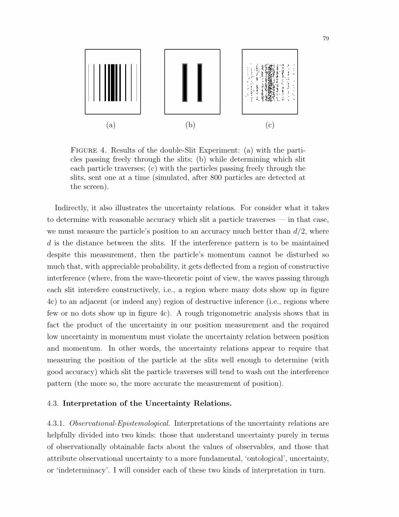
79

(a) (b) (c)

pppppppppppppppppppppppppppppppppppppppppp

ppppppppppppppppppppppppppppppppppppppppppppppppppppppppppppppppppppppppppp

ppppppppppppppppppppppppppppppp

ppppppppppppppppppppppp

pppppppppppppppppppppppppppppppp

pppppppppppp

ppppppppppppppppppppppppppppppppppppppppppp ppppppppppppppppppppppppppppppppppppppppppppp

ppp

ppppppppppppppppp

ppppppppppppppp

ppppppppppppppppppppppppppppppppppppppppppppppppppppppppppp

ppp p

ppppppppppppppppppppppppppppppppppppppppppppppppppppppppppppppppppppppppppppppppppppppppppppppppppp

ppppppppppppppppppppppppppppppppppppppppppppppppppppppppppppppppppppppp

pppp

pppppppppppppppppppppppppppppppppppppppppppppppppppppppppppppppppppppppppppp

ppppppppppppppppppppppppppppppppppppppppppppppppp

ppppppppppppppppppppppppppppppp

ppp

pppppppppppppppp

pppppppppppppppppppppppppppppp ppp

pppppppppppppppppppppppppppppp

ppppppp pp

pppp

p

ppp

pp

pp

pp p

pp p pp p

pp

ppp

ppp p

p ppp pppp p

pp

pp p pp

pp pp

p pp

ppp pp pp

pp

pp

p ppp

Figure 4. Results of the double-Slit Experiment: (a) with the parti-cles passing freely through the slits; (b) while determining which sliteach particle traverses; (c) with the particles passing freely through theslits, sent one at a time (simulated, after 800 particles are detected atthe screen).

Indirectly, it also illustrates the uncertainty relations. For consider what it takes

to determine with reasonable accuracy which slit a particle traverses — in that case,

we must measure the particle’s position to an accuracy much better than d/2, where

d is the distance between the slits. If the interference pattern is to be maintained

despite this measurement, then the particle’s momentum cannot be disturbed so

much that, with appreciable probability, it gets deflected from a region of constructive

interference (where, from the wave-theoretic point of view, the waves passing through

each slit interefere constructively, i.e., a region where many dots show up in figure

4c) to an adjacent (or indeed any) region of destructive inference (i.e., regions where

few or no dots show up in figure 4c). A rough trigonometric analysis shows that in

fact the product of the uncertainty in our position measurement and the required

low uncertainty in momentum must violate the uncertainty relation between position

and momentum. In other words, the uncertainty relations appear to require that

measuring the position of the particle at the slits well enough to determine (with

good accuracy) which slit the particle traverses will tend to wash out the interference

pattern (the more so, the more accurate the measurement of position).

4.3. Interpretation of the Uncertainty Relations.

4.3.1. Observational-Epistemological. Interpretations of the uncertainty relations are

helpfully divided into two kinds: those that understand uncertainty purely in terms

of observationally obtainable facts about the values of observables, and those that

attribute observational uncertainty to a more fundamental, ‘ontological’, uncertainty,

or ‘indeterminacy’. I will consider each of these two kinds of interpretation in turn.

80

4.3.1.1. Uncertainty as Uncertainty. The term ‘uncertainty’, and the understanding

of uncertainty as standard deviation (dispersion), strongly suggests an epistemic,

even operationalist, understanding of the uncertainty relations. In particular, one is

quite tempted to understand the uncertainty relations in terms of post-observational

uncertainty about the actual values of observables.

There is a question about whether this uncertainty concerns single systems, or en-

sembles. In the latter case—i.e., if, as suggested by the usual statistical understanding

of standard deviation, we understand uncertainty to reflect dispersion of values (for

some observable) in an ensemble—the ‘interpretation’ of the uncertainty relations

does not go beyond a straightforward statistical understanding of standard deviation.

Of course, in this case then there is still a sense in which uncertainty applies to sin-

gle systems, namely, when they drawn at random from such an ensemble. But one

might, in addition, suppose that the notion of uncertainty applies to single systems

independently of the consideration of any ensemble. Indeed, one might argue that

only in this case would we really , understand why uncertainty holds at the statistical

level. In any case, let us consider that possibility.

The idea, then, is that measurement (more generally, observation) in general re-

duces our uncertainty about the value of some observable, F , on the (single!) mea-

sured system. The uncertainty principle would then be read as asserting that a

reduction in uncertainty about the value of F can imply an increase in uncertainty

about the values of observables that are incompatible with F .

The meaning of such an assertion is clear enough, but understanding why incom-

patible observables have this feature is another matter. Suppose that F and G are

incompatible. Suppose that we measure F . We then measure G. Why should it be

the case that this second measurement ruins our previous knowledge of the value of

F? Indeed, supposing that the second measurement is isolated from the first, and

that the value of F was not in any way disturbed in the meantime, how could the

second measurement ruin our previous knowledge of the value of F?

4.3.1.2. Einstein’s Early Thought Experiment. Early critics of quantum theory—notably,

Einstein—asked something like this question, and indeed proposed (thought) experi-

ments that were apparently intended to show that in fact it is possible to ‘beat’ the

uncertainty principle. A famous such experiment, due to Einstein, involves a standard

two-slit apparatus (see figure 3) that is mounted on springs. The basic idea is to use

the springs to determine which slit the particle traversed, without in fact disturbing

the particle itself, by measuring the exchange of momentum between the particle and

the barrier. (If the source is located on the plane exactly between the slits, then if

81

the particle goes through the right-hand slit (and the slits are narrow enough), the

barrier will in general experience a kick to the right, and so on.)

4.3.1.3. Reply to Einstein. Einstein’s challenge to the uncertainty principle, here, is

empirical: he is claiming that, contrary to what quantum theory allows, it is possible

to prepare a system in a state of precise position and momentum (or at any rate,

more precise than the uncertainty relations allow). The response must, therefore, be

empirical. If indeed it is possible to prepare a system in a precise state of position

and momentum, then we ought to be able to use our knowledge of either to make

a verifiable prediction about the system. In particular, if the measurement of the

position of the particle right after it passes through the slits does not, in fact, disturb

the momentum of the particle, then we should still see the same interference pattern

on the screen that we see in the standard two-slit experiment. If, on the other hand,

the interference pattern ‘washes out’ (see §4.2.5), and approaches the ‘two blobs’ (see

figure 4b) as the measurement of position becomes more and more precise, then the

epistemic version of the uncertainty principle stands.

As far as current experiment can discern, it seems that a measurement of which

slit the particle traverses does indeed wash out the interference pattern. Indeed, a

remarkable experiment appears to show that not even this much is quite right; rather,

what seems to matter is whether a record of the result of the measurement is kept,

where by a ‘record’, here, we mean an encoding of the result in a measurable physical

state of the universe. The experiment59 is, in essence, the two slit experiment, with

a detector placed behind one of the slits. The detector is, moreover, ‘eraseable’, in

the following sense. Once a particle passes through the detector, the particle leaves

a trace in the state of the detector. We may then choose to magnify this ‘trace’ in

order to turn it into a discernible signal indicating the presence of the particle, or

we may completely erase it, so that the state of the detector no longer contains any

retrievable information about whether the particle was once in the detector.

With this erasable detector in place, now imagine performing the following experi-

ment. Fire the particles at the barrier one at a time. After the particle passes through

the barrier, either erase the detector, or not. On the runs where we erase the detector,

the particles build up an interference pattern (as in figure 4c). On the runs where we

do not erase the detector, the particles do not build up an interference pattern, but

instead ‘behave as particles’ (as in figure 4b). The experiment is relatively recent, and

requires further scrutiny, but it strongly suggests, as do other quantum-mechanical

experiments, that the epistemic version of the uncertainty principle is a fact of nature.

59See, for example, Scully and Walther (1989) and Walborn et al. (2002).

82

4.3.2. Ontological. With the epistemic version of the uncertainty principle apparently

intact, we are left wondering why it is true. Different interpretations will propose

different answers to this question. Some assert a ‘disturbance theory’, according to

which the measurement of one quantity physically disturbs others (corresponding to

incompatible observables) in an uncontrollable and unpredictable way. Others assert

that reality matches our knowledge, here: we cannot know the value of G (when the

value of incompatible F is known) because, in fact, G has no value.

There are many versions of this idea. Here we consider two. The first, often

claimed to be part of the ‘Copenhagen’ interpretation of quantum theory, rests on

some version of a verificationist, or operationalist, theory of the meanings of physical

quantities, according to which a physical quantity has a value if and only if it has been

measured (i.e., verified—the appropriate physical operations have been carried out,

with the appropriate outcome). One must then argue that it is physically impossible

to perform measurements of incompatible observables simultaneously on the same

system.

This argument suggests a second ontological version of the uncertainty principle,

according to which a physical quantity is well-defined just in case the conditions

required for its well-definedness obtain. Of course, stated thus, this view sounds

almost tautologous. It’s real content comes from arguing that there are indeed non-

trivial physical conditions that must be in place in order for certain physical quantities

to be well-defined, and that the conditions required for the well-definedness of a given

quantity cannot be in place simultaneously with the conditions required for the well-

definedness of any incompatible quantity.

This sort of argument has bite, if it does, because of the role of reference frames

in the definition of physical quantities (§3.4). Hence, for example, ‘momentum’ must

mean ‘momentum relative to X’, where ‘X’ is some physical system that defines a

frame of reference. But if ‘X’ (more precisely, the frame of reference that it defines)

is a non-inertial system, then it is not suitable for defining momentum (at least not

over any stretch of time), unless we know its relation to some inertial frame F (but

then we are really defining momentum relative to F )—recall §3.4.1. Similarly, a non-

inertial physical system is inappropriate for defining position (with the same caveat

as before). These brief points recall the more extensive discussion above, and we shall

have to leave the matter at that.

4.4. The Einstein-Podolsky-Rosen Argument. Thus far, everything that has

been said about the uncertainty relations is consistent with the claim that the loss of

certainty about the value of one observable, F , upon measurement of incompatible G,

83

is a result of an unknown and uncontrollable physical disturbance of the value of F as

a consequence of the measurement of G. Indeed, Heisenberg’s ‘optical’ derivation of

the uncertainty relations uses precisely this idea. But an argument due to Einstein,

Podolsky, and Rosen (EPR)60 purports to show that in fact the uncertainty relations

cannot be understood in this way.

This argument concedes that the epistemic version of the uncertainty principle is

true: the values of incompatible observables are not simultaneously verifiable. The

point, here, is to question ontological versions of the principle.

4.4.1. Incompleteness. In particular, the point is to call into question the complete-

ness of quantum theory. Recall (§1.2.3.9) the standard interpretation of quantum

theory, according to which an observable, F , has a value for a system in a state,

W , just in case W assigns probability 1 to some possible value of F (and 0 to the

others). This interpretation immediately implies that there are no quantum states

that assign simultaneously definite values to all observables, or indeed to any two ob-

servables with no common eigenvectors. Hence any argument that successfully shows

that two such observables must have definite values implies that quantum theory is

incomplete—more precisely, it shows that under the standard interpretation of the

theory, quantum states do not describe (and cannot describe) the complete physical

state of a system. The EPR argument purports to show exactly this claim.

4.4.2. The Generic Experiment. Generically, the experiment considered by EPR in-

volves a pair of particles (call them α and β) prepared in the state

|ΨEPR〉 =1√N

N∑n=1

|an〉|bn〉 (4.10)

where the |an〉 and the |bn〉 form orthonormal sets.61 Hence there are observables, A

for system α and B for system β (whose eigenvectors are respectively the |an〉 and the

|bn〉, corresponding to eigenvalues an and bn) that are perfectly correlated (§1.2.6.4)

in this state.

So suppose that α and β are in the state |ΨEPR〉 while they are spatially separated.

Then the perfect correlation between A and B allows one to discover the value of A

without, as EPR say, ‘in any way disturbing’ α, simply by measuring B on β.

60There are very good reasons to believe that the argument as presented by EPR (1935) was notquite what Einstein himself had intended. (The paper was not written by him.) See Fine (1986,esp. chs. 3-5, for example.

61In fact, there is a ‘continuous’ version of (4.10), which is appropriate when we are consideringobservables, such as position and momentum, with continuous spectra. See §4.4.3.

84

Now for the crucial point. Consider orthonormal bases {|a′n〉} and {|b′n〉} obtained

from the |an〉 and the |bn〉 as follows:

|a′n〉 =1√2

(|an〉 − i|an+1〉

)|b′n〉 =

1√2

(|bn〉+ i|bn+1〉

), (4.11)

where the sum in subscripted ’n+ 1’ is modulo-N (i.e., N + 1 = 1). In this basis, the

state |ΨEPR〉 has exactly the same form:

|ΨEPR〉 =1√N

N∑n=1

|a′n〉|b′n〉. (4.12)

(To verify, plug (4.11) into (4.12) and simplify. The ‘cross’ terms of the form−i|an〉|bn+1〉and i|an〉|bn+1〉 cancel.) Hence there are additional observables, A′ and B′ (whose

eigenvectors are respectively the |a′n〉 and the |b′n〉) that are also perfectly correlated

in the state |ΨEPR〉. Moreover, A′ does not commute with (is incompatible with)

A—indeed, they share no eigenvetors—and similarly for B and B′. Again, we can

discover the value of A′ on α by measuring B′ on β.62

Finally, notice that this entire description is quantum-mechanical. One sometimes

hears the EPR experiment described in more or less classical terms. For example,

letting A and B be position and momentum (see §4.4.3), one might be tempted to

describe the preparation of the EPR state as follows: fire two particles of equal mass

from a common source with equal (in magnitude) but oppositely directed forces.

Their positions (distance from the source) and momenta (relative to the source) will

then be perfectly correlated. This picture is tempting, but it is also completely wrong.

Indeed, standard quantum mechanics implies that the state just described cannot be

prepared in a way that would allow one to infer the position (or momentum) of α

from that of β, because such inferences would require us to know, with precision,

the position and momentum of the source, and such knowledge already violates the

(epistemic) uncertainty principle.

4.4.3. Position and Momentum. Above we assumed that the perfectly correlated ob-

servables have a discrete spectrum. In fact, when they consider an explicit example

(rather than the abstract case as considered above), EPR refer to position and mo-

mentum, and a state that is perfectly correlated in position and momentum (in the

sense that it is a simultaneous eigenstate of the sum of the momenta of the two

particles, and the difference of their positions). Explicitly,

ΨEPR(x1, x2) =

∫ +∞

−∞e(2πi/h)(x1−x2+x0)pdp, (4.13)

62The situation as described here is not mathematically exactly the same as that considered byEPR, but the result is the same.

85

for some fixed x0. However, it is worth pointing out that in fact this state is not an

allowed state of the system at all—it is not a vector in L2(R2). Moreover, this state,

even if it could be prepared, necessarily spreads under any time evolution (associated

with a finite potential energy), hence immediately becoming a state of less than

perfect correlation.63

To overcome these limitations of EPR’s example, one could consider, for example,

a narrow Gaussian that is very close to being a state of perfect correlation, but doing

so makes the argument to come messy at best. And we should keep in mind that the

discussion in terms of position and momentum is in fact only an example that EPR

give to illustrate the main point.

In the end, in fact, it is easier to consider an example that involves bounded observ-

ables. The simplest case is the so-called ‘singlet’ state of a pair of spin-1/2 particles.

Generically, this case corresponds (for an appropriate choice of the |an〉 and the |bn〉)to the state |ΨEPR〉 above, for N = 2. We will just continue to speak of the observ-

ables A, A′, B, and B′, with the understanding that the perfect correlations discussed

above obtain.

4.4.4. The Argument. How can this experimental situation be used to generate an

argument for the incompleteness of quantum theory? The conclusion that EPR hope

to establish is that A and A′ both have a definite value simultaneously. Because

they share no common eigenvectors, this conclusion is inconsistent with the standard

interpretation of quantum states (see §1.2.3.9).

One tempting path to this conclusion involves presuming that once B has been

measured on β, thereby establishing the value of A on α, we can measure A′ on α

and thereby establish its value directly. However, the problem with this suggestion

should be clear: the disturbance theory of uncertainty can quickly be applied to

conclude that the measurement of A′ on α disturbs the previously established value

of A. We are thus reminded that the point of this discussion is, in fact, to establish

the definiteness of A and A′ without ‘in any way’ disturbing α.

EPR’s strategy involves two assumptions. The first, with which at least some

versions of the standard interpretation can easily agree, is their ‘criterion for physical

reality’, which asserts that whenever the value of an observable can be predicted

with certainty, the observable actually has that value. (Notice that this criterion is

inconsistent with the sort of verificationist or operationalist views, mentioned above

(§4.3.2), according to which a system has a value only if that value has been obtained

63By the state ‘spreading’, here, we mean, roughly, that it gets closer to a uniform distributionover R2. See Dickson (2002b) for a discussion of these points, and further references.

86

as the result of a measurement.) Before we introduce the second assumption, let us

see how far we can get with just this one.

Notice that if we measure B on β, we can predict the value of A on α with certainty.

Similarly for B′ and A′. Of course, we cannot measure both B and B′. Hence, instead

of considering actual measurements of B and B′, let us consider non-actual, but

possible (i.e., ‘counterfactual’) measurements of B and B′. We have:

Premise 1: Possibly, B is measured on β, and in this case, α has a definite

value for A.

Premise 2: Possibly, B′ is measured on β, and in this case, α has a definite

value for A′.

From these two premises (which follow from the criterion for physical reality), EPR

hope to conclude:

Conclusion: Possibly, α has a definite value for both A and A′.

However, the Conclusion does not follow from the Premises 1 and 2. Indeed, the

logical problem is, in part, that there is no guarantee that the possible conditions

(‘B is measured’ and ‘B′ is measured’) are co-possible. Indeed, as we know, they are

not.64

Hence EPR need another premise. They introduce a notion of ‘non-disturbance’

that is supposed to help patch up the argument: although the conditions (measure-

ment of B) under which we can infer the definiteness of A on α are incompatible with

the conditions (measurement of B′) under which we can infer the definiteness of A′,

the difference between them is supposed to make no difference to α, because they

only involve a change of circumstances for β, which may be spatially separated from

α.

However, not just any such principle will work. Consider, for example, the follow-

ing:

Weak non-disturbance: if B is measured on β and (therefore, by the criterion

for physical reality) A is definite for α, then: had we not measured B on β, α

would still have had a definite value for A (and likewise, substituting primed

observables for the unprimed ones).

64Consider the following analogous argument. (i) It is possible that the paper is burned, and inthis case it will be reduced to ashes. (ii) It is possible that the paper is not burned, and in thiscase it will remain whole. Therefore, (iii) it is possible that the paper is both whole and reduced toashes. Of course, this argument is invalid.

87

This principle, which might be taken to deny that measuring B is what brings it

about that A has a definite value, is insufficient to get EPR’s conclusion. They need,

instead:

Strong non-disturbance: if B is measured on β and (therefore, by the crite-

rion for physical reality) A is definite for α, then: had we instead measured B′

on β, α would still have had a definite value for A (and likewise, substituting

primed observables for the unprimed ones).

The weak principle is insufficient to get the conclusion because the introduction of the

measurement of B′ (as opposed to the mere absence of the measurement of B) could

destroy essential features of the situation, and in particular features that permit the

inference of properties of α (its value for A) from the results of measurements (of B)

on β.65

The principle of strong non-disturbance is supposed, of course, to capture some

notion of ‘locality’. In particular, the idea is supposed to be that nothing that is

done to β can have any affect on the properties of α, under the assumption that

the two particles are space-like separated. Einstein’s theory of special relativity is

presumably supposed to license this asusmption.66 In any case, with the principle

of strong non-disturbance, EPR have a logically valid argument for the Conclusion,

above. Indeed, they could (and seem to claim to) establish a stronger form of the

conclusion, replacing ‘Possibly’ with ‘Actually’, as follows. Argue, further, that a

measurement of B (or B′) does not bring it about that α has a value for A (A′), so

that α must have values for both A and A′ even when B (B′) is not measured.

4.4.5. Replies to EPR. One can, in fact, deny strong non-disturbance by denying

locality. We shall consider the status of locality in quantum theory below (§6). Here,

we consider two other replies to EPR.

We have already more or less encountered one of these replies: note that the EPR

argument has no impact on those verificationist or operationalist views according

to which an explicit measurement of a physical quantity is required not merely for

us to know its value, but also for it to have a value. Of course, such views must

deny the criterion for physical reality (which, keep in mind, is only a sufficient, not

a necessary condition), and many find this principle quite compelling. (Apart from

65The possible-worlds semantics for counterfactuals makes the point easy to see: while the closest‘B is not measured’-worlds to the ‘B is measured and A is definite for α’-worlds might all be ‘A isdefinite for α’-worlds, those closest worlds might not contain any ‘B′ is measured’-worlds, so thatthe closest ‘B is not measured but B′ is’-worlds to the ‘B is measured and A is definite for α’-worldsneed not be ‘A is definite for α’-worlds.

66See Malament, Ch. 3, this volume.

88

actually having the value in question, what else could, reasonably, make it be the

case that we can predict its value with certainty?)

But Bohr offered a reply that appears to rely neither on this verificationist or

operationalist strategy, nor—so he claims—on an explicit endorsement of non-locality.

In particular, recall that EPR were aiming to avoid the ‘disturbance’ account of

uncertainty, according to which, for example, a measurement of A′ physically disturbs

the value of A. Here, because we are only ever performing measurements on β, it is

far from clear how a measurement of B′, for example, could disturb the value of A

on α—after all, such a disturbance would have to be non-local. Bohr’s reply denies

strong non-disturbance, but without (so the claim goes) endorsing a physically direct

(Bohr uses the term ‘mechanical’) disturbance of (e.g., the value of A for) α as a

consequence of any measurement (e.g., of B) on β. Instead, recall the idea from

above (§4.3.2), that the very well-definedness of certain physical quantities relies on

certain physical conditions being in place.

Indeed, consider the EPR experiment, now, as Bohr (and EPR) did, in terms of po-

sition and momentum. We will assume (without loss of generality) that the positions

and momenta are defined relative to the source. On Bohr’s view, the well-definedness

of the sum of the momenta for each particle (i.e., the total momentum for the system)

is maintained just so long as the system (particles plus source) remains closed, i.e.,

just as long as total momentum is conserved. But a measurement of the position

of β introduces a disturbance of β’s momentum. The system is no longer closed: β

either loses momentum to or gains momentum from an object (the measuring appa-

ratus) that is external to the system. But then the total momentum (relative to the

source, which ‘knows nothing’ about this external influence on β) is no longer con-

served, and thus the conditions for its well-definedness (relative to the source) are no

longer in place, and therefore any inferences that we might have made about the well-

definedness of α’s momentum, based on the well-definedness of the total momentum,

are no longer valid. In other words, on Bohr’s view, the conditions required (under

the circumstances) for the well-definedness of α’s momentum are, when we are mea-

suring β’s position, no longer in place. Note that the ‘old’ type of disturbance is still

at work here—we are indeed supposing that β’s momentum is physically disturbed by

a measurement of its position—but in addition there is another type of disturbance

at work: the measurement of β’s position ‘disturbs’ the conditions required for the

well-definedness of α’s momentum (under the circumstances). Thus Bohr believes

that he can avoid EPR’s conclusion by (in essence) denying strong non-disturbance,

89

but in a way that does not entail a non-local disturbance, in the sense of an exchange

of energy or momentum between β and α.

4.4.6. Where We Stand. Regardless, finally, of whether one finds any of these replies

to EPR satisfactory (and we should not make any judgment on this point at least

until we have considered the issues in §5 and §6, it should be emphasized that none

of them shows that the EPR argument is unsound, much less invalid. Indeed, they

are, in a sense, defensive maneuvers designed to articulate a view of quantum theory

that avoids EPR’s conclusion by denying, in a consistent and presumably plausible

way, one of the premises of their argument. Their conclusion is thus far from called

into question by such replies. Indeed, many philosophers of quantum theory are more

or less in agreement with EPR that standard quantum theory is incomplete, if not

because of EPR’s argument, then because of the so-called ‘measurement problem’,

which we consider next.

5. The ‘Measurement Problem’

The problem of measurement is, perhaps, the most discussed issue in the foun-

dations of quantum theory, and has inspired numerous and varied interpretations of

the theory, from the brilliant to the bizarre. In this section, I will first review the

problem (§5.1), emphasizing its generality. Then I will consider some natural, but in

the end unsatisfactory, reactions to the problem (§5.4). In the final section (§5.5),

I will consider a few examples of interpretations of the theory, each of them largely

directed towards solving the measurement problem.

5.1. The Basic Problem.

5.1.1. ‘Schrodinger’s Cat’. Recall (1.2.3.2.b) that the superposition principle implies

that for any observable, F , if a system can have each (or indeed, just two of) the

eigenvalues of F as its values for F , then it is also possible for a system to have

(assuming the eigenstate-eigenvalue link, §1.2.3.9) no value for F (because it is in a

superposition of the eigenstates of F ).

If F is some unfamiliar observable of the unfamiliar quantum world, then perhaps

one can live with this consequence. But what about observables on middle-sized solid

objects that are the bread and butter of our everyday experience? What about ‘the

(approximate) location of the house’, or ‘the (approximate) momentum of the horse’,

and so on? In 1935, Schrodinger illustrated the sort of problem that we face with the

following example.

90

One can even set up quite ridiculous cases. A cat is penned up in a

steel chamber, along with the following device (which must be secured

against direct interference by the cat): in a Geiger counter there is a

tiny bit of radioactive substance, so small, that perhaps in the course

of the hour one of the atoms decays, but also, with equal probability,

perhaps none; if it happens, the counter tube discharges and through

a relay releases a hammer which shatters a small flask of hydrocyanic

acid. If one has left this entire system to itself for an hour, one would

say that the cat still lives if meanwhile no atom has decayed. The

psi-function of the entire system would express this by having in it the

living and dead cat (pardon the expression) mixed or smeared out in

equal parts. (Schrodinger 1935a)

The point, of course, is that after some stretch of time, the atom is in a superposition

of ‘decayed’ and ‘not decayed’, and hence the hammer, poison, and ultimately the

cat, are in corresponding superpositions—in the case of the cat, a superposition of

‘alive’ and ‘dead’. But of course we never witness cats in such states. So apparently

there is a serious problem with quantum theory.

5.2. Measurement. Notice that the cat serves, in essence, as a decay-indication

device, a kind of crude measuring apparatus. Indeed, it is precisely Schrodinger’s

point that one can magnify a superposition at the microscopic level (the atom) to

a superposition at the macroscopic level (the cat), the level at which one is proba-

bly more inclined to deny categorically that superpositions (of at least some sorts,

such as of the states ‘alive’ and ‘dead’) make any sense, physically, or at any rate

that they exist with anything like the frequency that quantum theory apparently pre-

dicts. Measurement devices designed to measure quantum-mechanical observables are

characteristically of this sort: they ‘magnify’ the state of some microscopic quantum

system into the (indicator, or ‘pointer’) state of an apparatus that can be directly

observed.67

Of course, this magnification is a physical process, and as such, it is in principle

to be described as a solution to Schrodinger’s equation (or some other quantum-

theoretic equation of motion). Those equations are linear. (In fact, it is precisely this

linearity that partially grounds the principle of superposition: any linear combination

67Recall my earlier (§1.4.3) skepticism, however, about ‘pure’ states such as |cat dead〉. Does thisskepticism suggest a way out of the measurement problem? Alas, it does not. We could just as wellspeak in terms of mixed states, here, and generate the problem, which relies only on the fact thatat the end of a measurement, the state of the apparatus may assign non-trivial probabilities to allpossible values of the ‘pointer-observable’.

91

of solutions is again a solution.) Indeed, recall that the dynamical evolution of a

system can be described in terms of a family of unitary operators, which are, of

course, linear.

So let a given measurement-interaction (between some apparatus and some mea-

sured system) be described by the operator U . (As an example, recall §3.1.2.) Let

the apparatus’ ‘ready-to-measure’ state be |Ψ0〉 and let its ‘pointer’ states be |Ψn〉.For each of the eigenstates, |fn〉 of the measured observable, F , we presume that the

measurement-interaction results in an accurate indication of the result:

U(|fn〉|Ψ0〉) = |fn〉|Ψn〉 (5.1)

so that the state |Ψn〉 indicates that the measured system has the value fn for F . But

then, by linearity,

U

(∑n

kn|fn〉|Ψ0〉

)=∑

n

kn|fn〉|Ψn〉. (5.2)

Now we are in trouble. The eigenstate-eigenvalue link implies that this final state

is one in which the pointer-observable for the apparatus in fact has no value. The

pointer is not indicating anything. But at the end of typical successful measure-

ments, the apparatus does indicate a result, even when the measured system begins

in a superposition of eigenstates of the measured observable. Standard quantum the-

ory seems to contradict this apparent fact of experience. Hence the ‘measurement

problem’.

5.3. Generality of the Problem. There are at least three senses in which the

‘measurement problem’ as described above does not capture the real problem with

sufficient generality. First, it relies on the quite conservative eigenstate-eigenvalue

link, and on a very restrictive notion of ‘measurement’. Second, it fails to indicate

the ubiquity of superpositions. Third, it relies on the questionable assumption that

the macroscopic pointer-states of the apparatus are pure states, when in fact they are

almost surely mixed. In this subsection I will briefly consider these points. Finally, I

will briefly raise a related problem, the problem of the ‘classical limit’.

5.3.1. ‘No-go’ Theorems. Two important premises in the argument leading up to the

measurement problem, above, were the eigenstate-eigenvalue link and the account

of what counts as a successful ‘measurement’. Both of these assumptions can be

weakened considerably.68 I will consider each in turn.

68There is a long history of proofs, increasingly general, that the measurement problem is ‘in-soluble’ in the context of standard quantum theory. A review of the early history, together witharguably the simplest proof of the theorem, is given by Brown (1986). For a more recent survey andextensive discussion of this issue, see Mittestaedt (1998, esp. ch. 4).

92

5.3.1.1. Weaker Conditions for Definiteness. First, we may introduce a weak condi-

tion for when an observable has a definite value, roughly as follows: the final state of

the apparatus assigns a definite value to the pointer-observable for the apparatus just

in case the final state of the compound system is a mixture of states each of which has

a definite value for the pointer observable according to the eigenstate-eigenvalue link.

In other words, we now allow the adoption of an ignorance interpretation of mixed

states of the compound system, accepting that when the compound system has the

sort of mixed state just described, it is actually in one of the pure states appearing in

the mixture, and therefore, according to the eigenstate-eigenvalue link, the apparatus

has a definite value for the pointer-observable.

Note that the condition applies to the compound system, not to the apparatus on its

own. The difference is subtle, but crucial. For example, in an ideal measurement, the

apparatus by itself will always be in a mixture of eigenstates of the pointer-observable.

It does not follow, however, that this mixture can be given an ignorance interpretation.

I shall discuss this point in a somewhat different context below (§5.4.5.2.a).

5.3.1.2. Weaker Accounts of Measurement. We may also weaken the account of mea-

surement, along the following lines. Let U represent the time-evolution of states of the

compound system during the measurement of a POVM, E, by a ‘pointer-observable’

POVM, Q. We require: for any two states, W and W ′, of the compound system, if

W and W ′ differ in their probabilities for at least one of the effects in the image of E,

then UWU−1 and UW ′U−1 differ in their probabilities for at least one of the effects

in the image of Q. Intuitively, U renders the pointer-observable ‘somehow sensitive

(even if only probabilistically) to the measured observable’.

Note, however, that while this weaker account of measurement, together with the

weaker criterion for definiteness (§5.3.1.1), is sufficient to derive the measurement

problem (i.e., the non-definiteness of the pointer-observable at the end of a measure-

ment), it is also worth keeping in mind that, by the bi-orthogonal decomposition

theorem (§1.2.6.2), there are some observables (one for the measured system and one

for the apparatus) with respect to which the state of the compound system has the

same form that it does in an ideal measurement. (I.e., write the state in its biorthogo-

nal form. The bases for the measured system and apparatus will be bases determined

by some observable for each.) On the other hand, whether this apparatus-observable

is one that we antecedently believe to be definite is another question, the answer to

which probably depends on the details of the interaction.

93

5.3.2. The Ubiquity of Superposition. The superposition principle asserts that super-

positions of possible states are again possible states. But perhaps they are extremely

rare. In that case, again perhaps we should not be terribly concerned about the

measurement problem.

In fact, however, superpositions at the microscopic level are ubiquitous. To see why,

we need only consider the case of spin. Recall that S~u and S~u′ are incompatible unless

~u = ~u′ or ~u = −~u′. Hence every spin-1/2 particle is ‘in a superposition’ with respect

to just about every direction of spin. A similar remark holds for the polarization of

photons. And there is good experimental and theoretical reason to believe that many

fundamental particles may have wavefunctions that are highly de-localized.

Moreover, we need not imagine exotic situations such as that described by Schrodinger

in order to believe that these microscopic superpositions may be ‘magnified’. While

such magnification is an important part of measurement, there is little reason to sup-

pose that it does not occur naturally, and frequently. After all, the human eye, for

example, is sensitive to as few as a half-dozen or so photons. It seems plausible to sup-

pose that many other interactions that occur in nature have the effect of correlating

the state of some macroscopic object with the state of some microscopic object—and

such correlation (even if imperfect) is sufficient for the sort of magnification that will

give rise to the measurement problem.

Hence, there is good reason to believe that the measurement problem is highly

general, in a few senses: (a) even under apparently weak accounts of when apparatus’

have a definite value for some macroscopic observable (§5.3.1.1), quantum theory

apparently implies that they do not; (b) the sort of correlation between a macroscopic

and microscopic object that is required in order to bring about the situation in (a) is

very weak, and moreover perfect correlations are, by the biorthogonal decomposition

theorem, ubiquitous (§5.3.1.2); and (c) the sort of superposition, and interaction, that

is required give rise to the situation in (b) is plausibly quite common (this section).

5.3.3. The Classical Limit. Finally, I will quickly notice a problem that is discussed in

detail elsewhere in this volume. In a sense, the measurement problem is the problem

that the ‘weirdness’ of the quantum world is somehow not confined to the microscopic

world. In other words, the ‘weird’ quantum world does not (always) mesh nicely with

our more familiar classical world, in the sense that superpositions at the micro-level

(where we might be able to live with them) are not confined to that level, but can be

made to appear at the macro-level (where, so the argument goes, we cannot live with

them). This apparent conflict leads to a more general question: how does quantum

theory go over to classical theory (which, after all, works quite well for a large domain

94

of objects in a wide variety of conditions)? The question is vexed in a number of ways,

which, however, we shall not consider here. We refer the reader to Landsman, Ch. 5,

this volume (esp. §§5,6).

5.4. Non-Solutions. Numerous solutions to the measurement problem have been

proposed, and we shall consider some of them in a separate section on interpretations.

Here, we consider several proposed solutions that in fact do not work, or at the very

least, face extraordinary obstacles to making them work.

5.4.1. Naıve Realism.

5.4.1.1. The Obvious Solution to the Rescue? The obvious solution to the problem is

to give up the eigenstate-eigenvalue link. Indeed, why not interpret the probabilities

delivered by quantum theory as entirely epistemic? That is, why not suppose that

every observable has a definite value all of the time, and that incompatibility merely

represents the fact that observing the value of one of them disturbs the values of others

in an incontrollable way? Something like an epistemic version of Bohr’s approach to

uncertainty, if it works, could be put to use in the service of this view, both accounting

for the uncertainty relations, and avoiding the measurement problem.

5.4.1.2. The Kochen-Specker Theorem. Initially attractive, this view founders on a

well-known theorem, the Kochen-Specker theorem (Kochen and Specker 1967). Notice

that naıve realism seeks to identify a single value for each observable. With one further

requirement, one can show that no such assignment is possible.

5.4.1.2.a. Non-Contextuality. This further requirement is specifiable in a variety of

ways. Here we put it in terms of ‘non-contextuality’. Note that assigning a value

to an observable amounts to assigning, to each set of mutually orthogonal subspaces

that span the entire space, a ‘1’ to exactly one of the subspaces, and ‘0’ to the others.

(These subspaces are the eigenspaces of the observable to which a value is assigned;

assigning a 1 to a given eigensubspace is equivalent to assigning the corresponding

eigenvalue to the observable.69 ) Proceeding in this way, we will further assume

that all observables with exactly the same eigenspaces have ‘the same’ value, in the

sense that they have the eigenvalue associated with a given common eigenspace. This

69Here I ignore observables, such as position and momentum, whose spectrum is continuous (sothat their possible values do not correspond to subspaces). After all, assigning them values as wellonly makes the naıve realist’s life even harder.

95

assumption amounts to the requirement that for any observable G, if G has the value

g, then for any function, f(), the observable f(G) has the value f(g).70

Non-contextuality includes this assumption, but goes a step further, requiring, in

addition, that the assignment of a ‘0’ or ‘1’ to a given subspace P is independent

of which set of mutually orthogonal and jointly spanning subspaces P is considered

to be a member. This requirement amounts to the condition that whenever two

observables, F and G, share an eigenspace, P (but do not necessarily share all of

their eigenspaces), F has the eigenvalue corresponding to P if and only if G does.

(The eigenvalues will in general differ, of course.) (Note that in this case F and G in

general will not commute.)

5.4.1.2.b. The State-Independent Theorem. Given non-contextuality, naıve realism

amounts to the requirement that we be able to find a homomorphism from the lattice,

L(H), of subspaces of a Hilbert space, H, to the Boolean lattice {0, 1}. That is, we re-

quire a map, h : L(H → {0, 1} such that, for any P,Q ∈ L(H, h(P ) ≤ h(Q) if and only

if P ≤ Q. It follows (from the definitions of the meet, joint, and orthocomplement,

which are all given in terms of the partial order—§7.4.2), that h(P )∧h(Q) = h(P∧Q),

h(P ) ∨ h(Q) = h(P ∨Q), and h(P )⊥ = h(P⊥). But notice that in {0, 1}, the opera-

tors ∧, ∨, and ⊥ behave just as those from classical logic (i.e.: 0 ∧ 0 = 0, 0 ∧ 1 = 0,

1∧1 = 1, 0∨0 = 0, 0∨1 = 1, 1∨1 = 1, and 0⊥ = 1). In other words, the naıve realist

requires that it be possible to consider quantum theory to arise from an underlying

(logically) ‘classical’ theory.

Such a picture is available in classical mechanics. Indeed, let Γ be the phase space

for a classical system. The physical propositions (cf. §2.1.1) are represented by the

lattice of Borel subsets of Γ (where the partial order is given by subset inclusion), and

it is possible to define a homomorphism from this algebra to {0, 1}. Indeed, choose

a point x ∈ Γ, and define the map, δx, by, for any Borel subset S ⊆ Γ, δx(S) = 1 if

x ∈ S and 0 otherwise. This δx is a homomorphism.

The content of the Kochen-Specker theorem is that for lattices of subspaces of a

Hilbert space whose dimension is greater than 2, there are no such homomorphisms.

This version of the theorem is sometimes called ‘state-independent’ because it does

not rely on any presumptions about the quantum state of a system, but only on the

structure of the state space as a whole.

5.4.1.2.c. State-Dependent Theorems. There are others versions of the theorem that

begin with the assumption that the system is in some given quantum state. In this

70Note that, in general, if G =∑

n gnPn is the spectral decomposition of G, then f(G) =∑n f(gn)Pn.

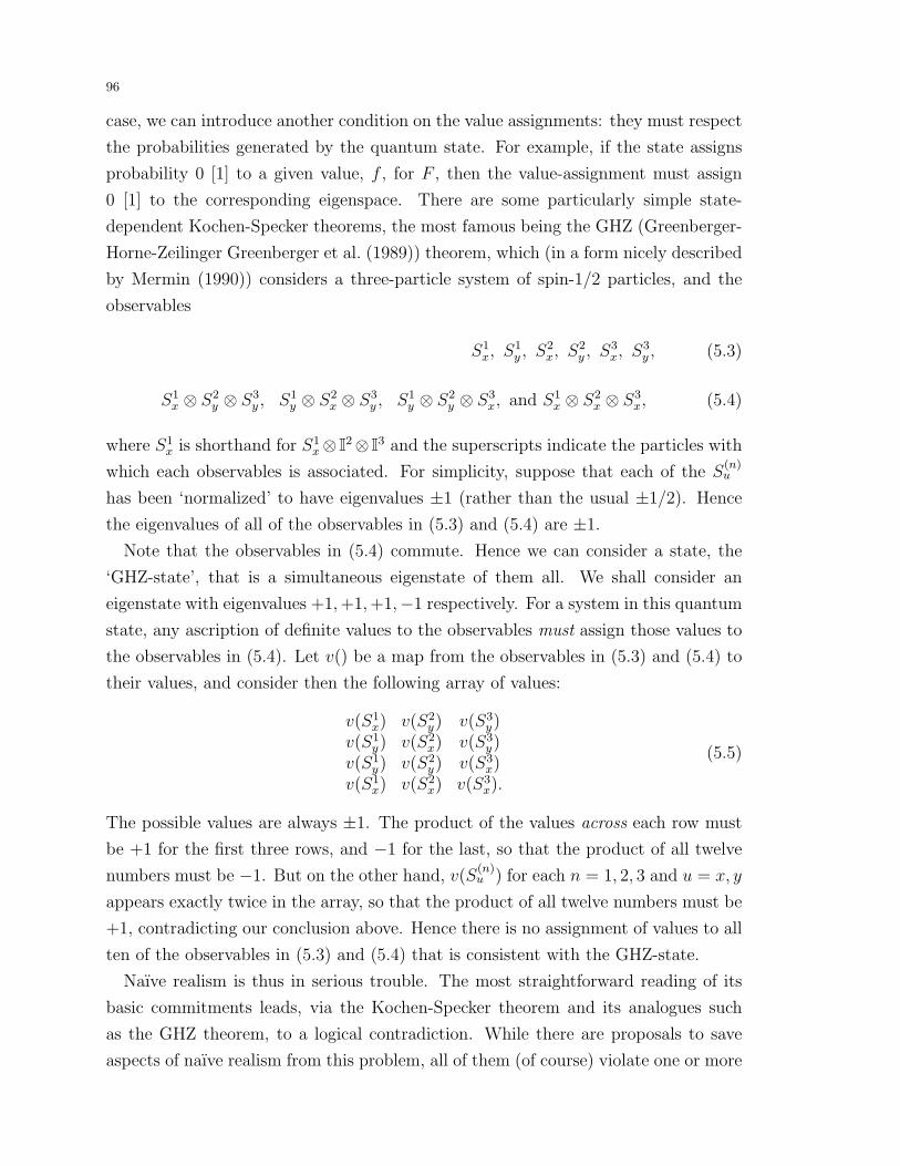
96

case, we can introduce another condition on the value assignments: they must respect

the probabilities generated by the quantum state. For example, if the state assigns

probability 0 [1] to a given value, f , for F , then the value-assignment must assign

0 [1] to the corresponding eigenspace. There are some particularly simple state-

dependent Kochen-Specker theorems, the most famous being the GHZ (Greenberger-

Horne-Zeilinger Greenberger et al. (1989)) theorem, which (in a form nicely described

by Mermin (1990)) considers a three-particle system of spin-1/2 particles, and the

observables

S1x, S

1y , S

2x, S

2y , S

3x, S

3y , (5.3)

S1x ⊗ S2

y ⊗ S3y , S1

y ⊗ S2x ⊗ S3

y , S1y ⊗ S2

y ⊗ S3x, and S1

x ⊗ S2x ⊗ S3

x, (5.4)

where S1x is shorthand for S1

x⊗ I2⊗ I3 and the superscripts indicate the particles with

which each observables is associated. For simplicity, suppose that each of the S(n)u

has been ‘normalized’ to have eigenvalues ±1 (rather than the usual ±1/2). Hence

the eigenvalues of all of the observables in (5.3) and (5.4) are ±1.

Note that the observables in (5.4) commute. Hence we can consider a state, the

‘GHZ-state’, that is a simultaneous eigenstate of them all. We shall consider an

eigenstate with eigenvalues +1,+1,+1,−1 respectively. For a system in this quantum

state, any ascription of definite values to the observables must assign those values to

the observables in (5.4). Let v() be a map from the observables in (5.3) and (5.4) to

their values, and consider then the following array of values:

v(S1x) v(S2

y) v(S3y)

v(S1y) v(S2

x) v(S3y)

v(S1y) v(S2

y) v(S3x)

v(S1x) v(S2

x) v(S3x).

(5.5)

The possible values are always ±1. The product of the values across each row must

be +1 for the first three rows, and −1 for the last, so that the product of all twelve

numbers must be −1. But on the other hand, v(S(n)u ) for each n = 1, 2, 3 and u = x, y

appears exactly twice in the array, so that the product of all twelve numbers must be

+1, contradicting our conclusion above. Hence there is no assignment of values to all

ten of the observables in (5.3) and (5.4) that is consistent with the GHZ-state.

Naıve realism is thus in serious trouble. The most straightforward reading of its

basic commitments leads, via the Kochen-Specker theorem and its analogues such

as the GHZ theorem, to a logical contradiction. While there are proposals to save

aspects of naıve realism from this problem, all of them (of course) violate one or more

97

of the conditions of the Kochen-Specker theorem, and, arguably, are no longer ‘naıve’

realism.

5.4.2. Ensemble Interpretations. Ensemble interpretations (e.g., Ballentine 1970) at-

tempt to avoid the measurement problem altogether by stipulating that quantum

states are not about individual quantum systems. They are essentially statistical, and

thus can be used to describe only ensembles of systems. Hence the state at the end

of a measurement ought not be thought of as describing a particular apparatus (and

measured system) at the end of a particular measurement, but all such apparatuses

(and measured systems) and the end of all such measurements.

There are two strains of this sort of interpretation in the literature, not always

distinguished. The first we might call ‘minimalist’: it is the deflationary view that

one can make sense of the quantum state (for example, at the end of a measurement)

only as the description of an ensemble of similarly prepared systems.

The second strain of the ensemble interpretation makes a stronger claim, namely,

something to the following effect: nothing more than the deflationary account of the

quantum state is needed; i.e., there is no scientific demand for a theory that describes

individual systems. On this view, such a demand is an artifact of a deterministic

world view, and the usual ’mysteries’ of quantum theory simply disappear once one

learns to live with statistical theories. However, most researchers in the philosophy

and foundations of quantum theory appear to be unconvinced.

Moreover, even the minimalist claim faces a problem, and the problem also shows

why the stronger claims are, at the least, in need of further development. The Kochen-

Specker theorem already shows that the probabilities generated by quantum states

cannot be understood straightforwardly as classical probabilities. Thus the ensemble

interpretations appear to be pushed towards other views, such as the quantum logic

view, which will be considered later.

5.4.3. Collapse Postulate. The ‘standard’ solution to the problem of measurement is

the so-called ‘collapse postulate’ (also called the ‘projection postulate’) of quantum

theory, already mentioned in §3.1.2, first discussed in detail by von Neumann (1932,

p. 351 and pp. 417-418 of the English translation). The postulate can be found

stated in numerous ways, such as:

Collapse Postulate: Upon measurement of the observable F on a system in

the state W , the result of the measurement will be an eigenvalue correspond-

ing to some eigenspace, P of F , and the state of the system will then be

PWP/Tr[PWP ].

98

If the state can be written as a vector, |ψ〉, then the ‘collapse’ amounts to projecting

this vector onto ranP , i.e., onto P |ψ〉, and renormalizing the result.

There are many reasons to be unhappy with the collapse postulate, but it is worth

saying, at the start, that most of the time, for most of the predictions that one wants

to make from quantum theory, the postulate works very well.

One often-cited problem with the collapse postulate is that it amounts to discontin-

uous (and irreversible) evolution of a system. The resulting picture of the evolution

of quantum systems is thus odd indeed: continuous, deterministic, reversible, unitary

evolution (through Hilbert space) according to the Schrodinger equation (or some

other quantum equation of motion), punctuated by discontinuous, irreversible, prob-

abilistic, instantaneous, changes of the state.

At the very least, one would like some story about why these punctuations occur.

Clearly, in the statement of the postulate, they are connected with measurement.

But what is physically special about measurement? Alas, no compelling answer is

forthcoming. Indeed, the most obvious problem with the collapse postulate is that it

relies on an unanalyzed notion of ‘measurement’. Most of the time, reasonable people

can agree about when a measurement has occurred, but that fact is entirely unhelpful.

For most researchers in the foundations and philosophy of quantum theory seem to

agree that if quantum theory is supposed to be a fundamental theory, then it should

tell us when a measurement occurs (or more generally, what a measurement is), not

vice versa. The world should not rely on us to ‘tell it’ when to collapse a state.

5.4.4. Macro-Micro Distinction. One answer to the question ‘what is a measurement’

is suggested by our discussion of Schrodinger’s cat (§5.1.1), and is sometimes put for-

ward as a response to the measurement problem. The suggestion is that a measure-

ment occurs when the state of a microscopic system is ‘magnified’ in such a way that

it becomes correlated with the state of some macroscopic system. There is no deny-

ing that paradigmatic measurements do have this feature. Alas, this characterization

relies on another ill-defined notion, namely, the difference between the microscopic

and the macroscopic.

The distinction is also sometimes made between the ‘easily reversible’ and the

‘esssentially irreversible’. Because microscopic systems have few degrees of freedom,

their behavior is often easy to reverse, while the behavior of macroscopic systems,

with vastly many degrees of freedom, is very difficult if not practically impossible to

reverse.

In either case—whether the point is made in terms of size or reversibility—the

idea is supposed to be that at an appropriately large (or irreversible) scale, physical

99

systems behave classically. Indeed, one sometimes hears ‘the Copenhagen’71 interpre-

tation of quantum theory, and especially Bohr’s version of it, characterized in this

way: one must presume that measuring apparatuses are classical objects, and this

presumption provides the grounds for determining when a collapse (measurement)

occurs.

However, while again providing an often useful practical characterization of mea-

surement and ‘the classical’, these distinctions are, in most researchers’ view, not well

enough defined to sit at the foundations of a supposedly fundamental theory.

5.4.5. Decoherence. A related idea, but recently more well developed, is that sufficient

interaction with ‘the environment’ serves, in essence, to ‘collapse’ (‘decohere’) the

state of a system. Here we need to be very careful, because there is a well-studied

phenomenon, called ‘decoherence’, that involves the interaction of a system with its

environment. There is no disputing the physical importance of this phenomenon.

On the other hand, many have invoked this phenomenon as providing some sort of

solution to the measurement problem. This claim requires careful scrutiny.

5.4.5.1. The Phenomenon of Decoherence.

5.4.5.1.a. Qualitative Description. It is remarkably difficult to isolate a physical sys-

tem from the rest of the world (its ‘environment’). Particles from almost every corner

of the particle zoo are hurling around, and a great many of them can penetrate even

very strong barriers (such as lead walls). Even for very small systems (such as a

particle of dust), it is well-nigh impossible to prevent significant interaction with the

environment.

Physicists have developed both simple and very sophisticated models of this inter-

action, ranging from assuming that the system interacts with an otherwise unspecified

thermal bath to carefully modeling the rate, nature, and strength of interactions that

a given system is likely to experience in a given type of environment. With these

models, one can estimate (and in very rare, usually highly idealized, cases, explicitly

determine) the effect of these interactions on the state of the system.

Notice that these interactions will entangle the system with the environment. We

are therefore no longer talking, in the first place, about ‘the’ state of the system,

but about the state of the composite ‘system-plus-environment’. Of course, typically

we will have little or no access to the relevant environmental degrees of freedom.

71This ‘interpretation’—unlikely, however, to have ever been a single unified view—is so-calledbecause it is typically associated with Niels Bohr and his associates, who worked in Copenhagen.See Cushing (1994, chs. 6,7), Beller (1999), and references therein, as well as Landsman, Ch. 4, §1,this volume.

100

(Imagine, for example, that a photon bounces off a dust particle, then gets trapped

in the atmosphere, or worse, heads out to space. In the former case, recovering the

photon will be practically impossible, and in the latter case, it could be literally

impossible.) Although these degrees of freedom in a sense ‘encode’ certain informa-

tion about the system (such as its location, because typically the interactions are

position-dependent), that information is almost always practically, and occasionally

in principle, lost to us.

Hence, although the system will become entangled with the environment, we typi-

cally have access only to its reduced state, not to the state of the total composite. We

obtain this reduced state by tracing out the degrees of freedom of the environment.

In many models of the interaction, the result is a reduced state for the system that

is approximately diagonal in position; that is, its (mixed) state looks like the state of

a system that is well-localized in space (in the sense that each component (spectral

projection) of the mixture is well-localized in space). Decoherence may, in this sense,

be thought of as ‘localizing’ the system (but see section 5.4.5.2.a, where we will worry

explicitly about the fact that this mixture is improper).

This localization ultimately derives from the fact that in these models, the interac-

tion between the system and the environment is position-dependent. (The environ-

ment interacts with the particle only in the vicinity of the particle.) More generally,

if the interaction Hamiltonian that describes the exchanges of energy between the

system and its environment commutes with some system observable, Q ⊗ I, then

the reduced state of the system becomes approximately diagonal in the basis picked

out by the eigenvectors (or eigenspaces) of Q. The environment is said to ‘suppress’

the off-diagonal, ‘interference’ terms. Moreover, because the interaction Hamiltonian

commutes with Q, a system that is already in an eigenstate of Q will tend to remain so

(assuming, as is often physically reasonable, that the interaction Hamiltonian swamps

the effects of the free Hamiltonian for the system).

5.4.5.1.b. Example. A classic and much-studied example of decoherence (e.g., Joos

and Zeh 1985), involves a dust particle in the atmosphere. Here is a simplified sum-

mary of their argument.

Let |ψ〉 represent the initial state of the dust particle. Let the states |ψq〉 be a basis

of well-localized states for the particle (each centered at a position labeled q). Let

|E0〉 be the initial state of the environment, and consider the interaction between the

particle and a single air molecule in the environment for a particle that is in one of the

states |ψq〉: as a result of this single interaction, we will assume that the particle-plus-

environment evolves into the state |ψq〉 ⊗ |Eq〉. (Here we assume, in particular, that

101

the dust particle is much heavier than the air molecule, so that the interaction leaves

the state of the dust molecule essentially unchanged). Joos and Zeh show, roughly,

that if |ψ〉 (represented as a wavefunction) is initially in a Gaussian (not necessarily

well-localized) state, written in the |ψq〉-basis as |ψ〉 =∑

q cq|ψq〉, then the matrix

representation of the reduced density operator for the particle in the |ψq〉-basis (recall

§1.2.3.4), after one such interaction, will be:

Wqq′ = cqc∗q〈Eq|Eq′〉, (5.6)

where |〈Eq|Eq′〉| ≈ 0 whenever the distance between q and q′ is much larger than

the wavelength of the dust particle.72 In other words, the off-diagonal (q 6= q′) terms

in Wqq′ get reduced by a factor of 〈Eq|Eq′〉. The intuition here is that because the

states |Eq〉 and |Eq′〉 correspond to environments where the air molecule has scattered

from the dust particle in two different locations (represented by q and q′), if those

locations are very different, then the corresponding states of the environment will be

‘very different’ (i.e., nearly orthogonal). (Of course, if q = q′ then this inner product

is 1.)

Joos and Zeh then show, for a wide range of different models of the environment,

that after many such interactions, the off-diagonal terms in the reduced density matrix

decay exponentially, at a rate that depends on q − q′ (and is zero when q = q′). The

rate is very fast: according to Joos (1986), the reduced density operator for a dust

particle with radius 10−5cm in even a high quality vaccuum will be extremely close

to diagonal in position73 in about one microsecond. One says that the state of the

object system (the dust particle) has ‘decohered’ as a result of its interaction with

the environment.

5.4.5.2. Decoherence and the Measurement Problem.

5.4.5.2.a. Decoherence Does not Solve the Problem. Decoherence appears to ‘localize’

systems that interact with their environment, so that perhaps we will not, after all,

ever need to worry about encountering cats that are ‘smeared’ between two macro-

scopically distinct states (recall §5.1.1). Alas, there is a problem with this conclusion,

stemming from the fact that the reduced state of the system is an improper mixture

(recall §1.2.6.3.b). Let us investigate this point further.

On the one hand, we must acknowledge that it would be practically impossible

to perform an experiment to determine that the reduced state of a system that has

72Here we are relying on de Broglie’s relation between momentum and wavelength—recall note58 of §4.2.1.

73In this case, ‘extremely close to diagonal in position’ means that the reduced density operatorcan be written as a sum of states that represent the dust particle localized to within about 10−13cm.

102

decohered is not a proper mixture. To see why, consider the very simple case of two

perfectly correlated particles (analogous to the object system and its environment,

which, as a result of their interaction, have become correlated), as in (4.10). The

reduced state for α is Wα =∑

n(1/N)|an〉〈an| (analogous to the reduced state of the

object system, which, recall, is ‘nearly diagonal in position’). This state makes the

same predictions for every observable on α as the state in (4.10) does. In order to

distinguish between proper and improper Wα, we would therefore need to measure

some observable on the compound system (α&β), and in particular we would need

to measure the correlations between α and β (for α & β is not in an entangled state–

and therefore α’s state is a proper mixture—if and only if there are no non-trivial

correlations between them). Now, in the case of (4.10), measuring these correlations

is relatively straightforward (assuming that we have many copies of the pair all in the

same state), because in fact they are perfectly correlated in many observables. But in

the case of interest here—an object system and its environment—things are decidedly

more difficult, because the correlations exist only between a very few particles of the

environment and the object system. As I noted above, it is in general practically

impossible to recover those particles from the environment, and even if we could, in

general not just any measurement on them will do the job. Indeed, if we do not have

many copies of the total system (and in general we will not!), then the measurement

in question becomes even more difficult, because we must measure an observable

(analogous to the projection onto the state in eq. 4.10) that is not even a product

(i.e., of the form F ⊗G).

On the other hand, the practical impossibility of performing such a measurement

on the environment does not by itself license the assumption that the mixed state

of the decohered system is (or may be treated as if it is) proper. The problem,

as ever, is the eigenstate-eigenvalue link. The true quantum-mechanical state of the

compound system is an entangled state, and in this state, according to the eigenstate-

eigenvalue link, the object system does not have a definite location (in general).

The assumption that the state of the system ‘might as well’ be a proper mixture

is in fact inconsistent with this claim. In other words, while the two states are

observationally very hard to distinguish, they are (given the eigenstate-eigenvalue

link) interpretationally inconsistent.

Of course, one could give up on the eigenstate-eigenvalue link, and many inter-

pretations do. We will discuss some of them shortly. The point here is that, with

the eigenstate-eigenvalue link in place, decoherence does not solve the measurement

problem.

103

5.4.5.2.b. Decoherence Does Help with the Problem. Decoherence does, however, help

with the most general form of the problem of measurement. Recall (§5.3.2) that the

measurement problem is not confined to interactions that would typically be regarded

as measurments. Many interactions between quantum and macroscopic systems will

put the macroscopic system in a state that, given the eigenstate-eigenvalue link, will

be contrary to what most presume to be the deliverances of everyday experience. In

other words, in its most general form, the ‘measurement’ problem is just the problem

that quantum theory apparently fails to assign definite values to observables that

appear, on the basis of everyday observation, to have definite values. In the special

case of a typical measurement, we are perhaps already halfway to a solution, for in

this case, the apparatus is at least already in a mixture, albeit improper, of ‘desired’

states.

But what about the more general sorts of interactions, mentioned above, that are

not explicitly measurements but still generate ‘bad’ states for macroscopic objects?

Decoherence promises to secure the following: for ‘relatively large’ systems (for ex-

ample, at least as big as a dust particle), interaction with the environment will entail

that the state of the system will become a mixture, albeit improper, of ‘desired’ states

(or something that is very close to such a mixture—so close that one might be willing

to overlook the difference). Even so, however, this strategy has merely reduced the

general problem to a problem that continues to elude a satisfactory solution, although

it does give one further justification for focusing the discussion specifically on mea-

surements (because decoherence apparently reduces the general situation to one that

is at least formally similar to measurement-situations).

5.5. Interpretations.

5.5.1. Ways of Pursuing the Project. I have covered a number of philosophical and

foundational issues arising from quantum theory, and an ‘interpretation’ of the theory

should address all of them in some way or other—from providing an account of the

empirical content of the theory, to providing an understanding of incompatibility

(and thereby the ‘uncertainty relations’), to providing some understanding of the

apparent failure of locality in the theory (§6). Nonetheless, most interpretations

are aimed primarily at solving the measurement problem. As we saw above, that

problem can be characterized (among other ways) as a conflict between (i) a common

understanding of the physical properties of familiar physical objects, including the

sorts of inferences about them that are valid, and (ii) a minimal account of when

observables are empirically well-defined, taken in the context of (iii) quantum theory.

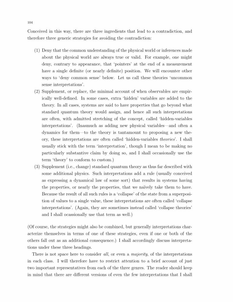
104

Conceived in this way, there are three ingredients that lead to a contradiction, and

therefore three generic strategies for avoiding the contradiction:

(1) Deny that the common understanding of the physical world or inferences made

about the physical world are always true or valid. For example, one might

deny, contrary to appearance, that ‘pointers’ at the end of a measurement

have a single definite (or nearly definite) position. We will encounter other

ways to ‘deny common sense’ below. Let us call these theories ‘uncommon

sense interpretations’.

(2) Supplement, or replace, the minimal account of when observables are empir-

ically well-defined. In some cases, extra ‘hidden’ variables are added to the

theory. In all cases, systems are said to have properties that go beyond what

standard quantum theory would assign, and hence all such interpretations

are often, with admitted stretching of the concept, called ‘hidden-variables

interpretations’. (Inasmuch as adding new physical variables—and often a

dynamics for them—to the theory is tantamount to proposing a new the-

ory, these interpretations are often called ‘hidden-variables theories’. I shall

usually stick with the term ‘interpretation’, though I mean to be making no

particularly substantive claim by doing so, and I shall occasionally use the

term ‘theory’ to conform to custom.)

(3) Supplement (i.e., change) standard quantum theory as thus far described with

some additional physics. Such interpretations add a rule (usually conceived

as expressing a dynamical law of some sort) that results in systems having

the properties, or nearly the properties, that we naıvely take them to have.

Because the result of all such rules is a ‘collapse’ of the state from a superposi-

tion of values to a single value, these interpretations are often called ‘collapse

interpretations’. (Again, they are sometimes instead called ‘collapse theories’

and I shall ocassionally use that term as well.)

(Of course, the strategies might also be combined, but generally interpretations char-

acterize themselves in terms of one of these strategies, even if one or both of the

others fall out as an additional consequence.) I shall accordingly discuss interpreta-

tions under these three headings.

There is not space here to consider all, or even a majority, of the interpretations

in each class. I will therefore have to restrict attention to a brief account of just

two important representatives from each of the three genres. The reader should keep

in mind that there are different versions of even the few interpretations that I shall

105

discuss here. In most cases, I have chosen to describe a version that strikes me as the

least problematic, but this claim is, in most cases, controversial.

My treatment of these interpretations will, necessarily, be brief. I will give a few

more references than normal, to get the interested reader started on the literature.

5.5.2. ‘Uncommon Sense’ Interpretations.

5.5.2.1. Quantum Logic Interpretations. I have already noticed (§2.1.1) that the lat-

tice of subspaces of a Hilbert space, i.e., the lattice of ‘propositions’ about a physical

system, can, prima facie, be interpreted logically. Quantum logic interpretations take

this idea seriously, and understand quantum theory to necessitate a revolutionary

change from classical to quantum logic.74

One way to characterize the difference between classical and quantum logic is in

terms of the failure of distributivity (§7.4.3)—the classical and quantum lattices of

propositions are otherwise structurally (logically) the same. The basic idea of the

quantum logic interpretation, then, is that in particular the classical law of distribu-

tivity is invalid. This invalidity is supposed to allow one to make the sorts of assertion

tha, for example, the naıve realist (§5.4.1) had hoped all along to be able to make.

For example, let F and G be two incompatible maximal observables sharing no eigen-

vectors. Denote their eigenspaces by {Fn} and {Gm}. As propositions (elements of

the lattice of subspaces of the Hilbert space, interpreted logically), they assert that a

system has the corresponding eigenvalue as a value for the observable. Then:(∨n

Fn

)∧

(∨m

Gn

)= I ∧ I = I (5.7)

where I is the logically true proposition. If we read the first half of this conjunction

as asserting that the observable F has some value (understanding the existential

quantifier in terms of disjunction, as one often does), and similarly for the second

hand of the conjunction, then (5.7) asserts that F has a value and G has a value.

Indeed, this assertion is logically true. (Note that if we could apply distributivity to

(5.7), then we could quickly turn it into a logical contradiction, because for any n

and m, Fn ∧Gm = 0, the logically false proposition.)

74 Birkhoff and von Neumann (1936) were among the earliest advocates of something like aquantum logic interpretation. Subsequent work in this area is founded on theirs. Some of theadvocates of a quantum logic interpretation have been: Finklestein (1962; 1969), Putnam (1969),Friedman and Putnam (1978), and Bub (1974). See also the collection of papers (Hooker 1975,1979).Some well-known critiques have been made by Dummett (1976) and Gibbons (1987). Many ofthe standard objections are addressed in Dickson (2001), and occasionally also in the work of theadvocates listed above.

106

Moreover, the corresponding claim is true for a similar conjunction (∧) of such dis-

junctions for any number of observables. Hence (understanding the universal quan-

tifier in terms of conjunction) the quantum logic interpretation claims to recover the

idea that all observables (for a given system) always have a value (for that system).

If so, then the measurement problem is no longer a problem. Of course, this approach

also raises some questions. In addition to doubts about whether logic is revisable at

all, some have argued that the quantum logic interpretation simply moves the mystery

from one place (quantum theory) to another (logic). In any case, it is clear that the

quantum logic interpretation needs to make some argument about why classical logic

does in fact work within certain domains. (Decoherence could be helpful, here.) It

also needs to say something about the success of classical reasoning in mathematics.

Both of these projects amount to open questions in the quantum-logic interpretation

(Dickson 2001).

5.5.2.2. Many-Somethings Interpretations. Our second example of ‘uncommon-sense’

interpretations is the ‘many-somethings’ interpretations. These interpretations gen-

erally go under the heading ‘many-worlds’ interpretations, but the notion of a ‘world’

that is at work here (quite problematic in its own right) is sufficiently far from the

usual understanding of that term that a less committal word seems appropriate.75

In any case, whereas quantum-logic interpretations deny (or at best re-interpret)

the logical validity of apparently valid inferences about the properties of physical

objects, many-somethings interpretations deny (or at best re-interpret) the truth of

apparently true claims about the properties of physical objects.

Consider again the right-hand side of (5.2). The problem that this state raised

earlier was that, on the standard interpretation (adopting the eigenstate-eigenvalue

link), a (compound) system in this state has no particular value for the observable

F ⊗Q (where Q is the pointer-observable). The many-somethings interpretations go

to the opposite extreme, and claim that every term on the right-hand side is ‘real’,

corresponds to some reality. The apparatus has neither zero, nor one, of the values

for the pointer-observable, but all of them.

Immediately, these interpretations face some questions. There is, of course, the

obvious question of how systems can manage to ‘have’ multiple states—it appears

75Indeed, we are talking, here, about a rather wide class of interpretations. It is far from clearthat the intention of the originator of this class of views, Everett (1957), was to invoke the ideaof many worlds, which appears to have been introduced by DeWitt (see his, and Everett’s, articlein DeWitt and Graham, 1973). A ‘many-minds’ variant has been proposed by Albert and Loewer(1988) and Donald (1990), among others. See the review by Butterfield (1995) and the book byBarrett (1999) for finer-grained classifications and many references.

107

to involve a straightforward contradiction. Generically, the reply is to introduce an

indexical property that resolves the contradiction—the different values of the pointer-

observable, for example, are realized relative to different values of the indexical prop-

erty, which correspond to different somethings (‘worlds’, or in some versions, ‘minds’).

Everett’s original idea, however, seems rather to have been fundamentally rela-

tional in character. Indeed, consider a generic two-system state, as in (1.26). If

the first system might be said, in some sense, to ‘really have’ the state |xj〉, then

relative to |xj〉, the second system might be said to be in the state |ψrelative to xj〉 =

Kj

∑m cjm|ym〉, where Kj is some constant of normalization. The probabilities gener-

ated by |ψrelative to xj〉 for the results of measurements on the second system are exactly

those generated by the original compound state (for measurements that are restricted

to the second system). Everett’s original idea seems to have been that systems posses

states only ‘relative’ to the states of other systems. Others seem to adopt something

like the view that the first system has various of the |xj〉 in different ‘worlds’, and in

those worlds, the second system has the corresponding relative state.

Each of these views raises difficult questions. In the case of Everett’s relational view,

more needs doing. Consider the analogous case in space-time theories, where (prior

to the 20th century), relationalists asserted that the only (spatio-temporal) reality

is relational, but the only theory that was available (Newtonian classical mechanics)

was not explicitly relational.76 Everett’s relational view seems to be in somewhat of a

similar situation. (For example, how and from what ‘point of view’ does the quantum

state for the compound system itself get assigned? And how can it be understood

relationally?) The many-somethings views face the obvious metaphysical hurdle of

making some sense of the plurality of ‘somethings’ (worlds, minds, whatever).

Here, I will raise just one additional question, commonly raised. The general pre-

scription of these interpretations is to allow that every term in a superposition cor-

responds to a ‘reality’, in the sense just described. But recall that a given state can

be decomposed in many ways, and that in general the terms in the superposition are

different, depending on the decomposition. Which decomposition is ‘correct’?

One sort of answer to this question will postulate, or argue for, a preferred basis,

in terms of which the decomposition is to be made. (The argument for a preferred

basis is most often made on the grounds that decoherence (§5.4.5) picks it out, but

there is a serious question whether the near-diagonality in position that decoherence

76See, for example, Brown and Pooley (2002) for details of the history, and see Butterfield, Ch.1, §2.3, this volume, for further discussion of relationalism.

108

typically effects is sufficient.77) This answer is, in any case, highly problematic. For

suppose that we had some good reason to believe that there is a preferred basis whose

elements represented the true physical properties of all objects. In that case, we would

hardly need the extravagance of the many-somethings interpretations to resolve the

measurement problem. Relying on the preferred basis, we would simply assert that

systems are always to be described in terms of this basis. There would then be no

obstacle (for example, no Kochen-Specker contradiction) to defining probabilities over

the properties picked out by this basis. (Indeed, below (§5.5.3.1) we will consider an

interpretation—the de Broglie-Bohm theory—that can be characterized in precisely

these terms.)

Another answer allows all decompositions to correspond to realities. Here, deco-

herence can be helpful, because it suggests that creatures like us, that is, creatures

who interact with their environment in the particular way that we in fact do, will in

fact be subject to decoherence, so that our perceptions will be correlated to the ‘right’

states of the objects of our perception, and we, as perceivers, will, as far as we can

tell (with very high probability) be in worlds where the properties are the ones we

typically believe objects to have. Of course, there remains to explain the point that

in fact there are many ‘copies’ of each one of us (one for each value of the indexical),

but we leave that issue to the advocates of these interpretations, who have their own

ways of making sense of this type of plurality.

5.5.3. ‘Hidden-variables’ Interpretations. Ths basic idea behind any hidden-variables

interpretation is that quantum theory (as EPR argued!—§4.4) is incomplete. These

interpretations propose to supplement the state assigned to a system by quantum

theory with an additional, ‘hidden’, state. (The variables need not in any sense be

unavailable to observation; they are ‘hidden’ only from the eyes of quantum theory.)

Of course, not just any proposal will do. In particular, such theories must somehow

recover the empirical success of quantum theory. Doing so amounts to recovering the

quantum probabilities as an average over the hidden states, in much the same way that

one hopes to recover classical thermodynamics from classical statistical mechanics by

averaging over the micro-states of the system. (See Uffink, Ch. 9, this volume.)

Hence, for example, label the hidden states by λ (where for simplicity we will assume

that λ ∈ R). Let ρW () be the distribution of the hidden states in the (quantum) state

W . Finally, let Prλ,W (F = fk) be the probability assigned by the hidden state λ to

77It is worth noticing as well that a state’s being nearly diagonal in position does not entail thatthe basis in which is is diagonal is anything close to position. See Bacciagaluppi (2000). In thesecases, which basis are we to say is ‘picked out’ by decoherence?

109

the result (eigenvalue) fk of a measurement of F on a system in the state W . (In the

deterministic case, all such probabilities are of course 0 or 1.) Empirical adequacy

then requires that ∫RρW (λ)Prλ,W (F = fk)dλ = Tr[WPfk

], (5.8)

where Pfkis the eigenspace of F corresponding to the eigenvalue fk.

In this section, I will consider the de Broglie-Bohm theory (§5.5.3.1), a deterministic

hidden-variables theory, and modal interpretations (§5.5.3.2), which are in general

indeterministic.

5.5.3.1. The Theory of de Broglie and Bohm. The de Broglie-Bohm theory is a deter-

ministic theory of the trajectories of particles, somewhat in the mold of classical New-

tonian (better, Hamiltonian) dynamics.78 In its original form, the hidden-variables

theory was formulated explicitly by dividing the Schrodinger equation (including a

potential, V , in the Hamiltonian) into a real and complex part, so that the solu-

tion, ψ(x, t), is written as ψ(x, t) = R(x, t)eiS(x,t). The complex part has the form of

Hamilton’s equations of motion, with an extra term in the expression for the potential

energy, the ‘quantum potential’:

∂S

∂t+

(∇S)2

2m+ V − 1

2m

∇2R

R= 0 (5.9)

This equation has the form of Hamilton’s equation, with the potential given by V +

U where U is the ‘quantum’ potential − 12m

∇2RR

. The real part has the form of a

continuity equation, and implies the conservation of probability:

∂p

∂t+∇ · pq = 0, (5.10)

where p(x, t) = R2(x, t) = |ψ(x, t)|2 is understood (stipulated to be) the probability

of finding a particle at the point x (at time t) and

q(x, t) = ∇S(x, t)/m (5.11)

is interpreted as the velocity of the particle (when it is at the point x and time t).

Hence, one can understand the one-particle Schrodinger equation as describing

an ensemble of particles (each of whose ‘quantum state’ is the same), distributed

(in space) according to p(x, t). By (5.10), this distribution is conserved over time,

and thus may be understood properly as a probability distribution. The individual

78The basic idea was first suggested by de Broglie, most famously in his (1927). Later (after deBroglie had been convinced that the theory does not work) it was developed by Bohm (1952), andhas seen much further development in the past few decades. For a variety of approaches to andviewpoints on the theory, see Cushing, Fine, and Goldstein (1996).

110

particles move as if they were classical particles governed essentially by Newton’s laws

with the usual classical potential plus the additional ‘quantum potential’, U .

This theory is important for several reasons. Here I will mention three.

First, it shows that the eigenstate-eigenvalue link is far from a required principle

of interpretation. Indeed, the eigenstate-eigenvalue link is quite strongly denied in

this theory. The position observable does not even have eigenstates, and yet, on this

theory, every particle always has a definite position.

Second, it provides a clear counter-example to oft-cited lessons of quantum theory,

to the effect that quantum mechanics implies a lack of determinacy at the fundamen-

tal level, the impossibility of fundamental determinism, the impossibility of definite

trajectories for particles, the impossibility of picture quantum phenomena, and so on.

The theory clearly describes particles with definite trajectories, moving deterministi-

cally under the potential V + U .

Third, this theory is probably the best-developed interpretation, with applications.

There are compelling accounts of how particles behave during measurements of spin,

for example (Dewdney, Holland, and Kyprianidis, 1986). Moreover, the theory has

occasionally been used to make headway on applications and problems that seemed

much more difficult from the standard point of view. A nice example involves the

prediction of how long a particle that will tunnel through a potential barrier will spend

in the barrier. This quantity is conceptually tricky (at best) in standard quantum

theory, because the ‘particles’ have no definite trajectories, and there is no time

observable in quantum theory. But the problem is conceptually straightforward within

the de Broglie-Bohm theory (Leavens 1990), precisely because one can essentially

display the possible trajectories of a particle under the influence of the potential

barrier (and the quantum potential), and then simply take the average of the times

spent in the barrrier.

However, we should not ignore some difficult issues faced by the theory. Setting

aside (as outside the purview of this article) the (very significant) difficulty of extend-

ing the basic idea to relativistic quantum field theory, there are other questions that

it faces. Here I will mention one.

Initial appearances notwithstanding, the ontology of the theory can stretch the

imagination a bit. Indeed, one faces the following dilemma. One the one hand, if we

take the ‘guiding field’ (quantum potential) to be a real potential field of some sort, it

is highly non-local. (In the literature, this point is sometimes put in terms of the fact

that it ‘lives’ not in R3, but in the configuration space for the multi-particle system;

of course, for a one-particle system they are the same.) This point gets reflected in

111

the form of the ‘guidance condition’ (5.11) for many particles: qi(x1, x2, . . . xn, t) =

∇iS(x1, x2, . . . xn, t)/mi. That is, the velocity of particle i depends not only on its

location, but also on the location of the other particles. Finally, notice that the

particle does not respond to the intensity of the quantum potential in its region, but

to the form. That is, increasing the intensity of the quantum potential (multiplying

R in (5.9) by some constant > 1) does not change its effect on the particles at all.

All of these (and more) observations will, for some, add up to the conclusion that the

quantum potential is, at best, in need of some serious metaphysical clarification, and

at worst, too bizarre to countenance.

On the other hand, one might then deny its reality. A particle moving according

to the guidance condition, with V = 0 (zero ‘classical’ potential) will in general

still ‘deviate’ from the classically expected trajectory, but are we thereby required to

suppose that this ‘deviation’ is due to the presence of some additional, non-classical,

potential? Perhaps, instead, we can take the guidance condition as a fundamental

rewriting of Newton’s laws.79 In this case, we may avoid the oddness of the quantum

potential as a physical entity, but the theory becomes extremely reductionistic—the

only real property of particles is their spatio-temporal trajectory. Such a theory

is forced to eschew providing explanations (for phenomena such as bonding between

particles) that one might wish to have, and in general we do have in standard quantum

theory.80

5.5.3.2. ‘Modal’ Interpretations. Model interpretations81 are in many ways similar

to the de Broglie-Bohm theory: they also postulate hidden-variables (denying the

eigenstate-eigenvalue link) and they also (at least, they can formulate a dynamics

for these hidden-variables. There are two major differences: (1) in general model

interpretations will allow that the physical quantities that are ‘definite’ for a sys-

tem are state-dependent, and therefore they can change in time; (2) in general (and

typically as a consequence of the choice they make for which physical quantities are

definite) model interpretations are stochastic. Many such interpretations have been

79Indeed, the basic idea here is to reform the very notion of an ‘inertial’ trajectory. See Pitowsky(1991.

80See Bedard (1999 and Dickson (2000.81There are many variants on the general theme of modal interpretations. The term itself was

coined by van Fraasen (1972). A renaissance of sorts occurred in the 1980s, with, for example,key works by Kochen (1985), Dieks (1988), and Healey (1989), and a later related but somewhatdifferent view put forward by Bub (1997). A helpful monograph is Vermaas (2000), and a helpfulcollection is Dieks and Vermaas (1998).

112

proposed. Here we concentrate one class of such interpretations (‘spectral modal in-

terpretations’) that has seen much development, and briefly refer to some more recent

ideas.

Recall that every density operator can be uniquely decomposed as a weighted sum

of its spectral projections. The central claim of spectral modal interpretations is that

the set of observables with a definite value is the largest set that can consistently

be assigned values, with the restriction that the spectral projections of the density

operator must have values (0 or 1, in this case). In other words, treat the density

operator as an observable, and assign it a value; then assign values to as much else

as one can without running into a Kochen-Specker-type contribution. It turns out

that, under some reasonable assumptions, this idea leads, for any given state (density

operator), to a unique set of observables that will get assigned a definite value.82

Because the state (of course) changes in time—and keep in mind that we are talking

about the reduced density operator, so that it need not change unitarily—the definite-

valued observables generally change in time.

Many (though not all) modal theorists aim to define some sort of dynamics for the

definite properties of a system. The problem is complicated because there are two

sorts of dynamics occurring ‘together’: (deterministic) changes in the set of definite-

valued properties (observables) for a system, and (stochastic) transitions from one

definitely possessed property to another. It was shown by Bacciagaluppi and Dickson

(1999) that the problem has a solution, and they exhibit some examples. However,

just as in Bohm, there arises a serious difficulty about whether such a dynamics can

be made Lorentz-invariant. Straightforward generalizations from the non-relativistic

to the relativistic case are known to be unavailable, but it remains an open question

whether a ‘natively’ relativistic version of the approach can work. The resolution

of this issue is connected with the more general issue of whether, and if so how, the

basic idea of the modal interpretation (‘make as many observables definite as possible,

given certain constraints’) can be extended to quantum field theory. If it can, it seems

that the most likely venue will be that of algebraic quantnum field theory, for even

the non-relativistic quantum-mechanical versions of the modal interpretation lend

themselves nicely to an algebraic formulation.83

82As an example of this genre of theorem, see Clifton (1995). Bub and Clifton (1996) prove asimilar theorem, but geared towards Bub’s (1997) interpretation.

83For example, see Halvorson (1999). For an initial foray into modal interpretations of quantumfield theory, see Clifton (2000). For a discussion of this foray especially as it relates to the issue ofLorentz-invariance, see Earman and Ruetsche (2006), which also includes references to the earlierwork on Lorentz-invariance in modal interpretations.

113

Do modal theories solve the measurement problem? If so, they do because their

prescription for choosing the definite-valued observables manages to pick out the

observables—such as pointer observables—whose definiteness is threatened by the

measurement problem. The de Broglie-Bohm theory (as well as the modal interpreta-

tion of Bub 1997) accomplishes this feat more or less by fiat. So long as the properties

we believe pointers (and cats, and so on) to have can ultimately be understood to

supervene on the trajectories of the constituent particles, the de Broglie-Bohm theory

has a convincing solution to the measurement problem. Modal interpretations must

in general argue their way to this point. For example, is definiteness of the spec-

tral projections of the reduced density operator enough to secure definiteness of the

properties that we believe macroscopic objects have? This question, as it turns out,

is quite difficult to answer. In the case of an idealized impulsive measurement, the

reduced density operator for the apparatus does have the definite pointer-states as

its spectral projections. But in realistic (non-ideal) measurements, there is potential

trouble. At one time, it was thought that decoherence saves the day, but it is no

longer clear whether decoherence does the work needed here.84

5.5.4. Collapse Interpretations.

5.5.4.1. Non-Dynamical Collapse Theories. The idea that the quantum state must,

in some sense or other, ‘collapse’, is quite natural as soon as one interprets it in terms

of probability. And various suggestions have been made, from time to time, about

when this collapse occurs. See, for example, Dirac (1930)

Consider an observation, consisting of the measurement of an observ-

able α, to be made on a system in the state ψ. The state of the system

after the observation must be an eigenstate of α, since the result of a

measurement of α for this state must be a certainty.

That is, collapse occurs upon observation (i.e., measurement). The argument that

Dirac is making here is the following. If we repeat the measurement of α on the

system, we will get the same result that we got the first time (regardless of ψ, and

assuming, of course, that the measurement was of the first kind—§) with probability

1. Suppose that result was a. There is only one state that assigns probability 1 to a,

namely, the eigenstate corresponding to a.

84See Bacciagaluppi and Hemmo (1996) for the former attitude, and Bacciagaluppi (2000) for thelatter.

114

I have already suggested (§5.4.3) that an account along these lines is, at best, in

need of help.85 Otherwise, it is little more than a statement of the collapse postulate,

with no clear account of what makes the difference between ‘measurements’ and other

interactions.

One obstacle to drawing this distinction in a principled way is that if too few

interactions count as measurements, then we might, after all, still be stuch with the

measurement problem (because collapse might not occur in situations where we need

it to get the definiteness of properties that we experience as definite). However, if

too many interactions count as measurements, we might end up with a theory that is

empirically false. (For example, if the state of a photon passing through the double-

slit apparatus (figure 3) always collapses after it passes through the barrier, then we

will never see an interference pattern, contrary to experimental results.)

One approach to drawing the distinction (between cases where collapse occurs

and cases where no collapse occurs) that arguably avoids both of these pitfalls, and

arguably does begin to smell like interpretation of the theory, is due to Wigner

(1961). Wigner is motivated by the following argument, often referred to by the

name ‘Wigner’s friend’.

Wigner asks us to imagine the following scenario. A measuring apparatus, µ,

measures some observable, F (by means of a pointer-observable, M), on an object-

system, σ. Meanwhile, both Wigner (α) and his friend (β) are in a position to observe

µ (by means of ‘observation-observables’ A and B). Let us use |mn〉 to refer to the

eigenstates of M , and similarly for the rest.86 Now, suppose that the measurement

of σ by µ has occurred, while neither α nor β has observed µ. If σ was originally in

the state∑

n cn|fn〉 then we may write the state of the total system as∑n

cn|fn〉|mn〉|a0〉|b0〉 (5.12)

According to the eigenstate-eigenvalue link, in this state, µ and σ are not in a definite

states of M ⊗ F . At this stage, standard quantum theory will say to invoke the

collapse postulate, so that the state becomes |fk〉|mk〉|a0〉|b0〉 for some k. In other

words, in absence of specific knowledge about the outcome, the state becomes the

(ignorance-interpretable) mixture∑n

|cn|2Pfn ⊗ Pmn ⊗ Pa0 ⊗ Pb0 . (5.13)

85And, alas, such help has only rarely been forthcoming. Hence I have no list of references tooffer the reader, here. Perhaps the most famous attempt to make sense of non-dynamical collapseis precisely the one discussed here, due to Wigner.

86There is a serious question whether a physical state such as ‘observes the pointer to be in thestate |Mn〉 is pure, and therefore whether there are observables such as A and B. See §1.4.3.

115

However, as noticed above (§5.4.5.2.a), there is a real empirical difference between

(5.12) and (5.13), even if in general it is practically impossible to detect. Wigner

finds nothing in the nature of σ, µ, or the interaction between them, to warrant the

assumption that this physical change of state occurs.

Notice, moreover, that the observers α and β have not yet entered the picture in

a substantial way. But it is their definite experiences that we are (in this argument)

obligated to secure. Wigner considers himself (α), and notices that at this stage of the

process (i.e., once the state is given by eq. 5.12), nothing threatens the definiteness

of his experiences—in fact, he remains in the ‘has not yet observed’ state (|a0〉) with

probability 1. So consider the state after α observes the apparatus:

∑n

cn|fn〉|mn〉|an〉|b0〉. (5.14)

Now Wigner feels compelled to assent to collapse, because otherwise (by the eigenstate-

eigenvalue link) his own state would be indefinite.

But what about Wigner’s friend (β)? Suppose that β observes the apparatus before

α. Wigner argues that, given a principle of charity about β’s reports of prior mental

states, he is obligated to collapse the state upon observation by β, even if he (α) has

not yet observed µ. For suppose that α then (after β) observes µ, and then asks

β: After you observed µ, did you feel that you experienced a definite outcome? Did

you observe it to be in a definite state? Surely β will answer ‘yes’, and assuming (as

Wigner does—this assumption is the principle of charity) that we are to believe β’s

report, we must assume that the state collapse upon observation by β.

Hence any observer to whom the principle of charity applies will effect a collapse

of the state, upon observation. Wigner believe that the principle extends to anything

that is, or has, a ‘mind’ (a term that is largely uncircumscribed, here). Moreover,

given a fairly strong distinction between physical bodies and minds (i.e., given some

form of dualism), one can point to the distinctness of minds as somehow the reason

that observation by a mind collapses the state, while observation by a non-mind (e.g.,

a typical measuring apparatus) does not collapse the state.

Setting aside the question of the plausibility of the premises of Wigner’s argument,

notice that we have arrived at this conclusion through the backdoor. In other words,

Wigner does not give us an argument that proceed from the nature of minds, and

appeals to that nature to argue that observation by a mind will collapse the physical

state. Indeed, Wigner’s view faces the same difficulty that all dualisms face: what

is the connection between mind and matter? How does mind collapse the physical

116

state of a system? Various extraordinarily speculative ideas have been floated, none

particularly convincing. (See Atmanspacher 2004 for a review.)

5.5.4.2. Dynamical Reduction Theories. Another strategy for making collapse well-

defined is to describe it as a physical process. Of course, in one sense it already has

been characterized as a physical process, for it is a change in the physical state of a

system. Here, however, I mean something more, namely, formulating a single equation

of motion that somehow incorporates both the continuous ‘Schrodinger’ evolution and

collapse, in a unified way. There have been (and continue to be) many proposed

schemes along these lines.87 Here, again, I consider just one example.

5.5.4.2.a. Intuitive Account of Continuous Spontaneous Localization. The example

that I will consider is the continuous version of a theory originally proposed by Ghi-

rardi, Rimini, and Weber (1986). The continuous version, called ‘continuous sponta-

neous localization’ (CSL), is due to Pearle (1989). It is easiest to state in terms of

wavefunctions. The basic idea is that each physical system in the universe experiences,

simultaneously, two types of evolution: the ‘normal’, deterministic, ‘Schrodinger evo-

lution’, and a stochastic tendency towards localization. By the latter, we mean that

the system’s wavefunction (in configuration space) experiences random (but infinitesi-

mally small) fluctuations, the net result of which is, on average and with overwhelming

probability, to tend to make the wavefunction more localized—more of the probability

gets concentrated in some localized region.

The strength of this stochastic evolution, which determines how quickly the local-

ization occurs, is determined by the number of particles in the system.88 For systems

with microscopic numbers of particles, the stochastic part of the evolution is swamped

by the Schrodinger evolution, so that the evolution is, for such systems, nearly iden-

tical to that given by standard quantum theory. But for systems with macroscopic

(e.g., around 1023) numbers of particles, if the system is initially in a superposition of

two (or more) localized states whose centers of localization are far apart (> 10−5cm

or so), then the stochastic element of the evolution acts very quickly to suppress

(continuously) all but one of the terms in the superposition. The parameters of this

stochastic process are arranged so that the probability of reduction to one state or

the other is equal to the quantum probability assigned to that state (by the initial

superposition).

87See, for just a few examples, Diosi (1992), Ghirardi, Rimini, and Weber (1986), Gisin (1984),and Primas (1990).

88There are schemes in which the strength of the stochastic evolution depends on other things,for example, mass.

117

5.5.4.2.b. Mathematical Account of Continuous Spontaneous Localization. Here are

a few mathematical details. In CSL, the evolution of the wavefunction (here written

in one spatial dimension) is given in terms of the (non-unitary89 operator:

U(t) = exp[−iHt] exp

[−γ

2t

∫N2(x)dx

]exp

[∫N(x)Bx(t)dx

]. (5.15)

The first term is just the usual quantum-mechanical evolution operator (for a time-

independent Hamiltonian, H). The N(x) are a family of ‘number density’ operators

that, intuitively, indicate roughly the number of particles inside some region centered

on x (or, in three dimensions, a ball of some fixed radius around x—this fixed radius

is part of the definition of the N(x), which we set aside here). The Bx(t) is a field of

stochastic processes (i.e., a continuous family of stochastic processes, each evolving at

a point x). Hence the evolution operator in (5.15) is ‘stochastic’—it depends on the

values that the Bx(t) take. Notice, though, that for a given realization of the Bx(t),

one can plug the realization into (5.15) and it would then be deterministic.

The second term in (5.15) is a ‘decay’ term, where the rate of decay depends on

γ (and the particle-density). The third term in (5.15) is a ‘growth’ term, where the

growth depends on the evolution of the stochastic process Bx(t) (and the particle-

density). These two terms ‘fight’ against one another, with the ultimate result tending

(with extremely high probability) to be an overall decay of the wavefunction, except

in some localized region, where it grows.

Bx(t) is defined so that the likelihood of a growth in any given region is directly

proportional to the amplitude of the wavefunction in that area. Hence the probability

that the growth term will eventually cause the wavefunction to grow in a given area

is indeed the same as the quantum-mechanical probability that a collapse would

occur in that region. Notice that as the wavefunction begins to collapse onto some

region, the probability that it will continue to collapse onto that region grows, because

the amplitude of the wavefunction will be higher there, and therefore the stochastic

processes in that region will be more likely to grow.

The final ‘trick’ is to choose γ so that the claim of the previous section is true,

namely: for systems with a small number of particles, the first term in (5.15) domi-

nates the other two (because N(x) will be small everywhere), while for systems with a

very large number of particles, the second and third terms will come into play. There

are empirical constraints on the choice of γ, but it is in fact possible to find values

for γ that are consistent with known experimental fact.

89In general, the norm of the wavefunction is not preserved by its evolution in CSL. However, itis a straightforward matter to renormalize the the wavefunction at any time.

118

5.5.4.2.c. Evaluation. CSL has the obvious virtue of being a well-defined, mathemat-

ically precise, theory that manages to describe ‘collapse’ as a physical process in an

unambiguous way. Nonetheless, several questions have been raised about it. Here I

mention two.

The first concerns perhaps the biggest theoretical obstacle faced by the theory,

namely, the formulation of a relativistic version. While progress has been made in

various directions (e.g., Ghirardi, Grassi and Pearle 1990), serious problems remain.

Moreover, these problems are directly related to the characteristic feature of CSL,

the introduction of the family stochastic processes Bx(t), which, in the relativistic

context, gives rise to infinities that do not appear in the standard theory (and cannot

be ‘renormalized away’ in the same way).

The second issue concerns the fact that the collapse in CSL is never complete. That

is, the state never becomes one whose support is entirely contained within a localized

region. Instead, it always has ‘tails’—the wavefunction always has non-zero amplitude

at points outside the region in which the system has supposedly been localized.

The question here is whether one is still licensed to call such a system ‘localized’.

If we maintain the eigenstate-eigenvalue link then the answer might well be ‘no’.

After all, a wavefunction with tails is not an eigenstate of the position observable,

nor any coarse-graining of it. The response on the part of at least some advocates of

CSL has indeed been a new understanding of the wavefunction, as some sort of direct

representation of, as Bell (1990) put it, ‘density of stuff’. This view, while avoiding the

immediate problem, does have some metaphysically disturbing consequences, such as

the fact that apparently there will, on this view, be very ‘faint’ (low-density) ‘copies’

of all objects located in many places.

6. Non-locality

Recall (§1.2.6.4) that compound systems in a non-factorizable state may exhibit

correlations in the propreties that they exhibit (upon measurement at least). These

correlations may be ‘non-local’. Non-locality involves, first, the spatial separation

of the particles (and the measurement-events on them that exhibit the correlated

properties). There is the question, then, whether correlations exhibited by spatially

separated systems can be explained in terms of a ‘common cause’, a single event in

the history of the two systems that could explain the correlation between them.

In §6.1 I will clarify this question (§6.1.1), and then consider some theorems that

show, under reasonable assumptions, that in fact no such common cause explanation

is available (§6.1.2–6.1.3). Hence quantum theory–and indeed the physical world

119

itself!—appears to be ‘non-local’, in some sense or other. In §6.2 I will consider

several reactions to these theorems, and the implications for the prospects of finding a

relativistically invariant and also conceptually satisfactory interpretation of quantum

theory.

6.1. No-Go Theorems.

6.1.1. Non-local Correlations.

6.1.1.1. Statistical Correlation. The term ‘correlation’ comes from statistics, and it is

being used here in that sense. Given two random variables, A and B, their correlation

is defined to be:

rAB =E[(A− A)(B − B)]

σ(A)σ(B), (6.1)

where E[·] is the expected value and σ(·) is the standard deviation. The correlation

is 1 if A = kB + m for positive k (and any fixed m, and −1 for negative k. The

numerator of (6.1) is called the ‘covariance’. The denominator is present essentially

for normalization.

It should be clear that correlation is a measure of the ‘dependence’ of the value

of one variable on the other. Non-zero correlations will generally be a consequence

of the fact that, for at least some possible values a and b of the random variables,

Pr(A = a|B = b) 6= Pr(A = a), i.e., A and B are not statistically independent.

6.1.1.2. Correlations in the Singlet State. For a pair of spin-1/2 particles, the state

|ψsinglet〉 =1√2

(|z+〉|z−〉 − |z−〉|z+〉

). (6.2)

is called the ‘singlet’ state. (Notice that it is a two-particle analogue of the state

in eq. 4.10.) Consider the observables Sz on each of the two particles. (One can

think of these observables as random variables, because the state in (6.2) generates

probabilities for the possible values of these observables, or more precisely, for the

observables S(1)z ⊗ I(2) and I(1) ⊗ S

(2)z , where the superscripts number the particles.)

The covariance of these observables (normalized to have eigenvalues ±1 in order to

bypass calculating standard deviations) in the state |ψ〉 above is:

rS

(1)z S

(2)z

= 〈ψ|(S

(1)z ⊗ S

(2)z

)|ψ〉

= 12

(〈z+|〈z−| − 〈z−|〈z+|

)((−1)|z+〉|z−〉 − (−1)|z−〉|z+〉

)= −1.

(6.3)

The values are perfectly anti-correlated. Indeed, a similar calculation for S(1)u ⊗ S

(2)u

(for an arbitrary direction u) shows that rS

(1)u S

(2)u

= −1; the perfect anti-correlation

120

holds in every direction. For distinct directions, u and u′ (but, without loss of gen-

erality given the spherical symmetry of the state, setting φ = φ′ = 0 in (1.36) and

again ‘normalizing’ the observables), we calculate:

rS

(1)u S

(2)

u′= − cos θ cos θ′ − sin θ sin θ′ = − cos(θ − θ′). (6.4)

This correlation is predicted by quantum theory, and well confirmed by a variety of

experimental tests.

6.1.1.3. Common-Cause Accounts of Correlations. Of course, in one sense, non-local

correlations are ubiquitous. Consider: there is a correlation in the tides at different

locations on the planet; there is a (negative) correlation between the average daily

temperature in Sydney, Australia and London, England; there is a (postive, near-

perfect) correlation in the number of words appearing in the newspaper at my front

door each morning, and the one appearing at my neighbor’s front door each morning.

None of these correlations are surprising, even though they are correlations between

the properties of spatially separated objects. The reason is clear: these ‘non-local’

correlations have a local explanation, in terms of a common cause.

Following Reichenbach (1956, 158-159), one can formalize the notion of a common

cause in terms of conditional probabilities. Suppose that A and B are correlated.

In this case, Pr(A ∧ B) 6= Pr(A) Pr(B). A common cause for the (let us say, si-

multaneously occurring) events A and B is an event, C, such that: (i) Pr(A|C) >

Pr(A|¬C); (ii) Pr(B|C) > Pr(B|¬C); (iii) Pr(A∧B|C) = Pr(A|C) Pr(B|C); and (iv)

Pr(A ∧ B|¬C) = Pr(A|¬C) Pr(B|¬C). Conditions (i) and (ii) say that C is prob-

abilistically relevant to the occurrence A and B respectively, while conditions (iii)

and (iv) say that C ‘screens A off from B’ (and vice versa)—that is, C completely

accounts for the correlation between A and B.90

Hence, for example, we may observe that the newspaper at my front door (A) was

printed from the same master (C) as the one at my neighbor’s front door (B). The

same earth whose inclination towards the sun (C) partially determines temperature

in Sydney (A) also partially determines temperature in London (B). And so on.

And yes, thanks to Einstein’s theory of general relativity, even the moon’s gravita-

tional pull on the oceans is a local common cause: the gravitational ‘force’ propagates

locally, as a wave, through space. Indeed, physics has, for at least the past century,

been pushing towards local theories, and indeed theories that are, in some appropriate

sense, Lorentz-invariant. (The precise meaning of ‘Lorentz-invariant’ varies, but the

90This formulation is not entirely satisfactory, but illustrates the notion of a common cause wellenough for present purposes. See Uffink (1999b) and references therein.

121

rough idea is that the theory does not permit the transmission of matter and energy

faster than light, or does not permit a signal to be sent faster than light, or at the

very least, does not permit matter to be accelerated from subluminal to superluminal

speeds. See Malament, Ch. 3, §2, this volume.)

Quantum theory permits non-local correlations. The question we face is whether

those correlations can also, like the others mentioned here, be given a (local) common

cause explanation. In particular, can the correlations implied by (6.4) be explained

by a common cause?

6.1.2. Bell’s Theorem. Bell’s theorem essentially answers ‘no’ to this question. More-

over, Bell was able to derive some constraints on the predictions made by any local

theory. These constraints are quite convincingly violated by experiment.

6.1.2.1. The Experiment. The experiment considered by Bell is essentially the one

considered by EPR (§4.4), in a version described by Bohm (1951, ch. 22). There is a

source of pairs of spin-1/2 particles, each pair in the state |ψsinglet〉 (6.2); the particles

are directed towards Stern-Gerlach devices, each oriented in some direction (labeled

u and u′). The particles arrive at these devices in such a way that the measurements

are made at space-like separation. Indeed, even the choices of the directions u and

u′ are made at space-like separation. That is, the choice of measurement, and the

measurements themselves, are made sufficiently far apart in space, and sufficiently

close together in time, that a signal of any sort from one measurement-event to the

other would have to travel faster than light. After many runs of the experiment, the

results are collected, and correlations determined.

In fact, in order to get Bell’s Theorem underway, we need consider only three

possible directions (ua, ub, and uc) on each side. The measurement-devices thus

choose, at the ‘last second’, which of these three directions to measure, and then they

record the result.

6.1.2.2. The Issue in Terms of ‘Hidden Variables’. One way to think about the ques-

tion about common causes that we raised above is in terms of so-called ‘hidden-

variables theories’ (§5.5.3) and indeed Bell conceived of the issue in these terms).

Recall that hidden variables describe complete states of the particles, states that in-

clude information not provided by the quantum state. In the deterministic case, these

complete states fix the values of Su for each value of u, for each particle. The picture,

then, is that, back at the source, the pair of particles about to be released towards

the two measurement-devices has some ‘hidden’ state. This state already determines,

122

for each particle, and each possible direction ua, ub, and uc, a value (+1 or −1) for

spin.

Indeed, recall the EPR argument (§4.4), and their conclusion that quantum me-

chanics is ‘incomplete’. The point there was that locality (plus the criterion for

physical reality) forces one to conclude, in the context of this experiment, that each

system must in some way already have values for all Su— they must have ‘established’

the correct correlations back at the source (for they cannot do so later, at spacelike

separation, by locality).

Note that for a given direction, the hidden state must determine the particles to

have opposite spin, because of the perfect anti-correlations. (These hidden states can

thus be partitioned into eight classes, two possible assignments of spin for each of

the three directions.) Apart from that, the only requirement is that it be possible to

recover the quantum-theoretic correlations by averaging over some distribution of the

hidden states, as in (5.8).

6.1.2.3. Probabilistic Hidden States. A slightly more general approach is to allow

the hidden states to determine spins only probabilistically. The theory will remain

‘local’ as long as the hidden state of the particles back at the source screens off the

measurement-event at one side from the results at the other side (§6.1.1.3). Letting

Prλ be the probabilities for measurement-results prescribed by the hidden state λ (and

we are assuming, now, that the quantum state is fixed as |ψsinglet〉), the screening-off

condition is that, for any u, u′, k = ±1, and k′ = ±1:

Prλ(x = k|i = u, j = u′, y = k′) = Prλ(x = k|i = u), (6.5)

where x is the result for particle 1, y is the result for particle 2, i is the direction of

spin measured on particle 1, and j is the direction of spin measured on particle 2.

The intuitive idea, here, is that the result for particle 1 depends only on the direction

of spin measured (and λ), and is thus independent of the result for particle 2, and

the direction in which spin was measured on particle 2. This condition, or something

similar, is often called ‘Bell locality’.

So, finally, the question we face is whether there can be hidden states, λ, and a

distribution over them, ρ(), such that the probabilties, Prλ both obey Bell locality

(6.5) and reproduce the quantum correlations (6.4) via averaging as in (5.8). (Note

that a similar condition will hold for the single-wing probabilities, i.e., those obtained

for just one of the two particles, which will also, of course, be obtained by averaging

over hidden states.)

123

In general, as I mentioned earlier (§5.5.3), the distribution ρ() would depend on the

quantum state (which, recall, we are presuming here to be |ψsinglet〉). But it must not

depend on anything that would require a non-local influence on the source, because

ρ() is supposed to represent the distribution of hidden states amongst pairs produced

at the source. For example, we will presume that the choice of measurement-direction

and the results of the measurements d not influence ρ().

6.1.2.4. Bell’s Theorem. Bell’s theorem shows that in fact no common-cause expla-

nation of the sort outlined above exists.

Theorem (Bell): For any choice of directions ua, ub, and uc, any

hidden-variables theory that satisfies (i) Bell locality (6.5) and (ii) inde-

pendence of ρ() from the measurement-events will obey the inequality

|rac − rbc| − rab ≤ 1. (6.6)

(where rab := rS

(1)ua S

(2)ub

and so on).91

Given the quantum-mechanical prediction (6.4), this inequality is violated by many

choices for ua, ub, and uc. For example, defining each uk in terms of Euler angles φk

and θk, choose φk = 0 for k = a, b, c (so that these directions are co-planar), θa = 0,

θb = π/4, and θc = π/2. In this case, the quantity on the left-hand side of (6.6) is√2.

6.1.2.5. Experimental Violation of Bell’s Inequality. Bell’s Inequality is violated by

experiment. Of course, as is always the case with experimental realizations of theory,

there are complications. For example, actual sources often do not produce particles

that move away from the source in precisely opposite directions. One must either

filter out those that do not, or take account of the fact that they do not move in

exactly opposite directions. Neither solution is completely straightforward. And

there are other issues with existing experimental tests of Bell’s inequality, although

experimentalists are increasingly able to settle these issues in favor of the violation

of the inequality in the world, i.e., the confirmation of the quantum correlations.

There is one issue that will not be settled by experiment, at least not entirely, and

it involves the fact that for any given pair of particles, only one pair of measurements

(one on each particle) can be made. In other words, for each given pair, we are

not really probing the entire hidden state, but only its implications for one pair of

measurements. We must therefore presume that the sample we are getting of ensemble

of hidden states is representative. To put the point another way, consider all of the

91Numerous other inequalities have since been derived, with various virtues, especially regardingexperimental testability. See Clauser and Shimony (1978).

124

pairs where we measure, for example, ua, ub, and then all the pairs where we measure

ub, uc. In order to test Bell’s inequality, we will calculate the correlations amongst

these two groups of pairs, then plug the results into (6.6). In doing so, we are

assuming that had we measured ub, uc on the ua, ub-pairs (i.e., instead of measuring

ua, ub on them), we would have gotten the same correlation that we in fact got for our

actual ub, uc-measurements. Most consider this counterfactual innocuous—in large

part because violating it seems to involve one in some rather odd conspiracy theories,

many of which would in any case be non-local.92 It is worth pointing out, however,

that the counterfactual nature of the assumption is not due to contingent facts about

what we happened to measure (as the corresponding counterfactuals often would be

in classical physics), but rather it is due to the in principle incompatibility of the

measurements involved—Sua and Subcannot be measured at the same time on the

same particle, and, moreover, in accordance with the uncertainty principle (§4.2),

measuring one destroys whatever previous knowledge we have of the other.

Finally, note that although Bell’s Theorem is framed in terms of so-called ‘hidden’

states, it is ultimately not a theorem about hidden-variables theories, but about

locality. After all, there is nothing stopping us from taking the λ to be the quantum

state itself and following through Bell’s derivation. Of course, in doing so, we will

make an assumption (Bell locality) that is violated by quantum theory, and we could

have checked this violation directly if we had wanted to. Either way the conclusion

is the same: in the sense discussed here (Bell locality), standard quantum theory is

itself a non-local theory.

6.1.3. Other Bell-Like Theorems. Plenty of other theorems are floating around that

also bear on the issue of locality. A couple of them we have already seen (§5.4.1.2

and §5.4.1.2.c), and so will be mentioned only briefly here.

6.1.3.1. The Kochen-Specker Theorem as a Theorem about Locality. The non-contextuality

condition in the Kochen-Specker theorem can, in the right circumstances, be seen as

a locality condition, and the sought-for homomorphisms (recall §5.4.1.2.b) from the

lattice of subspaces to the Boolean lattice {0, 1} are the ‘hidden states’. However,

rather than develop this point in the context of the general Kochen-Specker theorem,

92For example, it will not do to suppose that only a ‘certain kind’ of hidden state is ever involvedin a ub, uc-measurement, because this theory would violate the condition that the distribution atthe source be independent of the choice of measurement. However, models that rely on detectorinefficiencies can assert—however oddly—that detectors have a preference for revealing only ‘certainkinds’ of hidden states, based on which measurement was performed. Fine’s ‘prism models’ are ofthis sort—see Fine (1991 and Szabo and Fine (2002). Note that detector efficiencies continue toimprove, and could eventually rule out such theories on purely empirical grounds.

125

let us just consider the point in the context of the GHZ theorem, which in fact was

originally (and correctly) characterized by its authors as a Bell-like theorem without

inequalities—one need only suppose that the three particles are space-like separated.

In this context, the condition of non-contextuality becomes this: the value assigned

to each of the observables in (5.3) must be assigned independently of which observ-

ables (5.4) one considers it to be a part, that is, independently of the ‘context of

measurement’, which is given by the set of observables measured on each of the three

particles. In other words, the value that particle 1, for example, has for S(1)x cannot

depend on whether we are measuring S(1)x ⊗ S

(2)y ⊗ S

(3)y or S

(1)x ⊗ S

(2)x ⊗ S

(3)x . This

condition is a consequence of locality, because such a dependence would imply that

the result of the measurement on particle 1 would depend on which observable we de-

cided to measure on particles 2 and 3, even if those decisions were made at space-like

separation from the measurement-event on particle 1.

6.1.3.2. Hardy’s Argument. GHZ simplified the conclusion of Bell’s argument, getting

rid of the inequality, but at the expense of introducing another particle. Hardy (1992)

managed to make an argument not based on inequalities, but considering only two

particles.93 He considers the experimental arrangement depicted in figure 5, which

shows a ‘double-interferometer’ (called ‘double’ because there are two interferome-

ters, ‘overlapping’ at the point A). The electron (e−) and positron (e+) enter the

6

-

-

6

-

6

6

-

e−e+

v+

u+

u−

beam splitter

beam splitter

C+

D+

D−

C−

v−

uA

beam splitter�

beamsplitter

?

Figure 5. Hardy’s Experiment.

interferometers on the paths s− and s+ repectively. They encounter a beam-splitter,

and as a result, follow either the ‘u’ path or the ‘v’ path, with equal probability.

93The exposition here follows that in Dickson (1998, pp. 209–211.

126

If they both follow their u path then they meet at A and annihilate one another.

Otherwise, they both reach a second beam splitter and the positron then goes on to

either the detector C+ or the detector D+, with equal probability. The electron is in

the corresponding situation.

Hardy assumes that a hidden-variable theory will assign a definite path (u or v)

to each particle. He claims further that the question whether a particle is on a given

path ought to have a Lorentz-invariant answer—its path ought not depend on an

observer’s frame of reference. Otherwise the hidden-variable theory is not Lorentz-

invariant, and is, in that sense at least, non-local. Here, we will consider three frames

of reference. In the first, F+, the detection of the positron (at C+ or D+) occurs

before the electron has passed through its beam splitter. In the second, F−, the

order of these events is reversed. And in the third, the detections are simultaneous.

The initial state of the electron and positron is |s−〉|s+〉 respectively, indicating

that (before they reach the initial beam-splitter) they are on the paths s− and s+

respectively. The initial beam splitters effect the evolution

|s±〉 → (1/√

2)(i|u±〉+ |v±〉). (6.7)

Similarly, the second set of beam splitters effect the evolution

|u±〉 → (1/√

2)(|c±〉+ i|d±〉) (6.8)

|v±〉 → (1/√

2)(i|c±〉+ |d±〉). (6.9)

Using (6.7), the state after the system passes the point A is (in frame F )

12

(− |γ〉+ i|u+〉|v−〉+ i|v+〉|u−〉+ |v+〉|v−〉

), (6.10)

where |γ〉 is the state after an annihilation. One can calculate the state at various

times in the frames F , F+, and F− by applying one or more of (6.7–6.9). I leave

these calculations to the reader.

Now, in F+, if the positron is detected at D+, then the electron must be on the

path u− (with probability 1). Similarly, in F−, if the electron is detected at D−,

then the positron is on the path u+. However, in F , the state of the pair before

either particle goes through its second beam splitter is orthogonal to a state where

the particles take the paths u+ and u− (because of the annihilation in that case).

Consider, then, a run of the experiment in which detectors D+ and D− both

register a hit. (This outcome does indeed have non-zero probability.) In that case,

an observer in F+ will conclude that the electron took the path u−. An observer

in F− will conclude that the positron took the path u+. Both of these statements

must be true for an observer in F , but as we saw above, they cannot both be true.

127

Hence, Hardy concludes, a theory that assigns definite paths to the particles cannot

be Lorentz-invariant.

Note, finally, that Hardy has implicitly assumed non-contextuality as well. A

hidden-variables theory is obliged only to reproduce the experimental predictions of

quantum theory. If the theory is contextual, then in particular the path of a particle

may depend on the presence (or not) of a device on the path that will detect the

particle (or not) on the path. Hence, for example, such a theory is not obliged to

assign the path u+ to the positron if the electron is detected atD− (in F−) unless there

is a detector in place to determine whether the positron is on u+. But in this case,

the detector will interact with the positron, and everything changes, including (most

importantly) the quantum-theoretic calculations that are behind Hardy’s argument.

In the absence of such a detector, and such an interaction, a hidden-variables theory

need not respect the quantum probabilities. But agreed, a non-contextual theory

does always have to respect those probabilities, because such a theory cannot alter

the (hidden) state (i.e., the path) that it assigns to a particle depending on whether

a detector is in place along the path u+.

6.2. Reactions to the Theorems. What should we make of the failure of locality?

In this section, I shall consider four more precise versions of that question.94 Can the

failure of locality be used to send signals from one measurement-station to the other

(§6.2.2)? Does the failure of locality imply the existence of some causal connection

between the measurement-stations (§6.2.3)? Does the failure of locality imply (or

can it be understood in terms of the claim that) the two systems are somehow not

really distinct (§6.2.4)? Finally, and perhaps most important from the point of view

of theoretical physics, what does the failure of locality imply about the possibilities

for a fully Lorentz-invariant (relativistic) quantum theory (§6.2.5)?

Prior to asking these questions, I shall review (§6.2.1) an important analysis of

locality, one that some have claimed helps resolve some of these questions.

6.2.1. Parameter Independence and Outcome Independence. Once we have accepted

the non-locality of quantum theory, and of empirically adequate hidden-variables

theories—and it is surprising how far some will go to resist this conclusion—the

question becomes how to understand Bell locality. The most famous analysis of this

condition is in terms of two other conditions, often called ‘parameter independence’

and ‘outcome independence’. The former expresses the idea that the parameters—the

94Extensive discussion of these issues and more is available in many places. Cushing and McMullin(1989), Butterfield (1992), Maudlin (1994), and Dickson (1998, chs. 6-9) will get the interested readerstarted.

128

settings on (direction of spin to be measured by) the measurement-apparatus—at one

measurement-station do not affect the outcomes at the other measurement-station.

The latter expresses the idea that the outcomes at one measurement-station do not

affect the outcomes at the other.

These conditions are, like Bell locality, statements of probabilistic independence:95

Parameter Independence: for all i, j, k, k′, λ,

Prλ(x = k|y = k′, i = u, j = u′) = Prλ(x = k|y = k′, i = u) (6.11)

and similarly, reversing the roles of particles 1 and 2.

Outcome Independence: for all i, j, k, k′, λ,

Prλ(x = k, y = k′|i = u, j = u′)

= Prλ(x = k|i = u, j = u′)× Prλ(y = k′|i = u, j = u′).(6.12)

(See 6.1.2.3 for the notation.) The conjunction of Parameter Independence and Out-

come Independence yields Bell locality with just some trivial applications of proba-

bility theory.

One of the values of this analysis is that it reveals, more precisely, how quan-

tum theory violates Bell locality. In particular, quantum theory violates Outcome

Independence, but satisfies Parameter Independence. Indeed, the derivation of the

correlation (6.1.1.2) more or less proves this point.96 Moreover, standard quantum

theory satisfies Parameter Independence. We will see one way of proving this point

in the next subsection.

6.2.2. Signaling.

6.2.2.1. Locality and Signaling. Part of the original intention behind the analysis of

Bell locality into Parameter Independence and Outcome Independence was to iso-

late a part of Bell Locality that does not involve a violation of relativity theory, in

some sense or other. In particular, the claim is often made that a failure of Outcome

95There are subtly different versions of these conditions, taking into account, for example, hiddenvariables in the apparatus, and so on. We are skating over such distinctions here. In addition, thereare hosts of other locality conditions one might introduce. See Dickson (1998, chs. 6-9). Jarrett(1984) is responsible for the first clear statement of this distinction. The conditions as stated here,and the terminology used here, is due to Shimony (1986).

96Strictly speaking, in order to implement the probabilities in (6.12), one should introduce theapparatuses as two additional systems, and define the apparatus-settings (choice of direction of spin)as states of these additional systems. Hence one would have a state in a four-fold tensor productHilbert space, and would consider the probabilities generated by that state. Following through theanalysis in this way, however, is not particularly enlightening, and yields the same result, namely,the failure of Outcome Independence.

129

Independence is somehow consistent with relativity, while a failure of Parameter In-

dependence is not.

In particular, one might understand relativity theory as prohibiting superluminal

signaling. A violation of Outcome independence, so the argument goes, does not

involve the possibility signaling, because even though it implies that the outcome at

one measurement-station depends probabilistically on the outcome at the other (and

of course the measurement-events are space-like separated), the outcomes themselves

are probabilistic. That is, an experimenter cannot control the outcomes. But con-

trolling the outcomes would be necessary in order to use the dependence between

outcomes to send a signal.

On the other hand, experimenters are in control of parameters—they are in fact

normally assumed to be the result of a free choice of the experimenter. Hence, so the

argument goes, a violation of Parameter Independence implies that an experimenter

can (probabilistically) influence the outcomes at the other station by manipulating

the parameter (direction in which spin is measured) at the local station.

However, keep in mind that the probabilities in Parameter Independence and Out-

come Independence are those generated by the hidden state, λ. If the experimenter

is not in control of these hidden states, then a failure of Parameter Independence

will also not imply the possibility of signaling. Moreover, control of the hidden states

would mean that in fact a violation of Outcome Independence also implies the possi-

bility of signaling, so long as the probabilities for the outcomes generated by different

hidden states are different. In this case, an experimenter can in fact locally manipu-

late the outcomes in the probabilistic sense of controlling the hidden state in order to

make a given outcome more or less likely, and thus, via the probabilistic dependence

between outcomes, influence (probabilistically) the outcomes at the other station.

An illuminating example of the significance of being able to control the hidden

state is provided by the de Broglie-Bohm theory. It is clear that the theory satisfies

Outcome Independence, because it is a fully deterministic theory. That is, given the

parameters i and j, and the initial state (which, in this theory, is the initial positions

of the particles, plus the quantum wavefunction), the results of the measurements

are fixed. Hence, in particluar, the result of one measurement, being fixed by λ, i,

and j, does not depend on the result of the other measurement. On the other hand,

the de Broglie-Bohm theory does violate Parameter Independence, for the result of

a measurement on one particle does in general depend on the direction in which

spin is measured on the other. (Changing the setting on the apparatus changes

the wavefunction for the compound system in a way that ultimately changes the

130

quantum potential, and hence the trajectories for both particles.) However, recall

that the precise positions of the particles are not controllable in this theory. Hence

the violation of Parameter Independence cannot be used for signaling.

Indeed, as Cushing (1994) points out in this context, Valentini (1991a; 1991b has

shown that in the de Broglie-Bohm theory, signaling is possible if and only if the dis-

tribution of the particles is different from that given by the usual quantum-mechanical

probability. Hence, given that Bohm’s theory does respect this distribution, we have

a case where, phenomenologically, the theory violates Outcome Independence and

respects Parameter Independence, while at the level of the (uncontrollable!) hidden-

variables (trajectories of particles), the reverse is true.97 Hence one should be very

cautious about identifying a failure of Parameter Independence with the possibility

of signaling.

6.2.2.2. The No-Signaling Theorem. While the distinction between Outcome Inde-

pendence and Parameter Independence is, as explained above, not the same as the

distinction between the impossibility and possibility of signaling, it is true that quan-

tum theory (which, recall, obeys Outcome Independence but not Parameter Inde-

pendence) does not permit signaling from one measurement-station to the other (or,

indeed, non-local signaling in general). This claim is the conclusion of the quantum

no-signaling theorem.

There are (at least) two routes to this conclusion, one focused on the effect that

local generic interactions can have on the states of spatially separated systems, and

on focused on the effect that measurements can have on the results of measurements

on spatially separated systems. I shall outline each in turn. In both cases, we will

consider a two-particle system in the (generally entangled) state W , and suppose that

the two particles are spatially separated.

6.2.2.2.a. Local Interactions and Reduced States. Now consider the evolution of the

compound system by two different unitary evolutions (generated by two different

Hamiltonians), U (1) ⊗ U (2) and U (1) ⊗ U (2). The no-signaling theorem says that the

reduced state for particle 1 is the same at the end of the evolution, whether the system

evolves according to U (1) ⊗ U (2) or U (1) ⊗ U (2). In fact, under the first evolution, the

97In fact, Valentini’s (1991a; 1991b view, supported by a kind of quantum analogue of the classicalH-Theorem (see Uffink, ch. 9, §I.4.2, this volume), is that the standard quantum distribution is akind of ‘equilibrium’ distribution, to which the universe naturally relaxes. It is possible (indeed quitelikely), on this view, that the universe is not quite in the equilibrium distribution, which means thatin principle one could signal, if one could find an ensemble of particles not in the equilibriumdistribution.

131

reduced state for particle 1 is (recall §1.2.6.3.a)

W (1) = tr(2)[U (1) ⊗ U (2)W (U (1) ⊗ U (2))−1] =∑

n

〈en|U (1) ⊗ U (2)W (U (1) ⊗ U (2))−1|en〉.

(6.13)

where {|en〉} is some orthonormal basis in the Hilbert space for particle 2. But

recall that the (partial) trace functional does not depend on the choice of this basis.

Hence, when figuring the reduced state under the alternative evolution, tr(2)[U (1) ⊗U (2)W (U (1) ⊗ U (2))−1], we need only choose a basis, {|en〉}, such that U (2)|en〉 =

U (2)|en〉. Because U (2) and U (2) are unitary, such a basis always exists.

In other words, no interaction with just one of the systems can effect the reduced

state of the other, and because the marginal probabilities for particle 1 (the proba-

bilities for outcomes of measurements of observables on particle 1 only) depend only

on the reduced state W (1), no interaction that involves just particle 2 can change the

statistics of measurement-results for particle 1 (and, of course, vice versa).

6.2.2.2.b. Single-System Measurements. But what about measurements? Consider a

measurement of an observable I ⊗ G, i.e., a measurement of G on system 2, leaving

system 1 untouched. Let G =∑

n gnPn. Of course, we have already seen that if

we project the state of the compound system onto the result of this measurement,

then in general (for example, if W is the singlet state), the probabilities for results of

measurements on system 1 will change. That fact is just a rehearsal of the existence

of correlations between the two systems. But keep in mind that we are talking about

the possibility of signaling, here. An observer who is restricted to the vicinity of

system 1 will not know the results of measurements on system 2, but will know only

that a measurement of I ⊗ G might or might not occur. To such an observer, the

measurement of I ⊗ G on particle 2 is a ‘non-selective’ measurement, meaning that

the most that this observer can say about the state after the measurement is that the

compound system is now in the state∑n

(I⊗ Pn)W (I⊗ Pn). (6.14)

It is instructive to see why (6.14) is the state after a non-selective measurement.

Suppose that the result were in fact gk. In that case, applying the collapse postulate,

the state would be PkWPk/Tr[WPk]. (Compare this expression with Luder’s Rule,

eq. 1.19.) Now consider that the probability of the result Pk is Tr[WPk], so that if we

do not know the result of the measurement (i.e., the measurement is non-selective)

then the state is a weighted sum of all possibly results, the weights given by the

probabilities of the various results. I.e., the state is (6.14).

132

The idea here is that an experimenter (‘B’) in the vicinity of particle 2 will attempt

to send a signal to an experimenter (‘A’) in the vicinity of particle 1 by choosing to

measure G (on particle 2) or not. The question, then, is whether A can detect any

change in the statistics of results for measurements on particle 1 as a result of B’s

measurement on particle 2.

The answer is ‘no’. To see why, consider an observable, F⊗I, and let F =∑

n fnQn.

In the state W , the probability for the result fm (of a measurement of F ⊗ I) is

Tr[(Qm ⊗ I)W ]. (6.15)

Suppose, instead, that the state is (6.14), i.e., a non-selective measurement of I⊗G

has been made. In that case, the probability for the result fm (of a measurement of

F ⊗ I) is

Tr

[(Qm ⊗ I)

∑n

(I⊗ Pn)W (I⊗ Pn)

]. (6.16)

By the linearity of Qm⊗ I, it can be taken inside the sum, and by the linearity of the

trace functional, the trace of a sum then becomes a sum of traces. Moreover, because

Qm ⊗ I commutes with I⊗ Pn (for any n,m), this sum becomes:∑n

Tr [(I⊗ Pn)(Qm ⊗ I)W (I⊗ Pn)] . (6.17)

Using (1.12) together with the fact that PP = P for any projection P , (6.17) is∑n

Tr [(I⊗ Pn)(Qm ⊗ I)W ] . (6.18)

Taking the sum back inside the trace functional and observing that the I ⊗ Pn con-

stitute a resolution of the identity (i.e.,∑

n I ⊗ Pn = I ⊗ I), we find that (6.18) is

exactly (6.15). In other words, no measurement that A can make on particle 1 can

determine whether the compound state is the original W , or the state (6.14)—B’s

non-selective measurement of I⊗G has no effect on the probabilities for outcomes of

measurements performed by A on particle 1. Hence B cannot send a signal to A by

means of such a measurement.

6.2.3. Causation. Does a failure of Bell locality (or one of its constituent conditions)

imply a causal connection between the two measurement-stations? This question

is much-discussed and disputed, and I certainly will not settle it here. But let us

consider a few approaches.

Consider a counterfactual approach to the analysis of causation, one that, for exam-

ple, takes as a sufficient condition for causal connection the truth of counterfactuals

such as ‘if it had been that C then it would have been that E’ and ‘if it had not

133

been that C, then it would not have been that E’.98 It would appear, adopting some

such understanding of causation, that causal connections do exist between outcomes,

or between parameters and outcomes, in a deterministic hidden-variables theory that

violates Outcome Independence, or Parameter Independence, respectively. If the

hidden-variables theory is probabilistic, then perhaps one would conclude instead

that there is a relation of probabilistic causality, though of course one would have to

formulate appropriate probabilistic counterfactual conditions, for example, replacing

‘it would [not] have been the case that E’ with ‘the probability of E would have been

higher [lower]’.

On the other hand, others prefer an account of causation that requires that causal

connections are underwritten by ‘causal processes’ that can transmit a ‘mark’.99 That

is, impressing some sort of ‘mark’ on the cause should leave a trace ‘from the cause

to the effect’, and ultimately in the effect itself. There are different understandings of

what this account really means, but on at least some understandings—most clearly,

those that require the mark to travel continuously in space—the violation of Parame-

ter Independence and Outcome Independence does not imply the existence of a causal

connection between the measurement-stations.

Finally, some, e.g., Collier (1999), have argued that causation amounts to the

transfer of information, in the information-theoretic sense. Maudlin (1994, ch. 6) has

argued that there is a transfer of information in the Bell-type experiments. Hence, if

one buys these arguments, there is causation between the measurement-stations, on

this account of causation.

6.2.4. Holism. The issues surrounding Bell’s Theorem have led some to a radical

view of entangled states as representing ‘holistic’ properties of entangled pairs (or

n-tuples) of particles. On the one hand, we can agree that the properties represented

by, for example, the (projection onto the) singlet state are not reducible to, and do

not supervene on, properties of the individual particles. (Otherwise, a local hidden

variables theory would, after all, be possible.) On the other hand, some claim that

these holistic properties explain our inability to provide a common cause explanation

for the quantum correlations in a way that does not violate any version of locality that

we should care about, and does not, in particular, imply any violation of relativity

theory. The basic idea is clear enough: the ‘two’ (or more) particles involved in a

98Causation has frequently been associated with counterfactuals such as these. Lewis (1973)is famous for such an analysis, and as his work clearly shows, one must add several additionalconditions to this basic idea—for example, conditions about the similarity of possible worlds, wherethose conditions will effect the semantics, hence truth-values, of the counterfactuals involved.

99See, for example, Salmon (1984).

134

Bell-type experiment are not really ‘two’ particles; they are really one object, and

therefore, no matter how far apart they may be, there is no question of an ‘influence

from one to the other’, for there is no ‘one and other’ but only the whole thing.

There are, however, some prima facie problems with this proposal. First, it is not

clear that it really explains anything; perhaps it only restates the problem in the form

of an equally mysterious doctrine. Moreover, it is unclear what the real difference is,

as regards the apparent conflict with relativity theory, between a space-like influence

between two distinct objects and a space-like ‘connection’ between different ‘parts’

of the same object. (Of course, we must be very cautious about the meaning of

‘part’ here.) Indeed, the events that are involved in Bell-type experiments are well-

defined, localized, events in space-time, viz., macroscopic pointer-readings. There

are correlations between these events that cannot be explained in terms of a local

common cause. That fact is enough to raise the question about nonlocality and the

compatibility with relativity, regardless of whether one wishes to invoke some ‘holistic’

property of the pair that somehow gives rise to these correlations. In other words, we

might simply have to conclude that holism itself is incompatible with relativity. (See

Butterfield 1992.)

Second, as discussed earlier in the context of the measurement problem (§5.3.2),

entanglement is ubiquitous—even the objects of our everyday experience are likely

in entangled states. Can we make sense of the idea that these apparently distinct

objects are in fact not independent objects at all, but somehow ‘parts’ of some holistic

object? Perhaps, but at the very least, some serious metaphysical work is going to

have to be done here, if we are to recover the obvious facts of ordinary experience.

6.2.5. Relativity Theory. While some might find non-locality to be contrary to intu-

ition, the real problem that it poses, arguably, is an apparent incompatibility with

the theory of relativity. Indeed, supposing that the non-locality of quantum theory

were completely and unambiguously compatible with the theory of relativity, it is

hard to see how one could have any serious objections to it.

And indeed, on the one hand, one might note that the quantum no-signaling theo-

rem (§6.2.2.2) suggests some kind of compatibility of quantum theory with relativity

theory. Hence, there may be, as some have called it, a ‘peaceful co-existence’ between

the two theories.100 While the quantum correlations seem to imply a failure of local-

ity, and while collapse of the quantum state occurs instantaneously, neither of these

facts entails the capacity to send a signal faster than light. More generally, neither

of these features of quantum theory entails an experimental, or observational conflict

100The term was introduced by Shimony (1978).

135

with relativity. It is sometimes said that quantum theory respects the letter of the

law of relativity (but violates the spirit of the law).

Moreover, even the claim that superluminal signaling is incompatible with relativity

is controversial. The argument for the incompatibility relies on the idea that such

signaling generates inconsistent causal loops because it allows for causal propagation

into the past. And some will point out that even superluminal causal processes (for

example, the superluminal transmission of matter or energy) is not inconsistent with

relativity.

So what does relativity demand? One thing seems clear, and is, at least, agreed by

the vast majority of physicists: a theory must be Lorentz-invariant to be relativistic.

Here, we encounter the real problem. The collapse postulate of standard quantum

theory is not Lorentz-invariant, nor is it clear how to make it so, while maintaining

empirical adequacy. (See Aharonov and Albert 1981.)

There are, of course, relativistic quantum theories. (See ’t Hooft, Ch. 7 and Halvor-

son, Ch. 8, this volume.) Their equations of motion are Lorentz-invariant in the req-

uisite way. However, the collapse postulate, the need for which does not disappear in

relativistic quantum theories, is not Lorentz-invariant—it specifies an instantaneous

collapse.

Moreover, it is far from clear whether the interpretations of quantum theory that

most straightforwardly and obviously solve the measurement problem (recall §5.5)

can be made Lorentz-invariant. We do not know that all hidden-variables theories

must violate Lorentz-invariance, but the evidence for this claim is very good.

On the other hand, the no-signaling theorem seems to imply that quantum theory

itself is observationally consistent with relativity. Hence any theory, and in particular

any hidden-variables theory, that is observationally indistinguishable from quantum

theory, will be observationally consistent with relativity. Hence, while many hidden-

variables theories explicitly violate Lorentz-invariance at the level of the evolution of

the values of the hidden variables, this violation is not empirically accessible. Another

way to put the point is this: these theories require a preferred frame of reference (as

quantum theory with the collapse postulate itself does), and yet there is no way to

determine, experimentally, which is the preferred frame. The question of whether

they are thus satisfactory therefore has a lot do with the status one attaches to

Lorentz-invariance.

136

7. Mathematical Appendix

These notes are intended as quick reminders of several definitions and standard

mathematical facts that are assumed in the text. All proofs are omitted.

7.1. Hilbert Spaces.

7.1.1. Vector Spaces. A vector space, V , is a set that is closed under addition and

‘multiplication by a scalar’ from a field, K. These operations must satisfy, for any

u, v, w ∈ V and k, k′ ∈ K: (commutativity) v + w = w + v; (vector associativity)

u + (v + w) = (u + v) + w; (additive identity) ∃~0 ∈ V ∀v ∈ V, v + ~0 = v; (additive

inverses) ∀v ∈ V, ∃−v ∈ V, v+(−v) = ~0, and one generally writes v−w for v+(−w);

(scalar associativity) k(k′v) = (kk′)v; (scalar identity) for 1 ∈ K (the identity in K)

1v = v; (vector distributivity) k(v+w) = kv+ kw; (scalar distributivity) (k+ k′)v =

kv + k′v. (Notes: commutativity actually follows from the others; additive inverses

are (provably) unique; ∀k ∈ K, v ∈ V, k~0 = 0v = ~0.) In all of the cases that we

consider, K = R or K = C. The set V is used interchangeably to refer to the entire

vector space, and to the underlying set of vectors. Sometimes for clarity one speaks

of ‘a vector space over K’.

7.1.2. Bases and Dimension. Given a set of vectors {vn} ⊆ V , any vector of the form

v =∑N

i=1 knvn (with kn ∈ K) is called a linear combination of the vn. The set {vn} is

called linearly independent if none of the vn can be written as a linear combination of

the others. (In this case, the set may have infinite cardinality, but notice that linear

combinations are always finite sums.) Any maximal linearly independent set in V is

called a basis for V . All such sets provably have the same cardinality, which is called

the dimension of the space, denoted dimV . All vector spaces, V, V ′, with the same

dimension are isomorphic. That is, there exists a 1-1 map m : V → V ′ such that, for

any k ∈ K and any v, w ∈ V , m[k(v + v′)] = km(v) + km(v′). (This last condition

makes m a linear map, and being 1-1 in addition makes it an isomorphism.)

7.1.3. Inner Product Spaces. An inner product on a vector space, V over K, is a map

from V × V to K, denoted 〈·, ·〉, and satisfying, for all u, v, w ∈ V and all k ∈ K:

(non-negativity) 〈v, w〉 ≥ 0; (non-degeneracy) 〈v, v〉 = 0 iff v = ~0; (sesquilinearity)

〈u, k(v + w)〉 = k〈u, v〉 + k〈u,w〉 and 〈v, w〉 = 〈w, v〉∗, where ∗ indicates conjugation

in K (so, complex conjugation if K = C and the identity map if K = R). (Note: it

follows from the last two properties that 〈k(v + w), u〉 = k∗〈v, u〉 + k∗〈w, u〉; hence

the name ‘sesquilinearity’.) A vector space with an inner product is called an ‘inner

product space.’ In an inner product space, w is orthogonal to w′, written w⊥w′, if

137

and only if 〈w,w′〉 = 0. In an inner product space, a basis is called ‘orthogonal’ if its

elements are mutually orthogonal.

An important fact about inner products is the Schwarz Inequality: for any v, w ∈ V ,

〈v, v〉〈w,w〉 ≥ |〈v, w〉|2.

7.1.4. Norms and Orthonormal Bases. A norm on a vector space, V , over K is a

function from V to R, denoted || · ||, satisfying, for all v, w ∈ V and k ∈ K: ||v|| = 0

iff v = 0; ||kv|| = |k| ||v||; and ||v + w|| ≤ ||v||+ ||w||. (Note: it follows that ||v|| ≥ 0

for all v ∈ V .) The norm defines a topology (see §7.5) on V in the obvious way: the

open balls are sets of the form {x| ||x− v|| < r} for some v ∈ V and r ∈ R. Another

way to put the point is this: a sequence {vn} ⊆ V converges to a vector v ∈ V ‘in the

norm topology’ just in case ||vn − v|| converges to 0 (in R). Inner products define a

norm by: ||v|| =√〈v, v〉. An important fact about normed complex vector spaces in

which the norm is derived from an inner product is the ‘polarization identity’:

〈w, v〉 = 14

(||w + v||2 − ||w − v||2 + i||w + iv||2 − i||w − iv||2

). (7.1)

In other words, in such spaces, the inner product is also derived from the norm.

In an inner product space, an orthogonal basis (§7.1.3) is called orthonormal if its

elements all have norm-1. Given any basis for an inner product space, it is possible

to construct an orthonormal basis by ‘Gram-Schmidt orthogonalization’, the details

of which we will skip. Note that in an inner product space, there is a convenient

expression for a given vector, v, in terms of some orthonormal basis, {en}, as: v =∑n〈en, v〉en.

7.1.5. Subspaces. A subset, W , of a vector space, V , is a subspace if it is a vector

space in its own right, under the operations inherited from V . Similar definitions

hold for inner product spaces and Hilbert spaces (defined below, §7.1.7). In an inner

product space, one subspace, W , is orthogonal to another, W ′, when, for any w ∈ Wand any w′ ∈ W ′, w⊥w′.

7.1.6. Direct Sums. A direct sum of vector spaces V and V ′ (over the same field, e.g.,

R or C) is the vector space whose elements are taken from the Cartesian product

V × V ′, with the vector space operations defined component-wise. If V = V ′ ⊕ V ′′,

for example, then V ′ and V ′′ are disjoint (or, in an inner-product space, orthogonal)

subspaces of V , and V is their span.

7.1.7. Banach Space and Hilbert Space. A Banach space is a normed vector space that

is complete with respect to the norm topology (meaning that the limit of any sequence

of vectors is itself contained in the space). A Hilbert space is an inner product space

138

that is complete with respect to the norm topology (the norm here being the one

given by the inner product). The three ‘classical’ types of Hilbert space are those

over the real numbers, complex numbers, and quaternions.

7.1.8. Dual Space. Given a vector space, V , the dual space (sometimes denoted V ∗,

but the ∗ here is not complex conjugation) is the space of linear functionals on V ,

that is, the space of linear maps from V to R. When V has topological structure

(such as when V is a Hilbert space), we restrict to the continuous linear functionals.

The norm of a (continuous) linear functional, ψ, on V is

||φ|| = supv∈V

{|φ(v)| | ||v|| ≤ 1}. (7.2)

Every finite-dimensional vector space has the same dimension as its dual. The Riesz

Representation Theorem states that for any Hilbert space, H (finite-dimensional or

infinite-dimensional), and any continuous linear functional, φ, in its dual H∗, there

is a unique v ∈ H such that, for all w ∈ H, φ(w) = 〈v, w〉. Conversely, each v ∈ Hobviously generates a continuous linear functional, 〈v, ·〉, on H. In other words, there

is a 1-1 map, Φ : H → H∗, from a Hilbert space to its dual. Moreover, Φ is an

isometry (||v|| = ||Φ(v)||) and an ‘anti-isomorphism’ (in particular, Φ(kv) = k∗Φ(v)

for any v ∈ V and k ∈ C). This last property follows from the fact that the inner

product is sesquilinear.

7.1.9. Tensor Products. The tensor-product of two Hilbert spaces, H1 and H2, both

over K, is a third Hilbert space, H = H1 ⊗H2 over K, constructed from H1 and H2

as follows. First choose bases {en} for H1 and {fn} for H2. Then form the Cartesian

product of {en} and {fn}. This set contains all pairs of the form (en, fm), and it

is stipulated to be a basis for the tensor product space H. Hence, at this stage, Hconsists of all formal linear combinations (over K) of the (en, fm). Now, let the inner

products on H1 and H2 be denoted 〈, 〉1 and 〈, 〉2. Define the inner product on H by

〈v ⊗ w, x ⊗ y〉 = 〈v, x〉1〈w, y〉2 for all v, w ∈ H1 and x, y ∈ H2, and extend to all of

H1 ⊗ H2 by linearity. Finally, complete H1 ⊗ H2 in the norm topology induced by

this inner product.

Note that dimH = dimH1× dimH2. One can (if dimH is not prime) ‘factorize’ a

given Hilbert space into a tensor product, typically in many ways.

7.1.10. Convex Sets and Cones. A subset, X, of a real vector space, V , is convex if

for any x, y ∈ X, rx+(1− r)y ∈ X for all r in the real interval [0, 1]. In other words,

the ‘line segment’ connecting x and y is also in X. A point, x, in a convex set X is an

extreme point if it is not a convex combination of other points from X. A convex set,

139

X, is a simplex if every non-extreme point has a unique decomposition as a convex

combination of points from X.

A positive cone in V is a set C ⊆ V such that rx ∈ C for all real r ≥ 0 and all

x ∈ C. (A negative cone requires instead r ≤ 0.) A convex cone is a cone that is

also convex. Given a set, S ⊆ V , one can form the convex set generated by S, in the

obvious way, by closing under the required condition. Equivalently, one can take the

intersection of all convex sets containing S. A similar point holds for cones, and of

course for convex cones.

Given a positive cone, C, in V , and an inner product, 〈·, ·〉 on V , the dual of C

with respect to this inner product is: C∗ = {y|〈x, y〉 ≥ 0, x ∈ C}. If C = C∗ we say

that C is self-dual.

A face, F ⊆ X, of a convex set, X, is a convex subset that is closed under ‘purifi-

cation’, meaning that for any v ∈ F , if v = pv1 + (1 − p)v2 then v1 and v2 are in F

as well.

7.2. Operators.

7.2.1. Basic Definitions Regarding Operators. A linear operator, F , on a vector space,

V over K, is a map from V to itself that preserves the linear structure of V , i.e., for

any v, w ∈ V and any k ∈ K: F (v + w) = F (v) + F (w); and F (kv) = kF (v). One

normally just writes Fv, and here we refer to F as an ‘operator’ (as we will not be

discussing non-linear operators). Two operators, F and G, are said to commute if

their commutator, [F,G] =df FG − GF is 0 (i.e., the ‘zero operator’). The identity

operator, denoted I, is the operator on V such that Iv = v, ∀v ∈ V .

Given an operator, F , any vector, v, such that Fv = kv for some k ∈ K is called

an eigenvector of F , and k is its associated eigenvalue. Operators need not have

any eigenvectors. The zero vector is not normally counted amongst an operator’s

eigenvectors.

An operator, F , on the vector space V is invertible just in case there is an operator,

G, such that FG = I, where I is the identity on V . The operator G is denoted F−1.

It is unique if it exists.

On a tensor-product space V = V1⊗V2, consider two operators, F on V1 and G on

V2. The tensor-product operator F ⊗G can be defined as follows. Choose any bases,

{en} and {fm} for V1 and V2. Define (F ⊗G)(en⊗ fm) = (Fen)⊗ (Gfm), and extend

to all of V by linearity.

7.2.2. Boundedness and Continuity. If V has a norm, || · ||, then F is bounded if and

only if there is some r ∈ R such that ||Fv|| ≤ r||v|| for all v ∈ V . When V has a

140

topology (as when it is a Hilbert space), one says that an operator F is continuous if

and only if it is continuous as a function on v as a topological space. An operator is

bounded if and only if it is continuous. Moreover, if the dimension of V is finite, then

all operators on V are bounded, i.e., continuous. Note that unbounded operators

do not have the entire space as their domain, so that one must keep track of their

domains of definition.

7.2.3. Adjoints. When H is finite-dimensional, we define adjoints and related notions

as follows. The adjoint, F ∗, of an operator, F , on H satisfies 〈Fw, v〉 = 〈w,F ∗v〉. An

operator, F , is self-adjoint if F = F ∗. The proof that adjoints exist is non-trivial.

When H is infinite-dimensional, we must be slightly more careful, because v might

not be in the domain of F , if F is unbounded (see §7.2.2). In the infinite-dimensional

case, then, we define the adjoint, F ∗, of F as follows. The domain of F ∗ is all v ∈ Hsuch that there is a v′ ∈ H satisfying 〈Fw, v〉 = 〈w, v′〉 for all w in the domain of

F . For each such v, define F ∗v = v′. (One must show that F ∗ is thus an operator.)

Finally, in order to make relevant distinctions in the infinite-dimensional case, we say

that an operator, F , is symmetric if 〈Fw, v〉 = 〈w,Fv〉 for all v, w in the domain

of F . We say that F is self-adjoint if F = F ∗. The difference is, provably, that a

symmetric but non-self-adjoint operator will have a domain that is a proper subset

of the domain of its adjoint.

7.2.4. Normal Operators. A normal operator, F , is one that commutes with its ad-

joint: FF ∗ = F ∗F . Given the comments above, it is clear that one must be aware

of issues relating to the domains of operators if H is infinite-dimensional. Clearly all

self-adjoint operators are normal, but the converse is not true. Consider F = 2iI.

7.2.5. Projection Operators. An operator, P , is idempotent just in case PP = P , i.e.,

P (Pv) = Pv for any v ∈ V . An operator, P , on V is a projection operator just in

case it is self-adjoint and idempotent. Each projection operator, P , corresponds to

a closed subspace, namely, the subspace of vectors, v, for which Pv = v. Note that

PQ = 0 if and only if the corresponding subspaces are orthogonal.

7.2.6. Unitary Operators. An automorphism of a vector space, V , is a map from V to

itself that ‘preserves the structure of V ’, and in particular the linear, inner-product,

and topological structures (the latter two if they exist in V ). Let U be a (linear)

operator on the Hilbert space H such that: U is invertible (hence U is 1-1); and U

preserves inner products (i.e., for any v, w ∈ H, 〈Uw,Uv〉 = 〈w, v〉). Such an operator

is called ‘unitary’, and clearly implements an automorphism of H. In that case, of

course U also preserves norms, i.e., ||Uv|| = ||v|| for all v.

141

It is readily shown that for any unitary operator, U , U∗ = U−1. Conversely, any

invertible linear operator with that property is unitary. (If, instead, 〈Uw,Uv〉 =

〈w, v〉∗ and U(kv) = k∗Uv, then U is anti-unitary.)

7.3. The Hilbert Space C2. The space of complex column-vectors with 2 compo-

nents is denoted C2. The elements of C2 are added component-wise:(ab

)+

(cd

)=

(a+ cb+ d

). (7.3)

The (linear) operators on this space can be represented by 2 × 2 complex matrices.

A matrix operates on a vector according to the rule:(a bc d

)(xy

)=

(ax+ bycx+ dy

). (7.4)

The product of two matrices (which can in fact be derived from the rule above) is:(a bc d

)(e fg h

)=

(ae+ bg ce+ dgaf + bh cf + dh

). (7.5)

The inner product on the space is given by⟨(ab

),

(cd

)⟩= a∗c+ b∗d. (7.6)

The norm, or ‘length’, of the vector with components a, b is then just√a∗a+ b∗b.

(Compare this expression with the Euclidean length of a vector in the real vector

space R2.)

7.3.1. The Pauli Matrices. The Pauli Matrices (operators on C2) are:

σx =

(0 11 0

)σy =

(0 −ii 0

)σz =

(1 00 −1

). (7.7)

These matrices have many nice properties, which the reader might wish to verify. For

example:σ2

x = σ2x = σ2

x = ITr[σx] = Tr[σy] = Tr[σz] = 0

σxσy = iσz

[σx, σy] = 2iσz.

(7.8)

The last two properties generalize: they remain true under cyclic permutations of the

indices.

One often sees the expression ~σ, which is to be understood as a ‘vector’ whose

components are the three Pauli matrices, so that, for example, ~r ·~σ is a shorthand for

a linear combination of the three Pauli matrices, with the coefficients given by the

components of (the real vector) ~r.

142

7.4. Posets and Lattices.

7.4.1. Posets. A partially ordered set (normally, poset) is a set, L, together with a

relation, ≤, that obeys, for all a, b, c ∈ L: (reflexivity) a ≤ a; (anti-symmetry) if

a ≤ b and b ≤ a then a = b; and (transitivity) if a ≤ b and b ≤ c then a ≤ c. The

relation ≤ is called a partial order on L. Note, in particular, that in general there

will be a, b ∈ L such that neither a ≤ b nor b ≤ a. (If there are no such a and b in

L, then ≤ is a total order on L.) As elsewhere, I let L denote both the poset itself as

well as its underlying set.

7.4.2. Lattices. Let L be a poset. Define the join of two elements, a, b ∈ L as the

least upper bound of a and b, i.e., the smallest (under ≤) c such that a ≤ c and b ≤ c.

The join of a and b (which need not exist in general) is denoted a ∨ b. Define the

meet of two elements, a, b ∈ L as the greatest lower bound of a and b, i.e., the largest

(under ≤) c such that c ≤ a and c ≤ b. The meet of a and b (which need not exist

in general) is denoted a ∧ b. A poset in which every pair (hence every finite set) of

elements has a meet and a join is called a lattice.

A lattice, L, is complemented if every a ∈ L has a complement, a⊥ ∈ L, satisfying:

a ∧ a⊥ = 0; and a ∨ a⊥ = 1. The operation ⊥ is in this case a complement. A

complemented lattice L is called orthocomplemented, or an ortholattice, if for all

a, b ∈ L: a ≤ b implies b⊥ ≤ a⊥; and a⊥⊥ = a. The operation ⊥ is in this case an

orthocomplement.

7.4.3. Distributivity. A lattice, L, is distributive if, for all a, b, c ∈ L: a ∧ (b ∨ c) =

(a ∧ b) ∨ (a ∧ c), and similarly, swapping ∧ with ∨. In general, lattices are not

distributive. The center, Z(L), of a lattice L is the set of all z ∈ L such that, for any

p ∈ L, p = (p ∧ z) ∨ (p ∧ z⊥).

7.4.4. Direct Products and Reducibility. Let L1 and L2 be ortholattices. Then we can

form a third ortholattice, L, which is the ‘direct product’ of L1 and L2. As a set,

L is the direct (Cartesian) product of L1 and L2 as sets. Then define, for a, b ∈ L

where a = (a1, a2) and b = (b1, b2), a ≤ b just in case a1 ≤ b1 and a2 ≤ b2. Meets,

joins, and orthocomplements are similarly (therefore) defined componentwise. An

ortholattice, L is ‘irreducible’ if it is not isomorphic to the direct product of non-

trivial ortholattices.

7.4.5. Atomicity and the Covering Property. The ‘top’ (or ‘identity’) of a lattice (if

it exists) is the element I ∈ L such that a ≤ I for all a ∈ L. The ‘bottom’ (or ‘zero’)

of a lattice (if it exists) is the element 0 ∈ L such that 0 ≤ a for all a ∈ L. An atom

143

in a poset, L, is a non-zero element a ∈ L such that, for any b ∈ L, if b ≤ a then

either b = 0 or b = a. A poset is atomic if every non-zero element contains (under

≤) an atom. Finally, a lattice is complete if every collection of elements from L has

a meet and join. In a complete atomic lattice, every element (apart from 0) is either

an atom or the join of atoms.

Finally, we say that a lattice L has the covering property if, for every atom a ∈ L

and any b ∈ L where a ∧ b = 0, a ∨ b ‘covers’ b; that is, there is no element strictly

between b and a ∨ b.

7.5. Topology and Measure.

7.5.1. Topological Spaces. A topological space is a set, S, together with a collection,

T , of subsets of S satisfying: ∅, S ∈ T (with ∅ the null set); the union of any collection

of sets in T is in T ; the intersection of any pair of sets in T is in T . T is the topology

of S. The elements of T are the open sets, and their complements (in S) are the

closed sets. A function, f , from one topological space to another is continuous if the

inverse image under f of every open set is again an open set.

A base, B, for a topology, T , is a collection of open sets in T such that every open set

in T can be written as a union of elements of B. A common example involves spaces

(such as vector spaces) with a norm, where one can define a base as the collection of

‘open balls’, that is, the collection of sets of the form {x|||x− y|| < ε} where x and y

are points (e.g., vectors) in the space, and ε is a real number.

A topological space is compact if every sequence of points has a subsequence that

converges to some point in the space. The space is locally compact if, roughly, each

point in the space has a neighborhood that is compact—roughly, each small part of

the space ‘looks like’ a small part of a compact space.

Given two topological spaces, S1 and S2, we can form their Cartesian product,

S1 × S2 as sets. We then define the product topology on this Cartesian product as

follows. Let B1 and B2 be bases for the topologies on S1 and S2 respectively. The

product topology on S1 × S2 is the topology whose base is the Cartesian product

B1 × B2. (The definition of the product topology on a Cartesian product of more

than two spaces is more convoluted. We will not need it here.)

7.5.2. Manifolds. A manifold is a topological space that is ‘locally Euclidean’, mean-

ing that there is a neighborhood around each point that is topologically the same as

the open unit ball in Rn (for some n—and n is then the dimension of the manifold).

An open set, S, of the manifold M , together with a homeomorphism between S and

an open set of Rn is called a coordinate chart. A collection of charts that covers M is

144

an atlas. Now consider the region, S, in which two charts overlap. We thus have two

distinct maps from S to Rn, which defines a map, µ, from a subset of Rn (the range

of the first chart, applied to S) to some other subset of Rn (the range of the second

chart, applied to S). If all of the µ generated by all overlapping charts in the atlas

are infinitely differentiable, then the manifold is a smooth manifold.

7.5.3. Weak Operator Topology. The weak operator topology over the operators on a

Hilbert space, H is the weakest topology on the set, B(H), of bounded operators on

H, such that the map F 7→ 〈w,Fv〉 is continuous for any vectors v, w ∈ H and any

F ∈ B(H). In the weak operator topology, a sequence, {Fn}, of operators converges

to the operator F just in case |〈w,Fnv〉 − 〈w,Fv〉| converges to 0 for every v, w ∈ H.

7.5.4. Lebesuqe Measure. On the real line, R, the Lebesque measure is the natural

extension of the usual measure of distance (size of intervals) to more complicated sets

of points. For example, given any open set, S, that is the union of disjoint intervals,

the Lebesque measure of S is the sum of the size of the intervals. Any countable

union of individual points in R has Lebesque-measure zero. The measure is extended

to volumes in R3 in the obvious way.

7.5.5. Borel Sets. Borel sets of real numbers are definable as follows. Given some set,

S, a σ-algebra over S is a family of subsets of S closed under complement, countable

union and countable intersection. The Borel algebra over R is the smallest σ-algebra

containing the open sets of R. (One must show that there is indeed a smallest.) A

Borel set of real numbers is an element of the Borel algebra over R. Note that not

every subset of real numbers is a Borel set, though the ones that are not are somewhat

exotic. All open and closed sets are Borel. The importance of Borel algebras (hence

Borel sets) lies in the fact that certain measure-theoretic results apply only to them.

On the other hand, in many cases one can extend the important results and definitions

to a wider class of sets, for example, all sets that are the image of a Borel set under

a continuous function. However, we shall not continue to make note of such points.

7.5.6. Probability Measures. Let X be a set (a ‘sample space’) of basic events and Aa σ-algebra over X. The (Kolmogorovian) axioms of probability theory may then be

stated as follows. Let p : A → [0, 1] be a map from A to the interval [0, 1]. This

p is a probability measure on A just in case: (normalization) p(X) = 1; (negation)

p(E ′) = 1− p(E) for any E ∈ A; and (additivity) for any countable disjoint sequence

{Ek} of elements of A, p(∪kEk) =∑

k p(Ek).

7.6. Groups.

145

7.6.1. Groups and Homomorphisms. A group is a non-empty set, G, with a binary

operation, ∗ (called the ‘product’) on that set satisfying: (associativity) for all a, b, c ∈G, (a∗b)∗c = a∗ (b∗c); (identity) there is an element, e ∈ G, such that for any a ∈ G,

e ∗ a = a ∗ e = a; (inverse) for all a ∈ G, there exists b ∈ G such that a ∗ b = b ∗ a = e

(this b is usually denoted a−1); (closure) for all a, b ∈ G, a ∗ b ∈ G. A structure

satisfying all of these properties except for the existence of inverses is called a ‘semi-

group’. A map, m : G → G ′, from one group, G, to another, G ′, is a homomorphism

if, for all a, b ∈ G, m(a ∗ b) = m(a) ∗m(b). (Note that the product on the left-hand

side is taken in G, while the product on the right-hand side is taken in G ′.) It follows

that m preserves inverses and maps the identity in G to the identity in G ′. The map

m is an isomorphism if it is a homomorphism and it is 1-1. An isomorphism from

G to itself is an automorphism of G. Normally the group product operator ∗ is left

implicit; hence we will from now on write a ∗ b as ab and so on.

7.6.2. Subgroups and Products. Given a group, G, the subgroup H is normal if and

only if gHg−1 ⊂ H for any g ∈ G (where gHg−1 is the set {ghg−1|h ∈ H}). Given

two groups, H and K, the group G is their direct product if and only if: (i) H and

K are (isomorphic to) normal subgroups of G; (ii) H ∩K = e, the identity in G; and

(iii) as a set, G is (isomorphic to) {hk : h ∈ H, k ∈ K}. We write G = H × K. The

usual way to construct a direct product of groups is to let G as a set be the Cartesian

product of H and K as sets, and define (h, k)(h′, k′) = (hh′, kk′) for all h, h′ ∈ H and

k, k′ ∈ K. (Notice in this case that H is isomorphic to the subgroup of elements of

the form (h, e) for any h ∈ H and e the identity in G, and similarly for K. Both Hand K in this case are also normal subgroups.) If only K is a normal subsgroup of G,

while H is a non-normal subgroup, then G is the semi-direct product of H by K, and

we write G = HnK.

7.6.3. Cosets and Quotients. Let H be a subgroup of G. We define the (left) cosets

of H in G as the set {gH|g ∈ G}, where gH = {gh|h ∈ H}. (Note that for some of

the g, g′ ∈ G we will have gH = g′H.) The left cosets of H in G partition G. They

also themselves form a group, with the multiplication rule (gH)(g′H) = (gg′)H. This

group is called the quotient of G by H, typically written G/H.

7.6.4. Continuously Parametrized Groups. To say that the group, G, is continuously

parametrized by a means, in particular, that the group as a set is indexed by a, and:

g0 = I (the identity on G); ga+b = gagb; limn→∞ an = b implies limn→∞ gan = gb. In

the third condition, the limit on the right requires that the group be a topological

group, i.e., the group is also a topological space.

146

7.6.5. Lie Groups. A Lie group is a smooth manifold (§7.5.2) that is also a group,

where the group operations of multiplication and inversion are continuous maps on

the manifold. (In fact, Lie groups are often defined as analytic manifolds, but we will

not bother with that point here.)

7.6.6. Vector Space Representations. It is a fundamental theorem of group theory that

every group, G, is (isomorphic to) a subgroup of the group of permutations on some

set. Another common type of representation of G is a vector space representation, a

group-homomorphism from G to GL(V ), the ‘general linear group’ of transformations

of the vector space V , that is, the group of invertible linear operators on V .

A representation m : G → GL(V ) of the group G is faithful just in case m is 1-1.

Non-faithful representations ignore structure in the represented group. Representa-

tions can also introduce structure, in the following sense. A proper subspace W of V

that is invariant under the group (that is, the group is an automorphism of W ) carries

a ‘subrepresentation’ of G in the sense that the restriction of the representation of Gon V to W is itself a representation of G. When a (proper) subrepresentation of a

representation, m, of G exists, m is called ‘reducible’. Otherwise, it is ‘irreducible’.

If a representation is reducible, then the vector space on which is it represented is in

a sense ‘bigger than it needs to be’ to represent the group.

7.6.7. Group Action. For any set, S, a group action of G on S is a map µ : G×S → S

satisfying: (a) µ(g, µ(h, s)) = µ(gh, s) for all g, h ∈ G and s ∈ S; and (b) µ(e, s) = s

for all s ∈ S (where e is the identity in G). µ(g, s) is often written µgs. Each µg

is in fact a bijection on S, so that we may also define a group action as a group

homomorphism from G to the group of bijections on S. Sometimes µg is called the

‘action of g on S’. A group action, µ, of G on S is transitive if and only if for any

s, t ∈ S, there exists g ∈ G such that µgx = y. If both G and S have a topological

structure, then the action of G on S is continuous if the map µ is continuous with

respect to the product topology (§7.5.1) of G × S.

7.6.8. Unitary Representations. Given a Hilbert space, H, any unitary operator, U ,

on H implements an automorphism of GL(H). In particular, map GL(H) to itself

via F 7→ U−1FU for every F ∈ GL(H). Note that, in particular, U−1FGU =

(U−1FU)(U−1GU) and U−1F−1U = (U−1FU)−1 (assuming F is invertible), for any

F,G ∈ GL(H) (using the fact that (AB)−1 = B−1A−1 for any invertible operators A

and B). Moreover, note that this map is 1-1: for any operator F , there is a unique

operator G such that U−1GU = F , namely, G = UFU−1.

147

Note also that every unitary operator is an element of GL(H). Hence we have here

an example of a general construction, the group inner isomorphism, by which one

maps a group, G, to itself via h 7→ ghg−1 for some g ∈ G and all h ∈ G.

7.6.9. Induced Representations. Given a group, G, and a subgroup, H, a representa-

tion of H on a vector space, W , ‘induces’ a representation of G, in the following sense.

One can construct, from the representation of H on W , a vector space, V , which is

in fact the direct sum of copies of W , and a representation of G on V . Each of the

copies of W inside V carries a representation of H.

Here is a rough description of how the construction goes. Let σ be a representation

ofH onW . The general idea behind constructing the representation of G induced by σ

is to construct a vector space V that is the direct sum of copies ofW , i.e., V =⊕

nWn,

where each Wn is a copy of W , and each copy of W corresponds to an element of G/H.

The representation, ρ, of G induced by σ is defined as follows. Fix a representative,

gn, for each coset, n, of G/H. Note that for any g ∈ G, ggn = gmh for some h ∈ Hand some m ∈ G/H. Let wn be an arbitrary vector from Wn, corresponding (under

some isomorphism) to w ∈ W . (Note that if we define an operator on a basis for each

of the Wn then we have defined it for all of V , by linearity.) Define the ρ(g) (for any

g ∈ G) by ρ(g)wn = (σ(h)w)m, where h and m are given as above. The expression on

the right should be read as ‘let σ(h) act on wn ∈ Wn in the same way that it acts on

w ∈ W , then map the result to the corresponding vector in Wm.’ Note that this entire

prescription presupposes a set of isomorphisms between W and the Wn. Finally, it

can be shown that none of the above depends on the choice of representatives gn, in

the sense that a different choice produces an isomorphic representation.

References

Aharonov, Y. and Albert, D. (1981). Can we make sense of the measurement process

in relativistic quantum mechanics? Physical Review Letters, 24:359–370.

Aharonov, Y., Albert, D., Casher, A., and Vaidman, L. (1987). Surprising quantum

effects. Physics Letters A, 124:199–203.

Aharonov, Y., Anandan, J., and Vaidman, L. (1993). Meaning of the wavefunction.

Physical Review A, 47:4616–4626.

Aharonov, Y. and Botero, A. (2005). Quantum averages of weak values. Physical

Review A, 72:052111.

Aharonov, Y. and Kaufherr, M. (1984). Quantum frames of reference. Physical Review

D, 30:368–385.

148

Albert, D. and Loewer, B. (1988). Interpreting the many worlds iterpretation. Syn-

these, 77:195–213.

Alfsen, E. M. and Shultz, F. W. (2003). Geometry of State Spaces of Operator Alge-

bras. Birkhauser, Boston.

Atmanspacher, H. (2004). Quantum approaches to consciousness. In Zalta,

E. N., editor, The Stanford Encyclopedia of Philosophy. Stanford University.

http://plato.stanford.edu/archives/win2004/entries/qt-consciousness/.

Bacciagaluppi, G. (2000). Delocalized properties in the modal interpretation of a

continuous model of decoherence. Foundations of Physics, 30:1431–1444.

Bacciagaluppi, G. and Dickson, M. (1999). Dynamics for modal interpretations.

Foundations of Physics, 29:1165–1201.

Bacciagaluppi, G. and Hemmo, M. (1996). Modal interpretations, decoherence, and

measurements. Studies in History and Philosophy of Modern Physics, 27:239–277.

Ballentine, L. (1970). The statistical interpretation of quantum mechanics. Reviews

of Modern Physics, 42:358–381.

Barbour, J. (1989). The Discovery of Dynamics: A Study from a Machian Point of

View of the Discovery and the Structure of Dynamical Theories. Oxford University

Press, Oxford.

Barrett, J. (1999). The Quantum Mechanics of Minds and Worlds. Oxford University

Press, Oxford.

Bedard, K. (1999). Material objects in Bohm’s interpretation. Philosophy of Science,

66:221–242.

Bell, J. (1964). On the Einstein-Podolsky-Rosen paradox. Physics, 1:195–200.

Bell, J. (1990). Against measurement. In Miller, A., editor, Sixty-Two Years of

Uncertainty, pages 17–31. Plenum, New York.

Beller, M. (1999). Quantum Dialogue. University of Chicago Press, Chicago.

Birkhoff, G. and von Neumann, J. (1936). The logic of quantum mechanics. Annals

of Mathematics, 37:823–843.

Bohm, D. (1951). Quantum Theory. Prentice-Hall, Inc., Englewood Cliffs, NJ.

Bohm, D. (1952). A suggested interpretation of the quantum theory in terms of

‘hidden’ variables, i and ii. Physical Review, 85:166–193.

Bohr, N. (1935). Can quantum-mechanical description of physical reality be bonsid-

ered complete? Physical Review, 48:696–702.

Bracken, A. J. (2003). Quantum mechanics as an approximation to classical mechanics

in hilbert space. Journal of Physics A, 36:L329–L335.

149

Brown, H. (1986). The insolubility proof of the quantum measurement problem.

Foundations of Physics, 16:857–870.

Brown, H. and Pooley, O. (2002). Relationalism rehabilitated? i: Classical mechanics.

British Journal for the Philosophy of Science, 53:183–204.

Bub, J. (1974). The Interpretation of Quantum Mechanics. D. Reidel, Dordrecht.

Bub, J. (1977). Von Neumann’s projection postulate as a possibility conditionaliza-

tion rule in quantum mechanics. Journal of Philosophical Logic, 6:381–390.

Bub, J. (1997). Interpreting the Quantum World. Cambridge University Press, Cam-

bridge.

Bub, J. and Clifton, R. (1996). A uniqueness theorem for interpretations of quantum

mechanics. Studies in History and Philosophy of Modern Physics, 27B:181–219.

Busch, P. (2003). Quantum states and generalized observables: A simple proof of

Gleason’s theorem. Physical Review Letters, 91:1–4.

Busch, P., Grabowski, M., and Lahti, P. (1995). Operational Quantum Physics.

Springer-Verlag, Berlin.

Butterfield, J. (1992). Bell’s theorem: What it takes. British Journal for the Philos-

ophy of Science, 43:41–83.

Butterfield, J. (1995). Worlds, minds, and quanta. Aristotelian Society Supplementary

Volume, 69:113–158.

Cattaneo, U. (1979). Mackey’s imprimitivity theorem. Commentari Mathematici

Helvetici, 54:629–641.

Clauser, J. and Shimony, A. (1978). Bell’s theorem: Experimental tests and implica-

tions. Reports on Progress in Physics, 41:1881–1927.

Clifton, R. (1995). Independently motivating the Kochen-Dieks modal interpretation

of quantum mechanics. Commentari Mathematici Helvetici, 46:33–57.

Clifton, R. (2000). The modal interpretation of algebraic quantum field theory.

Physics Letters A, 271:161–177.

Cohen, D. and Svetlichny, G. (1987). Minimal supports in quantum logics. Interna-

tional Journal of Theoretical Physics, 27:435–450.

Cohen-Tannoudji, C., Bernard, D., and Laloe, F. (1977). Quantum Mechanics. John

Wiley & Sons, New York.

Collier, J. D. (1999). Causation is the transfer of information. In Sankey, H., editor,

Causation, Natural Laws and Explanation, pages 279–331. Kluwer, Dordrecht.

Cushing, J. T. (1994). Quantum Mechanics: Historical Contingency and the Copen-

hagen Hegemony. University of Chicago Press, Chicago.

150

Cushing, J. T., Fine, A., and Goldstein, S., editors (1996). Bohmian Mechanics and

Quantum Theory: An Appraisal, volume 184 of Boston Studies in the Philosophy

of Science. Kluwer Academic Publishers, Boston.

Cushing, J. T. and McMullin, E., editors (1989). Philosophical Consequences of

Quantum Theory. University of Notre Dame Press, Notre Dame, IN.

dalla Chiara, M., Giuntini, R., and Ghreechie, R. (2004). Reasoning in Quantum

Theory: Sharp and Unsharp Quantum Logics. Kluwer Academic Publishers, Dor-

drecht.

de Broglie, L. (1924). Recherches sur la Theorie des Quanta. PhD thesis, Faculte des

Sciences de Paris. appears in Annales de Physique, series 10, vol III, pp. 22-128,

1925.

de Broglie, L. (1927). La nouvelle dynamique des quanta. In Lorentz, H., editor,

Rapports et Discussions du Cinquieme Conseil de Physique Solvay, pages 105–141,

Paris. Gauthier-Villars.

d’Espagnat, B. (1971). The Conceptual Foundations of Quantum Mechanics. W.A.

Benjamin, Inc., Reading, MA.

Dewdney, C., Holland, P., and Kyprianidis, A. (1986). What happens in a spin

measurement? Physics Letters A, 119:259–267.

DeWitt, B. S. and Graham, N., editors (1973). The Many-Worlds Interpretation of

Quantum Mechanics. Princeton University Press, Princeton.

Dickson, M. (1998). Quantum Chance and Nonlocality. Cambridge University Press,

Cambridge.

Dickson, M. (2000). Are there material objects in Bohm’s theory? Philosophy of

Science, 67:704–710.

Dickson, M. (2001). Quantum logic is alive ∧ (it is true ∨ it is false). Philosophy of

Science, 68:S274–S287.

Dickson, M. (2002a). Bohr on bell: A proposed reading of bohr and its implications

for bell’s theorem. In Butterfield, J. and Placek, T., editors, Proceedings of the

NATO Advanced Research Workshop on Modality, Probability and Bell’s Theorem,

Amsterdam. IOS Press.

Dickson, M. (2002b). The EPR experiment: A prelude to Bohr’s reply to EPR.

In Heidelberger, M. and Stadler, F., editors, History of Philosophy of Science—

New Trends and Perspectives, volume 9 of Institute Vienna Circle Yearbook, pages

263–276, Dordrecht. Kluwer.

Dickson, M. (2004a). Quantum reference frames in the context of EPR. Philosophy

of Science, 71:655–668.

151

Dickson, M. (2004b). A view from nowhere: Quantum reference frames and uncer-

tainty. Studies in History and Philosophy of Modern Physics, 35:195–220.

Dieks, D. (1988). The formalism of quantum theory: An objective description fo

reality? Annalen der Physik, 7:174–190.

Dieks, D. and Vermaas, P., editors (1998). The Modal Interpretation of Quantum

Mechanics. The Western Ontario Series in Philosophy of Science. Kluwer Academic

Publishers, Dordrecht.

Diosi, L. (1992). Quantum measurement and gravity for each other. In Cvitanovic,

P., Pervical, I., and Wirzba, A., editors, Quantum Chaos—Quantum Measurement.

Kluwer, Dordrecht.

Dirac, P. A. M., editor (1930). The Principles of Quantum Mechanics. Clarendon

Press, Oxford, 1st edition.

DiSalle, R. (1990). Conventionalism and the origins of the inertial frame concept. In

Fine, A., Forbes, M., and Wessels, L., editors, PSA 1990, East Lansing, MI. The

Philosophy of Science Association.

DiSalle, R. (2002). Space and time: Inertial frames. In Zalta,

E. N., editor, The Stanford Encyclopedia of Philosophy. Stanford University.

http://plato.stanford.edu/archives/sum2002/entries/spacetime-iframes.

Dixmier, J. (1958). Sur la relation i(pq-qp)=1. Compositio Mathematica, 13:263–270.

Donald, M. (1990). Quantum theory and the brain. Proceedings of the Royal Society

of London, A427:43–93.

Dummett, M. (1976). Is logic empirical? In Lewis, H., editor, Contemporary British

Philosophy. Allen and Unwin, London.

Earman, J. and Ruetsche, L. (2006). Relativistic invariance and modal interpreta-

tions. Philosophy of Science, forthcoming.

Einstein, A. (1905). Uber einen die Erzeugung und Verwandlung des Lichtes betref-

fenden heuristischen Gesichtspunkt. Annalen der Physik, 17:132–149.

Einstein, A., Podolsky, B., and Rosen, N. (1935). Can quantum-mechanical descrip-

tion of physical reality be considered complete? Physical Review, 47:777–780.

Everett, H. (1957). Relative state formulations of quantum mechanics. Reviews of

Modern Physics, 29:454–462.

Fine, A. (1973). Probability and the interpretation of quantum mechanics. British

Journal for the Philosophy of Science, 24:1–37.

Fine, A. (1986). The Shaky Game: Einstein, Realism and the Quantum Theory.

University of Chicago Press, Chicago.

152

Fine, A. (1991). Inequalities for nonideal correlation experiments. Foundations of

Physics, 21:365–378.

Finkelstein, D. (1962). The logic of quantum physics. Transactions of the New York

Academy of Sciences, 25:621–637.

Finkelstein, D. (1969). Matter, space, and logic. In Wartofsky, M. and Cohen, R.,

editors, Boston Studies in the Philosophy of Science, volume 5, pages 199–215.

Humanities Press, New York.

Friedman, M. and Putnam, H. (1978). Quantum logic, conditional probability, and

interference. Dialectica, 32:305–315.

Ghriardi, G.-C., Grassi, R., and Pearle, P. (1990). Relativistic dynamic reduction

models—General framework and examples. Foundations of Physics, 20:1271–1316.

Ghriardi, G.-C., Rimini, A., and Weber, T. (1986). Unified dynamics for microscopic

and macropscopic systems. Physical Review D, 34:470–491.

Gibbons, P. (1987). Particles and Paradoxes: The Limits of Quantum Logic. Cam-

bridge University Press, Cambridge.

Gisin, N. (1984). Quantum measurement and stochastic processes. Physical Review

Letters, 52:1657–1660.

Gleason, A. (1957). Measures on the closed subspaces of a Hilbert space. Journal of

Mathematics and Mechanics, 6:885–893.

Greenberger, D. M., Horne, M. A., and Zeilinger, A. (1989). Going beyond bell’s the-

orem. In Kafatos, M., editor, Bell’s Theorem, Quantum Theory, and Conceptions

of the Universe, pages 69–72. Kluwer, Dordrecht.

Groenewold, H. J. (1946). On the principles of elementary quantum mechanics. Phys-

ica, 12:405–460.

Haag, R. (1992). Local Quantum Physics. Springer-Verlag, Berlin.

Halvorson, H. (2001). On the nature of continuous physical quantities in classical and

quantum mechanics. Journal of Philosophical Logic, 30:27–50.

Halvorson, H. and Clifton, R. (1999). Maximal beable subalgebras of quantum me-

chanical observables. International Journal of Theoretical Physics, 38:2441–2484.

Hardy, L. (1992). Quantum mechanics, local realistic theories, and Lorentz-invariant

realistic theories. Physical Review Letters, 68:2981–2984.

Hardy, L. (2001). Quantum theory from five reasonable axioms. quant-ph/0101012.

Hardy, L. (2002). Why quantum theory? In Butterfield, J. and Placek, T., editors,

Proceedings of the NATO Advanced Research Workshop on Modality, Probability

and Bell’s Theorem, Amsterdam. IOS Press.

153

Healey, R. (1989). The Philosophy of Quantum Mechanics: An Interactive Interpre-

tation. Cambridge University Press, Cambridge.

Heisenberg, W. (1927). Ueber den anschaulichen Inhalt der quantentheoretischen

Kinematik and Mechanik. Zeitschrift fur Physik, 43:172–198.

Heisenberg, W. (1930). Die Physikalischen Prinzipien der Quantenmechanik. Hirzel,

Leipzig. English translation The Physical Principles of Quantum Theory published

by University of Chicago Press, Chicago.

Hooker, C. A., editor (1975). The Logico-Algebraic Approach to Quantum Mechanics,

volume 1. D. Reidel, Dordrecht.

Hooker, C. A., editor (1979). The Logico-Algebraic Approach to Quantum Mechanics,

volume 2. D. Reidel, Dordrecht.

Howard, D. (2003). What makes a concept classical?

http://www.nd.edu/ dhoward1/Classcon.pdf.

Jarrett, J. (1984). On the physical significance of the locality conditions in the bell

arguments. Nous, 18:569–589.

Jauch, J. M. (1968). Foundations of Quantum Mechanics. Addison Wesley, Reading,

MA.

Joos, E. (1986). Quantum theory and the appearance of a classical world. In Green-

berger, D., editor, New Techniques and Ideas in Quantum Measurement Theory,

volume 480 of Annals of the New York Academy of Science, pages 6–13, New York.

New York Academy of Science.

Joos, E. and Zeh, H. D. (1985). The emergence of classical properties through inter-

action with the environment. Zeitschrift fur Physik, B59:223–243.

Kochen, S. (1985). A new interpretation of quantum mechanics. In Mittelstaedt, P.

and Lahti, P., editors, Symposium on the Foundations of Modern Physics, pages

923–928, Singapore. World Scientific.

Kochen, S. and Specker, E. P. (1967). The problem of hidden variables in quantum

mechanics. Journal of Mathematics and Mechanics, 17:59–87.

Landsman, N. P. (1998). Mathematical Topics Between Classical and Quantum Me-

chanics. Springer-Verlag, New York.

Leavens, C. (1990). Transmission, reflection, and dwell times within bohm’s causal

interpretation of quantum mechanics. Solid State Communications, 74:923–928.

Lewis, D. (1973). Causation. Journal of Philosophy, 70:556–567.

Ludwig, G. (1983). Mathematical Foundations of Quantum Mechanics. Springer-

Verlag, New York.

154

Ma, C., Arias, E. F., Eubanks, T. M., Fey, A. L., Gontier, A.-M., Jacobs, C. S.,

Sovers, O., Archinal, B. A., and Charlot, P. (1998). The international celestial

reference frame as realized by very long baseline interferometry. The Astronomical

Journal, 116:516–546.

Mackey, G. W. (1949). Imprimitivity for representations of locally compact groups.

Proceedings of the National Academy of Sciences, 35:156–162.

Mackey, G. W. (1978). Unitary Group Representations in Physics Probability and

Number Theory, volume 55 of Math Lecture Notes Series. Benjamin Commings

Publishing Company, Menlo Park, CA.

Mackey, G. W. (1996). The relationship between classical and quantum mechanics. In

Coburn, L. A. and Rieffel, M. A., editors, Perspectives on Quantization. American

Mathematical Society, Providence, RI.

Massimi, M. (2004). Pauli’s Exclusion Principle: The Origin and Validation of a

Scientific Principle. Cambridge University Press, Cambridge.

Maudlin, T. (1994). Quantum Non-Locality and Relativity. Blackwell, Oxford.

Mermin, D. (1990). Simple unified form for the major no-hidden variables theorems.

Physical Review Letters, 65:3373–3376.

Mittelstaedt, P. (1998). The Interpretation of Quantum Mechanics and the Measure-

ment Process. Cambridge University Press, Cambridge.

Pauli, W. (1958). Die allgemeinen Prinzipien der Wellenmechanik, volume 1 of Hand-

buch der Physik, pages 1–168. Springer, Berlin.

Pearle, P. (1989). Combining stochastic dynamical state-vector reduction with spon-

taneous localization. Physical Review A, 39:2277–2289.

Piron, C. (1964). Axiomatique quantique. Helvetica Physica Acta, 37:439–468.

Piron, C. (1976). Foundations of Quantum Physics. W.A. Benjamin, Reading, MA.

Pitowsky, I. (1991). Bohm quantum potentials and quantum-gravity. Foundations of

Physics, 21:343–352.

Primas, H. (1990). Induced nonlinear time evolution of open quantum objects. In

Miller, A., editor, Sixty-Two Years of Uncertainty, pages 259–280. Plenum, New

York.

Putnam, H. (1969). Is logic empirical? In M. Wartofsky and R. Cohen, volume 5

of Boston Studies in the Philosophy of Science, pages 181–206. Humanities Press,

New York.

Reichenbach, H. (1956). The Direction of Time. University of Los Angeles Press,

Berkeley.

155

Rellich, F. (1946). Der eindeutigkeitssatz fur die losungen der quantunmechanischen

vertauschungsrelationen. Nachrichten Akad. Wiss. Goottingen, Math. Phys. Klasse

II, 11A:107–115.

Riesz, F. and Sz.-Nagy, B. (1955). Functional Analysis. Frederick Ungar Publishing

Co., New York.

Rudin, W. (1973). Functional Analysis. McGraw-Hill, New York.

Sakurai, J. J. (1985). Modern Quantum Mechanics. Benjamin/Cummings, Menlo

Park, CA.

Salmon, W. (1984). Scientific Explanation and the Causal Structure of the World.

Princeton Univeristy Press, Princeton, NJ.

Schiff, L. (1968). Quantum Mechanics. McGraw-Hill, New York, 3rd edition.

Schrodinger, E. (1935a). Die gegenwartige Situation in der Quantenmechanik. Natur-

wissenschaften, 23:807–812; 823–828; 844–849. Translated as ‘The Present Situa-

tion in Quantum Mechanics’ by John D. Trimmer, Proceedings of the American

Philosophical Society, 124, 323-338.

Schrodinger, E. (1935b). Discussion of probability relations between separated sys-

tems. Proceedings of the Cambridge Philosophical Society, 31:555–563.

Scully, M. O. and Walther, H. (1989). Quantum optical test of observation and

complementarity in quantum mechanics. Physical Review A, 39:5229–5236.

Shimony, A. (1978). Metaphysical problems in the foundations of quantum mechanics.

Inernational Philosophical Quarterly, 18:3–17.

Shimony, A. (1986). Events and processes in the quantum world. In Penrose, R.

and Isham, C., editors, Quantum Concepts in Space and Time, pages 182–203.

Clarendon Press, Oxford.

Soler, M. P. (1995). Characterization of Hilbert spaces with orthomodular spaces.

Communications in Algebra, 23:219–243.

Stone, M. (1932). On one-parameter unitary groups in Hilbert space. Annals of

Mathematics, 33:643–648.

Summers, S. (2001). On the Stone-von Neumann uniqueness theorem and its ram-

ifications. In Redei, M. and Stoltzner, M., editors, John von Neumann and the

Foundations of Quantum Physics, volume 8 of Institute Vienna Circle Yearbook,

pages 135–152, Dordrecht. Kluwer.

Szabo, L. and Fine, A. (2002). A local hidden variable theory for the GHZ experiment.

Physics Letters A, 295:229–240.

Tanona, S. (2002). From Correspondence to Complementarity: The Emergence of

Bohr’s Copenhagen Interpretation of Quantum Mechanics. PhD thesis, Indiana

156

University.

Tanona, S. (2006). Theory, coordination, and empirical meaning in modern physics.

In Domski, M. and Dickson, M., editors, Synthesis and the Growth of Knowledge.

Open Court, Peoria, IL.

Uffink, J. (1994). Two new kinds of uncertainty relations. In Han, D., editor, Pro-

ceedings of the Third international Workshop on Squeezed States and Uncertainty

Relations, volume 3270 of NASA Conference Publications, pages 155–161, Wash-

ington, DC. NASA.

Uffink, J. (1999a). How to protect the interpretation of the wave function against

protective measurements. Physical Review A, 60:3474–3481.

Uffink, J. (1999b). The principle of the common cause faces the Bernstein paradox.

Philosophy of Science, 66:S512–S525.

Valentini, A. (1991a). Signal-locality, uncertainty and the subquantm h-theorem. i.

Physics Letters A, 156:5–11.

Valentini, A. (1991b). Signal-locality, uncertainty and the subquantm h-theorem. ii.

Physics Letters A, 158:1–8.

van Fraassen, B. (1972). A formal approach to the philosophy of science. In Colodny,

R., editor, Paradigms and Paradoxes: The Philosophical Challenge of the Quantum

Domain, pages 303–366, Pittsburgh. University of Pittsburgh Press.

Varadarajan, V. S. (1985). Geometry of Quantum Theory. Springer-Verlag, Berlin.

Vermaas, P. (2000). A Philosopher’s Understanding of Quantum Mechanics: Possi-

bilities and Impossibility of a Modal Interpretation. Cambridge University Press,

Cambridge.

von Neumann, J. (1931). Die Eindeutigkeit der Schrodingerschen Operatoren. Math-

ematische Annalen, 104:570–578.

von Neumann, J. (1932). Mathematische Grundlagen der Quantenmechanik. Springer,

Berlin. English translation Mathematical Foundations of Quantum Theory pub-

lished by Princeton University Press, Princeton, 1955.

Walborn, S. P., Terra Cunha, M. O., Padua, S., and Monken, C. H. (2002). Double-slit

quantum eraser. Physical Review A, 65:033818.

Wigner, E. P. (1931). Gruppentheorie und ihre Anwendung auf die Quantenmechanik

der Atomspektren. Vieweg, Braunschweig.

Wigner, E. P. (1961). Remarks on the mind-body question. In Good, I. J., editor,

The Scientist Speculates, pages 284–302, London. Heinemann.