1

Non-modal disturbances growth in a viscous mixing layer flow Helena Vitoshkin and Alexander Yu. Gelfgat

School of Mechanical Engineering, Faculty of Engineering, Tel-Aviv University, Ramat Aviv,

Tel-Aviv 69978, Israel.

Abstract

Non-modal transient growth of disturbances in an isothermal viscous mixing layer flow is

studied for the Reynolds numbers varying from 100 up to 5000 at different streamwise and

spanwise wavenumbers. It is found that the largest non-modal growth takes place at the

wavenumbers for which the mixing layer flow is stable. In linearly unstable configurations the

non-modal growth can only slightly exceed the exponential growth at short times. Contrarily

to the fastest exponential growth, which is two-dimensional, the most profound non-modal

growth is attained by oblique three–dimensional oblique waves propagating at an angle with

respect to the base flow. By comparing results of several mathematical approaches, it is

concluded that within the considered mixing layer model with the tanh base velocity profile,

the non-modal optimal disturbances growth results from the discrete part of the spectrum

only. Finally, full three-dimensional DNS with the optimally perturbed base flow confirms the

presence of the structures determined by the transient growth analysis. The time evolution of

optimal perturbations is presented and exhibit growth and decay of flow structures that

sometimes become similar to those observed at late stages of time evolution of the Kelvin-

Helmholtz billows. It is shown that non-modal optimal disturbances yield a strong mixing

without a transition to turbulence.

2

1. Introduction

It is well known that in parallel shear flows there can be a transient amplification (or

growth) of a disturbance energy even when all of the eigenvalues of the linearized problem

indicate a perturbations decay. This phenomenon, which takes place at relatively short times,

is widely recognized as "temporal" or "non-modal" growth. The growth is caused by a non-

orthogonality of the flow eigenmodes and the result is independent of whether or not shear

flow is unstable to exponential growth (see, e.g., Ellingsen & Palm, 1975, Landahl, 1980,

Schmid & Henningson, 2001).

The non-modal disturbances growth is well studied for bounded shear flows, e.g., for

plane Couette and Poiseuille flows (Farrel, 1987,1988; Buttler & Farrell, 1992; Reddy &

Henningson, 1993; Schmid & Henningson, 2001). The semi-unbounded Blasius boundary

layer flow is extensively investigated as well (see, e.g., Andersson et al., 1999; Schmid &

Henningson, 2001; Åkervik et al., 2008). However, the problem of non-modal growth in fully

unbounded flows, such as a mixing layer and a jet flow, is not completely understood. In this

paper we consider the problem of transient non-modal growth of disturbances in a mixing

layer flow with a hyperbolic tangent velocity profile. This flow is unstable within the inviscid

model, and becomes linearly unstable at rather low Reynolds number if the viscous flow

model is implied. The flow remains linearly stable for the streamwise wavenumber larger than

unity (Drazin, 2001; Gelfgat & Kit, 2006). However, the instability development at early

times still can be subject to a non-modal growth, so that the issue should be studied for the

mixing layer flow as well.

The initial growth in the inviscid mixing layer flow was studied by Bun & Criminale

(1994) and Criminale et al. (1995), who showed that a temporal perturbation growth in a

mixing layer is possible. Later Le Dizes (2003) examined the non-modal growth of two-

dimensional disturbances in inviscid and viscous mixing layer flows. It is shown in the present

paper that the growth of three-dimensional perturbations is expected to be larger. Yecko et al.

(2002) and Yecko & Zaleski (2005) studied the non-modal growth in a two-phase mixing

layer for three-dimensional disturbances and found that the largest non-modal growth results

from two-dimensional perturbations located in the spanwise plane and is uniform in the

streamwise direction. Heifetz and Methven (2005) interpreted the optimal perturbation growth

in an inviscid mixing layer in terms of the counter propagating Rossby waves. Recently,

Bakas and Ioannou (2009) studied non-modal growth of two-dimensional disturbances in an

inviscid mixing layer with a free surface. All these papers focused on the early transient

disturbances evolution in the mixing layer flow. Surprisingly, the non-modal three-

3

dimensional growth of a single-phase viscous mixing has not been addressed until now,

except some preliminary results of Vitoshkin et al. (2012). Since it is common knowledge

nowadays that the fastest disturbance growth in shear flows is defined by the optimal non-

modal perturbation, we believe that the issue has to be studied also for the classical mixing

layer flow model. A rather strong initial growth was observed in experiments of Gaster et al.

(1985) and Kit et al. (2007)0F

1, which motivates our study additionally. In the course of this

study, we did not discover any surprisingly large non-modal transient growth. However, we

believe that the results reported below complement to the common understanding of the

mixing layer flow properties and its behavior at early times. Besides that, we show that if

perturbations wavelengths can be externally controlled as in, e.g., Gaster et al. (1985) and

Gelfgat & Kit (2006), the non-modal growth can be used as a means of effective mixing with

keeping the flow fully laminar.

In this paper, a transient non-modal growth of disturbances in a mixing layer flow is

considered and analyzed numerically. This flow is known to be linearly unstable either if the

inviscid flow is considered, or starting from rather low Reynolds numbers when the viscous

flow model is implemented. The numerical code, based on the finite difference discretization

of the Orr-Sommerfeld and Squire equations, is verified against well-known results on plane

Poiseuille and Blasius boundary flows.

Orr-Sommerfeld and Squire equations are usually solved by spectral or pseudospectral

methods (see, e.g., Schmid & Henningson (2001) and references therein). However, Gelfgat

& Kit (2006) argued that steep changes in the 𝑡𝑎𝑛ℎ velocity profile make it difficult to

decompose the base flow as a series of convenient basis functions, such as, e.g., Chebyshev

polynomials. The latter slows down the convergence and may lead to an undesirable Gibbs-

like phenomena. Thus, in this study the Orr-Sommerfeld and Squire equations are discretized

by the second-order finite difference method.

While performing computation for the mixing layer flow, we observed an unexpected

loss of numerical accuracy. The codes validated against several simpler problems, e.g., plane

Couette and Poiseuille flows, yielded unphysical results when the mixing layer 𝑡𝑎𝑛ℎ velocity

profile was substituted as the base flow. To overcome this difficulty for the Orr-Sommerfeld

and Squire equations, we calculated their spectra with the quadruple precision (i.e., with 32

decimal places in the floating point numbers). For an additional verification, the numerical

solution of time-dependent ODEs, as well as fully 3D Navier-Stokes equations are carried out

starting from the base flow perturbed by the calculated optimal disturbance.

1 Private communication with E. Kit

4

The convergence studies reported here show that an acceptable convergence can be

reached by applying very fine and densely stretched grids with more than 1000 nodes in the

cross-stream direction, which results in a large eigenvalue problem. Since the numerical

model is bounded and its dimension is always finite, its spectrum is discrete. Analyzing the

computed spectrum we observe a well-defined part that corresponds to the discrete spectrum

of the initial unbounded problem. The amount of eigenmodes in this part remains constant

independently on the grid refinement. Another part that should be attributed to the continuous

spectrum of the unbounded problem converges extremely slowly and does not decay towards

the boundaries of computational domain. To establish confidence in the obtained results on

non-modal growth, we performed the computations using (i) the procedure offered by Reddy

& Henningson (1993); (ii) the variational method offered by Butler & Farrel (1992); and (iii)

the iterative forward/backward integration of governing/adjoint equations (Corbett & Bottaro,

2000). The approaches (i) and (ii) are applied for the discrete spectrum only, while approach

(iii) includes the entire spectrum. Since all three approaches yield the same growth functions,

we conclude that the continuous spectrum plays no role in the non-modal growth of the

mixing layer flow. This conclusion is supported by calculations of the 𝜖-pseudospectrum

(Trefethen & Embree, 2005; Mao & Sherwin, 2012). Furthermore, it was verified by

monitoring of the energy growth calculated via the ODEs IVP problem, and the fully 3D time-

dependent Navier-Stokes solution, both of which do not make any assumptions about the

spectrum. We also suggest several additional arguments for exclusion of the reminiscence of

continuous spectrum from the present non-modal analysis.

Following the time evolution of 2D and 3D optimal perturbation patterns, we observe

that initially they are tilted against the shear slope and during the time evolution transform

into a set of structures aligned along the shear. Non-modal analysis revealed that 3D

perturbations are developing in different way and attain larger non-modal growth than

correspondent 2D perturbation. The mechanistic interpretation for this phenomenon is given

in Vitoshkin et al. (2012). Finally, we generate the initial data for three-dimensional direct

numerical simulations using calculated three-dimensional optimal perturbations. Fully non-

linear 3D computations allow us to confirm the previous findings, as well as to explore non-

linear evolution of optimal disturbances into the viscous mixing layer flow. We show that

initially small-amplitude optimal disturbance can grow so that non-linear terms become

significant, which leads to formation of flow structures qualitatively different from the well-

known Kelvin-Helmholtz billows at early stages of the instability onset. The optimal

disturbances grow and decay in time yielding, in particular, a significant mixing inside the

5

shear zone. It is quite an exceptional case of mixing since it is not followed by any transition

to turbulence, which may be practically important.

Comparing the above flow structures with the experimental and numerical results on

the developing mixing layer flows, we have found that similar flow patterns are observed at

late stages of non-linear development of the Kelvin-Helmholtz instability. We argue that at

long times after the linear instability onset, the effective width of the mixing layer grows so

that the wavelength scaled by the width diminishes, while the corresponding wavenumber

grows. As a result, the stable mixing layer configuration is created. This configuration is

necessarily perturbed by the time-developing flow, which can trigger the non-modal growth

resulting in similar flow structures.

In the following we give a brief formulation of the problem (Section 2) and describe

the solution techniques applied and the test calculations made (Section 3). In Section 4 we

discuss the effect of discrete and continuous spectra on the non-modal growth in the

considered flow. Main results are presented in Section 5. We start from the growth functions

and the optimal perturbation patterns yielded by the non-modal analysis. Then we study time

evolution of the optimal disturbances within linear and non-linear, two- and three-dimensional

models. Conclusions are summarized in Section 6.

2. Problem formulation We consider an isothermal incompressible mixing layer flow produced by two fluid

layers moving with opposite velocities ±Umax in the x-direction. Assuming that the mixing

layer characteristic width is δv, the hyperbolic tangent velocity profile

𝑈(𝑧) = 𝑈𝑚𝑎𝑥 𝑡𝑎𝑛ℎ(𝑧 𝛿𝑣⁄ ) is taken as a base flow. We are interested in temporal evolution of a

small three-dimensional disturbance v=(u,v,w)T, which is governed by the non-dimensional

momentum and continuity equations

� 𝜕𝜕𝑡

+ 𝑈(𝑧) 𝜕𝜕𝑥� 𝐯 + 𝑑𝑈

𝑑𝑧𝑤𝐞�x + (𝐯 ∙ 𝛁)𝐯 = −𝛁𝑝+𝑅𝑒−1∆𝐯, (1)

∇ ∙ 𝐯 = 0.

Here v=(u, v, w) is the velocity with components in the streamwise (x), spanwise (y) and

vertical (z) directions; p is the pressure; ∆ denotes the vector Laplacian operator. The

equations are rendered dimensionless using the scales δv, Umax, 𝛿𝑣 𝑈𝑚𝑎𝑥⁄ , and 𝜌𝑈𝑚𝑎𝑥2 for

length, velocity, time and pressure, respectively. The Reynolds number is defined by 𝑅𝑒 =

𝑈𝑚𝑎𝑥𝛿𝑣/𝜈, where ν is the kinematic viscosity.

6

The flow is assumed to be periodic in the spanwise and streamwise directions, so that

we consider the normal mode expansion and study solutions with fixed wavenumbers α and β

in the x- and y- directions. Since the temporal stability problem is considered, both

wavenumbers are real. Looking for the infinitesimal perturbations of the base flow in the form

{𝑢(𝑧, 𝑡), 𝑣(𝑧, 𝑡),𝑤(𝑧, 𝑡), 𝑝(𝑧, 𝑡)}𝑒𝑥𝑝[𝑖(𝛼𝑥 + 𝛽𝑦)] and using standard derivation procedure we

arrive to the set of Orr-Sommerfeld (OS) and Squire equations:

Δ 𝜕𝑤𝜕𝑡

= 𝑖𝛼 �𝑑2𝑈𝑑𝑧2

𝑤 − 𝑈Δ𝑤� + 1𝑅𝑒Δ2𝑤, (2)

𝜕𝜂𝜕𝑡

= −𝑖𝛽 𝑑𝑈𝑑𝑧𝑤 + � 1

𝑅𝑒Δ − 𝑖𝛼𝑈�𝜂. (3)

in which the vertical components of velocity w and vertical component of vorticity η,

𝜂 = 𝜕𝑣 𝜕𝑥⁄ − 𝜕𝑢 𝜕𝑦⁄ (4)

(see e.g., Schmid & Henningson, 2001). Here the Laplacian operator reduces to Δ = 𝜕2

𝜕𝑧2−

(𝛼2 + 𝛽2). The problem is considered for t>0 and −𝐿 ≤ 𝑧 ≤ 𝐿, where L must be large

enough to ensure results independence on further increase of L. To make our analysis

compatible with the previous numerical studies (e.g., Rogers & Moser, 1992; Kit et al., 2010)

we assume that all the perturbations vanish at 𝑧 = ±𝐿.

In the following we study initial temporal growth of a perturbation in terms of kinetic

energy norm, produced by the corresponding inner product (the star denotes the complex

conjugate):

𝐸(𝑡) = ⟨𝐯, 𝐯⟩ = ∫ 𝐯∗ ∙ 𝐯𝑉 𝑑𝑉, where ⟨𝐮, 𝐯⟩ = ∫ 𝐮∗ ∙ 𝐯𝑉 𝑑𝑉 (5)

We define the optimal disturbance as one yielding the maximum possible amplification of its

initial energy norm. Following Farrell (1987, 1988) and Butler & Farrell (1992), the maximal

amplification is defined as the maximal possible growth of the perturbation norm at a given

time t and is considered for a single particular set of stability parameters (α, β, Re). The

energy amplification, or growth function G(t), is defined as:

𝐺(𝑡) = max𝐸(0)≠0

𝐸(𝑡)𝐸(0)

(6)

Clearly, the above formulation remains meaningful only at relatively small times

before the viscosity effects widen the flow profile. To estimate these meaningful times for

different Reynolds numbers, we consider a simple model described in the Appendix A, where

we show, e.g., that 𝑡 < 30 remains meaningful for 𝑅𝑒 = 1000.

7

3. Solution technique and test calculations

Owing to the reasons described in the Introduction the equations (2) and (3) were

discretized using the second order central finite difference schemes. After discretization, the

governing equations are reduced to a system of linear ODEs governed by a matrix L

assembled from all the discretized equations. The spectrum and the eigenvectors of L were

computed using the QR algorithm. The transient growth is studied by three different

numerical approaches: (i) using factorization of the Gram matrix (Reddy & Henningson, 1993

and Henningson & Schmid, 2001) and singular value decomposition (SVD); (ii) applying the

calculus of variations (Butler & Farrell, 1992); (iii) by iterative forward/backward integration

of the governing/adjoint equations (Corbett and Bottaro, 2000). All the three methods are

implemented to cross-verify the results, as well as to support conclusions of Section 4.

For the code verification, we calculated the critical energetic Reynolds number and

growth function for the plane Poiseuille flow and Blasius boundary layer profile (Table 1).

The results are well compared with the published data of Reddy & Henningson (1993) and

Schmid (2000). In both cases, using 600 nodes grid, we observed convergence up to the fourth

decimal place at least, and even slightly improved the previous results.

Calculations for the mixing layer flow appear to be significantly more difficult. We

observed, for example, that in spite of well-known stable numerical properties of the QR

decomposition, calculations with the quadruple precision (i.e, 32 decimal places for floating

point numbers) are needed to calculate the spectrum accurately. Note that taking the complex

conjugate of the eigenvalue problem together with the transformation z → −z, one can show

that anti-symmetry of the base velocity profile implies appearance of complex eigenvalues in

conjugated pairs (Appendix B). The corresponding eigenvectors are not complex conjugated,

but are located in the opposite midplanes z≥0 or z≤0. Use of the double precision instead of

the quadruple, one leads to spurious numerical errors, which can be seen, for example, as an

appearance of non-conjugated pairs of complex eigenvalues.

The computational grid was divided into two parts. A half of the grid points were

located inside the interval −2 ≤ 𝑧 ≤ 2 and were stretched towards the centerline z=0. The

stretching function used is tanh(𝑠𝑦) /tanh(𝑠). The fastest convergence was observed for s=3.

Remaining parts of the grid above and below the interval −2 ≤ 𝑧 ≤ 2 were uniform. This grid

arrangement yields a strong stretching near the mixing zone, where the linearly most unstable

eigenvectors are located (see, e.g., Gelfgat & Kit, 2006). Outside the mixing zone the discrete

spectrum eigenvectors decay, so that there an unnecessary stretching is removed. It is

emphasized that only this grid arrangement allowed us to obtain grid-independent results with

8

the use of 1000-2000 grid points. Use of continuously stretched or uniform grids with the

same amount of grid nodes exhibited an unacceptable grid-dependence (see Table 3).

Table 1. Convergence of critical energetic Reynolds numbers RecrE, and the growth function G(t). Comparison

with results of Reddy & Henningson (1993) and Schmid (2000).

Order of grid, (N)

Poiseuille flow Blasius boundary layer RecrE

α=0, β=1.9 RecrE

α=3.2, β=3 Gmax

α=1, β=0 Re=3000

Gmax α=0.5, β=2.5

Re=1000

Gmax α=0.1, β=0.26

Re=1000

Gmax α=0.2, β=0.47

Re=1000 200 49.94 88.83 21.87 198.23 221.96 394.82 300 49.89 88.64 21.47 198.01 219.89 397.06 400 49.87 88.57 20.95 197.57 213.06 398.11 500 49.85 88.51 20.29 197.55 213.64 398.12 600 700

49.85 49.85

88.51 88.51

20.28 20.28

197.54 197.54

213.65 213.65

398.13 396.13

Reddy & Henningson (1993) 49.7 87.6 20.37 196

Schmid ≈200 ≈400

The computational domain for the mixing layer flow is defined as an interval of width

2L. According to recent results of Healey (2009) an insufficiently large value of L can

significantly alter flow stability properties. A series of test calculations for L varying between

5 and 100 was carried out together with the necessary convergence study. Dependence of the

leading eigenvalue and growth function value on the size of computational domain L is

presented in Table 2. Based on several similar calculations for different values of α and β, we

concluded that the flow linear stability properties can be described correctly starting from

L=20. This width of the computational domain corresponds also to the height of the

experimental channel of Kit et al. (2007), and has been chosen for further computations.

Table 3 shows an example of convergence of four leading eigenvalues belonging to

the discrete part of the spectrum. It is seen that use of 1000 grid points yields four converged

decimal digits for the first mode, however, the convergence slows down for the next modes.

This shows that the linear stability analysis (Gelfgat & Kit, 2004) is less computationally

demanding than the non-modal growth study, for which several leading eigenmodes must be

calculated within a good accuracy.

Table 2. Results for varying length of the computational domain L. Re=1000, calculation with 1000 stretched grid points.

1st mode, λi=0,

λreal, Growth function,

G( tmax)/ tmax L α=1, β=0 α=0.7, β=1 α=1, β=0 α=0.7, β=1

9

5 10 15 20 30 50

100

-0.0427 -0.0425 -0.0425 -0.0424 -0.0424 -0.0424 -0.0424

-0.1102 -0.1102 -0.1101 -0.1101 -0.1101 -0.1101 -0.1101

98.15 / 15.5 98.41 / 15.7 98.41 / 15.7 98.41 / 15.7 98.41 / 15.7 98.41 / 15.7 98.41 / 15.7

782.94 / 24.7 784.52 / 24.7 784.18 / 24.9 784.04 / 24.9 784.04 / 24.9 784.04 / 24.9 784.04 / 24.9

Table 3. Convergence of four least stable eigenvalues belonging to discrete spectrum for α=0.7, β=1, Re=1000 (tanh-stretching divided mesh).

N 1st mode

λr, λi=0

2nd mode

λr

3rd mode

λr λi

4th mode

λr λi

Growth function, G/ tmax

500 -0.1116 -0.2888 -0.3022 -0.1986 -0.3727 0.3068 786.43 / 25.0 600 -0.1102 -0.3138 -0.3231 -0.1952 -0.3452 0.3032 785.84 / 24.9 700 -0.1102 -0.3203 -0.3287 -0.1944 -0.3504 0.3025 786.96 / 24.9 800 -0.1102 -0.3260 -0.3339 -0.1922 -0.3551 0.3013 785.14 / 24.9 900 -0.1102 -0.3310 -0.3371 -0.1921 -0.3589 0.3001 784.55 / 24.9

1000 -0.1102 -0.3385 -0.3448 -0.1905 -0.3657 0.2987 784.04 / 24.9 1100 -0.1102 -0.3385 -0.3445 -0.1902 -0.3653 0.2986 784.04 / 24.9 1200 -0.1102 -0.3384 -0.3444 -0.1902 -0.3652 0.2986 784.04 / 24.9 1300 -0.1102 -0.3384 -0.3443 -0.1901 -0.3652 0.2985 784.04 / 24.9 1400 -0.1102 -0.3383 -0.3441 -0.1901 -0.3650 0.2985 784.04 / 24.9 1500 -0.1102 -0.3383 -0.3441 -0.1901 -0.3650 0.2985 784.04 / 24.9

Another way to verify the calculated growth function is to calculate the solution to

(2), (3) by integrating the ODEs with the optimal vector as the initial condition. In this case,

the norm of the time-dependent solution at time t must be equal to the calculated growth

function G(t). In the following, the solution of the initial value problem is used for verification

of the results, as well as to follow the time evolution of optimal vectors. For additional

verification, we consider a fully non-linear time-dependent problem taking the optimal vector

as an initial condition. The numerical technique used for solution of the 3D problem is

described in Vitoshkin & Gelfgat (2012). Comparison of the kinetic energy evolution with the

growth function calculated via the three independent approaches is shown and discussed

below.

10

4. Spectrum of a linearized problem

As any flow in an unbounded domain, the mixing layer flow has two parts of the

spectrum: a finite number of discrete eigenmodes and an infinite number of eigenmodes

belonging to the continuous spectrum. Clearly, a numerical method, based on a discrete model

defined for a bounded domain, cannot reproduce accurately the continuous modes. Grosh &

Salven (1978) argued that continuous modes of the OS equation are either oscillatory or

decaying functions located in free stream regions, where U=const and U’=0, and are zeroes in

the regions where U’≠0. In our numerical results we observe similar modes that slowly decay

or oscillate towards the ends of computational interval [-L,L]. Their amount grows with mesh

refinement, however they are not exact zeroes in the shear zone (Figs. 1 and 2). The

corresponding Gram matrix contains non-diagonal elements close to unity, which means that

some modes are almost parallel with respect to the inner product (5). The latter can be

expected for modes corresponding to the continuous spectrum of the unbounded problem.

Furthermore, taking into account these almost parallel modes for computation of the growth

function via the Gram matrix decomposition (Reddy & Henningson, 1993), results in a very

large growth function reaching the values of the order of 1020, with the corresponding optimal

vector located inside the uniform flow. Apparently, such a result is considered as unphysical

and incorrect. Applying the calculus of variations, which is also based on the linearized

problem spectrum, we arrive to a similar unphysical result. At this point we assume that the

observed almost parallel modes are a non-accurate replication of the continuous spectrum.

Furthermore, we argue that, (i) the procedures described in Sections 2.3.1 and 2.3.4 are

applicable only to a finite number of eigenmodes; and (ii) the continuous modes do not decay

far from the area of non-zero shear, so that the integral (2.2.7) does not necessarily converge

for 𝐿 → ±∞, thus making all the procedures based on the chosen inner product meaningless,

even if one assumes that discrete approximation of the continuous spectrum is sufficiently

accurate. Therefore, the effect of the continuous spectrum on non-modal growth must be

studied separately.

To account correctly for the problematic “continuous” eigenmodes, we apply the third

approach, which is based on the forward/backward time integration of the governing/adjoint

equations, and therefore necessarily takes into account the entire spectrum (Corbett & Bottaro,

2000). It can be seen (Table 4) that all the three approaches cross-verify each other and exhibit

close results when applied to the Poiseuille flow, which is bounded and therefore has only

discrete spectrum. At the same time, when using the first two methods for the whole

11

calculated spectrum of the mixing layer flow, we obtain a very large unphysical non-modal

growth of the order of 1015−1020. Note, that the above observation disappears for the Blasius

boundary layer flow, for which we leave all modes without separating them into discrete and

continuous parts.

To apply the Gram matrix factorization / SVD approach, we extract the eigenvectors

localized in the shear zone as is illustrated in the following example. Consider a certain set of

parameters Re=1000, α=0.7, β=1, for which we have non-modal growth. The calculated

spectrum and examples of the eigenvector profiles are shown in Figs. 1 and 2. Three branches

corresponding to the continuous spectrum are given by 𝐼𝑚𝑎𝑔(𝜆) = 0 and 𝐼𝑚𝑎𝑔(𝜆) ≈ ±𝛼

(Grosh & Salven, 1978). As expected, these sets of eigenvalues do not converge and their

number increases with the grid refinement, which is indicative of their “continuous” origin.

Conversely, the discrete eigenmodes can be recognized, primarily, by their fast convergence.

Also, the amount of these eigenvalues remains constant with the grid refinement, indicating

additionally on their "discrete" origin.

The discrete or continuous character of an eigenmode can be identified also by its

eigenvector profile: the discrete eigenvectors are localized in the neighborhood of the mixing

zone, while the continuous ones retain non-zero amplitudes far from the mixing area. Several

examples are shown in Fig. 2. The eigenvalues corresponding to the plotted eigenvectors are

numbered from 1 to 12 and are shown in the lower insert of Fig. 1. It is clearly seen that some

eigenvectors do not decay far from the mixing zone, which is located in the interval −3 ≲ 𝑧 ≲

3 (Fig. 2b). We attribute these eigenmodes to the continuous spectrum and, following the

above arguments, exclude them from further consideration. The modes decaying at large

values of |𝑧|, like those shown in Fig .2a, are attributed to the discrete spectrum and are

included in the further analysis. For the following computations we exclude all the

eigenmodes that are large for |𝑧| > 10. We observe that the growth functions, as well as the

number of extracted eigenvectors, do not change when boundaries of this interval vary from

±8 to ±15, which shows that the procedure is consistent. Remarkably, the number of extracted

eigenvectors does not change also with the grid refinement (Table 4). This constant number of

the eigenvectors localized near the shear zone can be a property of the discrete spectrum,

however we have no clear criterion to define to which part of the spectrum an eigenvector

belongs.

12

Fig. 1. Spectrum of the mixing layer flow at Re=1000, α=0.7, β=1 calculated for different numbers of grid

points. Labeled points correspond to the eigenmodes shown in Fig. 2.

Fig. 2. Patterns of eigenvectors belonging to (a) discrete and (b) continuous parts of the spectrum. Re=1000,

α=0.7, β=1. Number of line corresponds to the number of eigenvalues depicted in the lower insert of Fig. 1.

Following Mao & Sherwin (2011), we performed also the pseudospectrum analysis of

the calculated spectrum. Figure 3a illustrates a calculated spectrum with the 𝜖-pseudospectrum

computed as the minimal singular value of the matrix (𝐽 − 𝜆𝐼), where 𝐽 is the Jacobian matrix

of the discretized equations system and 𝜆 is the current eigenvalue. We observe that the

eigenmodes whose 𝜖-pseudospectrum is relatively large, 𝜖 > 10−4, do not decay in the free-

Real (λ)

Im(λ

)

-15 -10 -5 0

-0.6

-0.4

-0.2

0

0.2

0.4

0.6N=500N=700N=900N=1000N=1200N=1300

12

3

4

5

6

7 8

9

1011 12

z

|w|

-10 -5 0 5 100

0.2

0.4

0.6

0.8

1

123456

(a) z

|w|

-20 -10 0 10 200

0.2

0.4

0.6

0.8

1

1.2

789101112

(b)

13

stream region. The corresponding eigenvalues are characterized by 𝐼𝑚𝑎𝑔(𝜆) ≈ ±𝛼, which is

also indicative of their “continuous” origin, therefore, these mode are excluded from

calculations. At the same time, the eigenmodes whose 𝜖-pseudospectrum is bounded to

𝜖 < 10−5 coincide with the modes extracted according to the above arguments. An example

of the growth functions calculated for only those modes whose pseudospectrum is bounded by

either 10−5, 10−6, 10−7, or extracted as described above that corresponds to 𝜖 < 10−4, is

presented in Figure 3b. It is seen that modes corresponding to 10−4 < 𝜖 < 10−5 do not

contribute to the optimal growth, while the modes whose pseudospectrum 𝜖 < 10−6 do

influence it. Therefore, we can conclude that the eigenmodes corresponding to 𝜖 < 10−6 are

those to be accounted for. It is emphasized, however, that we still have no clear criteria to

separate continuous and discrete parts of the spectrum.

For an additional verification of our conclusion, we used the calculated optimal vectors

as initial conditions for the ODE system (eqs. (3) and (4)), as well as fully 3D equations (1),

and integrated them in time, monitoring the kinetic energy norm of the solution. We observed

that at a chosen target time the solution norm reaches the calculated value of the growth

function. Clearly, if parts of to-be-continuous modes were perturbed inside the mixing zone

and were contributing into non-modal growth it would be impossible to obtain such a good

agreement. In case a significant mode was mistakenly excluded, the real non-modal growth

would be larger than the growth function calculated here. An example is shown in Figure 3c,

where we compare the growth function calculated on the basis of the extracted discrete

spectrum with the kinetic energy norm evolution yielded by time integration of the initial

values ODEs and fully non-linear 3D problems. The equality of the maximal values of the

norm and the growth function makes us confident in the results obtained, including the

exclusion of the continuous spectrum.

The far right column of Table 3.3.1 shows results of the Gram matrix factorization /

SVD approach of Reddy & Henningson (1993) and of the calculus of the variations method of

Buttler & Farrell (1992), both applied to the extracted eigenmodes only. It is clearly seen that

these results are identical and are very close to those obtained by the iterative time integration

based method, which accounts for the whole spectrum.

We also verified behavior of the forward/backward time integration based method

starting the iterations from two different initial vectors. The initial profiles were chosen as a

wide parabola spreading into the uniform flow and the Gaussian function located inside the

mixing zone. In both cases the same optimal vector was obtained after 5-6 iterations. We

examined that this observation remains valid for different values of Re, α and β, and

14

concluded that even when the free stream area is artificially perturbed, the optimal vector

remains located within the shear zone. Thus, we can restrict the non-modal analysis to only

those eigenvectors that vanish outside the shear zone. It is emphasized that having the

spectrum computed, the Gram matrix factorization / SVD approach consumes significantly

less CPU time than the one based on the forward/backward time integration, or than

computation of an inverse energetic matrix needed for the variational method. This is an

advantage, for example, when optimal growth at different target times is studied.

Fig. 3. (a) Spectrum and pseudospectrum of the mixing layer flow at 𝛼 = 0.7,𝛽 = 1,𝑅𝑒 = 1000. (b) Growth

functions calculated for reduced parts of spectrum corresponding to different values of 𝝐 −pseudospectrum: (c) Comparison of the growth function GE(t) (solid line) with evolution of the kinetic energy of the optimal initial vector obtained as a solution of the ODEs IVP (dashed line) and as a solution of fully non-linear 3D problem (symbols).

Real (λ)

Im( λ

)

-2 -1.5 -1 -0.5 0-0.8

-0.6

-0.4

-0.2

0

0.2

0.4

0.6

0.8

10-4 < ε < 10-1

10-5 < ε < 10-4

10-6 < ε < 10-5

10-8 < ε < 10-6

ε < 10-8

extracted vectors

t

G(t)

0 10 20 30 40 50 60 70

200

400

600

800

ε < 10-5

ε < 10-6

ε < 10-7

ε < 10-8

extracted vector

t

G(t)

,E(t)

0 10 20 30 40 50 60

200

400

600

800

1000Growth function, G(t)IVP linear evolution, E(t)Fully non-linear evolution, E(t)

(a)

(b)

(c)

15

Table 4. Growth function, G(t=5) calculated by different methods for Poiseuille flow, boundary layer Blasius profile, and mixing layer flow.

Number of grid points

Poiseuille flow α=1, β=0, Re=3000,

(only discrete)

Blasius boundary layer α=0.125, β=0.3, Re=800, (discrete & continuous)

Mixing layer α=1, β=0, Re=1000, (extracted vectors)

using factorization of the Gram matrix – SVD 500 5.44 1.77 14.66 (318 vectors)

1000 5.45 1.77 14.66 (318 vectors) 1500 5.45 1.77 14.66 (318 vectors)

applying the calculus of variations 500 5.44 1.78 14.66

1000 5.45 1.77 14.66 1500 5.45 1.77 14.66

by iterative forward/backward integration of the governing/adjoint equations (the whole spectrum)

500 5.44 1.76 14.66 1000 5.45 1.77 14.66 1500 5.45 1.77 14.66

16

5. Non-modal growth in the isothermal mixing layer flow

A possibility of non-modal growth, even at very small Reynolds numbers, becomes

obvious after comparison of the energetic and linear critical Reynolds numbers (Joseph,

1976) calculated for the mixing layer flow and reported in Appendix C. Note that critical

energetic Reynolds numbers relate to the kinetic energy growth at the initial time when the

flow is not affected yet by the viscosity effects. In the following we study the non-modal

growth varying the Reynolds number together with the streamwise and spanwise

wavenumbers.

5.1. Growth function.

The study of non-modal growth, was started for two-dimensional disturbances (β=0),

which, due to the Squire transformation, are most linearly unstable. Growth functions were

calculated for Re=100, 1000, and 5000. Several examples are shown in Fig 4. At large times,

t>10, in all the cases considered, the exponential growth of linearly unstable modes prevails

the non-modal growth. At short times, t<10, the non-modal growth of linearly stable modes

with the streamwise wavenumber 𝛼 ≳ 0.9 can slightly exceed the exponential growth of

linearly unstable modes. As is shown below, this faster non-modal growth can lead to

noticeable non-linear effects. An interesting observation is that among all modes exhibiting

non-modal growth, the maximal one is attained by modes whose streamwise wavenumber α

lays between values 0.9 and 1, i.e. the values that correspond to linearly stable modes in

viscous (0.9<α<1) and neutral modes in inviscid (α=1) mixing layers (Gelfgat & Kit, 2006). It

should be emphasized that non-linear numerical modeling, as well as experimental studies, are

usually done at the values of α corresponding to linear instability, preferably with the largest

time increment. The present results show that non-linear evolution of stable and close to being

neutral modes is also worth exploring (see Section 5.3).

17

Fig. 4. Growth functions of two-dimensional disturbances, β=0.

Fig. 5. Growth functions of three-dimensional disturbances for fixed α=0.7.

Growth functions of three-dimensional disturbance modes at fixed value of the

streamwise wavenumber α=0.7 and varying spanwise wavenumber β are shown in Fig. 5.

Note that the two-dimensional mode corresponding to β=0 is linearly unstable also in this

t

G(t)

0 5 10 15 20 250

2

4

6 Re = 100

β = 0

α=0.2α=0.5

α=0.9

α=1

α=3

α=2

t

G(t)

0 5 10 15 20 25 30

0

100

200

300

Re = 1000

β = 0

α=0.2α=0.5

α=0.9

α=1

α=3

α=2 α=1.5

t

G(t)

0 10 20 30 40 50 60

0

200

400

600

Re = 5000

β = 0

α=0.2α=0.5

α=2

α=1

α=3

α=1.5

t

G(t)

0 5 10 15 20 25 300

10

20

30

Re = 100

α = 0.7 β=0.2

β=0.5

β=0.8

β=2β=1

β=0.7

t

G(t)

0 10 20 30 40 500

500

1000

1500

Re = 1000

α = 0.7

β=0.5

β=0.8

β=1

β=2

β=3

β=0.7

t

G(t)

0 20 40 600

5000

10000

Re = 5000

α = 0.7

β=0.5

β=0.8

β=1

β=2

β=3

β=0.7

18

case. As before, the calculations were performed for Re=100, 1000 and 5000. Also in these

cases we observe that for Re≥100 the non-modal growth can slightly exceed the linear one at

short times, while at longer times, the linear exponential growth always prevails. We observe

also that the three-dimensional perturbations become stable when the spanwise wavenumber β

exceeds a certain value close to 0.5. The most noticeable non-modal growth can be attributed

to the values of β corresponding to the linearly neutral configuration (Fig. 5), when there

exists at least one eigenmode slowly decaying in time. This observation sustains when we

consider other fixed values of α and different β as in Fig. 5. Table 5 summarizes the maximal

values of the growth function Gmax and the times at which the maximum is attained tmax over

all wave numbers for 2D and 3D cases. The values of the Gmax at different α, β, and Re are

plotted in Fig. 6.

Table 5. Maximal values Gmax and tmax and corresponding wavernumbers. Re=100 Re=500 Re=1000 Re=5000

α β Gmax tmax α β Gmax tmax α β Gmax tmax α β Gmax tmax

0.9 0 5.7 7.7 0.9 0 25.3 11.7 1.0 0 102.1 15.5 1.0 0 428.4 24.9

0.5 0.7 14.6 13.0 0.5 0.8 3.8e3 27.8 0.5 0.8 1.6e4 26.8 0.5 0.8 9.9e4 42.9

Fig. 6. Values Gmax and tmax for different α, β, and Re (dashed line depicts linearly unstable flow).

α

Gm

ax

0.5 1 1.5 2 2.5 3 3.5

101

102

103

Re=100Re=500Re=1000Re=5000

β=0

β

Gm

ax

0.5 1 1.5 2 2.5 3 3.5100

101

102

103

104

105

106

Re=100Re=500Re=1000Re=5000

α=0.5

β

Gm

ax

0 0.5 1 1.5 2 2.5 3 3.5100

101

102

103

104

105

Re=100Re=500Re=1000Re=5000

α=0.7

β

Gm

ax

0 0.5 1 1.5 2 2.5100

101

102

103

104

105

Re=100Re=500Re=1000Re=5000

α=1

19

We observe here that the largest non-modal growth is attained by oblique waves

propagating at (α=0.5, β=0.8), with respect to the base flow. The well-known non-modal

growth studies for Couette flow (Butler & Farrell, 1992), Poiseuille flow (Reddy &

Henningson, 1993) and Blasius flow (Schmid, 2000) also show that 3D perturbations exhibit

the largest non-modal growth. This seems to be a common property of plane-parallel shear

flows, which is discussed in detail by Vitoshkin et al. (2012).

5.2. Optimal vector

Figure 6 illustrates amplitudes and phases of the optimal vector for α=0.7, β=0.8,

Re=1000, the parameters characteristic for 3D transient growth. At these parameters the flow

is linearly stable, while non-modal growth functions attain the maximal values close to the

largest value over all possible spanwise wavenumbers. This choice allows us also to follow

the time evolution of optimal vectors that will not be altered by an exponentially growing

perturbation. The optimal vectors are calculated for the target time tmax=27.2, at which

corresponding growth functions attain their maximal values. For an additional verification of

our results, we used the optimal vector as an initial condition for (2), (3) and ensured that the

time integration arrives to the final vector shown in Fig. 7, as predicted by the first left

singular vector of the corresponding SVD. The growth of amplitude yielded by the IVP

solution also coincides with the predicted growth function value.

Comparing profiles of the optimal vectors with those of the leading eigenvectors (see,

e.g., Fig. 3 in Gelfgat & Kit, 2006) we observe that the optimal disturbance profiles are

narrower and steeper. Contrary to the eigenvectors, the optimal disturbances amplitudes are

symmetric with respect to the mixing layer midplane.

To follow the optimal disturbances time evolution, we plot their spatial patterns

developing in time in the framework of the linearized equations (3) and (4). We start

exploring the patterns evolution from the two-dimensional case, β=0, and focus on the case

α=1.5, for which no linearly growing eigenmodes exist. Figure 8a illustrates time evolution of

the spanwise vorticity component ηy. Note that the base velocity U(z) is positive in the upper

part of the frames and is negative in the lower part, so that the shear slope is directed from the

lower left to the upper right corner. Note the striking similarity between the optimal

perturbation of the mixing layer flow and those found by Farrell (1988) and Buttler & Farrell

(1992) for Couette and Poiseuille flows. The optimal initial disturbance appears as patterns

20

tilted against the mean flow shear. The patterns are rotationally symmetric with respect to

their centers located at the midplane. Developing in time, the patterns retain the rotational

symmetry and rotate, becoming aligned along the shear slope. The maximum of kinetic

energy corresponds to the vertical alignment of the patterns. At later times, the patterns tilt

along the shear and decay. This evolution of the optimal disturbance corresponds to the well-

known Orr mechanism (Orr, 1907).

Fig. 7. Amplitudes and phases of the optimal disturbance vector for Re=1000, α=0.7, and β=0.8 for times

yielding the maximal values of growth functions (tmax=27.2).

Figure 8b shows time evolution of the spanwise vorticity component ηy of the 3D

optimal disturbance for the case α=0.7, β=0.8, Re=1000. The disturbance pattern consists of a

pair of rolls per one spatial period with their axes parallel to the vector (2π/α, 2π/β, 0). At the

initial time, similarly to the 2D case, the rolls are tilted against the shear slope. During the

time evolution the rolls grow and turn around their axes until reaching the position similar to

the vertical alignment of the 2D rolls (Fig. 8a). After that the rolls are turning in the base flow

direction, their kinetic energy continues to grow up to the maximum value, which is unlikely

to what was observed in the 2D case. At the latter stages, the rolls size decreases until their

complete disappearance. The larger non-modal growth of 3D disturbances that reaches

z

Phas

e

-2 -1 0 1 2-20

-10

0

10

20

z

Ampl

itude

-4 -2 0 2 4

0

0.2

0.4

0.6

0.8

1

1.2

1.4 wηz

z

Phas

e

-2 -1 0 1 2-20

-10

0

10

20

z

Ampl

itude

-4 -2 0 2 4

0

1

2

3

4

5

6

7uv

Re=1000α=0.7β=0.8t=27.2

21

maximum at a later time, as compared to the 2D case, appears to be observed also for other

shear flows (see, e.g., Schmid & Hennigson, 2001). A possible explanation of this seemingly

common phenomenon is offered in Vitoshkin et al. (2012).

Fig. 8. Linear evolution of the spanwise vorticity component, ηy, of (a) two-dimensional and (b) three-

dimensional optimal vectors. Upper frames: 2D case: α=1.5, β=0, Re=1000. Lower frames: 3D case: α =0.7, β =0.8, Re=1000.

5.3. Non-linear effect on evolution of the optimal vector.

To gather a better insight into time evolution of optimal disturbances, we consider also

their fully non-linear development in time. Apparently, if the amplitude of optimal initial

vector is small enough, the non-linear terms remain negligibly small during the whole time

integration, so that the calculated flow resembles the predicted linear behavior. The growth of

the initial perturbation kinetic energy coincides with one yielded by the IVP ODEs solution,

as well as the one given by the growth function calculated by the SVD-based approach. This

observation completes our verification of the non-modal growth results (see Fig.3).

To visualize the mixing layer flow, we follow Roger & Moser (1992) and Kit et al.

(2010), and add a passively advected dimensionless temperature T to our model. Initially, the

temperature is the same as the velocity tanh profile. Fig. 10 illustrates development of the 2D

mixing layer flow starting from an optimally perturbed base flow at the parameters

corresponding to the linearly stable case, Re=1000, α=1.5, β=0. The two cases presented in

Fig. 9 correspond to two different amplitudes of the optimal disturbance vector. The optimal

vector, whose kinetic energy norm is unity, appears to be small enough, compared to the base

x

z

2 4 6 8

-2

0

2

t=20

x

z

2 4 6 8

-2

0

2

tmax=10

x

z

2 4 6 8

-2

0

2

t=6

x

z

2 4 6 8

-2

0

2

t=0

22

t

E k/Ek(0

)

0 5 10 15 20 25 30

5

10

15

20

25

30 |v|E x 1|v|E x 10

Re=1000, α=1.5, β=0

xx

1st max2nd max

3rd max

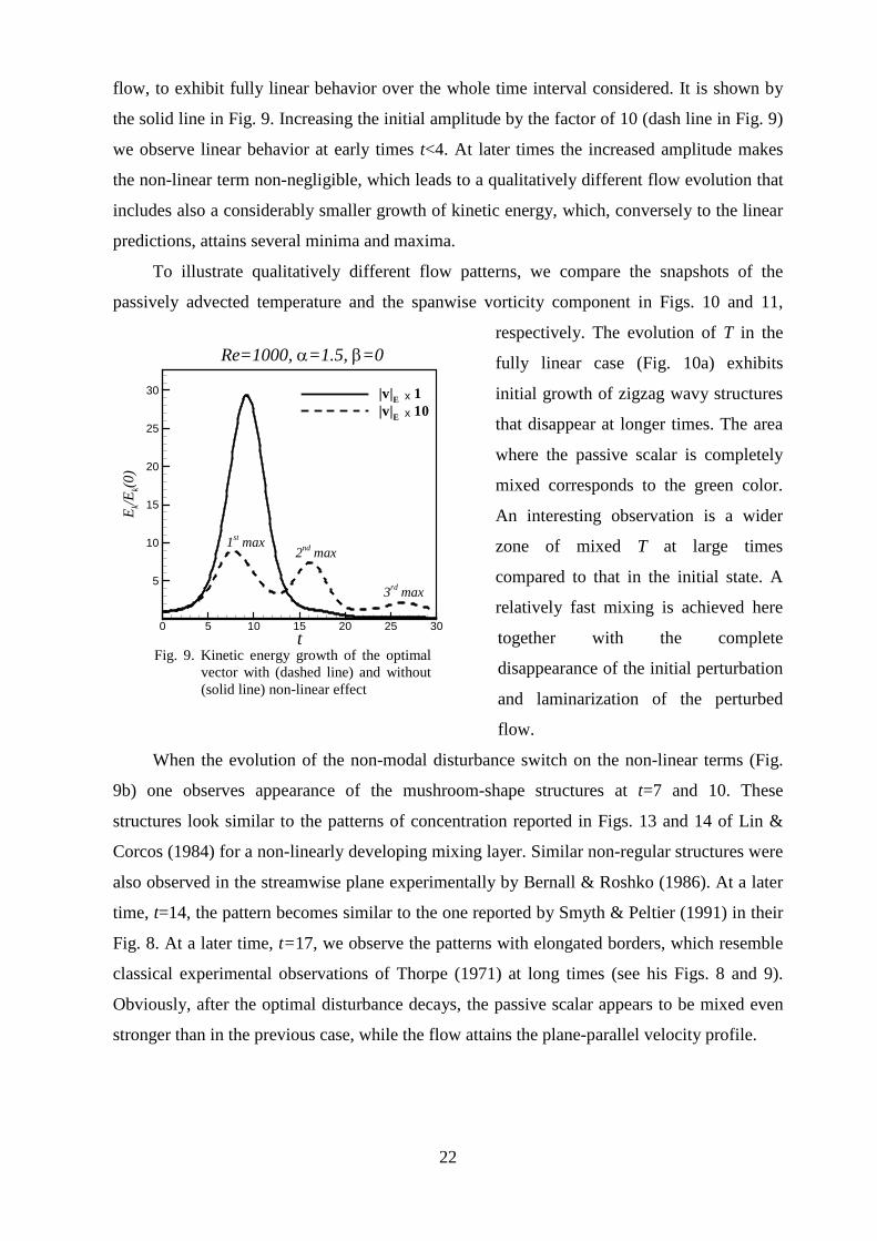
Fig. 9. Kinetic energy growth of the optimal vector with (dashed line) and without (solid line) non-linear effect

flow, to exhibit fully linear behavior over the whole time interval considered. It is shown by

the solid line in Fig. 9. Increasing the initial amplitude by the factor of 10 (dash line in Fig. 9)

we observe linear behavior at early times t<4. At later times the increased amplitude makes

the non-linear term non-negligible, which leads to a qualitatively different flow evolution that

includes also a considerably smaller growth of kinetic energy, which, conversely to the linear

predictions, attains several minima and maxima.

To illustrate qualitatively different flow patterns, we compare the snapshots of the

passively advected temperature and the spanwise vorticity component in Figs. 10 and 11,

respectively. The evolution of T in the

fully linear case (Fig. 10a) exhibits

initial growth of zigzag wavy structures

that disappear at longer times. The area

where the passive scalar is completely

mixed corresponds to the green color.

An interesting observation is a wider

zone of mixed T at large times

compared to that in the initial state. A

relatively fast mixing is achieved here

together with the complete

disappearance of the initial perturbation

and laminarization of the perturbed

flow.

When the evolution of the non-modal disturbance switch on the non-linear terms (Fig.

9b) one observes appearance of the mushroom-shape structures at t=7 and 10. These

structures look similar to the patterns of concentration reported in Figs. 13 and 14 of Lin &

Corcos (1984) for a non-linearly developing mixing layer. Similar non-regular structures were

also observed in the streamwise plane experimentally by Bernall & Roshko (1986). At a later

time, t=14, the pattern becomes similar to the one reported by Smyth & Peltier (1991) in their

Fig. 8. At a later time, t=17, we observe the patterns with elongated borders, which resemble

classical experimental observations of Thorpe (1971) at long times (see his Figs. 8 and 9).

Obviously, after the optimal disturbance decays, the passive scalar appears to be mixed even

stronger than in the previous case, while the flow attains the plane-parallel velocity profile.

23

(a) Linear evolution

(b) Non-linear effect

Fig. 10. Snapshots of the passively advected temperature in cases of (a) linear and (b) non-linear time evolution

of the optimal disturbance. Re=1000, α=1.5, β=0. Initial amplitude in the case (b) is 10 times larger than that of the case (a).

Snapshots of the spanwise vorticity are shown in Fig. 11. At early times the vorticity

pattern consists of structures tilted against the shear slope, which we attribute to the Orr

mechanism. At a later, time we observe that vorticity patterns are rotated, apparently by the

base flow, around their centers located at the midplane. Again, we see some similarities of the

vorticity behavior with the fully non-linear results reported, e.g., by Rogers & Moser (1992)

and Smyth & Peltier (1991).

It should be noted that we are examining transient growth of optimal disturbance in

order to discover transition of a parametrically stable flow to unstable regime. To do this we

increase the amplitude of the initial optimal perturbation so non-linear terms will be triggered

at later stages of the time evolution. The present calculations show that these non-linear

effects do not lead to a noticeable sub-unstable transition. However, the optimal perturbation

evaluates by different way than a non-linear evolution of perturbation based on the most

unstable linear eigenmode, or KH mode, in unstable flow regime. As a calculation test, we

performed non-linear computations using KH mode as initial vector and observed well-known

evolution of the spanwise vortices described, e.g., in Ho & Huerre (1984). As it is seen from

24

Figure 4.2.14, the evolution of the optimal vector is governed mainly by Orr-mechanism and

differs qualitatively from the evolution of the leading linearly unstable mode.

Comparing the vorticity perturbation pattern with the change of the growth function (cf.

Figs. 9 and 11), we observe that when the kinetic energy norm reaches the minimum, the

vorticity isolines are elongated along the shear slope. At later times they turn against the

shear, which leads to the next temporal growth. The maximal values of the kinetic energy

norm correspond to the vorticity patterns elongated vertically, exactly as it was observed for

the linearized problem.

Similarities between the computed flow structures and those observed in previous

experimental and numerical studies allow us to make the following assumption. At late stages

of time-development, the actual width of the mixing layer grows, thus leading to the growth of

the dimensionless streamwise wavenumber α. This necessarily results in a stabilization of the

mixing layer flow. However, at this stage the flow is already strongly perturbed. Therefore, it

is possible that development of the mixing layer flow at late stages is governed or strongly

affected by the non-modal growth. The latter results in the flow structures similar to the ones

observed here.

Fig. 11. Snapshots of the spanwise vorticity during non-linear time evolution of the optimal disturbance.

Re=1000, α=1.5, β=0.

x

z

2 4 6 8

-2

0

2

t=6.5

x

z

2 4 6 8

-2

0

2

t=8

x

z

2 4 6 8

-2

0

2

t=15

x

z

2 4 6 8

-2

0

2

t=17

x

z

2 4 6 8

-2

0

2

t=21

x

z

2 4 6 8

-2

0

2

t=24

x

z

2 4 6 8

-2

0

2

t=27

x

z

2 4 6 8

-2

0

2

t=30

x

z

2 4 6 8

-2

0

2

t=35

x

z

2 4 6 8

-2

0

2

t=0

x

z

2 4 6 8

-2

0

2

t=25

x

z

2 4 6 8

-2

0

2

t=13

2nd max 2nd min

3rd max 3rd min

1st max 1st min

25

Fig. 12. Kinetic energy growth of a 3D optimal vector with and without non-linear effect

Time dependence of the kinetic

energy norm for the 3D optimal

disturbance is shown in Fig. 12. Similarly

to the 2D case, the disturbance having the

unity kinetic energy norm exhibits a

completely linear behavior, and non-

linear mechanisms switch on when the

amplitude is increased by the factor of 10.

However, in the 3D case the maximal

growth of kinetic energy is attained at a

considerably longer time (cf. Figs. 5 and

12), as is predicted by the above non-

modal analysis. Note that in the 3D case,

we do not observe several maxima and minima in the kinetic energy time history. Time

evolution of the passively advected temperature is shown in Fig. 13. It generally resembles the

structures observed in the 2D case, however the whole pattern is aligned along the disturbance

vector (2𝜋 𝛼⁄ , 2𝜋 𝛽⁄ ). After the perturbation decays, the width of mixed temperature zone is

even larger than that observed in the 2D case. The qualitative difference of the 2D and 3D

non-modal growth can be seen by comparison of Figs. 11 and 14. Figure 14 shows the

snapshots of spanwise vorticity in the spanwise midplane. Similarly to the 2D case, the 3D

growth starts from the optimal perturbation aligned against the shear slope. However, when

the perturbation becomes aligned along the shear (t≥20 in Fig. 14), the kinetic energy

continues to grow, thus leading to a larger growth at a longer time. This phenomenon seems to

be common for all plane parallel shear flows and is addressed in a companion paper by

Vitoshkin et al. (2013).

t

E k/Ek(0

)

0 10 20 30 40

200

400

600

800

1000 |v|E x 1|v|E x 10

Re=1000, α=0.7, β=0.8

xx

26

Fig. 13. Snapshots of the passively advected temperature during non-linear time evolution of a 3D optimal

disturbance. Re=1000, α=0.7, β=0.8.

27

Fig. 14. Snapshots of the spanwise vorticity in the spanwise midplane during non-linear time evolution of the optimal disturbance. Re=1000, α=0.7, β=0.8.

t=0 t=10

t=15 t=20

t=25 t=30

0 5 10 15 x

4.5 3

1.5 z 0 -1.5

-3 -4.5

4.5 3

1.5 z 0 -1.5

-3 -4.5

4.5 3

1.5 z 0 -1.5

-3 -4.5

4.5 3

1.5 z 0 -1.5

-3 -4.5

4.5 3

1.5 z 0 -1.5

-3 -4.5

4.5 3

1.5 z 0 -1.5

-3 -4.5

0 5 10 15 x

0 5 10 15 x

0 5 10 15 x

0 5 10 15 x

0 5 10 15 x

28

6. Conclusions

In the current study the transient perturbation dynamics in isothermal viscous mixing

layers was investigated. The research combined fundamental theoretical principles along with

the computational modelling.

The flow of interest exhibits significant transient growth, typically with many orders

of magnitude of streamwise and spanwise wavenumbers, for which the flow is asymptotically

stable. Comparing the calculated flow structures with those observed in several previous

experimental and numerical studies, we speculate that the mixing layer flow at late stages of

the linear instability development can be strongly affected by the non-modal disturbances

growth. The optimal perturbation is always localized inside the shear zone.

The following conclusions were drawn from the investigation of transient growth in an

isothermal viscous mixing layer:

• A series of numerical tests performed revealed that the mixing layer flow appears to be

a more numerically challenging problem for the non-modal growth analysis than the

problems considering bounded (e.g., plane Couette and Poiseuille flows) or semi-

inbounded (e.g., Blasius boundary layer profile) flows. The correct numerical

modeling of the non-modal growth for the 𝑡𝑎𝑛ℎ-velocity profile requires much better

resolution in the cross-flow direction than other plane-parallel flows.

• A problem that may need attention is the separation of the discrete and continuous

parts of the spectrum. We provided several arguments on why and how the discrete

modes can be extracted and why only a discrete part of the spectrum should be taken

into account when non-modal growth of disturbances in the isothermal mixing layer

flow is studied. The corresponding results are verified by using three independent

approaches for calculation of the growth function, as well as by the time-dependent

calculations applied to both the ODE system resulting from the discretized Orr-

Sommerfeld and Squire equations, and by the fully 3D non-linear time-dependent flow

model.

• There is a possibility to obtain a significant mixing without making the flow turbulent.

This observation is based on the advection of passive temperature and is observed

during both 2D and 3D, linear and non-linear evolution of an optimally disturbed

mixing layer flow. Therefore, the growth of small perturbations due to non-modal

instability consequently may provide an additional possibility for mixing.

• A three-dimensional direct numerical simulation of the mixing layer flow which starts

from the optimally perturbed base flow was conducted to investigate non-linear

29

evolution of optimal perturbation and possibility for a by-pass transition. Following

time non-linear evolution of the optimal disturbances, we observe qualitatively

different development in 2D and 3D cases. In the 2D case, the non-linear effects lead

to the appearance of several maxima and minima in the time history of the kinetic

energy. Evolution of the spanwise vorticity pattern reveals that the minima are

observed when the iso-vorticity lines are tilted along the shear slope. The temporal

growth starts when the isolines become tilted against the shear, and the maxima are

reached when they are rotated by the base flow until they become vertically aligned.

No several minima or maxima are observed in the non-linear development of the 3D

optimal disturbances. The maximum of the kinetic energy in the 3D case is attained

significantly later, compared to the 2D case, after the patterns had turned in the base

flow direction.

Acknowledgement

This study was supported by BSF (Bi-National US-Israeli Foundation) grant No. 2004087.

The authors wish to express their thankfulness to E. Kit and E. Heifez for long and fruitful

discussions of these results.

30

REFERENCES Åkervik E., Ehrenstein U., Gallaire F., and Henningson D.S. 2008 Global two-dimensional

stability measures on the flat plate boundary-later flow. Eur. J. Mech. B/Fluids, 27, 501-513.

Andersson P., Berggren M., and Henningson D.S. 1999 Optimal disturbances and bypass transition in boundary layers, Phys. Fluids, 11, 134-150.

Bakas N.A. and Ioannou P.J. 2009 Modal and nonmodal growths of inviscid planar perturbations in shear flows with a free surface. Phys. Fluids, 21, 024102.

Bernal L.P. and Roshko A. 1986 Streamwise vortex structure in plane mixing layers. J. Fluid Mech., 170, 499-525.

Bun Y. and Criminale W.O. 1994 Early-period dynamics of an incompressible mixing layer. J. Fluid Mech., 273, 21-82.

Butler R.M. and Farrell B.F. 1992 Three-dimensional optimal perturbations in viscous shear flows, Phys. Fluids A, 4, 1367-1650.

Corbett P. and Bottaro A. 2000 Optimal perturbations for boundary layers subject to stream-wise pressure gradient. Phys. Fluids, 12, 120-130.

Criminale W.O., Jackson T.L. and Lasseigne D. 1995 Towards enhancing and delaying disturbances in free shear flows, J. Fluid Mech., 294, 283-300.

Criminale W.O., Jakson T.L. and Joslin R.D. 2003 Theory and computation in Hydrodynamic Stability. Cambridge University Press.

Farrell B.F. 1987 Developing disturbances in shear. J. Atmospheric Sci., 44, 2191-2199.

Farrell B.F. 1988. Optimal excitation of perturbations in viscous shear flow. Phys. Fluids, 31, 2093-2102.

Gaster M., Kit E., and Wygnanski I. 1985 Large-Scale Structures in a Forced Turbulent Mixing Layer. J. Fluid Mech., 150, 23-39.

Gelfgat A.Yu. and Kit E. 2006 Spatial versus temporal instabilities in a parametrically forced stratified mixing layer, J. Fluid Mech., 552, 189-227.

Grosch C.E. and Salwen H. 1978 The continuous spectrum of the Orr-Sommerfeld equation. Part 1. The spectrum and the eigenfunctions. J. Fluid Mech., 87, 33-54.

Hazel P. 1972 Numerical studies of the stability of inviscid stratified shear flows. . J. Fluid Mech., 51, 39-61.

Healey J. J. 2009 Destabilizing effects of confinement on homogeneous mixing layers. J. Fluid Mech., 623, 241–271.

Heifetz E. and Methven J. 2005 Relating optimal growth to counterpropagating Rossby wavesin shear instability. Phys. Fluids, 17, 064107.

Ho C.-M., Huerre P. Perturbed free shear layers. Ann. Rev. Fluid Mech., 16, 365–424, 1984.

Joseph D.D. 1976. Stability of Fluid Motions. Springer-Verlag, New York.

Kit E., Wygnansky I., Friedman D., Krivonosova O., and Zhilenko D. 2007 On the periodically excited plane turbulent mixing layer, emanating from a jagged partition. J. Fluid Mech., 589, 479-507.

31

Kit E., Gerstenfeld D., Gelfgat A. Y., and Nikitin N.V. 2010 Bulging and bending of Kelvin-Helmholtz billows controlled by symmetry and phase of initial perturbation. J. Physics: Conference Series, 216, 012019.

Le Dizès S. 2003 Modal growth and non-modal growth in a stretched shear layer. Eur. J. Mech., B/Fluids, 22, 411-430.

Lin S.J. and Corcos G.M. 1984 The mixing layer: deterministic models of a turbulent flow. Part 3. The effect of plane strain on the dynamics of streamwise vortices. J. Fluid Mech., 141, 139-178.

Mao X. and Sherwin S. J. 2012 Transient growth associated with continuous spectra of the Batchelor vortex. J. Fluid Mech., 697, 35-59.

Reddy S.C. and Henningson D.S. 1993 Energy growth in viscous channel flows, J. Fluid Mech., 252, 209-238.

Rogers M. M. and Moser R. D. 1992 The three-dimensional evolution of a plane mixing layer: the Kelvin-Helmholtz rollup. J. Fluid Mech., 243, 183-226.

Schmid P.J. 2000 Linear stability theory and bypass transition in shear flows. Physics of Plasmas, 7, 1788-1794.

Schmid P.J. and Henningson D.S. Stability and transition in shear flows. Springer, N.Y., 2001.

Smyth W.D. and Peltier W.R. 1991 Instability and transition in finite-amplitude Kelvin-Helmhotz and Holmboe waves. J. Fluid Mech., 228, 387-415.

Thorpe S.A. 1971 Experiments on the instability of stratified shear flows: miscible fluids. J. Fluid Mech., 46, 299-319.

Trefethen L. N. and Embree M. 2005 Spectra and Pseudospectra: The Behavior of Nonnormal Matrices and Operators. Princeton University Press, 624 pp.

Vitoshkin H., and Gelfgat A. Y. 2013 On direct inverse of Stokes, Helmholtz and Laplacian operators in view of time-stepper-based Newton and Arnoldi solvers in incompressible CFD. Submitted for publication. arXiv:1107.2461v1

Vitoshkin H., Heifetz E., Gelfgat A. Y., Harnik N. 2013 On the role of vorticity stretching in optimal growth of three dimensional perturbations on plane parallel shear flows. J. Fluid Mech., 707, 369-380.

Yecko P., Zaleski S., and Fullana J.-M. 2002 Viscous modes in two-phase mixing layers. Phys. Fluids, 14, 4115-4123.

Yecko P. and Zaleski S. 2005 Transient growth in two-phase mixing layers. J. Fluid Mech., 528, 43-52.

32

APPENDIX A – Estimation of the effect of viscous dissipation effect on the

plane-parallel mixing layer flow

The linearized Orr-Sommerfeld and Squire equations assume that the plane-parallel

mixing layer flow is frozen. This is correct only within the inviscid flow model. In the

viscous case the tanh-mixing layer width is continuously growing, which is most profound at

small Reynolds numbers, i.e., at large viscosities. In the following, we present a simple model

allowing us to estimate until which times the viscosity effect can be neglected.

Consider the unsteady momentum equation with initial velocity u(0,0,u(t,z)), where

u(t=0,z) has the hyperbolic tangent profile. We want to estimate how the mixing layer

thickness δv varies, owing to viscosity, with time at different Reynolds numbers. Assuming

that the flow remains pane-parallel, we arrive at a problem similar to the one dimensional heat

conduction equation: 𝜕𝑢𝜕𝑡

= 1𝑅𝑒

𝜕2𝑢𝜕𝑧2

, (A.1)

𝑢(𝑡 = 0) = 𝑡𝑎𝑛ℎ(𝑧) ,𝑢(𝐿) = 1,𝑢(−𝐿) = −1, (A.2)

The solution of (A.1)-(A.2) is obtained by the standard separation of variables

𝑢(𝑡, 𝑧) = 1 +𝑧 + 𝐿𝐿

+2𝜋�

cos(𝑛𝜋) + 1𝑛

sin𝑛𝜋(𝑧 + 𝐿)

2𝐿𝑒−

𝑛2𝜋2𝑡4𝐿2𝑅𝑒

∞

1

+ 1𝐿∑ ∫ �tanh(ξ − L) sin 𝑛𝜋𝜉

2𝐿� 𝑑𝜉2L

0 sin 𝑛𝜋(𝑧+𝐿)2𝐿

𝑒−𝑛2𝜋2𝑡4𝐿2𝑅𝑒∞

1 , (A.3)

The shear layer thickness is defined as a distance between the points at which the velocity

attains the values of ±0.99. The result is presented in Figure A1. Obviously, for Re≤10 the

layer thickness strongly depends on the

Reynolds number. For 10≤Re≤100 the

linearized problem is meaningful only at

very short times, t<2, however, it already

allows considering the linear stability of the

flow. For Re>100 the thickness remains

almost unchanged until t=30. Note that the

reported maximal values of the non-modal

growth functions were reached within this

time interval.

Re

δ v/2

100 101 102 103

5

10

15

20t=30

t=20

t=10

t=5

t=2t=1t=0

Fig. A1. Values of the shear layer thickness as a function of the Reynolds number and time.

33

APPENDIX B – Eigenproblem and complex conjugated eigenvalues

Consider the eigenproblem related to equations (2) and (3). Assuming 𝑤(𝑧, 𝑡) =

𝑤(𝑧)𝑒𝜆𝑡, 𝜂(𝑧, 𝑡) = 𝜂(𝑧)𝑒𝜆𝑡 we obtain

λ(𝑤′′ − 𝑘2𝑤) = 𝑖𝛼[𝑈′′𝑤 − 𝑈(𝑤′′ − 𝑘2𝑤)] − 1𝑅𝑒

(𝑤′′′′ − 2𝑘2𝑤′′ + 𝑘4𝑤), (B.1)

𝜆𝜂 = −𝑖𝛽𝑈′𝑤 + 1𝑅𝑒

(𝜂′′ − 𝑘2𝜂) − 𝑖𝛼𝑈𝜂, (B.2)

where the tag denotes the derivative with respect to z. Assume also that 𝜆 = 𝜆𝑟 + 𝑖𝜆𝑖 is an

eigenvalue, and 𝑤(𝑧) = 𝑤𝑟(𝑧) + 𝑖𝑤𝑖(𝑧), 𝜂(𝑧) = 𝜂𝑟(𝑧) + 𝑖𝜂𝑖(𝑧) are the corresponding

eigenfunctions of (B.1, B.2). Substituting these expressions back into equations (B.1), (B.2)

and separating real and imaginary parts yields the two following pairs of equations:

𝜆𝑟(𝑤𝑟′′ − 𝑘2𝑤𝑟) − 𝜆𝑖(𝑤𝑖′′ − 𝑘2𝑤𝑖) =

= −𝛼[𝑈′′𝑤𝑖 − 𝑈(𝑤𝑖′′ − 𝑘2𝑤𝑖)] − 1

𝑅𝑒(𝑤𝑟′′′′ − 2𝑘2𝑤𝑟′′ + 𝑘4𝑤𝑟) (B.3)

𝜆𝑖(𝑤𝑟′′ − 𝑘2𝑤𝑟) + 𝜆𝑟(𝑤𝑖′′ − 𝑘2𝑤𝑖) =

= 𝛼[𝑈′′𝑤𝑟 − 𝑈(𝑤𝑟′′ − 𝑘2𝑤𝑟)]− 1𝑅𝑒

(𝑤𝑖′′′′ − 2𝑘2𝑤𝑖

′′ + 𝑘4𝑤𝑖) (B.4)

𝜆𝑟𝜂𝑟 − 𝜆𝑖𝜂𝑖 = 𝛽𝑈′𝑤𝑖 + 1𝑅𝑒

(𝜂𝑟′′ − 𝑘2𝜂𝑟) + 𝛼𝑈𝜂𝑖 (B.5)

𝜆𝑟𝜂𝑖 + 𝜆𝑖𝜂𝑟 = −𝛽𝑈′𝑤𝑟 + 1𝑅𝑒

(𝜂𝑖′′ − 𝑘2𝜂𝑖) − 𝛼𝑈𝜂𝑟 (B.6)

We notice that due to the fact that tanh(z) is an odd function of z, the transformation

𝑧 → −𝑧, 𝑈(𝑧) = −𝑈(−𝑧) results in the same problem. Applying this transformation to

equations (B.3)-(B.6) yields

�̂�𝑟(𝑤�𝑟′′ − 𝑘2𝑤�𝑟) − �̂�𝑖(𝑤�𝑖′′ − 𝑘2𝑤�𝑖) =

= 𝛼[𝑈′′𝑤�𝑖 − 𝑈(𝑤�𝑖′′ − 𝑘2𝑤�𝑖)] − 1𝑅𝑒

(𝑤�𝑟′′′′ − 2𝑘2𝑤�𝑟′′ + 𝑘4𝑤�𝑟) (B.7)

𝜆𝑖(𝑤�𝑟′′ − 𝑘2𝑤�𝑟) + 𝜆𝑟(𝑤�𝑖′′ − 𝑘2𝑤�𝑖) =

= −𝛼[𝑈′′𝑤�𝑟 − 𝑈(𝑤�𝑟′′ − 𝑘2𝑤�𝑟)]− 1𝑅𝑒

(𝑤�𝑖′′′′ − 2𝑘2𝑤�𝑖′′ + 𝑘4𝑤�𝑖) (B.8)

𝜆𝑟�̂�𝑟 − 𝜆𝑖�̂�𝑖 = −𝛽𝑈′𝑤�𝑖 + 1𝑅𝑒

(�̂�𝑟′′ − 𝑘2�̂�𝑟) − 𝛼𝑈�̂�𝑖 (B.9)

𝜆𝑟�̂�𝑖 + 𝜆𝑖�̂�𝑟 = 𝛽𝑈′𝑤�𝑟 + 1𝑅𝑒

(�̂�𝑖′′ − 𝑘2�̂�𝑖) + 𝛼𝑈�̂�𝑟 (B.10)

where all the functions depend on (−𝑧). The problems (B.3)-(B.6) and (B.7)-(B.10) are

identical and have the same solutions. It is easy to see that choosing �̂�𝑟 = 𝜆𝑟, �̂�𝑖 = −𝜆𝑖,

𝑤�𝑟(−𝑧) = 𝑤𝑟(𝑧), 𝑤�𝑖(−𝑧) = −𝑤𝑖(𝑧), �̂�𝑟(−𝑧) = 𝜂𝑟(𝑧), �̂�𝑖(−𝑧) = −𝜂𝑖(𝑧), we arrive to the

equations (B.3)-(B.6). Thus, if 𝜆 = 𝜆𝑟 + 𝑖𝜆𝑖 is the eigenvalue of (B.1), (B.2), then 𝜆 = 𝜆𝑟 −

𝑖𝜆𝑖 is also the eigenvalue. The corresponding eigenvectors are connected via reflection and

antireflection of their real and imaginary parts, respectively, with respect to the plane z=0.

34

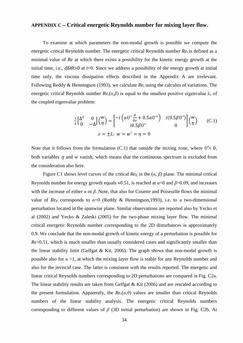
APPENDIX C – Critical energetic Reynolds number for mixing layer flow.

To examine at which parameters the non-modal growth is possible we compute the

energetic critical Reynolds number. The energetic critical Reynolds number ReE is defined as a

minimal value of Re at which there exists a possibility for the kinetic energy growth at the

initial time, i.e., dE⁄dt>0 at t=0. Since we address a possibility of the energy growth at initial

time only, the viscous dissipation effects described in the Appendix A are irrelevant.

Following Reddy & Henningson (1993), we calculate ReE using the calculus of variations. The

energetic critical Reynolds number ReE(α,β) is equal to the smallest positive eigenvalue λ, of

the coupled eigenvalue problem:

1𝜆�∆

2 00 −∆

� �𝑤𝜂� = �−𝑖 �𝛼𝑈

′ 𝜕𝜕𝑧

+ 0.5𝛼𝑈′′� 𝑖(0.5𝛽𝑈′)𝑖0.5𝛽𝑈′ 0

� �𝑤𝜂� (C.1)

𝑧 = ±𝐿: 𝑤 = 𝑤′ = 𝜂 = 0

Note that it follows from the formulation (C.1) that outside the mixing zone, where U'= 0,

both variables η and w vanish, which means that the continuous spectrum is excluded from

the consideration also here.

Figure C1 shows level curves of the critical ReE in the (α, β) plane. The minimal critical

Reynolds number for energy growth equals ≈0.51, is reached at α=0 and β=0.09, and increases

with the increase of either α or β. Note, that also for Couette and Poiseuille flows the minimal

value of ReE corresponds to α=0 (Reddy & Henningson,1993), i.e. to a two-dimensional

perturbation located in the spanwise plane. Similar observations are reported also by Yecko et

al (2002) and Yecko & Zaleski (2005) for the two-phase mixing layer flow. The minimal

critical energetic Reynolds number corresponding to the 2D disturbances is approximately

0.9. We conclude that the non-modal growth of kinetic energy of a perturbation is possible for

Re>0.51, which is much smaller than usually considered cases and significantly smaller than

the linear stability limit (Gelfgat & Kit, 2006). The graph shows that non-modal growth is

possible also for α >1, at which the mixing layer flow is stable for any Reynolds number and

also for the inviscid case. The latter is consistent with the results reported. The energetic and

linear critical Reynolds numbers corresponding to 2D perturbations are compared in Fig. C2a.

The linear stability results are taken from Gelfgat & Kit (2006) and are rescaled according to

the present formulation. Apparently, the ReE(α,0) values are smaller than critical Reynolds

numbers of the linear stability analysis. The energetic critical Reynolds numbers

corresponding to different values of β (3D initial perturbation) are shown in Fig. C2b. At

35

small, but non-zero, values of β the three-dimensional perturbations exhibit earlier initial

growth than the two-dimensional ones corresponding to β=0. With the increase of β the curves

corresponding to different β tend to coincide. This means that at the same value of α the initial

growth can start as a superposition of several initial perturbations having different spanwise

periodicity. This can be important for understanding experimental results, as well as for

choice of the computational domain and initial states for computational simulations.

Fig. C1. Level curves of ReE(α,β) for mixing layer flow. Frame (b) zooms in the lower left corner of frame (a).

Fig. C2. (a) Critical linear and an energetic stability curves for two-dimensional disturbances (β=0). (b) Critical energetic Reynolds numbers ReE as functions of α and β.

6 9

9

12

12

15

15

18

18

21

α

β

0 0.5 1 1.5 20

0.5

1

1.5

2

(a)

0.6

0.8

0.8

1.0

1.0

1.0

1.5

1.5

2.0

2.0

2.5

2.5

3.0

3.0

3.5

3.5

α

β0 0.1 0.2 0.3 0.4 0.50

0.1

0.2

0.3

(b)

Re

α

100 101 1020

0.5

1

1.5

ReLReE

(a)

ReE

α

0 5 10 15 20 250

0.5

1

1.5

β=0β=0.05β=0.1β=0.2β=0.3β=1β=2

(b)

ReE

α

0.5 0.75 10

0.05

0.1

0.15