Non-Minimum Phase Surface Consistent Sparsity Constrained Blind DeconvolutionNasser Kazemi*, Emmanuel Bongajum , and Mauricio D. Sacchi, Department of Physics, University of Alberta

SUMMARY

We describe a method that allows for blind surface consistentestimation of the source and receiver wavelets. This is very rel-evant for surface consistent deconvolution where current pro-cessing standards focus on the removal of the source and re-ceiver effects under the minimum phase assumption. The pro-posed method, which is an extension of the Euclid deconvo-lution method, employs an iterative algorithm that simultane-ously estimates the source-receiver wavelets that are consistentwith the data. Unlike most deconvolution methods the algo-rithm requires no prior phase assumptions.

INTRODUCTION

Land seismic data suffers from near surface effects. Lateralvariations in near surface heterogeneity contribute towards thevariations in the reflection amplitudes as well as time delays.These distortions in the seismic record can be primarily viewedas a compound effect of the heterogeneous environment in thevicinity of the source and receiver locations. Consequently,surface consistent deconvolution (SCD) has been commonlyused for processing of land seismic data in order to estimateand remove source and receiver effects. Contrary to single-trace deconvolution methods, SCD is a multichannel decon-volution approach. Various types of SCD methods exist, witheach using different assumptions and decompositions of theseismic traces in order to take advantage of data redundancy(Taner and Koehler, 1981). While some decompositions usemidpoint binning (Taner and Koehler, 1981) others use reci-procity of the medium response (Vossen et al., 2006). SCD canbe performed in the log/Fourier domain (Taner and Koehler,1981; Morley and Claerbout, 1983; Cambois and Stoffa, 1992;Cary and Lorentz, 1993; Vossen et al., 2006) or in the time do-main (Levin, 1989). Levin (1989) also argues that the validityof the surface consistent decomposition model that is adoptedis very important in order to obtain more stable and correct es-timates of the individual deconvolution operators. When SCDis performed in the log/Fourier domain, the problem becomeslinear with respect to the amplitude spectrum of source and re-ceiver components. The log/Fourier domain allows for the sep-aration of the amplitude spectrum of each component. How-ever, SCD in the log/Fourier domain does not have control onphase estimation and the minimum phase assumption must beinvoked.

Most authors have focused on the surface consistent decom-position of the spectral amplitudes (Taner and Koehler, 1981;Morley and Claerbout, 1983; Cambois and Stoffa, 1992; Caryand Lorentz, 1993; Vossen et al., 2006) where the minimumphase assumption is usually used. A comprehensive SCD ap-proach warrants the correct estimation of the amplitude andphase information of the individual deconvolution operators.Unfortunately, very little focus has been directed at the surfaceconsistent decomposition of the phase spectra (Cambois and

Stoffa, 1992).

Our work expands the Euclid deconvolution (Rietsch, 1997;Xu et al., 1995; Mazzucchelli and Spagnolini, 2001) to thecase of SCD. In other words, the homogeneous system of equa-tions arising in Euclid deconvolution is reformulated in termsof SCD and an alternating optimization algorithm is proposedto estimate source and receiver wavelets. The estimated opera-tors in turn permit the computation of inverse filters to equalizethe pre-stack volume.

THEORYIn order to explain the surface consistent extension of the Eu-clid deconvolution, let us consider a simple acquisition geom-etry containing two shots (i.e., i and j) and two receivers (i.e.,m and n). The z-transform of the noise-free seismic trace dimcreated by source i and recorded by receiver m can be writtenas

Dim(z) = Si(z)Gm(z)Rim(z) (1)

where Si(z), Gm(z), Rim(z) represent the z-transform of thesource function, the receiver response, and the medium re-sponse respectively. Following the decomposition model in(1), one can also write the z-transform of another trace withinsame shot gather as

Din(z) = Si(z)Gn(z)Rin(z). (2)

Dividing (1) by (2) leads to

Din(z)Gm(z)Rim(z)−Dim(z)Gn(z)Rin(z) = 0. (3)

Similar steps can be used for trace pairs from a common source(s j) and common receivers (gm,gn) to obtain

D jn(z)Gm(z)R jm(z)−D jm(z)Gn(z)R jn(z) = 0. (4)

D jm(z)Si(z)Rim(z)−Dim(z)S j(z)R jm(z) = 0. (5)

D jn(z)Si(z)Rin(z)−Din(z)S j(z)R jn(z) = 0. (6)

Equations (3) to (6) form a homogeneous system of equations.This system of equations can be written in matrix notation asfollows

DinGm −DimGn 0 00 0 D jnGm −D jmGn

D jmSi 0 −DimS j 00 D jnSi 0 −DinS j

rimrinr jmr jn

= 0

(7)where rim is a column vector representing the correspondingreflectivity for the source-receiver pair (si,gm). Similarly, Din,Gm, and Si correspond to convolution matrices derived fromDin(z), Gm(z), and Si(z) respectively. For a data set with NSshots (NS ≥ 3) and NG receivers (NG ≥ 3), the maximumnumber of trace combinations that can be used to derive the ho-mogeneous system of equations is 0.5×NS×NG(NG+NS−2).If one uses all the combinations, equation (7) can be expressedas follows

Ar = 0 (8)

Blind SCD

where r contains all media responses organized in a single col-umn vector. We propose to estimate the source and receivercomponents by minimizing a cost function J given by

J = ‖Ar‖22 +µR(r) , subject to‖r‖2

2 = 1 (9)

where the constraint ‖r‖22 = 1 is needed to avoid the trivial so-

lution r = 0 and R(r) is a sparsity promoting regularizationterm. In our tests we have explored different norms that pro-mote sparsity and have finally adopted the hyperbolic normproposed by Bube and Langan (1997). The cost function Jdepends not only on the unknown reflectivity sequences butalso on source wavelets si, i = 1 . . .NS and receiver waveletsgi, i = 1 . . .NG. Therefore, the cost function J must be opti-mized via an alternating algorithm that estimates all unknownsvia the following iterative scheme

“r-step” : r = argminr

[J] subject to ‖r‖22 = 1 (10)

“s-step” : si = argmins

[J ], i = 1 . . .NS (11)

“g-step” : gm = argming

[J ], m = 1 . . .NG (12)

Note that equation (10) is similar to the method proposed byNojadeh and Sacchi (2013) for multichannel blind deconvo-lution. Equation (10) is solved via an iterative algorithm thatassumes the source and receiver wavelets are known. Then, thereflectivity estimates from equation (10) are used to computethe source and receiver wavelets by solving the problems givenby equations (11) and (12). It is easy to show that the steps “s”and “g” of the algorithm are equivalent to solving a surfaceconsistent least squares problem for estimating the source andreceiver operators, respectively. In matrix notation we have

“s-step” :

si = argminsi

{NG∑p=1||B(gp,rip)si−dip||22

}, i = 1 . . .NS

(13)

“g-step” :

gm = argmingm

{NS∑

k=1||C(sk,rkm)gm−dkm||22

}, m = 1 . . .NG

(14)where B(gp,rip) and C(sk,rkm) represent convolution matri-ces derived from Gp(z)Rip(z) and Sk(z)Rkm(z) respectively.Consequently, we use equations (13) and (14) to simplify andspeed up the iterative algorithm. These equations are eas-ily solved via a multichannel frequency domain Wiener fil-ter. In essence, our algorithm starts with initial source andreceiver wavelets to estimate r via equation (10), then eachsource wavelet and each receiver wavelet is updated in turn,via equations (13) and (14) using the current estimates of allthe other sources, receivers and r.

EXAMPLE

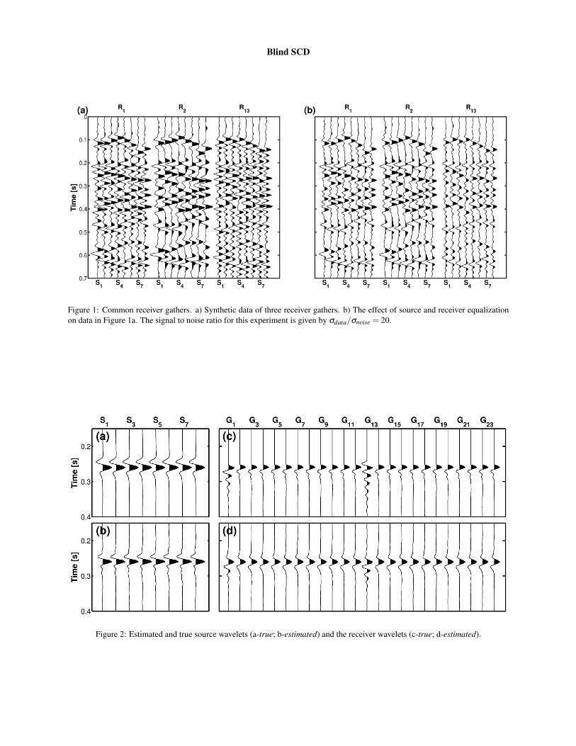
To evaluate the viability of the method we generated a syn-thetic data set consisting of eight shot gathers. The synthetic

traces were obtained by convolving the source wavelets, withthe receiver wavelets and sparse reflectivity series. All shotgathers are generated with identical sets of twenty-four re-ceiver wavelets. Receivers 1 and 13 have been perturbed to in-clude ringing responses. All wavelets are non-minimum phase.Figure 1a shows a sample of the subset of receiver gathers.Figure 1b shows the data after the source and receiver effectshave been deconvolved. The quality of the blind surface con-sistent wavelet estimates used for the deconvolution is shownin Figure 2. In the inversion process, the wavelets are assumedto be stationary throughout the time domain of the input data.The algorithm does a reasonable job in estimating the sourceand receiver wavelets for each trace in the data.

Next, we applied the method on 2D land data set from AlaskaNorth Slope. To analyze the performance of the proposedmethod in estimating the source and receiver wavelets, we se-lected nine consecutive shot gathers (Figure 3a). Figure 3bshows the estimated source wavelets. Figure 3c shows the es-timated receiver wavelets that are shared with all nine shotgathers. To evaluate the differences in the estimated sourcewavelets, we applied phase rotation to the wavelets in a waythat it maximizes the kurtosis of the source wavelets. The re-sults are shown in Figure 3d. The algorithm was also applied tothe whole data set. Figure 4a shows the common offset sectionof the data set (i.e., 2255m). Figure 4b represents the sectionafter the source and receiver effects have been removed by theproposed method. Finally, Figure 4c is the estimated sparsereflectivity series of the common offset section. We are not ad-vocating using the sparse reflectivity derived in this manner fordata interpretation. Our ultimate goal is to use the sparse re-flectivity assumption to improve the estimation of surface con-sistent deconvolution operators and to guarantee a zero phasevolume that is consistent across sources and receivers. Once,the data has been properly equalized via surface consistentdeconvolution, the stack could be enhanced via sparse singlechannel deconvolution or by any tool that aims at increasingbandwidth to facilitate seismic interpretation (Chopra et al.,2006). It is worth mentioning that, at this point our method issensitive to ground roll and erratic noise. Hence, we appliedthe algorithm on the data set after suppressing ground roll anderratic noise.

CONCLUSIONAn important step in the processing of land seismic data in-volves performing surface consistent deconvolution. We havedescribed a surface consistent method that estimates the sourceand receiver wavelets which can then be used to deconvolvethe data. Unlike other existing SCD methods, no assump-tions about the phase of the source and receiver componentsare made. We impose sparsity constraints on the reflectivitysequence in order to circumvent the minimum phase assump-tion.

AcknowledgementsWe are grateful to the sponsors of the Signal Analysis andImaging Group (SAIG) at the University of Alberta. We alsothank the USGS for the real data example and the SEG forfacilitating access to the data via http://wiki.seg.org.

Blind SCD

Figure 1: Common receiver gathers. a) Synthetic data of three receiver gathers. b) The effect of source and receiver equalizationon data in Figure 1a. The signal to noise ratio for this experiment is given by σdata/σnoise = 20.

Figure 2: Estimated and true source wavelets (a-true; b-estimated) and the receiver wavelets (c-true; d-estimated).

Blind SCD

(a) (b)

(c) (d)

0

0.5

1.0

1.5

2.0

2.5

3.0

Tim

e (s

)Shot gathers

0

0.1

0.2

Tim

e (s

)

1 2 3 4 5 6 7 8 9Source Wavelets

0

0.1

0.2

Tim

e (s

)

10 20 30 40 50 60Receiver Wavelets

2 3 4 5 6 7 8 9

20

25

30

35

40

45

Shot number

Pha

se (

degr

ee)

Figure 3: Performance of the method in estimating the source and the receivers wavelets. a) Nine consecutive shot gathers fromAlaska North Slop data set. b) Estimated source wavelets. c) Estimated receiver wavelets. d) Estimation of the phase of the sourcewavelets via maximizing the kurtosis of the wavelets.

0.6

0.8

1.0

1.2

1.4

1.6

1.8

Tim

e (s

)

10 20 30 40 50Shot number(a)

0.6

0.8

1.0

1.2

1.4

1.6

1.8

Tim

e (s

)

10 20 30 40 50Shot number(b)

0.6

0.8

1.0

1.2

1.4

1.6

1.8

Tim

e (s

)

10 20 30 40 50Shot number(c)

Figure 4: Common offset section of the Alaska North Slope data set. a) Before application of the proposed method. b) Afterdeconvolving the effects of source and receiver wavelets. c) Estimated sparse reflectivity series using the proposed method.

Blind SCD

REFERENCES

Bube, K., and R. Langan, 1997, Hybrid minimization with applications to tomography: Geophysics, 62, 1183–1195.Cambois, G., and P. Stoffa, 1992, Surface-consistent deconvolution in the log/fourier domain: Geophysics, 57, 823–840.Cary, P., and G. Lorentz, 1993, Four component surface-consistent deconvolution: Geophysics, 58, 383–392.Chopra, S., J. Castagna, and O. Portniaguine, 2006, Seismic resolution and thin-bed reflectivity inversion: CSEG recorder, 31,

19–25.Levin, S., 1989, Surface consistent deconvolution: Geophysics, 54, 1123–1133.Mazzucchelli, P., and U. Spagnolini, 2001, Least squares multichannel deconvolution: EAGE 63rd Conference and Technical

Exhibition.Morley, L., and J. Claerbout, 1983, Predictive deconvolution in shot-receiver space: Geophysics, 48, 515–531.Nojadeh, N. K., and M. D. Sacchi, 2013, Wavelet estimation via sparse multichannel blind deconvolution: EAGE 75th Conference

and Exhibition, Extended Abstracts, Tu P12 12.Rietsch, E., 1997, Euclid and the art of wavelet estimation, part II: Robust algorithm and field-data examples: Geophysics, 62,

1939–1946.Taner, M., and F. Koehler, 1981, Surface consistent corrections: Geophysics, 46, 17–22.Vossen, R., A. Curtis, A. Laake, and J. Trampert, 2006, Surface-consistent deconvolution using reciprocity and waveform inversion:

Geophysics, 71, V19–V30.Xu, G., H. Liu, L. Tong, and T. Kailath, 1995, A least-squares approach to blind channel identification: IEEE Transactions on

Signal Processing, 43, 2982 –2993.