non linear geometric elastic analysis of thin...
TRANSCRIPT

Non Linear Geometric Elastic Analysis of Thin Walled Beam by the
Finite Strip Element Method
Master thesis
Faculté Polytechnique de Mons
Alejandro Lifante Mira
Coralie AVEZ
Supervised by :
Dr. Prof. IrSélimDatoussaïd, FacultéPolytechnique de Mons
August 2014
Faculté Polytechnique
1 | P a g e
Contents 1. Introduction............................................................................................................................... 3
1.1 Background.......................................................................................................................... 3
1.2. Objectives and scope ......................................................................................................... 3
2. Previous theories ....................................................................................................................... 5
2.1. Theoretical background ..................................................................................................... 5
2.2. Existing methods ................................................................................................................ 5
2.2.1.Exact methods .............................................................................................................. 5
2.2.2. Approximate methods ................................................................................................ 6
2.2.3. Finite element method ................................................................................................ 6
2.3. Comparative table between FSM and FEM ........................................................................ 7
3. Finite Element Method (FEM) ................................................................................................... 8
3.1. History ................................................................................................................................ 8
3.1.2. Creation of the Method .............................................................................................. 8
3.1.3. Practical use of the method through the centuries .................................................... 8
3.3. FEM example ...................................................................................................................... 9
3.3.1. Situation ...................................................................................................................... 9
3.3.2 Element solving .......................................................................................................... 10
4. Finite Strip Method (FSM) ....................................................................................................... 16
4.1. History .............................................................................................................................. 16
4.2. Explanation ....................................................................................................................... 16
4.3. The finite strip analysis ..................................................................................................... 17
4.3.1. Degree of freedom and shape functions .................................................................. 17
4.3.2. Elastic stiffness matrix ............................................................................................... 21
4.3.3. Geometric stiffness matrix ........................................................................................ 28
4.3.4. Assembly of the elements ......................................................................................... 31
4.4. Buckling modes ................................................................................................................ 33
4.4.1. Local buckling ............................................................................................................ 33
4.4.2. Distortional buckling ................................................................................................. 34
4.4.3. Global buckling .......................................................................................................... 34
4.4.4. Generalized Beam Theory ......................................................................................... 35
5. Matlab program ...................................................................................................................... 36
5.1. Main program ................................................................................................................... 36
4.2. Sub-programs ................................................................................................................... 39

2 | P a g e
4.2.1. Local elastic matrix sub-program .............................................................................. 39
4.2.2. Local geometric matrix sub-program ........................................................................ 40
4.2.3. Boundary conditions calculator ................................................................................ 42
4.2.4. Element properties .................................................................................................... 43
4.2.5. Rotation ..................................................................................................................... 43
4.2.6. Assembly ................................................................................................................... 44
5.3. Matlab function map ........................................................................................................ 45
6. Comparison with other methods ............................................................................................ 46
6.1. Theoretical comparison .................................................................................................... 46
6.2. Finite Element Method Comparison ................................................................................ 48
7. Conclusions.............................................................................................................................. 49
8. Further work ............................................................................................................................ 50
9. Bibliography ............................................................................................................................ 51
Special thanks .......................................................................................................................... 51
Annex .......................................................................................................................................... 52
1. Matlab programs ................................................................................................................. 52
1.1. FSMsolver ..................................................................................................................... 52
1.2. K_elastic_local .............................................................................................................. 53
1.3. K_geometric_local ........................................................................................................ 55
1.4. elemprop ...................................................................................................................... 56
1.5. BCparameters ............................................................................................................... 57
1.6. rotatestrip .................................................................................................................... 59
1.7. assemble_elements ...................................................................................................... 60
2. Comparison exercises .......................................................................................................... 64
2.1. Theoretical comparison exercise ................................................................................. 64
2.2. Finite Element Method Comparison exercise .............................................................. 66

3 | P a g e
1. Introduction
1.1 Background
The application of numerical methods as a tool to solve and analyze structural problems is
widely used at the moment. Lately the Finite Element Method (FEM) has heavily dominated
this field; however, other methods such as the Finite Strip Method (FSM) still have their
application in some structural problems and have not been discarded in their areas.
A lot of structures maintain geometrical properties constant along an axis, for example plates
or bridges. This kind of structures has a transversal section that does not vary in the
longitudinal direction, and, if the material properties remain constant as well in the given
direction, the analysis can be simplified combining the Finite Element Method (FEM) with
developments of the Fourier series to model the behavior.
Even though the FEM is a very versatile tool, it requires discretization in every dimension of
the problem, and generally, this implies a lot of unknown variables. The computational
advance has given a solution to problems that before seemed untreatable because of their
complexity and dimension.
Although the problems have been finally solved with FEM, the cost of these solutions is still
computationally extremely high. Furthermore, the availability of computers capable of doing
this analysis is still limited to a few privileged people, and this is even more noticeable in
developing countries. In those countries, very often analysis have to be carried out in much
less powerful machines.
On the other hand, in structural problems with regular geometrical forms and boundary
conditions, a complex analysis with finite elements is unnecessary and extravagant. In this
situation, to reduce the computational cost and requirements, alternative methods have been
developed.
The Finite Strip Method (FSM) is one of the alternative methods. It consists in reducing the
problem to a bi-dimensional problem in which longitudinal and transversal directions are
separated. Trigonometrical differential functions are used in the longitudinal direction while
simple polynomial functions are used in the other directions.
1.2. Objectives and scope
Analysis of structures composed by thin plates such as beams used for prismatic structures,
some kinds of plates or even bridges can be done using FSM.
In all the mentioned structures mechanical and material properties are constant in both the
transversal and longitudinal direction, and so the problem can be simplified combining FEM
and Fourier series to model the transversal and longitudinal behavior.

4 | P a g e
The main objective of this project is to develop a program capable of using FSM to analyze
different kinds of structures. However, in order to create and use this software it is crucial to
have a complete understanding of both the structural problem and all the factors that affect
this analysis. Therefore, in the project there will also be developed the whole theory behind
the Finite Strip Method.
Main objectives
Develop a program capable of analyzing beams using the Finite Strip Method.
Create a guide and several examples to understand the functionality and how to use
the developed program
Secondary objectives
o Describe the Finite Element Method for straight thin plates.
o Compare the obtained results with the FSM to those that would be obtained with
FEM.

5 | P a g e
2. Previous theories
2.1. Theoretical background
The plate calculus has its origin in the works realized by Euler in the XIII century. It is from this
works that the plate theory has been developed [1]*. In order to understand the deformation
of plates, the main hypothesis classified plates in both thin and thick plates.
Thin plates accept the hypothesis of Kirchhoff that despises the deformation due to shear
strains. It is because of this that we can express the partial differential equations of equilibrium
in function of only the deformation. This means that the hypothesis establishes that points
that were initially in any normal line to the plain of the plate will remain in the same normal
line after the deformation. The next image illustrates this:
Figure 1: Kirchhoff deformation hypothesis image
2.2. Existing methods
2.2.1.Exact methods
Exact methods are only viable in a very limited quantity of cases; the solution of differential
equations in partial derivation is only exact when they generate ordinary differential
equations. This only happens with very specific geometries, such as circular thin plates with
axial symmetry.
*[1]: Reference to bibliography

6 | P a g e
2.2.2. Approximate methods
The approximate methods are characterized because they are fast and reliable, and although
they do not give an exact solution, they allow us to fins sufficiently approximate solutions for
the structural problems.
There are several approximate methods. In the case of rectangular plates with uniform loading
there is a method created by Grashof and improved by Marcus based in superficies of
influence obtained by analytical or experimental methods [1]*.
The solution by series developments has been another procedure heavily used in a lot of thin
plate exercises. Timoshenko analyses a great number of plates using this method.
2.2.3. Finite element method
This method is actually part of the approximate methods, but it is the most versatile tool when
solving plate exercises. The solving of these problems is based in the hypothesis in the turning
of the normal lines to the middle plain and two theories exist. The thin plate theory of
Kirchhoff establishes that the normal lines to middle plain stay orthogonal to the deformed
form of the middle plain, which allows us to despise the shear strain deformation. The
Reissner-Mindlin theory keeps the condition of the straight deformation of the normal line but
does not demand the ortogonality after the deformation [2]*.
The FEM requires discretization in every dimension of the exercise, and so requires many more
variables that other approximate methods. If the geometrical and mechanical properties are
constant in a direction, like in plates or prismatic structures, in which the transversal section
does not vary in the longitudinal direction, the analysis can be simplified. Combining the FEM
and Fourier series we can solve this kind of structures. This procedure is known as the Finite
Strip Method (FSM).
*[1]: Reference to bibliography
*[2]: Reference to bibliography
7 | P a g e
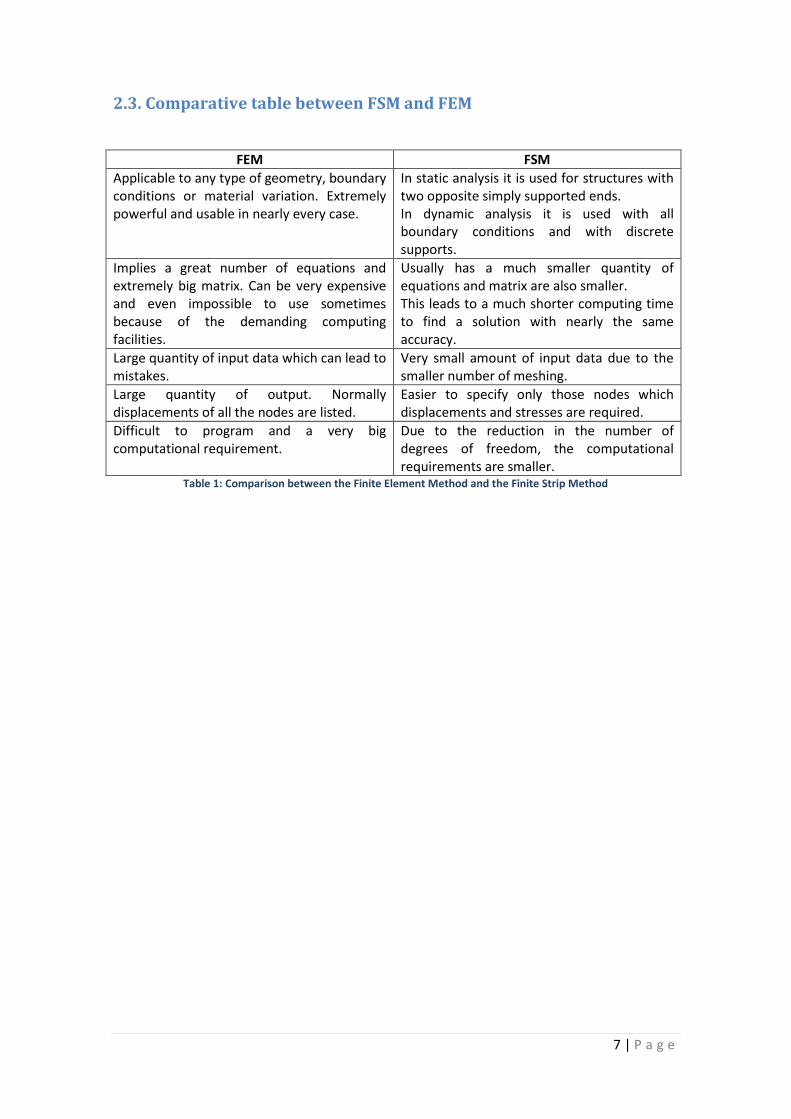
2.3. Comparative table between FSM and FEM
FEM FSM
Applicable to any type of geometry, boundary conditions or material variation. Extremely powerful and usable in nearly every case.
In static analysis it is used for structures with two opposite simply supported ends. In dynamic analysis it is used with all boundary conditions and with discrete supports.
Implies a great number of equations and extremely big matrix. Can be very expensive and even impossible to use sometimes because of the demanding computing facilities.
Usually has a much smaller quantity of equations and matrix are also smaller. This leads to a much shorter computing time to find a solution with nearly the same accuracy.
Large quantity of input data which can lead to mistakes.
Very small amount of input data due to the smaller number of meshing.
Large quantity of output. Normally displacements of all the nodes are listed.
Easier to specify only those nodes which displacements and stresses are required.
Difficult to program and a very big computational requirement.
Due to the reduction in the number of degrees of freedom, the computational requirements are smaller.
Table 1: Comparison between the Finite Element Method and the Finite Strip Method
8 | P a g e
3. Finite Element Method (FEM)
As previously stated, finite element method is a part of the approximate methods, and it
remains the most versatile tool for solving plate exercises.
3.1. History
3.1.2. Creation of the Method
The Finite Element Method was firstly developed in 1943 by Richard Courant, who used the
Ritz method of numerical analysis and minimization of calculus variables to obtain
approximate solutions of a vibration system. A little bit later, in 1956, a document published by
several scientists established a more wide definition of numerical analysis [1]*.
Although there were different approaches depending on the pioneer who developed the
method, all finite element method developments shared one characteristic: mesh
discretization of bigger elements into a set of discrete subdomains, usually called elements.
After the definition of discretization, an equation system was created to apply the equilibrium
equations to every node of every element of the structure. The equations system can be
written in the next way:
𝑓 = 𝐾 · 𝑢
Were the unknowns are the displacement of the nodes (u) and they can be found with the
forces in the nodes (f) and the stiffness matrix (K).
3.1.3. Practical use of the method through the centuries
With the arrival of the first computers in the 1950s decade, the structures calculus was found
in a point where most of the techniques used consisted in iterative methods (like Cross and
Kani) which were realized manually and therefore resulted quite tedious. The calculus of a
building with several floors could take weeks, which in the end supposed a big cost of time.
The arrival of computers allowed for the resurgence of methods for displacement knows of
previous centuries (Navier, Lagrange, Cauchy) but were too difficult to apply given that the use
of them lead to the resolution of enormous equations systems very difficult to approach from
the manual point of view.
Between 1960 and 1970 the application of finite elements kept growing, and the
requirements for calculus time and memory of the computers also grew. At this point the
creation of less demanding and more efficient algorithms became important. In order to solve
the equations systems the already know algorithms (Gauss, Cholesky, Crout, etc…) are
adapted. It is at this point that the matricial method starts to extend. The development of this
method becomes especially known in the structures where discretization into bars is extremely
easy [1]*.
*[1]: Reference to bibliography

9 | P a g e
However, even though the modeling using bars starts to get developed, there is a great
difficulty to solve continuous structures (surfaces and volumes) with complex geometries. It is
particularly in the aerospace camp where new FEM techniques are developed.
In the 1970 there is a great deal of development and the method starts to apply to other
problems such as the nonlinear. During this decade, FEM was limited to expensive computers
and therefore to rich industries such as defense, nuclear, automation or aeronautic.
It is after 1980 that the method finally reaches particulars computers, and the use of
commercial programs that use this method is extended.
Up until today, the FEM system has acquired a lot of importance due to the great increase in
computer capabilities and the reduced economic cost of these. Today, supercomputers are
capable of giving exact results for nearly all kind of parameters.
3.3. FEM example
The Finite Element Method (FEM) is a numerical technique used to find approximate solutions
to boundary value problems for partial differential equations. The method uses variational
methods to minimize an error function and create solutions. To understand the concept, the
idea is analogous to saying that many tiny lines can approximate a large circle, although we will
never get the exact circle. It is based on the discretization (division in smaller elements), which
uses many simple element equations over many small subdomains, named finite elements, to
approximate a solution over a very complex equation in a much larger domain.
3.3.1. Situation
There is no best way to explain a method than using an example. In the finite element method
we take a structure and divide it into smaller elements, using several nodes for it. In our
example a simple beam will be taken, with a force applied in the end.
Figure 2: Initial situation
10 | P a g e
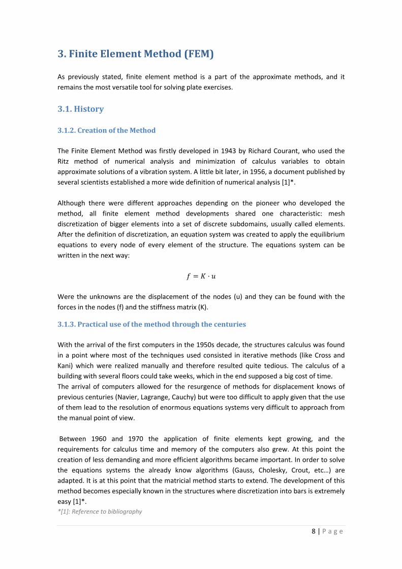
Now, taking the figure into account, we must discretize in order to have the figure divided into
different elements. In this example I will discretize it to have two triangular elements.
Figure 3: Discretization
So we can see that the figure has been discretized into two elements and four nodes. From
now on we will work in the triangular element.
3.3.2 Element solving
3.3.2.1. Displacement functions
We have taken a simple triangular element. In this exercise, we will be working in two
dimensions, but the finite element method can be used in three dimensions all the same.
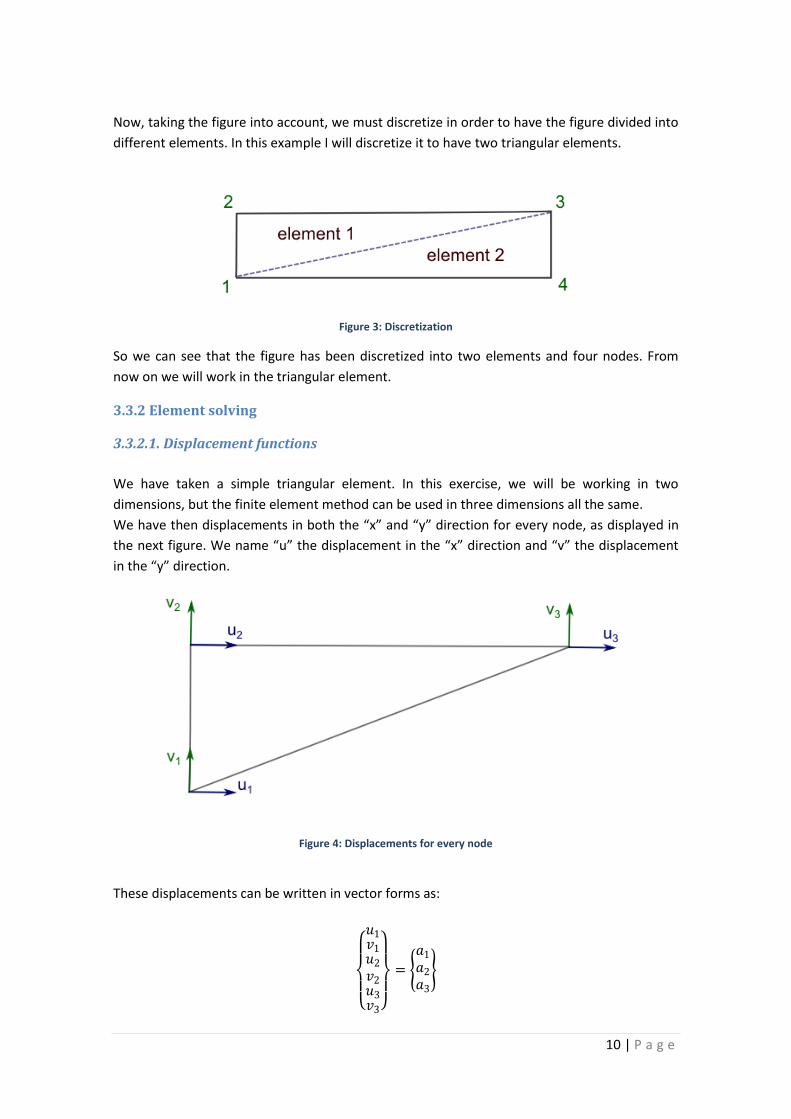
We have then displacements in both the “x” and “y” direction for every node, as displayed in
the next figure. We name “u” the displacement in the “x” direction and “v” the displacement
in the “y” direction.
Figure 4: Displacements for every node
These displacements can be written in vector forms as:
𝑢1𝑣1𝑢2
𝑣2𝑢3𝑣3
=
𝑎1
𝑎2
𝑎3
11 | P a g e
Where each “a” will correspond to the horizontal and vertical displacement of each node. It is
a two vector variable with “u” and “v” inside it.
To know the displacement in any point of the triangle, we create an interpolation function to
interpolate the results in each node in order to find the displacement in a given “x, y”
coordinate.
𝑢 𝑥,𝑦 = 𝑁1 𝑥,𝑦 · 𝑢1 + 𝑁2 𝑥,𝑦 · 𝑢2 + 𝑁3 𝑥,𝑦 · 𝑢3 = 𝑁𝑖 𝑥,𝑦 · 𝑢𝑖
3
𝑖=0
𝑣 𝑥,𝑦 = 𝑁1 𝑥,𝑦 · 𝑣1 + 𝑁2 𝑥,𝑦 · 𝑣2 + 𝑁3 𝑥,𝑦 · 𝑣3 = 𝑁𝑖 𝑥,𝑦 · 𝑣𝑖
3
𝑖=0
Given this equations, we now have to find the interpolation functions N. First we will write the
interpolation function as a function depending of both “x” and “y”:
𝑁1 𝑥,𝑦 = 𝛼1 · 𝑥 + 𝛽1 · 𝑦 + 𝛾1
𝑁2 𝑥,𝑦 = 𝛼2 · 𝑥 + 𝛽2 · 𝑦 + 𝛾2
𝑁3 𝑥,𝑦 = 𝛼3 · 𝑥 + 𝛽3 · 𝑦 + 𝛾3
Once we have this functions, in order to find the coefficients 𝛼,𝛽, 𝛾 we use the boundary
conditions. The next conditions have to be met:
𝑢 𝑥1 ,𝑦1 = 𝑢1 → 𝑁1 𝑥1 ,𝑦1 = 1 ; 𝑁2 𝑥1 ,𝑦1 = 0 ; 𝑁3 𝑥1 ,𝑦1 = 0
𝑢 𝑥2 ,𝑦2 = 𝑢2 → 𝑁1 𝑥2 ,𝑦2 = 0 ; 𝑁2 𝑥2 ,𝑦2 = 1 ; 𝑁3 𝑥2 ,𝑦2 = 0
𝑢 𝑥3 ,𝑦3 = 𝑢3 → 𝑁1 𝑥3 ,𝑦3 = 0 ; 𝑁2 𝑥3 ,𝑦3 = 0 ; 𝑁3 𝑥3 ,𝑦3 = 1
Note that the “x” and “y” are coordinates while “u” and “v” are displacements of those
coordinates. We then have 3 equations with 3 unknowns for every interpolation function N.
Solving this equations we find that:
𝑁1 𝑥,𝑦 =1
2 · ∆· 𝑦2 − 𝑦3 · 𝑥 + 𝑥3 − 𝑥2 · 𝑦 + (𝑥2 · 𝑦3 − 𝑥3 · 𝑦2)
𝑁2 𝑥,𝑦 =1
2 · ∆· 𝑦3 − 𝑦1 · 𝑥 + 𝑥1 − 𝑥3 · 𝑦 + (𝑥1 · 𝑦3 − 𝑥3 · 𝑦1)
𝑁3 𝑥,𝑦 =1
2 · ∆· 𝑦2 − 𝑦1 · 𝑥 + 𝑥2 − 𝑥1 · 𝑦 + (𝑥1 · 𝑦2 − 𝑥2 · 𝑦1)
Where 2·Δ is two times the area of the triangle defined as:
12 | P a g e
2 · ∆= 𝑑𝑒𝑡
1 𝑥1 𝑦1
1 𝑥2 𝑦2
1 𝑥3 𝑦3
= 2 · 𝐴𝑟𝑒𝑎 𝑜𝑓 𝑡𝑒 𝑡𝑟𝑖𝑎𝑛𝑔𝑙𝑒
Finally, having all these parameters, we can define our displacement vector as:
𝑢 𝑣 = 𝑁 · 𝑎
Where “N” is our interpolation matrix and “a” the deformation of known nodes. Expanding this
last equation we would find:
𝑢 𝑣 =
𝑁1 0 𝑁2 0 𝑁3 0
0 𝑁1 0 𝑁2 0 𝑁3 ·
𝑢1
𝑣1𝑢2𝑣2
𝑢3
𝑣3
= 𝑁 · 𝑎
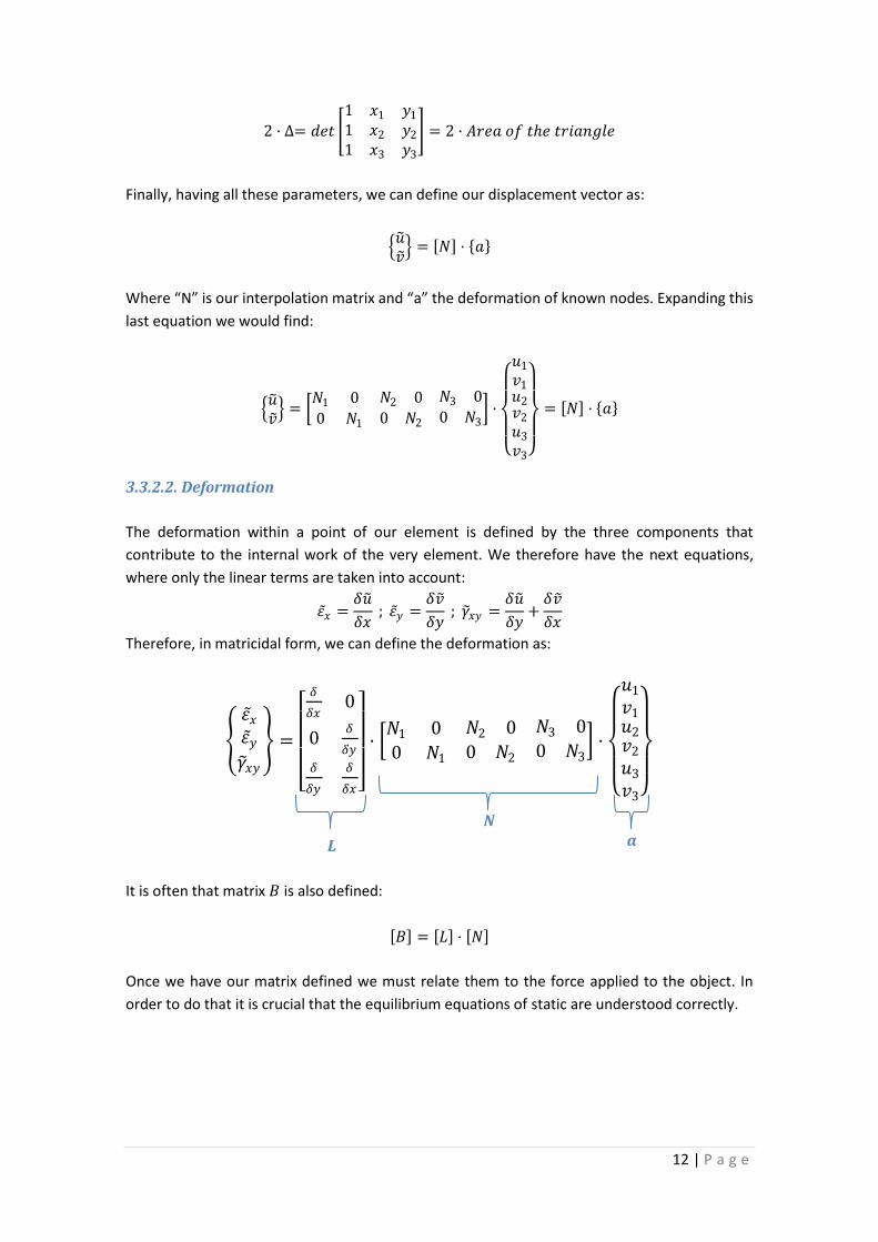
3.3.2.2. Deformation
The deformation within a point of our element is defined by the three components that
contribute to the internal work of the very element. We therefore have the next equations,
where only the linear terms are taken into account:
휀 𝑥 =𝛿𝑢
𝛿𝑥 ; 휀 𝑦 =
𝛿𝑣
𝛿𝑦 ; 𝛾 𝑥𝑦 =
𝛿𝑢
𝛿𝑦+𝛿𝑣
𝛿𝑥
Therefore, in matricidal form, we can define the deformation as:
휀 𝑥휀 𝑦𝛾 𝑥𝑦
=
𝛿
𝛿𝑥0
0𝛿
𝛿𝑦
𝛿
𝛿𝑦
𝛿
𝛿𝑥
· 𝑁1 0 𝑁2 0 𝑁3 0
0 𝑁1 0 𝑁2 0 𝑁3 ·
𝑢1
𝑣1𝑢2𝑣2
𝑢3
𝑣3
It is often that matrix 𝐵 is also defined:
𝐵 = 𝐿 · 𝑁
Once we have our matrix defined we must relate them to the force applied to the object. In
order to do that it is crucial that the equilibrium equations of static are understood correctly.
𝑳
𝑵 𝒂
13 | P a g e
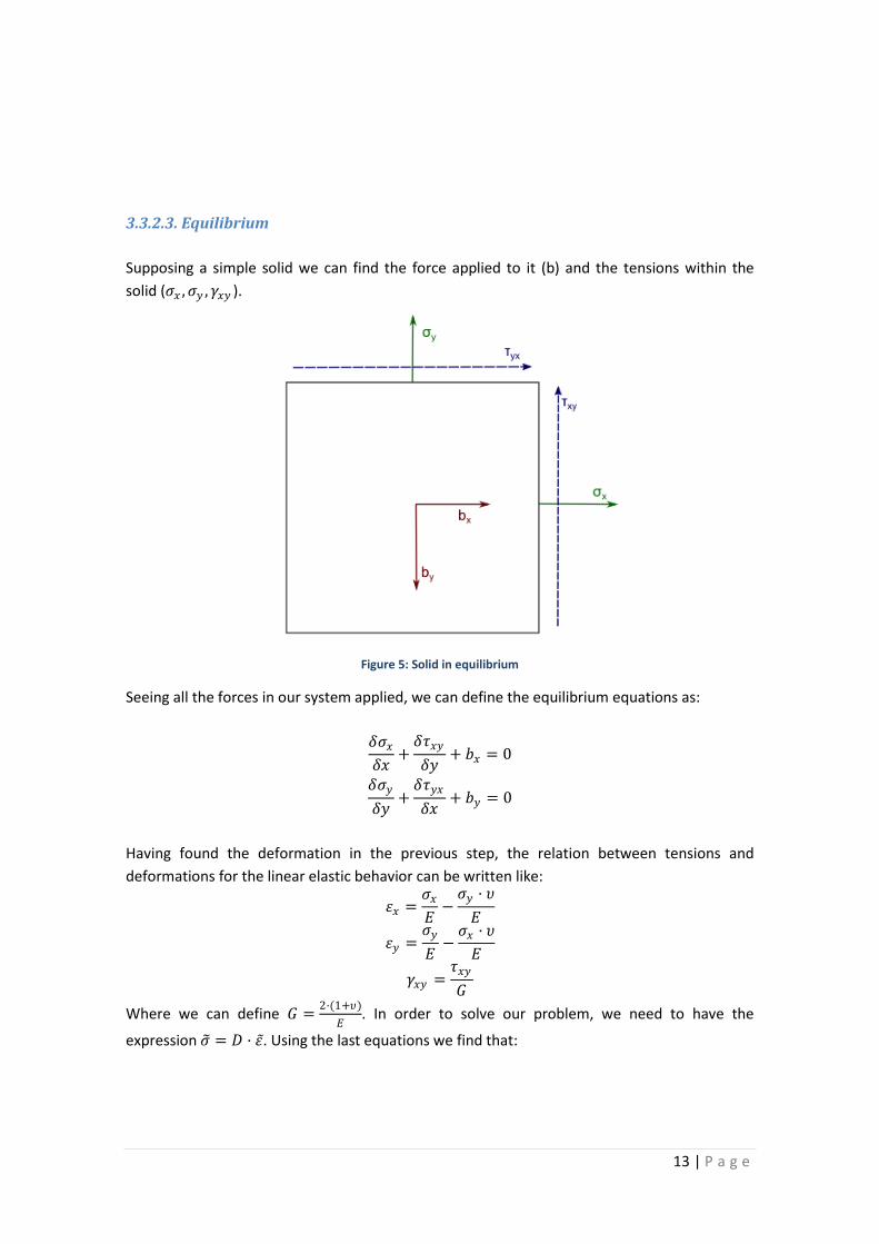
3.3.2.3. Equilibrium
Supposing a simple solid we can find the force applied to it (b) and the tensions within the
solid (𝜎𝑥 ,𝜎𝑦 ,𝛾𝑥𝑦 ).
Figure 5: Solid in equilibrium
Seeing all the forces in our system applied, we can define the equilibrium equations as:
𝛿𝜎𝑥𝛿𝑥
+𝛿𝜏𝑥𝑦
𝛿𝑦+ 𝑏𝑥 = 0
𝛿𝜎𝑦
𝛿𝑦+𝛿𝜏𝑦𝑥
𝛿𝑥+ 𝑏𝑦 = 0
Having found the deformation in the previous step, the relation between tensions and
deformations for the linear elastic behavior can be written like:
휀𝑥 =𝜎𝑥𝐸−𝜎𝑦 · 𝜐
𝐸
휀𝑦 =𝜎𝑦
𝐸−𝜎𝑥 · 𝜐
𝐸
𝛾𝑥𝑦 =𝜏𝑥𝑦
𝐺
Where we can define 𝐺 =2·(1+𝜐)
𝐸. In order to solve our problem, we need to have the
expression 𝜎 = 𝐷 · 휀 . Using the last equations we find that:

14 | P a g e
𝜎 =
𝜎𝑥 𝜎𝑦
𝜏𝑥𝑦 =
𝐸
1 − 𝜐2·
1 𝜐 0𝜐 1 0
0 01 − 𝜐
𝐸
·
휀 𝑥휀 𝑦𝛾 𝑥𝑦
Once we have this it is time to define a new concept, the “virtual work”. This concept refer to
the fact that for every force applied, the object gets an external force which is countered by an
internal force created by the deformations in the object.
We can define the external and the internal energy as:
𝑖𝑛𝑡𝑒𝑟𝑛𝑎𝑙 𝑒𝑛𝑒𝑟𝑔𝑦 = 𝜎 𝑇
𝑉
· 휀 · 𝑑𝑉 = 휀 𝑇
𝑉
· 𝜎 · 𝑑𝑉
𝑒𝑥𝑡𝑒𝑟𝑛𝑎𝑙 𝑒𝑛𝑒𝑟𝑔𝑦 = 𝑁 · 𝑎 𝑇
𝑉
· 𝑏 · 𝑑𝑉
Thanks to the theory of the virtual works we know that these energies have to counter
themselves, so:
휀 𝑇
𝑉
· 𝜎 · 𝑑𝑉 − 𝑁 · 𝑎 𝑇
𝑉
· 𝑏 · 𝑑𝑉 = 0
We can now define the deformation and tension as:
휀 = 𝐵 · 𝑎
𝜎 = 𝐷 · 𝐵 · 𝑎
We then have:
𝐵 𝑇 · 𝑎 𝑇
𝑉
· 𝐷 · 𝐵 · 𝑎 · 𝑑𝑉 − 𝑎 𝑇 · 𝑁 𝑇
𝑉
· 𝑏 · 𝑑𝑉 = 0
Given that the vector 𝑎 does not depend on the volume and that none of the variables above
depend on the thickness (they only depend on the area), we can write the past equation as:
𝑡 𝐵 𝑇 ·𝐴
𝐷 · 𝐵 · 𝑑𝐴 · 𝑎 − 𝑡 𝑁 𝑇
𝐴
· 𝑏 · 𝑑𝐴 = 0
Stiffness matrix (K) Force vector (B)

15 | P a g e
Finally we usually write the past equation as:
𝐾 · 𝑎 − 𝐵 = 𝐾 · 𝑎 − 𝐵 = 0
This so-called “standard discrete system” is solved for the whole structure, taking into account
the boundary conditions.
16 | P a g e
4. Finite Strip Method (FSM)
4.1. History
The finite strip method was created for structural analysis in the late 1960s. It was applied to
several structures such as bridge, tall buildings, plates or shells. The displacements were
described by functions which are given as products of trigonometrical/hyperbolic series and
polynomials. This series should at first satisfy the boundary conditions at the end of the strips.
[4]*
Although the technique is much less powerful and versatile than the Finite Element Method, it
is true that it is much more efficient in computation terms in many situations. It is for this
reason that many times it is more appropriate to use this method.
4.2. Explanation
The finite element method requires a discretization in every dimension of the problem, and
therefore it requires many more unknowns than other methods. If the structures have
geometrical and mechanical properties constant in one of the directions and the transversal
section does not vary in the same direction, then the problem can be simplified. In structures
such as plates or prismatic structures which satisfy the previous statements, the finite element
method can be combined with Fourier series to model the transversal and longitudinal
behavior.
In the finite strip method, the Fourier series are used to express the behavior of the
longitudinal variables while the transversal direction is modeled with the finite element
method. This allows eliminating unknowns associated to the longitudinal direction and solving
the problem by solving the one-dimensional finite element method problem where only
unknowns associated to the transversal direction discretization intervene.
*[4]: Reference to bibliography

17 | P a g e
4.3. The finite strip analysis
4.3.1. Degree of freedom and shape functions
As previously stated, in the finite strip method, the structure is only discretized in the cross-
section. The other dimension is usually represented using a shape trigonometrical function. In
the next figure we can see the axis taken for the exercise. Local coordinates are named with
small letters (x-y-z) and will always be associated with the strip element.
Displacements are represented with the translation U-V-W and the rotation θ for global
displacements and u-v-w and ϕ for local displacements. The subscript p refers to the half-wave
number (number of longitudinal terms).
Figure 6: Strip situation
Figure 7: Strip degrees of freedom definition

18 | P a g e
Figure 8: Strip stress distribution
The shape functions for the transverse direction are assumed to be the same polynomial
function for every boundary condition. On the other hand, in the longitudinal direction,
trigonometrical functions are taken. These functions have to satisfy the pre-set boundary
conditions. The out of plane displacement will use a shape cubic polynomial function for all
boundary conditions. Therefore, the expressions for general displacements are as follows:
𝑢 = 1 −𝑥
𝑏
𝑥
𝑏
𝑚
𝑝=1
· 𝑢1𝑝
𝑢2𝑝 · 𝑌𝑝
𝑣 = 1 −𝑥
𝑏
𝑥
𝑏
𝑚
𝑝=1
· 𝑣1𝑝
𝑣2𝑝 · 𝑌𝑝
′ ·𝑎
𝜇𝑝
𝑤 = 1 −3𝑥2
𝑏2+
2𝑥3
𝑏3𝑥 · 1 −
2𝑥
𝑏+𝑥2
𝑏2 3𝑥2
𝑏2−
2𝑥3
𝑏3𝑥 ·
𝑥2
𝑏2−𝑥
𝑏 ·
𝑤1𝑝
𝜃1𝑝
𝑤2𝑝
𝜃2𝑝
𝑚
𝑝=1
· 𝑌𝑝
Where 𝜇𝑝 = 𝑝 · 𝜋 and 𝑝 is the half-wave number. 𝑌𝑚 is the function for the longitudinal
direction, which varies depending on the boundary conditions.
Boundary condition Shape function
Simply-Simply 𝑌𝑝 = 𝑠𝑖𝑛𝑝 · 𝜋 · 𝑦
𝑎
Clamped-Clamped 𝑌𝑝 = 𝑠𝑖𝑛𝑝 · 𝜋 · 𝑦
𝑎· 𝑠𝑖𝑛
𝜋 · 𝑦
𝑎

19 | P a g e
Simply-Clamped 𝑌𝑝 = 𝑠𝑖𝑛(𝑝 + 1) · 𝜋 · 𝑦
𝑎+
𝑝 + 1
𝑝 𝑠𝑖𝑛
𝑝 · 𝜋 · 𝑦
𝑎
Clamped-Free
𝑌𝑝 = 1 − 𝑐𝑜𝑠 𝑝 −
1
2 · 𝜋 · 𝑦
𝑎
Clamped-Guided 𝑌𝑝 = 𝑠𝑖𝑛 𝑝 −
1
2 · 𝜋 · 𝑦
𝑎· 𝑠𝑖𝑛
𝑝 · 𝜋 · 𝑦
2 · 𝑎
We can put the displacement equations in form of a general vector such that:
𝑢𝑣 = 𝑁𝑢𝑣 ·
𝑢1𝑝
𝑣1𝑝
𝑢2𝑝
𝑣2𝑝
𝑚
𝑝=1
= 𝑁𝑢𝑣 · 𝑑𝑢𝑣𝑝
𝑚
𝑝=1
𝑤 = 𝑁𝑤 ·
𝑤1𝑝
𝜃1𝑝
𝑤2𝑝
𝜃2𝑝
𝑚
𝑝=1
= 𝑁𝑤 · 𝑑𝑤𝑝
𝑚
𝑝=1
𝑚refers to the quantity of half-wave number employed in the analysis. It refers to the shape of
the sinus function we will see in the buckling shape after deformation.
For example, for m=1 and simply-simply boundary conditions in the loaded edges we will have
a full half-sinus in the buckling:
Figure 9: Cufsm4 program “C” section for simply-simply BC and m=1
We can see that the deformation in the 3D shape is a sinus form.
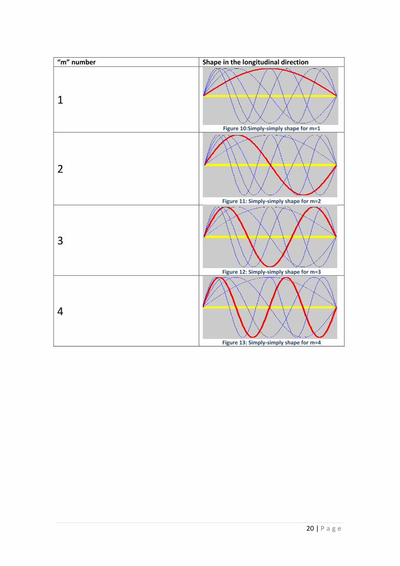
The deformation buckling form depends on the value of the m. We can see the first four “m”
to understand the idea in the next table:
20 | P a g e
“m” number Shape in the longitudinal direction
1
Figure 10:Simply-simply shape for m=1
2
Figure 11: Simply-simply shape for m=2
3
Figure 12: Simply-simply shape for m=3
4
Figure 13: Simply-simply shape for m=4

21 | P a g e
For m=1 we can see the next boundary conditions figures:
4.3.2. Elastic stiffness matrix
In the strip we can distinguish two portions, bending and membrane. Every strip behaves as
the superposition of two independent stresses, the membrane and the bending which is due
to the normal forces to the plane of the plate.
Figure 15: Shape for clamped-clamped boundary conditions
Figure 14: Shape for simply-simply boundary conditions
Figure 17: Shape for simply-clamped boundary conditions
Figure 16: Shape for clamped-free boundary conditions
Figure 18: Shape for clamped-guided boundary conditions

22 | P a g e
The membrane strains are at the mid-line of the strip and will be governed by plane stress
assumptions. On the other hand, bending strains follows Kirchhoff thin plate theory. We can
define the deformation as the sum of both bending and membrane deformations.
휀 = 휀𝑀 + 휀𝐵
4.3.2.1. Membrane matrix
The membrane stress is defined as the component of normal stress that is uniformly
distributed and equal to the average value of the stress across the thickness of the section
under consideration.
In the membrane matrix the plates are submitted to normal and tangential forces in the plane
of the plate, for which we consider a uniform distribution due to the fact that the thickness of
the plate is considered very small compared to the dimensions of the plate. It is also
considered that there is a linear behavior load vs. displacement.
The general expression of the deformation with the linear terms due to membrane stress is:
휀𝑀 =
휀𝑥휀𝑦𝛾𝑥𝑦
𝑀
=
𝜕𝑢
𝜕𝑥𝜕𝑣
𝜕𝑦𝜕𝑢
𝜕𝑦+𝜕𝑣
𝜕𝑥
𝑀
= 𝑁𝑢𝑣′ ·
𝑢1𝑝
𝑣1𝑝
𝑢2𝑝
𝑣2𝑝
𝑚
𝑝=1
= 𝐵𝑀𝑝 · 𝑑𝑢𝑣
𝑝
𝑚
𝑝=1
It is obvious that the displacement due to membrane stress will depend on u and v, which are
the displacements in the plane of the plate, where membrane stress occurs.
Given that the membrane behavior (𝑢, 𝑣) is uncoupled from the bending behavior (𝑤), we can
define the internal strain energy during buckling for membrane stress as:
𝑈𝑀 =1
2· 휀𝑀
𝑇 · 𝜎𝑀 𝑉
· 𝑑𝑉
For the finite strip method we use a constant thickness, which can therefore stay out of the
integration. Also, we can relate 𝜎 to 휀 using the 𝐷 matrix:
𝜎𝑀 = 𝐷𝑀 · 휀𝑀
Where the 𝐷 matrix is:
𝐷𝑀 =1
1 − 𝜈𝑦𝑥 𝜈𝑥𝑦
𝐸𝑥 𝜈𝑥𝑦 · 𝐸𝑥 0
𝜈𝑦𝑥 · 𝐸1 𝐸𝑦 0
0 0 1 − 𝜈𝑥𝑦 𝜈𝑦𝑥 · 𝐺
23 | P a g e
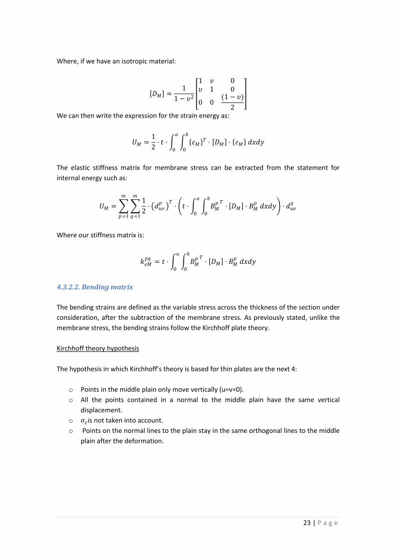
Where, if we have an isotropic material:
𝐷𝑀 =1
1 − 𝜐2
1 𝜐 0𝜐 1 0
0 0(1 − 𝜐)
2
We can then write the expression for the strain energy as:
𝑈𝑀 =1
2· 𝑡 · 휀𝑀
𝑇 · 𝐷𝑀 · 휀𝑀 𝑑𝑥𝑑𝑦𝑏
0
𝑎
0
The elastic stiffness matrix for membrane stress can be extracted from the statement for
internal energy such as:
𝑈𝑀 = 1
2· 𝑑𝑢𝑣
𝑝 𝑇
· 𝑡 · 𝐵𝑀𝑝 𝑇
· 𝐷𝑀 · 𝐵𝑀𝑝
𝑑𝑥𝑑𝑦𝑏
0
𝑎
0
𝑚
𝑞=1
𝑚
𝑝=1
· 𝑑𝑢𝑣𝑞
Where our stiffness matrix is:
𝑘𝑒𝑀𝑝𝑞
= 𝑡 · 𝐵𝑀𝑝 𝑇
· 𝐷𝑀 · 𝐵𝑀𝑝
𝑑𝑥𝑑𝑦𝑏
0
𝑎
0
4.3.2.2. Bending matrix
The bending strains are defined as the variable stress across the thickness of the section under
consideration, after the subtraction of the membrane stress. As previously stated, unlike the
membrane stress, the bending strains follow the Kirchhoff plate theory.
Kirchhoff theory hypothesis
The hypothesis in which Kirchhoff’s theory is based for thin plates are the next 4:
o Points in the middle plain only move vertically (u=v=0).
o All the points contained in a normal to the middle plain have the same vertical
displacement.
o 𝜎𝑧 is not taken into account.
o Points on the normal lines to the plain stay in the same orthogonal lines to the middle
plain after the deformation.

24 | P a g e
Thanks to the previous hypothesis, we can write our displacements as:
𝑢 𝑥,𝑦, 𝑧 = −𝑧 · 𝜃𝑥(𝑥,𝑦)
𝑣 𝑥,𝑦, 𝑧 = −𝑧 · 𝜃𝑦(𝑥,𝑦)
𝑤 𝑥,𝑦, 𝑧 = 𝑤(𝑥,𝑦)
Where
o 𝜔is the vertical displacement.
o 𝜃𝑥 𝑎𝑛𝑑 𝜃𝑦are the angles that define the turn of the normal line to the middle plain.
Figure 19: Kirchhoff deformation hypothesis image
Taking this image into account we can see that:
In the xz plain: 𝜃𝑥 =𝜕𝑤
𝜕𝑥
In the yz plain: 𝜃𝑦 =𝜕𝑤
𝜕𝑦
Using these equations and the ones written before we can conclude that:
𝑢 𝑥,𝑦, 𝑧 = −𝑧 ·𝜕𝑤(𝑥,𝑦)
𝜕𝑥
1st and 4th hypothesis
2nd hypothesis

25 | P a g e
𝑣 𝑥,𝑦, 𝑧 = −𝑧 ·𝜕𝑤(𝑥,𝑦)
𝜕𝑦
𝑤 𝑥,𝑦, 𝑧 = 𝑤(𝑥,𝑦)
Taking the last expression, we can define the deformation as:
휀𝐵 =
휀𝑥휀𝑦𝛾𝑥𝑦
=
−𝑧 ·
𝜕2𝑤
𝜕𝑥2
−𝑧 ·𝜕2𝑤
𝜕𝑦2
2𝑧 ·𝜕2𝑤
𝜕𝑥𝜕𝑦
= 𝑧 · 𝑁𝑤′ ·
𝑤1𝑝
𝜃1𝑝
𝑤2𝑝
𝜃2𝑝
𝑚
𝑝=1
= 𝑧 · 𝐵𝐵𝑝 · 𝑑𝑤
𝑝
𝑚
𝑝=1
As in the case of the membrane stress, we can write the bending term of the internal strain
energy during buckling as:
𝑈𝐵 =1
2· 휀𝐵
𝑇 · 𝜎𝐵 𝑉
𝑑𝑉
Where we can substitute:
𝜎𝐵 = 𝐷𝐵 · 휀𝐵
𝐷𝐵 =𝑡3
12·
1
1 − 𝜈𝑦𝑥 𝜈𝑥𝑦
𝐸𝑥 𝜈𝑥𝑦 · 𝐸𝑥 0
𝜈𝑦𝑥 · 𝐸1 𝐸𝑦 0
0 0 1 − 𝜈𝑥𝑦 𝜈𝑦𝑥 · 𝐺
In the case of an isotropic material:
𝐷𝐵 =𝑡3
12·
1
1 − 𝜐2
1 𝜐 0𝜐 1 0
0 0(1 − 𝜐)
2
We can then write the expression for the strain energy as:
𝑈𝐵 =1
2· 휀𝐵
𝑇 · 𝐷𝐵 · 휀𝐵 𝑑𝑥𝑑𝑦𝑏
0
𝑎
0
The elastic stiffness matrix for membrane stress can be extracted from the statement for
internal energy such as:
𝑈𝐵 = 1
2· 𝑑𝑤
𝑝 𝑇
· 𝐵𝐵𝑝𝑇
· 𝐷𝐵 · 𝐵𝐵𝑝
𝑑𝑥𝑑𝑦𝑏
0
𝑎
0
𝑚
𝑞=1
𝑚
𝑝=1
· 𝑑𝑤𝑞

26 | P a g e
Where our stiffness matrix is:
𝑘𝑒𝐵𝑝𝑞
= 𝐵𝐵𝑝𝑇
· 𝐷𝐵 · 𝐵𝐵𝑝
𝑑𝑥𝑑𝑦𝑏
0
𝑎
0
4.3.2.3. Local stiffness matrix
The local stiffness matrix will be a combination of both the membrane and the bending strains.
We can define it as:
𝐾𝑒𝑝𝑞
= 𝑘𝑒𝑀𝑝𝑞
0
0 𝑘𝑒𝐵𝑝𝑞
During the development of the global stiffness matrix the next general expressions for both
membrane and bending matrixes have been found. These expressions correspond to the value
after the integration:
𝑘𝑒𝑀𝑝𝑞
= 𝑡 ·
𝐸1𝐼1𝑏
+𝐺𝑏𝐼5
3 −
𝐸2𝜐𝑥𝐼22𝑐1
−𝐺𝐼52𝑐1
−𝐸1𝐼1𝑏
+𝐺𝑏𝐼5
6 −
𝐸2𝜐𝑥𝐼22𝑐1
+𝐺𝐼52𝑐1
−𝐸2𝜐𝑥𝐼2
2𝑐1−𝐺𝐼52𝑐1
𝐸2𝑏𝐼43𝑐1𝑐2
+𝐺𝐼5𝑏𝑐1𝑐2
𝐸2𝜐𝑥𝐼2
2𝑐1−𝐺𝐼52𝑐1
𝐸2𝑏𝐼46𝑐1𝑐2
−𝐺𝐼5𝑏𝑐1𝑐2
−𝐸1𝐼1𝑏
+𝐺𝑏𝐼5
6
𝐸2𝜐𝑥𝐼22𝑐1
−𝐺𝐼52𝑐1
𝐸1𝐼1𝑏
+𝐺𝑏𝐼5
3
𝐸2𝜐𝑥𝐼32𝑐1
+𝐺𝐼52𝑐1
−𝐸2𝜐𝑥𝐼2
2𝑐1+𝐺𝐼52𝑐1
𝐸2𝑏𝐼46𝑐1𝑐2
−𝐺𝐼5𝑏𝑐1𝑐2
𝐸2𝜐𝑥𝐼3
2𝑐1+𝐺𝐼52𝑐1
𝐸2𝑏𝐼43𝑐1𝑐2
+𝐺𝐼5𝑏𝑐1𝑐2
𝑘𝑒𝐵𝑝𝑞
=1
420𝑏3
5040𝐷𝑥𝐼1 − 504𝑏2𝐷1𝐼2−504𝑏2𝐷1𝐼3 + 156𝑏4𝐷𝑦𝐼4
+2016𝑏2𝐷𝑥𝑦 𝐼5
2520𝑏𝐷𝑥 𝐼1 − 462𝑏3𝐷1𝐼2−42𝑏3𝐷1𝐼3 + 22𝑏5𝐷𝑦𝐼4
+168𝑏3𝐷𝑥𝑦 𝐼5
−5040𝐷𝑥𝐼1 + 504𝑏2𝐷1𝐼2+504𝑏2𝐷1𝐼3 + 54𝑏4𝐷𝑦𝐼4
−2016𝑏2𝐷𝑥𝑦 𝐼5
2520𝑏𝐷𝑥𝐼1 − 42𝑏3𝐷1𝐼2−42𝑏3𝐷1𝐼3 − 13𝑏5𝐷𝑦𝐼4
+168𝑏3𝐷𝑥𝑦 𝐼5
2520𝑏𝐷𝑥𝐼1 − 462𝑏3𝐷1𝐼2−42𝑏3𝐷1𝐼3 + 22𝑏5𝐷𝑦𝐼4
+168𝑏3𝐷𝑥𝑦 𝐼5
1680𝑏2𝐷𝑥𝐼1 − 56𝑏4𝐷1𝐼2−56𝑏4𝐷1𝐼3 + 4𝑏6𝐷𝑦𝐼4
+224𝑏4𝐷𝑥𝑦 𝐼5
−2520𝑏𝐷𝑥𝐼1 + 42𝑏3𝐷1𝐼2+42𝑏3𝐷1𝐼3 + 13𝑏5𝐷𝑦𝐼4
−168𝑏3𝐷𝑥𝑦 𝐼5
840𝑏2𝐷𝑥𝐼1 + 14𝑏4𝐷1𝐼2+14𝑏4𝐷1𝐼3 − 3𝑏6𝐷𝑦𝐼4
−56𝑏4𝐷𝑥𝑦 𝐼5
−5040𝐷𝑥𝐼1 + 504𝑏2𝐷1𝐼2+504𝑏2𝐷1𝐼3 + 54𝑏4𝐷𝑦𝐼4
−2016𝑏2𝐷𝑥𝑦 𝐼5
−2520𝑏𝐷𝑥 𝐼1 + 42𝑏3𝐷1𝐼2+42𝑏3𝐷1𝐼3 + 13𝑏5𝐷𝑦𝐼4
−168𝑏3𝐷𝑥𝑦 𝐼5
5040𝐷𝑥𝐼1 − 504𝑏2𝐷1𝐼2−504𝑏2𝐷1𝐼3 + 156𝑏4𝐷𝑦𝐼4
+2016𝑏2𝐷𝑥𝑦 𝐼5
−2520𝑏𝐷𝑥𝐼1 + 462𝑏3𝐷1𝐼2+42𝑏3𝐷1𝐼3 − 22𝑏5𝐷𝑦𝐼4
−168𝑏3𝐷𝑥𝑦 𝐼5
2520𝑏𝐷𝑥𝐼1 − 42𝑏3𝐷1𝐼2−42𝑏3𝐷1𝐼3 − 13𝑏5𝐷𝑦𝐼4
+168𝑏3𝐷𝑥𝑦 𝐼5
−5040𝐷𝑥𝐼1 + 504𝑏2𝐷1𝐼2+504𝑏2𝐷1𝐼3 + 54𝑏4𝐷𝑦𝐼4
−2016𝑏2𝐷𝑥𝑦 𝐼5
−5040𝐷𝑥𝐼1 + 504𝑏2𝐷1𝐼2+504𝑏2𝐷1𝐼3 + 54𝑏4𝐷𝑦𝐼4
−2016𝑏2𝐷𝑥𝑦 𝐼5
1680𝑏2𝐷𝑥𝐼1 − 56𝑏4𝐷1𝐼2−56𝑏4𝐷1𝐼3 + 4𝑏6𝐷𝑦𝐼4
+224𝑏4𝐷𝑥𝑦 𝐼5
Where
𝑐1 =𝑝𝜋
𝑎
𝑐2 =𝑞𝜋
𝑎
I depends on the boundary conditions and is:
𝐼1 = 𝑌𝑝 · 𝑌𝑞 · 𝑑𝑦𝑎
0

27 | P a g e
𝐼2 = 𝑌𝑝′′ · 𝑌𝑞 · 𝑑𝑦
𝑎
0
𝐼3 = 𝑌𝑝 · 𝑌𝑞′′ · 𝑑𝑦
𝑎
0
𝐼4 = 𝑌𝑝′′ · 𝑌𝑞
′′ · 𝑑𝑦𝑎
0
𝐼5 = 𝑌𝑝′ · 𝑌𝑞
′ · 𝑑𝑦𝑎
0
And the coefficient E and D correspond to:
𝐸1 =𝐸𝑥
1 − 𝑣𝑥𝑣𝑦
𝐸2 =𝐸𝑦
1 − 𝑣𝑥𝑣𝑦
𝐷𝑥 =𝐸𝑥𝑡
3
12(1 − 𝑣𝑥𝑣𝑦)
𝐷𝑦 =𝐸𝑦𝑡
3
12(1 − 𝑣𝑥𝑣𝑦)
𝐷1 =𝑣𝑥𝐸𝑦𝑡
3
12(1 − 𝑣𝑥𝑣𝑦)=
𝑣𝑦𝐸𝑥𝑡3
12(1 − 𝑣𝑥𝑣𝑦)
𝐷𝑥𝑦 =𝐺𝑡3
12
Finally we can describe the full local matrix depending on the half-wave number as:
𝐾𝑒 = 𝑘𝑒𝑀𝑝𝑞
·
· 𝑘𝑒𝐵𝑝𝑞
𝑚𝑥𝑚
Where 𝑚 is the maximum half-wave number. For example for 𝑚 = 2 we will have a matrix:
𝐾𝑒 = 𝐾𝑒
11 𝐾𝑒12
𝐾𝑒21 𝐾𝑒
22
Therefore, the dimension of our matrix would be equal to:
𝑑𝑖𝑚𝑒𝑛𝑠𝑖𝑜𝑛 = 𝑚 · 𝑛𝑛𝑜𝑑𝑒𝑠 · 𝑑𝑖𝑠𝑝𝑙𝑎𝑐𝑒𝑚𝑒𝑛𝑡𝑠
Where
𝑚 = 𝑚𝑎𝑥𝑖𝑚𝑢𝑚 𝑎𝑙𝑓𝑤𝑎𝑣𝑒 𝑛𝑢𝑚𝑏𝑒𝑟𝑠
𝑛𝑛𝑜𝑑𝑒𝑠 = 𝑡𝑜𝑡𝑎𝑙 𝑛𝑢𝑚𝑏𝑒𝑟 𝑜𝑓 𝑛𝑜𝑑𝑒𝑠
𝑑𝑖𝑠𝑝𝑙𝑎𝑐𝑒𝑚𝑒𝑛𝑡𝑠 = 4 𝑑𝑖𝑠𝑝𝑙𝑎𝑐𝑒𝑚𝑒𝑛𝑡𝑠 𝑓𝑜𝑟 𝑒𝑣𝑒𝑟𝑦 𝑛𝑜𝑑𝑒
28 | P a g e
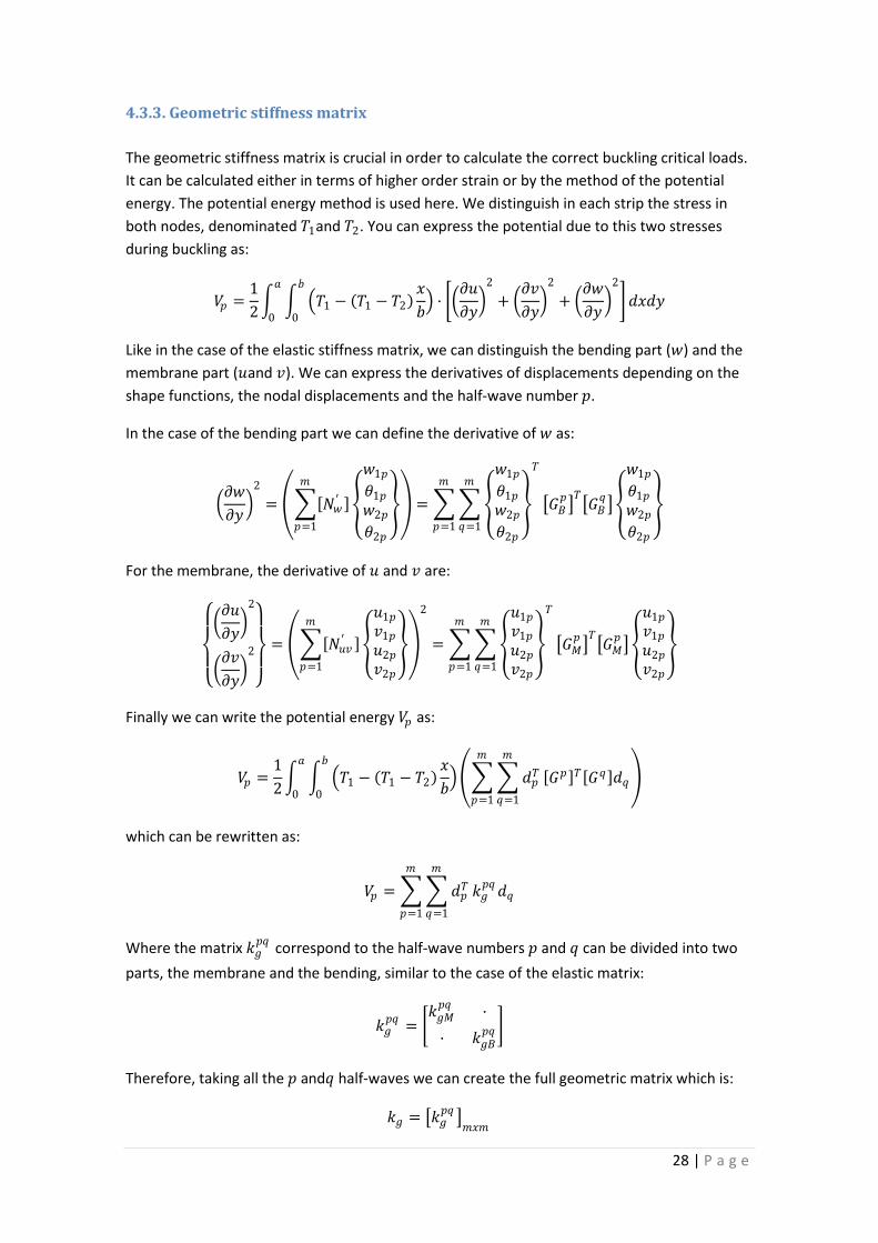
4.3.3. Geometric stiffness matrix
The geometric stiffness matrix is crucial in order to calculate the correct buckling critical loads.
It can be calculated either in terms of higher order strain or by the method of the potential
energy. The potential energy method is used here. We distinguish in each strip the stress in
both nodes, denominated 𝑇1and 𝑇2. You can express the potential due to this two stresses
during buckling as:
𝑉𝑝 =1
2 𝑇1 − 𝑇1 − 𝑇2
𝑥
𝑏 ·
𝜕𝑢
𝜕𝑦
2
+ 𝜕𝑣
𝜕𝑦
2
+ 𝜕𝑤
𝜕𝑦
2
𝑏
0
𝑎
0
𝑑𝑥𝑑𝑦
Like in the case of the elastic stiffness matrix, we can distinguish the bending part (𝑤) and the
membrane part (𝑢and 𝑣). We can express the derivatives of displacements depending on the
shape functions, the nodal displacements and the half-wave number 𝑝.
In the case of the bending part we can define the derivative of 𝑤 as:
𝜕𝑤
𝜕𝑦
2
= 𝑁𝑤′
𝑤1𝑝
𝜃1𝑝
𝑤2𝑝
𝜃2𝑝
𝑚
𝑝=1
=
𝑤1𝑝
𝜃1𝑝
𝑤2𝑝
𝜃2𝑝
𝑇
𝐺𝐵𝑝 𝑇 𝐺𝐵
𝑞
𝑤1𝑝
𝜃1𝑝
𝑤2𝑝
𝜃2𝑝
𝑚
𝑞=1
𝑚
𝑝=1
For the membrane, the derivative of 𝑢 and 𝑣 are:
𝜕𝑢
𝜕𝑦
2
𝜕𝑣
𝜕𝑦
2
= 𝑁𝑢𝑣′
𝑚
𝑝=1
𝑢1𝑝
𝑣1𝑝
𝑢2𝑝
𝑣2𝑝
2
=
𝑢1𝑝
𝑣1𝑝
𝑢2𝑝
𝑣2𝑝
𝑇𝑚
𝑞=1
𝑚
𝑝=1
𝐺𝑀𝑝 𝑇 𝐺𝑀
𝑝
𝑢1𝑝
𝑣1𝑝
𝑢2𝑝
𝑣2𝑝
Finally we can write the potential energy 𝑉𝑝 as:
𝑉𝑝 =1
2 𝑇1 − 𝑇1 − 𝑇2
𝑥
𝑏 𝑑𝑝
𝑇
𝑚
𝑞=1
𝑚
𝑝=1
𝐺𝑝 𝑇 𝐺𝑞 𝑑𝑞 𝑏
0
𝑎
0
which can be rewritten as:
𝑉𝑝 = 𝑑𝑝𝑇
𝑚
𝑞=1
𝑚
𝑝=1
𝑘𝑔𝑝𝑞𝑑𝑞
Where the matrix 𝑘𝑔𝑝𝑞
correspond to the half-wave numbers 𝑝 and 𝑞 can be divided into two
parts, the membrane and the bending, similar to the case of the elastic matrix:
𝑘𝑔𝑝𝑞
= 𝑘𝑔𝑀𝑝𝑞
·
· 𝑘𝑔𝐵𝑝𝑞
Therefore, taking all the 𝑝 and𝑞 half-waves we can create the full geometric matrix which is:
𝑘𝑔 = 𝑘𝑔𝑝𝑞 𝑚𝑥𝑚

29 | P a g e
Where 𝑚 is the maximum number of half-waves used in the analysis.
The values of the bending and membrane matrix after integration corresponding to the half-
waves 𝑝 and 𝑞 can be obtained through the substitution in the next matrices:
𝑘𝑔𝑀𝑝𝑞
=
3𝑇1 + 𝑇2 𝑏𝐼5
120
𝑇1 + 𝑇2 𝑏𝐼512
0
0 3𝑇1 + 𝑇2 𝑏𝑎
2𝐼412𝜇𝑝𝜇𝑞
0 𝑇1 + 𝑇2 𝑏𝑎
2𝐼412𝜇𝑝𝜇𝑞
𝑇1 + 𝑇2 𝑏𝐼512
0 3𝑇1 + 𝑇2 𝑏𝐼5
120
0 𝑇1 + 𝑇2 𝑏𝑎
2𝐼412𝜇𝑝𝜇𝑞
0 3𝑇1 + 𝑇2 𝑏𝑎
2𝐼412𝜇𝑝𝜇𝑞
𝑘𝑔𝐵𝑝𝑞
=
10𝑇1 + 3𝑇2 𝑏𝐼5
35
15𝑇1 + 7𝑇2 𝑏2𝐼5
420
𝑇1 + 𝑇2 𝑏𝐼5140
− 7𝑇1 + 6𝑇2 𝑏
2𝐼5420
15𝑇1 + 7𝑇2 𝑏2𝐼5
420
5𝑇1 + 3𝑇2 𝑏3𝐼5
840
6𝑇1 + 7𝑇2 𝑏2𝐼5
420− 𝑇1 + 𝑇2 𝑏
3𝐼5280
𝑇1 + 𝑇2 𝑏𝐼5140
6𝑇1 + 7𝑇2 𝑏2𝐼5
420
3𝑇1 + 10𝑇2 𝑏𝐼535
− 7𝑇1 + 15𝑇2 𝑏
2𝐼5420
− 7𝑇1 + 6𝑇2 𝑏
2𝐼5420
− 𝑇1 + 𝑇2 𝑏
3𝐼5280
− 7𝑇1 + 15𝑇2 𝑏
2𝐼5420
3𝑇1 + 5𝑇2 𝑏3𝐼5
840
Where
𝜇𝑝 = 𝑝𝜋
𝜇𝑞 = 𝑞𝜋
I depends on the boundary conditions and is:
𝐼1 = 𝑌𝑝 · 𝑌𝑞 · 𝑑𝑦𝑎
0
𝐼2 = 𝑌𝑝′′ · 𝑌𝑞 · 𝑑𝑦
𝑎
0
𝐼3 = 𝑌𝑝 · 𝑌𝑞′′ · 𝑑𝑦
𝑎
0
𝐼4 = 𝑌𝑝′′ · 𝑌𝑞
′′ · 𝑑𝑦𝑎
0
𝐼5 = 𝑌𝑝′ · 𝑌𝑞
′ · 𝑑𝑦𝑎
0
And 𝑇1and 𝑇2 are the stresses in the nodes of the element.
30 | P a g e
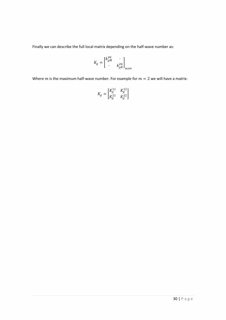
Finally we can describe the full local matrix depending on the half-wave number as:
𝐾𝑔 = 𝑘𝑔𝑀𝑝𝑞
·
· 𝑘𝑔𝐵𝑝𝑞
𝑚𝑥𝑚
Where 𝑚 is the maximum half-wave number. For example for 𝑚 = 2 we will have a matrix:
𝐾𝑔 = 𝐾𝑔
11 𝐾𝑔12
𝐾𝑔21 𝐾𝑔
22

31 | P a g e
4.3.4. Assembly of the elements
We have now found the local elastic stiffness matrix and the local geometric stiffness matrix.
In order to create the full global matrices we must first transform the local matrices to the
global coordinates and then assemble all the matrices together to find the full global matrices.
4.3.4.1. Rotation
In order to rotate the strip we have to create the matrix for rotation which relates movements
between local and global coordinates. In order to understand this matrix we can use the next
image:
Figure 20: Strip rotation guide image
𝑈1
𝑉1
𝑈2
𝑉2
𝑊1
𝜃1
𝑊2
𝜃2
=
cos(𝛼) 0 0 0 −sin(𝛼) 0 0 0
0 1 0 0 0 0 0 00 0 cos(𝛼) 0 0 0 −sin(𝛼) 00 0 0 1 0 0 0 0
sin(𝛼) 0 0 0 cos(𝛼) 0 0 00 0 0 0 0 1 0 00 0 sin(𝛼) 0 0 0 cos(𝛼) 00 0 0 0 0 0 0 1
·
𝑢1
𝑣1
𝑢2
𝑣2
𝑤1
𝜃1
𝑤2
𝜃2
This matrix relates the local coordinates to the global coordinates. This matrix has to be
extended to the 𝑚 number of halfwaves analyzed.
32 | P a g e
4.3.4.2. Assembly
After changing the local matrices to the global coordinates we must assemble them together
to create the full global matrix.
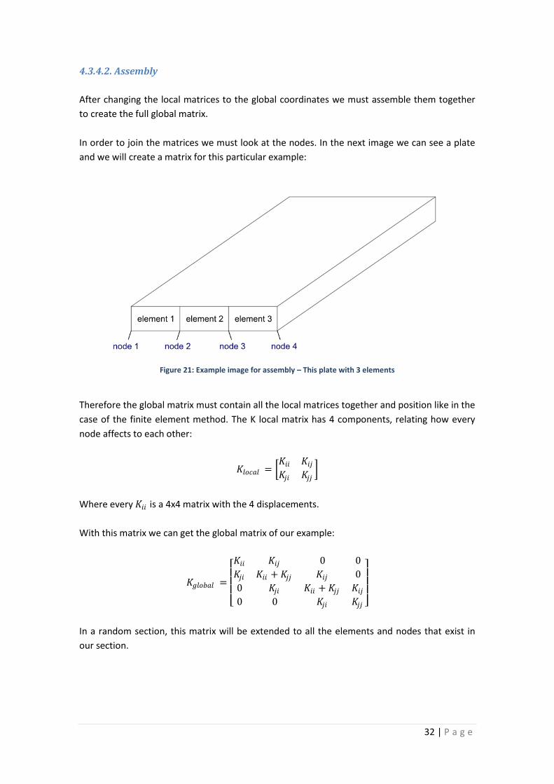
In order to join the matrices we must look at the nodes. In the next image we can see a plate
and we will create a matrix for this particular example:
Figure 21: Example image for assembly – This plate with 3 elements
Therefore the global matrix must contain all the local matrices together and position like in the
case of the finite element method. The K local matrix has 4 components, relating how every
node affects to each other:
𝐾𝑙𝑜𝑐𝑎𝑙 = 𝐾𝑖𝑖 𝐾𝑖𝑗𝐾𝑗𝑖 𝐾𝑗𝑗
Where every 𝐾𝑖𝑖 is a 4x4 matrix with the 4 displacements.
With this matrix we can get the global matrix of our example:
𝐾𝑔𝑙𝑜𝑏𝑎𝑙 =
𝐾𝑖𝑖 𝐾𝑖𝑗 0 0
𝐾𝑗𝑖 𝐾𝑖𝑖 + 𝐾𝑗𝑗 𝐾𝑖𝑗 0
0 𝐾𝑗𝑖 𝐾𝑖𝑖 + 𝐾𝑗𝑗 𝐾𝑖𝑗0 0 𝐾𝑗𝑖 𝐾𝑗𝑗
In a random section, this matrix will be extended to all the elements and nodes that exist in
our section.
33 | P a g e
4.4. Buckling modes
Thin-walled members, when subjected to a large compressive normal stress, usually fail by the
loss of stability, more than due to reaching the material limit parameters. Usually we can
distinguish three basic modes of buckling: local, distortional and global buckling. All three
modes eventually cause excessive deformation and lead to failure. [7]*
It is very important to understand the buckling modes and the critical stress associated to each
mode. Every mode has a different degree of post-buckling capacity, but they all lead to an
eventual collapse response. Therefore, we most calculate the critical stress to avoid the loss of
stability.
Even when the designs do require the calculation of buckling stresses, there are no clear
definitions for each of the modes and it is quite difficult to ultimately distinguish between
them correctly.
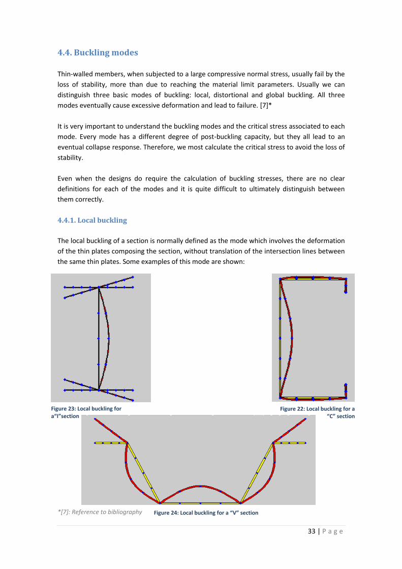
4.4.1. Local buckling
The local buckling of a section is normally defined as the mode which involves the deformation
of the thin plates composing the section, without translation of the intersection lines between
the same thin plates. Some examples of this mode are shown:
*[7]: Reference to bibliography
Figure 23: Local buckling for a“I”section
Figure 22: Local buckling for a “C” section
Figure 24: Local buckling for a “V” section

34 | P a g e
4.4.2. Distortional buckling
Distortional buckling is a mode defined as a cross-sectional distortion that involves the
translation of some of the fold lines (intersection lines between thin plates). It is a rare mode
of buckling, we can see a clear example of it in the C section:
Figure 25: Distortional buckling for a “C” section
4.4.3. Global buckling
Global buckling is a mode where the member deforms with no deformation in its section.
Figure 27: Global buckling for a “V” section
Figure 26: Global buckling for a “C” section

35 | P a g e
4.4.4. Generalized Beam Theory
Thanks to the Generalized Beam Theory (GBT), the modes can be correctly described and with
some programs we can even isolate different buckling modes. In order to distinguish between
the buckling modes, the GBT establishes three criteria:
Criteria 1
o 𝛾𝑥𝑦 = 0, membrane (in-plane) shear strains are zero.
o 휀𝑥 = 0, membrane transverse strains are zero.
o 𝑣 = 𝑓(𝑥), longitudinal displacements are linear in x within an element.
Criteria 2
o 휀𝑦 ≠ 0, longitudinal strains/displacements are non-zero along the length.
Criteria 3
o 𝜅𝑦 = 0, no flexure in the transverse direction.
The buckling modes can then be described as:
Global buckling: Global buckling modes are those that satisfy all the three criteria.
Distortional buckling: Distortional buckling modes are those that satisfy criteria 1 and
2 but do not satisfy criteria 3.
Local buckling: Local buckling modes satisfy criterion 1, but do not satisfy criterion 2.
Criterion 3 is irrelevant in this case.
In the next table we can see a resume of the classification of modes.
Global modes Distortional modes Local modes
𝛾𝑥𝑦 = 0, 휀𝑥 = 0, 𝑣 = 𝑓(𝑥) YES YES YES
휀𝑦 ≠ 0 YES YES NO
𝜅𝑦 = 0 YES NO -
The program “CUFSM 4.05” has been used to obtain the images of the previous buckling
modes.

36 | P a g e
5. Matlab program
In order to solve structures using the finite strip method, in this project we have developed a
program that will solve any section structures utilizing the finite strip method.
We will explain both the functioning of the program as all the sub-programs that have been
implemented. We will then proceed to explain how to use the program and use a few
examples to understand the functioning.
5.1. Main program
The main programs that has been developed returns, for several strip lengths and any section,
the critical buckling value and the buckling mode.It also calculates the particular displacement
caused by the submitted stress.
Our main program is named “FSMsolver” and the function is:
[shape,curve,sigmacritical] = FSMcrit(material_properties,nodes,elements,lengths,boundary_conditions,m_a)
INPUTS OUTPUTS
Material properties: [Ex Eyvxvy G] Nodes [node_numberx_positionz_position stress] Elements [element_numbernodeinodej t] Lengths Boundary conditions m_a
Shape Curve Critical buckling stress Displacement
Inputs
o Material properties: One of the inputs that are demanded is the material properties.
o Ex = 𝐸𝑥 : Young modulus in the “x” direction.
o Ey= 𝐸𝑦 : Young modulus in the “y” direction.
o vx =𝜈𝑥 : Poisson’s ratio in the “x” direction.
o vy = 𝜈𝑦 : Poisson’s ratio in the “y” direction.
o Gxy = The shear modulus for the material. It can be calculated using the Young
modulus and the Poisson’s ratio:
𝐺𝑥𝑦 =𝐸𝑥
2 · (1 + 𝜐𝑥𝑦 )
o Nodes: The nodes of the section we want to analyze
o node_number = The node number that we will then we can then identify to
know the modal displacement in the “shape” output.
o x_position = The “x” coordinate for the node.
o z_position = The “z” coordinate for the node.
o stress = The normal stress we want the node to suffer.

37 | P a g e
o Elements: The elements connecting the nodes must also be defined
o element_number = The element number
o nodei and nodej = The two nodes the element is connecting
o t = The thickness of the element connecting both nodes
o Lengths: The length of the strips we are analyzing.
o Boundary conditions: The boundary conditions at the loaded edges.
o 'S-S': Simply-simply supported boundary condition at loaded edges.
o 'C-C': Clamped-clamped boundary condition at loaded edges.
o 'S-C': Simply-clamped boundary condition at loaded edges.
o 'C-F': Clamped-free supported boundary condition at loaded edges.
o 'C-G': Clamped-guided supported boundary condition at loaded edges.
o m_a: half-wave terms to be analyzed for the length.
Output
o Shape: A matrix containing the modal displacement for all nodes after the finite strip
analysis. The matrix will contain the next values.
· · · · · ·· · · · · ·· · · · · ·· · · · · ·· · · · · ·· · · · · ·· · · · · ·· · · · · ·· · · · · ·· · · · · ·
Modal displacement
shape for m_a=1
Modal displacement
shape for m_a=2
Modal displacement
shape for m_a=n
Shape for the first
buckling mode
Shape for the “k”
buckling mode

38 | P a g e
Where we can distinguish:
o n = The number of half-waves that want to be analyzed, that can be described in the
variable m_a, where for example:
o m_a=[1 2 3 4 5] would analyze the first five half-waves, where “n” would be 5.
o k = Number of buckling modes that will be analyzed. The default value is 10, however
depending on the quantity of nodes and half-waves, more buckling modes may be
analyzed.
The modal displacement shape includes in the column the next movements:
𝑢1
𝑣1
·𝑢𝑛𝑣𝑛𝜔1
𝜃1
·𝜔𝑛𝜃𝑛
Where “n” will be the number of nodes in the section that is analyzed.
o Curve: Includes the critical buckling stress for the “k” buckling modes that were found
in the “shape” output. The value we find in the curve will be 𝑃𝑐𝑟𝑖𝑡
𝑠𝑡𝑟𝑒𝑠𝑠 𝑖𝑛𝑝𝑢𝑡, meaning we
have to multiply the value we find with the stress we input to find the critical buckling
stress.
o Critical buckling stress: The program will automatically output the critical value in the
“curve” output, which will be the first buckling mode we will have. Take into account
that the value the critical buckling stress output gives us is the value of the critical
stress divided between the input stress for the nodes.
o Displacement: The program will also return the displacement values for every node as
shown in the previous vector for the particular stress input.
Displacement for the
first node
39 | P a g e
5.2. Sub-programs
In order to utilize the previous program, several sub-programs are required. All these programs
have been developed utilizing the theory explained in the previous chapter.
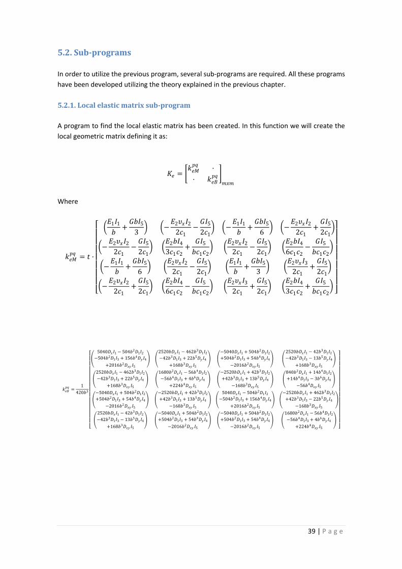
5.2.1. Local elastic matrix sub-program
A program to find the local elastic matrix has been created. In this function we will create the
local geometric matrix defining it as:
𝐾𝑒 = 𝑘𝑒𝑀𝑝𝑞
·
· 𝑘𝑒𝐵𝑝𝑞
𝑚𝑥𝑚
Where
𝑘𝑒𝑀𝑝𝑞
= 𝑡 ·
𝐸1𝐼1𝑏
+𝐺𝑏𝐼5
3 −
𝐸2𝜐𝑥𝐼22𝑐1
−𝐺𝐼52𝑐1
−𝐸1𝐼1𝑏
+𝐺𝑏𝐼5
6 −
𝐸2𝜐𝑥𝐼22𝑐1
+𝐺𝐼52𝑐1
−𝐸2𝜐𝑥𝐼2
2𝑐1−𝐺𝐼52𝑐1
𝐸2𝑏𝐼43𝑐1𝑐2
+𝐺𝐼5𝑏𝑐1𝑐2
𝐸2𝜐𝑥𝐼2
2𝑐1−𝐺𝐼52𝑐1
𝐸2𝑏𝐼46𝑐1𝑐2
−𝐺𝐼5𝑏𝑐1𝑐2
−𝐸1𝐼1𝑏
+𝐺𝑏𝐼5
6
𝐸2𝜐𝑥𝐼22𝑐1
−𝐺𝐼52𝑐1
𝐸1𝐼1𝑏
+𝐺𝑏𝐼5
3
𝐸2𝜐𝑥𝐼32𝑐1
+𝐺𝐼52𝑐1
−𝐸2𝜐𝑥𝐼2
2𝑐1+𝐺𝐼52𝑐1
𝐸2𝑏𝐼46𝑐1𝑐2
−𝐺𝐼5𝑏𝑐1𝑐2
𝐸2𝜐𝑥𝐼3
2𝑐1+𝐺𝐼52𝑐1
𝐸2𝑏𝐼43𝑐1𝑐2
+𝐺𝐼5𝑏𝑐1𝑐2
𝑘𝑒𝐵𝑝𝑞
=1
420𝑏3
5040𝐷𝑥𝐼1 − 504𝑏2𝐷1𝐼2−504𝑏2𝐷1𝐼3 + 156𝑏4𝐷𝑦𝐼4
+2016𝑏2𝐷𝑥𝑦 𝐼5
2520𝑏𝐷𝑥 𝐼1 − 462𝑏3𝐷1𝐼2−42𝑏3𝐷1𝐼3 + 22𝑏5𝐷𝑦𝐼4
+168𝑏3𝐷𝑥𝑦 𝐼5
−5040𝐷𝑥𝐼1 + 504𝑏2𝐷1𝐼2+504𝑏2𝐷1𝐼3 + 54𝑏4𝐷𝑦𝐼4
−2016𝑏2𝐷𝑥𝑦 𝐼5
2520𝑏𝐷𝑥𝐼1 − 42𝑏3𝐷1𝐼2−42𝑏3𝐷1𝐼3 − 13𝑏5𝐷𝑦𝐼4
+168𝑏3𝐷𝑥𝑦 𝐼5
2520𝑏𝐷𝑥𝐼1 − 462𝑏3𝐷1𝐼2−42𝑏3𝐷1𝐼3 + 22𝑏5𝐷𝑦𝐼4
+168𝑏3𝐷𝑥𝑦 𝐼5
1680𝑏2𝐷𝑥𝐼1 − 56𝑏4𝐷1𝐼2−56𝑏4𝐷1𝐼3 + 4𝑏6𝐷𝑦𝐼4
+224𝑏4𝐷𝑥𝑦 𝐼5
−2520𝑏𝐷𝑥𝐼1 + 42𝑏3𝐷1𝐼2+42𝑏3𝐷1𝐼3 + 13𝑏5𝐷𝑦𝐼4
−168𝑏3𝐷𝑥𝑦 𝐼5
840𝑏2𝐷𝑥𝐼1 + 14𝑏4𝐷1𝐼2+14𝑏4𝐷1𝐼3 − 3𝑏6𝐷𝑦𝐼4
−56𝑏4𝐷𝑥𝑦 𝐼5
−5040𝐷𝑥𝐼1 + 504𝑏2𝐷1𝐼2+504𝑏2𝐷1𝐼3 + 54𝑏4𝐷𝑦𝐼4
−2016𝑏2𝐷𝑥𝑦 𝐼5
−2520𝑏𝐷𝑥 𝐼1 + 42𝑏3𝐷1𝐼2+42𝑏3𝐷1𝐼3 + 13𝑏5𝐷𝑦𝐼4
−168𝑏3𝐷𝑥𝑦 𝐼5
5040𝐷𝑥𝐼1 − 504𝑏2𝐷1𝐼2−504𝑏2𝐷1𝐼3 + 156𝑏4𝐷𝑦𝐼4
+2016𝑏2𝐷𝑥𝑦 𝐼5
−2520𝑏𝐷𝑥𝐼1 + 462𝑏3𝐷1𝐼2+42𝑏3𝐷1𝐼3 − 22𝑏5𝐷𝑦𝐼4
−168𝑏3𝐷𝑥𝑦 𝐼5
2520𝑏𝐷𝑥𝐼1 − 42𝑏3𝐷1𝐼2−42𝑏3𝐷1𝐼3 − 13𝑏5𝐷𝑦𝐼4
+168𝑏3𝐷𝑥𝑦 𝐼5
−5040𝐷𝑥𝐼1 + 504𝑏2𝐷1𝐼2+504𝑏2𝐷1𝐼3 + 54𝑏4𝐷𝑦𝐼4
−2016𝑏2𝐷𝑥𝑦 𝐼5
−5040𝐷𝑥𝐼1 + 504𝑏2𝐷1𝐼2+504𝑏2𝐷1𝐼3 + 54𝑏4𝐷𝑦𝐼4
−2016𝑏2𝐷𝑥𝑦 𝐼5
1680𝑏2𝐷𝑥𝐼1 − 56𝑏4𝐷1𝐼2−56𝑏4𝐷1𝐼3 + 4𝑏6𝐷𝑦𝐼4
+224𝑏4𝐷𝑥𝑦 𝐼5

40 | P a g e
The program is named “k_elastic_local” and the function is:
function [k_elastic_local]=k_elastic_local(Ex,Ey,vx,vy,G,t,a,b,BC,m_a)
INPUTS OUTPUTS
Ex: Young modulus in the “x” direction. Ey: Young modulus in the “y” direction. vx: Poisson’s ratio in the “x” direction. vy: Poisson’s ratio in the “y” direction. G: Shear modulus for the material. t: Thickness of the analyzed strip element. a: Length of the strip element. b: Width of the strip element. BC: Boundary conditions of the loaded edges. m_a: Analyzed half-waves for the strip element.
k_elastic_local: The elastic stiffness matrix for the defined strip element in local coordinates.
5.2.2. Local geometric matrix sub-program
A program similar to the previous one has also been created to find the local geometric matrix.
In this function we will create the local geometric matrix defining it as:
𝐾𝑔 = 𝑘𝑔𝑀𝑝𝑞
·
· 𝑘𝑔𝐵𝑝𝑞
𝑚𝑥𝑚
Where:
𝑘𝑔𝑀𝑝𝑞
=
3𝑇1 + 𝑇2 𝑏𝐼5
120
𝑇1 + 𝑇2 𝑏𝐼512
0
0 3𝑇1 + 𝑇2 𝑏𝑎
2𝐼412𝜇𝑝𝜇𝑞
0 𝑇1 + 𝑇2 𝑏𝑎
2𝐼412𝜇𝑝𝜇𝑞
𝑇1 + 𝑇2 𝑏𝐼512
0 3𝑇1 + 𝑇2 𝑏𝐼5
120
0 𝑇1 + 𝑇2 𝑏𝑎
2𝐼412𝜇𝑝𝜇𝑞
0 3𝑇1 + 𝑇2 𝑏𝑎
2𝐼412𝜇𝑝𝜇𝑞
𝑘𝑔𝐵𝑝𝑞
=
10𝑇1 + 3𝑇2 𝑏𝐼5
35
15𝑇1 + 7𝑇2 𝑏2𝐼5
420
𝑇1 + 𝑇2 𝑏𝐼5140
− 7𝑇1 + 6𝑇2 𝑏
2𝐼5420
15𝑇1 + 7𝑇2 𝑏2𝐼5
420
5𝑇1 + 3𝑇2 𝑏3𝐼5
840
6𝑇1 + 7𝑇2 𝑏2𝐼5
420− 𝑇1 + 𝑇2 𝑏
3𝐼5280
𝑇1 + 𝑇2 𝑏𝐼5140
6𝑇1 + 7𝑇2 𝑏2𝐼5
420
3𝑇1 + 10𝑇2 𝑏𝐼535
− 7𝑇1 + 15𝑇2 𝑏
2𝐼5420
− 7𝑇1 + 6𝑇2 𝑏
2𝐼5420
− 𝑇1 + 𝑇2 𝑏
3𝐼5280
− 7𝑇1 + 15𝑇2 𝑏
2𝐼5420
3𝑇1 + 5𝑇2 𝑏3𝐼5
840
41 | P a g e
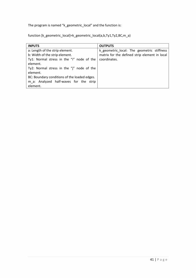
The program is named “k_geometric_local” and the function is:
function [k_geometric_local]=k_geometric_local(a,b,Ty1,Ty2,BC,m_a)
INPUTS OUTPUTS
a: Length of the strip element. b: Width of the strip element. Ty1: Normal stress in the “i” node of the element. Ty2: Normal stress in the “j” node of the element. BC: Boundary conditions of the loaded edges. m_a: Analyzed half-waves for the strip element.
k_geometric_local: The geometric stiffness matrix for the defined strip element in local coordinates.

42 | P a g e
5.2.3. Boundary conditions calculator
A function to calculate the five undetermined parameters I1, I2, I3, I4 and I5 for the local
elastic and geometric stiffness matrix has been created. The parameters are defined as:
𝐼1 = 𝑌𝑝 · 𝑌𝑞 · 𝑑𝑦𝑎
0
𝐼2 = 𝑌𝑝′′ · 𝑌𝑞 · 𝑑𝑦
𝑎
0
𝐼3 = 𝑌𝑝 · 𝑌𝑞′′ · 𝑑𝑦
𝑎
0
𝐼4 = 𝑌𝑝′′ · 𝑌𝑞
′′ · 𝑑𝑦𝑎
0
𝐼5 = 𝑌𝑝′ · 𝑌𝑞
′ · 𝑑𝑦𝑎
0
As we can see, the I values depend on the two half-waves we analyze “p” and “q”.
The program is called “BCparameters” and the function is:
function [I1,I2,I3,I4,I5] = BCparameters(BC,Nm,Np,a)
INPUTS OUTPUTS
BC: Boundary conditions as defined previously: 'S-S': Simply-simply supported
boundary condition at loaded edges. 'C-C': Clamped-clamped boundary
condition at loaded edges. 'S-C': Simply-clamped boundary
condition at loaded edges. 'C-F': Clamped-free supported
boundary condition at loaded edges. 'C-G': Clamped-guided supported
boundary condition at loaded edges. Nm: Half-wave number “q”. Np: Half-wave number “p”. a: Length of the analyzed strip element.
I1, I2, I3, I4, I5: Undetermined parameters utilized in the geometric and elastic local stiffness matrices. They depend on the half-waves number “p” and “q” which appear in the matrices:
𝑘𝑒𝑝𝑞
and 𝑘𝑔𝑝𝑞

43 | P a g e
5.2.4. Element properties
From the input elements we need to find a few parameters in order to use the other functions.
For this the “elemprop” function has been created and the function is:
function [elprop]=elemprop(node,elem,nnodes,nelems)
INPUTS OUTPUTS
node: The nodes as defined before: [node_numberx_positionz_position stress] elem: The elements as defined before: [element_numbernodeinodej t] nnodes and nelems: Number of nodes and elements in our section.
elprop: A variable including [element_numberwidth alpha] Where the “width” will be used for the local matrices and the “alpha” to change the local coordinates to global coordinates.
5.2.5. Rotation
This program is used to transform the local coordinate matrices to global coordinates. It
utilizes a matrix to rotate the strip. The rotation depends on the angle “𝛼”.
Figure 28: Strip rotation guide image
The program is called “rotatestrip” and the function is:
[k_elastic_global,k_geometric_global]=rotatestrip(alpha,k_elastic,k_geometric,m_a)
INPUTS OUTPUTS
alpha: angle “𝛼” for the strip as defined in the image. k_elastic: elastic matrix in local coordinates. k_geometric: geometric matrix in local coordinates. m_a: Analyzed half-waves for the strip element.
k_elastic_global: elastic matrix in global coordinates. k_geometric_global: geometric matrix in global coordinates.

44 | P a g e
5.2.6. Assembly
Another program has been used to join all the strips. Using the strips elastic and geometric
matrices in global coordinates, the function will join the particular strip to the full global
matrix. The program is called “assemble_elements” and the function is:
[K_elastic,K_geometric]=assemble_elements(K_elastic,K_geometric,k_elastic_local,k_geometri
c_local,nodei,nodej,nnodes,m_a)
INPUTS OUTPUTS
K_elastic: Full elastic matrix for the section. K_geometric: Full geometric matrix for the section. k_elastic_global: Elastic matrix for the strip in global coordinates. k_geometric_global: Geometric matrix for the strip in global coordinates. nodei and nodej: Nodes of the element. nnodes: Number of nodes in the section m_a: Analyzed half-waves for the strip element.
K_elastic: Full elastic matrix for the section adding the elastic matrix of the strip element defined by “k_elastic_global”. K_geometric: Full geometric matrix for the section adding the geometric matrix of the strip element defined by “k_geometric_global”.

45 | P a g e
5.3. Matlab function map
46 | P a g e
6. Comparison with other methods
In order to verify the usefulness of our program it is crucial that we compare the results we
obtain with other programs or theories that we know have the correct results. This way we can
compare both the error and the time difference with our program.
As previously stated, our method should be much quicker due to the fact that it has many less
freedom degrees than the Finite Element Method. However, we must verify that the error is
acceptable.
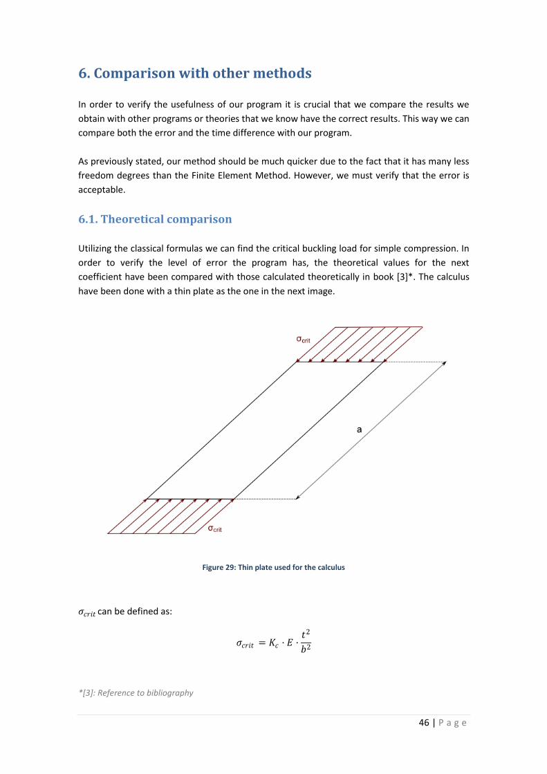
6.1. Theoretical comparison
Utilizing the classical formulas we can find the critical buckling load for simple compression. In
order to verify the level of error the program has, the theoretical values for the next
coefficient have been compared with those calculated theoretically in book [3]*. The calculus
have been done with a thin plate as the one in the next image.
Figure 29: Thin plate used for the calculus
𝜎𝑐𝑟𝑖𝑡 can be defined as:
𝜎𝑐𝑟𝑖𝑡 = 𝐾𝑐 · 𝐸 ·𝑡2
𝑏2
*[3]: Reference to bibliography

47 | P a g e
Where:
o 𝐾𝑐 is a coefficient that depends on the boundary conditions and on the relation
between the length and width of the plate.
o 𝐸is the Young modulus.
o 𝑡is the thickness of the plate.
o 𝑏is the width of the plate.
o 𝑎is the length of the plate.
In order to find the values for K we must create a thin plate problem. In our case we will do it
with 10 nodes in the transversal direction. The complete exercise is added in the annexes. In
the next table we will see the results.
𝒂
𝒃
Boundary conditions
Simply-Simply Clamped-Clamped
Theoretical K FSM program K Difference Theoretical K FSM program K Difference
𝟎,𝟓 3,5 3,518 0,5% 15,8 14,347 9,2%
𝟎,𝟔 2,5 2,432 2,7% 10 9,949 0,5%
𝟎,𝟕 1,8 1,778 1,2% 7,3 7,300 0%
𝟎,𝟗 1,2 1,067 11,1% 4,5 4,405 2,1%
𝟏,𝟎 0,9 0,861 4,3% 3,7 3,564 3,7%
𝟏,𝟐 0,7 0,594 15,1% 2,5 2,469 1,2%
𝟏,𝟒 0,5 0,434 13,2% 1,8 1,811 0,6%
𝟏,𝟖 0,25 0,260 4% 1,15 1,090 5,2%
𝟐,𝟎 0,2 0,209 4,5% 0,9 0,884 1,8%
𝟐,𝟒 0,15 0,145 3,3% 0,6 0,613 2,2%
> 𝟑 0,1 0,092 8% 0,4 0,391 2,3%
We can see that the differences between both calculi are small enough. The differences
between the values come due to the different formulation between the semi-analytical
method and the FSM.

48 | P a g e
6.2. Finite Element Method Comparison
As previously stated, the Finite Element Method gives a more accurate result than the Finite
Strip Method, although it demands much more computer capacity and time.
In order to calibrate the accuracy of the FSM program the values obtained with FEM are
utilized and compared to calibrate the program. Values obtained from the article [6]* are
utilized in the following comparison.
The whole comparison exercise can be found in the annexes. Here we will only look at the
results.
Section 𝜎𝑐𝑟𝑖𝑡 Error a=100, b=110, h=170,
lip length=30 Finite strip method Finite element method
t=1 mm 37,99 37,74 0,66%
t=2 mm 151,85 150,52 0,88%
t=3 mm 341,29 337,07 1,24%
t=4 mm 605,86 595,36 1,73%
t=5 mm 944,85 922,69 2,35%
Degrees of freedom 17 nodes * 4 dof = 68 degrees of freedom
17 nodes in the section * 5 nodes in the longitudinal
direction * 4 dof = 340 degrees of freedom
We can see therefore that the error percentage is very small and acceptable.
The small error that we can find is due to the fact that the finite element method does
implement the shear strains into its calculus, while de finite strip method follows the Kirchhoff
theory, where the shear strains are not taken into account because they are extremely small.
*[6]: Reference to bibliography

49 | P a g e
7. Conclusions
The objective of this project was to develop a program capable of implementing the FSM
theory in order to solve structural problems. The new formulation of the FSM with the theories
of Kirchhoff and Reissner-Mindlin for the analysis of rectangular structures is implemented to
the program.
The results are well calibrated in comparison to those in the plate theory. Regarding FEM, the
solutions are comparatively quite correct, with a small difference in the buckling critical
coefficient of about 1%. This small error is due to the fact that FEM solutions include shear
strain effects while the FSM solution does not.
Therefore, we can extract some conclusions:
o The Finite Strip Method, although being a semi-analytical theory that utilizes
trigonometric Fourier series in the longitudinal direction and FEM in the transversal
direction, can be correctly utilized to solve a rectangular problem with various
sections.
o The dimension of the problem is greatly reduced with FSM. It is reduced to a system
with two middle nodes with four displacements each. Thanks to the Fourier series, we
can define the boundary conditions with trigonometric functions that satisfy them in
the loaded edges.
o The boundary conditions are extremely important to determine the stiffness matrices
in the FSM, given that changing them will cause some coefficients inside the matrix to
vary.
o The behavior of our program is acceptable in many cases and much quicker than the
FEM solution to the same problem. The requirements for the computer are greatly
decreased because the unknowns in the problem are much lesser than in the finite
element method.

50 | P a g e
8. Further work
Having finished the finite strip method, there are several new things that could be done in
order to continue with this investigation.
The program that has been developed only solves a single column. It would be interesting to
solve a whole frame utilizing the finite strip method in every column separately. However, in
order to do this, further investigation must be made in the unions between the bars. In the
next image we can see an illustration of what the next objective could be:
Figure 30: Frame
Although all the bars can correctly be analyzed by the Finite Strip Method when taking them
separately, it requires further analysis to know if it is possible to solve a complete frame
utilizing this method.
51 | P a g e
9. Bibliography
1. OÑATE, Eugenio: “Cálculo de Estructuras por el Método de los Elementos Finitos”,
2. JOVICEVIC, J and OÑATE, E: “Analisis of Beams and Shells Using a Rotation”
3. GÉMINARD, Lucien and GIET, Armand: “Stabilité des constructions”
4. Y. K. Cheung, L. G. Tham, “The Finite Strip Method”
5. LI, Z. and SCHAFER, B.W. (2010) “Buckling analysis of cold-formed steel members with
general boundary conditions using CUFSM: conventional and constrained finite strip
methods.” Proceedings of the 20th Int;l. Spec. Conf. on Cold-Formed Steel Structures,
St. Louis, MO. November, 2010.
6. BUI HUNG CUONG, “Analysestatique du comportement des structures a parois minces
par la method des elements finis et des bandesfinies de type plaque et
coquesurbaisseedeformables en cisaiilement”
7. TIMOSHENKO – GOUDIER, “Theory of Elasticity”
Special thanks
To Professor SélimDatoussaïd, for being so understanding with my initial little knowledge of
Finite Element Method and helping me a lot during the whole project.
To Professor Ben Schafer’s thin-walled structures research group, for creating the marvelous
program CUFSM 4.05, which has been extremely helpful, together with all the theory behind it,
with this project.
52 | P a g e
Annex
1. Matlab programs
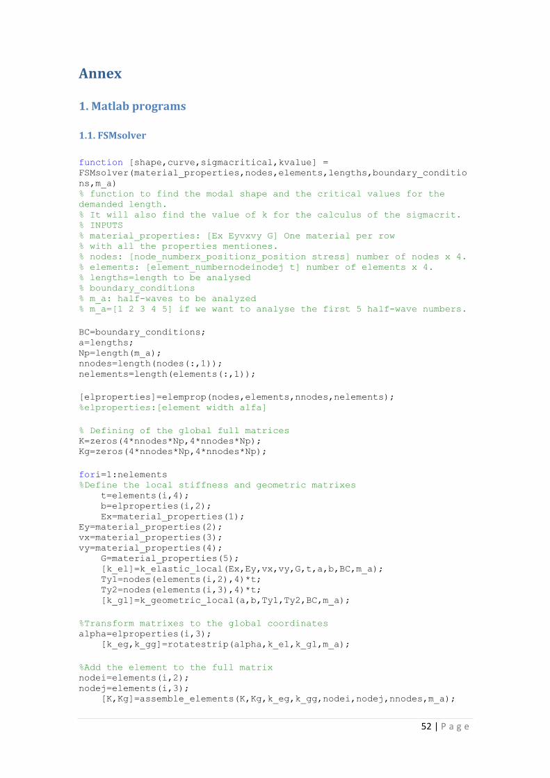
1.1. FSMsolver
function [shape,curve,sigmacritical,kvalue] =
FSMsolver(material_properties,nodes,elements,lengths,boundary_conditio
ns,m_a) % function to find the modal shape and the critical values for the
demanded length. % It will also find the value of k for the calculus of the sigmacrit. % INPUTS % material_properties: [Ex Eyvxvy G] One material per row % with all the properties mentiones. % nodes: [node_numberx_positionz_position stress] number of nodes x 4. % elements: [element_numbernodeinodej t] number of elements x 4. % lengths=length to be analysed % boundary_conditions % m_a: half-waves to be analyzed % m_a=[1 2 3 4 5] if we want to analyse the first 5 half-wave numbers.
BC=boundary_conditions; a=lengths; Np=length(m_a); nnodes=length(nodes(:,1)); nelements=length(elements(:,1));
[elproperties]=elemprop(nodes,elements,nnodes,nelements); %elproperties:[element width alfa]
% Defining of the global full matrices K=zeros(4*nnodes*Np,4*nnodes*Np); Kg=zeros(4*nnodes*Np,4*nnodes*Np);
fori=1:nelements %Define the local stiffness and geometric matrixes t=elements(i,4); b=elproperties(i,2); Ex=material_properties(1); Ey=material_properties(2); vx=material_properties(3); vy=material_properties(4); G=material_properties(5); [k_el]=k_elastic_local(Ex,Ey,vx,vy,G,t,a,b,BC,m_a); Ty1=nodes(elements(i,2),4)*t; Ty2=nodes(elements(i,3),4)*t; [k_gl]=k_geometric_local(a,b,Ty1,Ty2,BC,m_a);
%Transform matrixes to the global coordinates alpha=elproperties(i,3); [k_eg,k_gg]=rotatestrip(alpha,k_el,k_gl,m_a);
%Add the element to the full matrix nodei=elements(i,2); nodej=elements(i,3); [K,Kg]=assemble_elements(K,Kg,k_eg,k_gg,nodei,nodej,nnodes,m_a);

53 | P a g e
end
R=eye(4*nnodes*Np); Kff=R'*K*R; Kffg=R'*Kg*R;
%function eig: returs [V,D] so K*V=D*Kg*V where D is a diagonal matrix
with %the values of the critical buckling forces in the diagonal. neigs=10; options.disp=0; options.issym=1; N=max(min(2*neigs,length(Kff(1,:))),1); [V,D]=eigs(full(Kffg\Kff),N,'SM',options); curve=diag(D); shape=V;
%The critical mode will be that one with the smallest critical value sigmacritical=min(curve); b=90; kvalue=sigmacritical*b^2/(Ex*t^2); end
1.2. K_elastic_local
function [k_elastic_local]=k_elastic_local(Ex,Ey,vx,vy,G,t,a,b,BC,m_a) % %Create the elastic stiffness matrix in global coordinates
% Inputs: % Ex,Ey,vx,vy,G: material properties % t: thickness of the element % a: length of the strip (longitudinal) % b: width of the strip (tranversal) % BC: ['S-S'] a string specifying boundary conditions to be analyzed: %'S-S' simply-simply supported boundary condition %'C-C' clamped-clamped boundary condition %'S-C' simply-clamped supported boundary condition %'C-F' clamped-free supported boundary condition %'C-G' clamped-guided supported boundary condition % m_a: longitudinal terms (or half-wave numbers) for this length. % m_a=[1 2 3 4 5] if we want to analyse the first 5 half-wave numbers.
% Output: % k: local stiffness matrix, a totalm x totalm matrix of 8 by 8
submatrices. % k=[kmp]totalm x totalm block matrix % each kmp is the 8 x 8 submatrix in the DOF order [u1 v1 u2 v2 w1
theta1 w2 theta2]';
E1=Ex/(1-vx*vy); E2=Ey/(1-vx*vy); Dx=Ex*t^3/(12*(1-vx*vy)); Dy=Ey*t^3/(12*(1-vx*vy)); D1=vx*Ey*t^3/(12*(1-vx*vy)); Dxy=G*t^3/12; % totalm = length(m_a); %Total number of longitudinal terms m %

54 | P a g e
k_elastic_local=sparse(zeros(8*totalm,8*totalm)); z0=zeros(4,4); for m=1:1:totalm for p=1:1:totalm % km_mp=zeros(4,4); kf_mp=zeros(4,4); um=m_a(m)*pi; up=m_a(p)*pi; c1=um/a; c2=up/a; % [I1,I2,I3,I4,I5] = BCparameters(BC,m_a(m),m_a(p),a); % %asemble the matrix of Km_mp (K membrane for m and p half-waves) km_mp(1,1)=E1*I1/b+G*b*I5/3; km_mp(1,2)=E2*vx*(-1/2/c2)*I3-G*I5/2/c2; km_mp(1,3)=-E1*I1/b+G*b*I5/6; km_mp(1,4)=E2*vx*(-1/2/c2)*I3+G*I5/2/c2;
km_mp(2,1)=E2*vx*(-1/2/c1)*I2-G*I5/2/c1; km_mp(2,2)=E2*b*I4/3/c1/c2+G*I5/b/c1/c2; km_mp(2,3)=E2*vx*(1/2/c1)*I2-G*I5/2/c1; km_mp(2,4)=E2*b*I4/6/c1/c2-G*I5/b/c1/c2;
km_mp(3,1)=-E1*I1/b+G*b*I5/6; km_mp(3,2)=E2*vx*(1/2/c2)*I3-G*I5/2/c2; km_mp(3,3)=E1*I1/b+G*b*I5/3; km_mp(3,4)=E2*vx*(1/2/c2)*I3+G*I5/2/c2;
km_mp(4,1)=E2*vx*(-1/2/c1)*I2+G*I5/2/c1; km_mp(4,2)=E2*b*I4/6/c1/c2-G*I5/b/c1/c2; km_mp(4,3)=E2*vx*(1/2/c1)*I2+G*I5/2/c1; km_mp(4,4)=E2*b*I4/3/c1/c2+G*I5/b/c1/c2; km_mp=km_mp*t; % % %asemble the matrix of Kf_mp (K bending for m and p half-waves) kf_mp(1,1)=(5040*Dx*I1-504*b^2*D1*I2-
504*b^2*D1*I3+156*b^4*Dy*I4+2016*b^2*Dxy*I5)/420/b^3; kf_mp(1,2)=(2520*b*Dx*I1-462*b^3*D1*I2-
42*b^3*D1*I3+22*b^5*Dy*I4+168*b^3*Dxy*I5)/420/b^3; kf_mp(1,3)=(-
5040*Dx*I1+504*b^2*D1*I2+504*b^2*D1*I3+54*b^4*Dy*I4-
2016*b^2*Dxy*I5)/420/b^3; kf_mp(1,4)=(2520*b*Dx*I1-42*b^3*D1*I2-42*b^3*D1*I3-
13*b^5*Dy*I4+168*b^3*Dxy*I5)/420/b^3;
kf_mp(2,1)=(2520*b*Dx*I1-462*b^3*D1*I3-
42*b^3*D1*I2+22*b^5*Dy*I4+168*b^3*Dxy*I5)/420/b^3; kf_mp(2,2)=(1680*b^2*Dx*I1-56*b^4*D1*I2-
56*b^4*D1*I3+4*b^6*Dy*I4+224*b^4*Dxy*I5)/420/b^3; kf_mp(2,3)=(-
2520*b*Dx*I1+42*b^3*D1*I2+42*b^3*D1*I3+13*b^5*Dy*I4-
168*b^3*Dxy*I5)/420/b^3; kf_mp(2,4)=(840*b^2*Dx*I1+14*b^4*D1*I2+14*b^4*D1*I3-
3*b^6*Dy*I4-56*b^4*Dxy*I5)/420/b^3;
kf_mp(3,1)=kf_mp(1,3); kf_mp(3,2)=kf_mp(2,3);

55 | P a g e
kf_mp(3,3)=(5040*Dx*I1-504*b^2*D1*I2-
504*b^2*D1*I3+156*b^4*Dy*I4+2016*b^2*Dxy*I5)/420/b^3; kf_mp(3,4)=(-2520*b*Dx*I1+462*b^3*D1*I2+42*b^3*D1*I3-
22*b^5*Dy*I4-168*b^3*Dxy*I5)/420/b^3;
kf_mp(4,1)=kf_mp(1,4); kf_mp(4,2)=kf_mp(2,4); kf_mp(4,3)=(-2520*b*Dx*I1+462*b^3*D1*I3+42*b^3*D1*I2-
22*b^5*Dy*I4-168*b^3*Dxy*I5)/420/b^3;%not symmetric kf_mp(4,4)=(1680*b^2*Dx*I1-56*b^4*D1*I2-
56*b^4*D1*I3+4*b^6*Dy*I4+224*b^4*Dxy*I5)/420/b^3;
%assemble the membrane and bending stiffness matrices kmp=[km_mp z0 z0 kf_mp]; %add it into local element stiffness matrix by corresponding to half-
wave m k_elastic_local(8*(m-1)+1:8*m,8*(p-1)+1:8*p)=kmp; end end
1.3. K_geometric_local
function [k_geometric_local]=k_geometric_local(a,b,Ty1,Ty2,BC,m_a) % %Generate geometric stiffness matrix (kg) in local coordinates
% Inputs: % a: length of the strip in longitudinal direction % b: width of the strip in transverse direction % Ty1, Ty2: node stresses % BC: a string specifying boundary conditions to be analyzed: %'S-S' simply-pimply supported boundary condition at loaded edges %'C-C' clamped-clamped boundary condition at loaded edges %'S-C' simply-clamped supported boundary condition at loaded edges %'C-F' clamped-free supported boundary condition at loaded edges %'C-G' clamped-guided supported boundary condition at loaded edges % m_a: longitudinal terms (or half-wave numbers) for this length. % m_a=[1 2 3 4 5] if we want to analyse the first 5 half-wave numbers.
% Output: % kg: local geometric stiffness matrix, a totalm x totalm matrix of 8
by 8 submatrices. % kg=[kgmp]totalm x totalm block matrix % each kgmp is the 8 x 8 submatrix in the DOF order [u1 v1 u2 v2 w1
theta1 % w2 theta2]';
totalm = length(m_a); %Total number of longitudinal terms m kg=sparse(zeros(8*totalm,8*totalm)); % for m=1:1:totalm for p=1:1:totalm % gm_mp=zeros(4,4); z0=zeros(4,4); gf_mp=zeros(4,4); um=m_a(m)*pi; up=m_a(p)*pi;
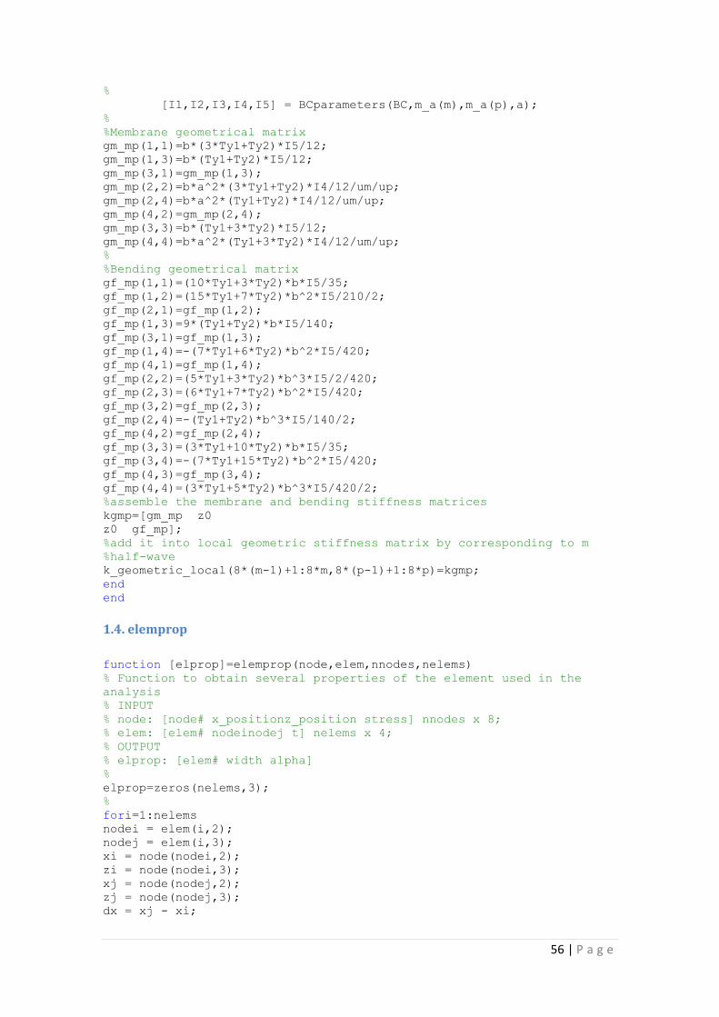
56 | P a g e
% [I1,I2,I3,I4,I5] = BCparameters(BC,m_a(m),m_a(p),a); % %Membrane geometrical matrix gm_mp(1,1)=b*(3*Ty1+Ty2)*I5/12; gm_mp(1,3)=b*(Ty1+Ty2)*I5/12; gm_mp(3,1)=gm_mp(1,3); gm_mp(2,2)=b*a^2*(3*Ty1+Ty2)*I4/12/um/up; gm_mp(2,4)=b*a^2*(Ty1+Ty2)*I4/12/um/up; gm_mp(4,2)=gm_mp(2,4); gm_mp(3,3)=b*(Ty1+3*Ty2)*I5/12; gm_mp(4,4)=b*a^2*(Ty1+3*Ty2)*I4/12/um/up; % %Bending geometrical matrix gf_mp(1,1)=(10*Ty1+3*Ty2)*b*I5/35; gf_mp(1,2)=(15*Ty1+7*Ty2)*b^2*I5/210/2; gf_mp(2,1)=gf_mp(1,2); gf_mp(1,3)=9*(Ty1+Ty2)*b*I5/140; gf_mp(3,1)=gf_mp(1,3); gf_mp(1,4)=-(7*Ty1+6*Ty2)*b^2*I5/420; gf_mp(4,1)=gf_mp(1,4); gf_mp(2,2)=(5*Ty1+3*Ty2)*b^3*I5/2/420; gf_mp(2,3)=(6*Ty1+7*Ty2)*b^2*I5/420; gf_mp(3,2)=gf_mp(2,3); gf_mp(2,4)=-(Ty1+Ty2)*b^3*I5/140/2; gf_mp(4,2)=gf_mp(2,4); gf_mp(3,3)=(3*Ty1+10*Ty2)*b*I5/35; gf_mp(3,4)=-(7*Ty1+15*Ty2)*b^2*I5/420; gf_mp(4,3)=gf_mp(3,4); gf_mp(4,4)=(3*Ty1+5*Ty2)*b^3*I5/420/2; %assemble the membrane and bending stiffness matrices kgmp=[gm_mp z0 z0 gf_mp]; %add it into local geometric stiffness matrix by corresponding to m %half-wave k_geometric_local(8*(m-1)+1:8*m,8*(p-1)+1:8*p)=kgmp; end end
1.4. elemprop
function [elprop]=elemprop(node,elem,nnodes,nelems) % Function to obtain several properties of the element used in the
analysis % INPUT % node: [node# x_positionz_position stress] nnodes x 8; % elem: [elem# nodeinodej t] nelems x 4; % OUTPUT % elprop: [elem# width alpha] % elprop=zeros(nelems,3); % fori=1:nelems nodei = elem(i,2); nodej = elem(i,3); xi = node(nodei,2); zi = node(nodei,3); xj = node(nodej,2); zj = node(nodej,3); dx = xj - xi;

57 | P a g e
dz = zj - zi; width = sqrt(dx^2 + dz^2); alpha = atan2(dz,dx); elprop(i,:)=[i width alpha]; end
1.5. BCparameters
function [I1,I2,I3,I4,I5] = BCparameters(BC,Nm,Np,a) % % Calculate the 5 undetermined parameters I1,I2,I3,I4,I5 for local
elastic % and geometric stiffness matrices. % BC: a string specifying boundary conditions to be analyzed: %'S-S' simply-pimply supported boundary condition at loaded edges %'C-C' clamped-clamped boundary condition at loaded edges %'S-C' simply-clamped supported boundary condition at loaded edges %'C-F' clamped-free supported boundary condition at loaded edges %'C-G' clamped-guided supported boundary condition at loaded edges %Outputs: %I1,I2,I3,I4,I5 %calculation of I1 is the integration of Ym*Yn from 0 to a %calculation of I2 is the integration of Ym''*Yn from 0 to a %calculation of I3 is the integration of Ym*Yn'' from 0 to a %calculation of I3 is the integration of Ym*Yn'' from 0 to a %calculation of I4 is the integration of Ym''*Yn'' from 0 to a %calculation of I5 is the integration of Ym'*Yn' from 0 to a
ifstrcmp(BC,'S-S') %For simply-pimply supported boundary condition at loaded edges if Nm==Np I1=a/2; I2=-Nm^2*pi^2/a/2; I3=-Np^2*pi^2/a/2; I4=pi^4*Nm^4/2/a^3; I5=pi^2*Nm^2/2/a; else I1=0; I2=0; I3=0; I4=0; I5=0; end elseifstrcmp(BC,'C-C') %For Clamped-clamped boundary condition at loaded edges if Nm==Np if Nm==1 I1=3*a/8; else I1=a/4; end I2=-(Nm^2+1)*pi^2/4/a; I3=-(Np^2+1)*pi^2/4/a; I4=pi^4*((Nm^2+1)^2+4*Nm^2)/4/a^3; I5=(1+Nm^2)*pi^2/4/a; else if Nm-Np==2 I1=-a/8; I2=(Nm^2+1)*pi^2/8/a-Nm*pi^2/4/a; I3=(Np^2+1)*pi^2/8/a+Np*pi^2/4/a;

58 | P a g e
I4=-(Nm-1)^2*(Np+1)^2*pi^4/8/a^3; I5=-(1+Nm*Np)*pi^2/8/a; elseif Nm-Np==-2 I1=-a/8; I2=(Nm^2+1)*pi^2/8/a+Nm*pi^2/4/a; I3=(Np^2+1)*pi^2/8/a-Np*pi^2/4/a; I4=-(Nm+1)^2*(Np-1)^2*pi^4/8/a^3; I5=-(1+Nm*Np)*pi^2/8/a; else I1=0; I2=0; I3=0; I4=0; I5=0; end end elseifstrcmp(BC,'S-C') %For simply-clamped supported boundary condition at loaded edges if Nm==Np I1=(1+(Nm+1)^2/Nm^2)*a/2; I2=-(Nm+1)^2*pi^2/a; I3=-(Nm+1)^2*pi^2/a; I4=(Nm+1)^2*pi^4*((Nm+1)^2+Nm^2)/2/a^3; I5=(1+Nm)^2*pi^2/a; else if Nm-Np==1 I1=(Nm+1)*a/2/Nm; I2=-(Nm+1)*Nm*pi^2/2/a; I3=-(Np+1)^2*pi^2*(Nm+1)/2/a/Nm; I4=(Nm+1)*Nm*(Np+1)^2*pi^4/2/a^3; I5=(1+Nm)*(1+Np)*pi^2/2/a; elseif Nm-Np==-1 I1=(Np+1)*a/2/Np; I2=-(Nm+1)^2*pi^2*(Np+1)/2/a/Np; I3=-(Np+1)*Np*pi^2/2/a; I4=(Nm+1)^2*Np*(Np+1)*pi^4/2/a^3; I5=(1+Nm)*(1+Np)*pi^2/2/a; else I1=0; I2=0; I3=0; I4=0; I5=0; end end % elseifstrcmp(BC,'C-F') %For clamped-free supported boundary condition at loaded edges if Nm==Np I1=3*a/2-2*a*(-1)^(Nm-1)/(Nm-1/2)/pi; I2=(Nm-1/2)^2*pi^2*((-1)^(Nm-1)/(Nm-1/2)/pi-1/2)/a; I3=(Np-1/2)^2*pi^2*((-1)^(Np-1)/(Np-1/2)/pi-1/2)/a; I4=(Nm-1/2)^4*pi^4/2/a^3; I5=(Nm-1/2)^2*pi^2/2/a; else I1=a-a*(-1)^(Nm-1)/(Nm-1/2)/pi-a*(-1)^(Np-1)/(Np-1/2)/pi; I2=(Nm-1/2)^2*pi^2*((-1)^(Nm-1)/(Nm-1/2)/pi)/a; I3=(Np-1/2)^2*pi^2*((-1)^(Np-1)/(Np-1/2)/pi)/a; I4=0; I5=0; end

59 | P a g e
elseifstrcmp(BC,'C-G') %For clamped-guided supported boundary condition at loaded edges if Nm==Np if Nm==1 I1=3*a/8; else I1=a/4; end I2=-((Nm-1/2)^2+1/4)*pi^2/a/4; I3=-((Nm-1/2)^2+1/4)*pi^2/a/4; I4=((Nm-1/2)^2+1/4)^2*pi^4/4/a^3+(Nm-1/2)^2*pi^4/4/a^3; I5=(Nm-1/2)^2*pi^2/a/4+pi^2/16/a; else if Nm-Np==1 I1=-a/8; I2=((Nm-1/2)^2+1/4)*pi^2/a/8-(Nm-1/2)*pi^2/a/8; I3=((Np-1/2)^2+1/4)*pi^2/a/8+(Np-1/2)*pi^2/a/8; I4=-Np^4*pi^4/8/a^3; I5=-Np^2*pi^2/8/a; elseif Nm-Np==-1 I1=-a/8; I2=((Nm-1/2)^2+1/4)*pi^2/a/8+(Nm-1/2)*pi^2/a/8; I3=((Np-1/2)^2+1/4)*pi^2/a/8-(Np-1/2)*pi^2/a/8; I4=-Nm^4*pi^4/8/a^3; I5=-Nm^2*pi^2/8/a; else I1=0; I2=0; I3=0; I4=0; I5=0; end end end
1.6. rotatestrip
function
[k_elastic_global,k_geometric_global]=rotatestrip(alpha,k_elastic,k_ge
ometric,m_a)
% Transfer the local stiffness matrix into the global coordinates % OUTPUT % k_elastic_global: k_elastic input in global coordinates (rotating
input angle alpha) % k_geometric_global: k_geometric input in global coordinates
(rotating input angle alpha) % INPUT % k_elastic and k_geometric: local matrices that must be changed to
global coordinates % alpha: angle for turning matrices to the global coordinates % m_a: half-wave numbers to be analysed % m_a=[1 2 3 4 5] if we want to analyse the first 5 half-wave numbers.
totalm = length(m_a); %Total number of longitudinal terms m a=alpha; % z0=0; gam=[cos(a) z0 z0z0 -sin(a) z0 z0z0 z0 1 z0 z0z0z0z0z0

60 | P a g e
z0 z0cos(a) z0 z0z0 -sin(a) z0 z0 z0z0 1 z0 z0z0z0 sin(a) z0 z0z0cos(a) z0 z0z0 z0 z0z0z0z0 1 z0 z0 z0 z0 sin(a) z0 z0z0cos(a) z0 z0 z0z0z0z0z0z01 ]; %extend to multi-m fori=1:totalm gamma(8*(i-1)+1:8*i,8*(i-1)+1:8*i)=gam; end % k_elastic_global=gamma*k_elastic*gamma'; k_geometric_global=gamma*k_geometric*gamma'; end
1.7. assemble_elements
function
[K_elastic,K_geometric]=assemble_elements(K_elastic,K_geometric,k_elas
tic_global,k_geometric_global,nodei,nodej,nnodes,m_a) % % This function adds the local matrices to the global matrices. % INPUT % K_elastic: full elastic stiffness matrix without the local input % K_geometric: full geometric stiffness matrix without the local input % k_elastic_global: global coordinates elastic stiffness matrix to be
added % k_geometric_global: global coordinates geometric stiffness matrix to
be added % nodei: one of the nodes of the analysed strip element % nodej: the other node of the analysed strip element % nnodes: number of total node in out section % m_a: half-waves analysed. m_a=[1 2 3 4 5] if we want to analyse the
first 5 half-waves
% OUTPUTS % K_elastic: full elastic stiffness matrix with the added input
elastic matrix % K_geometric: full geometric stiffness matrix with the added input
geometric matrix
totalm = length(m_a); %Total number of half-wave terms m K2=sparse(zeros(4*nnodes*totalm,4*nnodes*totalm)); K3=sparse(zeros(4*nnodes*totalm,4*nnodes*totalm)); skip=2*nnodes; fori=1:1:totalm for j=1:1:totalm %Submatrices for the initial elastic stiffness k11=k_elastic_global(8*(i-1)+1:8*(i-1)+2,8*(j-1)+1:8*(j-1)+2); k12=k_elastic_global(8*(i-1)+1:8*(i-1)+2,8*(j-1)+3:8*(j-1)+4); k13=k_elastic_global(8*(i-1)+1:8*(i-1)+2,8*(j-1)+5:8*(j-1)+6); k14=k_elastic_global(8*(i-1)+1:8*(i-1)+2,8*(j-1)+7:8*(j-1)+8); k21=k_elastic_global(8*(i-1)+3:8*(i-1)+4,8*(j-1)+1:8*(j-1)+2); k22=k_elastic_global(8*(i-1)+3:8*(i-1)+4,8*(j-1)+3:8*(j-1)+4); k23=k_elastic_global(8*(i-1)+3:8*(i-1)+4,8*(j-1)+5:8*(j-1)+6); k24=k_elastic_global(8*(i-1)+3:8*(i-1)+4,8*(j-1)+7:8*(j-1)+8); k31=k_elastic_global(8*(i-1)+5:8*(i-1)+6,8*(j-1)+1:8*(j-1)+2); k32=k_elastic_global(8*(i-1)+5:8*(i-1)+6,8*(j-1)+3:8*(j-1)+4); k33=k_elastic_global(8*(i-1)+5:8*(i-1)+6,8*(j-1)+5:8*(j-1)+6); k34=k_elastic_global(8*(i-1)+5:8*(i-1)+6,8*(j-1)+7:8*(j-1)+8);

61 | P a g e
k41=k_elastic_global(8*(i-1)+7:8*(i-1)+8,8*(j-1)+1:8*(j-1)+2); k42=k_elastic_global(8*(i-1)+7:8*(i-1)+8,8*(j-1)+3:8*(j-1)+4); k43=k_elastic_global(8*(i-1)+7:8*(i-1)+8,8*(j-1)+5:8*(j-1)+6); k44=k_elastic_global(8*(i-1)+7:8*(i-1)+8,8*(j-1)+7:8*(j-1)+8); % K2(4*nnodes*(i-1)+nodei*2-1:4*nnodes*(i-1)+nodei*2,4*nnodes*(j-
1)+nodei*2-1:4*nnodes*(j-1)+nodei*2)=k11; K2(4*nnodes*(i-1)+nodei*2-1:4*nnodes*(i-1)+nodei*2,4*nnodes*(j-
1)+nodej*2-1:4*nnodes*(j-1)+nodej*2)=k12; K2(4*nnodes*(i-1)+nodej*2-1:4*nnodes*(i-1)+nodej*2,4*nnodes*(j-
1)+nodei*2-1:4*nnodes*(j-1)+nodei*2)=k21; K2(4*nnodes*(i-1)+nodej*2-1:4*nnodes*(i-1)+nodej*2,4*nnodes*(j-
1)+nodej*2-1:4*nnodes*(j-1)+nodej*2)=k22; % K2(4*nnodes*(i-1)+skip+nodei*2-1:4*nnodes*(i-
1)+skip+nodei*2,4*nnodes*(j-1)+skip+nodei*2-1:4*nnodes*(j-
1)+skip+nodei*2)=k33; K2(4*nnodes*(i-1)+skip+nodei*2-1:4*nnodes*(i-
1)+skip+nodei*2,4*nnodes*(j-1)+skip+nodej*2-1:4*nnodes*(j-
1)+skip+nodej*2)=k34; K2(4*nnodes*(i-1)+skip+nodej*2-1:4*nnodes*(i-
1)+skip+nodej*2,4*nnodes*(j-1)+skip+nodei*2-1:4*nnodes*(j-
1)+skip+nodei*2)=k43; K2(4*nnodes*(i-1)+skip+nodej*2-1:4*nnodes*(i-
1)+skip+nodej*2,4*nnodes*(j-1)+skip+nodej*2-1:4*nnodes*(j-
1)+skip+nodej*2)=k44; % K2(4*nnodes*(i-1)+nodei*2-1:4*nnodes*(i-1)+nodei*2,4*nnodes*(j-
1)+skip+nodei*2-1:4*nnodes*(j-1)+skip+nodei*2)=k13; K2(4*nnodes*(i-1)+nodei*2-1:4*nnodes*(i-1)+nodei*2,4*nnodes*(j-
1)+skip+nodej*2-1:4*nnodes*(j-1)+skip+nodej*2)=k14; K2(4*nnodes*(i-1)+nodej*2-1:4*nnodes*(i-1)+nodej*2,4*nnodes*(j-
1)+skip+nodei*2-1:4*nnodes*(j-1)+skip+nodei*2)=k23; K2(4*nnodes*(i-1)+nodej*2-1:4*nnodes*(i-1)+nodej*2,4*nnodes*(j-
1)+skip+nodej*2-1:4*nnodes*(j-1)+skip+nodej*2)=k24; % K2(4*nnodes*(i-1)+skip+nodei*2-1:4*nnodes*(i-
1)+skip+nodei*2,4*nnodes*(j-1)+nodei*2-1:4*nnodes*(j-1)+nodei*2)=k31; K2(4*nnodes*(i-1)+skip+nodei*2-1:4*nnodes*(i-
1)+skip+nodei*2,4*nnodes*(j-1)+nodej*2-1:4*nnodes*(j-1)+nodej*2)=k32; K2(4*nnodes*(i-1)+skip+nodej*2-1:4*nnodes*(i-
1)+skip+nodej*2,4*nnodes*(j-1)+nodei*2-1:4*nnodes*(j-1)+nodei*2)=k41; K2(4*nnodes*(i-1)+skip+nodej*2-1:4*nnodes*(i-
1)+skip+nodej*2,4*nnodes*(j-1)+nodej*2-1:4*nnodes*(j-1)+nodej*2)=k42; % %Submatrices for the initial geometric stiffness kg11=k_geometric_global(8*(i-1)+1:8*(i-1)+2,8*(j-1)+1:8*(j-
1)+2); kg12=k_geometric_global(8*(i-1)+1:8*(i-1)+2,8*(j-1)+3:8*(j-
1)+4); kg13=k_geometric_global(8*(i-1)+1:8*(i-1)+2,8*(j-1)+5:8*(j-
1)+6); kg14=k_geometric_global(8*(i-1)+1:8*(i-1)+2,8*(j-1)+7:8*(j-
1)+8); kg21=k_geometric_global(8*(i-1)+3:8*(i-1)+4,8*(j-1)+1:8*(j-
1)+2); kg22=k_geometric_global(8*(i-1)+3:8*(i-1)+4,8*(j-1)+3:8*(j-
1)+4); kg23=k_geometric_global(8*(i-1)+3:8*(i-1)+4,8*(j-1)+5:8*(j-
1)+6);
62 | P a g e
kg24=k_geometric_global(8*(i-1)+3:8*(i-1)+4,8*(j-1)+7:8*(j-
1)+8); kg31=k_geometric_global(8*(i-1)+5:8*(i-1)+6,8*(j-1)+1:8*(j-
1)+2); kg32=k_geometric_global(8*(i-1)+5:8*(i-1)+6,8*(j-1)+3:8*(j-
1)+4); kg33=k_geometric_global(8*(i-1)+5:8*(i-1)+6,8*(j-1)+5:8*(j-
1)+6); kg34=k_geometric_global(8*(i-1)+5:8*(i-1)+6,8*(j-1)+7:8*(j-
1)+8); kg41=k_geometric_global(8*(i-1)+7:8*(i-1)+8,8*(j-1)+1:8*(j-
1)+2); kg42=k_geometric_global(8*(i-1)+7:8*(i-1)+8,8*(j-1)+3:8*(j-
1)+4); kg43=k_geometric_global(8*(i-1)+7:8*(i-1)+8,8*(j-1)+5:8*(j-
1)+6); kg44=k_geometric_global(8*(i-1)+7:8*(i-1)+8,8*(j-1)+7:8*(j-
1)+8); % K3(4*nnodes*(i-1)+nodei*2-1:4*nnodes*(i-1)+nodei*2,4*nnodes*(j-
1)+nodei*2-1:4*nnodes*(j-1)+nodei*2)=kg11; K3(4*nnodes*(i-1)+nodei*2-1:4*nnodes*(i-1)+nodei*2,4*nnodes*(j-
1)+nodej*2-1:4*nnodes*(j-1)+nodej*2)=kg12; K3(4*nnodes*(i-1)+nodej*2-1:4*nnodes*(i-1)+nodej*2,4*nnodes*(j-
1)+nodei*2-1:4*nnodes*(j-1)+nodei*2)=kg21; K3(4*nnodes*(i-1)+nodej*2-1:4*nnodes*(i-1)+nodej*2,4*nnodes*(j-
1)+nodej*2-1:4*nnodes*(j-1)+nodej*2)=kg22; % K3(4*nnodes*(i-1)+skip+nodei*2-1:4*nnodes*(i-
1)+skip+nodei*2,4*nnodes*(j-1)+skip+nodei*2-1:4*nnodes*(j-
1)+skip+nodei*2)=kg33; K3(4*nnodes*(i-1)+skip+nodei*2-1:4*nnodes*(i-
1)+skip+nodei*2,4*nnodes*(j-1)+skip+nodej*2-1:4*nnodes*(j-
1)+skip+nodej*2)=kg34; K3(4*nnodes*(i-1)+skip+nodej*2-1:4*nnodes*(i-
1)+skip+nodej*2,4*nnodes*(j-1)+skip+nodei*2-1:4*nnodes*(j-
1)+skip+nodei*2)=kg43; K3(4*nnodes*(i-1)+skip+nodej*2-1:4*nnodes*(i-
1)+skip+nodej*2,4*nnodes*(j-1)+skip+nodej*2-1:4*nnodes*(j-
1)+skip+nodej*2)=kg44; % K3(4*nnodes*(i-1)+nodei*2-1:4*nnodes*(i-1)+nodei*2,4*nnodes*(j-
1)+skip+nodei*2-1:4*nnodes*(j-1)+skip+nodei*2)=kg13; K3(4*nnodes*(i-1)+nodei*2-1:4*nnodes*(i-1)+nodei*2,4*nnodes*(j-
1)+skip+nodej*2-1:4*nnodes*(j-1)+skip+nodej*2)=kg14; K3(4*nnodes*(i-1)+nodej*2-1:4*nnodes*(i-1)+nodej*2,4*nnodes*(j-
1)+skip+nodei*2-1:4*nnodes*(j-1)+skip+nodei*2)=kg23; K3(4*nnodes*(i-1)+nodej*2-1:4*nnodes*(i-1)+nodej*2,4*nnodes*(j-
1)+skip+nodej*2-1:4*nnodes*(j-1)+skip+nodej*2)=kg24; % K3(4*nnodes*(i-1)+skip+nodei*2-1:4*nnodes*(i-
1)+skip+nodei*2,4*nnodes*(j-1)+nodei*2-1:4*nnodes*(j-1)+nodei*2)=kg31; K3(4*nnodes*(i-1)+skip+nodei*2-1:4*nnodes*(i-
1)+skip+nodei*2,4*nnodes*(j-1)+nodej*2-1:4*nnodes*(j-1)+nodej*2)=kg32; K3(4*nnodes*(i-1)+skip+nodej*2-1:4*nnodes*(i-
1)+skip+nodej*2,4*nnodes*(j-1)+nodei*2-1:4*nnodes*(j-1)+nodei*2)=kg41; K3(4*nnodes*(i-1)+skip+nodej*2-1:4*nnodes*(i-
1)+skip+nodej*2,4*nnodes*(j-1)+nodej*2-1:4*nnodes*(j-1)+nodej*2)=kg42; end end K_elastic=K_elastic+K2;

63 | P a g e
K_geometric=K_geometric+K3;

64 | P a g e
2. Comparison exercises
2.1. Theoretical comparison exercise
In order to do the following exercise we must describe the thin plate we will be using. We can
now see the image of the thin plate and the input for the FSM matlab program.
Figure 31:Theoretical comparison thin plate
The input for the matlab FSM program in this case will be:
Thin plate
Ex=2.05e5; %Given that we will be working in “N” and “mm” the value of our Young
modulus is 205000 N/mm2
Ey=2.05e5; vx=0.3; vy=0.3; G=Ex/(2*(1+vx)); t=1; m_a=[1]; %We will only analyze the first halfwave buckling modes. nodes=[1 0 0 1; 2 10 0 1; 3 20 0 1; 4 30 0 1; 5 40 0 1; 6 50 0 1; 7 60 0 1; 8 70 0 1; 9 80 0 1; 10 90 0 1] %[node_numberx_positionz_position stress]. In this case we put a normal compression of 1N to obtain directly the critical buckling load in the analysis. elements=[1 1 2 t;2 2 3 t;3 3 4 t;4 4 5 t;5 5 6 t;6 6 7 t;7 7 8 t;8 8 9 t;9 9 10 t]

65 | P a g e
boundary_conditions=variable;%our boundary conditions will be 'S-S' or 'C-C' depending on what K we want to calculate. material_properties=[Ex Eyvxvy G]; lengths=variable;%The length of the strip is “a” and the relation of a/b is what we will keep changing to calculate our values for “K”.
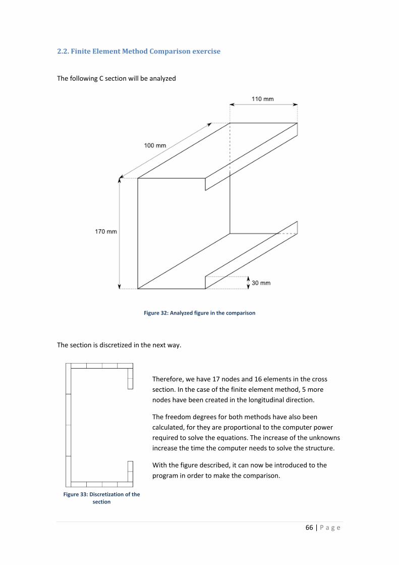
66 | P a g e
2.2. Finite Element Method Comparison exercise
The following C section will be analyzed
Figure 32: Analyzed figure in the comparison
The section is discretized in the next way.
Therefore, we have 17 nodes and 16 elements in the cross
section. In the case of the finite element method, 5 more
nodes have been created in the longitudinal direction.
The freedom degrees for both methods have also been
calculated, for they are proportional to the computer power
required to solve the equations. The increase of the unknowns
increase the time the computer needs to solve the structure.
With the figure described, it can now be introduced to the
program in order to make the comparison.
Figure 33: Discretization of the section
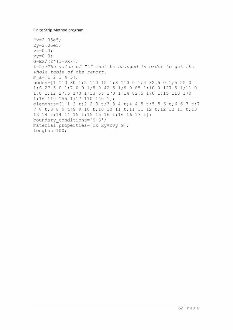
67 | P a g e
Finite Strip Method program:
Ex=2.05e5;
Ey=2.05e5;
vx=0.3;
vy=0.3;
G=Ex/(2*(1+vx));
t=5;%The value of “t” must be changed in order to get the
whole table of the report.
m_a=[1 2 3 4 5];
nodes=[1 110 30 1;2 110 15 1;3 110 0 1;4 82.5 0 1;5 55 0
1;6 27.5 0 1;7 0 0 1;8 0 42.5 1;9 0 85 1;10 0 127.5 1;11 0
170 1;12 27.5 170 1;13 55 170 1;14 82.5 170 1;15 110 170
1;16 110 155 1;17 110 140 1];
elements=[1 1 2 t;2 2 3 t;3 3 4 t;4 4 5 t;5 5 6 t;6 6 7 t;7
7 8 t;8 8 9 t;9 9 10 t;10 10 11 t;11 11 12 t;12 12 13 t;13
13 14 t;14 14 15 t;15 15 16 t;16 16 17 t];
boundary_conditions='S-S';
material_properties=[Ex Eyvxvy G];
lengths=100;