non linear classiﬁcation using kernel methods · non linear classiﬁcation using kernel methods...

Non Linear Classification using Kernel Methods

Aayush Mudgal12008

Sheallika Singh12665

Abstract

Linear Models are not rich enough to capture many of the real-world patterns andit is often desired to capture non-linear patterns in the data. We briefly look to-wards Support Vector Machines and Nearest Neighbors as Classification methods,that can be kernelized. We also look at different formulations of SVM’s, namelyC-SVM and nu-SVM. We depict the wide applicability and ease of Kernel SVMsthrough real-world problems like in face detection, handwritten character detec-tion, spam/non-spam classification.

1 Introduction

Kernel based methods have shown significant success in classification, regression as well as unsu-pervised learning problems. Kernel-based algorithms have shown to be successful in a wide areaof applications including in the context of object detection, gene expression, handwritten characterrecognition, spam mail detection, textual classification([5][4][9][7][6]. In Many of the classifica-tions problems, the classes may not be linearly separable. Clearly linear algorithms tend to givepoor results in these tasks.However Kernel Methods (wherever applicable), makes linear modelwork in non-linear settings. Such a mapping of data to a higher dimensions using kernel functions,helps to exhibit linear patterns in this higher dimension. It is also shown that different kernel meth-ods for classification can be reduced to optimization of a convex cost function. We primarily look attwo cases of Suport Vector Machines [3], namely C-SVM and Nu-SVM, and their Kernel counter-parts.We also look at other non-linear classifier K-nearest neighbors and its kernelised version.

2 Main Body

2.1 Non-Linear Algorithms in Kernel Feature Spaces

In most of the practical cases the Learning Set(L) is not linearly separable in the input space. Ker-nel functions essentially help to map the input space φ : X → F by a non-linear mapping φ toanother feature space F . F is usually of much higher dimension than the input space. Such higherdimensional representation of the input vectors, may result in vectors being linearly separated in themapped feature space. The idea is thus to learn develop the classifier in this feature space.

Kernel Trick: Any Learning algorithm that works entirely with inner products can be kernel-ized. A valid Kernel mapping 1, allows to work in the Feature space without explicitly requiringto calculate the vector representation in the Feature space (F). The easy computation of the kernelfunction (as it is in terms of inner products), helps to keep the computational complexity of thealgorithm in check and most often kernelization comes at a very little overhead. Kernel trick thusallows us to get the effect of working in F through a non-linear mapping where it might be possibleto develop linear algorithms. Since a kernel function is quite similar to just an inner product, it canbe visualized as a similarity metric. Such a visualization is quite common specially in the case of

1k: XxX → R is a valid kernel iff ∀x, y ∈ X , k(x, y) = 〈φ(x), φ(y)〉, where φ : X → F , where F is avalid inner product space

1

structured data (textual data, graphical data). Still the major tasks that remains is while choosing theright type of the algorithm. Radial Basis Function (rbf) 2, Polynomial3, Linear are some of the mostcommon types of kernels.

2.2 SVM Formulation (Separable Case)

Given an instance of Learning Set L given by {(xi, yi)|i = 1..n, xi ∈ X , yi ∈ {−1, 1}}, thesupport vector machines (SVM)[3] tries to maximize the margin.Separating hyperplane is in themidway between the margin planes. Maximising the margin we get convex optimization problemfor which the dual problem is as follows:

minα

1

2

n∑i=1

n∑j=1

αiαjyiyj〈xi, xj〉 −n∑i=1

αi

s.t.αi ≥ 1,∀i ∈ {1..n}n∑i=1

αiyi = 0

From Strong duality, the primal and dual problems have the same solution. Thus solving the dualproblem (a convex optimization problem) gives us the optimal solution α∗. The separating hyper-plane can be recalculated as follows: w∗ =

∑ni=1 αi

∗yi ∗xi. Complementary slackness condition isused to find the optimal w∗

0 , which is given by w∗0 = yj −

∑ni=1 α

∗i y

∗i 〈xi, xj〉, for some j satisfying

α∗i > 0

2.3 C-SVM Formulation (Non-Separable Case)

As observed in Section (??), the Normal SVM algorithm makes a very strong assumption that thelearning set is linearly separable. However such an assumption normally does not hold in practicalpurposes. Therefore C-SVM a modification of the normal SVM is more popularly used. As itrelaxes the condition that yig(xi) ≥ 1,∀i ∈ {1..n}. With the introduction of slack variables theconstraint is modified as, yig(xi) ≥ 1 − ξi,∀i ∈ {1..n}andξi ≥ 0. Such a modification allowsto give some penalties for mis-classification. The regular correctly classified vectors that are on themargin and beyond are represented by yig(xi) ≥ 1 and ξi = 0. Points that are correctly classifiedbut between the margin are represented by 0 < yig(xi) < 1, and 0 < ξi < 1, while the misclassifiedpoints are represented by yig(xi) < 0 and ξi > 1 The C-SVM requires the solution of the followingconvex optimization problem given by Equation (2.3). C is a regularization parameter (which istuned through cross-validation). Regularization parameter acts as a balance between widening themargin and allowing misclassified and margin points. A small C favors a larger margin. C=0, isequivalent to the normal svm problem.

minw,w0,ξ

||w||2

2+ C

n∑i=1

ξi

s.t.yig(xi) ≥ 1− ξi,∀i ∈ {1..n}(xi, yi) ∈ Lξi ≥ ∀i ∈ {1..n}(xi, yi) ∈ L

2K(x, x′) = exp

(− γ||x− x

′||2

)is a general case rbf kernel

3K(x, x′) = (xTx

′+ c)d is a general case polynomial kernel of degree d

2

The dual problem of Equation (2.3) is given as follows:

minα

1

2

n∑i=1

n∑j=1

αiαjyiyj〈xi, xj〉 −n∑i=1

αi

s.t.0 ≤ αi ≤ C,∀i ∈ {1..n}n∑i=1

αiyi = 0

From strong duality the solution to the dual problem gives the solution to the primal problem. Hencethe separating hyper-plane can be calculated from the solution of the dual problem as follows.

w∗ =

n∑i=1

αi∗yi ∗ xi

From the application of KKT conditions it follows that

w∗0 = yj −

n∑i=1

α∗i y

∗i 〈xi, xj〉

forsomej, s.t.0 ≤ αj ≤ 1

2.4 Nu-SVM Formulation

ν-SVC([2],[8]) is a variant of the soft margin problem of finding the optimal hyperplane [8]. Hereparameter C is replaced by a parameter ν ∈ [0, 1] which is the lower and upper bound on the numberof examples that are support vectors and that lie on the wrong side of the hyperplane, respectively.In case of C-SVM, C could have taken any real positive value, as opposed to the additional boundhere. We get a quadratic optimization problem as a dual problem which can be kernelised in thesimilar manner as C-SVC (shown later in section 2.4.1Proposition:(Connection between C-SVC and ν-SVC[1][8])If ν-SVC leads to ρ ≥ 0, then C-SVC, with C set a priori to 1/mρ, leads to the same decision function. Despite the bound on thenumber of support vectors, ν SVM is difficult to optimize and thus not very suitable for big datasets.

2.4.1 Kernelization of SVM and C-SVM and ν-SVM

Both SVM and C-SVM can be solved by solving the corresponding dual problems. The dual prob-lem is almost similar to that of the Normal SVM problem, except that αi is bounded above by theregularization parameter. Input feature vectors, i.e. x ∈ X occur in the dual optimization problemin the form of inner products. Hence the dual optimization problem can be kernalized in case ofboth SVM and C-SVM. The inner product 〈xi, xj〉 would be replaced by 〈φ(xi), φ(xj)〉, if the inputspace is mapped to a RKHS feature space F , where the mapping is satisfied by some kernel functionK. The Kernel Trick allows us to simplify the inner product 〈φ(xi), φ(xj)〉 by K(xi, xk. Howeverthe algorithm can be kernelized only if the input vectors appear in the form of inner products alsoduring the prediction step. In both the formulations any test vector x is given a label by:

sgn(w∗x+ w0)

=⇒ sgn(

n∑i=1

α∗i yi〈φ(xi), φ(x)〉

=⇒ sgn(

n∑i=1

α∗i yi〈K(xi, x)

Hence both the optimization problem and the decision function can be written in terms of only innerproduct of input space vectors, both SVM and C-SVM can be kernelized

3 Kernel Nearest neighbor[10]

In the k-nearest neighbor a query point is classified by finding the k closest neighbors (w.r.t. distancebetween the and query point) and then assigning the majority label among these k points to the

3

query point. The norm distance, which is used in k-nearest neighbor algorithm, can be denoted as:d(x, y) = ||x− y||The square of norm distance can be written as: d2(x, y) = 〈x, x〉 − 2× 〈x, y〉+ 〈y, y〉This square of norm distance can be written in form of inner product and thus we can use ’KernelTrick’ to kernelise k-nearest neighbor algorithm.

4 Simulation/Results

4.0.1 Spam-Non Spam Dataset

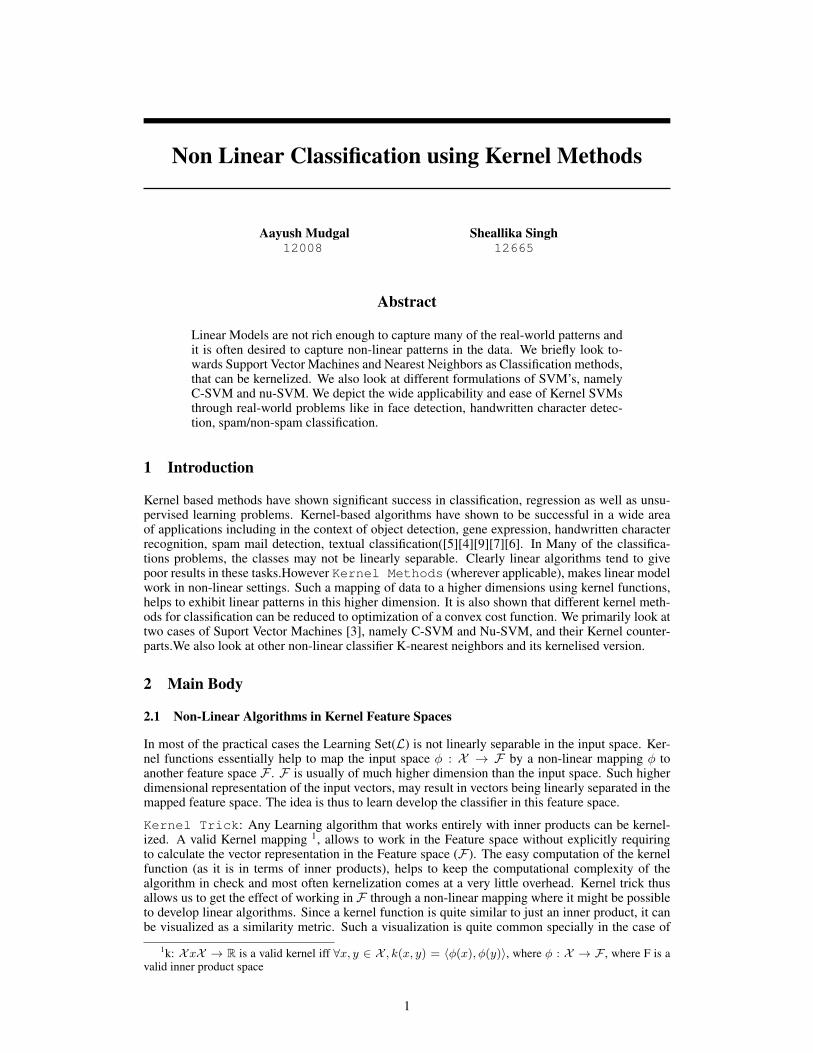
This is a 2-class dataset consisting of about 2800 e-mail messages with text,and subject. Each ofwhich is classified into spam (480) or non-spam messages. The 2-D visualization plots for differentKernel functions variations over the basic C-SVM classifiers along with the respective accuraciesare depicted in Figure(1).

Figure 1: Different Kernel Functions for C-SVM

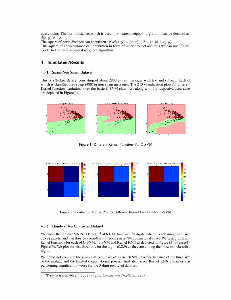
Figure 2: Confusion Matrix Plot for different Kernel Function for C-SVM

4.0.2 Handwritten Character Dataset

We chose the famous MNIST Data-set 4 of 60,000 handwritten digits, wherein each image is of size28x28 pixels, and can thus be considered as points in a 784 dimensional space We tested differentkernel functions for each of C-SVM, nu-SVM and Kernel KNN as depicted in Figure (3), Figure(4),Figure(5). We plot the visualizations for the digits (0,8,9) as they are among the most mis-classifieddigits.

We could not compute the gram matrix in case of Kernel KNN classifier, because of the huge sizeof the matrix, and the limited computational power. And also, since Kernel KNN classifier wasperforming significantly worse for the 3-digit restricted data-set.

4Data-set is available at http://yann.lecun.com/exdb/mnist/

4

http://yann.lecun.com/exdb/mnist/

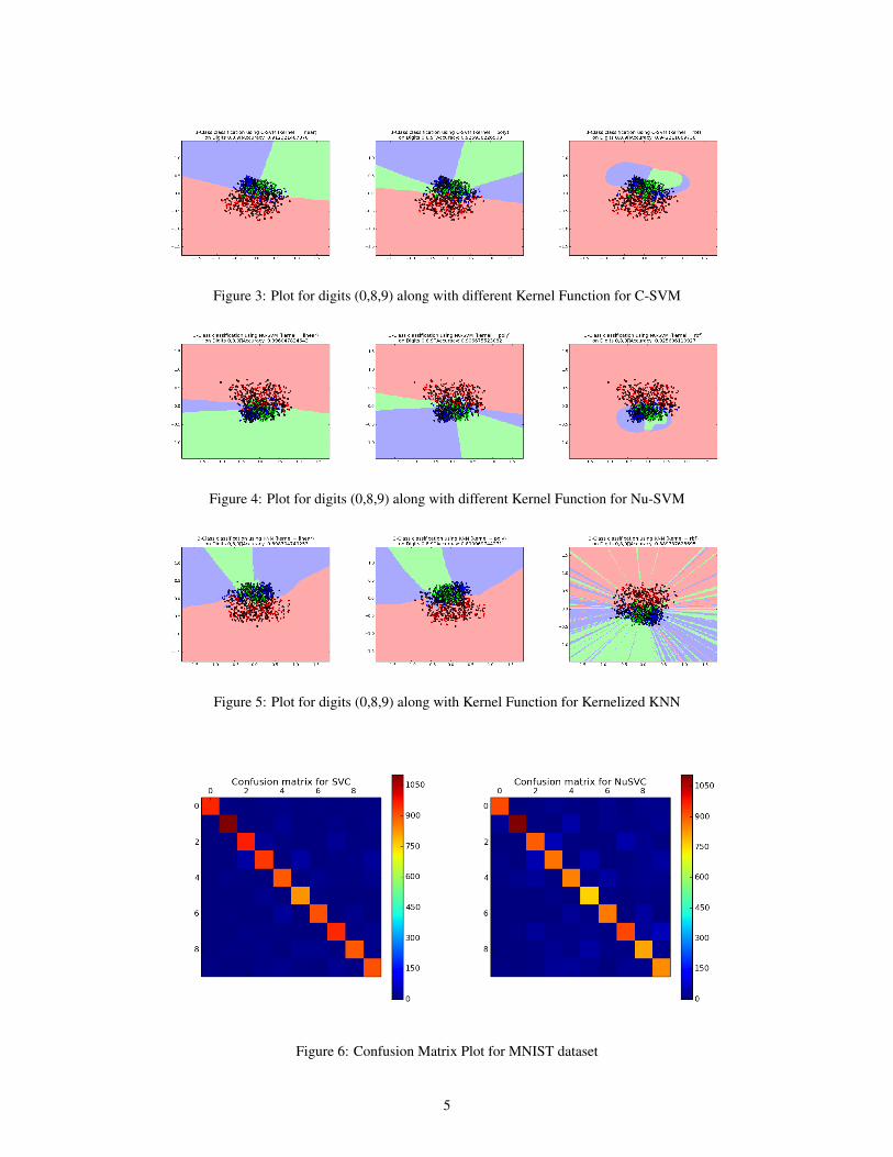
Figure 3: Plot for digits (0,8,9) along with different Kernel Function for C-SVM

Figure 4: Plot for digits (0,8,9) along with different Kernel Function for Nu-SVM

Figure 5: Plot for digits (0,8,9) along with Kernel Function for Kernelized KNN

Figure 6: Confusion Matrix Plot for MNIST dataset

5

4.0.3 Face Detection Data-set

We use the ATT FaceDatabase 5 and the FaceRec library 6 for face detection task. We used Fish-erFaces as a Feature Extractor, followed by our choice algorithms. We obtained the best validationaccuracy of 97.75% for the KNN with RBF kernel and number of nearest neighbor equals to 4.FisherFaces acts as a dimensional reduction techniques, making KNN scalable for larger data

5 Conclusions

In the case of the two class classification problem of spam and non-spam messages, we observerthat linear classifiers clearly outperform the other Kernel classifiers. Thus implying that there waslinearity in the input space. In such a situation, usage of kernel functions does not seem to addbenefit.

However in the case of MNIST data-set where the input space was observed to be non-linear, weobserve that the Kernelized Classifiers, almost always reported a higher accuracy. KNN Classifierwith a euclidean metric was the worst classifier for this task. This primarily can be related to the waythat different digits can be written in different styles, which have different distances among them.

We also noted that Kernel Nearest Neighbor Classifier suffered from longer training times, and alsoincreased requirement of computations during the testing time. Kernel functions compensated forthe increase in the training time, through significant increases in accuracy in some cases. We observethat C-SVM emerges as the choice classifier to be used in practice.

The success of a kernel classifier thus deeply dependent on the chosen kernel function. Any failureof Kernel method is probably because of the incapability in selecting the desired kernel function thatcould model such complex data. Construction of a proper kernel remains an important obstacle forthe successful application of these algorithms in some cases.

References[1] D. Burges and C. Crisp. A geometric interpretation of v- svm classifiers. Advances in neural

information processing systems, 12(12):244, 2000.[2] P.-H. Chen, C.-J. Lin, and B. Scholkopf. A tutorial on ν-support vector machines. Applied

Stochastic Models in Business and Industry, 21(2):111–136, 2005.[3] C. Cortes and V. Vapnik. Support-vector networks. Machine learning, 20(3):273–297, 1995.[4] D. Decoste and B. Scholkopf. Training invariant support vector machines. Machine learning,

46(1-3):161–190, 2002.[5] Y. LeCun, L. Jackel, L. Bottou, C. Cortes, J. S. Denker, H. Drucker, I. Guyon, U. Muller,

E. Sackinger, P. Simard, et al. Learning algorithms for classification: A comparison on hand-written digit recognition. Neural networks: the statistical mechanics perspective, 261:276,1995.

[6] K.-R. Muller, S. Mika, G. Ratsch, K. Tsuda, and B. Scholkopf. An introduction to kernel-basedlearning algorithms. Neural Networks, IEEE Transactions on, 12(2):181–201, 2001.

[7] D. Roobaert and M. M. Van Hulle. View-based 3d object recognition with support vectormachines. In Neural Networks for Signal Processing IX, 1999. Proceedings of the 1999 IEEESignal Processing Society Workshop., pages 77–84. IEEE, 1999.

[8] B. Scholkopf, A. J. Smola, R. C. Williamson, and P. L. Bartlett. New support vector algorithms.Neural computation, 12(5):1207–1245, 2000.

[9] S. P. Scholkopf, V. Vapnik, and A. Smola. Improving the accuracy and speed of support vectormachines. Advances in neural information processing systems, 9:375–381, 1997.

[10] K. Yu, L. Ji, and X. Zhang. Kernel nearest neighbor algorithm. Neural Processing Letters,15(2):147–156, 2002.

5Dataset is available at http://www.cl.cam.ac.uk/research/dtg/attarchive/facedatabase.html

6FaceRec library is available for Python at https://github.com/bytefish/facerec

6

http://www.cl.cam.ac.uk/research/dtg/attarchive/facedatabase.html

http://www.cl.cam.ac.uk/research/dtg/attarchive/facedatabase.html

https://github.com/bytefish/facerec

# Part of code used for development# sklearn does not provide an interface for Kernel KNN Classifier, the

same was thus implemented by seeking help fromhttps://github.com/jsantarc/Kernel-Nearest-Neighbor-Algorithm-in-Python-

# visualization code for MNIST data-setimport os, structfrom array import array as pyarrayfrom numpy import arange, array, int8, uint8, zeros, array, appendfrom struct import unpackfrom skimage.feature import hogfrom sklearn.cross_validation import StratifiedShuffleSplitimport cv2import matplotlib.pyplot as pltfrom sklearn.grid_search import GridSearchCVfrom sklearn.decomposition import PCAfrom time import timefrom operator import itemgetterfrom scipy.stats import randintimport cv2import numpy as npfrom sklearn import svm, ensemble , treefrom sklearn.metrics import confusion_matriximport pylab as plfrom cPickle import dump, loadfrom skimage.feature import hogimport skimagefrom matplotlib.colors import ListedColormapfrom sklearn.utils import shuffleimport numpy as npfrom sklearn import neighbors, datasetsfrom sklearn.metrics.pairwise import pairwise_kernelsimport numpy as npFILTER="hog"def load_mnist(dataset="training", digits=np.arange(10), path="."):

"""Loads MNIST files into 3D numpy arrays

Adapted from: http://abel.ee.ucla.edu/cvxopt/_downloads/mnist.pyand http://g.sweyla.com/blog/2012/mnist-numpy/"""

if dataset == "training":fname_img = os.path.join(path, ’train-images.idx3-ubyte’)fname_lbl = os.path.join(path, ’train-labels.idx1-ubyte’)

elif dataset == "testing":fname_img = os.path.join(path, ’t10k-images.idx3-ubyte’)fname_lbl = os.path.join(path, ’t10k-labels.idx1-ubyte’)

else:raise ValueError("dataset must be ’testing’ or ’training’")

flbl = open(fname_lbl, ’rb’)magic_nr, size = struct.unpack(">II", flbl.read(8))lbl = pyarray("b", flbl.read())flbl.close()

fimg = open(fname_img, ’rb’)magic_nr, size, rows, cols = struct.unpack(">IIII", fimg.read(16))img = pyarray("B", fimg.read())fimg.close()

ind = [ k for k in range(size) if lbl[k] in digits ]N = len(ind)

7

images = zeros((N, rows, cols), dtype=uint8)labels = zeros((N, 1), dtype=int8)for i in range(len(ind)):

images[i] = array(img[ ind[i]*rows*cols : (ind[i]+1)*rows*cols]).reshape((rows, cols))

labels[i] = lbl[ind[i]]

return images, labelsdef extract_hog(X_train_name,Y_name, save=True, filetype="Train"):

hogs = []count =0total = len(Y_name)for imgfile in X_train_name:

cv2.imwrite("temp.png", imgfile)img = cv2.imread("temp.png")#print imgimg = cv2.resize(img,(28,28))gray_img = cv2.cvtColor(img, cv2.COLOR_BGR2GRAY)fd = hog(gray_img,normalise =True, orientations=9,

pixels_per_cell=(14, 14), cells_per_block=(1,1),visualise=False)

# comp = skimage.feature.hog(img)hogs.append( fd )# lens.add(comp.shape)#print type(comp)count+=1print "done", count, total

X_train = np.array(hogs , ’float64’ )

if save==True:dump( X_train, open( FILTER+filetype+"1", "wb" ) )dump(Y_name, open("Y_"+filetype+"1", "wb"))print "Files stored: "+FILTER+filetype +"and Y_"+filetype

return X_train, np.array(Y_name)

def refineSets(images, labels, size):result = zeros(10)count =0X=[]Y=[]

for i in range(0,len(labels)):label = labels[i]feature = images[i]if result[label]<=size:

X.append(feature)Y.append(label)count+=1result[label]+=1

if count > size*10:break

return array(X), np.array(Y)

def saveFeatures(X_name, Y_name, save=True,filetype="Train"):

if FILTER=="hog":return extract_hog(X_name,Y_name,save, filetype)

# help sought fromhttps://github.com/jsantarc/Kernel-Nearest-Neighbor-Algorithm-in-Python-

def KernelKNNClassifierFit(X,Y,Kernel,Parameters):Y= np.array(Y)

8

#Number of training samplesN=len(X);#Array sorting value of kernels k(x,x)Gram_Matrix=np.zeros(N);#Calculate Kernel vector between same vectors Kxx[n]=k(X[n,:],X[n,:])#dummy for kernel namefor n in range(0,N):

Gram_Matrix[n]=pairwise_kernels(X[n],metric=Kernel,filter_params=Parameters)

return Gram_Matrix

def predict(X_test,X_train,Kernel,Parameters, Gram_Matrix, Y_train,n_neighbors=1):

Nz=len(X_test)#Empty list of predictionsyhat= np.zeros(Nz);#number of samples for classification#Number of training samplesNx=len(X_train);#Dummy variable Vector of ones used to get rid of one loop for k(z,z)Ones=np.ones(Nx);

#squared Euclidean distance in kernel space for each training sampleDistance=np.zeros(Nx)# Index of sorted valuesIndex= np.zeros(Nx)

# calculate pairwise kernels beteen Training samples and predictionsamples

Kxz=pairwise_kernels(X_train,X_test,metric=Kernel,filter_params=Parameters)

NaborsNumberAdress=range(0,n_neighbors)

#Calculate Kernel vector between same vectors Kxx[n]=k(Z[n,:],Z[n,:])

for n in range(0,Nz):# calculate squared Euclidean distance in kernel space for each

training sample#for one prediction#for m in range(0,Nx)#Distance[m]=|phi(x[m])-phi(z[n])|ˆ2=k(x,x)+k(z,z)-2k(z,x)

Distance =Gram_Matrix+pairwise_kernels(X_test[n],metric=Kernel,filter_params=Parameters)*Ones-2*Kxz[:,n]

#Distance indexes sorted from smallest to largestIndex=np.argsort(Distance.flatten());Index=Index.astype(int)

#get the labels of the nearest feature vectorsyl=list(Y_train[Index[NaborsNumberAdress]])#perform majority voteyhat[n]=max(set(yl), key=yl.count)

return(yhat)

if __name__ == "__main__":

# train_images, train_labels = refineSets(train_images, train_labels,1111) # working with smaller subset

# test_images, test_labels = refineSets(test_images, test_labels,111) # working with a smaller subset

9

retrain = raw_input("Feature Extraction??")

if retrain=="y":train_images,train_labels = load_mnist(’training’, digits=[8,9])test_images,test_labels = load_mnist(’testing’,digits=[8,9])X_train, Y_train = saveFeatures(train_images,train_labels)X_test, Y_test= saveFeatures(test_images, test_labels,save=True,

filetype="Test")Y_train=Y_train.flatten()Y_test = Y_test.flatten()

else:with open(FILTER+"Train1", ’rb’) as fp:

X_train = load(fp)with open("Y_Train1", ’rb’) as fp:

Y_train = load(fp)with open(FILTER+"Test1", ’rb’) as fp:

X_test = load(fp)with open("Y_Test1", ’rb’) as fp:

Y_test = load(fp)Y_train=Y_train.flatten()Y_test = Y_test.flatten()

# hog features extracted# i have the hog features, I need to apply SVM the kernel svm and

other stuff... and nearest neighbor classifier too,# i need to do some visualizations.. Need to add confusion matrix# Visualization help sought from

https://github.com/saradhix/mnist_svm/blob/master/plot_mnist_svm.pynum_samples_to_plot = 1000X_train, Y_train = shuffle(X_train, Y_train)X_train, Y_train = X_train[:num_samples_to_plot],

Y_train[:num_samples_to_plot]pca = PCA(n_components=2)X = pca.fit_transform(X_train)

print X.shapey=Y_train

h = .02 # step size in the meshn_neighbors=4# Create color mapscmap_light = ListedColormap([’#FFAAAA’, ’#AAFFAA’, ’#AAAAFF’])cmap_bold = ListedColormap([’#FF0000’, ’#00FF00’, ’#0000FF’])

for k in [’poly’]:# we create an instance of Neighbours Classifier and fit the data.if k==’linear’:

clf = KernelKNNClassifierFit(X,y,’linear’,0)clf1 = KernelKNNClassifierFit(X_train,Y_train,’linear’,0)Z1 = predict(X_test,

X_train,’linear’,0,clf1,Y_train,n_neighbors)accuracy = np.mean(Z1==Y_test)print accuracyraw_input()

elif k==’poly’:clf= KernelKNNClassifierFit(X,y,’poly’,3)clf1 = KernelKNNClassifierFit(X_train,Y_train,’poly’,3)Z1 = predict(X_test, X_train,’poly’,3,clf1,Y_train,n_neighbors)accuracy = np.mean(Z1==Y_test)print accuracy

elif k==’rbf’:clf= KernelKNNClassifierFit(X,y,’rbf’,1)clf1 = KernelKNNClassifierFit(X_train,Y_train,’rbf’,1)Z1 = predict(X_test, X_train,’rbf’,1,clf1,Y_train,n_neighbors)

10

accuracy = np.mean(Z1==Y_test)print accuracy

# I have gramMatrix in clf

# Plot the decision boundary. For that, we will assign a color toeach

# point in the mesh [x_min, m_max]x[y_min, y_max].x_min, x_max = X[:, 0].min() - 1, X[:, 0].max() + 1y_min, y_max = X[:, 1].min() - 1, X[:, 1].max() + 1xx, yy = np.meshgrid(np.arange(x_min, x_max, h),

np.arange(y_min, y_max, h))if k==’linear’:

Z=predict(np.c_[xx.ravel(), yy.ravel()], X,’linear’,0,clf,y,n_neighbors)

if k==’poly’:Z=predict(np.c_[xx.ravel(), yy.ravel()],

X,’poly’,3,clf,y,n_neighbors)if k==’rbf’:

Z=predict(np.c_[xx.ravel(), yy.ravel()],X,’cosine’,1,clf,y,n_neighbors)

print Z# Put the result into a color plotZ = Z.reshape(xx.shape)plt.figure()plt.pcolormesh(xx, yy, Z, cmap=cmap_light)

# Plot also the training pointsplt.scatter(X[:, 0], X[:, 1], c=y, cmap=cmap_bold)plt.xlim(xx.min(), xx.max())plt.ylim(yy.min(), yy.max())

plt.title("3-Class classification using KNN (kernel = "+k+")\n"+"on Digits 0,8,9\tAccuracy: " +str(accuracy))

plt.savefig("KNN089-Final"+k+".png")

# code for SVC, nuSVC MNISTimport os, structfrom array import array as pyarrayfrom numpy import arange, array, int8, uint8, zeros, array, appendfrom struct import unpackfrom skimage.feature import hogfrom sklearn.tree import DecisionTreeClassifierfrom sklearn.cross_validation import StratifiedShuffleSplitimport cv2import matplotlib.pyplot as pltfrom sklearn.grid_search import GridSearchCVfrom sklearn.metrics import confusion_matrix

from time import timefrom operator import itemgetterfrom scipy.stats import randintimport cv2import numpy as npfrom sklearn import svm, ensemble , treefrom sklearn.metrics import confusion_matriximport pylab as plfrom cPickle import dump, loadfrom skimage.feature import hogimport skimagefrom sklearn.neighbors import KNeighborsClassifier

11

from matplotlib.colors import ListedColormapFILTER="hog"def load_mnist(dataset="training", digits=np.arange(10), path="."):


















if save==True:dump( X_train, open( FILTER+filetype, "wb" ) )dump(Y_name, open("Y_"+filetype, "wb"))print "Files stored: "+FILTER+filetype +"and Y_"+filetype

12






return array(X), np.array(Y)def showconfusionmatrix(cm,typeModel):

pl.matshow(cm)pl.title(’Confusion matrix for ’+typeModel)pl.colorbar()pl.show()

def report(grid_scores, n_top=3):"""Report top n_top parameters settings, default n_top=3.

Args----grid_scores -- output from grid or random searchn_top -- how many to report, of top models

Returns-------top_params -- [dict] top parameter settings found in

search"""top_scores = sorted(grid_scores,

key=itemgetter(1),reverse=True)[:n_top]

for i, score in enumerate(top_scores):print("Model with rank: {0}".format(i + 1))print(("Mean validation score: "

"{0:.3f} (std: {1:.3f})").format(score.mean_validation_score,np.std(score.cv_validation_scores)))

print("Parameters: {0}".format(score.parameters))print("")

return top_scores[0].parametersdef run_gridsearch(X, y, clf, param_grid, cv=5):

"""Run a grid search for best Decision Tree parameters.

Args----X -- featuresy -- targets (classes)cf -- scikit-learn Decision Treeparam_grid -- [dict] parameter settings to testcv -- fold of cross-validation, default 5

Returns-------

13

top_params -- [dict] from report()"""print "GridSearchCV starting"grid_search = GridSearchCV(clf,

param_grid=param_grid,cv=cv)

start = time()print "Fit starting"grid_search.fit(X, y)

print(("\nGridSearchCV took {:.2f} ""seconds for {:d} candidate ""parameter settings.").format(time() - start,

len(grid_search.grid_scores_)))

top_params = report(grid_search.grid_scores_, 3)return top_params



if __name__ == "__main__":




if retrain=="y":train_images,train_labels = load_mnist(’training’)test_images,test_labels = load_mnist(’testing’)X_train, Y_train = saveFeatures(train_images,train_labels)X_test, Y_test= saveFeatures(test_images, test_labels,save=True,


else:with open(FILTER+"Train", ’rb’) as fp:

X_train = load(fp)with open("Y_Train", ’rb’) as fp:

Y_train = load(fp)with open(FILTER+"Test", ’rb’) as fp:

X_test = load(fp)with open("Y_Test", ’rb’) as fp:


# hog features extracted

# i have the hog features, I need to apply SVM the kernel svm andother stuff... and nearest neighbor classifier too,

# i need to do some visualizations.. Need to add confusion matrix# C_range = np.logspace(-2,2,4)gamma_range=[2,4,6]param_grid = {

"kernel" :[’poly’,’rbf’, ’linear’],"gamma": gamma_range,’nu’ : [0.5]

}

14

clf = svm.NuSVC(kernel=’rbf’,gamma=6)clf.fit(X_train,Y_train)predicted = clf.predict(X_test)cm = confusion_matrix(predicted, Y_test)showconfusionmatrix(cm, "NuSVC")print "NuSVC accuracy" ,np.mean(Y_test==predicted)

clf = svm.SVC(kernel=’rbf’,gamma=6)clf.fit(X_train,Y_train)predicted = clf.predict(X_test)cm = confusion_matrix(predicted, Y_test)showconfusionmatrix(cm, ’SVC’)print "SVC accuracy" ,np.mean(Y_test==predicted)

# dump(ts_gs, open( "model1", "wb" ))

# GridSearchCV took 836.51 seconds for 24 candidate parameter settings.# Model with rank: 1# Mean validation score: 0.963 (std: 0.002)# Parameters: {’kernel’: ’rbf’, ’C’: 4.6415888336127775, ’gamma’: 2}

# Model with rank: 2# Mean validation score: 0.963 (std: 0.002)# Parameters: {’kernel’: ’rbf’, ’C’: 4.6415888336127775, ’gamma’: 4}

# Model with rank: 3# Mean validation score: 0.963 (std: 0.002)# Parameters: {’kernel’: ’rbf’, ’C’: 4.6415888336127775, ’gamma’: 6}

# print clf.score(hog_test_images,test_labels)

# i have the hog features, I need to apply SVM the kernel svm andother stuff... and nearest neighbor classifier too,

# i need to do some visualizations.. Need to add confusion matrix

# Nu-SVM parameters

# code for Kernel KNN MNISTimport os, structfrom array import array as pyarrayfrom numpy import arange, array, int8, uint8, zeros, array, appendfrom struct import unpackfrom skimage.feature import hogfrom sklearn.tree import DecisionTreeClassifierfrom sklearn.cross_validation import StratifiedShuffleSplitimport cv2import matplotlib.pyplot as pltfrom sklearn.grid_search import GridSearchCVfrom sklearn.decomposition import PCAfrom time import timefrom operator import itemgetterfrom scipy.stats import randintimport cv2import numpy as npfrom sklearn import svm, ensemble , treefrom sklearn.metrics import confusion_matriximport pylab as plfrom cPickle import dump, loadfrom skimage.feature import hog

15

import skimagefrom matplotlib.colors import ListedColormapfrom sklearn.utils import shuffleimport numpy as npfrom sklearn import neighbors, datasetsfrom sklearn.metrics.pairwise import pairwise_kernelsimport numpy as npFILTER="hog"def load_mnist(dataset="training", digits=np.arange(10), path="."):

















16


if save==True:dump( X_train, open( FILTER+filetype+"1", "wb" ) )dump(Y_name, open("Y_"+filetype+"1", "wb"))print "Files stored: "+FILTER+filetype +"and Y_"+filetype






return array(X), np.array(Y)




def KernelKNNClassifierFit(X,Y,Kernel,Parameters):Y= np.array(Y)#Number of training samplesN=len(X);#Array sorting value of kernels k(x,x)Gram_Matrix=np.zeros(N);#Calculate Kernel vector between same vectors Kxx[n]=k(X[n,:],X[n,:])#dummy for kernel namefor n in range(0,N):


return Gram_Matrix

def predict(X_test,X_train,Kernel,Parameters, Gram_Matrix, Y_train,n_neighbors=1):

Nz=len(X_test)#Empty list of predictionsyhat= np.zeros(Nz);#number of samples for classification#Number of training samplesNx=len(X_train);#Dummy variable Vector of ones used to get rid of one loop for k(z,z)Ones=np.ones(Nx);

#squared Euclidean distance in kernel space for each training sampleDistance=np.zeros(Nx)# Index of sorted valuesIndex= np.zeros(Nx)

17








#Distance indexes sorted from smallest to largestIndex=np.argsort(Distance.flatten());Index=Index.astype(int)


return(yhat)

if __name__ == "__main__":




if retrain=="y":train_images,train_labels = load_mnist(’training’ )test_images,test_labels = load_mnist(’testing’)X_train, Y_train = saveFeatures(train_images,train_labels)X_test, Y_test= saveFeatures(test_images, test_labels,save=True,


else:with open(FILTER+"Train", ’rb’) as fp:

X_train = load(fp)with open("Y_Train", ’rb’) as fp:

Y_train = load(fp)with open(FILTER+"Test", ’rb’) as fp:

X_test = load(fp)with open("Y_Test", ’rb’) as fp:


# hog features extracted# i have the hog features, I need to apply SVM the kernel svm and

other stuff... and nearest neighbor classifier too,# i need to do some visualizations.. Need to add confusion matrix# Visualization help sought from

https://github.com/saradhix/mnist_svm/blob/master/plot_mnist_svm.py

18

n_neighbors=4

for k in [’poly’, ’linear’,’rbf’]:# we create an instance of Neighbours Classifier and fit the data.if k==’linear’:

clf1 = KernelKNNClassifierFit(X_train,Y_train,’linear’,0)Z1 = predict(X_test,

X_train,’linear’,0,clf1,Y_train,n_neighbors)accuracy = np.mean(Z1==Y_test)print "linear",accuracy

elif k==’cosine’:clf1 = KernelKNNClassifierFit(X_train,Y_train,’cosine’,1)Z1 = predict(X_test,

X_train,’cosine’,1,clf1,Y_train,n_neighbors)accuracy = np.mean(Z1==Y_test)print "Cosine",accuracy

elif k==’rbf’:clf1 = KernelKNNClassifierFit(X_train,Y_train,’rbf’,2)Z1 = predict(X_test, X_train,’rbf’,2,clf1,Y_train,n_neighbors)accuracy = np.mean(Z1==Y_test)print "RBF",accuracy


# Cosine 0.94500723589# linear 0.945489628558# RBF 0.945489628558

# code for Kernel KNN classifier spam-non spamfrom os import listdirfrom os.path import isfile, joinimport sysimport numpyimport cPickle as pickleimport collections, reimport scipy.sparsefrom sklearn import svmfrom sklearn.feature_extraction.text import CountVectorizerfrom sklearn.feature_extraction.text import CountVectorizerfrom sklearn.naive_bayes import MultinomialNBfrom sklearn.lda import LDAfrom nltk.stem import PorterStemmer, WordNetLemmatizerfrom sklearn.linear_model import Perceptronfrom sklearn.feature_extraction.text import TfidfVectorizerimport cv2import numpy as npfrom sklearn import svm, ensemble , treefrom sklearn.metrics import confusion_matriximport pylab as plfrom cPickle import dump, loadfrom skimage.feature import hogimport skimagefrom matplotlib.colors import ListedColormapfrom sklearn.utils import shuffleimport numpy as npfrom sklearn import neighbors, datasetsfrom sklearn.metrics.pairwise import pairwise_kernelsimport numpy as npfrom sklearn.decomposition import PCA

def createCorpus(data,i, binaryX="False", stopWords=None,lemmatize="False", tfidf= "False", useidf="True"): # will vectorizeBOG using frequency as the parameter and will return the requiredarrays

19

X_train =[]X_test=[]Y_train=[]Y_test=[]

for key in data:if key in i:

for filename in data[key]:text = data[key][filename][0]if lemmatize == "True":

port = WordNetLemmatizer()text = " ".join([port.lemmatize(k,"v") for k in

text.split()])X_test.append(text)Y_test.append(data[key][filename][1])

else:for filename in data[key]:

text = data[key][filename][0]if lemmatize == "True":

port = WordNetLemmatizer()text = " ".join([port.lemmatize(k,"v") for k in

text.split()])X_train.append(text)Y_train.append(data[key][filename][1])

if tfidf == "False":vectorizer = CountVectorizer(min_df=1, binary= binaryX,

stop_words=stopWords)X_train_ans = vectorizer.fit_transform(X_train)X_test_ans = vectorizer.transform(X_test)return X_train_ans, Y_train, X_test_ans,Y_test

elif tfidf == "True":vectorizer = TfidfVectorizer(min_df=1, use_idf=useidf)X_train_ans = vectorizer.fit_transform(X_train)X_test_ans = vectorizer.transform(X_test)

return X_train_ans, Y_train, X_test_ans,Y_test


def KernelKNNClassifierFit(X,Y,Kernel,Parameters):Y= numpy.array(Y)#Number of training samplesN=len(X);#Array sorting value of kernels k(x,x)Gram_Matrix=numpy.zeros(N);#Calculate Kernel vector between same vectors Kxx[n]=k(X[n,:],X[n,:])#dummy for kernel namefor n in range(0,N):


return Gram_Matrix

def predict(X_test,X_train,Kernel,Parameters, Gram_Matrix, Y_train,n_neighbors=1):Y_train=np.array(Y_train)Nz=len(X_test)#Empty list of predictionsyhat= numpy.zeros(Nz);#number of samples for classification#Number of training samplesNx=len(X_train);#Dummy variable Vector of ones used to get rid of one loop for k(z,z)Ones=numpy.ones(Nx);

20

#squared Euclidean distance in kernel space for each training sampleDistance=numpy.zeros(Nx)# Index of sorted valuesIndex= numpy.zeros(Nx)








#Distance indexes sorted from smallest to largestIndex=numpy.argsort(Distance.flatten());Index=Index.astype(int)


return(yhat)

def crossValidation(data,Parameters):n_neighbors=4accuracy=0 # with frequencyfor i in [0]:

testSet = [2*i+1,2*i+2]X_train, Y_train,X_test,Y_test = createCorpus(data,testSet,

binaryX="False", stopWords="english", lemmatize="False") #with frequency

X_train= X_train.todense()X_test=X_test.todense()# print "Fitting"num_samples_to_plot = 1000X_train, Y_train = shuffle(X_train, Y_train)X_train, Y_train = X_train[:num_samples_to_plot],

Y_train[:num_samples_to_plot]pca = PCA(n_components=2)X = pca.fit_transform(X_train)

print X.shapey=Y_train

h = .02 # step size in the meshn_neighbors=4# Create color mapscmap_light = ListedColormap([’#FFAAAA’, ’#AAFFAA’, ’#AAAAFF’])cmap_bold = ListedColormap([’#FF0000’, ’#00FF00’, ’#0000FF’])

for k in [’cosine’, ’linear’, ’rbf’]:

21

# we create an instance of Neighbours Classifier and fit thedata.

if k==’linear’:clf = KernelKNNClassifierFit(X,y,’linear’,0)clf1 = KernelKNNClassifierFit(X_train,Y_train,’linear’,0)Z1 = predict(X_test,

X_train,’linear’,0,clf1,Y_train,n_neighbors)accuracy = np.mean(Z1==Y_test)print accuracy

elif k==’cosine’:clf= KernelKNNClassifierFit(X,y,’cosine’,1)clf1 = KernelKNNClassifierFit(X_train,Y_train,’cosine’,1)Z1 = predict(X_test,

X_train,’cosine’,1,clf1,Y_train,n_neighbors)accuracy = np.mean(Z1==Y_test)print accuracy

elif k==’cosine’:clf= KernelKNNClassifierFit(X,y,’rbf’,1)clf1 = KernelKNNClassifierFit(X_train,Y_train,’rbf’,1)Z1 = predict(X_test,

X_train,’rbf’,1,clf1,Y_train,n_neighbors)accuracy = np.mean(Z1==Y_test)print accuracy


# Plot the decision boundary. For that, we will assign a colorto each

# point in the mesh [x_min, m_max]x[y_min, y_max].x_min, x_max = X[:, 0].min() - 1, X[:, 0].max() + 1y_min, y_max = X[:, 1].min() - 1, X[:, 1].max() + 1xx, yy = np.meshgrid(np.arange(x_min, x_max, h),

np.arange(y_min, y_max, h))if k==’linear’:

Z=predict(np.c_[xx.ravel(), yy.ravel()], X,’linear’,0,clf,y,n_neighbors)

elif k==’cosine’:Z=predict(np.c_[xx.ravel(), yy.ravel()],

X,’cosine’,1,clf,y,n_neighbors)elif k==’rbf’:

Z=predict(np.c_[xx.ravel(), yy.ravel()],X,’rbf’,1,clf,y,n_neighbors)

print Z# Put the result into a color plotZ = Z.reshape(xx.shape)plt.figure()plt.pcolormesh(xx, yy, Z, cmap=cmap_light)

# Plot also the training pointsplt.scatter(X[:, 0], X[:, 1], c=y, cmap=cmap_bold)plt.xlim(xx.min(), xx.max())plt.ylim(yy.min(), yy.max())

plt.title("2-Class classification KernelKNN (kernel = "+k+")\nAccuracy="+str(accuracy))

plt.savefig("KNN-SPAM"+k+".png")

if __name__ == "__main__":loadedData=pickle.load( open( "loadedData", "rb" ) )# questions = ["3a","3b","3c", "2ab"]

22

# questions = ["1a"]#for q in questions:# print "---------------------------"for C in [1]:

crossValidation(loadedData,C)# print "--------------------------"

#RBF: Accuracy 0.886620992173 Gamma 0.1# Cosine Accuracy 0.888695925627 Gamma 1

# code for faceDetection, modified for use fromhttps://github.com/bytefish/facerec

import sys, ossys.path.append("../..")# import facerec modulesfrom facerec import *from facerec.feature import Fisherfaces, SpatialHistogram, Identityfrom facerec.distance import EuclideanDistance, ChiSquareDistancefrom facerec.classifier import NearestNeighborfrom facerec.classifier import SVM

from facerec.model import PredictableModelfrom facerec.validation import KFoldCrossValidationfrom facerec.visual import subplotfrom facerec.util import minmax_normalizefrom facerec.serialization import save_model, load_model# import numpy, matplotlib and loggingimport numpy as np# try to import the PIL Image moduletry:

from PIL import Imageexcept ImportError:

import Imageimport matplotlib.cm as cmimport loggingimport matplotlib.pyplot as pltimport matplotlib.cm as cmfrom facerec.lbp import LPQ, ExtendedLBPimport cv2from os.path import exists, isdir, basename, join, splitextfrom os import makedirs,systemfrom glob import globfrom random import sample, seedfrom scipy import ones, mod, arrayfrom sklearn import svm, ensemble , treefrom sklearn.metrics import confusion_matriximport pylab as plfrom cPickle import dump, loadfrom skimage.feature import hogimport skimageimport picklefrom sklearn.cross_validation import KFoldimport subprocess

numTrain=10numClasses=40trainDir = sys.argv[1]

def get_class(datasetpath, numClasses):classes_paths = [files

for files in glob(datasetpath.strip() + "/*")if isdir(files)]

23

classes_paths.sort()classes = [basename(class_path) for class_path in classes_paths]classes = classes[:numClasses]return classes

def imgfiles(path, extensions):all_files = []all_files.extend([join(path, basename(fname))

for fname in glob(path + "/*")if splitext(fname)[-1].lower() in extensions])

return all_files

def readImage(X_fileName):feats = []for imgfile in X_fileName:

im = Image.open(imgfile)im = im.convert("L")feats.append(np.asarray(im, dtype=np.uint8))

return featsdef all_images(numTotal, dir_path, classes):

all_images = []all_images_class_labels = []for i, imageclass in enumerate(classes):

path = join(dir_path, imageclass)extensions = [".pgm"]imgs = imgfiles(path, extensions)imgs = sample(imgs, numTotal)all_images = all_images + imgsclass_labels = list(i * ones(numTotal))all_images_class_labels = all_images_class_labels + class_labels

all_images_class_labels = array(all_images_class_labels, ’int’)all_images = readImage(all_images)return all_images, all_images_class_labels

if __name__ == "__main__":

classes = get_class(trainDir, numClasses)X , y = all_images(numTrain , trainDir, classes) # images are read

suitably

feature = Fisherfaces()# Define a 1-NN classifier with Euclidean Distance:# classifier = NearestNeighbor(dist_metric=EuclideanDistance(), k=1)classifier=NearestNeighbor(dist_metric=EuclideanDistance(), k=1)# Define the model as the combinationmy_model = PredictableModel(feature=feature, classifier=classifier)# Compute the Fisherfaces on the given data (in X) and labels (in y):my_model.compute(X, y)# We then save the model, which uses Pythons pickle module:dump( my_model, open( "model", "wb" ) )with open("model", ’rb’) as fp:

model= load(fp)

# Then turn the first (at most) 16 eigenvectors into grayscale# images (note: eigenvectors are stored by column!)E = []for i in xrange(min(model.feature.eigenvectors.shape[1], 16)):

e = model.feature.eigenvectors[:,i].reshape(X[0].shape)E.append(minmax_normalize(e,0,255, dtype=np.uint8))

# Plot them and store the plot to "python_fisherfaces_fisherfaces.pdf"subplot(title="Fisherfaces", images=E, rows=4, cols=4,

sptitle="Fisherface", colormap=cm.jet, filename="fisherfaces.png")# Perform a 10-fold cross validationcv = KFoldCrossValidation(model, k=10)cv.validate(X, y)

24

# And print the result:cv.print_results()

25

non linear classiﬁcation using kernel methods · non linear classiﬁcation using kernel methods...

Documents