Non-Euclidean Contraction Theoryfor Robust Nonlinear Stability

Alexander Davydov, Student Member, IEEE, Saber Jafarpour, Member, IEEE, and Francesco Bullo, Fellow, IEEE

Abstract—We study necessary and sufficient conditions forcontraction and incremental stability of dynamical systems withrespect to non-Euclidean norms. First, we introduce weak pair-ings as a framework to study contractivity with respect toarbitrary norms, and characterize their properties. We introduceand study the sign and max pairings for the `1 and `∞ norms,respectively. Using weak pairings, we establish five equivalentcharacterizations for contraction, including the one-sided Lips-chitz condition for the vector field as well as matrix measure andDemidovich conditions for the corresponding Jacobian. Third, weextend our contraction framework in two directions: we proveequivalences for contraction of continuous vector fields and weformalize the weaker notion of equilibrium contraction, whichensures exponential convergence to an equilibrium. Finally, asan application, we provide (i) incremental input-to-state stabilityand finite input-state gain properties for contracting systems,and (ii) a general theorem about the Lipschitz interconnection ofcontracting systems, whereby the Hurwitzness of a gain matriximplies the contractivity of the interconnected system.

I. INTRODUCTION

Problem description and motivation: A vector field is con-tracting if its flow map is a contraction or, equivalently, ifany two solutions approach one another exponentially fast.Contracting systems feature highly-ordered asymptotic behav-ior. First, initial conditions are forgotten. Second, a uniqueequilibrium is globally exponential stable when the vectorfield is time-invariant and two natural Lyapunov functions areautomatically available (i.e., the distance to the equilibriumand the norm of the vector field). Third, a unique periodicsolution is globally exponentially stable when the vector fieldis periodic; in other words, contracting system entrain toperiodic inputs. Fourth and last, contracting systems enjoy nat-ural robustness properties such as input-to-state stability andfinite input-state gain in the presence of (Lipschitz continuous)unmodeled dynamics. Because of these highly-ordered anddesirable behaviors, contracting systems are of great interestfor engineering problems.

Contraction theory aims to combine, in a unified coherentframework, results from Lyapunov stability theory, incremen-tal stability, fixed point theorems, monotone systems theory,and the geometry of Banach, Riemannian and Finsler spaces.Classical approaches primarily study contraction with respectto the `2 norm for continuously differentiable vector fields.

This work was supported in part by the Defense Threat Reduction Agencyunder Contract No. HDTRA1-19-1-0017.

Authors are with the Department of Mechanical Engineering and theCenter for Control, Dynamical Systems, and Computation, Universityof California, Santa Barbara, 93106-5070, USA. (davydov, saber,bullo@ucsb.edu)

However, recent works have shown that stability can be stud-ied more systematically and efficiently using non-Euclideannorms (e.g., `1, `∞ and polyhedral norms) for large classesof network systems, including biological transcriptional sys-tems [50], Hopfield neural networks [49], chemical reactionnetworks [1], traffic networks [14], [12], [13], multi-vehiclesystems [46], and coupled oscillators [51], [6]. Moreover, forlarge-scale systems, error analysis based on the `∞ norm maymore accurately capture the effect of bounded perturbations.As compared with the `2 norm, there is only limited work onnon-Euclidean contraction theory.

It is well known that contraction with respect to the `2 normis established via a test on the Jacobian of the vector field; it isalso true however that an integral (derivative-free) test on thevector field itself is equivalent. While some differential testsare available for non-Euclidean norms, much less is knownabout the corresponding integral tests. We note that computingJacobians for large-scale networks may be computationallyintensive and so derivative-free contraction tests are desirable.In this paper, we aim to characterize differential and integraltests for arbitrary norms, paying special attention to the `1 and`∞ norms, and provide a unifying framework for differentialand integral tests.

Literature review: Contraction mappings in dynamical sys-tems via matrix measures have been studied extensively andcan be traced back to Lewis [36], Demidovich [21] andKrasovskiı [35]. Matrix measures and numerical methods fordifferential equations have been studied by Dahlquist [16] andLozinskii [39] in as early as 1958; see also the influentialsurvey by Strom [54]. Finally, matrix measures were appliedto control problems by Desoer and Vidyasagar in [22], [23],[55] and contraction theory was first introduced by Lohmillerand Slotine in [37]. Since then, numerous generalizationsto contraction theory have been proposed including partialcontraction [56], contraction on Riemannian and Finsler mani-folds, [52], [27], contraction for PDEs [3], transverse contrac-tion [43], contraction after short transients [45], and weak andsemi-contraction [33].

While the work of Lohmiller and Slotine explored differen-tial conditions for contraction for the `2 norm, related integralconditions have been studied in the literature under suchvarious names as the one-sided Lipschitz condition in [30],the QUAD condition in [40], the nonlinear measure [49], thedissipative Lipschitz condition [10], and incremental quadraticstability in [17]. A related unifying concept is the logarithmicLipschitz constant, advocated in [53], [4]. Moreover, the keyidea appears as early as [11], whereby minus the vector field iscalled uniformly increasing and in the work on discontinuous

arX

iv:2

103.

1226

3v3

[m

ath.

OC

] 2

5 Ju

l 202

1

Measure-bounded Demidovich One-sided LipschitzJacobian condition condition

µ2,P 1/2(Df(x)) ≤ b PDf(x) +Df(x)>P 2bP (x− y)>P(f(x)− f(y)

)≤ b‖x− y‖2P 1/2

µp,R(Df(x)) ≤ b (Rv |Rv|p−2)>RDf(x)v ≤ b‖v‖pp,R ((R(x− y)) |R(x− y)|p−2)>R(f(x)− f(y)) ≤ b‖x− y‖pp,R

µ1,R(Df(x)) ≤ b sign(Rv)>RDf(x)v ≤ b‖v‖1,R sign(Rx−Ry)>R(f(x)− f(y)) ≤ b‖x− y‖1,R

µ∞,R(Df(x)) ≤ b maxi∈I∞(Rv)

(RDf(x)v)i (Rv)i ≤ b‖v‖2∞,R maxi∈I∞(Rx−Ry)

(R (f(x)− f(y)))i((Rx)i − (Ry)i) ≤ b‖x− y‖2∞,R

TABLE ITABLE OF CONTRACTION EQUIVALENCES, THAT IS, EQUIVALENCES BETWEEN MEASURE BOUNDED JACOBIANS, DEMIDOVICH AND ONE-SIDED

LIPSCHITZ CONDITIONS. f : Rn → Rn IS A CONTINUOUSLY DIFFERENTIABLE VECTOR FIELD WITH JACOBIAN Df . EACH ROW CONTAINS THREEEQUIVALENT STATEMENTS, TO BE UNDERSTOOD FOR ALL x, y ∈ Rn AND ALL v ∈ Rn . THE FUNCTION sign : Rn → −1, 0, 1n IS THE ENTRYWISE

sign FUNCTION, IS THE ENTRYWISE PRODUCT, THE ABSOLUTE VALUE AND POWER OF A VECTOR ARE APPLIED ENTRYWISE. WE ADOPT THESHORTHAND I∞(v) = i ∈ 1, . . . , n | |vi| = ‖v‖∞. THE MATRIX P IS POSITIVE DEFINITE AND THE MATRIX R IS INVERTIBLE.

differential equations, see [26, Chapter 1, page 5] and refer-ences therein. Comparisons between the Lipschitz conditions,the QUAD condition, and contraction are detailed in [20], seealso [30, Section 1.10, Exercise 6].

Tests for contraction with respect to non-Euclidean non-differentiable norms have not been widely studied. Earlyresults on compartmental systems include [42, Theorem 2]and [32, Appendix 4]. The `1 integral test is used to studyneural networks in [49] and traffic networks in [12]. Recentwork [13] establishes that the `1 and `∞ norms are well suitedto study contraction of monotone systems. A comprehensiveunderstanding of connections between differential and integralconditions for these norms is desirable.

Aminzare and Sontag first drew connections between con-traction theory and so-called “semi-inner products” in [4],where they give conditions for contraction in Lp spaces. Sincethen, they have explored contraction with respect to arbitrarynorms in [6], [5], and [2], where arbitrary norms are usedto study synchronization of diffusively coupled systems andcontractivity of reaction diffusion PDEs. Most notably, in [5,Proposition 3] necessary and sufficient conditions for contrac-tion are given using Deimling pairings (see [25, Chapter 3] formore details on Deimling pairings). This paper builds uponthese underappreciated works and underutilized connections.

Contributions: Our first contribution is the definition ofweak pairings as a generalization of the classic Lumer pair-ings, as introduced in [41], [29]. We study various propertiesof weak pairings, including a useful curve norm derivative for-mula applicable to dynamical systems analysis. Additionally,we establish a key relationship between weak pairings andmatrix measures, generalizing a result by Lumer in [41]; werefer to this relationship as Lumer’s equality. For `p norms,p ∈ 1,∞, we present and characterize novel convenientchoices for weak pairings: the sign pairing for the `1 normand the max pairing for the `∞ norm. We argue that, due totheir connection with matrix measures, weak pairings are abroadly-applicable tool for contraction analysis.

Our second contribution is proving five equivalent charac-terizations of contraction for continuously differentiable vectorfields on Rn with respect to arbitrary norms. Using the

language of weak pairings, we prove the equivalence betweendifferential and integral tests for contraction; this result gener-alizes the known `2 norm results to non-differentiable normssuch as the `1 and `∞ norms. We show that three of thefive equivalences capture the matrix measure condition, thedifferential condition on the vector field (referred to as theDemidovich condition), and the integral condition (referred toas the one-sided Lipschitz condition). These results general-ize [5, Proposition 3] in the sense that (i) we draw an additionalconnection between the matrix measure of the Jacobian andthe weak pairing and (ii) use this connection and our signand max pairings to write the explicit differential and integralconditions in Table I.

Our third contribution is the extension of contraction theoryto vector fields that are only continuous. This extensiondemonstrates that contraction can be understood as a propertyof the vector field, independent of its Jacobian. In other words,this extension establishes the importance of weak pairings overclassical contraction approaches based on the Jacobian of thevector field and the stability of the linearized system.

Our fourth contribution is the formalization of equilibriumcontraction, a weaker form of contraction where all trajectoriesexponentially converge to an equilibrium. This notion has beenexplored for example, in [55, Chapter 2, Theorem 22] and [56,Theorem 1]. These approaches establish global exponentialconvergence under two conditions: the vector field can befactorized as f(t, x) = A(t, x)x and the matrix measure ofA(t, x) is uniformly negative. Our treatment of equilibriumcontraction demonstrates that these two conditions are onlysufficient, whereas we provide a necessary and sufficientcharacterization based upon the one-sided Lipschitz condition.

Our fifth contribution is proving novel robustness propertiesof contracting and equilibrium contracting vector fields. Forstrongly contracting systems we prove incremental input-to-state stability and provide novel input-state gain estimates.These results generalize [22, Theorem A] and [31, Theorem 1],where vector fields are required to have a special control-affinestructure. We additionally prove a novel result for contractionunder perturbations and are able to upper bound how far theunique equilibrium shifts.

Our sixth and final contribution is a general theorem aboutthe contractivity of the interconnection of contracting systems.Motivated by applications to large scale systems, we providea sufficient condition for contraction and establish optimalcontraction rates for interconnected systems. This theorem isthe counterpart for contracting system of the classic theoremabout the interconnection of dissipative systems, e.g., see [8,Chapter 2]. This treatment generalizes the results in [54,Section 5], [51], and [52, Lemma 3.2], where optimal rates ofcontraction are not provided, vector fields are differentiable,and interconnections with inputs are not studied.

As this document is an ArXiv technical report, it addition-ally contains a treatment of semi-contraction and subspacecontraction in terms of semi-norms and matrix semi-measuresin Appendix E. This treatment generalizes that in [33] byproviding derivative-free conditions for semi-contraction andsubspace contraction in terms of weak pairings and the one-sided Lipschitz condition on the vector field.

Paper organization: Section II reviews Lumer pairingsand Dini derivatives. Section III defines weak pairings andprovides explicit formulas for `p norms. Section IV provescontraction equivalences. Section V gives robustness resultsfor contracting vector fields. Section VI studies the intercon-nection of contracting systems. Section VII provides conclu-sions.

Notation: For a time-varying dynamical system x =f(t, x), t ∈ R≥0, x ∈ Rn, we denote the flow starting frominitial condition x(t0) = x0 by t 7→ φ(t, t0, x0). If f is differ-entiable in x, we denote its Jacobian by Df(t, x) := ∂f

∂x (t, x).We let In be the n×n identity matrix, 0n ∈ Rn be the vectorof all zeros, and let ‖ ·‖p,R be the `p norm weighted by an in-vertible matrix R ∈ Rn×n in the sense that ‖x‖p,R = ‖Rx‖p.For symmetric A,B ∈ Rn×n, A B means B−A is positivesemidefinite. The function sign : Rn → −1, 0, 1n mapseach entry of the vector to its sign and zero to zero.

II. A REVIEW OF LUMER PAIRINGS AND DINI DERIVATIVES

A. Norms and Lumer pairings

Definition 1 (Lumer pairings [41], [29]). A Lumer pairing onRn is a map [·, ·] : Rn × Rn → R satisfying:

(i) (Additivity in first argument) [x1 + x2, y] = [x1, y] +[x2, y], for all x1, x2, y ∈ Rn,

(ii) (Homogeneity) [αx, y] = [x, αy] = α[x, y], for all x, y ∈Rn, α ∈ R,

(iii) (Positive definiteness) [x, x] > 0, for all x 6= 0n, and(iv) (Cauchy-Schwarz inequality)|[x, y]| ≤ [x, x]1/2[y, y]1/2, for all x, y ∈ Rn.

Lemma 2 (Norms and Lumer pairings [41]). (i) If Rn isequipped with a Lumer pairing, it is also a normed spacewith norm ‖x‖ := [x, x]1/2, for all x ∈ Rn.

(ii) Conversely, if Rn is equipped with norm ‖ · ‖, then thereexists an (not necessarily unique) Lumer pairing on Rncompatible with ‖ · ‖ in the sense that ‖x‖ = [x, x]1/2,for all x ∈ Rn.

Definition 3 (Matrix measure [55, Section 2.2.2]). Let ‖·‖ bea norm on Rn and its corresponding induced norm in Rn×n.The matrix measure of A ∈ Rn×n with respect to ‖ · ‖ is

µ(A) := limh→0+

‖In + hA‖ − 1

h. (1)

We refer to [22] for a list of properties of matrix measures.

Lemma 4 (Lumer’s equality [41, Lemma 12]). Given a norm‖ · ‖ on Rn, a compatible Lumer pairing [·, ·], and a matrixA ∈ Rn×n,

µ(A) = sup‖x‖=1

[Ax, x] = supx 6=0n

[Ax, x]

‖x‖2. (2)

Recall that a norm ‖ · ‖ on Rn is differentiable if, for allx, y ∈ Rn \ 0n, the following limit exists:

limh→0

‖x+ hy‖ − ‖x‖h

.

The `p norm is differentiable for p ∈ ]1,∞[ and not differen-tiable for p ∈ 1,∞.

Lemma 5 (Gateaux formula for the Lumer pairing [29]). Let‖ · ‖ be a norm on Rn. If ‖ · ‖ is differentiable, then thereexists a unique compatible Lumer pairing given by the Gateauxformula:

[x, y] = ‖y‖ limh→0

‖y + hx‖ − ‖y‖h

, x, y ∈ Rn \ 0n. (3)

Lemma 6 (Lumer pairing and matrix measure for weighted`p norms [19, Example 13.1(a)]). For p ∈ ]1,∞[ and R ∈Rn×n invertible, let ‖ · ‖p,R, [·, ·]p,R and µp,R(·) denote theweighted `p norm, its Lumer pairing and its matrix measure,respectively. Then, for x, y ∈ Rn and A ∈ Rn×n,

‖x‖p,R = ‖Rx‖p, [x, y]p,R =(Ry |Ry|p−2)>Rx

‖y‖p−2p,R

,

µp,R(A) = max‖x‖p,R=1

(Rx |Rx|p−2)>RAx,

where is the entrywise product, | · | is the entrywise absolutevalue, and (·)p is the entrywise power.

Corollary 7. For p = 2 and R = P 1/2 where P = P> 0,Lemma 6 implies

‖x‖22,P 1/2 = x>Px, [x, y]2,P 1/2 = x>Py,

µ2,P 1/2(A) = max‖x‖

2,P1/2=1x>A>Px = λmax

(PAP−1 +A>

2

).

B. Dini derivatives

Definition 8 (Upper right Dini derivative). The upper rightDini derivative of a function ϕ : R≥0 → R is

D+ϕ(t) := lim suph→0+

ϕ(t+ h)− ϕ(t)

h. (4)

Lemma 9 (Danskin’s lemma [18]). Given differentiable func-tions f1, . . . , fm : ]a, b[→ R, if f(t) = maxi fi(t), then

D+f(t) = max ddtfi(t) | fi(t) = f(t)

. (5)

The following two lemmas are related to known results. Wereport them here for completeness sake.

Lemma 10 (Dini derivative of absolute value function). Letx : ]a, b[→ R be differentiable. Then

D+|x(t)| = x(t) sign(x(t)) + |x(t)|χ0(x(t)),

where χA(x) is the indicator function which is 1 when x ∈ Aand zero otherwise.

Proof. Since |x(t)| = maxx(t),−x(t), Lemma 9 impliesD+|x(t)| = x(t) if x(t) > 0,−x(t) if x(t) < 0, and |x(t)| ifx(t) = 0.

Lemma 11 (Nonsmooth Gronwall inequality). Let ϕ, r :[a, b] → R≥0 and m : [a, b] → R be continuous. IfD+ϕ(t) ≤ m(t)ϕ(t) + r(t) for almost every t ∈ ]a, b[, then,for every t ∈ [a, b] and for M(t) =

∫ tam(τ)dτ ,

ϕ(t) ≤ eM(t)(ϕ(a) +

∫ t

a

r(τ)e−M(τ)dτ). (6)

Proof. Let ψ(t) = ϕ(t)e−M(t) ≥ 0 for all t ∈ [a, b]. Then

D+ψ(t) ≤ (D+ϕ(t)−m(t)ϕ(t))e−M(t) ≤ r(t)e−M(t).

for almost every t ∈ ]a, b[. Note that r(t)e−M(t) is continuousand uniformly nonnegative. Then by applying [38, AppendixA1, Proposition 2], for every t ∈ [a, b], we have

ψ(t) ≤ ψ(a) +

∫ t

a

r(τ)e−M(τ)dτ,

which, in turn, implies the claim.

Lemma 12 (Dini comparison lemma [34, Lemma 3.4]).Consider the initial value problem ζ = f(t, ζ), ζ(t0) = ζ0,where f : R≥0 × R → R is continuous in t and locallyLipschitz in ζ, for all t ≥ 0 and ζ ∈ R. Let [t0, T [ be themaximal interval of existence for ζ(t) and let v : R≥0 → Rbe continuous and satisfy

D+v(t) ≤ f(t, v(t)), v(t0) ≤ ζ0.Then v(t) ≤ ζ(t) for all t ∈ [t0, T [.

Lemma 13 (Coppel’s differential inequality [15]). Given acontinuous map (t, x) 7→ A(t, x) ∈ Rn×n, any solution x(·)of x = A(t, x)x satisfies

D+‖x(t)‖ ≤ µ(A(t, x(t)))‖x(t)‖. (7)

We conclude with a small useful result.

Lemma 14 (Instantaneous separation of solutions with dif-fering inputs). Consider the control system x = f(t, x, u(t))with f : R≥0 × Rn × Rk → Rn continuous in (t, x, u). Let‖ · ‖X be a norm on Rn and ‖ · ‖U be a norm on Rk. If thereexists ` ≥ 0 such that, for each t, x,

‖f(t, x, u)− f(t, x, v)‖X ≤ `‖u− v‖U ,then any two continuously differentiable solutions x(·), y(·) tothe control system corresponding to continuous inputs ux, uy :R≥0 → Rk and with x(t) = y(t) for some t ≥ 0 satisfy

D+‖x(t)− y(t)‖X ≤ `‖ux(t)− uy(t)‖U . (8)

Proof. The result follows from the definition of Dini derivativeand by Taylor expansions of x(t+ h) and y(t+ h).

Symbol Meaning‖ · ‖p,R `p norm weighted by R, ‖x‖p,R = ‖Rx‖p.[·, ·]p,R Lumer pairing compatible with ‖ · ‖p,RJ·, ·Kp,R Weak pairing compatible with ‖ · ‖p,Rµp,R(·) Matrix measure with respect to ‖ · ‖p,R

TABLE IITABLE OF SYMBOLS. WE LET p ∈ [1,∞] AND R ∈ Rn×n BE INVERTIBLE.IF A NORM, LUMER PAIRING, WEAK PAIRING, OR MATRIX MEASURE DOES

NOT HAVE A SUBSCRIPT, IT IS ASSUMED TO BE ARBITRARY. IF THESUBSCRIPT R IS NOT INCLUDED, R = In .

III. WEAK PAIRINGS AND CALCULUS OF NON-EUCLIDEANNORMS

A. Weak pairings definition and properties

We define the notion of a weak pairing which furtherweaken the conditions for a pairing to be a Lumer pairing.

Definition 15 (Weak pairing). A weak pairing on Rn is a mapJ·, ·K : Rn ×Rn → R such that the following properties hold:

(i) (Subadditivity and continuity of first argument)Jx1 + x2, yK ≤ Jx1, yK + Jx2, yK, for all x1, x2, y ∈ Rnand J·, ·K is continuous in its first argument,

(ii) (Weak homogeneity) Jαx, yK = Jx, αyK = α Jx, yK andJ−x,−yK = Jx, yK, for all x, y ∈ Rn, α ≥ 0,

(iii) (Positive definiteness) Jx, xK > 0, for all x 6= 0n,(iv) (Cauchy-Schwarz inequality)| Jx, yK | ≤ Jx, xK1/2 Jy, yK1/2, for all x, y ∈ Rn.

From Definition 15, any Lumer pairing is a weak pairing,but not every weak pairing is a Lumer pairing. When neces-sary, we distinguish the symbols for Lumer pairings and weakpairings and make this clear in Table II.

Theorem 16 (Compatibility of weak pairings with norms). IfJ·, ·K is a weak pairing on Rn, then ‖ · ‖ = J·, ·K1/2 is a norm.Conversely, if Rn is equipped with a norm ‖·‖, then there existsa weak pairing (but possibly many) such that J·, ·K = ‖ · ‖2.

Proof. First, we show that ‖ · ‖ = J·, ·K1/2 is a norm. Clearlyit is positive definite by property (iii). For homogeneity,

‖αx‖2 = Jαx, αxK = α2 Jx, xK

=⇒ ‖αx‖ = |α| Jx, xK1/2 = |α|‖x‖,

by weak homogeneity, property (ii). Finally, regarding thetriangle inequality,

‖x+ y‖2 = Jx+ y, x+ yK ≤ Jx, x+ yK + Jy, x+ yK≤ (‖x‖+ ‖y‖)‖x+ y‖,

by subadditivity, property (i), and the Cauchy-Schwarz in-equality, property (iv). This implies that ‖x+y‖ ≤ ‖x‖+‖y‖.For the converse, the proof is identical to that in [41] sinceany Lumer pairing is a weak pairing.

We now define two desirable properties of weak pairings.

Definition 17 (Additional weak pairing properties). Let J·, ·Kbe compatible with the norm ‖ · ‖. Then J·, ·K satisfies

(i) Deimling’s inequality if, for all x, y ∈ Rn,

Jx, yK ≤ ‖y‖ limh→0+

‖y + hx‖ − ‖y‖h

, (9)

(ii) the curve norm derivative formula if, for every differen-tiable x : ]a, b[→ Rn and for almost every t ∈ ]a, b[,

‖x(t)‖D+‖x(t)‖ = Jx(t), x(t)K . (10)

Note that any given weak pairing may or may not satisfythese properties. It is essentially known that any Lumer pairingsatisfies Deimling’s inequality; see Appendix A Lemma 45.

Theorem 18 (Lumer’s equality for weak pairings). Let ‖·‖ bea norm on Rn with compatible weak pairing J·, ·K satisfyingDeimling’s inequality. Then for all A ∈ Rn×n

µ(A) = sup‖x‖=1

JAx, xK = supx 6=0n

JAx, xK‖x‖2

. (11)

Proof. By Deimling’s inequality, for every x ∈ Rn \ 0n,

JAx, xK ≤ ‖x‖ limh→0+

‖x+ hAx‖ − ‖x‖h

≤ ‖x‖2 limh→0+

‖In + hA‖ − 1

h= ‖x‖2µ(A).

Thus, the inequality µ(A) ≥ supx 6=0n

JAx,xK‖x‖2 holds. For the

other inequality, for v 6= 0n, we define Ω(v) = JAv,vK‖v‖2 and

note that for every v 6= 0n and h > 0,

‖(In − hA)v‖ ≥ 1

‖v‖J(In − hA)v, vK ≥ (1− hΩ(v))‖v‖

≥ (1− h sup‖v‖=1 Ω(v))‖v‖,

where the first inequality holds by Cauchy-Schwarz, the sec-ond by subadditivity, and the final one since −h < 0 and byweak homogeneity of the weak pairing. Moreover, note thatsup‖v‖=1 Ω(v) ≤ ‖A‖ 6=∞ by Cauchy-Schwarz for the weakpairing. Then for small enough h > 0, In − hA is invertibleand given by

(In − hA)−1 = In + hA+ h2A2(In − hA)−1

=⇒ ‖(In+hA)v‖ ≤ ‖(In−hA)−1v‖+h2‖A2(In−hA)−1v‖,

where the last implication holds for all v ∈ Rn because of thetriangle inequality. Moreover, defining x = (In − hA)v, forsufficiently small h > 0, we have

‖(In − hA)−1x‖‖x‖

=‖v‖

‖(In − hA)v‖≤ 1

1− h sup‖v‖=1 Ω(v)(12)

Then

µ(A) = limh→0+

supx 6=0n

‖(In + hA)x‖/‖x‖ − 1

h

≤ limh→0+

supx 6=0n

‖(In − hA)−1x‖+ h2‖A2(In − hA)−1x‖ − ‖x‖h‖x‖

≤ limh→0+

supx 6=0n

‖(In − hA)−1x‖/‖x‖ − 1

h

≤ limh→0+

1

h

( 1

1− h sup‖v‖=1 Ω(v)− 1)

= sup‖x‖=1

JAx, xK ,

where the first line is the definition of the induced norm, thesecond line holds by the triangle inequality, the third line holdsdue to the subadditivity of the supremum, and the last lineholds because the inequality in (12) holds for all x 6= 0n.

In the following subsections, we propose weak pairings forthe `p norms in Rn, p ∈ [1,∞], and show that they satisfy thetwo properties in Definition 17.

B. Weak pairings for differentiable norms

Each `p norm for p ∈ ]1,∞[ is differentiable. Therefore, thecorresponding Lumer pairing is unique, given in Lemma 6, andsatisfies Deimling’s inequality. Thus, we pick the weak pairingto be the unique compatible Lumer pairing from Lemma 6.Moreover, because of differentiability of the norm, in Ap-pendix A Lemma 46 we show that the unique Lumer pairingsatisfies the curve norm derivative formula in Definition 17(ii).

C. Non-differentiable norms: The `1 norm

The `1 norm given by ‖x‖1 =∑ni=1 |xi| fails to be

differentiable at points where xi = 0. Hence, we propose apairing and show that it is a Lumer pairing compatible withthe `1 norm.

Definition 19 (Sign pairing). For R ∈ Rn×n invertible, let‖ · ‖1,R be the weighted `1 norm given by ‖x‖1,R = ‖Rx‖1.The sign pairing J·, ·K1,R : Rn × Rn → R is defined by

Jx, yK1,R := ‖y‖1,R sign(Ry)>Rx. (13)

Lemma 20. The sign pairing is a Lumer pairing compatiblewith the weighted `1 norm.

Proof. We verify the five properties of a Lumer pairing inDefinition 1. Regarding property (i), for x1, x2, y ∈ Rn,

Jx1 + x2, yK1,R = ‖y‖1,R sign(Ry)>R(x1 + x2)

= ‖y‖1,R(sign(Ry)>Rx1 + sign(Ry)>Rx2

)= Jx1, yK1,R + Jx2, yK1,R .

Regarding property (ii), for α ∈ R,

Jαx, yK1,R = ‖y‖1,R sign(Ry)>R(αx) = α Jx, yK1,R .

To check homogeneity in the second argument, we see thatα = 0 is trivial, so for α 6= 0

Jx, αyK1,R = ‖αy‖1,R sign(αRy)>Rx

= |α| α|α|‖y‖1,R sign(Ry)>Rx = α Jx, yK1,R .

Regarding property (iii),

Jx, xK1,R = ‖x‖1,R sign(Rx)>Rx = ‖x‖21,R ≥ 0.

This also proves compatibility. Regarding property (iv),

| Jx, yK1,R | = Jy, yK1/21,R | sign(Ry)>Rx|

≤ | sign(Rx)>Rx| Jy, yK1/21,R = Jx, xK1/21,R Jy, yK1/21,R .

Since the sign pairing is an Lumer pairing, it is a weak pair-ing that satisfies Deimling’s inequality. Finally, we separatelyestablish the curve norm derivative formula.

Theorem 21 (`1 curve norm derivative formula). Let x :]a, b[→ Rn be differentiable. Then

(i) D+‖x(t)‖1,R = sign(Rx(t))>Rx(t), for almost everyt ∈ ]a, b[.

(ii) ‖x(t)‖1,RD+‖x(t)‖1,R = Jx(t), x(t)K1,R for almost ev-ery t ∈ ]a, b[.

Proof. Since ‖x(t)‖1,R =∑ni=1 |(Rx)i|, it suffices to com-

pute D+|xi(t)|. Then by Lemma 10:

D+‖x(t)‖1,R =∑n

i=1D+|(Rx)i|

=∑n

i=1

((Rx(t))i sign((Rx)i) + |(Rx(t))i|χ0((Rx)i(t))

)= sign(Rx(t))>Rx(t) +

∑n

i=1|(Rx(t))i|χ0((Rx)i(t)).

Multiplying both sides by ‖x(t)‖1,R gives

‖x(t)‖1,RD+‖x(t)‖1,R = Jx(t), x(t)K

+ ‖x(t)‖1,R∑n

i=1|(Rx(t))i|χ0((Rx)i(t)).

To prove both results, it suffices to show that∑ni=1 |(Rx(t))i|χ0((Rx)i(t)) = 0 for almost every

t ∈ ]a, b[. If (Rx(t))i 6= 0, for all i ∈ 1, . . . , n and for allt ∈ ]a, b[, the result holds. So suppose (Rx(t))i = 0 for somei. Then either (Rx(t))i = 0 for a single t, in which case theresult holds. Otherwise (Rx(t))i = 0 for all t ∈ I ⊆ ]a, b[,where I is an interval. In this case, by differentiability ofx, we have that (Rx(t))i = 0 for almost every t ∈ I , so|(Rx(t))i|χ0((Rx)i(t)) = 0 for almost every t ∈ I andhence almost every t ∈ ]a, b[.

D. Non-differentiable norms: The `∞ normThe `∞ norm given by ‖x‖∞ = maxi∈1,...,n |xi| fails to

be differentiable at points where the infinity norm is achievedin more than one index. We propose a map and show that itis a weak pairing that satisfies the properties in Definition 17.

Definition 22 (Max pairing). For R ∈ Rn×n invertible, let ‖ ·‖∞,R be the weighted `∞ norm given by ‖x‖∞,R = ‖Rx‖∞.The max pairing J·, ·K∞,R : Rn × Rn → R is defined by

Jx, yK∞,R := maxi∈I∞(Ry)

(Rx)i(Ry)i, (14)

where I∞(v) = j ∈ 1, . . . , n | |vj | = ‖v‖∞.

Lemma 23. The max pairing is a weak pairing compatiblewith the weighted `∞ norm.

Proof. We verify the four properties of a weak pairing inDefinition 15. Regarding property (i):

Jx1 + x2, yK∞,R= maxi∈I∞(Ry)

(R(x1 + x2))i(Ry)i

= maxi∈I∞(Ry)

(Rx1)i(Ry)i + (Rx2)i(Ry)i

≤ maxi∈I∞(Ry)

(Rx1)i(Ry)i + maxi∈I∞(Ry)

(Rx2)i(Ry)i

= Jx1, yK∞,R + Jx2, yK∞,R .

Further, for fixed y ∈ Rn, the function x 7→ Jx, yK∞,R iscontinuous since I∞(Ry) is fixed and the max of continuousfunctions is continuous. Regarding property (ii), for α ≥ 0,

Jαx, yK∞,R = maxi∈I∞(Ry)

(Rαx)i(Ry)i

= α maxi∈I∞(Ry)

(Rx)i(Ry)i = α Jx, yK∞,R ,

Jx, αyK∞,R = maxi∈I∞(Rαy)

(Rx)i(Rαy)i

= α maxi∈I∞(Ry)

(Rx)i(Ry)i = α Jx, yK∞,R ,

J−x,−yK∞,R = maxi∈I∞(−Ry)

(−Rx)i(−Ry)i = Jx, yK∞,R .

Regarding property (iii)

Jx, xK∞,R = maxi∈I∞(Rx)

(Rx)i(Rx)i = maxi∈I∞(Rx)

‖x‖2∞,R

= ‖x‖2∞,R ≥ 0.

This also shows that this weak pairing is compatible with thenorm. Finally, regarding property (iv):

| Jx, yK∞,R | =∣∣∣∣ maxi∈I∞(Ry)

(Rx)i(Ry)i

∣∣∣∣≤∣∣∣∣ maxi∈I∞(Rx)

‖y‖∞,R‖x‖∞,R∣∣∣∣ = Jx, xK1/2∞,R Jy, yK1/2∞,R .

We postpone to Appendix B the proof of the next lemma.

Lemma 24 (Deimling’s inequality for the max pairing). Themax pairing in Definition 22 satisfies Deimling’s inequality.

Theorem 25 (Derivative of `∞ norm along a curve). Let x :]a, b[→ Rn be differentiable. Then for all t ∈ ]a, b[,

(i) D+‖x(t)‖∞,R = maxi∈I∞(Rx(t))

sign((Rx(t))i)(Rx(t))i

+ χ0n(Rx(t))‖x(t)‖∞,R, and(ii) ‖x(t)‖∞,RD+‖x(t)‖∞,R = Jx(t), x(t)K∞,R .

Proof. From Danskin’s lemma, Lemma 9, f(t) =maxf1(t), . . . , fm(t) with differentiable fi satisfiesD+f(t) = max ddtfi(t) | fi(t) = f(t). If the functions fiare max functions themselves (e.g., absolute values in ourcase), a simple argument shows

D+f(t) = maxD+fi(t) | fi(t) = f(t).

By the definition of ‖ · ‖∞,R, we have

D+‖x(t)‖∞,R = maxi∈I∞(Rx(t))

D+|(Rx(t))i|.

Then by using the property for Dini derivatives of the absolutevalue function as in Lemma 10,

D+‖x(t)‖∞,R = maxi∈I∞(Rx(t))

sign((Rx(t))i)(Rx(t))i

+ |(Rx(t))i|χ0(Rx(t))i

= maxi∈I∞(Rx(t))

sign((Rx(t))i)(Rx(t))i

+ χ0n(Rx(t))‖x(t)‖∞,R.

Norm Weak Pairing Matrix measure

‖x‖2,P 1/2 =√x>Px Jx, yK2,P 1/2 = x>Py

µ2,P 1/2(A) = minb ∈ R | A>P + PA 2bP= 1

2λmax(PAP−1 +A>)

= max‖x‖

2,P1/2=1x>PAx

‖x‖p =(∑

i

|xi|p)1/p

, p ∈ ]1,∞[ Jx, yKp = ‖y‖2−pp (y |y|p−2)>x µp(A) = max‖x‖p=1

(x |x|p−2)>Ax

‖x‖1 =∑i

|xi| Jx, yK1 = ‖y‖1 sign(y)>x

µ1(A) = maxj∈1,...,n

(ajj +

∑i 6=j

|aij |)

= sup‖x‖1=1

sign(x)>Ax

‖x‖∞ = maxi|xi| Jx, yK∞ = max

i∈I∞(y)xiyi

µ∞(A) = maxi∈1,...,n

(aii +

∑j 6=i

|aij |)

= max‖x‖∞=1

maxi∈I∞(x)

(Ax)ixi

TABLE IIITABLE OF NORMS, WEAK PAIRINGS, AND MATRIX MEASURES FOR WEIGHTED `2 , `p FOR p ∈ ]1,∞[, `1 , AND `∞ NORMS. WE ADOPT THE SHORTHANDI∞(x) = i ∈ 1, . . . , n | |xi| = ‖x‖∞. THE MATRIX P IS POSITIVE DEFINITE. ONLY THE UNWEIGHTED `p NORMS, WEAK PAIRINGS, AND MATRIX

MEASURES FOR p 6= 2 ARE INCLUDED HERE SINCE µp,R(A) = µp(RAR−1) FOR ANY p ∈ [1,∞].

This proves the first result. To get the second result, multiplyboth sides by ‖x(t)‖∞,R to get

‖x(t)‖∞,RD+‖x(t)‖∞,R = Jx(t), x(t)K∞,R+ ‖x(t)‖∞,Rχ0n(Rx(t))‖x(t)‖∞,R.

Note that this second term is identically zero since ifχ0n(Rx(t)) = 1, then ‖x(t)‖∞,R = 0.

Weak pairings, known expressions for matrix measures, andnovel expressions for matrix measures from Lumer’s equalityfor `p norms are summarized in Table III.

IV. CONTRACTION THEORY VIA WEAK PAIRINGS

A. One-sided Lipschitz functions

Definition 26 (One-sided Lipschitz function). Let f : C →Rn, where C ⊆ Rn is open and connected. We say f is one-sided Lipschitz with respect to a weak pairing J·, ·K if the weakpairing satisfies Deimling’s inequality and there exists b ∈ Rsuch that

Jf(x)− f(y), x− yK ≤ b‖x− y‖2 for all x, y ∈ C. (15)

We say b is a one-sided Lipschitz constant of f . Moreover, theminimal one-sided Lipschitz constant of f , osL(f), is

osL(f) := supx6=y

Jf(x)− f(y), x− yK‖x− y‖2

∈ R ∪ ∞. (16)

We prove the following proposition in Appendix C.

Proposition 27 (Properties of osL(f)). Let f, g : C → Rn beone-sided Lipschitz with respect to a weak pairing J·, ·K. Thenfor c ∈ R and I : Rn → Rn the identity map:

(i) osL(f) ≤ supx 6=y‖f(x)−f(y)‖‖x−y‖ ,

(ii) osL(f + cI) = osL(f) + c,(iii) osL(αf) = α osL(f), for all α ≥ 0,(iv) osL(f + g) ≤ osL(f) + osL(g).

Remark 28. When f : C → Rn is continuously differentiableand C is convex, osL(f) does not depend on the choice ofweak pairing and instead depends only on the norm since

supx 6=y

Jf(x)− f(y), x− yK‖x− y‖2

= supx∈C

µ(Df(x)),

which follows from the mean-value theorem for vector-valuedfunctions in conjunction with Lumer’s equality. 4

B. Contraction equivalences for continuously differentiablevector fields

Theorem 29 (Contraction equivalences for continuously dif-ferentiable vector fields). Consider the dynamics x = f(t, x),with f continuously differentiable in x and continuous in t.Let C ⊆ Rn be open, convex, and forward invariant andlet ‖ · ‖ denote a norm with compatible weak pairing J·, ·Ksatisfying Deimling’s inequality. Then, for b ∈ R, the followingstatements are equivalent:

(i) osL(f(t, ·)) ≤ b with respect to the weak pairing J·, ·K,for all t ≥ 0,

(ii) JDf(t, x)v, vK ≤ b‖v‖2, for all v ∈ Rn, x ∈ C, t ≥ 0,(iii) µ(Df(t, x)) ≤ b, for all x ∈ C, t ≥ 0,(iv) D+‖φ(t, t0, x0) − φ(t, t0, y0)‖ ≤ b‖φ(t, t0, x0) −

φ(t, t0, y0)‖, for all x0, y0 ∈ C, 0 ≤ t0 ≤ t for whichthe solutions exist,

(v) ‖φ(t, t0, x0) − φ(t, t0, y0)‖ ≤ eb(t−s)‖φ(s, t0, x0) −φ(s, t0, y0)‖, for all x0, y0 ∈ C and 0 ≤ t0 ≤ s ≤ tfor which the solutions exist.

Proof. Regarding (i) =⇒ (ii), if v = 0n, the result is trivial.By definition of osL(f(t, ·)), Jf(t, x)− f(t, y), x− yK ≤b‖x−y‖2, for all x, y ∈ C, t ≥ 0. Fix y 6= x and set x = y+hvfor an arbitrary v ∈ Rn and h ∈ R>0 sufficiently small. Then

Jf(t, y + hv)− f(t, y), hvK ≤ b‖hv‖2

=⇒ h Jf(t, y + hv)− f(t, y), vK ≤ bh2‖v‖2,

by the weak homogeneity of the weak pairing, property (ii).Dividing by h2 and taking the limit as h goes to zero yields

limh→0+

sf(t, y + hv)− f(t, y)

h, v

≤ b‖v‖2

=⇒ JDf(t, y)v, vK ≤ b‖v‖2,

which follows from the continuity of the weak pairing in itsfirst argument, property (i). Since y, v, and t were arbitrary,this completes the implication.

Regarding (ii) =⇒ (iii), suppose JDf(t, x)v, vK ≤ b‖v‖2for all x ∈ C, v ∈ Rn, t ≥ 0. Let v 6= 0n and divide by‖v‖2. Then take the sup over all v 6= 0n to get µ(Df(t, x)) =supv 6=0n

JDf(t, x)v, vK /‖v‖2 ≤ b, by Lumer’s equality.Regarding (iii) =⇒ (iv), define x(t) = φ(t, t0, x0), y(t) =

φ(t, t0, y0), and v(t) = x(t) − y(t) for x0, y0 ∈ C, t0 ≥ 0.Then by an application of the mean-value theorem for vector-valued functions,

v =

(∫ 1

0

Df(t, y + sv)ds

)v.

By an application of Coppel’s differential inequality,Lemma 13, we have

D+‖v(t)‖ ≤ µ(∫ 1

0

Df(t, y(t) + sv(t))ds

)‖v(t)‖

≤∫ 1

0

µ(Df(t, y(t) + sv(t)))ds‖v(t)‖ ≤ b‖v(t)‖,

which follows from the subadditivity of matrix measures, [22].Substituting back gives the inequality.

Regarding (iv) =⇒ (v); this follows from an application ofthe nonsmooth Gronwall inequality, Lemma 11 on the interval[s, t] ⊆ [t0, t].

Regarding (v) =⇒ (i), let x0, y0 ∈ C, t0 ≥ 0 be arbitrary.Then for h ≥ 0,

‖φ(t0 + h, t0, x0)− φ(t0 + h, t0, y0)‖= ‖x0 − y0 + h(f(t0, x0)− f(t0, y0))‖+O(h2)

≤ ebh‖x0 − y0‖.

Subtracting ‖x0 − y0‖ on both sides, dividing by h > 0 andtaking the limit as h→ 0+, we get

limh→0+

‖x0 − y0 + h(f(t0, x0)− f(t0, y0))‖ − ‖x0 − y0‖h

≤ limh→0+

ebh − 1

h‖x0 − y0‖.

Evaluating the right hand side limit gives

limh→0+

‖x0 − y0 + h(f(t0, x0)− f(t0, y0))‖ − ‖x0 − y0‖h

≤ b‖x0 − y0‖. (17)

But by the assumption of Deimling’s inequality,

Jf(t0, x0)− f(t0, y0), x0 − y0K≤ ‖x0 − y0‖ lim

h→0+

‖x0−y0+h(f(t0,x0)−f(t0,y0))‖−‖x0−y0‖h .

Then multiplying both sides of (17) by ‖x0 − y0‖ gives

Jf(t0, x0)− f(t0, y0), x0 − y0K ≤ b‖x0 − y0‖2.

Since t0, x0 and y0 were arbitrary, the result holds.

Remark 30. (i) A vector field f satisfying conditions (i),(ii) or (iii) with b < 0 is said to be strongly contractingwith rate |b|, see [37]. Condition (ii) is referred to asthe Demidovich condition, see [48]. A system whosetrajectories satisfy conditions (iv) or (v) with b < 0 issaid to be incrementally exponentially stable, see [7].

(ii) Theorem 29 holds for any choice of weak pairing satisfy-ing Deimling’s inequality (but not necessarily the curvenorm derivative formula). Moreover, if a weak pairingdoes not satisfy Deimling’s inequality, condition (ii)still implies (v) since sup‖x‖=1 JAx, xK ≥ µ(A) fromTheorem 18. 4

Contraction equivalences (i), (ii), and (iii) are transcribedfor the `p norms in Table I for the choices of weak pairingsgiven in the previous section.

C. Contraction equivalences for continuous vector fields

Theorem 31 (Contraction equivalences for continuous vectorfields). Consider the dynamics x = f(t, x), with f continuousin (t, x). Let C ⊆ Rn be open, connected, and forwardinvariant and let ‖ · ‖ denote a norm with compatible weakpairing J·, ·K satisfying the curve norm derivative formulaand Deimling’s inequality. Then, for b ∈ R, the followingstatements are equivalent:

(i) osL(f(t, ·)) ≤ b with respect to the weak pairing J·, ·K,for all t ≥ 0,

(ii) D+‖φ(t, t0, x0) − φ(t, t0, y0)‖ ≤ b‖φ(t, t0, x0) −φ(t, t0, y0)‖, for all x0, y0 ∈ C, 0 ≤ t0 ≤ t for whichthe solutions exist,

(iii) ‖φ(t, t0, x0) − φ(t, t0, y0)‖ ≤ eb(t−s)‖φ(s, t0, x0) −φ(s, t0, y0)‖, for all x0, y0 ∈ C and 0 ≤ t0 ≤ s ≤ tfor which the solutions exist.

Moreover, if statements (i), (ii), and (iii) hold, then solutionsare unique. Finally, if statements (i), (ii), and (iii) hold withb < 0 and there exists x∗ ∈ Rn such that f(t, x∗) = 0 for allt ≥ 0, then solutions exist uniquely for all time t ≥ 0.

Proof. Regarding (i) =⇒ (iii), let x0, y0 ∈ C, t0 ≥ 0. Ifφ(t, t0, x0) = φ(t, t0, y0) for some t ≥ t0, then Lemma 14implies that the result holds. So suppose φ(t, t0, x0) 6=φ(t, t0, y0). Let v(t) = φ(t, t0, x0) and w(t) = φ(t, t0, y0)and apply the curve norm derivative formula to v(t)− w(t):

‖v(t)− w(t)‖D+‖v(t)− w(t)‖= Jf(t, v(t))− f(t, w(t)), v(t)− w(t)K ,

for almost every t ≥ 0. By the assumption of (i), dividing by‖v(t)− w(t)‖ 6= 0 implies that

D+‖φ(t, t0, x0)−φ(t, t0, y0)‖ ≤ b‖φ(t, t0, x0)−φ(t, t0, y0)‖,

for almost every t ≥ t0. Then applying the nonsmoothGronwall inequality, Lemma 11, gives (iii). Regarding (iii)=⇒ (i), the proof is the same as in Theorem 29. Regarding(ii) =⇒ (iii), the result follows from the nonsmooth Gronwallinequality, Lemma 11. Regarding (iii) =⇒ (ii), we invoke a

concept from Appendix A. Following the proof of (iii) =⇒ (i)gives the inequality (f(t, x) − f(t, y), x − y)+ ≤ b‖x − y‖2.Then applying the curve norm derivative formula for Deim-ling pairings, Lemma 46, with v(t) = φ(t, t0, x0), w(t) =φ(t, t0, y0) for x0, y0 ∈ C, t0 ≥ 0, implies that

‖v(t)− w(t)‖D+‖v(t)− w(t)‖≤ (f(t, v(t))− f(t, w(t)), v(t)− w(t))+,

for all t ≥ t0 for which v(t), w(t) exist. Then substituting theprevious inequality gives the result. To see uniqueness, notethat if φ(t0, t0, x0) = φ(t0, t0, y0), then ‖x0 − y0‖ = 0 and‖φ(t, t0, x0) − φ(t, t0, y0)‖ = 0 for all t ≥ t0 for which thesolutions exist by (iii). Regarding existence, if b < 0, considerthe flow φ(t, t0, x

∗) which is constant for all t ≥ t0. Then anyother solution exponentially converges to x∗ and must existfor all t ≥ 0.

Remark 32. If f(t, x) is only piecewise continuous in t, thenboth (i) and (ii) imply (iii), but the converse need not hold.We refer to [24] for contraction results for piecewise smoothvector fields in terms of their Jacobians. Theorem 31 does notrequire the computation of Jacobians and demonstrates thatcontraction is completely captured by the one-sided Lipschitzcondition. 4

D. Equilibrium contraction

Theorem 33 (Equilibrium contraction theorem). Consider thedynamics x = f(t, x), with f continuous in (t, x). Assumethere exists x∗ satisfying f(t, x∗) = 0n for all t ≥ 0. LetC ⊆ Rn be open, connected, and forward invariant withx∗ ∈ C and let ‖ · ‖ denote a norm with compatible weakpairing J·, ·K satisfying the curve norm derivative formulaand Deimling’s inequality. Then, for b ∈ R, the followingstatements are equivalent:

(i) Jf(t, x), x− x∗K ≤ b‖x− x∗‖2, for all x ∈ C, t ≥ 0,(ii) D+‖φ(t, t0, x0)−x∗‖ ≤ b‖φ(t, t0, x0)−x∗‖, for all x0 ∈

C, 0 ≤ t0 ≤ t.(iii) ‖φ(t, t0, x0) − x∗‖ ≤ eb(t−s)‖φ(s, t0, x0) − x∗‖, for all

x0 ∈ C, 0 ≤ t0 ≤ s ≤ t.Moreover, if C is convex and there exists a continuous map(t, x) 7→ A(t, x) ∈ Rn×n such that f(t, x) = A(t, x)(x− x∗)for all t, x, then µ(A(t, x)) ≤ b for all t, x implies (i), (ii),and (iii).

Proof. Regarding (i) =⇒ (iii), let x0 ∈ C, t0 ≥ 0.If φ(t, t0, x0) = x∗, then the result holds. So assumeφ(t, t0, x0) 6= x∗, let v(t) = φ(t, t0, x0) and apply the curvenorm derivative formula to v(t)− x∗. Then

‖v(t)− x∗‖D+‖v(t)− x∗‖ = Jf(t, v(t)), v(t)− x∗K≤ b‖v(t)− x∗‖2,

for almost every t ≥ 0. Dividing by ‖v(t)− x∗‖ 6= 0 impliesD+‖v(t)− x∗‖ ≤ b‖v(t)− x∗‖ for almost every t ≥ 0. Thenthe nonsmooth Gronwall inequality, Lemma 11, gives (iii).

Regarding (ii) =⇒ (iii), this result follows by applying thenonsmooth Gronwall inequality in Lemma 11.

Regarding (iii) =⇒ (i), let x0 ∈ C, t0 ≥ 0. Then for everyh > 0,

‖φ(t0 + h, t0, x0)− x∗‖ = ‖x0 − x∗ + h(f(t0, x0))‖+O(h2)

≤ ebh‖x0 − x∗‖.

Subtracting ‖x(t)−x∗‖ on both sides, dividing by h > 0 andtaking the limit as h→ 0+, we get

limh→0+

‖x0 − x∗ + h(f(t0, x0))‖ − ‖x0 − x∗‖h

≤ limh→0+

ebh − 1

h‖x0 − x∗‖.

Evaluating the right hand side limit and multiplying both sidesby ‖x0 − x∗‖ gives

‖x0 − x∗‖ limh→0+

‖x0 − x∗ + h(f(t0, x0))‖ − ‖x0 − x∗‖h

≤ b‖x0 − x∗‖2,

However, by the assumption of the weak pairing satisfyingDeimling’s inequality, we get Jf(t0, x0), x0 − x∗K ≤ b‖x0 −x∗‖2. Since t0, x0 were arbitrary, the result holds.

Regarding (iii) =⇒ (ii), we invoke a concept fromAppendix A. Following the proof of (iii) =⇒ (i), we have

(f(t, x), x−x∗)+ ≤ b‖x−x∗‖2, for all x ∈ C, t ≥ 0. (18)

Then let x0 ∈ C, t0 ≥ 0, let v(t) = φ(t, t0, x0), and applythe curve norm derivative formula for Deimling pairings,Lemma 46, to v(t)− x∗ to get

‖v(t)− x∗‖D+‖v(t)− x∗‖ ≤ (f(t, v(t)), v(t))+,

for all t ≥ 0. Using the inequality in (18) proves the result.Now suppose that there exists a continuous map (t, x) 7→

A(t, x) such that f(t, x) = A(t, x)(x−x∗) and µ(A(t, x)) ≤ bfor all x ∈ C and all t ≥ 0. Let x0 ∈ C, t0 ≥ 0 and letv(t) = φ(t, t0, x0)− x∗. Then

v = A(t, φ(t, t0, x0))v.

Applying Coppel’s differential inequality, Lemma 13, implies

D+‖v(t)‖ ≤ µ(A(t, φ(t, t0, x0)))‖v(t)‖.

Substituting µ(A(t, φ(t, t0, x0))) ≤ b gives (ii).

Remark 34. (i) A vector field f satisfying condition (i),with b < 0 is said to be equilibrium contracting withrespect to x∗ and with rate |b|.

(ii) If f(t, x) is continuously differentiable in x, the meanvalue theorem for vector-valued functions implies

f(t, x) = f(t, x)− f(t, x∗)

=

(∫ 1

0

Df(t, x∗ + (x− x∗)s)ds)

(x− x∗).

One can then define the average Jacobian of f(t, x) aboutthe equilibrium x∗ to be

Dfx∗(t, x) :=

∫ 1

0

Df(t, x∗ + (x− x∗)s)ds. (19)

Therefore, there always exists at least one matrix-valuedmap A(t, x) such that f(t, x) = A(t, x)(x− x∗).

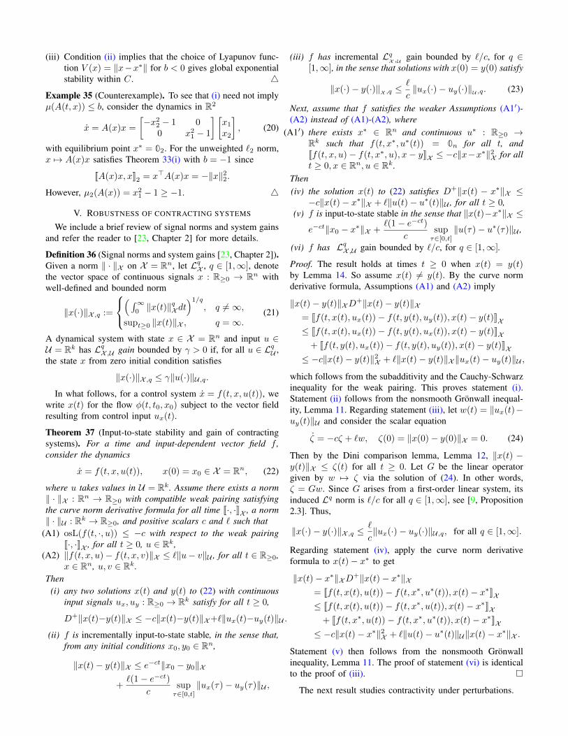
(iii) Condition (ii) implies that the choice of Lyapunov func-tion V (x) = ‖x−x∗‖ for b < 0 gives global exponentialstability within C. 4

Example 35 (Counterexample). To see that (i) need not implyµ(A(t, x)) ≤ b, consider the dynamics in R2

x = A(x)x =

[−x22 − 1 0

0 x21 − 1

] [x1x2

], (20)

with equilibrium point x∗ = 02. For the unweighted `2 norm,x 7→ A(x)x satisfies Theorem 33(i) with b = −1 since

JA(x)x, xK2 = x>A(x)x = −‖x‖22.

However, µ2(A(x)) = x21 − 1 ≥ −1. 4

V. ROBUSTNESS OF CONTRACTING SYSTEMS

We include a brief review of signal norms and system gainsand refer the reader to [23, Chapter 2] for more details.

Definition 36 (Signal norms and system gains [23, Chapter 2]).Given a norm ‖ · ‖X on X = Rn, let LqX , q ∈ [1,∞], denotethe vector space of continuous signals x : R≥0 → Rn withwell-defined and bounded norm

‖x(·)‖X ,q :=

(∫∞

0‖x(t)‖qXdt

)1/q, q 6=∞,

supt≥0 ‖x(t)‖X , q =∞.(21)

A dynamical system with state x ∈ X = Rn and input u ∈U = Rk has LqX ,U gain bounded by γ > 0 if, for all u ∈ LqU ,the state x from zero initial condition satisfies

‖x(·)‖X ,q ≤ γ‖u(·)‖U,q.

In what follows, for a control system x = f(t, x, u(t)), wewrite x(t) for the flow φ(t, t0, x0) subject to the vector fieldresulting from control input ux(t).

Theorem 37 (Input-to-state stability and gain of contractingsystems). For a time and input-dependent vector field f ,consider the dynamics

x = f(t, x, u(t)), x(0) = x0 ∈ X = Rn, (22)

where u takes values in U = Rk. Assume there exists a norm‖ · ‖X : Rn → R≥0 with compatible weak pairing satisfyingthe curve norm derivative formula for all time J·, ·KX , a norm‖ · ‖U : Rk → R≥0, and positive scalars c and ` such that

(A1) osL(f(t, ·, u)) ≤ −c with respect to the weak pairingJ·, ·KX , for all t ≥ 0, u ∈ Rk,

(A2) ‖f(t, x, u)− f(t, x, v)‖X ≤ `‖u− v‖U , for all t ∈ R≥0,x ∈ Rn, u, v ∈ Rk.

Then(i) any two solutions x(t) and y(t) to (22) with continuous

input signals ux, uy : R≥0 → Rk satisfy for all t ≥ 0,

D+‖x(t)−y(t)‖X ≤ −c‖x(t)−y(t)‖X+`‖ux(t)−uy(t)‖U .

(ii) f is incrementally input-to-state stable, in the sense that,from any initial conditions x0, y0 ∈ Rn,

‖x(t)− y(t)‖X ≤ e−ct‖x0 − y0‖X

+`(1− e−ct)

csupτ∈[0,t]

‖ux(τ)− uy(τ)‖U ,

(iii) f has incremental LqX ,U gain bounded by `/c, for q ∈

[1,∞], in the sense that solutions with x(0) = y(0) satisfy

‖x(·)− y(·)‖X ,q ≤`

c‖ux(·)− uy(·)‖U ,q. (23)

Next, assume that f satisfies the weaker Assumptions (A1′)-(A2) instead of (A1)-(A2), where

(A1′) there exists x∗ ∈ Rn and continuous u∗ : R≥0 →Rk such that f(t, x∗, u∗(t)) = 0n for all t, andJf(t, x, u)− f(t, x∗, u), x− yKX ≤ −c‖x−x∗‖2X for allt ≥ 0, x ∈ Rn, u ∈ Rk.

Then(iv) the solution x(t) to (22) satisfies D+‖x(t) − x∗‖X ≤−c‖x(t)− x∗‖X + `‖u(t)− u∗(t)‖U , for all t ≥ 0,

(v) f is input-to-state stable in the sense that ‖x(t)−x∗‖X ≤

e−ct‖x0 − x∗‖X +`(1− e−ct)

csupτ∈[0,t]

‖u(τ)− u∗(τ)‖U ,

(vi) f has LqX ,U gain bounded by `/c, for q ∈ [1,∞].

Proof. The result holds at times t ≥ 0 when x(t) = y(t)by Lemma 14. So assume x(t) 6= y(t). By the curve normderivative formula, Assumptions (A1) and (A2) imply

‖x(t)− y(t)‖XD+‖x(t)− y(t)‖X= Jf(t, x(t), ux(t))− f(t, y(t), uy(t)), x(t)− y(t)KX≤ Jf(t, x(t), ux(t))− f(t, y(t), ux(t)), x(t)− y(t)KX

+ Jf(t, y(t), ux(t))− f(t, y(t), uy(t)), x(t)− y(t)KX≤ −c‖x(t)− y(t)‖2X + `‖x(t)− y(t)‖X ‖ux(t)− uy(t)‖U ,

which follows from the subadditivity and the Cauchy-Schwarzinequality for the weak pairing. This proves statement (i).Statement (ii) follows from the nonsmooth Gronwall inequal-ity, Lemma 11. Regarding statement (iii), let w(t) = ‖ux(t)−uy(t)‖U and consider the scalar equation

ζ = −cζ + `w, ζ(0) = ‖x(0)− y(0)‖X = 0. (24)

Then by the Dini comparison lemma, Lemma 12, ‖x(t) −y(t)‖X ≤ ζ(t) for all t ≥ 0. Let G be the linear operatorgiven by w 7→ ζ via the solution of (24). In other words,ζ = Gw. Since G arises from a first-order linear system, itsinduced Lq norm is `/c for all q ∈ [1,∞], see [9, Proposition2.3]. Thus,

‖x(·)− y(·)‖X ,q ≤`

c‖ux(·)− uy(·)‖U,q, for all q ∈ [1,∞].

Regarding statement (iv), apply the curve norm derivativeformula to x(t)− x∗ to get

‖x(t)− x∗‖XD+‖x(t)− x∗‖X= Jf(t, x(t), u(t))− f(t, x∗, u∗(t)), x(t)− x∗KX≤ Jf(t, x(t), u(t))− f(t, x∗, u(t)), x(t)− x∗KX

+ Jf(t, x∗, u(t))− f(t, x∗, u∗(t)), x(t)− x∗KX≤ −c‖x(t)− x∗‖2X + `‖u(t)− u∗(t)‖U‖x(t)− x∗‖X .

Statement (v) then follows from the nonsmooth Gronwallinequality, Lemma 11. The proof of statement (vi) is identicalto the proof of (iii).

The next result studies contractivity under perturbations.

Theorem 38 (Contraction under perturbations). Consider thedynamics x = f(t, x) + g(t, x). If osL(f(t, ·)) ≤ −c < 0 andosL(g(t, ·)) ≤ d ∈ R with respect to the same weak pairingJ·, ·K for all t ≥ 0, then

(i) (contractivity under perturbations) if d < c, then f + g isstrongly contracting with rate c− d,

(ii) (equilibrium point under perturbations) if additionally fand g are time-invariant, then the unique equilibriumpoint x∗ of f and x∗∗ of f + g satisfy

‖x∗ − x∗∗‖ ≤ ‖g(x∗)‖c− d

. (25)

Proof. Statement (i) is an immediate consequence of Proposi-tion 27(iv). Finally, we consider the two initial value problemsx = f(x) + g(x) and y = f(y) + g(y)− g(x∗) with arbitraryinitial conditions. Note f(x∗) + g(x∗) − g(x∗) = 0, thatis, x∗ is the unique equilibrium of the contracting systemf(y)+g(y)−g(x∗). Taking the limit as t→∞, Theorem 37(ii)implies statement (ii).

VI. NETWORKS OF CONTRACTING SYSTEMS

We consider the interconnection of n dynamical systems

xi = fi(t, xi, x−i), for i ∈ 1, . . . , n, (26)

where xi ∈ RNi , N =∑ni=1Ni, x−i ∈ RN−Ni , and fi :

R≥0 × RNi × RN−Ni → RNi is continuous. Let ‖ · ‖i andJ·, ·Ki denote a norm and a weak pairing on RNi . Assume

(C1) at fixed x−i and t, each map xi 7→ fi(t, xi, x−i) satisfiesosL(f(t, ·, x−i)) ≤ −ci < 0 with respect to J·, ·Ki.

(C2) at fixed xi and t, each map x−i 7→ fi(t, xi, x−i) satisfiesa Lipschitz condition where, for all j ∈ 1, . . . , n \ i,there exists γij ∈ R≥0, such that for all xj , yj ∈ RNj ,

‖fi(t, xi, x−i)− fi(t, xi, y−i)‖i ≤n∑

j=1,j 6=i

γij‖xj − yj‖j .

Lemma 39 (Efficiency of diagonally weighted norm [47,Lemma 3]). Let M ∈ Rn×n be Metzler and let α(M) denoteits spectral abscissa. Then, for each ε > 0, there existsξ ∈ Rn>0 satisfying the LMI

diag(ξ)M +M> diag(ξ) 2(α(M) + ε) diag(ξ). (27)

Moreover, if M is irreducible, the result holds with ε = 0.

Definition 40 (Diagonally weighted aggregation norm). Forξ ∈ Rn>0, define the ξ-weighted norm and corresponding weakpairing on RN by

‖(x1, . . . , xn)‖2ξ =∑n

i=1ξi‖xi‖2i , (28)

J(x1, . . . , xn), (y1, . . . , yn)Kξ =∑n

i=1ξi Jxi, yiKi . (29)

It is easy to see that (28) defines a norm. We prove inAppendix D that (29) is a weak pairing that is compatiblewith (28).

Theorem 41 (Contractivity of interconnected system). Con-sider the interconnection of continuous systems (26) satisfyingAssumptions (C1) and (C2) and define the gain matrix

Γ :=

−c1 . . . γ1n...

...γn1 . . . −cn

.If Γ is Hurwitz, then

(i) for every ε ∈ ]0, |α(Γ)|[, there exists ξ ∈ Rn>0 suchthat the interconnected system is strongly contracting withrespect to ‖ · ‖ξ in (28) with rate |α(Γ) + ε|, and

(ii) if Γ is irreducible, the result (i) holds with ε = 0.

Proof. For i ∈ 1, . . . , n, Assumptions (C1) and (C2) imply

Jfi(t, xi, x−i)− fi(t, yi, y−i), xi − yiKi≤ Jfi(t, xi, x−i)− fi(t, yi, x−i), xi − yiKi

+ Jfi(t, yi, x−i)− fi(t, yi, y−i), xi − yiKi≤ −ci‖xi − yi‖2i +

∑n

j=1,j 6=iγij‖xj − yj‖j‖xi − yi‖i,

where we used the subadditivity and Cauchy-Schwarz inequal-ity for the weak pairing. By Lemma 39, for ε ∈ ]0, |α(Γ)|[,select ξ ∈ Rn>0 satisfying (27). Next, we check the one-sidedLipschitz condition for the interconnected system on RN withrespect to norm (28) and weak pairing (29):∑n

i=1ξi Jfi(t, xi, x−i)− fi(t, yi, y−i), xi − yiKi

≤ −∑n

i=1ξici‖xi − yi‖2i

+∑n

i,j=1,j 6=iξiγij‖xj − yj‖j‖xi − yi‖i

=

‖x1 − y1‖1...‖xn − yn‖n

>

diag(ξ)Γ

‖x1 − y1‖1...‖xn − yn‖n

=

‖x1 − y1‖1...‖xn − yn‖n

>

diag(ξ)Γ + Γ> diag(ξ)

2

‖x1 − y1‖1...‖xn − yn‖n

,so that the interconnected system is strongly contracting if thegain matrix Γ is diagonally stable. Moreover, using Lemma 39∑n

i=1ξi Jfi(t, xi, x−i)− fi(t, yi, y−i), xi − yiKi

≤ (α(Γ) + ε)

‖x1 − y1‖1...‖xn − yn‖n

>

diag(ξ)

‖x1 − y1‖1...‖xn − yn‖n

= (α(Γ) + ε)

∑n

i=1ξi‖xi − yi‖2i

= (α(Γ) + ε)‖(x1 − y1, . . . , xn − yn)‖2ξ .

Then by Theorem 31, we have strong contraction with rate|α(Γ) + ε| and incremental exponential stability. Finally, if Γis irreducible, we can take ε = 0 by Lemma 39.

An example interconnected system satisfying the Assump-tions (C1) and (C2) is of the form fi(t, xi, x−i) = gi(t, xi) +

∑nj=1,j 6=iHijxj , where each vector field gi(t, xi) has one-

sided Lipschitz constant −ci and where Assumption (C2) issatisfied with γij equal to the induced gain of Hij .

Remark 42 (Input-to-state stability and gain of interconnectedcontracting systems). Consider interconnected subsystems ofthe form xi = f(t, xi, x−i, ui) with an input ui ∈ Rki .Assume each fi satisfies Assumptions (C1) and (C2) at fixedinput and, for fixed xi, x−i, t and all ui, vi ∈ Rki ,

‖f(t, xi, x−i, ui)− f(t, xi, x−i, vi)‖i ≤ `i‖ui − vi‖Ui ,

for some norm ‖·‖Ui on Rki . Then, with c = |α(Γ)+ε|, The-orem 37 shows that the interconnected system is incrementallyinput-to-state stable with

‖x(t)− y(t)‖ξ ≤ e−ct‖x0 − y0‖ξ

+1− e−ct

c

∑n

i=1`iξi sup

τ∈[0,t]‖ux,i(τ)− uy,i(τ)‖Ui ,

and has finite incremental LqX ,U gain, for any q ∈ [1,∞]. 4

VII. CONCLUSIONS

This paper presents weak pairings as a novel tool to studycontraction theory with respect to arbitrary norms. Through thelanguage of weak pairings, we prove contraction equivalencesfor continuously differentiable vector fields, continuous vectorfields, and for equilibrium contraction. For `p norms with p ∈[1,∞], we present explicit formulas for the matrix measure,the Demidovich condition, and the one-sided Lipschitz condi-tion, leading to novel contraction equivalences for p ∈ 1,∞.We then prove novel robustness results for contracting andequilibrium contracting systems including incremental input-to-state stability properties as well as finite incremental LqX ,Ugain. Finally, we provide a main interconnection theorem forcontracting subsystems, that provides a counterpart to similartheorems for dissipative subsystems.

Possible directions for future research include (i) leveragingour non-Euclidean conditions for control design akin to controlcontraction metrics [44], (ii) studying the generalization tononsmooth Finsler Lyapunov functions and differentially pos-itive systems [27], [28], (iii) exploring the additional structurein monotone systems [13], and finally (iv) studying generaliza-tions of contraction including partial contraction [56], trans-verse contraction [43], and contraction after transients [45].

VIII. ACKNOWLEDGMENTS

The authors wish to thank Zahra Aminzare, BassamBamieh, Ian Manchester, and Anton Proskurnikov for stim-ulating conversations about contraction theory and systemstheory.

APPENDIX ADEIMLING PAIRINGS

Definition 43 (Deimling pairing [19, Chapter 3]). Given anorm ‖ · ‖ on Rn, the Deimling pairing is the map (·, ·)+ :Rn × Rn → R defined by

(x, y)+ := ‖y‖ limh→0+

‖y + hx‖ − ‖y‖h

. (30)

This limit is known to exist for every x, y ∈ Rn.

If a norm is differentiable, then its associated Lumer pairingcoincides with the Deimling pairing. The Deimling pairing isalso referred to as superior semi-inner product and right semi-inner product, [25, Chapter 3], [5, Remark 1].

Lemma 44 (Deimling pairing properties [25, Chapter 3,Proposition 5 and Corollary 5]). Let ‖ · ‖ be a norm on Rn.Then the following properties hold:

(i) (x1+x2, y)+ ≤ (x1, y)++(x2, y)+ for all x1, x2, y ∈ Rnand (·, ·)+ is continuous in its first argument,

(ii) (αx, y)+ = (x, αy)+ = α(x, y)+ and (−x,−y)+ =(x, y)+ for all x, y ∈ Rn, α ≥ 0,

(iii) (x, x)+ = ‖x‖2 for all x ∈ Rn,(iv) |(x, y)+| ≤ ‖x‖‖y‖ for all x, y ∈ Rn.

While a Deimling pairing need not be a Lumer pairing and aLumer pairing need not be a Deimling pairing, both Deimlingpairings and Lumer pairings are weak pairings.

Lemma 45 (Relationship between Deimling pairing andLumer pairings for a norm [25, Chapter 3, Theorem 20]). Let‖ · ‖ be a norm on Rn and let [·, ·] be a compatible Lumerpairing. Then

[x, y] ≤ (x, y)+, for all x, y ∈ Rn. (31)

Moreover, if Sp is the set of all Lumer pairings compatible withthe norm, then (x, y)+ = sup[·,·]∈Sp

[x, y] for all x, y ∈ Rn.

Lemma 46 (Deimling curve norm derivative formula [19,Proposition 13.1]). Let x : ]a, b[→ Rn be differentiable. Then

‖x(t)‖D+‖x(t)‖ = (x(t), x(t))+, for all t ∈ ]a, b[. (32)

Hence, any Deimling pairing satisfies Deimling’s inequality(by definition) and the curve norm derivative formula (withequality holding for all time).

Remark 47 (Logarithmic Lipschitz constant). In [53, Defini-tion 5.2], the least upper bound logarithmic Lipschitz constantof a map f : C → Rn is defined by

M+(f) := supx6=y

(f(x)− f(y), x− y)+‖x− y‖2

. (33)

In other words, M+(f) is a special case of osL(f), where osLmay be with respect to any weak pairing satisfying Deimling’sinequality. Thus, we show that, in contraction theory, we arenot restricted to using Deimling pairings for analysis. 4

Finally, for comparison’s sake, we report from [19, Exam-ple 13.1(b)], the Deimling pairing for the `1 norm:

(x, y)+,1 = ‖y‖1(

sign(y)>x+∑n

i=1|xi|χ0(yi)

). (34)

APPENDIX BPROOF OF LEMMA 24

Before we prove Lemma 24, we first define a class of Lumerpairings called single-index pairings.

Lemma 48 (Single-index pairings). For R ∈ Rn×n invertible,let ‖ · ‖∞,R be the weighted `∞ norm. Let 2[n] be the power

set of 1, . . . , n. A choice function on 1, . . . , n, f : 2[n] \∅ → 1, . . . , n satisfies for all S ∈ 2[n] \ ∅, f(S) ∈ S.Let Fchoice be the set of all choice functions on 1, . . . , n.Then each f ∈ Fchoice defines a Lumer pairing uniquely:

[x, y]∞,R := (Rx)f(I∞(Ry))(Ry)f(I∞(Ry)). (35)

Moreover, each Lumer pairing is compatible with the weighted`∞ norm.

Proof. First, we prove that any choice function defines aLumer pairing. Let f ∈ Fchoice. Regarding property (i), letx1, x2, y ∈ Rn.

[x1 + x2, y]∞,R = R(x1 + x2)f(I∞(Ry))(Ry)f(I∞(Ry))

= [x1, y]∞,R + [x2, y]∞,R.

For property (ii), let α ∈ R. Then

[αx, y]∞,R = (Rαx)f(I∞(Ry))(Ry)f(I∞(Ry)) = α[x, y]∞,R.

[x, αy]∞,R = (Rx)f(I∞(Rαy))(Rαy)f(I∞(Rαy)) = α[x, y]∞,R.

Regarding property (iii):

[x, x]∞,R = (Rx)f(I∞(Rx))(Rx)f(I∞(Rx)) = ‖x‖2∞,R ≥ 0.

This also proves compatibility. Finally, for property (iv):

|[x, y]∞,R| = |(Rx)f(I∞(Ry))(Ry)f(I∞(Ry))|= ‖Ry‖∞|(Rx)f(I∞(Ry))|≤ ‖Ry‖∞‖Rx‖∞ = [x, x]

1/2∞,R[y, y]

1/2∞,R.

Corollary 49 (Relationship between max pairing and sin-gle-index pairings). Let Sindex be the set of all single-indexpairings on Rn compatible with norm ‖ · ‖∞,R. Then we have

Jx, yK∞,R ≥ [x, y]∞,R, for all [·, ·]∞,R ∈ Sindex, x, y ∈ Rn.

Moreover, for all x, y ∈ Rn, there exists [·, ·]∞,R ∈ Sindex suchthat Jx, yK∞,R = [x, y]∞,R.

Proof. Jx, yK∞,R ≥ [x, y]∞,R follows by definition. More-over, if x, y are fixed, let i∗ = argmaxi∈I∞(Ry)(Ry)i(Rx)i.Then any choice function satisfying f(I∞(Ry)) = i∗ definesa single-index pairing with Jx, yK∞,R = [x, y]∞,R.

Proof of Lemma 24. Let x, y ∈ Rn \ 0n. Then by Corol-lary 49, there exists [·, ·]∞,R ∈ Sindex such that Jx, yK∞,R =[x, y]∞,R. However, since [·, ·]∞,R is a Lumer pairing, itsatisfies Deimling’s inequality. Thus,

Jx, yK∞,R = [x, y]∞,R

≤ ‖y‖∞,R limh→0+

‖y + hx‖∞,R − ‖y‖∞,Rh

.

Since x, y were arbitrary, this proves the result.

APPENDIX CPROOF OF PROPOSITION 27

To prove Proposition 27, we will first prove one additionalproperty of weak pairings.

Lemma 50. Let ‖ · ‖ be a norm on Rn with compatible weakpairing J·, ·K satisfying Deimling’s inequality. Then for all x ∈Rn, c ∈ R:

Jcx, xK = c‖x‖2. (36)

Proof. If c ≥ 0, the result is trivial, so without loss ofgenerality, assume c = −1. Lumer’s equality, Theorem 18,with A = −In implies for all x ∈ Rn

supx 6=0n

J−x, xK‖x‖2

= µ(−In) = −1 =⇒ J−x, xK ≤ −‖x‖2.

Regarding the other inequality, observe that

Jx, xK = Jx− x+ x, xK ≤ J−x, xK + 2 Jx, xK=⇒ J−x, xK ≥ − Jx, xK = −‖x‖2.

By weak homogeneity, this proves the result.

Proof of Proposition 27. Properties (i), (iii), and (iv) are con-sequences of Cauchy-Schwarz, weak homogeneity, and sub-additivity of the weak pairing, respectively. Regarding prop-erty (ii), we will show the more general result that for anyx, y ∈ C, c ∈ R, Jx+ cy, yK = Jx, yK + c‖y‖2. The inequality

Jx+ cy, yK ≤ Jx, yK + c‖y‖2,

follows from subadditivity and Lemma 50. Additionally,

Jx, yK = Jx+ cy − cy, yK ≤ Jx+ cy, yK + J−cy, yK= Jx+ cy, yK− c‖y‖2,

where the final equality holds by Lemma 50. Rearranging theinequality implies the result.

APPENDIX DSUM DECOMPOSITION OF WEAK PAIRINGS

Lemma 51 (Weak pairing sum decomposition). For N =∑ni=1Ni, let x = (x1, . . . , xn), y = (y1, . . . , yn) ∈ RN and

xi, yi ∈ RNi . Let ‖·‖i and J·, ·Ki denote a norm and compatibleweak pairing on RNi and let ξ ∈ Rn>0. Then the mappingJ·, ·K : RN × RN → RN defined by

Jx, yK :=∑n

i=1ξi Jxi, yiKi ,

is a weak pairing compatible with the norm ‖x‖2ξ =∑ni=1 ξi‖xi‖2i .

Proof. We verify the properties in Definition 15. Regard-ing property (i), let x1, x2, y ∈ RN . Then Jx1 + x2, yK =∑ni=1 ξi Jx1i + x2i , yiKi ≤

∑ni=1 ξi Jx1i , yiKi+ ξi Jx2i , yiKi =

Jx1, yK+Jx2, yK. Continuity in the first argument follows fromcontinuity of the first argument of each of the J·, ·Ki. Regardingproperty (ii), the result is straightforward because of weakhomogeneity of each of the J·, ·Ki. Regarding property (iii),

Jx, xK =

n∑i=1

ξi Jxi, xiKi =

n∑i=1

ξi‖xi‖2i > 0, for all x 6= 0N .

Regarding property (iv), since n is finite, by induction itsuffices to check n = 2. For convenience, define ai =ξi Jxi, xiKi , bi = ξi Jyi, yiKi. Then

Jx, yK2 =(∑2

i=1ξi Jxi, yiKi

)2≤(∑2

i=1a1/2i b

1/2i

)2= (√a1b1 +

√a2b2)2 = a1b1 + a2b2 + 2

√a1b1a2b2

≤ a1b1 + a2b2 + a1b2 + a2b1 = (a1 + a2)(b1 + b2)

=(∑2

i=1ai

)(∑2

i=1bi

)= Jx, xK Jy, yK ,

where we have used Cauchy-Schwarz for the J·, ·Ki and theinequality 2

√αβ ≤ α + β for α, β ≥ 0. Taking the square

root of each side proves the result.

APPENDIX ESEMI-CONTRACTION EQUIVALENCES

We recall semi-norms and some of their properties and referto [33] for more details.

Definition 52 (Semi-norms). A map |||·||| : Rn → R≥0 is asemi-norm on Rn if

(i) |||cv||| = |c||||v||| for all v ∈ R, c ∈ R;(ii) |||v + w||| ≤ |||v|||+ |||w|||, for all v, w ∈ Rn.

For a semi-norm |||·|||, its kernel is defined by

Ker |||·||| = v ∈ Rn | |||v||| = 0.

Note that Ker |||·||| is a subspace of Rn and that |||·||| is a normon Ker |||·|||⊥. Since Ker |||·|||⊥ ∼= Rm for some m ≤ n, weare able to define weak pairings on Ker |||·|||⊥.

Definition 53 (Induced semi-norm). Let |||·||| be a semi-normon Rn. The induced semi-norm is a map |||·||| : Rn×n → R≥0defined by

|||A||| := sup|||Av|||/|||v||| | v ∈ Ker |||·|||⊥ \ 0n

.

Definition 54 (Matrix semi-measures). Let |||·||| be a semi-norm on Rn and its corresponding induced semi-norm onRn×n. Then the matrix semi-measure associated with |||·||| isdefined by

µ|||·|||(A) := limh→0+

|||In + hA||| − 1

h.

We refer to [33, Proposition 3 and Theorem 5] for propertiesof induced semi-norms and matrix semi-measures.

We specialize to consider semi-norms of the form |||v||| =‖Pv‖ where either P ∈ Rm×n is a rank m matrix for m ≤ nand ‖·‖ is a norm on Rm or P ∈ Rn×n with rank m ≤ n and‖ · ‖ is a norm on Rn. To make this convention clear, we say|||·||| = ‖P · ‖. Then clearly Ker |||·||| = KerP . First, we provea useful lemma resembling Lumer’s equality, Theorem 18.

Lemma 55 (Lumer’s equality for matrix semi-measures). Let|||·||| = ‖P · ‖ be a semi-norm on Rn with compatible weakpairing J·, ·K on Ker |||·|||⊥ satisfying Deimling’s inequality.Then for all A ∈ Rn×n satisfying AKer |||·||| ⊆ Ker |||·|||

µ|||·|||(A) = supx∈Ker |||·|||⊥\0n

JPAx,PxK|||x|||2

(37)

= supx/∈Ker |||·|||

JPAx,PxK|||x|||2

. (38)

Proof. First we show the equivalence of (37) and (38). ClearlyJPAx,PxK|||x|||2

| x ∈ Ker |||·|||⊥ \ 0n

⊆JPAx,PxK

|||x|||2| x /∈ Ker |||·|||

.

Regarding the other containment, let x /∈ Ker |||·|||. Then sinceRn = Ker |||·||| ⊕Ker |||·|||⊥, there exist xKer ∈ Ker |||·|||, x⊥ ∈Ker |||·|||⊥ \ 0n such that x = xKer + x⊥. Then

JPAx,PxK|||x|||2

=JPA(xKer + x⊥),P(xKer + x⊥)K

‖P(xKer + x⊥)‖2

=JPAx⊥,Px⊥K|||x⊥|||2

.

Where the second equality holds because Ker |||·||| = KerPand AKer |||·||| ⊆ Ker |||·|||. Therefore,JPAx,PxK

|||x|||2| x ∈ Ker |||·|||⊥ \ 0n

⊇JPAx,PxK

|||x|||2| x /∈ Ker |||·|||

.

This proves that the two sets are equal and therefore theirsupremums are equal. Next, we show that µ|||·|||(A) ≥supx∈Ker |||·|||⊥\0n

JPAx,PxK|||x|||2 . By Deimling’s inequality, for

every x ∈ Ker |||·|||⊥ \ 0n,

JPAx,PxK ≤ ‖Px‖ limh→0+

‖Px+ hPAx‖ − ‖Px‖h

= |||x||| limh→0+

|||(In + hA)x||| − |||x|||h

≤ |||x|||2 limh→0+

|||In + hA||| − 1

h= |||x|||2µ|||·|||(A) ,

where the third line follows since |||Ax||| ≤ |||A||||||x||| forevery x ∈ Ker |||·|||⊥. This proves this inequality. Regard-ing the other direction, for v /∈ Ker |||·|||, define Ω(v) =JPAv,PvK /|||v|||2.Then for every v /∈ Ker |||·|||,

|||(In − hA)v||| ≥ 1

|||v|||JP(In − hA)v,PvK

≥ (1− hΩ(v))|||v||| ≥ (1− h supv/∈Ker |||·|||

Ω(v))|||v|||,

where the first inequality holds because of Cauchy-Schwarz,the second because of subadditivity of the weak pairing, andthe final one because −h < 0. Then for small enough h > 0,In−hA is invertible and given by (In−hA)−1 = In+hA+h2A2(In − hA)−1, which implies

|||(In + hA)v||| ≤∣∣∣∣∣∣(In − hA)−1v

∣∣∣∣∣∣+h2∣∣∣∣∣∣A2(In − hA)−1v∣∣∣∣∣∣,

where the implication holds for all v ∈ Rn because ofthe triangle inequality for semi-norms. Moreover, let x ∈Ker |||·|||⊥\0n and define v = (In−hA)−1x. To see that v /∈Ker |||·|||, suppose for contradiction’s sake that v ∈ Ker |||·|||.Then since (In − hA)v = x, we have v − hAv = x. ButhAv ∈ Ker |||·||| since, by assumption, AKer |||·||| ⊆ Ker |||·|||.

And since Ker |||·||| is a subspace, v − hAv = x ∈ Ker |||·|||, acontraction. Therefore v /∈ Ker |||·|||. Then for h > 0, we have∣∣∣∣∣∣(In − hA)−1x

∣∣∣∣∣∣|||x|||

=|||v|||

|||(In − hA)v|||

≤ 1

1− h supv/∈Ker |||·||| Ω(v). (39)

Then

µ|||·|||(A) = limh→0+

supx∈Ker |||·|||⊥\0n

|||(In + hA)x|||/|||x||| − 1

h

≤ limh→0+

supx∈Ker |||·|||⊥\0n

(∣∣∣∣∣∣(In − hA)−1x∣∣∣∣∣∣/|||x||| − 1

h

+h2∣∣∣∣∣∣A2(In − hA)−1x

∣∣∣∣∣∣h|||x|||

)≤ limh→0+

supx∈Ker |||·|||⊥\0n

∣∣∣∣∣∣(In − hA)−1x∣∣∣∣∣∣/|||x||| − 1

h

≤ limh→0+

1

h

( 1

1− h supv/∈Ker |||·||| Ω(v)− 1)

= supx/∈Ker |||·|||

JPAx,PxK|||x|||2

,

where the second line holds because of the triangle inequality,the third line holds because of the subadditivity of the supre-mum, and the fourth line holds because the inequality in (39)holds for all x ∈ Ker |||·|||⊥ \0n. This proves the result.

Lemma 56 (Coppel’s differential inequality for semi-norms).Let |||·||| = ‖P·‖ be a seminorm on Rn. Consider the dynamicalsystem x = A(t, x)x where (t, x) 7→ A(t, x) ∈ Rn×n iscontinuous in (t, x). Moreover, assume for all x ∈ Rn, t ∈R≥0, Ker |||·||| is invariant under A(t, x) in the sense thatA(t, x) Ker |||·||| ⊆ Ker |||·|||. Then

D+|||x(t)||| ≤ µ|||·|||(A(t, x(t))) |||x(t)|||.

Proof. First assume that |||x(t)||| = 0 for some t ≥ 0. Thenx(t) ∈ Ker |||·|||, and by assumption A(t, x)x(t) ∈ Ker |||·|||.Then by computation:

D+|||x(t)||| = lim suph→0+

|||x(t+ h)||| − |||x(t)|||h

= lim suph→0+

|||x(t) + hA(t, x(t))x(t)|||h

≤ lim suph→0+

|h||||A(t, x)x(t)|||h

= |||A(t, x)x(t)||| = 0.

So the result holds in this case. So assume |||x(t)||| 6= 0, i.e.,x(t) /∈ Ker |||·|||. Then apply the curve norm derivative formulafor Deimling pairings, Lemma 46 to |||x(t)|||:

|||x(t)|||D+|||x(t)||| = (PA(t, x(t))x(t),Px(t))+

=⇒ D+|||x(t)||| = (PA(t, x(t))x(t),Px(t))+

|||x(t)|||2|||x(t)|||

≤ µ|||·|||(A(t, x(t))) |||x(t)|||,

where the inequality holds by Lemma 55 since (·, ·)+ is aweak pairing that trivially satisfies Deimling’s inequality.

We now prove semi-contraction theorems analogous tothe contraction theorem for continuously differentiable vectorfields, Theorem 29, and the equilibrium contraction theorem,Theorem 33.

Theorem 57 (Semi-contraction theorem for continuouslydifferentiable vector fields). Consider the dynamical systemx = f(t, x), which is continuously differentiable in x withJacobian Df . Let |||·||| = ‖P · ‖ be a semi-norm on Rn. LetJ·, ·K be a weak pairing on Ker |||·|||⊥ satisfying Deimling’sinequality. Moreover, assume Df(t, x) Ker |||·||| ⊆ Ker |||·||| forall t ≥ 0, x ∈ Rn. Then, for b ∈ R, the following statementsare equivalent:

(i) µ|||·|||(Df(t, x)) ≤ b, for all x ∈ Rn, t ≥ 0,(ii) JPDf(t, x)v,PvK ≤ b|||v|||2, for all v ∈ Rn, x ∈ Rn, t ≥

0,(iii) JP(f(t, x)− f(t, y)),P(x− y)K ≤ b|||x− y|||2, for all

x, y ∈ Rn, t ≥ 0,

(iv) D+|||φ(t, t0, x0) − φ(t, t0, y0)||| ≤ b|||φ(t, t0, x0) −φ(t, t0, y0)|||, for all x0, y0 ∈ Rn, 0 ≤ t0 ≤ t for whichsolutions exist,

(v) |||φ(t, t0, x0) − φ(t, t0, y0)||| ≤ eb(t−s)|||φ(s, t0, x0) −φ(s, t0, y0)|||, for all x0, y0 ∈ Rn, 0 ≤ t0 ≤ s ≤ t forwhich solutions exist.

Proof. Regarding (i) ⇐⇒ (ii), the proof follows by Lumer’sequality for matrix semi-measures, Lemma 55.

Regarding (ii) =⇒ (iii), suppose JPDf(t, z)v,PvK ≤b|||v|||2, for all v ∈ Rn, z ∈ Rn, t ≥ 0. Then let x, y ∈ Rnand v = x− y. By the mean-value theorem for vector-valuedfunctions, we have

f(t, x)− f(t, y) =

(∫ 1

0

Df(t, y + sv)ds

)(x− y).

Hence,

JP(f(t, x)− f(t, y)),P(x− y)K

=

sP(∫ 1

0

Df(t, y + sv)ds

)(x− y),P(x− y)

=

s(∫ 1

0

PDf(t, y + sv)ds

)(x− y),P(x− y)

≤∫ 1

0

JPDf(t, y + sv)(x− y),P(x− y)K ds

≤∫ 1

0

b|||x− y|||2ds = b|||x− y|||2,

where the third line follows from the sublinearity and conti-nuity in the first argument of the weak pairing.

Regarding (iii) =⇒ (ii), assumeJP(f(t, x)− f(t, y)),P(x− y)K ≤ b|||x− y|||2, for allx, y ∈ Rn, t ≥ 0. If x = y, the result is trivial, soassume x 6= y. Fix y and set x = y + hv for an arbitraryv ∈ Rn, h ∈ R>0. Then substituting

JP(f(t, y + hv)− f(t, y)),PhvK ≤ b|||hv|||2

=⇒ h JP(f(t, y + hv)− f(t, y)),PvK ≤ bh2|||v|||2,

by the weak homogeneity of the weak pairing. Dividing byh2 and taking the limit as h goes to zero yields

limh→0+

sP f(t, y + hv)− f(t, y)

h,Pv

≤ b|||v|||2

=⇒ JPDf(t, y)v,PvK ≤ b|||v|||2,

which follows from the continuity of the weak pairing in itsfirst argument. Since y, v, and t were arbitrary, this completesthis implication.

Regarding (i) =⇒ (iv), let x0, y0 ∈ Rn, t0 ≥ 0 and letx(t) = φ(t, t0, x0), y(t) = φ(t, t0, y0). Then by the mean-value theorem for vector-valued functions, for v(t) = x(t) −y(t),

v =(∫ 1

0

Df(t, y + sv)ds)v.

Then since Df(t, x) Ker |||·||| ⊆ Ker |||·||| for all t ≥ 0, x ∈ Rn,by Coppel’s differential inequality for semi-norms, Lemma 56,

D+|||v(t)||| ≤ µ|||·|||(∫ 1

0

Df(t, y(t) + sv(t))ds

)|||v(t)|||

≤∫ 1

0

µ|||·|||(Df(t, y(t) + sv(t))) ds |||v(t)|||

≤∫ 1

0

bds |||v(t)||| = b|||v(t)|||,

which holds by the subadditivity of matrix semi-measures.Regarding (iv) =⇒ (v), the result follows by the nons-

mooth Gronwall inequality.Regarding (v) =⇒ (iii), let x0, y0 ∈ C, t0 ≥ 0 be arbitrary.

Then for h ≥ 0,

|||φ(t0 + h, t0, x0)− φ(t0 + h, t0, y0)|||= |||x0 − y0 + h(f(t0, x0)− f(t0, y0))|||+O(h2)

≤ ebh|||x0 − y0|||.

Subtracting |||x0 − y0||| on both sides, dividing by h > 0 andtaking the limit as h→ 0+, we get

limh→0+

|||x0 − y0 + h(f(t0, x0)− f(t0, y0))||| − |||x0 − y0|||h

≤ limh→0+

ebh − 1

h|||x0 − y0|||.

Evaluating the right hand side limit gives

limh→0+

|||x0 − y0 + h(f(t0, x0)− f(t0, y0))||| − |||x0 − y0|||h

≤ b|||x0 − y0|||.

But by the assumption of Deimling’s inequality, multiplyingboth sides by |||x0 − y0||| gives

JP(f(t0, x0)− f(t0, y0)),P(x0 − y0)K ≤ b|||x0 − y0|||2.

Since t0, x0 and y0 were arbitrary, the result holds.

Remark 58. In [33, Theorem 13], (i) =⇒ (v) is proved.Theorem 57 generalizes this result and provides necessary andsufficient conditions for semi-contraction analogous to thosein Theorem 29 including a one-sided Lipschitz condition onthe vector field via the semi-norm.

Theorem 59 (Subspace contraction equivalences). Considerthe dynamical system x = f(t, x), which is continuous in(t, x). Let |||·||| = ‖P · ‖ be a semi-norm on Rn. Let J·, ·K bea weak pairing on Ker |||·|||⊥ satisfying Deimling’s inequalityand the curve norm derivative formula. Moreover, assume thatthere exists x∗ ∈ Ker |||·|||⊥ such that f(t, x∗ + Ker |||·|||) ⊆Ker |||·||| for all t ≥ 0. Then, for b ∈ R, the followingstatements are equivalent:

(i) JPf(t, x),P(x− x∗)K ≤ b|||x− x∗|||2, for all x ∈Rn, t ≥ 0,

(ii) D+|||φ(t, t0, x0)− x∗||| ≤ b|||φ(t, t0, x0)− x∗|||, for allx0, 0 ≤ t0 ≤ t for which solutions exist,

(iii) |||φ(t, t0, x0)− x∗||| ≤ eb(t−s)|||φ(s, t0, x0)− x∗|||, for allx0 ∈ Rn, 0 ≤ t0 ≤ s ≤ t for which solutions exist.

Moreover, suppose that f(t, x) is continuously differentiablein x and that µ|||·|||(Df(t, x)) ≤ b for all (t, x). Then state-ments (i), (ii), and (iii) hold.

Proof. Regarding (i) =⇒ (iii), let x0 ∈ Rn, t0 ≥ 0 and letx(t) = φ(t, t0, x0), y(t) = φ(t, t0, y0). Then we have twocases. If there exists t ≥ t0 such that |||x(t)− x∗||| = 0,then note that x(t) − x∗ ∈ Ker |||·|||, which implies x(t) ∈x∗ + Ker |||·|||, which further implies |||f(t, x(t))||| = 0 byassumption. Then we compute

D+|||x(t)− x∗||| = lim suph→0+

|||x(t+ h)− x∗||| − |||x(t)− x∗|||h

= lim suph→0+

|||x(t)− x∗ + hf(t, x(t))|||h

≤ lim suph→0+

|h||||f(t, x(t))|||h

= |||f(t, x(t))||| = 0.

Then for all t ≥ t0 for which |||x(t)− x∗||| 6= 0, apply thecurve norm derivative to get

|||x(t)− x∗|||D+|||x(t)− x∗||| = JPf(t, x(t)),P(x(t)− x∗)K=⇒ D+|||x(t)− x∗||| ≤ b|||x(t)− x∗|||,

for almost every t ≥ 0. Then applying the nonsmoothGronwall inequality, Lemma 11 gives the desired result.

Regarding (ii) =⇒ (iii), the result follows by the nons-mooth Gronwall inequality.

Regarding (iii) =⇒ (i), let x0 ∈ C, t0 ≥ 0 be arbitrary.Then for h ≥ 0,

|||φ(t0 + h, t0, x0)− x∗|||= |||x0 − x∗ + hf(t0, x0)|||+O(h2)

≤ ebh|||x0 − x∗|||.

Subtracting |||x0 − x∗||| on both sides, dividing by h > 0 andtaking the limit as h→ 0+, we get

limh→0+

|||x0 − x∗ + hf(t0, x0)||| − |||x0 − x∗|||h

≤ limh→0+

ebh − 1

h|||x0 − x∗|||.

Evaluating the right hand side limit gives

limh→0+

|||x0 − x∗ + hf(t0, x0)||| − |||x0 − x∗|||h

≤ b|||x0 − x∗|||.

But by the assumption of Deimling’s inequality, multiplyingboth sides by |||x0 − x∗||| gives

JPf(t0, x0),P(x0 − x∗)K ≤ b|||x0 − x∗|||2.

Since t0 and x0 were arbitrary, the result holds.Regarding (iii) =⇒ (ii), following the proof of (iii) =⇒

(i), the inequality

(Pf(t, x),P(x− x∗))+ ≤ b|||x− x∗|||2, (40)

holds for all x ∈ Rn, t ≥ 0, where the Deimling pairing isdefined on Ker |||·|||⊥. Then applying the curve norm derivativefor the Deimling pairing, Lemma 46 on |||φ(t, t0, x0)− x∗|||proves the result.

Further, suppose f(t, x) is continuously differentiable andµ|||·|||(Df(t, x)) ≤ b for all x ∈ Rn, t ≥ 0. Then [33,Theorem 13(ii)] implies that (iii) holds.

Remark 60. Subspace contraction is a form of equilibriumcontraction for semi-contracting systems. In [33, Theorem 13],µ|||·|||(Df(t, x)) ≤ b =⇒ (iii) is proved. However, Theo-rem 59 gives necessary and sufficient conditions analogousto those in Theorem 33 and demonstrates that weak pairingsare a suitable tool for checking semi-contraction and subspacecontraction.

REFERENCES

[1] M. A. Al-Radhawi and D. Angeli. New approach to the stabilityof chemical reaction networks: Piecewise linear in rates Lyapunovfunctions. IEEE Transactions on Automatic Control, 61(1):76–89, 2016.doi:10.1109/TAC.2015.2427691.

[2] Z. Aminzare. On Synchronous Behavior in Complex Nonlinear Dynam-ical Systems. PhD thesis, Rutgers, 2015.

[3] Z. Aminzare, Y. Shafi, M. Arcak, and E. D. Sontag. Guaranteeingspatial uniformity in reaction-diffusion systems using weighted L2 normcontractions. In A Systems Theoretic Approach to Systems and SyntheticBiology I: Models and System Characterizations, chapter 3, pages 73–101. Springer, 2014. doi:10.1007/978-94-017-9041-3_3.

[4] Z. Aminzare and E. D. Sontag. Logarithmic Lipschitz norms anddiffusion-induced instability. Nonlinear Analysis: Theory, Methods& Applications, 83:31–49, 2013. doi:10.1016/j.na.2013.01.001.

[5] Z. Aminzare and E. D. Sontag. Contraction methods for nonlinearsystems: A brief introduction and some open problems. In IEEEConf. on Decision and Control, pages 3835–3847, December 2014.doi:10.1109/CDC.2014.7039986.

[6] Z. Aminzare and E. D. Sontag. Synchronization of diffusively-connectednonlinear systems: Results based on contractions with respect to generalnorms. IEEE Transactions on Network Science and Engineering,1(2):91–106, 2014. doi:10.1109/TNSE.2015.2395075.

[7] D. Angeli. A Lyapunov approach to incremental stability properties.IEEE Transactions on Automatic Control, 47(3):410–421, 2002. doi:10.1109/9.989067.

[8] M. Arcak, C. Meissen, and A. Packard. Networks of DissipativeSystems: Compositional Certification of Stability, Performance, andSafety. Springer, 2016, ISBN 978-3-319-29928-0. doi:10.1007/978-3-319-29928-0.

[9] B. Bamieh and M. Dahleh. On robust stability with structured time-invariant perturbations. Systems & Control Letters, 21(2):103–108, 1993.doi:10.1016/0167-6911(93)90112-J.

[10] T. Caraballo and P. E. Kloeden. The persistence of synchronization underenvironmental noise. Proceedings of the Royal Society A: Mathematical,Physical and Engineering Sciences, 461(2059):2257–2267, 2005. doi:10.1098/rspa.2005.1484.

[11] L. Chua and D. Green. A qualitative analysis of the behavior ofdynamic nonlinear networks: Stability of autonomous networks. IEEETransactions on Circuits and Systems, 23(6):355–379, 1976. doi:10.1109/TCS.1976.1084228.

[12] G. Como, E. Lovisari, and K. Savla. Throughput optimality and over-load behavior of dynamical flow networks under monotone distributedrouting. IEEE Transactions on Control of Network Systems, 2(1):57–67,2015. doi:10.1109/TCNS.2014.2367361.

[13] S. Coogan. A contractive approach to separable Lyapunov functions formonotone systems. Automatica, 106:349–357, 2019. doi:10.1016/j.automatica.2019.05.001.

[14] S. Coogan and M. Arcak. A compartmental model for traffic networksand its dynamical behavior. IEEE Transactions on Automatic Control,60(10):2698–2703, 2015. doi:10.1109/TAC.2015.2411916.

[15] W. A. Coppel. Stability and Asymptotic Behavior of DifferentialEquations. Heath, 1965, ISBN 0669190187.

[16] G. Dahlquist. Stability and error bounds in the numerical integration ofordinary differential equations. PhD thesis, (Reprinted in Trans. RoyalInst. of Technology, No. 130, Stockholm, Sweden, 1959), 1958.

[17] Luis D’Alto and Martin Corless. Incremental quadratic stability. Nu-merical Algebra, Control and Optimization, 3:175–201, 2013. doi:10.3934/naco.2013.3.175.

[18] J. M. Danskin. The theory of max-min, with applications. SIAMJournal on Applied Mathematics, 14(4):641–664, 1966. doi:10.1137/0114053.

[19] K. Deimling. Nonlinear Functional Analysis. Springer, 1985, ISBN3-540-13928-1.

[20] P. DeLellis, M. Di Bernardo, and G. Russo. On QUAD, Lipschitz,and contracting vector fields for consensus and synchronization ofnetworks. IEEE Transactions on Circuits and Systems I: Regular Papers,58(3):576–583, 2011. doi:10.1109/TCSI.2010.2072270.

[21] B. P. Demidovic. Dissipativity of a nonlinear system of differentialequations. Uspekhi Matematicheskikh Nauk, 16(3(99)):216, 1961.

[22] C. A. Desoer and H. Haneda. The measure of a matrix as a tool toanalyze computer algorithms for circuit analysis. IEEE Transactions onCircuit Theory, 19(5):480–486, 1972. doi:10.1109/TCT.1972.1083507.

[23] C. A. Desoer and M. Vidyasagar. Feedback Systems: Input-OutputProperties. Academic Press, 1975, ISBN 978-0-12-212050-3. doi:10.1137/1.9780898719055.

[24] M. Di Bernardo, D. Liuzza, and G. Russo. Contraction analysis fora class of nondifferentiable systems with applications to stability andnetwork synchronization. SIAM Journal on Control and Optimization,52(5):3203–3227, 2014. doi:10.1137/120883001.

[25] S. S. Dragomir. Semi-Inner Products and Applications. Nova SciencePublishers, 2004.

[26] A. F. Filippov. Differential Equations with Discontinuous RighthandSides. Kluwer, 1988, ISBN 902772699X.

[27] F. Forni and R. Sepulchre. A differential Lyapunov framework for con-traction analysis. IEEE Transactions on Automatic Control, 59(3):614–628, 2014. doi:10.1109/TAC.2013.2285771.

[28] F. Forni and R. Sepulchre. Differentially positive systems. IEEETransactions on Automatic Control, 61(2):346–359, 2016. doi:10.1109/TAC.2015.2437523.

[29] J. R. Giles. Classes of semi-inner-product spaces. Transactions ofthe American Mathematical Society, 129(3):436–446, 1967. doi:10.2307/1994599.

[30] E. Hairer, S. P. Nørsett, and G. Wanner. Solving Ordinary DifferentialEquations I. Nonstiff Problems. Springer, 1993. doi:10.1007/978-3-540-78862-1.

[31] A. Hamadeh, E. Sontag, and D. Del Vecchio. A contraction approach toinput tracking via high gain feedback. In IEEE Conf. on Decision andControl, pages 7689–7694, December 2015. doi:10.1109/CDC.2015.7403435.

[32] J. A. Jacquez and C. P. Simon. Qualitative theory of compartmentalsystems. SIAM Review, 35(1):43–79, 1993. doi:10.1137/1035003.

[33] S. Jafarpour, P. Cisneros-Velarde, and F. Bullo. Weak and semi-contraction for network systems and diffusively-coupled oscillators.IEEE Transactions on Automatic Control, 2021. To appear. doi:10.1109/TAC.2021.3073096.

[34] H. K. Khalil. Nonlinear Systems. Prentice Hall, 3 edition, 2002, ISBN0130673897.

[35] N. N. Krasovskiı. Stability of Motion. Applications of Lyapunov’s SecondMethod to Differential Systems and Equations with Delay. StanfordUniversity Press, 1963. Translation of the 1959 edition in Russian byJ. L. Brenner.

[36] D. C. Lewis. Metric properties of differential equations. American Jour-nal of Mathematics, 71(2):294–312, 1949. doi:10.2307/2372245.

[37] W. Lohmiller and J.-J. E. Slotine. On contraction analysis for non-linear systems. Automatica, 34(6):683–696, 1998. doi:10.1016/S0005-1098(98)00019-3.

[38] T. Lorenz. Mutational Analysis: A Joint Framework For CauchyProblems In And Beyond Vector Spaces. Springer, 2010, ISBN 978-3-642-12471-6.

[39] S. M. Lozinskii. Error estimate for numerical integration of ordinarydifferential equations. I. Izvestiya Vysshikh Uchebnykh Zavedenii.Matematika, 5:52–90, 1958.

[40] W. Lu and T. Chen. New approach to synchronization analysis of linearlycoupled ordinary differential systems. Physica D: Nonlinear Phenom-ena, 213(2):214–230, 2006. doi:10.1016/j.physd.2005.11.009.

[41] G. Lumer. Semi-inner-product spaces. Transactions of the Amer-ican Mathematical Society, 100:29–43, 1961. doi:10.1090/S0002-9947-1961-0133024-2.

[42] H. Maeda, S. Kodama, and Y. Ohta. Asymptotic behavior of nonlinearcompartmental systems: Nonoscillation and stability. IEEE Transactionson Circuits and Systems, 25(6):372–378, 1978. doi:10.1109/TCS.1978.1084490.

[43] I. R. Manchester and J.-J. E. Slotine. Transverse contraction criteria forexistence, stability, and robustness of a limit cycle. Systems & ControlLetters, 63:32–38, 2014. doi:10.1016/j.sysconle.2013.10.005.

[44] I. R. Manchester and J.-J. E. Slotine. Control contraction metrics:Convex and intrinsic criteria for nonlinear feedback design. IEEETransactions on Automatic Control, 62(6):3046–3053, 2017. doi:10.1109/TAC.2017.2668380.

[45] M. Margaliot, E. D. Sontag, and T. Tuller. Contraction after smalltransients. Automatica, 67:178–184, 2016. doi:10.1016/j.automatica.2016.01.018.

[46] J. Monteil, G. Russo, and R. Shorten. On L∞ string stabilityof nonlinear bidirectional asymmetric heterogeneous platoon systems.Automatica, 105:198–205, 2019. doi:10.1016/j.automatica.2019.03.025.

[47] O. Pastravanu and M. Voicu. Generalized matrix diagonal stabilityand linear dynamical systems. Linear Algebra and its Applications,419(2):299–310, 2006. doi:10.1016/j.laa.2006.04.021.

[48] A. Pavlov, A. Pogromsky, N. Van de Wouw, and H. Nijmeijer. Con-vergent dynamics, a tribute to Boris Pavlovich Demidovich. Sys-tems & Control Letters, 52(3-4):257–261, 2004. doi:10.1016/j.sysconle.2004.02.003.

[49] H. Qiao, J. Peng, and Z.-B. Xu. Nonlinear measures: A new approachto exponential stability analysis for Hopfield-type neural networks.IEEE Transactions on Neural Networks, 12(2):360–370, 2001. doi:10.1109/72.914530.

[50] G. Russo, M. Di Bernardo, and E. D. Sontag. Global entrainment oftranscriptional systems to periodic inputs. PLOS Computational Biology,6(4):e1000739, 2010. doi:10.1371/journal.pcbi.1000739.

[51] G. Russo, M. Di Bernardo, and E. D. Sontag. A contraction approachto the hierarchical analysis and design of networked systems. IEEETransactions on Automatic Control, 58(5):1328–1331, 2013. doi:10.1109/TAC.2012.2223355.

[52] J. W. Simpson-Porco and F. Bullo. Contraction theory on Riemannianmanifolds. Systems & Control Letters, 65:74–80, 2014. doi:10.1016/j.sysconle.2013.12.016.

[53] G. Soderlind. The logarithmic norm. History and modern theory.BIT Numerical Mathematics, 46(3):631–652, 2006. doi:10.1007/s10543-006-0069-9.

[54] T. Strom. On logarithmic norms. SIAM Journal on Numerical Analysis,12(5):741–753, 1975. doi:10.1137/0712055.

[55] M. Vidyasagar. Nonlinear Systems Analysis. SIAM, 2002, ISBN9780898715262. doi:10.1137/1.9780898719185.

[56] W. Wang and J.-J. E. Slotine. On partial contraction analysis for couplednonlinear oscillators. Biological Cybernetics, 92(1):38–53, 2005. doi:10.1007/s00422-004-0527-x.